Point-based Value Iteration for
Neuro-Symbolic POMDPs

Abstract

Neuro-symbolic artificial intelligence is an emerging area that combines traditional symbolic techniques with neural networks. In this paper, we consider its application to sequential decision making under uncertainty. We introduce neuro-symbolic partially observable Markov decision processes (NS-POMDPs), which model an agent that perceives a continuous-state environment using a neural network and makes decisions symbolically, and study the problem of optimising discounted cumulative rewards. This requires functions over continuous-state beliefs, for which we propose a novel piecewise linear and convex representation (P-PWLC) in terms of polyhedra covering the continuous-state space and value vectors, and extend Bellman backups to this representation. We prove the convexity and continuity of value functions and present two value iteration algorithms that ensure finite representability by exploiting the underlying structure of the continuous-state model and the neural perception mechanism. The first is a classical (exact) value iteration algorithm extending $\alpha$-functions of Porta et al (2006) to the P-PWLC representation for continuous-state spaces. The second is a point-based (approximate) method called NS-HSVI, which uses the P-PWLC representation and belief-value induced functions to approximate value functions from below and above for two types of beliefs, particle-based and region-based. Using a prototype implementation, we show the practical applicability of our approach on two case studies that employ (trained) ReLU neural networks as perception functions, dynamic car parking and an aircraft collision avoidance system, by synthesising (approximately) optimal strategies. An experimental comparison with the finite-state POMDP solver SARSOP demonstrates that NS-HSVI is more robust to particle disturbances.

1.4pt

1 Introduction

An emerging trend in artificial intelligence is to integrate traditional symbolic techniques with data-driven components in sequential decision making and optimal control. Application domains include mobile robotics [1], visual reasoning [2], autonomous driving [3] and aircraft control [4]. In real-world autonomous navigation systems, agents rely on unreliable sensors to perceive the environment, typically represented using continuous-state spaces, and planning and control must deal with environmental uncertainty. Neural networks (NNs) have proven effective in these complex settings at providing fast data-driven perception mechanisms capable of performing tasks such as object detection or localisation, and are increasingly often deployed in conjunction with conventional controllers. Because of the potential applicability in safety-critical domains, there is growing interest in methodologies for automated optimal policy synthesis for such neuro-symbolic systems, which are currently lacking.

Partially observable Markov decision processes (POMDPs) provide a convenient mathematical framework to plan under uncertainty. Solving POMDPs in a scalable and efficient manner is already challenging for finite-state models [5, 6], but significant progress has been made, e.g., through point-based methods [7], which extend the classic value iteration algorithm for MDPs by applying it to a selected set of belief states of the POMDP. Typically, a belief state is a distribution over the states of the model representing an agent’s knowledge about the current state. Since the resulting belief MDP is infinite-state, conventional value iteration cannot be directly applied and instead point-based methods rely on a so-called $\alpha$-vector parameterisation, a linear function characterised by its values in the vertices of the belief simplex, which is finitely representable since the value function is piecewise linear and convex.

Compared to finite-state POMDPs, solving continuous-state POMDPs suffers from additional challenges due to the uncountably infinite underlying state space. The common approach to discretise or approximate the continuous components with a grid and use methods for finite-state POMDPs may compromise accuracy and lead to an exponential growth in the number of states. Refinement of the discretization to improve accuracy further increases computational complexity. Therefore, an important research direction is to instead consider POMDP solution techniques that operate directly in continuous domains.

Additionally, belief spaces for continuous-state POMDPs have infinitely many dimensions, which further complicates the problem. Since functions over continuous spaces can have arbitrary forms not amenable to computation, a key challenge is finding an efficient representation of the value function that allows closed-form belief updates and Bellman backups for the underlying (parameterisable) transition and reward functions. This problem was addressed by Porta et al in [8], where it was proved that continuous-state POMDPs with discrete observations and actions have a piecewise linear and convex value function and admit a finite representation in terms of so-called $\alpha$-functions, which generalise $\alpha$-vectors by replacing weighted summation with integration. Working with a representation in terms of linear combinations of Gaussian mixtures, they derive point-based value iteration and implement it by randomly sampling belief points to approximate the value function.

In this paper, we address the problem of optimal policy synthesis for discounted cumulative rewards on a subclass of continuous-state POMDPs with discrete observations and actions, called neuro-symbolic POMDPs (NS-POMDPs), whose transition and reward functions are symbolic while observation functions are synthesised in a data-driven fashion, e.g., by means of NNs. The strengths of NNs include trainability from data and fast inference for complex scenarios (e.g., object detection and recognition), while symbolic approaches can provide high interpretability, provable correctness guarantees and ease of inserting human expert knowledge into the underlying systems [9]. Our model is expressive enough for realistic perception functions, while being sufficiently tractable to solve.

Working directly with continuous state spaces rather than a discretisation, we propose novel finite representations of the value function inspired by the $\alpha$-functions of [8], prove convergence and continuity of the value function, and present two algorithms for this representation, the classical value iteration (VI), and a variant of the HSVI (Heuristic Search Value Iteration) algorithm [10]. Our first main contribution is demonstrating that, by exploiting the structure of NS-POMDPs, one can indeed find an $\alpha$-function representation, namely piecewise linear and convex representation under piecewise constant $\alpha$-functions (P-PWLC), that has a simple parameterisation and is closed with respect to belief updates and the Bellman operator. More specifically, we show that value functions can be represented using pointwise maxima of piecewise constant $\alpha$-functions (a finite set of polyhedra and a value vector), which can be obtained directly as the preimage of the (NN) perception function, in conjunction with mild assumptions that ensure closure with respect to the transition and reward functions of NS-POMDPs. In contrast to [8], where Gaussian mixtures are used to represent $\alpha$-, transitions and reward functions, thus possibly requiring approximation of NS-POMDPs, our representation closely matches the structure of NS-POMDPs, even with NN perception functions.

Since $\alpha$-functions for VI increase exponentially in the number of observations, our second main contribution is a continuous-state space variant of HSVI, called NS-HSVI, for scalable computation of approximate value function from below and above. Starting with the polyhedral preimage of the model’s NN perception function, NS-HSVI works by progressively subdividing the continuous state space during value backups to compute lower bounds, and is able to track the evolution of the system without requiring a priori knowledge about how to discretise the state space. We use a lower $K$-Lipschitz envelope of a convex hull to approximate an upper bound. We formulate two representations of the belief space, which have closed forms for the quantities of interest: particle-based, which relies on sampling of individual points, and region-based, which places a (uniform) distribution over a region of continuous space.

We develop a prototype implementation of the techniques and provide experimental results for strategy (policy) synthesis for particle- and region-based beliefs on two case studies: dynamic car parking and an aircraft collision avoidance system. We find that region-based values are more robust to disturbance than particle-based. We also compare our particle-based NS-HSVI to a finite-state POMDP approximation of an NS-POMDP model using SARSOP, and observe that our method consistently yields tighter lower bound values, at a higher computational cost due to expensive polyhedra computations, because the accuracy of SARSOP’s lower bound depends on the length of the horizon considered when building the model.

Contributions. In summary, this paper makes the following contributions.

1. We propose neuro-symbolic POMDPs (NS-POMDPs), a subclass of continuous-state POMDPs with discrete observations and actions, whose observation functions are synthesised in a data-driven fashion.

2. We propose a novel piecewise constant $\alpha$-function representation of the value function (as a pointwise maximum function over a set of piecewise constant $\alpha$-functions defined over the continuous-state space). We show that this representation admits a finite polyhedral representation and is closed with respect to the Bellman operator.

3. We prove continuity and convexity of the value function for discounted cumulative rewards and derive a value iteration (VI) algorithm.

4. We present a new point-based method called NS-HSVI for approximating values of NS-POMDPs, proving that piecewise constant $\alpha$-functions are a suitable representation for lower bound approximations of values. We develop two variants of the algorithm, one based on the popular particle-based beliefs and the other on novel region-based beliefs, and show they have closed forms for computing the quantities of interest.

5. We provide experimental results to demonstrate the applicability of NS-HSVI in practice for neural networks whose preimage (or that of their approximation) is in polyhedral form.

Related work. Various approaches have been proposed to solve continuous-state POMDPs, including point-based value iteration [8, 11, 12], simulation-based policy iteration [13], discrete space approximation [14], locally-valid approximation [15] and tree search planning [16]. However, these approaches focus on traditional symbolic systems and, while extended to continuous transitions via sampling [8], they are not adapted to data-driven perception functions. HSVI is a point-based value iteration for finite-state POMDPs [10, 17], which was recently extended to stochastic games [18] and works in the continuous belief space, but, to the best our knowledge, has not been applied to continuous-state POMDPs.

Approaches based on discretisation suffer from loss of accuracy and exponential growth in the number of states and the finite horizon. The point-based methods of [8, 11, 12] use $\alpha$-functions, which is similar to our approach, but they represent value functions as Gaussian mixtures or dynamic Bayes nets, which may result in looser approximation for NNs than our polyhedral representation. This is because our P-PWLC representation exploits the underlying piecewise constant structure of the continuous-state model and the neural perception mechanism (for which the value function may not be piecewise constant).

While our VI and NS-HSVI algorithms work directly in the continuous state space of the POMDP, most existing approaches rely on constructing a finite-state POMDP to approximate the continuous-state POMDP and then solving the finite-state model. PBVI [19] was the first point-based algorithm to demonstrate good performance on large POMDPs. HSVI [10, 17] uses effective heuristics to guide the forward exploration towards beliefs that significantly reduce the gap between the upper and lower bounds on the optimal value function. FSVI [20], also a point-based value iteration method, explores the belief space by maintaining the true states, using the optimal value function of the underlying MDP to decide which action to take and then sampling the next states and observations. SARSOP [21], one of the fastest existing point-based algorithms, first approximates the optimally reachable belief space in each iteration by sampling a belief according to its stored lower and upper bound functions, then performs backups at selected nodes in the belief tree and finally prunes the $\alpha$-vectors that are dominated by others over a neighbourhood of the belief tree.

Formal verification approaches for neuro-symbolic systems have been developed for the non-stochastic case [4] and for stochastic multi-agent systems [22, 23, 24] but under full observability. When the controller is data-driven which is a counterpart to the neural perception, the risk of the closed-loop stochastic systems is verified in [25]. Verified NN-based POMDP policies are synthesised in [26], though only for the finite-state setting. Our focus in this paper is on optimal policy synthesis for neuro-symbolic systems, motivated by the need for such guarantees in safety-critical domains. To the best of our knowledge, our approach is the first value computation method for partially observable continuous-state neuro-symbolic systems.

Structure of the paper. The remainder of the paper is structured as follows. Section 2 overviews the preliminaries of the POMDP framework. Section 3 proposes our model of neuro-symbolic POMDPs, together with its belief MDP, and gives an illustrative example. Section 4 introduces piecewise constant representations for functions in NS-POMDPs, and shows that they have a finite representation (P-PWLC) that ensures closure under the Bellman operator. A new value iteration (VI) algorithm is also proposed, and we prove the convexity and continuity of the value function. Section 5 presents a new HSVI algorithm for NS-POMDPs, which uses P-PWLC functions and belief-value induced functions to approximate the value function from below and above, and considers two belief representations for the implementation. Section 6 presents a prototype implementation and experimental evaluation of our algorithm for solving and optimal strategy synthesis for NS-POMDPs on two case studies. Section 7 concludes the paper. To ease presentation, proofs of the theorems and lemmas have been placed in the Appendix.

2 Background

This section introduces the notation and preliminaries concerning Markov decision processes (MDPs) and their partially observable variant (POMDPs), execution paths and strategies (also called policies), and the construction of the (fully observable) belief MDP of a POMDP.

Notation. The space of probability measures on a Borel space $X$ is denoted $\mathbb{P}(X)$, the space of bounded real-valued functions on $X$ is denoted $\mathbb{F}(X)$ and the subset of piecewise constant (PWC) functions of $\mathbb{F}(X)$ is $\mathbb{F}_{C}(X)$.

MDPs. We focus on (Borel measurable) continuous-state MDPs, which model a single agent executing in a continuous environment by transitioning probabilistically between states. Formally, an MDP is given as a tuple $\mathsf{M}=(S,\mathit{Act},\Delta,\delta)$, where $S$ is a Borel measurable set of states, $\mathit{Act}$ a finite set of actions, $\Delta:S\rightarrow 2^{\mathit{Act}}$ an available action function and $\delta:(S{\times}\mathit{Act})\rightarrow\mathbb{P}(S)$ a probabilistic transition function.

When in state $s$ of MDP $\mathsf{M}$, the agent has a choice between available actions $\Delta(s)$ and, if $a\in\Delta(s)$ is chosen, then the probability of moving to state $s^{\prime}$ is $\delta(s,a)(s^{\prime})$. A path of $\mathsf{M}$ is a sequence $\pi=s_{0}\xrightarrow{a_{0}}s_{1}\xrightarrow{a_{1}}\cdots$ such that $s_{i}\in S$, $a_{i}\in\Delta(s_{i})$ and $\delta(s_{i},a_{i})(s_{i+1})>0$ for all $i$. We let $\pi(i)=s_{i}$ and $\pi[i]=a_{i}$ for all $i$. $\mathit{FPath}_{\mathsf{M}}$ is the set of finite paths of $\mathsf{M}$ and $\mathit{last}(\pi)$ is the last state of $\pi$ for any $\pi\in\mathit{FPath}_{\mathsf{M}}$.

A strategy (policy) of $\mathsf{M}$ resolves the choices in each state based on the execution so far. Formally, a strategy $\sigma$ is a Borel measurable mapping $\sigma:\mathit{FPath}_{\mathsf{M}}\rightarrow\mathbb{P}(\mathit{Act})$ such that, if $\sigma(\pi)(a)>0$, then $a\in\Delta(\mathit{last}(\pi))$. We denote by $\Sigma_{\mathsf{M}}$ the set of strategies of $\mathsf{M}$. A strategy is memoryless if the choice depends only on the last state of each path and deterministic if it always selects an action with probability 1. Fixing a strategy $\sigma$, the behaviour of $\mathsf{M}$ from an initial state $s$ is represented by a probability measure $\mathbb{P}_{s}^{\sigma}$ over infinite paths starting in $s$.

POMDPs. POMDPs are an extension of MDPs, in which the agent cannot perceive the underlying state but instead must infer it based on observations. Formally, a POMDP is a tuple $\mathsf{P}=(S,\mathit{Act},\Delta,\delta,\mathcal{O},\mathit{obs})$, where $(S,\mathit{Act},\Delta,\delta)$ is an MDP, $\mathcal{O}$ is a finite set of observations and $\mathit{obs}:S\rightarrow\mathcal{O}$ is a labelling of states with observations such that, for any $s,s^{\prime}\in S$, if $\mathit{obs}(s)=\mathit{obs}(s^{\prime})$ then $\Delta(s)=\Delta(s^{\prime})$. Note that the underlying state space of the POMDP is uncountably infinite with a continuous-state structure.

When in a state $s$ of a POMDP $\mathsf{P}$, a strategy cannot determine this state $s$, but only the observation $\mathit{obs}(s)$. The definitions of paths and strategies for $\mathsf{P}$ carry over from MDPs. However, the set of strategies $\Sigma_{\mathsf{P}}$ of $\mathsf{P}$ includes only observation-based strategies. Formally, a strategy $\sigma$ is observation-based if, for paths $\pi=s_{0}\xrightarrow{a_{0}}\cdots\xrightarrow{a_{n-1}}s_{n}$ and $\pi^{\prime}=s_{0}^{\prime}\xrightarrow{a_{0}}\cdots\xrightarrow{a_{n-1}}s_{n}^{\prime}$ such that $\mathit{obs}(s_{i})=\mathit{obs}(s_{i})$ for $0\leq i\leq n$, then we have $\sigma(\pi)=\sigma(\pi^{\prime})$.

Objectives, values and optimal strategies. We focus on the discounted accumulated reward objectives, since they balance the importance of immediate rewards compared to future rewards, and allow optimizing the behaviour over an infinite horizon. We note that the problem of undiscounted reward objectives is undecidable already for finite-state POMDPs. For reward structure $r=(r_{A},r_{S})$, where $r_{A}:(S{\times}\mathit{Act})\to\mathbb{R}$ and $r_{S}:S\to\mathbb{R}$ are action and state bounded reward functions, the discounted accumulated reward for a path $\pi$ of a POMDP $\mathsf{P}$ is given by:

$$\begin{array}[]{c}Y(\pi)=\mbox{$\sum_{k=0}^{\infty}$}\beta^{k}\big{(}r_{A}(\pi(k),\pi[k])+r_{S}(\pi(k))\big{)}\end{array}$$

where $\beta\in(0,1)$ is the discount factor. Given a state $s$ and strategy $\sigma$ of $\mathsf{P}$, $\mathbb{E}_{s}^{\sigma}[Y]$ denotes the expected value of $Y$ when starting from $s$ under $\sigma$. Solving $\mathsf{P}$ means finding an optimal strategy $\sigma^{\star}\in\Sigma_{\mathsf{P}}$ that maximises the objective function and the (optimal) value function $V^{\star}:S\to\mathbb{R}$ is defined as $V^{\star}(s)=\mathbb{E}_{s}^{\sigma^{\star}}[Y]$ for $s\in S$.

Belief MDP. A strategy of POMDP $\mathsf{P}$ can infer the current state from the observations and actions performed. The usual way of representing this knowledge is as a belief $b\in\mathbb{P}(S)$. In general, observation-based strategies represent more informative than belief-based strategies. However, since we focus on accumulated discounted rewards, under the Markov assumption belief-based strategies carry sufficient information to plan optimally [27], and therefore, for a given objective $Y$, there exists an optimal (observation-based) strategy $\sigma$ of $\mathsf{P}$, which can be represented as $\sigma:\mathbb{P}(S)\to\mathit{Act}$. The strategy updates its belief $b$ to $b^{a,o}$ via Bayesian inference based on the executed action $a$ and observation $o$, i.e. for $s^{\prime}\in S$:

$$\begin{array}[]{c}b^{a,o}(s^{\prime})=(P(o\mid s^{\prime})/P(o\mid b,a))\int_{s\in S}\delta(s,a)(s^{\prime})b(s)\textup{d}s\,.\end{array}$$

Using this update we can define the corresponding (fully observable) belief MDP in a standard way [28], from which an optimal strategy can be derived. We remark that belief spaces for continuous-state POMDPs are continuous and have infinitely many dimensions.

3 Neuro-Symbolic POMDPs

In this section we introduce our model of neuro-symbolic POMDPs, aimed at scenarios where the agent perceives its environment using a data-driven perception function. While the model admits a wide class of perception functions, including those synthesised using machine learning methods such as regression or random forests, our main focus is on demonstrating practical applicability for models using neural network perception, which are being increasingly used in real-world applications [29] to partition continuous environments. This trend necessitates an integrated and automated approach to model and verify such systems. After defining the model, we give an illustrative example and then describe how a (fully observable) belief MDP can be obtained for an NS-POMDP.

NS-POMDPs. The model of neuro-symbolic POMDPs comprises a neuro-symbolic agent acting in a continuous-state environment. This model is a single-agent partially observable variant of the fully-observable neuro-symbolic concurrent stochastic game model of [23, 24] and shares its syntax. The agent has finitely many local states and actions, and is endowed with a perception mechanism through which it can observe the state of the environment, recording such observations as (a discrete set of finitely many) percepts. Before discussing the special case of NN perception functions, we consider the general case, defined formally as follows.

Definition 1 (Syntax of NS-POMDPs)

An NS-POMDP $\mathsf{P}$ comprises an agent $\mathsf{Ag}=(S_{A},\mathit{Act},\Delta_{A},\mathit{obs}_{A},\delta_{A})$ and environment $E=(S_{E},\delta_{E})$ where:

• $S_{A}=\mathit{Loc}\times\mathit{Per}$ is a set of states for $\mathsf{Ag}$, where $\mathit{Loc}\subseteq\mathbb{R}^{b}$ and $\mathit{Per}\subseteq\mathbb{R}^{d}$ are finite sets of local states and percepts, respectively;

• $S_{E}\subseteq\mathbb{R}^{e}$ is a closed set of continuous environment states;

• $\mathit{Act}$ is a nonempty finite set of actions for $\mathsf{Ag}$;

• $\Delta_{A}:S_{A}\to 2^{\mathit{Act}}$ is an available action function for $\mathsf{Ag}$;

• $\mathit{obs}_{A}:(\mathit{Loc}\times S_{E})\to\mathit{Per}$ is $\mathsf{Ag}$’s perception function;

• $\delta_{A}:(S_{A}\times\mathit{Act})\to\mathbb{P}(\mathit{Loc})$ is $\mathsf{Ag}$’s probabilistic transition function;

• $\delta_{E}:(S_{E}\times\mathit{Act})\to\mathbb{P}(S_{E})$ is a finitely-branching probabilistic transition function for the environment.

NS-POMDPs are a subclass of continuous-state POMDPs with discrete observations (i.e., agent states $S_{A}$, which are pairs consisting of a local state and percept) and actions. This model captures a number of key properties of POMDP models that we target. The environment is continuous, as many real-world systems such as robot navigation are naturally modelled by continuous states, and probabilities are used to account for uncertainties. At the same time, the agent’s state space is finite to ensure tractability.

The system executes as follows. A (global) state for an NS-POMDP $\mathsf{P}$ comprises an agent state $s_{A}=(\mathit{loc},\mathit{per})$, where $\mathit{loc}$ is its local state and $\mathit{per}$ is the percept, and environment state $s_{E}$. In state $s=(s_{A},s_{E})$, the agent $\mathsf{Ag}$ chooses an action $a$ available in $s_{A}$, then updates its local state to $\mathit{loc}^{\prime}$ according to the distribution $\delta_{A}(s_{A},a)$ and, at the same time, the environment updates its state to $s_{E}^{\prime}$ according to $\delta_{E}(s_{E},a)$. Finally, the agent, based on $\mathit{loc}^{\prime}$ (since it may require different information regarding the environment depending on its local state), observes $s_{E}^{\prime}$ to generate a new percept $\mathit{per}^{\prime}=\mathit{obs}_{A}(\mathit{loc}^{\prime},s_{E}^{\prime})$ and $\mathsf{P}$ reaches the state $s^{\prime}=((\mathit{loc}^{\prime},\mathit{per}^{\prime}),s_{E}^{\prime})$.

While the NS-POMDP model admits any (deterministic) function $\mathit{obs}_{A}$ from the continuous environment to percepts, in this work we focus on perception functions implemented via (trained) neural networks $f:\mathbb{R}^{b+e}\to\mathbb{P}(\mathit{Per})$, yielding normalised scores over different percept values. A rule is then applied that selects the percept value with the maximum score. While restricting perception to deterministic functions with discrete outputs is limiting, it is well aligned with NN classifiers in applications such as object detection and localisation that we target. A polyhedral decomposition of the continuous state space can then be obtained by computing the preimage of the perception function [30].

To motivate our definition of NS-POMDPs, we consider a dynamic vehicle parking example, in which an autonomous vehicle uses an NN for localisation while looking for a parking spot. We are interested in automated synthesis of an optimal strategy to reach the spot.

Example 1

We consider the problem of an agent $\mathsf{Ag}$ (vehicle) looking for the green parking spot (Fig. 1, left). The vehicle uses an NN as a perception mechanism (Fig. 1, middle) that subdivides the continuous environment $\mathcal{R}=\{(x,y)\in\mathbb{R}^{2}\mid 0\leq x,y\leq 4\}$ into 16 cells, resulting in a grid-like abstraction of the environment. We trained an NN with one hidden ReLU layer on randomly generated data to take the coordinates of the vehicle as input and output one of the 16 abstract grid points (percepts). The parking spot region is $\mathcal{R}_{P}=\{(x,y)\in\mathbb{R}^{2}\mid 2\leq x\leq 3\wedge 3\leq y\leq 4\}$. We assume the agent can start from any position and has constant speed.

The environment’s state space $\mathcal{R}$ corresponds to the continuous coordinates of the vehicle, with the percept value stored locally by the agent. The agent’s actions are to move up, down, left or right, or park, and a suggested subset of these actions is associated with each percept (see Table 1). Since the NN is trained from data, the percepts do not perfectly align with the abstract grid (Fig. 1, right), the agent additionally records a trust value to reflect whether actions recommended by the perception function but disallowed (see Table 1), e.g., to park before physically reaching the parking spot, are actually taken by the agent.

Figure 1: Car parking example, perception NN and perception FCP of its preimage consisting of 62 polygons and 16 classes.

At each step, the agent updates the trust level in the recommended actions and receives a percept of the environment to keep track of its position in the abstract grid. Then, the agent takes an action based on the path of previous trust-percept pairs. Next, the agent increases the trust level if the percept is compliant with the executed action and decreases it probabilistically otherwise. The environment’s transition function corresponds to the vehicle moving in the direction specified by the agent for a fixed time step. Finally, the agent updates its percept of the updated environment state using its NN observation function.

Formally, the car parking example can be modeled as an NS-POMDP with the following components.

• $S_{A}=\mathit{Loc}\times\mathit{Per}$ where $\mathit{Loc}=\{1,\dots,5\}$ (local states) are the 5 trust levels and $\mathit{Per}=\{1,\dots,16\}$ (percepts) are the 16 abstract grid points which are ordered according to Table 1.

• $S_{E}=\mathcal{R}=\{(x,y)\in\mathbb{R}^{2}\mid 0\leq x,y\leq 4\}$.

• $Act=\{\mathit{up},\mathit{down},\mathit{left},\mathit{right},\mathit{park}\}$.

• For $(\mathit{tr},\mathit{per})\in S_{A}$ we have $\Delta_{A}(tr,\mathit{per})=\mathit{Act}$ if $\mathit{per}=15$ and otherwise $\Delta_{A}(tr,\mathit{per})=\{\mathit{up},\mathit{down},\mathit{left},\mathit{right}\}$.

• For $\mathit{tr}\in\mathit{Loc}$ and $(x,y)\in S_{E}$ we have $\mathit{obs}_{A}(\mathit{tr},(x,y))=\operatorname*{argmax}(f(x,y))$, where $f$ is implemented via a feed-forward NN with one hidden ReLU layer and 14 neurons, takes the coordinate vector of the vehicle as input and then outputs one of the 16 abstract grid points (Fig. 1, middle). The boundary coordinate is resolved by assigning the grid point with the smallest label.

• For $s_{A}=(tr,\mathit{per})\in S_{A}$, $tr^{\prime}\in\mathit{Loc}$ and $a\in\mathit{Act}$, if $a$ is compliant with $\mathit{per}$, see Table 1, then:

  $$\delta_{A}(s_{A},a)(\mathit{tr}^{\prime})=\left\{\begin{array}[]{cl}1&\mbox{if $(\mathit{tr}\leq 4)\wedge(\mathit{tr}^{\prime}=\mathit{tr}+1)$}\\ 1&\mbox{if $(\mathit{tr}=5)\wedge(\mathit{tr}^{\prime}=\mathit{tr})$}\\ 0&\mbox{otherwise}\end{array}\right.$$

  on the other hand, if $a$ is not compliant with $\mathit{per}$, then:

  $$\delta_{A}(s_{A},a)(\mathit{tr}^{\prime})=\left\{\begin{array}[]{cl}0.5&\mbox{if $(\mathit{tr}\geq 2)\wedge(\mathit{tr}^{\prime}=\mathit{tr}-1)$}\\ 0.5&\mbox{if $(\mathit{tr}\geq 2)\wedge(\mathit{tr}^{\prime}=\mathit{tr})$}\\ 1&\mbox{if $(\mathit{tr}=1)\wedge(\mathit{tr}^{\prime}=\mathit{tr})$}\\ 0&\mbox{otherwise.}\end{array}\right.$$

• For $(x,y),(x^{\prime},y^{\prime})\in S_{E}$ and $a\in\mathit{Act}$ if $x^{\prime\prime}=x+\Delta td_{\mathit{ax}}$ and $y^{\prime\prime}=y+\Delta td_{\mathit{ay}}$, then

  $$\delta_{E}((x,y),a)(x^{\prime},y^{\prime})=\left\{\begin{array}[]{cl}1&\mbox{if $(x^{\prime\prime},y^{\prime\prime})\in\mathcal{R}$ and $(x^{\prime},y^{\prime})=(x^{\prime\prime},y^{\prime\prime})$}\\ 1&\mbox{if $(x^{\prime\prime},y^{\prime\prime})\not\in\mathcal{R}$ and $(x^{\prime},y^{\prime})=(x,y)$}\\ 0&\mbox{otherwise}\end{array}\right.$$

  where $\Delta t=1.0$ is the time step and $d_{a}=(d_{\mathit{ax}},d_{\mathit{ay}})$ is the direction of movement of the action $a$, e.g., $d_{\mathit{up}}=(0,1)$ and $d_{\mathit{left}}=(-1,0)$. $\blacksquare$

Cell label	Abstract grid point	Suggested	Cell label	Abstract grid point	Suggested
$(\mathit{per})$		actions	$(\mathit{per})$		actions
1	$(1,1)$	$\mathit{up},\mathit{right}$	9	$(1,3)$	$\mathit{up},\mathit{right}$
2	$(2,1)$	$\mathit{up},\mathit{right}$	10	$(2,3)$	$\mathit{up},\mathit{right}$
3	$(3,1)$	$\mathit{up}$	11	$(3,3)$	$\mathit{up}$
4	$(4,1)$	$\mathit{up},\mathit{left}$	12	$(4,3)$	$\mathit{up},\mathit{left}$
5	$(1,2)$	$\mathit{up},\mathit{right}$	13	$(1,4)$	$\mathit{right}$
6	$(2,2)$	$\mathit{up},\mathit{right}$	14	$(2,4)$	$\mathit{right}$
7	$(3,2)$	$\mathit{up}$	15	$(3,4)$	$\mathit{park}$
8	$(4,2)$	$\mathit{up},\mathit{left}$	16	$(4,4)$	$\mathit{left}$

Table 1: Suggested actions for each percept of car parking ($4\times 4$), where the abstract grid point $(i,j)$ is the $i$th and $j$th cell along the positive $x$-axis and $y$-axis, respectively.

NS-POMDP semantics. The semantics of an NS-POMDP $\mathsf{P}$ is a POMDP $\llbracket{\mathsf{P}}\rrbracket$ over the product of the (discrete) states of the agent and the (continuous) states of the environment, except that we restrict those to states that are percept compatible. A state $s=((\mathit{loc},\mathit{per}),s_{E})$ is percept compatible if $\mathit{per}=\mathit{obs}_{A}(\mathit{loc},s_{E})$. The semantics of an NS-POMDP is closed with respect to percept compatible states.

Definition 2 (Semantics of NS-POMDPs)

Given an NS-POMDP $\mathsf{P}$, the semantics of $\mathsf{P}$ is the POMDP $\llbracket{\mathsf{P}}\rrbracket=(S,\mathit{Act},\Delta,\delta,S_{A},\mathit{obs})$ where:

• $S\subseteq S_{A}\times S_{E}$ is the set of percept compatible states, which contain both discrete and continuous elements;

• $\Delta(s_{A},s_{E})=\Delta_{A}(s_{A})$ for $(s_{A},s_{E})\in S$;

• $\mathit{obs}(s_{A},s_{E})=s_{A}$ for $(s_{A},s_{E})\in S$;

• for $s=(s_{A},s_{E}),s^{\prime}=(s_{A}^{\prime},s_{E}^{\prime})\in S$ and $a\in\Delta(s)$, if $s_{A}^{\prime}=(\mathit{loc}^{\prime},\mathit{per}^{\prime})$ is percept compatible, then $\delta(s,a)(s^{\prime})\;=\;\delta_{A}(s_{A},a)(\mathit{loc}^{\prime})\delta_{E}(s_{E},a)(s_{E}^{\prime})$ and $\delta(s,a)(s^{\prime})=0$ otherwise.

Since $\delta_{E}$ has finite branching and $S_{A}$ is finite, the branching set $\Theta_{s_{E}}^{a}=\{s_{E}^{\prime}\mid\delta_{E}(s_{E},a)(s_{E}^{\prime})>0\}$ is finite for all $s_{E}\in S_{E}$ and $a\in\mathit{Act}$, and the branching set $\Theta_{s}^{a}=\{s^{\prime}\mid\delta(s,a)(s^{\prime})>0\}$ is finite for all $s\in S$ and $a\in\Delta(s)$. Note that, while NS-POMDPs are finite branching, they are not discrete.

NS-POMDP strategies. As $\llbracket{\mathsf{P}}\rrbracket$ is a POMDP, we consider observation-based strategies, which can be represented by memoryless strategies over its belief MDP $\llbracket{\mathsf{P}}\rrbracket_{B}$. Given agent state $s_{A}=(\mathit{loc},\mathit{per})$, we let $S_{E}^{s_{A}}=\{s_{E}\in S_{E}\mid\mathit{obs}_{A}(\mathit{loc},s_{E})=\mathit{per}\}$, i.e., the environment states generating percept $\mathit{per}$ given $\mathit{loc}$. Since agent states are observable and states of $\llbracket{\mathsf{P}}\rrbracket$ are percept compatible, beliefs can be represented as pairs $(s_{A},b_{E})$, where $s_{A}\in S_{A}$ is an agent state, $b_{E}\in\mathbb{P}(S_{E})$ is a belief over environment, and $b_{E}(s_{E})=0$ for all $s_{E}\in S_{E}\setminus S_{E}^{s_{A}}$, i.e., those states that are not percept compatible.

Before giving the definition of $\llbracket{\mathsf{P}}\rrbracket_{B}$, we consider how beliefs are updated in this setting. Therefore, suppose $s_{A}$ is the current agent state, i.e., what is observable, and $b_{E}$ is the current belief about the environment. Then if action $a$ is executed and $s_{A}^{\prime}$ is observed, the updated belief is such that for any $s_{E}^{\prime}\in S_{E}$:

$$\!\!b_{E}^{s_{A},a,s_{A}^{\prime}}(s_{E}^{\prime})=\frac{P((s_{A}^{\prime},s_{E}^{\prime})\mid(s_{A},b_{E}),a)}{P(s_{A}^{\prime}\mid(s_{A},b_{E}),a)}\;\mbox{if $s_{E}^{\prime}\in S_{E}^{s_{A}^{\prime}}$ and equals $0$ otherwise.}\!\!$$ (1)

Belief MDP and belief updates. We can now derive the belief MDP of an NS-POMDP, which follows through a standard construction [28] while relying on Borel measurability of the underlying uncountable state space of the NS-POMDP.

Definition 3 (Belief MDP)

The belief MDP of an NS-POMDP $\mathsf{P}$ is the MDP $\llbracket{\mathsf{P}}\rrbracket_{B}=(S_{B},\mathit{Act},\Delta_{B},\delta_{B})$, where:

• $S_{B}\subseteq S_{A}\times\mathbb{P}(S_{E})$ is the set of percept compatible beliefs;

• $\Delta_{B}(s_{A},b_{E})=\Delta_{A}(s_{A})$ for $(s_{A},b_{E})\in S_{B}$;

• for $(s_{A},b_{E}),(s_{A}^{\prime},b_{E}^{\prime})\in S_{B}$, and $a\in\Delta_{B}(s_{A},b_{E})$:

  $$\delta_{B}((s_{A},b_{E}),a)(s_{A}^{\prime},b_{E}^{\prime})=\left\{\begin{array}[]{cl}P(s_{A}^{\prime}\mid(s_{A},b_{E}),a)&\mbox{if $b_{E}^{\prime}=b_{E}^{s_{A},a,s_{A}^{\prime}}$}\\ 0&\mbox{otherwise.}\end{array}\right.$$

Finally, in this section we discuss how the beliefs and probabilities of Definition 3 can be computed. For any $(s_{A},b_{E}),(s_{A}^{\prime},b_{E}^{\prime})\in S_{B}$ and $s_{A}^{\prime}=(\mathit{loc}^{\prime},\mathit{per}^{\prime})$, we have that $P(s_{A}^{\prime}\mid(s_{A},b_{E}),a)$ equals:

$$\delta_{A}(s_{A},a)(\mathit{loc}^{\prime})\left(\mbox{$\int_{s_{E}\in S_{E}}$}b_{E}(s_{E})\mbox{$\sum_{s_{E}^{\prime}\in S_{E}^{s_{A}^{\prime}}}$}\delta_{E}(s_{E},a)(s_{E}^{\prime})\textup{d}s_{E}\right).$$ (2)

Furthermore, $P((s_{A}^{\prime},s_{E}^{\prime})\mid(s_{A},b_{E}),a)$ equals:

$$\delta_{A}(s_{A},a)(\mathit{loc}^{\prime})\left(\mbox{$\int_{s_{E}\in S_{E}}$}b_{E}(s_{E})\delta_{E}(s_{E},a)(s_{E}^{\prime})\textup{d}s_{E}\right)$$ (3)

if $s_{E}^{\prime}\in S_{E}^{s_{A}^{\prime}}$ and 0 otherwise. Thus, using (1) we have that $b_{E}^{s_{A},a,s_{A}^{\prime}}(s_{E}^{\prime})$ equals:

$$\frac{\int_{s_{E}\in S_{E}}b_{E}(s_{E})\delta_{E}(s_{E},a)(s_{E}^{\prime})\textup{d}s_{E}}{\int_{s_{E}\in S_{E}}b_{E}(s_{E})\mbox{$\sum_{s_{E}^{\prime\prime}\in S_{E}^{s_{A}^{\prime}}}$}\delta_{E}(s_{E},a)(s_{E}^{\prime\prime})\textup{d}s_{E}}\mbox{ if $s_{E}^{\prime}\in S_{E}^{s_{A}^{\prime}}$ and $0$ otherwise.}$$ (4)

We note that the belief MDP $\llbracket{\mathsf{P}}\rrbracket_{B}$ is continuous and infinite-dimensional, with finite branching. Thus, solving it exactly is intractable as closed-form operations and parametric forms for continuous functions are required. For efficient computation, beliefs also need to be in closed form.

4 Value Iteration

A common approach to solving continuous-state POMDPs is to discretise or approximate the continuous components with a grid and use methods for finite-state POMDPs. As this may compromise accuracy and leads to an exponential growth in the number of states, we instead aim to operate directly in the continuous domain. Since functions over continuous spaces can have arbitrary forms not amenable to computation, we will extend $\alpha$-functions to the setting of NS-POMDPs, aided by the theoretical formulation of [8], where it was proved that continuous-state POMDPs with discrete observations and actions have a piecewise linear and convex value function. Rather than work with Gaussian mixtures as in [8], which would require approximations, we will directly exploit the structure of the model to induce a finite (polyhedral) representation of the value function.

More specifically, in this section we show that piecewise constant representations for the perception, reward and transition functions are sufficient for NS-POMDPs under mild assumptions, in the sense that they offer a finite representation and are closed with respect to belief update and the Bellman operator. We next propose a value iteration (VI) algorithm that utilises piecewise constant $\alpha$-functions, which does not scale but serves as a basis for designing a practical point-based algorithm in Section 5. We conclude this section by investigating the convexity and continuity of the value function.

Value functions. We work with the belief MDP $\llbracket{\mathsf{P}}\rrbracket_{B}=(S_{B},\mathit{Act},\Delta_{B},\delta_{B})$ of an NS-POMDP $\mathsf{P}$ and consider discounted accumulated reward objectives $Y$. The value function is given by $V^{\star}:S_{B}\to\mathbb{R}$, where $V^{\star}(s_{A},b_{E})=\mathbb{E}_{(s_{A},b_{E})}^{\sigma^{\star}}[Y]$ for all $(s_{A},b_{E})\in S_{B}$. We require the following notation to evaluate beliefs through a function over the state space $S$. Given $f:S\to\mathbb{R}$ and belief $(s_{A},b_{E})$, let:

$$\langle f,(s_{A},b_{E})\rangle=\mbox{$\int_{s_{E}\in S_{E}}$}f(s_{A},s_{E})b_{E}(s_{E})\textup{d}s_{E}$$ (5)

for which an integral over $S_{E}$ is required.

Recall that $\mathbb{F}(S_{B})$ denotes the space of functions over the beliefs.

Definition 4 (Bellman operator)

Given $V\in\mathbb{F}(S_{B})$, the operator $T:\mathbb{F}(S_{B})\rightarrow\mathbb{F}(S_{B})$ is defined as follows: $[TV](s_{A},b_{E})$ equals

$$\max\limits_{a\in\Delta_{A}(s_{A})}\left\{\langle R_{a},(s_{A},b_{E})\rangle+\beta\mbox{$\sum_{s_{A}^{\prime}\in S_{A}}$}P(s_{A}^{\prime}\mid(s_{A},b_{E}),a)V(s_{A}^{\prime},b^{s_{A},a,s_{A}^{\prime}}_{E})\right\}$$ (6)

for $(s_{A},b_{E})\in S_{B}$, where $R_{a}(s)=r_{A}(s,a)+r_{S}(s)$ for $s\in S$.

Since $\llbracket{\mathsf{P}}\rrbracket_{B}$, the semantics of NS-POMDP $\mathsf{P}$, is a continuous-state POMDP with discrete observations and actions, according to [8] the value function $V^{\star}$ is the unique fixed point of the operator $T$, and thus, theoretically, value iteration can be used to compute $V^{\star}$. However, as the functions involved are defined over probability density functions from $\mathbb{P}(S_{E})$ and $S_{E}$ is a continuous space, to ensure feasible computation we require a finite parameterisable representation for the value function. To this end, we will extend the class of $\alpha$-functions with special structure introduced for continuous-state POMDPs in [8], which generalise $\alpha$-vector representations for finite-state POMDPs [31].

We first observe that perception functions are piecewise constant (PWC), and can therefore be used to induce a finite partition of the continuous state space consisting of connected and observationally-equivalent regions by computing the preimage of the perception function. We then impose mild assumptions on the NS-POMDP structure (Assumption 1) to ensure that the agent and environment transition functions preserve the PWC properties of this partition, and on the reward function to ensure region-based reward accumulation (Assumption 2).

4.1 PWC Representations

A finite connected partition (FCP) of $S$, denoted $\Phi$, is a finite collection of disjoint connected subsets (regions) that cover $S$.

Definition 5 (PWC function)

A function $f:S\to\mathbb{R}$ is piecewise constant (PWC) if there exists an FCP $\Phi$ of $S$ such that $f:\phi\to\mathbb{R}$ is constant for all $\phi\in\Phi$. Such an FCP $\Phi$ is called constant-FCP of $S$ for $f$.

Since the perception function is PWC, we can show that the continuous-state space of an NS-POMDP can be decomposed into a finite set of regions such that the states in each region have the same observation.

Lemma 1 (Perception FCP)

There exists a smallest FCP of $S$, called the perception FCP, denoted $\Phi_{P}$, such that all states in any $\phi\in\Phi_{P}$ are observationally equivalent, i.e., if $(s_{A},s_{E}),(s_{A}^{\prime},s_{E}^{\prime})\in\phi$, then $s_{A}=s_{A}^{\prime}$ and we let $s_{A}^{\phi}=s_{A}$.

The perception FCP $\Phi_{P}$ can be used to find the set $S_{E}^{s_{A}^{\prime}}$ for any agent state $s_{A}^{\prime}\in S_{A}$ over which we integrate beliefs in closed form, see e.g., (2) and (4). If the perception function $\mathit{obs}_{A}$ is specified as an NN, the corresponding FCP $\Phi_{P}$ can be extracted, or approximated, by analyzing its pre-image [30], which can be computed offline.

Implementing the transition functions $\delta$ and $\delta_{E}$ over continuous-state spaces is intractable. Since the perception function induces a decomposition into a finite set of regions, we further assume that such a decomposition is preserved under the transition function, so that states in a given FCP region reach the same regions of some other FCP under $\delta$ (and likewise the same rewards). We assume that $\delta_{E}$ is represented by a probabilistic choice over $N_{e}\in\mathbb{N}$ (deterministic) continuous transition functions and that the reward structure is bounded PWC.

Assumption 1 (Transitions)

For $a\in\mathit{Act}$ and FCP $\Phi$ of $S$, there exists an FCP $\Phi^{\prime}$ of $S$, called the pre-image FCP of $\Phi$ for $a$, where for $\phi\in\Phi$ and $\phi^{\prime}\in\Phi^{\prime}$ either $\Theta_{s}^{a}\cap\phi=\varnothing$ for all $s\in\phi^{\prime}$, or $\Theta_{s}^{a}\cap\phi\neq\varnothing$ for all $s\in\phi^{\prime}$ and if $s,\tilde{s}\in\phi^{\prime}$, then $\sum_{s^{\prime}\in\Theta_{s}^{a}\cap\phi}\delta(s,a)(s^{\prime})=\sum_{\tilde{s}^{\prime}\in\Theta_{\tilde{s}}^{a}\cap\phi}\delta(\tilde{s},a)(\tilde{s}^{\prime})$. Furthermore, $\delta_{E}=\sum_{i=1}^{N_{e}}\mu_{i}\delta_{E}^{i}$ where $\delta_{E}^{i}:(S_{E}{\times}\mathit{Act})\to S_{E}$ is piecewise continuous, $\mu_{i}\geq 0$ and $\sum_{i=1}^{N_{e}}\mu_{i}=1$.

Assumption 2 (Rewards)

The reward functions $r_{A}(\cdot,a),r_{S}:S\to\mathbb{R}$ are bounded PWC for all $a\in\mathit{Act}$. Therefore, for each action $a\in\mathit{Act}$, there exists a smallest FCP of $S$, called the reward FCP under action $a$ and denoted $\Phi_{R}^{a}$, such that all states in any $\phi\in\Phi_{R}^{a}$ have the same rewards, i.e., if $s,s^{\prime}\in\phi$, then $r_{A}(s,a)=r_{A}(s^{\prime},a)$ and $r_{S}(s)=r_{S}(s^{\prime})$.

Example 2

Fig. 1 (right) shows an FCP representation for the pre-image of the perception function of Example 1. The FCP was constructed via the exact computation method from [30], and is composed of 62 polygons. Each colour indicates one of the grid cells as perceived by the agent. In the reward structure, all action rewards are zero and the state reward function is such that for any $(s_{A},(x,y))\in S$: $r_{S}(s_{A},(x,y))=1000$ if $(x,y)\in\mathcal{R}_{P}$ and $0$ otherwise, i.e., there is a positive reward if the parking spot is found. $\blacksquare$

We emphasize that, although the states in any region of the perception FCP are observationally equivalent, by Assumption 1 the transitions have finite representations, and by Assumption 2 the states in any region of the reward FCP have the same reward, such states can still have different values as taking the same actions can yield paths that need not be observationally equivalent. Therefore, the value function $V^{\star}$ may not be piecewise constant. Our results demonstrate that analysing NS-POMDPs under these PWC restrictions remains challenging, since any discretisation would imply that all states contained in an abstract region have the same sequences of transitions and rewards given a sequence of actions, and thus have the same value. Thus, it is not possible to construct, a priori, a partition of the state space that reduces the problem to finding the values of a finite-state POMDP. It would be possible to find, from some initial belief, all reachable states up to some finite depth and then compute an approximate value for the initial belief. However, this approach can yield an exponential blow up in the number of beliefs, or even infinitely many reachable states, for instance, when the initial belief has positive probabilities over a region of the continuous-state space.

Instead of unrolling, our algorithm progressively subdivides the continuous state space during value backups. Additionally, we remark that finite branching of the environment transition function does not make the NS-POMDP discrete because, unlike in finite-state POMDPs, these transitions, represented by a finite number of piecewise continuous transition functions, cannot be characterized via a finite set of state-to-state transitions. Besides, if the current belief has positive probabilities over an infinite number of states, then the updated belief can also have an infinite number of states with positive probabilities.

4.2 PWC $\alpha$-Function Value Iteration

We can now show, utilising the results for continuous-state POMDPs [8], that $V^{\star}$ is the limit of a sequence of $\alpha$-functions, called piecewise linear and convex under PWC $\alpha$-functions (P-PWLC), where each such function can be represented by a (finite) set of PWC functions (concretely, as a finite set of FCP regions and a value vector).

Definition 6 (P-PWLC function)

A function $V:S_{B}\to\mathbb{R}$ is piecewise linear and convex under PWC $\alpha$-functions (P-PWLC) if there exists a finite set $\Gamma\subseteq\mathbb{F}_{C}(S)$ such that $V(s_{A},b_{E})=\max_{\alpha\in\Gamma}\langle\alpha,(s_{A},b_{E})\rangle$ for all $(s_{A},b_{E})\in S_{B}$ where the functions in $\Gamma$ are called PWC $\alpha$-functions.

Definition 6 implies that, if $V\in\mathbb{F}(S_{B})$ is P-PWLC, then it can be represented by a set $\Gamma$ of PWC continuous functions over $S$. For NS-POMDPs, we demonstrate that, under Assumptions 1 and 2, a P-PWLC representation of value functions is closed under the Bellman operator and the value iteration converges.

Theorem 1 (P-PWLC closure and convergence)

If $V\in\mathbb{F}(S_{B})$ and P-PWLC, then so is $[TV]$. If $V^{0}\in\mathbb{F}(S_{B})$ and P-PWLC, then the sequence $(V^{t})_{t=0}^{\infty}$, such that $V^{t+1}=[TV^{t}]$ are P-PWLC and converges to $V^{\star}$.

We remark that an implementation of this exact value iteration is feasible, since each $\alpha$-function involved is PWC and thus allows for a finite representation. However, as the number of $\alpha$-functions grows exponentially in the number of agent states, it is not scalable.

4.3 Convexity and Continuity of the Value Function

In Section 5, we will derive a variant of HSVI for lower and upper bounding of the value function, which is more scalable. To this end, the following properties will be required.

Using Theorem 1 the value function can be represented as a pointwise maximum $V^{\star}(s_{A},b_{E})=\sup_{\alpha\in\Gamma}\langle\alpha,(s_{A},b_{E})\rangle$ for $(s_{A},b_{E})\in S_{B}$, where $\Gamma\subseteq\mathbb{F}_{C}(S)$ may be infinite. We now show that $V^{\star}$ is convex and continuous for any fixed $s_{A}\in S_{A}$. Since we assume bounded reward functions, the value function $V^{\star}$ has lower and upper bounds:

$$L=\min\nolimits_{s\in S,a\in\mathit{Act}}R_{a}(s)/(1-\beta)\quad\mbox{and}\quad U=\max\nolimits_{s\in S,a\in\mathit{Act}}R_{a}(s)/(1-\beta)\,.$$ (7)

Theorem 2 (Convexity and continuity)

For any $s_{A}\in S_{A}$, the value function $V^{\star}(s_{A},\cdot):\mathbb{P}(S_{E})\rightarrow\mathbb{R}$ is convex and for any $b_{E},b_{E}^{\prime}\in\mathbb{P}(S_{E})$:

$$|V^{\star}(s_{A},b_{E})-V^{\star}(s_{A},b_{E}^{\prime})|\leq K(b_{E},b_{E}^{\prime})$$ (8)

where $K(b_{E},b_{E}^{\prime})=(U-L)\int_{s_{E}\in S_{E}^{b_{\vstretch{.75}{\hstretch{.75}{E}}}>b_{\vstretch{.75}{\hstretch{.75}{E}}}^{\vstretch{.75}{\hstretch{.75}{{}^{\prime}}}}}}(b_{E}(s_{E})-b_{E}^{\prime}(s_{E}))\textup{d}s_{E}$ and $S_{E}^{b_{E}>b_{E}^{\prime}}=\{s_{E}\in S_{E}^{s_{A}}\mid b_{E}(s_{E})-b_{E}^{\prime}(s_{E})>0\}$.

5 Heuristic Search Value Iteration

Value iteration with point-based updates has been proposed for finite-state POMDPs [8, 10, 7, 17, 32], relying on the fact that performing many fast approximate updates often results in a more useful value function than performing a few exact updates. HSVI [10] approximates the value function $V^{\star}$ at a given initial belief via lower and upper bound functions, which are updated through heuristically generated beliefs. SARSOP [21] improves efficiency, but sacrifices convergence guarantees due to aggressive pruning. These methods focus on finite-state POMDPs and are not directly applicable to continuous-state NS-POMDPs, as they rely on discretisation or approximation.

We now present a new HSVI algorithm for NS-POMDPs, which uses P-PWLC functions and belief-value induced functions to approximate $V^{\star}$ from below and above. This HSVI algorithm progressively subdivides the continuous state space during value backups, to obtain a piecewise constant lower bound and a lower $K$-Lipschitz envelope of a convex hull upper bound on $V^{\star}$ that itself may not be piecewise constant.

We first introduce the representations of the lower and upper bound functions to the value function, then present point-based updates followed by our HSVI algorithm, and finally consider two belief representations for the implementation, both with closed forms for the quantities of interest, one based on particles (individually sampled points) and the other on regions (polyhedra) of the continuous space.

5.1 Lower and Upper Bound Representations

Lower bound function. Selecting an appropriate representation for $\alpha$-functions requires closure properties with respect to the Bellman operator, which includes both the transition function and the reward function. Rather than relying on Gaussian mixtures [8], which require both the transition and reward functions to be in this form, we represent the lower bound $V_{\mathit{LB}}^{\Gamma}\in\mathbb{F}(S_{B})$ as a P-PWLC function for the finite set $\Gamma\subseteq\mathbb{F}_{C}(S)$ of PWC $\alpha$-functions (see Definition 6), for which closure is guaranteed by Theorem 1. This is finitely representable as each $\alpha$-function is PWC. In contrast to Gaussian mixtures, our P-PWLC representation is designed to match the NS-POMDP perfectly, with the necessary closure properties ensured by exploiting the structure of the NS-POMDP.

Upper bound function. The upper bound $V_{\mathit{UB}}^{\Upsilon}\in\mathbb{F}(S_{B})$ is represented by a finite set of belief-value points $\Upsilon=\{((s_{A}^{i},b_{E}^{i}),y_{i})\mid i\in I\}$, where $y_{i}$ is an upper bound of $V^{\star}(s_{A}^{i},b_{E}^{i})$. Since $V^{\star}(s_{A},\cdot)$ is convex by Theorem 2, letting $I_{s_{\vstretch{.75}{\hstretch{.75}{A}}}}=\{i\in I\mid s_{A}^{i}=s_{A}\}$, for any $\lambda_{i}\geq 0$ such that $\sum_{i\in I_{s_{\vstretch{.75}{\hstretch{.75}{A}}}}}\lambda_{i}=1$, we have:

$$V^{\star}(s_{A},\mbox{$\sum_{i\in I_{s_{\vstretch{.75}{\hstretch{.75}{A}}}}}$}\lambda_{i}b_{E}^{i})\leq\mbox{$\sum_{i\in I_{s_{\vstretch{.75}{\hstretch{.75}{A}}}}}$}\lambda_{i}V^{\star}(s_{A}^{i},b_{E}^{i})\leq\mbox{$\sum_{i\in I_{s_{\vstretch{.75}{\hstretch{.75}{A}}}}}$}\lambda_{i}y_{i}\,.$$

This fact is used in HSVI for finite-state POMDPs [10], as any new belief is a convex combination of the beliefs in $\Upsilon$, and therefore the convexity of $V^{\star}(s_{A},\cdot)$ yields an upper bound. However, there is no such convex combination guarantee in NS-POMDPs since, as $\Upsilon$ is finite and beliefs are over a continuous-state space, any convex combinations of beliefs in $\Upsilon$ cannot cover the belief space. Therefore, the upper bound $V_{\mathit{UB}}^{\Upsilon}$ is instead defined as the lower envelope of the lower convex hull of the points in $\Upsilon$ satisfying the following problem:

$$V_{\mathit{UB}}^{\Upsilon}(s_{A},b_{E})= \textup{ minimize}\;\mbox{$\sum\nolimits_{i\in I_{s_{\vstretch{.75}{\hstretch{.75}{A}}}}}$}\lambda_{i}y_{i}+K_{\mathit{UB}}(b_{E},\mbox{$\sum\nolimits_{i\in I_{s_{\vstretch{.75}{\hstretch{.75}{A}}}}}$}\lambda_{i}b_{E}^{i})$$

$$\textup{ subject to: }\lambda_{i}\geq 0,\mbox{$\sum\nolimits_{i\in I_{s_{\vstretch{.75}{\hstretch{.75}{A}}}}}$}\lambda_{i}=1\;\mbox{for all $(s_{A},b_{E})\in S_{B}$}$$ (9)

where $K_{\mathit{UB}}:\mathbb{P}(S_{E})\times\mathbb{P}(S_{E})\to\mathbb{R}$ measures the difference between two beliefs such that, if $K$ is from Theorem 2 showing the continuity of the value function, then for any $b_{E},b_{E}^{\prime}\in\mathbb{P}(S_{E})$:

$$K_{\mathit{UB}}(b_{E},b_{E}^{\prime})\geq K(b_{E},b_{E}^{\prime})\quad\mbox{and}\quad K_{\mathit{UB}}(b_{E},b_{E})=0\,.$$ (10)

It can be seen that (9) is close to the classical upper bound function used in regular HSVI for finite-state spaces, except for the function $K_{\mathit{UB}}$ that measures the difference between two beliefs (two functions). We require that $K_{\mathit{UB}}$ satisfies (10) to ensure that (9) is an upper bound after a value backup, as stated in Lemma 4 below.

Bound initialization. The lower bound $V_{\mathit{LB}}^{\Gamma}$ is initialized using the lower bound of the blind strategies of the form “always choose action $a\in\mathit{Act}$”, which is given by $\sum_{k=0}^{\infty}\beta^{k}\inf_{s\in S}R_{a}(s)$. Therefore, a lower bound for $V_{\mathit{LB}}^{\Gamma}$ is given by:

$$R_{\mathit{LB}}=\max\nolimits_{a\in\mathit{Act}}\left(\mbox{$\sum\nolimits_{k=0}^{\infty}$}\beta^{k}\inf\nolimits_{s\in S}R_{a}(s)\right)=1/(1-\beta)\max\nolimits_{a\in\mathit{Act}}\inf\nolimits_{s\in S}R_{a}(s)\,.$$

The PWC $\alpha$-function set $\Gamma$ for the initial $V_{\mathit{LB}}^{\Gamma}$ contains a single PWC function $\alpha$, where $\alpha(s)=R_{\mathit{LB}}$ for all $s\in S$ and the associated FCP is the perception FCP $\Phi_{P}$. We initialize the upper bound $V_{\mathit{UB}}^{\Upsilon}$ by sampling a set of initial beliefs $\{(s_{A}^{i},b_{E}^{i})\}_{i\in I}$ and letting $y_{i}=U$ for all $(s_{A}^{i},b_{E}^{i})$.

5.2 Point-Based Updates

Lower bound updates. For the lower bound $V_{\mathit{LB}}^{\Gamma}$, in each iteration we add a new PWC $\alpha$-function $\alpha^{\star}$ to $\Gamma$ leading to $\Gamma^{\prime}$ at a belief $(s_{A},b_{E})\in S_{B}$ such that:

$$\langle\alpha^{\star},(s_{A},b_{E})\rangle=[TV_{\mathit{LB}}^{\Gamma}](s_{A},b_{E})\,.$$ (11)

To that end, let $\bar{a}$ be an action maximizing the Bellman backup (6) at $(s_{A},b_{E})$, i.e., $\bar{a}$ is a maximizer when computing $[TV_{\mathit{LB}}^{\Gamma}](s_{A},b_{E})$. If action $\bar{a}$ is taken, then $\bar{S}_{A}=\{s_{A}^{\prime}\in S_{A}\mid P(s_{A}^{\prime}\mid(s_{A},b_{E}),\bar{a})>0\}$ are agent states that can be observed. If $s_{A}^{\prime}$ is observed, then the backup value at belief $(s_{A},b_{E})$ from an $\alpha$-function $\alpha\in\Gamma$ equals $\int_{s_{E}\in S_{E}}\mathit{bval}((s_{A},s_{E}),\bar{a},s_{A}^{\prime},\alpha)b_{E}(s_{E})\textup{d}s_{E}$, where for any $s_{E}\in S_{E}$:

$$\mathit{bval}((s_{A},s_{E}),\bar{a},s_{A}^{\prime},\alpha)=\beta\delta_{A}(s_{A},\bar{a})(\mathit{loc}^{\prime})\mbox{$\sum_{s_{E}^{\prime}\in\Theta_{s_{\vstretch{.75}{\hstretch{.75}{E}}}}^{\bar{a}}\cap S_{E}^{s_{\vstretch{.75}{\hstretch{.75}{A}}}^{\prime}}}$}\delta_{E}(s_{E},\bar{a})(s_{E}^{\prime})\alpha(s_{A}^{\prime},s_{E}^{\prime})\,.$$

For $s_{A}^{\prime}\in\bar{S}_{A}$, let $\alpha^{s_{A}^{\prime}}\in\Gamma$ be an $\alpha$-function maximizing the backup value, i.e., $\alpha^{s_{A}^{\prime}}\in\operatorname*{argmax}_{\alpha\in\Gamma}\int_{s_{E}\in S_{E}}\mathit{bval}((s_{A},s_{E}),\bar{a},s_{A}^{\prime},\alpha)b_{E}(s_{E})\textup{d}s_{E}$.

Using $\bar{a}$, $\alpha^{s_{A}^{\prime}}$ for $s_{A}^{\prime}\in\bar{S}_{A}$ and the perception FCP $\Phi_{P}$, Algorithm 1 computes a new $\alpha$-function $\alpha^{\star}$ at belief $(s_{A},b_{E})$. To guarantee (11) and improve the efficiency, we only compute the backup values for regions $\phi\in\Phi_{P}$ over which $(s_{A},b_{E})$ has positive probabilities, i.e. $s^{\phi}_{A}=s_{A}$ (recall $s^{\phi}_{A}$ is the unique agent state appearing in $\phi$) and $\int_{(s_{A},s_{E})\in\phi}b_{E}(s_{E})\textup{d}s_{E}>0$ and assign the trivial lower bound $L$ otherwise. More precisely, for each such region $\phi$ and $(\hat{s}_{A},\hat{s}_{E})\in\phi$:

$$\alpha^{\star}(\hat{s}_{A},\hat{s}_{E})=R_{\bar{a}}(\hat{s}_{A},\hat{s}_{E})+\mbox{$\sum\nolimits_{s_{A}^{\prime}\in S_{A}}$}\mathit{bval}((\hat{s}_{A},\hat{s}_{E}),\bar{a},s_{A}^{\prime},\alpha^{s_{A}^{\prime}})$$ (12)

where if $s_{A}^{\prime}\notin\bar{S}_{A}$, then $\alpha^{s_{A}^{\prime}}$ can be any $\alpha$-function in $\Gamma$. Computing the backup values (12) state by state is computationally intractable, as region $\phi$ contains an infinite number of states. However, the following lemma shows that $\alpha^{\star}$ is PWC, thus resulting in a tractable region-by-region backup. The lemma also shows that the lower bound function increases uniformly, is valid after each update, and performs no worse than the Bellman backup at the current belief.

Algorithm 1 Point-based $\mathit{Update}(s_{A},b_{E})$ of $(V_{\mathit{LB}}^{\Gamma},V_{\mathit{UB}}^{\Upsilon})$

1:$\bar{a}\leftarrow$ the maximum action in computing $[TV_{\mathit{LB}}^{\Gamma}](s_{A},b_{E})$

2:$\bar{S}_{A}\leftarrow\{s_{A}^{\prime}\in S_{A}\mid P(s_{A}^{\prime}\mid(s_{A},b_{E}),\bar{a})>0\}$

3:$\alpha^{s_{A}^{\prime}}\leftarrow\operatorname*{argmax}_{\alpha\in\Gamma}\int_{s_{E}\in S_{E}}\mathit{bval}((s_{A},s_{E}),\bar{a},s_{A}^{\prime},\alpha)b_{E}(s_{E})\textup{d}s_{E}$ for all $s_{A}^{\prime}\in\bar{S}_{A}$

4:for $\phi\in\Phi_{P}$ do

5:     if $s^{\phi}_{A}=s_{A}$ and $\int_{(s_{A},s_{E})\in\phi}b_{E}(s_{E})\textup{d}s_{E}>0$ then

6:         Compute $\alpha^{\star}(\hat{s}_{A},\hat{s}_{E})$ by (12) for $(\hat{s}_{A},\hat{s}_{E})\in\phi$ $\triangleright$ ISPP backup

7:     else$\;\alpha^{\star}(\hat{s}_{A},\hat{s}_{E})\leftarrow L$ for $(\hat{s}_{A},\hat{s}_{E})\in\phi$      

8:$\Gamma\leftarrow\Gamma\cup\{\alpha^{\star}\}$

9:$p^{\star}\leftarrow[TV_{\mathit{UB}}^{\Upsilon}](s_{A},b_{E})$

10:$\Upsilon\leftarrow\Upsilon\cup\{((s_{A},b_{E}),p^{\star})\}$

Algorithm 2 Image-Split-Preimage-Product (ISPP) backup over a region

Input: region $\phi$, action $\bar{a}$, PWC $\alpha^{s_{A}^{\prime}}$ for all $s_{A}^{\prime}\in S_{A}$

1:$\mathit{Loc}^{\prime}\leftarrow\{\mathit{loc}^{\prime}\in\mathit{Loc}\mid\delta_{A}(s^{\phi}_{A},\bar{a})(\mathit{loc}^{\prime})>0\}$, $\Phi_{\textup{product}}\leftarrow\phi$

2:for $\mathit{loc}^{\prime}\in\mathit{Loc}^{\prime},i=1,\dots,N_{e}$ do

3:     $\phi_{E}^{\prime}\leftarrow\{\delta_{E}^{i}(s_{E},\bar{a})\mid(s^{\phi}_{A},s_{E})\in\phi\}$ $\triangleright$ Image

4:     $\Phi_{\textup{image}}\leftarrow\textup{divide }\phi_{E}^{\prime}\textup{ into regions over }S\textup{ by }\mathit{obs}_{A}(\mathit{loc}^{\prime},\cdot)$

5:     $\Phi_{\textup{split}}\leftarrow\varnothing$ $\triangleright$ Split

6:     for $\phi_{\textup{image}}\in\Phi_{\textup{image}}$ do

7:         $\Phi_{\alpha}\leftarrow\textup{a constant-FCP of }S\textup{ for the PWC function }\alpha^{s_{A}^{\phi_{\vstretch{.75}{\hstretch{.75}{\textup{image}}}}}}$

8:         $\Phi_{\textup{split}}\leftarrow\Phi_{\textup{split}}\cup\{\phi_{\textup{image}}\cap\phi^{\prime}\mid\phi^{\prime}\in\Phi_{\alpha}\}$      

9:     $\Phi_{\textup{pre}}\leftarrow\varnothing$ $\triangleright$ Preimage

10:     for $\phi_{\textup{image}}\in\Phi_{\textup{split}}$ do

11:         $\Phi_{\textup{pre}}\leftarrow\Phi_{\textup{pre}}\cup\{(s^{\phi}_{A},s_{E})\in\phi\mid\delta_{E}^{i}(s_{E},\bar{a})\in\phi_{\textup{image}}\}$      

12:     $\Phi_{\textup{product}}\leftarrow\{\phi_{1}\cap\phi_{2}\mid\phi_{1}\in\Phi_{\textup{pre}}\wedge\phi_{2}\in\Phi_{\textup{product}}\}$ $\triangleright$ Product

13:$\Phi_{\textup{product}}\leftarrow\{\phi_{1}\cap\phi_{2}\mid\phi_{1}\in\Phi_{\textup{product}}\wedge\phi_{2}\in\Phi_{R}^{\bar{a}}\}$

14:for $\phi_{\textup{product}}\in\Phi_{\textup{product}}$ do $\triangleright$ Value backup

15:     Take one state $(\hat{s}_{A},\hat{s}_{E})\in\phi_{\textup{product}}$

16:     $\alpha^{\star}(\phi_{\textup{product}})\leftarrow R_{\bar{a}}(\hat{s}_{A},\hat{s}_{E})+\sum\nolimits_{s_{A}^{\prime}\in S_{A}}\mathit{bval}((\hat{s}_{A},\hat{s}_{E}),\bar{a},s_{A}^{\prime},\alpha^{s_{A}^{\prime}})$

17:return: $(\Phi_{\textup{product}},\alpha^{\star})$

Lemma 2 (Lower bound)

At belief $(s_{A},b_{E})\in S_{B}$, the function $\alpha^{\star}$ generated by Algorithm 1 is a PWC $\alpha$-function satisfying (11), $V_{\mathit{LB}}^{\Gamma}\leq V_{\mathit{LB}}^{\Gamma^{\prime}}\leq V^{\star}$ and $V_{\mathit{LB}}^{\Gamma^{\prime}}(s_{A},b_{E})\geq[TV_{\mathit{LB}}^{\Gamma}](s_{A},b_{E})$.

Since $\alpha^{\star}$ is PWC, we next present a new backup for (12) through finite region-by-region backups. Recall from Assumption 1 that $\delta_{E}$ can be represented as $\sum_{i=1}^{N_{e}}\mu_{i}\delta_{E}^{i}$. Algorithm 2 presents an Image-Split-Preimage-Product (ISPP) backup method to compute (12) region by region. This method, inspired by Lemma 2, is to divide a region $\phi$ into subregions, where for each subregion $\alpha^{\star}$ is constant, illustrated in Fig. 2. Given any reachable local state $\mathit{loc}^{\prime}$ under $\bar{a}$ and continuous transition function $\delta_{E}^{i}$, the image of $\phi$ under $\bar{a}$ and $\delta_{E}^{i}$ to $\mathit{loc}^{\prime}$ is divided into image regions $\Phi_{\textup{image}}$ such that the states in each region have a unique agent state. Each image region $\phi_{\textup{image}}$ is then split into subregions by a constant-FCP of the PWC function $\alpha^{s_{A}^{\phi_{\vstretch{.75}{\hstretch{.75}{\textup{image}}}}}}$ by pairwise intersections, and thus $\Phi_{\textup{image}}$ is split into a set of refined image regions $\Phi_{\textup{split}}$. An FCP over $\phi$, denoted by $\Phi_{\textup{pre}}$, is constructed by computing the preimage of each $\phi_{\textup{image}}\in\Phi_{\textup{split}}$ to $\phi$. Finally, the product of these FCPs $\Phi_{\textup{pre}}$ for all reachable local states and environment functions and reward FCP $\Phi_{R}^{\bar{a}}$, denoted $\Phi_{\textup{product}}$, is computed. The following lemma demonstrates that $\alpha^{\star}$ is constant in each region of $\Phi_{\textup{product}}$, and therefore (12) can be computed by finite backups.

Figure 2: Illustration of the steps taken by the ISPP algorithm.

Lemma 3 (ISPP backup)

The FCP $\Phi_{\textup{product}}$ returned by Algorithm 2 is a constant-FCP of $\phi$ for $\alpha^{\star}$ and the region-by-region backup for $\alpha^{*}$ satisfies (12).

Computing $\mathit{bval}((\hat{s}_{A},\hat{s}_{E}),\bar{a},s_{A}^{\prime},\alpha^{s_{A}^{\prime}})$ in the value backup requires $\alpha^{s_{A}^{\prime}}(s_{A}^{\prime},s_{E}^{\prime})$. To obtain this value, we need to find the region in the constant-FCP for $\alpha^{s_{A}^{\prime}}$ containing $(s_{A}^{\prime},s_{E}^{\prime})$. Instead of searching, we record the region connections during ISPP, and thus can locate the region containing $(s_{A}^{\prime},s_{E}^{\prime})$ improving the efficiency.

Upper bound updates. For the upper bound $V_{\mathit{UB}}^{\Upsilon}$, working with the representation given in (9), at a belief $(s_{A},b_{E})\in S_{B}$ in each iteration, we add a new belief-value point $((s_{A},b_{E}),p^{\star})$ to $\Upsilon$ such that $p^{\star}=[TV_{\mathit{UB}}^{\Upsilon}](s_{A},b_{E})$. The following lemma shows that $p^{\star}\geq V^{\star}(s_{A},b_{E})$ required by (9), the upper bound function is decreasing uniformly, is valid after each update, and performs no worse than the Bellman backup at the current belief.

Lemma 4 (Upper bound)

Given belief $(s_{A},b_{E})\in S_{B}$, if $p^{\star}=[TV_{\mathit{UB}}^{\Upsilon}](s_{A},b_{E})$, then $p^{\star}$ is an upper bound of $V^{\star}$ at $(s_{A},b_{E})$, i.e., $p^{\star}\geq V^{\star}(s_{A},b_{E})$, and if $\Upsilon^{\prime}=\Upsilon\cup\{((s_{A},b_{E}),p^{\star})\}$, then $V_{\mathit{UB}}^{\Upsilon}\geq V_{\mathit{UB}}^{\Upsilon^{\prime}}\geq V^{\star}$ and $V_{\mathit{UB}}^{\Upsilon^{\prime}}(s_{A},b_{E})\leq[TV_{\mathit{UB}}^{\Upsilon}](s_{A},b_{E})$.

Algorithm 3 NS-HSVI for NS-POMDPs

1:Initialize $V_{\mathit{LB}}^{\Gamma}$ and $V_{\mathit{UB}}^{\Upsilon}$

2:while $V_{\mathit{UB}}^{\Upsilon}((s_{A}^{\mathit{init}},b_{E}^{\mathit{init}})-V_{\mathit{LB}}^{\Gamma}(s_{A}^{\mathit{init}},b_{E}^{\mathit{init}})>\varepsilon$ do $\mathit{Explore}((s_{A}^{\mathit{init}},b_{E}^{\mathit{init}}),\varepsilon,0)$

3:function $\mathit{Explore}$($(s_{A},b_{E}),\varepsilon,t$)

4:     if $V_{\mathit{UB}}^{\Upsilon}(s_{A},b_{E})-V_{\mathit{LB}}^{\Gamma}(s_{A},b_{E})\leq\varepsilon\beta^{-t}$ then return      

5:     for $a\in\Delta_{A}(s_{A})$, $s_{A}^{\prime}\in S_{A}$ do

6:         $p^{a,s_{A}^{\prime}}\leftarrow P(s_{A}^{\prime}\mid(s_{A},b_{E}),a)V_{\mathit{UB}}^{\Upsilon}(s_{A}^{\prime},b_{E}^{s_{A},a,s_{A}^{\prime}})$      

7:     $\hat{a}\leftarrow\operatorname*{argmax}_{a\in\Delta_{A}(s_{A})}\langle R_{a},(s_{A},b_{E})\rangle+\beta\sum_{s_{A}^{\prime}\in S_{A}}p^{a,s_{A}^{\prime}}$

8:     $\mathit{Update}(s_{A},b_{E})$

9:     $\hat{s}_{A}\leftarrow\operatorname*{argmax}\nolimits_{s_{A}^{\prime}\in S_{A}}\mathit{excess}_{t+1}(s_{A}^{\prime},b_{E}^{s_{A},\hat{a},s_{A}^{\prime}})$

10:     $\mathit{Explore}((\hat{s}_{A},b_{E}^{s_{A},\hat{a},\hat{s}_{A}}),\varepsilon,t+1)$

11:     $\mathit{Update}(s_{A},b_{E})$

5.3 NS-HSVI Algorithm

Algorithm 3 presents the NS-HSVI algorithm for NS-POMDPs. Similarly to the heuristic search in HSVI [10], the algorithm (lines 5–7) selects an action $\hat{a}$ greedily according to the upper bound at belief $(s_{A},b_{E})\in S_{B}$, i.e., $\hat{a}$ is a maximizer when computing $[TV_{\mathit{UB}}^{\Upsilon}](s_{A},b_{E})$. Furthermore, given $\varepsilon>0$, it selects an agent state $\hat{s}_{A}$ (observation) with the highest weighted excess approximation gap (line 9), denoted $\mathit{excess}_{t+1}(s_{A}^{\prime},b_{E}^{s_{A},\hat{a},s_{A}^{\prime}})$, which equals:

$$P(s_{A}^{\prime}\mid(s_{A},b_{E}),\hat{a})\big{(}V_{\mathit{UB}}^{\Upsilon}(s_{A}^{\prime},b_{E}^{s_{A},\hat{a},s_{A}^{\prime}})-V_{\mathit{LB}}^{\Gamma}(s_{A}^{\prime},b_{E}^{s_{A},\hat{a},s_{A}^{\prime}})-\varepsilon\beta^{t+1}\big{)}$$

where $t$ is the depth of $(s_{A},b_{E})$ from the initial belief $s_{B}^{\mathit{init}}=(s_{A}^{\mathit{init}},b_{E}^{\mathit{init}})\in S_{B}$. NS-HSVI has the following convergence guarantees.

Theorem 3 (NS-HSVI)

Algorithm 3 will terminate and upon termination:

1. $V_{\mathit{UB}}^{\Upsilon}(s_{B}^{\mathit{init}})-V_{\mathit{LB}}^{\Gamma}(s_{B}^{\mathit{init}})\leq\varepsilon$;

2. $V_{\mathit{LB}}^{\Gamma}(s_{B}^{\mathit{init}})\leq V^{\star}(s_{B}^{\mathit{init}})\leq V_{\mathit{UB}}^{\Upsilon}(s_{B}^{\mathit{init}})$;

3. $V^{\star}(s_{B}^{\mathit{init}})-\mathbb{E}^{\hat{\sigma}}_{s_{B}^{\mathit{init}}}[Y]\leq\varepsilon$ where $\hat{\sigma}$ is the one-step lookahead strategy from $V_{\mathit{LB}}^{\Gamma}$.

Proof

Given belief $(s_{A},b_{E})\in S_{B}$, through Lemma 2 after updating a lower bound $V_{\mathit{LB}}^{\Gamma}$ we have:

$$V_{\mathit{LB}}^{\Gamma}\leq V_{\mathit{LB}}^{\Gamma^{\prime}}\leq V^{\star}\quad\mbox{and}\quad V_{\mathit{LB}}^{\Gamma^{\prime}}(s_{A},b_{E})\geq[TV_{\mathit{LB}}^{\Gamma}](s_{A},b_{E})$$ (13)

and through Lemma 4 after updating an upper bound $V_{\mathit{UB}}^{\Upsilon}$, we have:

$$V_{\mathit{UB}}^{\Upsilon}\geq V_{\mathit{UB}}^{\Upsilon^{\prime}}\geq V^{\star}\quad\mbox{and}\quad V_{\mathit{UB}}^{\Upsilon^{\prime}}(s_{A},b_{E})\leq[TV_{\mathit{UB}}^{\Upsilon}](s_{A},b_{E})\,.$$ (14)

Now, since $V_{\mathit{LB}}^{\Gamma}$ and $V_{\mathit{UB}}^{\Upsilon}$ are initially bounded and from Lemmas 2 and 4 are uniformly improvable, $\delta$ has finite branching and $\beta\in(0,1)$, using [33, Theorem 6.8] we have that Algorithm 3 terminates after finite steps.

Next, combining (13) and (14), and using [33, Section 6.5] both 1 and 2 follow directly. Finally, concerning 3, by (29), we have

$$\langle\alpha^{\star},(\hat{s}_{A},\hat{s}_{E})\rangle\leq[TV_{\mathit{LB}}^{\Gamma}](\hat{s}_{A},\hat{s}_{E})$$ (15)

for all $(\hat{s}_{A},\hat{s}_{E})\in S_{B}$. If $V_{\mathit{LB}}^{\Gamma}\leq TV_{\mathit{LB}}^{\Gamma}$, we have $V_{\mathit{LB}}^{\Gamma^{\prime}}\leq TV_{\mathit{LB}}^{\Gamma}$ using (15). Then, since Algorithm 3 terminates, according to [33, Theorem 3.18]:

$$V^{\star}(s_{A}^{\mathit{init}},b_{E}^{\mathit{init}})-\mathbb{E}^{\hat{\sigma}}_{(s_{A}^{\mathit{init}},b_{E}^{\mathit{init}})}[Y]\leq V_{\mathit{UB}}^{\Upsilon}(s_{A}^{\mathit{init}},b_{E}^{\mathit{init}})-V_{\mathit{LB}}^{\Gamma}(s_{A}^{\mathit{init}},b_{E}^{\mathit{init}})\leq\varepsilon$$

which completes the proof. $\square$

Pruning. We apply the following pruning to speed up Algorithm 3. First, a new $\alpha$-function $\alpha^{\star}$ is added to $\Gamma$ at belief $(s_{A},b_{E})$ in each update only if $\alpha^{\star}$ strictly improves the value at $(s_{A},b_{E})$, i.e., $\langle\alpha^{\star},(s_{A},b_{E})\rangle>V_{\mathit{LB}}^{\Gamma}(s_{A},b_{E})$. This leads to fewer $\alpha$-functions in $\Gamma$ without changing convergence, and thus faster lower bound computation. Second, for the heuristic search, since the action $\hat{a}$ (line 6) maximizing the upper bound backup may not be unique and different $\hat{a}$ could result in different maximum gaps (line 8), we keep all maximizers and select the pair $(\hat{a},\hat{s}_{A})$ with the largest gap. We find this new excess heuristic to be empirically superior, as it tends to reduce the uncertainty the most.

Convergence. Each belief update of Algorithm 3 is focused on a single belief, and therefore the number of iterations can be higher than value iteration; on the other hand, iterations are cheaper to perform. In the finite-state case, an upper bound on the number of HSVI iterations required can be calculated [33, Theorem 6.8]. However, such analysis would be difficult in our setting, as the number of points to update depends on the initial beliefs, and which beliefs are updated at each iteration, and varies as the algorithm progresses.

5.4 Two Belief Representations

An implementation of the NS-HSVI algorithm crucially depends on the representations of beliefs, as a closed form is needed when computing belief $\smash{b_{E}^{s_{A},a,s_{A}^{\prime}}}$, expected values $\langle\alpha,(s_{A},b_{E})\rangle$ and $\langle R_{a},(s_{A},b_{E})\rangle$, probability $P(s_{A}^{\prime}\mid(s_{A},b_{E}),a)$ and upper bound $V_{\mathit{UB}}^{\Upsilon}(s_{A},b_{E})$. We first consider the popular particle-based belief representation and then propose a region-based belief representation to overcome the problem of requiring many particles to converge in the particle-based representation [34].

Particle-based beliefs. Particle-based representations have been widely used in applications from computer vision [35], robotics [36, 8] to machine learning [37]. They can approximate arbitrary beliefs (given sufficient particles), handle nonlinear and non-Gaussian systems, and allow efficient computations.

Definition 7 (Particle-based belief)

A belief $(s_{A},b_{E})\in S_{B}$ is represented by a weighted particle set $\{(s_{E}^{i},w_{i})\}_{i=1}^{N_{b}}$ with normalized weights if

$$b_{E}(s_{E})=\mbox{$\sum\nolimits_{i=1}^{N_{b}}$}w_{i}D(s_{E}-s_{E}^{i})$$

where $w_{i}>0$, $s_{E}^{i}\in S_{E}$ for all $1\leq i\leq N_{b}$ and $D(s_{E}-s_{E}^{i})$ is a Dirac delta function centered at $0$. Let $B(s_{E})$ be a small neighborhood of $s_{E}$, and $P(s_{E};b_{E})=\int_{s_{E}^{\prime}\in B(s_{E})}b_{E}(s_{E}^{\prime})\textup{d}s_{E}^{\prime}$ be the probability of particle $s_{E}$ under $b_{E}$.

Given an initial particle-based belief $(s_{A}^{\mathit{init}},b_{E}^{\mathit{init}})$, the number of states reachable in any finite number of steps is finite, and therefore standard methods for finite-state POMDPs can be used to solve the resulting finite-state game tree, similarly to [22] under fully-observable strategies. However, the size of the game tree can increase exponentially as the number of steps increases, particularly given that the reachable states are likely to be distinct due to the continuous-state space.

To implement NS-HSVI given in Algorithm 3 using particle-based beliefs, we must demonstrate that $V_{\mathit{LB}}^{\Gamma}$ and $V_{\mathit{UB}}^{\Upsilon}$ are eligible representations [8] for particle-based beliefs, that is, there are closed forms for the quantities of interest. For a particle-based belief $(s_{A},b_{E})$ with weighted particle set $\{(s_{E}^{i},w_{i})\}_{i=1}^{N_{b}}$, it follows from (4) that for belief $b_{E}^{s_{A},a,s_{A}^{\prime}}$ we have, for any $s_{E}^{\prime}\in S_{E}$, $b_{E}^{s_{A},a,s_{A}^{\prime}}(s_{E}^{\prime})$ equals:

$$\frac{\sum\nolimits_{i=1}^{N_{b}}w_{i}\delta_{E}(s_{E}^{i},a)(s_{E}^{\prime})}{\sum\nolimits_{i=1}^{N_{b}}w_{i}\sum_{s_{\vstretch{.75}{\hstretch{.75}{E^{\prime\prime}}}}\in S_{\vstretch{.75}{\hstretch{.75}{E}}}^{\vstretch{.75}{\hstretch{.75}{{s_{A}^{\prime}}}}}}\delta_{E}(s_{E}^{i},a)(s_{E}^{\prime\prime})}\;\mbox{if $s_{E}^{\prime}\in S_{E}^{s_{A}^{\prime}}$ and equals 0 otherwise.}$$ (16)

Similarly, we can compute $\langle\alpha,(s_{A},b_{E})\rangle$, $\langle R_{a},(s_{A},b_{E})\rangle$ and $P(s_{A}^{\prime}\mid(s_{A},b_{E}),a)$ as simple summations. It remains to compute $V_{\mathit{UB}}^{\Upsilon}$ in (9), which we achieve by designing a function $K_{\mathit{UB}}$ that measures belief differences that satisfy (10). However, (10) is hard to check as, for beliefs $b_{E}$ and $b_{E}^{\prime}$, calculating $K(b_{E},b_{E}^{\prime})$ involves the integral over the region $\smash{S_{E}^{b_{E}>b_{E}^{\prime}}}$. For particle-based beliefs, we propose the function $K_{\mathit{UB}}$ where:

$$K_{\mathit{UB}}(b_{E},b_{E}^{\prime})=(U-L)N_{b}\max\nolimits_{s_{E}\in S_{E}\wedge b_{E}(s_{E})>0}|P(s_{E};b_{E})-P(s_{E};b_{E}^{\prime})|$$ (17)

where $N_{b}$ is the number of particles in $b_{E}$, which is shown to satisfy (10) and given $\Upsilon=\{((s_{A}^{i},b_{E}^{i}),y_{i})\mid i\in I\}$, the upper bound can be computed by solving a linear program (LP) as demonstrated by the following lemma.

Lemma 5 (LP for upper bound)

The function $K_{\mathit{UB}}$ from (17) satisfies (10), and for particle-based belief $(s_{A},b_{E})$ represented by $\{(s_{E}^{i},w_{i})\}_{i=1}^{N_{b}}$, we have that $V_{\mathit{UB}}^{\Upsilon}(s_{A},b_{E})$ is the optimal value of the LP:

$$\begin{array}[]{rl}\textup{minimize:}&\sum_{k\in I_{s_{\vstretch{.75}{\hstretch{.75}{A}}}}}\lambda_{k}y_{k}+(U-L)N_{b}c\\ \textup{subject to:}&c\geq|w_{i}-\sum_{k\in I_{s_{\vstretch{.75}{\hstretch{.75}{A}}}}}\lambda_{k}P(s_{E}^{i};b_{E}^{k})|\textup{ for }1\leq i\leq N_{b}\\ &\lambda_{k}\geq 0\textup{ for }k\in I_{s_{\vstretch{.75}{\hstretch{.75}{A}}}}\;\mbox{and}\;\sum_{k\in I_{s_{\vstretch{.75}{\hstretch{.75}{A}}}}}\lambda_{k}=1\,.\end{array}$$

Since all quantities of interest in Algorithm 3 are computed exactly, the convergence guarantee in Theorem 3 holds for any initial particle-based belief.

Region-based beliefs. Particle filter approaches [35] are required to approximate the updated belief of particle-based representations if the current belief has zero weight at the true state due to partial observations and random perturbations. However, for NS-POMDPs the usual sampling importance re-sampling (SIR) approach [38] requires many particles, which can be computationally expensive. Therefore, we propose a new belief representation using regions of the continuous state space and show that it performs well empirically in handling the uncertainties. For any connected subset (region) $\phi_{E}\subseteq S_{E}$, let $\textup{vol}(\phi_{E})=\int_{s_{E}\in\phi_{E}}\textup{d}s_{E}$.

Definition 8 (Region-based belief)

A belief $(s_{A},b_{E})\in S_{B}$ is represented by a weighted region set $\{(\phi_{E}^{i},w_{i})\}_{i=1}^{N_{b}}$ if $b_{E}(s_{E})=\mbox{$\sum\nolimits_{i=1}^{N_{b}}$}\chi_{\phi_{E}^{i}}(s_{E})w_{i}$ where $w_{i}>0$, $\phi_{E}^{i}$ is a region of $S_{E}^{s_{A}}$ and $\chi_{\phi_{E}^{i}}:S_{E}\to\mathbb{R}$ is such that $\chi_{\phi_{E}^{i}}(s_{E})=1$ if $s_{E}\in\phi_{E}^{i}$ and $0$ otherwise for $1\leq i\leq N_{b}$, and $\sum_{i=1}^{N_{b}}w_{i}\textup{vol}(\phi_{E}^{i})=1$.

In the case of region-based beliefs, finite-state POMDPs are not applicable even when approximating by finding all reachable states up to some finite depth, as from an initial (region-based) belief this would yield infinitely many reachable states. Region-based beliefs assume a uniform distribution over each region and allow the regions to overlap. Ensuring that belief updates of region-based beliefs result in region-based beliefs is difficult [39], as even simple transitions of variables with simple distributions can lead to complex distributions. Assumption 1 only ensures a finite partitioning of the state space for the transitions, but not that the updated belief places a uniform distribution over each region. We now provide conditions on the deterministic continuous components $\delta_{E}^{i}$, see Assumption 1, of the environment transition function, under which region-based beliefs are closed.

Lemma 6 (Region-based belief closure)

If $\delta_{E}^{i}(\cdot,a):S_{E}\rightarrow\delta_{E}^{i}(S_{E},a)$ is piecewise differentiable and invertible and the Jacobian determinant of the inverse function is PWC for any $a\in\mathit{Act}$ and $1\leq i\leq N_{e}$, then region-based beliefs are closed under belief updates.

We next present an implementation of NS-HSVI using region-based beliefs for environment transition functions satisfying Lemma 6. For a region-based belief $(s_{A},b_{E})$, Algorithm 4 computes the belief update as the image of each region, dividing the images by perception functions into regions of $S_{E}$, updating weights and selecting the regions with desired observations. The region-based belief update and expected values are summarised in Lemma 7.

Lemma 7 (Region-based belief update)

For region-based belief $(s_{A},b_{E})$ represented by $\{(\phi_{E}^{i},w_{i})\}_{i=1}^{N_{b}}$, action $a$ and observation $s_{A}^{\prime}$: $(s_{A}^{\prime},b_{E}^{\prime})$ returned by Algorithm 4 is region-based and $b_{E}^{\prime}=b_{E}^{s_{A},a,s_{A}^{\prime}}$. Furthermore, if $h:S\to\mathbb{R}$ is PWC and $\Phi_{E}$ is a constant-FCP of $S_{E}$ for $h$ at $s_{A}$, then $\langle h,(s_{A},b_{E})\rangle=\sum_{i=1}^{N_{b}}\sum_{\phi_{E}\in\Phi_{E}}h(s_{A},s_{E})w_{i}\textup{vol}(\phi_{E}^{i}\cap\phi_{E})$ where $s_{E}\in\phi_{E}$.

Algorithm 4 Region-based belief update

Input: $(s_{A},b_{E})$ represented by $\{(\phi_{E}^{i},w_{i})\}_{i=1}^{N_{b}}$, action $a$, observation $s_{A}^{\prime}=(\mathit{loc}^{\prime},\mathit{per}^{\prime})$

1:if $\delta_{A}(s_{A},a)(\mathit{loc}^{\prime})>0$ then

2:     $\mathcal{P}\leftarrow\varnothing$

3:     for $i=1,\dots,N_{b}$, $j=1,\dots,N_{e}$ do

4:         $\phi_{E}^{\prime}\leftarrow\{\delta_{E}^{j}(s_{E},a)\mid s_{E}\in\phi_{E}^{i}\}$ $\triangleright$ Image

5:         $\Phi_{\textup{image}}\leftarrow$ divide $\phi_{E}^{\prime}$ into regions over $S_{E}$ by $\mathit{obs}_{A}(\mathit{loc}^{\prime},\cdot)$

6:         $w^{\prime}\leftarrow(\textup{vol}(\phi_{E}^{i})/\textup{vol}(\phi_{E}^{\prime}))w_{i}\mu_{j}$ $\triangleright$ Weight update

7:         $\mathcal{P}\leftarrow\mathcal{P}\cup\{(\phi_{E},w^{\prime})\mid\phi_{E}\in\Phi_{\textup{image}}\wedge\phi_{E}\subseteq S_{E}^{s_{A}^{\prime}}\}$      

8:     Normalise the weights in $\mathcal{P}$

9:     $b_{E}^{\prime}(s_{E}^{\prime})\leftarrow\sum_{(\phi_{E},w)\in\mathcal{P}}\chi_{\phi_{E}}(s_{E}^{\prime})w$ for all $s_{E}^{\prime}$

10:else$\;b_{E}^{\prime}(s_{E}^{\prime})\leftarrow 0$ for all $s_{E}^{\prime}$

11:return: $(s_{A}^{\prime},b_{E}^{\prime})$

For the upper bound $V_{\mathit{UB}}^{\Upsilon}$, the function $K_{\mathit{UB}}$ has to compare beliefs over regions. We let $K_{\mathit{UB}}=K$, and thus (10) holds. Instead of a computationally expensive exact bound, which involves a large number of region intersections, Algorithm 5 is approximate, based on maximum densities, and involves solving an LP.

Algorithm 5 Approximate region-based upper bound via maximum density

Input: $(s_{A},b_{E})$ represented by $\{(\phi_{E}^{i},w_{i})\}_{i=1}^{N_{b}}$, $\Upsilon=\{((s_{A}^{k},b_{E}^{k}),y_{k})\mid k\in I\}$

1:$I_{b}\leftarrow\operatorname*{argmax}_{I_{b}\subseteq\{1,\dots,N_{b}\}}\sum_{i\in I_{b}}w_{i}$ subject to: $\cap_{i\in I_{b}}\phi_{E}^{i}\neq\varnothing$

2:$\phi_{E}^{\textup{max}}\leftarrow\cap_{i\in I_{b}}\phi_{E}^{i}$ $\triangleright$ Maximum density

3:$p=\textup{minimize}\sum_{k\in I_{s_{\vstretch{.75}{\hstretch{.75}{A}}}}}\lambda_{k}y_{k}+(U-L)c$

4:$\;\;\textup{subject to:}\;c\geq 1-\sum_{k\in I_{s_{\vstretch{.75}{\hstretch{.75}{A}}}}}\sum_{j=1}^{N_{b}^{k}}\lambda_{k}w_{kj}\textup{vol}(\phi_{E}^{kj}\cap\phi_{E}^{\textup{max}})$, $\;\;\;\;\;\;\;\;\;\;\;\;\lambda_{k}\geq 0,\;\sum_{k\in I_{s_{\vstretch{.75}{\hstretch{.75}{A}}}}}\lambda_{k}=1$

5:return: $(\phi_{E}^{\textup{max}},p)$

Lemma 8 (Region-based upper bound)

For region-based belief $(s_{A},b_{E})$ represented by $\{(\phi_{E}^{i},w_{i})\}_{i=1}^{N_{b}}$ and $\Upsilon=\{((s_{A}^{k},b_{E}^{k}),y_{k})\mid k\in I\}$, if $K_{\mathit{UB}}=K$, $(\phi_{E}^{\textup{max}},p)$ is returned by Algorithm 5, $b_{E}^{\prime}=\sum_{k\in I_{s_{\vstretch{.75}{\hstretch{.75}{A}}}}}\lambda_{k}^{\star}b_{E}^{k}$ and $\phi_{E}^{\textup{max}}\subseteq S_{E}^{b_{E}>b_{E}^{\prime}}$ where $\lambda_{k}^{\star}$ is a solution to the LP of Algorithm 5, then $p$ is an upper bound of $V_{\mathit{UB}}^{\Upsilon}$ at $(s_{A},b_{E})$. Furthermore, if $N_{b}=1$, then $p=V_{\mathit{UB}}^{\Upsilon}(s_{A},b_{E})$.

6 Implementation and Experimental Evaluation

In this section, we present a prototype implementation and experimental evaluation of our NS-HSVI algorithm for solution and optimal strategy synthesis on NS-POMDPs. We first summarise the details of the experimental setup, then discuss the results of two case studies, and conclude the section by discussing performance comparison.

6.1 Implementation Overview

We have developed a prototype Python implementation using the Parma Polyhedra Library [40] to build and operate over perception FCP representations of preimages of NNs, $\alpha$-functions and reward structures. We recall that both $\alpha$-functions and reward functions are piecewise constant over the continuous environment. They can thus be represented by subdividing the entire environment into regions, namely polyhedra over the continuous variables to which we associate a value. We remark that, since our method crucially depends on the states in a given region, and those in the subregions arising from subsequent refinements, being mapped to the same percept, arbitrary discretisation is not applicable. We use $h$-representations, which describe polyhedra through linear constraints for intersecting finite half-spaces. Upper bound computation is performed by solving LPs with Gurobi [41]. To sample points with polyhedra, we use the SMT solver Z3 [42].

We use the method of [30] to compute the (exact) preimage of piecewise linear NNs, which iterates backwards through the layers. This method is only applicable when the NN has piecewise linear decision boundaries, for which the basic building blocks are polytopes. This includes NNs with ReLU or linear layers, but can also be applied to approximations of NNs obtained via, for example, linear relaxation. With this pre-image, we then construct a polyhedral representation of the environment space corresponding to the perception FCP. Regarding boundary points, we order regions and then assign boundary points to the region with the highest order, resolving ties via a measurable rule.

6.2 Car Parking Case Study

Figure 3: Car parking with obstacles.

Figure 4: Paths and values for car parking (obstacle indicated with black border, $\beta=0.8$, collision rewards equal to $-1000$ (top) and $-5000$ (bottom)).

The first case study is the dynamic vehicle parking problem from Example 1, which we extend both with obstacles and to a larger environment. We were able to compute optimal strategies that lead the vehicle to the parking spot while avoiding obstacles (if present).

$4{\times}4$ environment. To extend this example to the case when there is an obstacle region $\mathcal{R}_{O}=\{(x,y)\in\mathbb{R}^{2}\mid 1\leq x,y\leq 2\}$, see Fig. 3 (left), the state reward function changes such that for any $(s_{A},(x,y))\in S$: $r_{S}(s_{A},(x,y))=1000$ if $(x,y)\in\mathcal{R}_{P}$, $-1000$ if $(x,y)\in\mathcal{R}_{O}$ and $0$ otherwise, i.e., there is a negative reward if the vehicle hits the obstacle. The accuracy $\varepsilon$ is $10^{-3}$.

Figure 5: Region-based paths and values for car parking with the obstacle, $\beta=0.8$.

Strategy synthesis ($4{\times}4$). Fig. 4 presents paths ($\pi_{1}$, $\pi_{2}$ and $\pi_{3}$) for synthesised strategies starting from three particles in a given initial belief in two different scenarios, as well as the corresponding lower bound values for different regions of the environment. It also shows (on the right) the lower and upper bound values computed for the initial belief at each iteration. In both cases, there is an obstacle highlighted with black border. We consider strategies for when the reward associated to a collision is defined as in the reward structure in the model’s description, i.e., ($r_{S}(s_{A},(x,y))=-1000$ if $(x,y)\in\mathcal{R}_{O}$) (Fig. 4 top), and when that penalty is increased to $-5000$ (Fig. 4 bottom). We assume a uniform distribution over the points in the initial belief. We see that, when the negative reward of a collision with the obstacle is increased, Fig. 4 (bottom), all the generated paths avoid the cell with the obstacle. We also see that, in the first step, the action chosen is to move left; while this is possible for path $\pi_{0}$ (red), taking that action from the other two initial belief points would take the agent out of the environment, in which case the agent would not move. For the scenario with the original reward structure, Fig. 4 (top), since the negative reward associated with a collision with the obstacle is lower, we see that such a reward can be compensated for by the agent afterwards, i.e., it can choose to move upwards from all points in the initial belief, resulting in a possibly unsafe strategy where a collision could happen.

Similarly, Fig. 5 shows values and strategies computed for the same scenario when considering a region-based belief. The regions reached from the initial position until arriving at the parking spot are indicated in orange, with the current state labelled by x. The lower and upper bound values at each iteration are shown on the right-hand side, and the convergence demonstrates that the approximate upper bound for the region-based beliefs is tight if the belief has a unique region (see Lemma 8). We notice that the synthesised strategy avoids the obstacle while also reaching the parking spot with the least number of possible steps, maximising the agent’s reward.

Fig. 6 illustrates how computation progresses for Algorithm 3. Initially, we have an $\alpha$-function for each local state whose underlying structure is the same as the perception FCP (see Fig. 1 right), with all regions initialised with the lower bound as described in Section 5.1. With each iteration, we refine the representation for the regions containing visited points and update their values. The figure shows the initial representation (left) and the maximum (over all local states) of the first 5, 25, and finally all the generated $\alpha$-functions, coinciding then with the values presented in Fig. 4 (bottom). We can see how the values for the regions progressively increase as the computation proceeds (top row, left to right), as well as how the subsequent representations are refinements of the initial FCP (bottom row).

Figure 6: Values (top) and region outlines (bottom) for the initial and the maximum (over all local states) of the first $5$, $25$ and all the generated $\alpha$-functions (respectively from left to right) for the $4\times 4$ car parking example with obstacle, $\beta=0.8$.

$8{\times}8$ environment. We consider a larger $8{\times}8$ environment $\mathcal{R}=\{(x,y)\in\mathbb{R}^{2}\mid 0\leq x,y\leq 8\}$ with 4 obstacles $\mathcal{R}_{O}$ (Fig. 3, right). In this model the parking spot is given by $\mathcal{R}_{P}=\{(x,y)\in\mathbb{R}^{2}\mid 6\leq x\leq 8\wedge 7\leq y\leq 8\}$, and the same reward structure is considered. To extend the NS-POMDP from Example 1 to this setting, the following changes to the components $S_{A}$, $S_{E}$, $\Delta_{A}$ and $\mathit{obs}_{A}$ need to be made:

• $S_{A}=\mathit{Loc}\times\mathit{Per}$ with 5 trust levels $\mathit{Loc}=\{1,\dots,5\}$ and 64 abstract grid points $\mathit{Per}=\{1,\dots,64\}$ (percepts), which are ordered in the same way as Table 1;

• $S_{E}=\mathcal{R}=\{(x,y)\in\mathbb{R}^{2}\mid 0\leq x,y\leq 8\}$;

• $\Delta_{A}(tr,\mathit{per})=\mathit{Act}$ if $\mathit{per}\in\{63,64\}$ and $\Delta_{A}(tr,\mathit{per})=\{\mathit{up},\mathit{down},\mathit{left},$ $\mathit{right}\}$ otherwise for all $tr\in\mathit{Loc}$ and $\mathit{per}\in\mathit{Per}$;

• $\mathit{obs}_{A}(tr,(x,y))=\operatorname*{argmax}(f(x,y))$, where $f$, which is implemented via a feed-forward NN with one hidden ReLU layer with 15 neurons, takes the coordinate vector of the vehicle as input and then outputs one of the 64 abstract grid points.

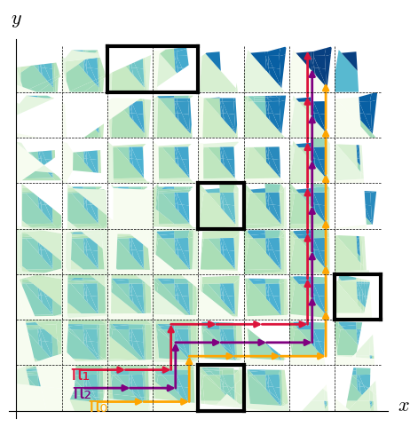
Figure 7: Paths and values for car parking ($8{\times}8$, $\beta=0.8$, partially reconstructed).

Strategy synthesis ($8{\times}8$). Fig. 8 (left) shows the perception FCP for the $8{\times}8$ environment. For this extended model, Fig. 7 (left) presents the paths from the three particles in the initial belief for the synthesised strategy, as well as lower bound values for the regions of the environment. As the figure demonstrates, the vehicle is able to reach the parking spot while avoiding the obstacles. As the full set of $\alpha$-functions is large (see Table 4), to reduce computational effort we show approximate values obtained by maximizing over a set of sampled $\alpha$-functions. Fig. 7 (right) shows how the lower and upper bound values for the initial belief change as the number of iterations of the NS-HSVI algorithm increases.

6.3 VCAS Case Study

In this case study there are two commercial aircraft: an ownship aircraft equipped with an NN-controlled vertical collision avoidance system (VCAS) and an intruder aircraft. Each second, the avoidance system gives a vertical climb-acceleration advisory $\mathit{ad}$ to the pilot of the ownship to avoid near mid-air collisions (NMACs), which occur when the aircraft are separated by less than 100 ft vertically and 500 ft horizontally. The avoidance system extends the classical VCAS [29], both by adding trust to measure uncertainty and by allowing for deviations from the advisories arising from the additional belief information. Regarding the intruder, unlike in the VCAS model of [29], we allow a non-zero constant climb-rate for the intruder. We were able to compute optimal strategies that safely guide the ownship by avoiding the collision zone.

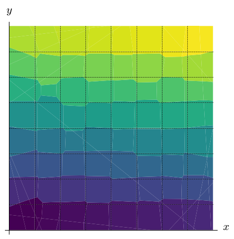
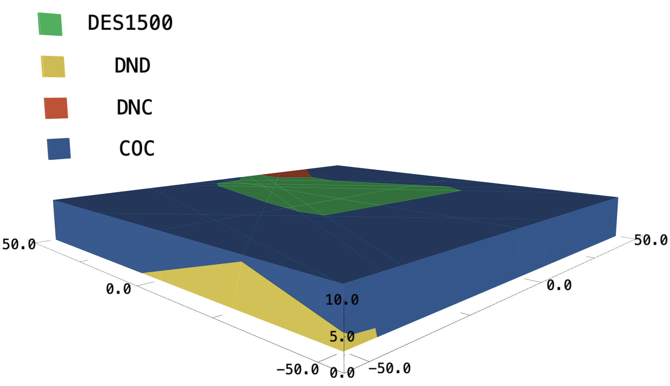
Figure 8: Perception FCP for car parking ($8{\times}8$), and a slice of the perception FCP for the COC advisory of the VCAS ($h$ scaled 10:1).

VCAS as an NS-POMDP. The input to VCAS is a tuple $(h,\dot{h}_{A},t)$, where $h$ is the relative altitude of the two aircraft, $\dot{h}_{A}$ the climb rate of ownship, and $t$ the time until the loss of horizontal separation between the aircraft. VCAS is implemented via nine feed-forward NNs, each of which outputs the scores of nine possible advisories, see Table 2. Each advisory will provide a set of acceleration values and the ownship then either accelerates at one of these values or does not accelerate. Each NN of VCAS has one hidden ReLU layer with 16 neurons, and therefore the regions in its pre-image are polytopes. If we had instead considered HorizontalCAS [43], the nonlinear environment transition function twists polytopes into non-polytopes, and would destroy our finite representations.

We model VCAS as an NS-POMDP in which the agent $\mathsf{Ag}$ is the ownship. The agent has four trust levels $\{1,\dots,4\}$, which represent the trust it has in the previous advisory. These levels increase if the current advisory is compliant with the executed action, and decrease with probability $0.5$ otherwise. A local state of the agent is of the form $(\mathit{ad}_{\mathit{pre}},\mathit{tr})$ consisting of the previous advisory and the trust level and the percept of the agent is the current VCAS advisory. An environment state is a tuple $(h,\dot{h}_{A},t)$ corresponding to the input of VCAS. Formally, we have:

• $S_{A}=\mathit{Loc}\times\mathit{Per}$ with $\mathit{Loc}=\{1,\dots,9\}\times\{1,\dots,4\}$ and $\mathit{Per}=\{1,\dots,9\}$;

• $S_{E}=[-2000,2000]\times[-50,50]\times[0,20]$;

• $\mathit{Act}=\{0,\pm 3.0,\pm 7.33,\pm 8.33,\pm 9.33,\pm 9.7,\pm 10.7,\pm 11.7\}$;

• $\Delta_{A}(\mathit{loc},\mathit{per})=\mathit{Act}$ for all $\mathit{loc}\in\mathit{Loc}$ and $\mathit{per}\in\mathit{Per}$;

• $\mathit{obs}_{A}((\mathit{ad}_{\mathit{pre}},\mathit{tr}),s_{E})=\operatorname*{argmax}(f_{\mathit{ad}_{\mathit{pre}}}(s_{E}))$, where $f_{\mathit{ad}_{\mathit{pre}}}$ is the NN associated with the previous advisory $\mathit{ad}_{\mathit{pre}}$ and the boundary point is resolved by assigning the advisory with the smallest label in Table 2;

• for $s_{A}=((\mathit{ad}_{\mathit{pre}},\mathit{tr}),\mathit{ad})\in S_{A}$, $(\mathit{ad}^{\prime},\mathit{tr}^{\prime})\in\mathit{Loc}$ and $a\in\mathit{Act}$, if $a$ is compliant with $\mathit{ad}$ (see Table 2), then:

  $$\delta_{A}(s_{A},a)((\mathit{tr}^{\prime},\mathit{ad}^{\prime}))=\left\{\begin{array}[]{cl}1&\mbox{if $(\mathit{tr}\leq 3)\wedge(\mathit{tr}^{\prime}=\mathit{tr}+1)\wedge(\mathit{ad}^{\prime}=\mathit{ad})$}\\ 1&\mbox{if $(\mathit{tr}=4)\wedge(\mathit{tr}^{\prime}=\mathit{tr})\wedge(\mathit{ad}^{\prime}=\mathit{ad})$}\\ 0&\mbox{otherwise}\end{array}\right.$$

  if $a$ is not compliant with $\mathit{ad}$, then:

  $$\delta_{A}(s_{A},a)((\mathit{tr}^{\prime},\mathit{ad}^{\prime}))=\left\{\begin{array}[]{cl}0.5&\mbox{if $(\mathit{tr}\geq 2)\wedge(\mathit{tr}^{\prime}=\mathit{tr}-1)\wedge(\mathit{ad}^{\prime}=\mathit{ad})$}\\ 0.5&\mbox{if $(\mathit{tr}\geq 2)\wedge(\mathit{tr}^{\prime}=\mathit{tr})\wedge(\mathit{ad}^{\prime}=\mathit{ad})$}\\ 1&\mbox{if $(\mathit{tr}=1)\wedge(\mathit{tr}^{\prime}=\mathit{tr})\wedge(\mathit{ad}^{\prime}=\mathit{ad})$}\\ 0&\mbox{otherwise;}\end{array}\right.$$

• for $s=(h,\dot{h}_{A},t),s^{\prime}=(h^{\prime},\dot{h}_{A}^{\prime},t^{\prime})\in S$ if

  $$\begin{array}[]{rcl}h^{\prime\prime}&=&h-\Delta t(\dot{h}_{A}-\dot{h}_{\textup{int}})-0.5\Delta t^{2}\ddot{h}_{A}\\ \dot{h}_{A}^{\prime\prime}&=&\dot{h}_{A}+\ddot{h}_{A}\Delta t\\ t^{\prime\prime}&=&t-\Delta t\end{array}$$

  then

  $$\delta_{E}(s,a)(s^{\prime})=\left\{\begin{array}[]{cl}1&\mbox{if $(h^{\prime\prime},\dot{h}_{A}^{\prime\prime},t^{\prime\prime})\in S_{E}$ and $s^{\prime}=(h^{\prime\prime},\dot{h}_{A}^{\prime\prime},t^{\prime\prime})$}\\ 1&\mbox{if $(h^{\prime\prime},\dot{h}_{A}^{\prime\prime},t^{\prime\prime})\not\in S_{E}$ and $s^{\prime}=s$}\\ 0&\mbox{otherwise}\\ \end{array}\right.$$

  where $\Delta t=1.0$ is the time step and the intruder is assumed to be a constant climb-rate $\dot{h}_{\text{int}}=30$.

Label	Advisory	Description	Actions
$(ad_{i})$			$\textup{ft/s}^{2}$
1	COC	Clear of Conflict	$-3$, $0$, $+3$
2	DNC	Do Not Climb	$-9.33$, $-8.33$, $-7.33$
3	DND	Do Not Descend	$+7.33$, $+8.33$, $+9.33$
4	DES1500	Descend at least 1500 ft/min	$-9.33$, $-8.33$, $-7.33$
5	CL1500	Climb at least 1500 ft/min	$+7.33$, $+8.33$, $+9.33$
6	SDES1500	Strengthen Descend to at least 1500 ft/min	$-11.7$, $-10.7$, $-9.7$
7	SCL1500	Strengthen Climb to at least 1500 ft/min	$+9.7$, $+10.7$, $+11.7$
8	SDES2500	Strengthen Descend to at least 2500 ft/min	$-11.7$, $-10.7$, $-9.7$
9	SCL2500	Strengthen Climb to at least 2500 ft/min	$+9.7$, $+10.7$, $+11.7$

Table 2: Available/suggested actions for each advisory of VCAS [4].

In the reward structure we consider, all action rewards are zero and the state reward function is such that for any $s\in S$: $r_{S}(s)=-1000$ if $t\in[0,1]\wedge h\in[-100,100]$ and $0$ otherwise, i.e., there is a negative reward if altitudes of the aircraft are within 100 ft at time 0 or 1. The accuracy $\varepsilon$ is $10^{-1}$.

Strategy synthesis. To compute the perception FCP $\Phi_{P}$, i.e., the preimages of the NNs for this case study, we first trained these NNs. This involved computing an MDP table policy using local approximate value iteration, reformatting this into training data and training the NNs [44]. To generate the pre-images, we adapted the method of [30], which was used to compute exact pre-images for the NNs of HorizontalCAS [43]. For example, the pre-image for the COC (Clear of Conflict) advisory is shown in Fig. 8 (right), which shows VCAS next issuing the advisory DES1500 (Descend at least 1500 ft/min) for the environment states in the green region to avoid an NMAC given the small values of $h$ and $t$.

Fig. 9 shows the paths from the four particles in the initial belief of a synthesized strategy for the VCAS case study. For the particles that would reach the collision zone at time 0 or 1 (coloured green in Fig. 9), there is a course correction that enables the ownship to narrowly escape a collision.

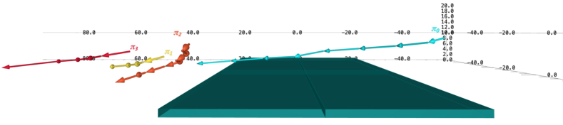
Figure 9: Paths from synthesised safe strategies for VCAS ($h$ scaled 5:1).

6.4 Performance Analysis

To conclude the experimental analysis, we first discuss the performance of the implementation based on the statistics for two case studies, and then compare the performance of particle-based and region-based beliefs, and against SARSOP.

Model	Belief type	Initial	Discount	Pts./vol.	Iter.	Comput.
		pts./regions	factor	updated		time(s)
Car parking (no obstacles, $4{\times}4$)	Particle-based	3	0.8	205	15	32.7
		5	0.8	392	11	36.3
	Region-based	1	0.8	7.6	15	99.1
Car parking (w/ obstacle, $4{\times}4$)	Particle-based	3	0.8	210	17	46.2
		5	0.8	390	15	41.9
	Region-based	1	0.8	7.6	8	80.4
Car parking (w/ obstacles, $8{\times}8$)	Particle-based	3	0.8	960	174	1820
		5	0.8	1600	119	1337
	Region-based	1	0.8	43.2	59	2075
VCAS (3 actions)	Particle-based	4	0.75	441	40	228.2
		5	0.75	649	43	475.6
		6	0.75	476	23	1467
	Region-based	1	0.75	4725	10	994.6
VCAS (15 actions)	Particle-based	4	0.75	259	11	183.7
		5	0.75	425	15	357.7
		6	0.75	228	6	127.4
	Region-based	1	0.75	4059	7	2419

Table 3: Statistics for a set of NS-POMDP solution instances.

Experimental results. The experimental results reported in this section were generated on a 2.10GHz Intel Xeon Gold. Our NS-HSVI implementation is able to compute values and strategies for particle-based and region-based instances of the models we considered in less than 1 hour (Table 3). In the table, we report the model we consider, the belief type, the number of initial points or regions, the discount factor ($\beta$), the number of updated points or the volume of the updated regions (depending on the belief type), and the overall number of iterations of Algorithm 3 as well as the time taken until convergence. We found that the branching factor of the environment transition function, the number of agent states and actions, and the number of polyhedra in the perception FCP $\Phi_{P}$ can all have a significant impact on the computation time. Table 3 shows that computation for region-based beliefs normally takes longer because the number of regions of the perception FCP $\Phi_{P}$ over which the algorithm puts positive probabilities is usually larger, and thus it requires more ISPP backups. Moreover, while the update for particle-based beliefs only involves simple operations, updating region-based beliefs is far more complex due to the need of the polyhedra image computations, intersections and volume calculations.

Figure 10: Solution times for different discount factors (for particle-based beliefs).

Another crucial aspect is the choice of the discount factor ($\beta$). Fig. 10 shows how verification times vary for the different case studies as a function of that parameter. As expected, the trend we are able to observe is that it takes longer for the algorithm to converge as the value of $\beta$ increases. The small drop in the curve for the $8\times 8$ version of the car parking example for the lower values of $\beta$ can be explained by the inherent nondeterminism of HSVI exploration, especially in the early stages of the computation when many regions may have the same lower and upper bounds. This may lead to the algorithm being indifferent with respect to the actions it takes, and thus constructing paths that have lower impact on the values of the initial belief. Finally, another element that impacts the running time is the choice of the initial belief and the model’s dynamics. This can be especially noticed when comparing the two instances of VCAS. The beliefs for the version with 15 actions have lower values for $t$ and are thus much closer to the boundaries of the environment, which considerably limits the number of reachable states and makes it possible for the algorithm to converge more quickly despite the higher number of actions.

Model	Belief type	Total regions	Lower	Upper	Strat.	Following	Avg.
	#initial	($\alpha$-functions)	bound	bound	time (s)	ratio	trust
Car parking (no obstacles, $4{\times}4$)	PB, 3	80,494	2389.3309	2389.3333	19.3	88%	3.6
	PB, 5	42,224	2047.9989	2048.0000	14.0	100%	3.9
	RB, 1	36,467	2047.9992	2048.0000	50.0	100%	3.9
Car parking (w/ obstacle, $4{\times}4$)	PB, 3	99,513	2218.6653	2218.6666	24.5	78%	3.3
	PB, 5	47,719	2047.9990	2048.0000	14.2	100%	3.9
	RB, 1	35,751	2047.9988	2048.0000	39.4	100%	3.9
Car parking (w/ obstacles, $8{\times}8$)	PB, 3	1,410,799	343.5969	343.5974	338.9	85%	4.3
	PB, 5	547,753	343.5970	343.5974	158.4	97%	4.4
	RB, 1	550,685	343.5964	343.5974	473.8	80%	4.3
VCAS (3 actions)	PB, 4	154,009	-1.2281	0.0	75.3	-	-
	PB, 5	278,447	-1.2398	0.0	127.5	-	-
	PB, 6	868,257	-0.2498	0.0	400.8	-	-
	RB, 1	22,919	-0.0715	0.0	65.5	-	-
VCAS (15 actions)	PB, 4	32,387	-0.6718	0.0	18.7	33%	1.3
	PB, 5	30,003	-0.9874	0.0	21.7	0%	1.0
	PB, 6	19,218	-1.0789	0.0	13.0	33%	1.3
	RB, 1	21,102	-0.6133	0.0	49.9	0%	1.0

Table 4: Further statistics for a set of NS-POMDP solution instances.

Table 4 shows, for a number of instances of both case studies and for each belief type, particle-based (PB) and region-based (RB): the total number of polyhedra that make up the $\alpha$-functions computed, the lower and upper bounds on values for the initial belief and the time required for strategy synthesis, i.e., reading $\alpha$-functions, finding maximum actions and updating beliefs. We also show the compliance ratio with respect to the suggested actions as well as average trust values over 20 paths generated from the synthesised strategies.

For the car parking case study (recall the accuracy is $10^{-3}$), in general, the more iterations that are needed for convergence, the higher the number of $\alpha$-functions generated and consequently the total number of regions. Strategy synthesis for region-based beliefs tends to be comparatively slower due to the complexity of the mathematical operations involved. The following ratio and average trust values are both high for this case study as the suggested actions in Table 1 are close to the optimal strategies.

Regarding VCAS, the statistics in Table 4 are for the accuracy of $10^{-1}$. The $\alpha$-functions generally have a large number of regions, as the perception FCP for each of the 9 NNs of VCAS has many regions, and hence many intersections. In addition, we note that, for this model, the following ratio and average trust values are low, and in fact have been omitted for the model with 3 actions. This is because (see Table 2) the number of suggested actions associated to each advisory is only a fraction of the 15 actions we considered and, for a given belief, there are many strategies that can lead to the optimal value. Recall also that it is assumed that the intruder aircraft is always climbing and the beliefs we considered were all reasonably close to the collision zone. We analysed the synthesised strategies and found that, in many cases, the agent chose actions that would at first lead to a faster descent than those suggested in Table 2, but then compensated by descending less, or not at all, at later stages. While the values of the actions differed, all strategies we observed led to the ownship lowering its altitude, which would lead to an increase of the overall height difference so as to escape a potential collision. Thus, the low following ratios do not reflect an inadequacy of the advisories.

Figure 11: Comparison between particle-based and region-based values.

Performance comparison. Finally, we compare values obtained for particle-based and region-based initial beliefs where the initial region covers the particles, after they have been disturbed by shifting their position along a sampled direction. This models a realistic scenario, in which the actual initial belief differs from the initial belief used to compute offline lower and upper bound functions, for example due to measurement imprecision. For a range of disturbance sizes (the distances by which the particles are shifted), the lower bound values for the average of 100 sampled points are presented in Fig. 11. The results show that, in all cases, the region-based belief values are greater than or equal to the particle-based values, and therefore the region-based approach is more robust to disturbance (i.e., generates lower bound values closer to the optimum).

As the number of reachable states for a given number of transitions from an initial particle-based belief is finite, we also compare the robustness of values obtained with our particle-based NS-HSVI and the finite-state POMDP solver SARSOP, for the $4\times 4$ dynamic vehicle parking without obstacles in Fig. 12. For an initial particle-based belief, we build two finite-state POMDPs by unrolling the model’s execution when considering $4$ and $6$ transitions, respectively. Note that no new distinct states can be reached for paths whose length exceeds $6$ in this example, as any cell in the grid can be reached from any other cell in $6$ steps. Then, we compute the value function, represented as a set of $\alpha$-vectors, for each finite-state POMDP with SARSOP. Using the value function, we approximate the values of beliefs disturbed by shifting as above, in which each shifted particle takes the value of the closest point in the finite-state space of the unrolled POMDP. The optimal value of each shifted belief is computed by unrolling from the shifted belief for a maximum of $6$ transitions and solving the resulting finite-state POMDP with SARSOP.

Figure 12: Comparison between particle-based and SARSOP values.

SARSOP performs better with respect to the computational time taken, which is understandable as SARSOP takes as input a discretised version of the model and does not operate over a continuous abstraction, as NS-HSVI does, requiring expensive operations over polyhedra. Nevertheless, the results shown in Fig. 12 demonstrate that the values achieved by strategies generated using SARSOP highly depend on how much of the model’s execution we are able to construct beforehand, as the impact of missing reward-critical states with a shorter horizon can be considerable. It also shows that particle-based NS-HSVI obtains greater or equal lower bound values compared to SARSOP within a small disturbance range. This is due to the fact that, when performing the ISPP backup, we update not only the values for the visited points but also for the regions that contain them. The optimal values of the shifted beliefs indicate that the values of the particle-based NS-HSVI and SARSOP are both valid lower bounds.

7 Conclusions

We have introduced NS-POMDPs, the first partially observable neuro-symbolic model for an agent operating in continuous state space and perceiving the environment using NNs. Motivated by the need for safety guarantees for such systems, we focus on optimal policy synthesis with discounting. By placing mild assumptions on the structure of NS-POMDPs, we are able to exploit their structure to approximate the value function from below and above using a representation of PWC $\alpha$-functions and belief-value induced functions. Using NS-HSVI, a variant of the classical HSVI algorithm, we synthesised optimal strategies for an agent parking a car and safe strategies for an agent using an aircraft collision avoidance system, employing the popular particle-based and novel region-based beliefs. Our main achievement is demonstrating the practicality of the methodology for small systems with realistic neural network components. To make progress in this challenging problem domain, similarly to other POMDP approaches, we initially focus on discounted objectives, and aim to later extend to the more complex undiscounted case (which is already undecidable for finite-state POMDPs). However, as the case studies demonstrate, we can use our approach to synthesise strategies that can then be shown to be safe in terms of provably avoiding “unsafe” parts of the state space. Further work includes efficiency improvement by incorporating sampling, adapting NS-HSVI to more general perception NNs and extending the approach to multi-agent systems.

Acknowledgements. This project was funded by the ERC under the European Union’s Horizon 2020 research and innovation programme (FUN2MODEL, grant agreement No.834115).

Appendix A Proofs from Section 4

Before we give the proofs of Section 4 we require the following definition.

Definition 9

For FCPs $\Phi_{1}$ and $\Phi_{2}$ of S, we denote by $\Phi_{1}+\Phi_{2}$ the smallest FCP of $S$ such that $\Phi_{1}+\Phi_{2}$ is a refinement of both $\Phi_{1}$ and $\Phi_{2}$, which can be computed by all combinations of intersections between regions in $\Phi_{1}$ and $\Phi_{2}$.

Lemma 1 (Perception FCP)

There exists a smallest FCP of $S$, called the perception FCP, denoted $\Phi_{P}$, such that all states in any $\phi\in\Phi_{P}$ are observationally equivalent, i.e., if $(s_{A},s_{E}),(s_{A}^{\prime},s_{E}^{\prime})\in\phi$, then $s_{A}=s_{A}^{\prime}$ and we let $s_{A}^{\phi}=s_{A}$.

Proof

Since $\mathit{obs}_{A}$ is PWC and $S_{A}$ is finite, using Definition 1 we have that for any $s_{A}=(\mathit{loc},\mathit{per})\in S_{A}$ the set $S_{E}^{s_{A}}=\{s_{E}\in S_{E}\mid\mathit{obs}_{A}(\mathit{loc},s_{E})=\mathit{per}\}$ can be expressed as a number of disjoint regions of $S_{E}$ and we let $\Phi_{E}^{s_{A}}$ be such a representation that minimises the number of such regions. It then follows that $\{\{(s_{A},s_{E})\mid s_{E}\in\phi_{E}\}\mid\phi_{E}\in\Phi_{E}^{s_{A}}\wedge s_{A}\in S_{A}\}$ is a smallest FCP of $S$ such that all states in any region are observationally equivalent. $\square$

Theorem 1 (P-PWLC closure and convergence)

If $V\in\mathbb{F}(S_{B})$ and P-PWLC, then so is $[TV]$. If $V^{0}\in\mathbb{F}(S_{B})$ and P-PWLC, then the sequence $(V^{t})_{t=0}^{\infty}$, such that $V^{t+1}=[TV^{t}]$ are P-PWLC and converges to $V^{\star}$.

Proof

Consider any $V\in\mathbb{F}(S_{B})$ that is P-PWLC, by Definition 6 there exists a finite set $\Gamma\subseteq\mathbb{F}_{C}(S)$ such that:

$$V(s_{A},b_{E})=\max\nolimits_{\alpha\in\Gamma}\langle\alpha,(s_{A},b_{E})\rangle\;\mbox{for all $(s_{A},b_{E})\in S_{B}$.}$$ (18)

Now consider any $(s_{A},b_{E}),(s_{A}^{\prime},b_{E}^{\prime})\in S_{B}$ where $s_{A}^{\prime}=(\mathit{loc}^{\prime},\mathit{per}^{\prime})$ and action $a\in\Delta_{A}(s_{A})$, and letting $P_{1}\coloneqq P(s_{A}^{\prime}\mid(s_{A},b_{E}),a)$, by (18) we have:

$$\!\!\!\!\!\!\!V(s_{A}^{\prime},b_{E}^{s_{A},a,s_{A}^{\prime}})\;=\;\max_{\alpha\in\Gamma}\langle\alpha,(s_{A}^{\prime},b_{E}^{s_{A},a,s_{A}^{\prime}})\rangle$$

$$\!\!\!\!\!\!\!\!\!\!=\max_{\alpha\in\Gamma}\int_{s_{E}^{\prime}\in S_{E}}\alpha(s_{A}^{\prime},s_{E}^{\prime})b_{E}^{s_{A},a,s_{A}^{\prime}}(s_{E}^{\prime})\textup{d}s_{E}^{\prime}$$ by (5)

$$\!\!\!\!\!\!\!\!\!\!=\max_{\alpha\in\Gamma}\int_{s_{E}^{\prime}\in S_{E}}\alpha(s_{A}^{\prime},s_{E}^{\prime})\frac{P((s_{A}^{\prime},s_{E}^{\prime})\mid(s_{A},b_{E}),a)}{P(s_{A}^{\prime}\mid(s_{A},b_{E}),a)}\textup{d}s_{E}^{\prime}$$ by (1)

$$\!\!\!\!\!\!\!\!\!\!=\max_{\alpha\in\Gamma}\int_{s_{E}^{\prime}\in S_{E}}\alpha(s_{A}^{\prime},s_{E}^{\prime})\frac{P((s_{A}^{\prime},s_{E}^{\prime})\mid(s_{A},b_{E}),a)}{P_{1}}\textup{d}s_{E}^{\prime} P_{1}$$ by definition of

$$=\frac{1}{P_{1}}\max_{\alpha\in\Gamma}\int_{s_{E}^{\prime}\in S_{E}}\alpha(s_{A}^{\prime},s_{E}^{\prime})P((s_{A}^{\prime},s_{E}^{\prime})\mid(s_{A},b_{E}),a)\textup{d}s_{E}^{\prime}$$ rearranging

$$\;=\frac{1}{P_{1}}\max_{\alpha\in\Gamma}\int_{s_{E}^{\prime}\in S_{E}}\!\!\!\!\!\!\!\!\alpha(s_{A}^{\prime},s_{E}^{\prime})\delta_{A}(s_{A},a)(\mathit{loc}^{\prime})\left(\int_{s_{E}^{\prime}\in S_{E}^{s_{A}^{\prime}}\wedge s_{E}\in S_{E}}\!\!\!\!\!\!\!\!\!\!\!\!\!\!\!\!\!\!\!\!\!\!b_{E}(s_{E})\delta_{E}(s_{E},a)(s_{E}^{\prime})\textup{d}s_{E}\right)\textup{d}s_{E}^{\prime}$$

by (3)

$$\;=\frac{1}{P_{1}}\max_{\alpha\in\Gamma}\int_{s_{E}\in E}\left(\delta_{A}(s_{A},a)(\mathit{loc}^{\prime})\int_{s_{E}^{\prime}\in S_{E}^{s_{A}^{\prime}}}\!\!\alpha(s_{A}^{\prime},s_{E}^{\prime})\delta_{E}(s_{E},a)(s_{E}^{\prime})\textup{d}s_{E}^{\prime}\right)b_{E}(s_{E})\textup{d}s_{E}$$

rearranging. (19)

Next, for any $\alpha\in\mathbb{F}_{C}(S)$, $s_{A}^{\prime}\in S_{A}$ and $a\in\mathit{Act}$ we let $\alpha^{a,s_{A}^{\prime}}:S\rightarrow\mathbb{R}$ be the function where for any $(s_{A},s_{E})\in S$ if $a\in\Delta_{A}(s_{A})$, then:

$$\alpha^{a,s_{A}^{\prime}}(s_{A},s_{E})=\delta_{A}(s_{A},a)(\mathit{loc}^{\prime})\left(\int_{s_{E}^{\prime}\in S_{E}^{s_{\vstretch{.75}{\hstretch{.75}{A}}}^{\prime}}}\alpha(s_{A}^{\prime},s_{E}^{\prime})\delta_{E}(s_{E},a)(s_{E}^{\prime})\textup{d}s_{E}^{\prime}\right)$$

$$\;=\delta_{A}(s_{A},a)(\mathit{loc}^{\prime})\left(\mbox{$\sum_{s_{E}^{\prime}\in\Theta_{s_{\vstretch{.75}{\hstretch{.75}{E}}}}^{a}\cap S_{E}^{s_{\vstretch{.75}{\hstretch{.75}{A}}}^{\prime}}}$}\alpha(s_{A}^{\prime},s_{E}^{\prime})\delta_{E}(s_{E},a)(s_{E}^{\prime})\right)$$ rearranging (20)

and otherwise $\alpha^{a,s_{A}^{\prime}}(s_{A},s_{E})=L$. Now combining (19) and (20) we have:

$$\!\!\!V(s_{A}^{\prime},b_{E}^{s_{A},a,s_{A}^{\prime}})=\frac{1}{P(s_{A}^{\prime}\mid(s_{A},b_{E}),a)}\max_{\alpha\in\Gamma}\int_{s_{E}\in E}\alpha^{a,s_{A}^{\prime}}(s_{A},s_{E})b_{E}(s_{E})\textup{d}s_{E}\,.$$ (21)

We next prove that $\alpha^{a,s_{A}^{\prime}}$ is PWC, i.e., $\alpha^{a,s_{A}^{\prime}}\in\mathbb{F}_{C}(S)$. Since $\alpha\in\mathbb{F}_{C}(S)$ there exists an FCP $\Phi$ of $S$ such that $\alpha$ is constant in each region of $\Phi$. According to Assumption 1, there exists a preimage FCP $\Phi^{\prime}$ of $\Phi+\Phi_{P}$ for action $a$, where $\Phi_{P}$ is the perception FCP from Lemma 1. Consider any region $\phi^{\prime}\in\Phi^{\prime}$ and let $\phi$ be any region of $\Phi+\Phi_{P}$ such that $\Theta_{s}^{a}\cap\phi\neq\varnothing$ for all $s\in\phi^{\prime}$. Since $\Phi_{P}$ is the perception FCP, there exists $s_{A}^{\prime}\in S_{A}$ such that if $s^{\prime}\in\phi$, then $s^{\prime}=(s_{A}^{\prime},s_{E}^{\prime})$ for some $s_{E}^{\prime}\in S_{E}$ and let $\phi_{E}=\{s_{E}\in S_{E}\mid(s_{A}^{\prime},s_{E})\in\phi\}$. If $s,\tilde{s}\in\phi^{\prime}$ such that $s=(s_{A},s_{E})$ and $\tilde{s}=(\tilde{s}_{A},\tilde{s}_{E})$, then using Assumption 1 we have $\sum_{s^{\prime}\in\Theta_{s}^{a}\cap\phi}\delta(s,a)(s^{\prime})=\sum_{\tilde{s}^{\prime}\in\Theta_{\tilde{s}}^{a}\cap\phi}\delta(\tilde{s},a)(\tilde{s}^{\prime})$ and $s_{A}=\tilde{s}_{A}$. Now combining this fact with Definition 2, it follows that:

$$\delta_{A}(s_{A},a)(\mathit{loc}^{\prime})\left(\mbox{$\sum_{s_{E}^{\prime}\in\Theta_{s_{\vstretch{.75}{\hstretch{.75}{E}}}}^{a}\cap\phi_{E}}$}\delta_{E}(s_{E},a)(s_{E}^{\prime})\right)$$

$$=\delta_{A}(\tilde{s}_{A},a)(\mathit{loc}^{\prime})\left(\mbox{$\sum_{\tilde{s}_{E}^{\prime}\in\Theta_{\tilde{s}_{\vstretch{.75}{\hstretch{.75}{E}}}}^{a}\cap\phi_{E}}$}\delta_{E}(\tilde{s}_{E},a)(\tilde{s}_{E}^{\prime})\right)\,.$$

Furthermore, since $\alpha(s_{A}^{\prime},s_{E}^{\prime})=\alpha(s_{A}^{\prime},\tilde{s}^{\prime}_{E})$ for any $(s_{A}^{\prime},s_{E}^{\prime}),(s_{A}^{\prime},\tilde{s}^{\prime}_{E})\in\phi$ and $S_{E}^{s_{A}^{\prime}}=\{s_{E}\in S_{E}\mid\mathit{obs}_{A}(\mathit{loc}^{\prime},s_{E})=\mathit{per}^{\prime}\}$ is equal to $\{\phi_{E}\mid\phi\in\Phi^{s_{A}^{\prime}}\}$ for some finite set of regions $\Phi^{s_{A}^{\prime}}\subseteq\Phi+\Phi_{P}$, it follows that $\alpha^{a,s_{A}^{\prime}}(s)=\alpha^{a,s_{A}^{\prime}}(\tilde{s})$, implying that $\alpha^{a,s_{A}^{\prime}}$ is constant in each region of $\Phi^{\prime}$.

Now substituting (21) into Definition 4 it follows that $[TV](s_{A},b_{E})$ equals:

$$\max_{a\in\Delta_{A}(s_{A})}\left\{\langle R_{a},(s_{A},b_{E})\rangle+\beta\mbox{$\sum\nolimits_{s_{A}^{\prime}\in S_{A}}$}\max_{\alpha\in\Gamma}\int_{s_{E}\in E}\alpha^{a,s_{A}^{\prime}}(s_{A},s_{E})b_{E}(s_{E})\textup{d}s_{E}\right\}$$

$$=\;\max_{a\in\Delta_{A}(s_{A})}\left\{\langle R_{a},(s_{A},b_{E})\rangle+\beta\mbox{$\sum\nolimits_{s_{A}^{\prime}\in S_{A}}$}\max_{\alpha\in\Gamma}\langle\alpha^{a,s_{A}^{\prime}},(s_{A},b_{E})\rangle\right\}$$ by (5).

Therefore letting $\Gamma^{a,s_{A}^{\prime}}=\{\alpha^{a,s_{A}^{\prime}}\mid\alpha\in\Gamma\}$ and

$$\alpha_{b_{E}}^{a,s_{A}^{\prime}}\in\arg\max\nolimits_{\alpha^{a,s_{\vstretch{.75}{\hstretch{.75}{A}}}^{\prime}}\in\Gamma^{a,s_{\vstretch{.75}{\hstretch{.75}{A}}}^{\prime}}}\langle\alpha^{a,s_{A}^{\prime}},(s_{A},b_{E})\rangle$$

where $\alpha_{b_{E}}^{a,s_{A}^{\prime}}$ is independent of $s_{A}$ due to (20), it then follows from Definition 4 that:

$$[TV](s_{A},b_{E})= \max_{a\in\Delta_{A}(s_{A})}\left\{\langle R_{a},(s_{A},b_{E})\rangle+\beta\mbox{$\sum_{s_{A}^{\prime}\in S_{A}}$}\langle\alpha^{a,s_{A}^{\prime}}_{b_{E}},(s_{A},b_{E})\rangle\right\}$$

$$= \max_{a\in\Delta_{A}(s_{A})}\left\langle R_{a}+\beta\mbox{$\sum_{s_{A}^{\prime}\in S_{A}}$}\alpha^{a,s_{A}^{\prime}}_{b_{E}},(s_{A},b_{E})\right\rangle$$ by (5). (22)

Furthermore, we have that

$$\Gamma_{(s_{A},b_{E})}=\left\{R_{a}+\beta\mbox{$\sum_{s_{A}^{\prime}\in S_{A}}$}\alpha^{a,s_{A}^{\prime}}_{b_{E}}\mid a\in\Delta_{A}(s_{A})\right\}$$

and from (22):

$$[TV](s_{A},b_{E})=\max\nolimits_{\alpha\in\Gamma_{(s_{\vstretch{.75}{\hstretch{.75}{A}}},b_{\vstretch{.75}{\hstretch{.75}{E}}})}}\langle\alpha,(s_{A},b_{E})\rangle\,.$$

Finally, since $S_{A}$, $\mathit{Act}$ and $\Gamma$ are finite, $R_{a}$ is PWC by Assumption 2 and $\alpha^{a,s_{A}^{\prime}}$ is PWC, defining $\Gamma^{\prime}$ to be the set containing the PWC functions:

$$R_{a}+\beta\mbox{$\sum_{s_{A}^{\prime}\in S_{A}}$}\alpha^{a,s_{A}^{\prime}}\in\mathbb{F}_{C}(S)$$

for all $a\in\mathit{Act}$, $s_{A}^{\prime}\in S_{A}$ and $\alpha^{a,s_{A}^{\prime}}\in\Gamma^{a,s_{A}^{\prime}}$, we have for any $(s_{A},b_{E})\in S_{B}$:

$$[TV](s_{A},b_{E})=\max\nolimits_{\alpha\in\Gamma^{\prime}}\langle\alpha,(s_{A},b_{E})\rangle.$$

Therefore, $[TV]$ is P-PWLC. As can be seen $|\Gamma^{\prime}|=|\mathit{Act}||\Gamma|^{|S_{A}|}$, and hence the number of $\alpha$-functions representing $[TV]$ given grows exponentially in the number of agent states for those representing $V$.

The remainder of the proof follows from Banach’s fixed point theorem and the fact we have proved that if $V\in\mathbb{F}(S_{B})$ and P-PWLC, so is $[TV]$. $\square$

Theorem 2 (Convexity and continuity)

For any $s_{A}\in S_{A}$, the value function $V^{\star}(s_{A},\cdot):\mathbb{P}(S_{E})\rightarrow\mathbb{R}$ is convex and for any $b_{E},b_{E}^{\prime}\in\mathbb{P}(S_{E})$:

$$|V^{\star}(s_{A},b_{E})-V^{\star}(s_{A},b_{E}^{\prime})|\leq K(b_{E},b_{E}^{\prime})$$ (23)

where $K(b_{E},b_{E}^{\prime})=(U-L)\int_{s_{E}\in S_{E}^{b_{\vstretch{.75}{\hstretch{.75}{E}}}>b_{\vstretch{.75}{\hstretch{.75}{E}}}^{\vstretch{.75}{\hstretch{.75}{{}^{\prime}}}}}}(b_{E}(s_{E})-b_{E}^{\prime}(s_{E}))\textup{d}s_{E}$ and $S_{E}^{b_{E}>b_{E}^{\prime}}=\{s_{E}\in S_{E}^{s_{A}}\mid b_{E}(s_{E})-b_{E}^{\prime}(s_{E})>0\}$.

Proof

According to Theorem 1 there exists a (possibly infinite) set $\Gamma\subseteq\mathbb{F}_{C}(S)$ such that for any $(s_{A},b_{E})\in S_{B}$:

$$V^{\star}(s_{A},b_{E})=\sup\nolimits_{\alpha\in\Gamma}\langle\alpha,(s_{A},b_{E})\rangle\,.$$ (24)

Given $s_{A}\in S_{A}$, consider any $b_{E},b_{E}^{\prime}\in\mathbb{P}(S_{E})$ and $\lambda\in[0,1]$, and we have:

$$\lambda V^{\star}(s_{A},b_{E})+(1-\lambda)V^{\star}(s_{A},b_{E}^{\prime})$$

$$=\;\lambda\sup\nolimits_{\alpha\in\Gamma}\langle\alpha,(s_{A},b_{E})\rangle+(1-\lambda)\sup\nolimits_{\alpha\in\Gamma}\langle\alpha,(s_{A},b_{E}^{\prime})\rangle$$ by (24)

$$=\;\sup\nolimits_{\alpha\in\Gamma}\langle\alpha,(s_{A},\lambda b_{E})\rangle+\sup\nolimits_{\alpha\in\Gamma}\langle\alpha,(s_{A},(1-\lambda)b_{E}^{\prime})\rangle$$ by (5)

$$\geq\;\sup\nolimits_{\alpha\in\Gamma}\langle\alpha,(s_{A},\lambda b_{E}+(1-\lambda)b_{E}^{\prime})\rangle$$ rearranging

$$=\;V^{\star}(s_{A},\lambda b_{E}+(1-\lambda)b_{E}^{\prime})$$ by (24)

which proves that $V^{\star}(s_{A},\cdot)$ is convex.

Next given $\alpha$ and $s_{A}$, let $V_{\alpha,s_{A}}(b_{E})\coloneqq\langle\alpha,(s_{A},b_{E})\rangle$ for $(s_{A},b_{E})\in S_{B}$. For any $(s_{A},b_{E}),(s_{A},b_{E}^{\prime})\in S_{B}$, without loss of generality, we can assume that $V_{\alpha,s_{A}}(b_{E})\geq V_{\alpha,s_{A}}(b_{E}^{\prime})$, and therefore:

$$|V_{\alpha,s_{A}}(b_{E})-V_{\alpha,s_{A}}(b_{E}^{\prime})|=V_{\alpha,s_{A}}(b_{E})-V_{\alpha,s_{A}}(b_{E}^{\prime})$$

$$=\langle\alpha,(s_{A},b_{E})\rangle-\langle\alpha(s_{A},b_{E}^{\prime})\rangle V_{\alpha,s_{A}}$$ by definition of

$$=\int_{s_{E}\in S_{E}^{s_{A}}}\alpha(s_{A},s_{E})b_{E}(s_{E})\textup{d}s_{E}-\int_{s_{E}\in S_{E}^{s_{A}}}\alpha(s_{A},s_{E})b^{\prime}_{E}(s_{E})\textup{d}s_{E}$$ by (5)

$$=\int_{s_{E}\in S_{E}^{s_{A}}}\alpha(s_{A},s_{E})(b_{E}(s_{E})-b_{E}^{\prime}(s_{E}))\textup{d}s_{E}$$ rearranging. (25)

Since $b_{E},b_{E}^{\prime}\in\mathbb{P}(S_{E})$ and $(s_{A},b_{E}),(s_{A},b_{E}^{\prime})\in S_{B}$, we have:

$$\int_{s_{E}\in S_{E}^{s_{A}}}b_{E}(s_{E})\textup{d}s_{E}=\int_{s_{E}\in S_{E}^{s_{A}}}b_{E}^{\prime}(s_{E})\textup{d}s_{E}=1\,.$$ (26)

Now, letting $S_{E}^{+}=\{s_{E}\in S_{E}^{s_{A}}\mid b_{E}(s_{E})-b_{E}^{\prime}(s_{E})>0\}$ and $S_{E}^{-}=\{s_{E}\in S_{E}^{s_{A}}\mid b_{E}(s_{E})-b_{E}^{\prime}(s_{E})\leq 0\}$, rearranging (26) and using the fact that $S_{E}^{+}\cup S_{E}^{-}=S_{E}^{s_{A}}$ it follows that:

$$\int_{s_{E}\in S_{E}^{-}}(b_{E}(s_{E})-b_{E}^{\prime}(s_{E}))\textup{d}s_{E}=-\int_{s_{E}\in S_{E}^{+}}(b_{E}(s_{E})-b_{E}^{\prime}(s_{E}))\textup{d}s_{E}.$$ (27)

Next, using (25), the definition of $V_{\alpha,s_{A}}$ and (5), it follows that $|V_{\alpha,s_{A}}(b_{E})-V_{\alpha,s_{A}}(b_{E}^{\prime})|$ equals:

$$\!\!\!\!\!\int_{s_{E}\in S_{E}^{+}}\!\!\alpha(s_{A},s_{E})(b_{E}(s_{E})-b_{E}^{\prime}(s_{E}))\textup{d}s_{E}+\int_{s_{E}\in S_{E}^{-}}\!\!\alpha(s_{A},s_{E})(b_{E}(s_{E})-b_{E}^{\prime}(s_{E}))\textup{d}s_{E}$$

$$\leq\int_{s_{E}\in S_{E}^{+}}U(b_{E}(s_{E})-b_{E}^{\prime}(s_{E}))\textup{d}s_{E}+\int_{s_{E}\in S_{E}^{-}}L(b_{E}(s_{E})-b_{E}^{\prime}(s_{E}))\textup{d}s_{E}$$

by definition of $$S_{E}^{+} S_{E}^{-} U L$$, , and

$$=U\int_{s_{E}\in S_{E}^{+}}(b_{E}(s_{E})-b_{E}^{\prime}(s_{E}))\textup{d}s_{E}-L\int_{s_{E}\in S_{E}^{+}}(b_{E}(s_{E})-b_{E}^{\prime}(s_{E}))\textup{d}s_{E}$$

rearranging and using (27)

$$=k\int_{s_{E}\in S_{E}^{+}}(b_{E}(s_{E})-b_{E}^{\prime}(s_{E}))\textup{d}s_{E} k=U-L$$ rearranging and letting . (28)

We can now derive the following upper bound for $V^{\star}(s_{A},b_{E})$:

$$V^{\star}(s_{A},b_{E})=\sup\nolimits_{\alpha\in\Gamma}\langle\alpha,(s_{A},b_{E})\rangle$$ by (24)

$$=\sup_{\alpha\in\Gamma}V_{\alpha,s_{A}}(b_{E}) V_{\alpha,s_{A}}$$ by definition of

$$=\sup_{\alpha\in\Gamma}(V_{\alpha,s_{A}}(b_{E}^{\prime})+V_{\alpha,s_{A}}(b_{E})-V_{\alpha,s_{A}}(b_{E}^{\prime}))$$ rearranging

$$=\sup_{\alpha\in\Gamma}(V_{\alpha,s_{A}}(b_{E}^{\prime})+|V_{\alpha,s_{A}}(b_{E})-V_{\alpha,s_{A}}(b_{E}^{\prime})|)$$ rearranging

$$\leq\sup_{\alpha\in\Gamma}\left\{V_{\alpha,s_{A}}(b^{\prime}_{E})+k\int_{s_{E}\in S_{E}^{+}}\!\!\!\!\!\!(b_{E}(s_{E})-b_{E}^{\prime}(s_{E}))\textup{d}s_{E}\right\}$$ by (28)

$$=\sup_{\alpha\in\Gamma}(V_{\alpha,s_{A}}(b^{\prime}_{E}))+k\int_{s_{E}\in S_{E}^{+}}\!\!\!\!\!\!(b_{E}(s_{E})-b_{E}^{\prime}(s_{E}))\textup{d}s_{E}$$ rearranging

$$=\sup_{\alpha\in\Gamma}\langle\alpha,(s_{A},b^{\prime}_{E})\rangle+k\int_{s_{E}\in S_{E}^{+}}\!\!\!\!\!\!(b_{E}(s_{E})-b_{E}^{\prime}(s_{E}))\textup{d}s_{E} V_{\alpha,s_{A}}$$ by definition of

$$=V^{\star}(s_{A},b_{E}^{\prime})+k\int_{s_{E}\in S_{E}^{+}}\!\!\!\!\!\!(b_{E}(s_{E})-b_{E}^{\prime}(s_{E}))\textup{d}s_{E} \mbox{by (\ref{eq:V-star-sup})}.$$

Using similar steps we can also show:

$$V^{\star}(s_{A},b^{\prime}_{E})\leq V^{\star}(s_{A},b_{E})+k\int_{s_{E}\in S_{E}^{+}}\!\!\!\!\!\!(b_{E}(s_{E})-b_{E}^{\prime}(s_{E}))\textup{d}s_{E}$$

and therefore the second part of the theorem follows. $\square$

Appendix B Proofs from Section 5

Lemma 2 (Lower bound)

At belief $(s_{A},b_{E})\in S_{B}$, the function $\alpha^{\star}$ generated by Algorithm 1 is a PWC $\alpha$-function satisfying (11), $V_{\mathit{LB}}^{\Gamma}\leq V_{\mathit{LB}}^{\Gamma^{\prime}}\leq V^{\star}$ and $V_{\mathit{LB}}^{\Gamma^{\prime}}(s_{A},b_{E})\geq[TV_{\mathit{LB}}^{\Gamma}](s_{A},b_{E})$.

Proof

By following the proof of Theorem 1 and how $\bar{a}$ and $\alpha^{s_{A}^{\prime}}$ are constructed for all $s_{A}^{\prime}\in S_{A}$, we can easily verify that $\alpha^{\star}$ in Algorithm 1 is a PWC $\alpha$-functions that satisfies (11).

For any $V_{1},V_{2}\in\mathbb{F}(S_{B})$, we use the shorthand $V_{1}\leq V_{2}$ to denote that $V_{1}(\hat{s}_{A},\hat{b}_{E})\leq V_{2}(\hat{s}_{A},\hat{b}_{E})$ for all $(\hat{s}_{A},\hat{b}_{E})\in S_{B}$. Now, in the case of the lower bound consider any $V_{\mathit{LB}}^{\Gamma}$ such that $V_{\mathit{LB}}^{\Gamma}\leq V^{\star}$. Since $\Gamma^{\prime}=\Gamma\cup\{\alpha^{\star}\}$ after updating $V_{\mathit{LB}}^{\Gamma}$ at $(s_{A},b_{E})$ through Algorithm 1, for any $(\hat{s}_{A},\hat{b}_{E})\in S_{B}$:

$$\max\nolimits_{\alpha\in\Gamma}\langle\alpha,(\hat{s}_{A},\hat{b}_{E})\rangle\leq\max\nolimits_{\alpha\in\Gamma^{\prime}}\langle\alpha,(\hat{s}_{A},\hat{b}_{E})\rangle\,.$$

Therefore combining this with the fact that $V_{\mathit{LB}}^{\Gamma}$ is a P-PWLC function for the finite set $\Gamma$, see Definition 6, we have $V_{\mathit{LB}}^{\Gamma}(\hat{s}_{A},\hat{b}_{E})\leq V_{\mathit{LB}}^{\Gamma^{\prime}}(\hat{s}_{A},\hat{b}_{E})$ and since $(\hat{s}_{A},\hat{b}_{E})$ was arbitrary $V_{\mathit{LB}}^{\Gamma}\leq V_{\mathit{LB}}^{\Gamma^{\prime}}$.

Next, again using the fact $V_{\mathit{LB}}^{\Gamma}$ is a P-PWLC function for the finite set $\Gamma$ we have:

$$V_{\mathit{LB}}^{\Gamma^{\prime}}(s_{A},b_{E}) =\max\nolimits_{\alpha\in\Gamma^{\prime}}\langle\alpha,(s_{A},b_{E})\rangle$$

$$\geq\langle\alpha^{\star},(s_{A},b_{E})\rangle$$ rearranging

$$=[TV_{\mathit{LB}}^{\Gamma}](s_{A},b_{E}) \mbox{by \eqref{eq:update-lb-condition}}.$$

In Algorithm 1, if the backup at line 6 is executed, then the Bellman operator is applied for some states in $\phi$ which may result in non-optimal Bellman backup for the other states in $\phi$, and if the backup at line 7 is executed, $\alpha^{\star}$ is assigned the lower bound $L$ in $\phi$. Therefore we have for any $(\hat{s}_{A},\hat{b}_{E})\in S_{B}$:

$$\langle\alpha^{\star},(\hat{s}_{A},\hat{b}_{E})\rangle \leq[TV_{\mathit{LB}}^{\Gamma}](\hat{s}_{A},\hat{b}_{E})$$

$$\leq[TV^{\star}](\hat{s}_{A},\hat{b}_{E}) V_{\mathit{LB}}^{\Gamma}\leq V^{\star}$$ since

$$=V^{\star}(\hat{s}_{A},\hat{b}_{E})$$ by Theorem 1. (29)

Combining this inequality with $V_{\mathit{LB}}^{\Gamma}\leq V^{\star}$, we have $V_{\mathit{LB}}^{\Gamma^{\prime}}\leq V^{\star}$ as required. $\square$

Lemma 3 (ISPP backup)

The FCP $\Phi_{\textup{product}}$ returned by Algorithm 2 is a constant-FCP of $\phi$ for $\alpha^{\star}$ and the region-by-region backup for $\alpha^{*}$ satisfies (12).

Proof

For the PWC $\alpha$-functions in the input of Algorithm 2, let $\Phi=\sum_{s_{A}^{\prime}\in\bar{S}_{A}}\Phi_{s_{A}^{\prime}}$, where $\Phi_{s_{A}^{\prime}}$ is an FCP of $S$ for $\alpha^{s_{A}^{\prime}}$.

According to Assumption 1, there exists a preimage-FCP of $\Phi$ for action $\bar{a}$. Through the image, split, preimage and product operations of Algorithm 2, all the states in any region $\phi^{\prime}\in\Phi_{\textup{product}}$ have the same reward and reach the same regions of $\Phi$. Since each $\alpha$-function $\alpha^{s_{A}^{\prime}}$ is constant over each region in $\Phi$, all states in $\phi^{\prime}$ have the same backup value from $\alpha^{s_{A}^{\prime}}$ for $s_{A}^{\prime}\in\bar{S}_{A}$. This implies that $\Phi_{\textup{product}}$ is a preimage FCP of $\Phi$ for action $\bar{a}$. Since the value backup (12) is used for each region in $\Phi_{\textup{product}}$ and the image is from the region $\phi$, then $\Phi_{\textup{product}}$ is a constant-FCP of $\phi$ for $\alpha^{\star}$, and thus the value backup (12) for $\alpha^{\star}$ is achieved by considering the regions of $\Phi_{\textup{product}}$. $\square$

Lemma 4 (Upper bound)

Given belief $(s_{A},b_{E})\in S_{B}$, if $p^{\star}=[TV_{\mathit{UB}}^{\Upsilon}](s_{A},b_{E})$, then $p^{\star}$ is an upper bound of $V^{\star}$ at $(s_{A},b_{E})$, i.e., $p^{\star}\geq V^{\star}(s_{A},b_{E})$, and if $\Upsilon^{\prime}=\Upsilon\cup\{((s_{A},b_{E}),p^{\star})\}$, then $V_{\mathit{UB}}^{\Upsilon}\geq V_{\mathit{UB}}^{\Upsilon^{\prime}}\geq V^{\star}$ and $V_{\mathit{UB}}^{\Upsilon^{\prime}}(s_{A},b_{E})\leq[TV_{\mathit{UB}}^{\Upsilon}](s_{A},b_{E})$.

Proof

Consider an upper bound $V_{\mathit{UB}}^{\Upsilon}$ such that $V_{\mathit{UB}}^{\Upsilon}\geq V^{\star}$. By construction, each pair $((s_{A}^{i},b_{E}^{i}),y_{i})$ in $\Upsilon$ satisfies $V^{\star}(s_{A}^{i},b_{E}^{i})\leq y_{i}$.

Now suppose for belief $(s_{A},b_{E})\in S_{B}$ we let $p^{\star}=[TV_{\mathit{UB}}^{\Upsilon}](s_{A},b_{E})$ and $\Upsilon^{\prime}=\Upsilon\cup\{((s_{A},b_{E}),p^{\star})\}$. The new upper bound $V_{\mathit{UB}}^{\Upsilon^{\prime}}$ after updating $V_{\mathit{UB}}^{\Upsilon}$ at $(s_{A},b_{E})$ through Algorithm 1, satisfies $V_{\mathit{UB}}^{\Upsilon}\geq V_{\mathit{UB}}^{\Upsilon^{\prime}}$ by (9). By construction of $p^{\star}$ we have:

$$p^{\star} =[TV_{\mathit{UB}}^{\Upsilon}](s_{A},b_{E})$$

$$\geq[TV^{\star}](s_{A},b_{E}) V_{\mathit{UB}}^{\Upsilon}\geq V^{\star}$$ since

$$=V^{\star}(s_{A},b_{E})$$ by Theorem 1.

Next we have:

$$V_{\mathit{UB}}^{\Upsilon^{\prime}}(s_{A},b_{E}) \leq p^{\star} ((s_{A},b_{E}),p^{\star})\in\Upsilon^{\prime}$$ since and (9)

$$=[TV_{\mathit{UB}}^{\Upsilon}](s_{A},b_{E}) p^{\star}$$ by construction of .

It therefore remains to prove the last part, i.e. that $V_{\mathit{UB}}^{\Upsilon^{\prime}}\geq V^{\star}$. Now for any $(s_{A}^{\prime},b_{E}^{\prime})\in S_{B}$, if $s_{A}^{\prime}\neq s_{A}$, then using the fact that $\Upsilon^{\prime}=\Upsilon\cup\{((s_{A},b_{E}),p^{\star})\}$ and (9) we have:

$$V_{\mathit{UB}}^{\Upsilon^{\prime}}(s_{A}^{\prime},b_{E}^{\prime}) =V_{\mathit{UB}}^{\Upsilon}(s_{A}^{\prime},b_{E}^{\prime})$$

$$\geq V^{\star}(s_{A}^{\prime},b_{E}^{\prime}) V_{\mathit{UB}}^{\Upsilon}\geq V^{\star}$$ since .

On the other hand, if $s_{A}^{\prime}=s_{A}$, then using (9) there exists $\langle\hat{\lambda}_{i}\rangle_{i\in I_{s_{\vstretch{.75}{\hstretch{.75}{A}}}}}$ with $\hat{\lambda}_{i}\geq 0$ and $\mbox{$\sum\nolimits_{i\in I_{s_{\vstretch{.75}{\hstretch{.75}{A}}}}}$}\hat{\lambda}_{i}=1$ such that:

$$V_{\mathit{UB}}^{\Upsilon^{\prime}}(s_{A}^{\prime},b_{E}^{\prime})=\mbox{$\sum\nolimits_{i\in I_{s_{\vstretch{.75}{\hstretch{.75}{A}}}}}$}\hat{\lambda}_{i}y_{i}+K_{\mathit{UB}}\left(b_{E}^{\prime},\mbox{$\sum\nolimits_{i\in I_{s_{\vstretch{.75}{\hstretch{.75}{A}}}}}$}\hat{\lambda}_{i}b_{E}^{i}\right)\,.$$ (30)

Now using Theorem 2 we have:

$$V^{\star}(s_{A}^{\prime},b_{E}^{\prime})\leq V^{\star}(s_{A},\mbox{$\sum\nolimits_{i\in I_{s_{\vstretch{.75}{\hstretch{.75}{A}}}}}$}\hat{\lambda}_{i}b_{E}^{i})+K\left(b_{E}^{\prime},\mbox{$\sum\nolimits_{i\in I_{s_{\vstretch{.75}{\hstretch{.75}{A}}}}}$}\hat{\lambda}_{i}b_{E}^{i}\right)$$

$$\leq\mbox{$\sum\nolimits_{i\in I_{s_{\vstretch{.75}{\hstretch{.75}{A}}}}}$}\hat{\lambda}_{i}V^{\star}(s_{A},b_{E}^{i})+K\left(b_{E}^{\prime},\mbox{$\sum\nolimits_{i\in I_{s_{\vstretch{.75}{\hstretch{.75}{A}}}}}$}\hat{\lambda}_{i}b_{E}^{i}\right) V^{\star} S_{B}$$ since is convex in

$$\leq\mbox{$\sum\nolimits_{i\in I_{s_{\vstretch{.75}{\hstretch{.75}{A}}}}}$}\hat{\lambda}_{i}V^{\star}(s_{A},b_{E}^{i})+K_{\mathit{UB}}\left(b_{E}^{\prime},\mbox{$\sum\nolimits_{i\in I_{s_{\vstretch{.75}{\hstretch{.75}{A}}}}}$}\hat{\lambda}_{i}b_{E}^{i}\right)$$ by (10)

$$\leq\mbox{$\sum\nolimits_{i\in I_{s_{\vstretch{.75}{\hstretch{.75}{A}}}}}$}\hat{\lambda}_{i}y_{i}+K_{\mathit{UB}}\left(b_{E}^{\prime},\mbox{$\sum\nolimits_{i\in I_{s_{\vstretch{.75}{\hstretch{.75}{A}}}}}$}\hat{\lambda}_{i}b_{E}^{i}\right) i\in I_{s_{\vstretch{.75}{\hstretch{.75}{A}}}} ((s_{A},b_{E}^{i}),y_{i})\in\Upsilon$$ since if , then

$$=V_{\mathit{UB}}^{\Upsilon^{\prime}}(s_{A}^{\prime},b_{E}^{\prime})$$ by (30).

Therefore since these are the only cases to consider for $(s_{A}^{\prime},b_{E}^{\prime})\in S_{B}$ we have $V_{\mathit{UB}}^{\Upsilon^{\prime}}\geq V^{\star}$ as required. $\square$

Lemma 5 (LP for upper bound)

The function $K_{\mathit{UB}}$ from (17) satisfies (10), and for particle-based belief $(s_{A},b_{E})$ represented by $\{(s_{E}^{i},w_{i})\}_{i=1}^{N_{b}}$, we have that $V_{\mathit{UB}}^{\Upsilon}(s_{A},b_{E})$ is the optimal value of the LP:

$$\begin{array}[]{rl}\textup{minimize:}&\sum_{k\in I_{s_{\vstretch{.75}{\hstretch{.75}{A}}}}}\lambda_{k}y_{k}+(U-L)N_{b}c\\ \textup{subject to:}&c\geq|w_{i}-\sum_{k\in I_{s_{\vstretch{.75}{\hstretch{.75}{A}}}}}\lambda_{k}P(s_{E}^{i};b_{E}^{k})|\textup{ for }1\leq i\leq N_{b}\\ &\lambda_{k}\geq 0\textup{ for }k\in I_{s_{\vstretch{.75}{\hstretch{.75}{A}}}}\;\mbox{and}\;\sum_{k\in I_{s_{\vstretch{.75}{\hstretch{.75}{A}}}}}\lambda_{k}=1\,.\end{array}$$

Proof

Consider any particle-based beliefs $(s_{A},b_{E})$ and $(s_{A},b_{E}^{\prime})$ where $(s_{A},b_{E})$ is represented by the weighted particle set $\{(s_{E}^{i},w_{i})\}_{i=1}^{N_{b}}$. Recall that $S_{E}^{b_{E}>b_{E}^{\prime}}=\{s_{E}\in S_{E}^{s_{A}}\mid b_{E}(s_{E})-b_{E}^{\prime}(s_{E})>0\}$, now by definition of $K(b_{E},b_{E}^{\prime})$, see Theorem 2, we have:

$$K(b_{E},b_{E}^{\prime})=(U-L)\int_{s_{E}\in S_{E}^{b_{\vstretch{.75}{\hstretch{.75}{E}}}>b_{\vstretch{.75}{\hstretch{.75}{E}}}^{\vstretch{.75}{\hstretch{.75}{{}^{\prime}}}}}}(b_{E}(s_{E})-b_{E}^{\prime}(s_{E}))\textup{d}s_{E}$$

$$=(U-L)\int_{s_{E}\in S_{E}^{b_{\vstretch{.75}{\hstretch{.75}{E}}}>b_{\vstretch{.75}{\hstretch{.75}{E}}}^{\vstretch{.75}{\hstretch{.75}{{}^{\prime}}}}}}|b_{E}(s_{E})-b_{E}^{\prime}(s_{E})|\textup{d}s_{E} S_{E}^{b_{E}>b_{E}^{\prime}}$$ by definition of

$$\leq(U-L)\mbox{$\sum\nolimits_{i=1}^{N_{b}}$}\left|P(s_{E}^{i};b_{E})-P(s_{E}^{i};b_{E}^{\prime})\right|$$ by Definition 7

$$\leq(U-L)N_{b}\max\nolimits_{1\leq i\leq N_{b}}\left|P(s_{E}^{i};b_{E})-P(s_{E}^{i};b_{E}^{\prime})\right|$$ rearranging

$$=(U-L)N_{b}\max\nolimits_{s_{E}\in S_{E}\wedge b_{E}(s_{E})>0}\left|P(s_{E};b_{E})-P(s_{E};b_{E}^{\prime})\right|$$ rearranging

$$=K_{\mathit{UB}}(b_{E},b_{E}^{\prime})$$ by (17).

Furthermore, (17) implies $K_{\mathit{UB}}(b_{E},b_{E})=0$, and therefore $K_{\mathit{UB}}$ satisfies (10).

Next suppose $\Upsilon=\{((s_{A}^{k},b_{E}^{k}),y_{k})\mid k\in I\}$, letting $b_{E}^{\prime}=\sum_{k\in I_{s_{\vstretch{.75}{\hstretch{.75}{A}}}}}\lambda_{k}b_{E}^{k}$ and $c=\max\nolimits_{s_{E}\in S_{E}\wedge b_{E}(s_{E})>0}|P(s_{E};b_{E})-P(s_{E};b_{E}^{\prime})|$, by definition of $K_{\mathit{UB}}$, see (17), we have:

$$K_{\mathit{UB}}(b_{E},b_{E}^{\prime}) =(U-L)N_{b}\max\nolimits_{s_{E}\in S_{E}\wedge b_{E}(s_{E})>0}|P(s_{E};b_{E})-P(s_{E};b_{E}^{\prime})|$$

$$=(U-L)N_{b}c c$$ by definition of

and therefore:

$$\mbox{$\sum\nolimits_{k\in I_{s_{\vstretch{.75}{\hstretch{.75}{A}}}}}$}\lambda_{k}y_{k}+K_{\mathit{UB}}(b_{E},b_{E}^{\prime})=\mbox{$\sum\nolimits_{k\in I_{s_{\vstretch{.75}{\hstretch{.75}{A}}}}}$}\lambda_{k}y_{k}+(U-L)N_{b}c\,.$$

Furthermore, for any $1\leq i\leq N_{b}$, by definition of $c$ and since $(s_{A},b_{E})$ is represented by the weighted particle set $\{(s_{E}^{i},w_{i})\}_{i=1}^{N_{b}}$ we have:

$$c \geq\left|P(s_{E}^{i};b_{E})-P(s_{E}^{i};b_{E}^{\prime})\right|$$

$$=\left|w_{i}-P(s_{E}^{i};b_{E}^{\prime})\right| \{(s_{E}^{i},w_{i})\}_{i=1}^{N_{b}} b_{E}$$ since represents

$$=\left|w_{i}-P\left(s_{E}^{i};\mbox{$\sum_{k\in I_{s_{\vstretch{.75}{\hstretch{.75}{A}}}}}$}\lambda_{k}b_{E}^{k}\right)\right| b_{E}^{\prime}$$ by definition of .

Therefore, the optimization problem (9) can be equivalently written as the LP of Lemma 5, i.e., the optimal value is equal to $V_{\mathit{UB}}^{\Upsilon}(s_{A},b_{E})$. $\square$

Lemma 6 (Region-based belief closure)

If $\delta_{E}^{i}(\cdot,a):S_{E}\rightarrow\delta_{E}^{i}(S_{E},a)$ is piecewise differentiable and invertible from $S_{E}$ to $T\subseteq S_{E}$, and the Jacobian determinant of the inverse function, i.e., for any $s_{E}^{\prime}\in T$:

$$\textup{Jac}(s_{E}^{\prime})\coloneqq\textup{det}\left(\frac{\textup{d}\delta_{E}^{i,-1}(s_{E}^{\prime},a)}{\textup{d}s_{E}^{\prime}}\right)$$

is PWC for $a\in\mathit{Act}$ and $1\leq i\leq N_{e}$, then region-based beliefs are closed under belief updates.

Proof

Since $\delta_{E}^{i}(\cdot,a)$ is piecewise differentiable and piecewise invertible, let $\phi_{E}\subseteq S_{E}$ be a region over which $\delta_{E}^{i}(\cdot,a)$ is differentiable and invertible. Suppose that $X_{E}$ is a random variable taking values in $\phi_{E}$, and that $X_{E}$ has a continuous uniform distribution with probability density function $b_{E}$. Due to the differentiability and thus continuity of $\delta_{E}^{i}(\cdot,a)$, the image $\phi_{E}^{\prime}=\{s_{E}^{\prime}\mid s_{E}^{\prime}=\delta_{E}^{i}(s_{E},a)\wedge s_{E}\in\phi_{E}\}$ is a region in $S_{E}$. Furthermore, suppose $X_{E}^{\prime}=\delta_{E}^{i}(X_{E},a)$ is a new random variable taking values in $\phi_{E}^{\prime}$ and let $b_{E}^{\prime}$ be the probability density function for $X_{E}^{\prime}$ over $\phi_{E}^{\prime}$. We next prove that $b_{E}^{\prime}$ is a PWC uniform distribution under the given conditions.

Let $\delta_{E}^{i,-1}(\cdot,a)$ be the inverse function of $\delta_{E}^{i}(\cdot,a)$ in $\phi_{E}$. If $\phi_{1}^{\prime}\subseteq\phi_{E}^{\prime}$, letting $\phi_{1}$ be the preimage of $\phi^{\prime}_{1}$, then

$$P(X_{E}^{\prime}\in\phi_{1}^{\prime}) =P(\delta_{E}^{i}(X_{E},a)\in\phi_{1}^{\prime}) X_{E}^{\prime}=\delta_{E}^{i}(X_{E},a)$$ since

$$=\int_{s_{E}\in\phi_{1}}b_{E}(s_{E})\textup{d}s_{E} b_{E}$$ by definition of . (31)

Using the change of variables $s_{E}=\delta_{E}^{i,-1}(s_{E}^{\prime},a)$ we have that:

$$\textup{d}s_{E} =\textup{det}\left(\frac{\textup{d}\delta_{E}^{i,-1}(s_{E}^{\prime},a)}{\textup{d}s_{E}^{\prime}}\right)\textup{d}s_{E}^{\prime}$$

$$=\textup{Jac}(s_{E}^{\prime})\textup{d}s_{E}^{\prime}$$ by definition of the Jacobian determinant

and substituting this into (31) we have:

$$P(X_{E}^{\prime}\in\phi_{1}^{\prime})=\int_{s_{E}^{\prime}\in\phi_{1}^{\prime}}b_{E}(\delta_{E}^{i,-1}(s_{E}^{\prime},a))\textup{Jac}(s_{E}^{\prime})\textup{d}s_{E}^{\prime}\,.$$

Therefore we have that for any $s_{E}^{\prime}\in\phi_{1}^{\prime}$:

$$b_{E}^{\prime}(s_{E}^{\prime})=b_{E}(\delta_{E}^{i,-1}(s_{E}^{\prime},a))\textup{Jac}(s_{E}^{\prime})$$

and since $b_{E}(\delta_{E}^{i,-1}(s_{E}^{\prime},a))=b_{E}(s_{E})$ for $s_{E}\in\phi_{E}$ is constant and by construction $\textup{Jac}(s_{E}^{\prime})$ is PWC, we have that $b_{E}^{\prime}$ is PWC over $\phi_{E}^{\prime}$ as required.

We conclude that $\delta_{E}^{i}(\cdot,a)$ transforms a random variable which has a continuous uniform distribution in a region into a new random variable which has a continuous uniform distribution over finitely many regions. Therefore, region-based belief are closed under $\delta_{E}^{i}(\cdot,a)$. $\square$

Lemma 7 (Region-based belief update)

For region-based belief $(s_{A},b_{E})$ represented by $\{(\phi_{E}^{i},w_{i})\}_{i=1}^{N_{b}}$, action $a$ and observation $s_{A}^{\prime}$: $(s_{A}^{\prime},b_{E}^{\prime})$ returned by Algorithm 4 is region-based and $b_{E}^{\prime}=b_{E}^{s_{A},a,s_{A}^{\prime}}$. Furthermore, if $h:S\to\mathbb{R}$ is PWC and $\Phi_{E}$ is a constant-FCP of $S_{E}$ for $h$ at $s_{A}$, then $\langle h,(s_{A},b_{E})\rangle=\sum_{i=1}^{N_{b}}\sum_{\phi_{E}\in\Phi_{E}}h(s_{A},s_{E})w_{i}\textup{vol}(\phi_{E}^{i}\cap\phi_{E})$ where $s_{E}\in\phi_{E}$.

Proof

Consider a region-based belief $(s_{A},b_{E})$ represented by $\{(\phi_{E}^{i},w_{i})\}_{i=1}^{N_{b}}$, action $a$ and observation $s_{A}^{\prime}$ and suppose that the belief $(s_{A}^{\prime},b_{E}^{\prime})$ is returned by Algorithm 4.

Since $\delta_{E}^{i}(\cdot,a)$ is piecewise continuous by Lemma 6, then for any region $\phi_{E}\subseteq\Phi_{E}$, the image $\{\delta_{E}^{i}(s_{E},a)\mid s_{E}\in\phi_{E}\}$ can be represented as a union of regions. Furthermore, due to the invertibility of $\delta_{E}^{i}(\cdot,a)$, these regions are disjoint and the image is uniformly reached. Letting $\phi_{ij}=\{\delta_{E}^{j}(s_{E},a)\mid s_{E}\in\phi_{E}^{i}\}$, according to the belief update (4) and the belief expression in Definition 8, we have:

$$\int_{s_{E}\in S_{E}}\!\!\!\!\!\!b_{E}(s_{E})\delta_{E}(s_{E},a)(s_{E}^{\prime})\textup{d}s_{E}=\int_{s_{E}\in S_{E}}\left(\mbox{$\sum\nolimits_{i=1}^{N_{b}}$}\chi_{\phi_{E}^{i}}(s_{E})w_{i}\right)\delta_{E}(s_{E},a)(s_{E}^{\prime})\textup{d}s_{E}$$

$$=\mbox{$\sum\nolimits_{i=1}^{N_{b}}$}\left(\int_{s_{E}\in S_{E}}\chi_{\phi_{E}^{i}}(s_{E})w_{i}\delta_{E}(s_{E},a)(s_{E}^{\prime})\textup{d}s_{E}\right)$$ rearranging

$$=\mbox{$\sum\nolimits_{i=1}^{N_{b}}$}\left(\int_{s_{E}\in\phi_{E}^{i}}w_{i}\delta_{E}(s_{E},a)(s_{E}^{\prime})\textup{d}s_{E}\right) \chi_{\phi_{E}^{i}}$$ by definition of

$$=\mbox{$\sum\nolimits_{i=1}^{N_{b}}$}\left(\int_{s_{E}\in\phi_{E}^{i}}w_{i}\left(\mbox{$\sum\nolimits_{j=1}^{N_{e}}$}\chi_{\phi_{E}^{ij}}(s_{E}^{\prime})\frac{\mu_{j}}{\textup{vol}(\phi_{E}^{ij})}\textup{d}s_{E}\right)\right)$$

by definition of $$\phi_{ij}$$ and since it is uniformly reached by Lemma 6

$$=\mbox{$\sum\nolimits_{i=1}^{N_{b}}$}\mbox{$\sum\nolimits_{j=1}^{N_{e}}$}\left(\int_{s_{E}\in\phi_{E}^{i}}w_{i}\chi_{\phi_{E}^{ij}}(s_{E}^{\prime})\frac{\mu_{j}}{\textup{vol}(\phi_{E}^{ij})}\textup{d}s_{E}\right)$$ rearranging

$$=\mbox{$\sum\nolimits_{i=1}^{N_{b}}$}\mbox{$\sum\nolimits_{j=1}^{N_{e}}$}w_{i}\chi_{\phi_{E}^{ij}}(s_{E}^{\prime})\frac{\mu_{j}}{\textup{vol}(\phi_{E}^{ij})}\left(\int_{s_{E}\in\phi_{E}^{i}}\textup{d}s_{E}\right)$$ rearranging

$$=\mbox{$\sum\nolimits_{i=1}^{N_{b}}$}\mbox{$\sum\nolimits_{j=1}^{N_{e}}$}\chi_{\phi_{E}^{ij}}(s_{E}^{\prime})\frac{w_{i}\mu_{j}\textup{vol}(\phi_{E}^{i})}{\textup{vol}(\phi_{E}^{ij})}$$ by definition of vol.

Therefore, $b_{E}^{\prime}$ can be constructed by normalizing $\int_{s_{E}\in S_{E}}b_{E}(s_{E})\delta_{E}(s_{E},a)(s_{E}^{\prime})\textup{d}s_{E}$, which is a region-based belief.

Next, consider any observation $s_{A}$ and PWC $h:S\to\mathbb{R}$ where $\Phi_{E}$ is a constant-FCP of $S_{E}$ for $h$ at $s_{A}$. By (5) we have:

$$\langle h,(s_{A},b_{E})\rangle=\int_{s_{E}\in S_{E}}h(s_{A},s_{E})b_{E}(s_{E})\textup{d}s_{E}$$

$$=\int_{s_{E}\in S_{E}}h(s_{A},s_{E})\mbox{$\sum\nolimits_{i=1}^{N_{b}}$}\chi_{\phi_{E}^{i}}(s_{E})w_{i}\textup{d}s_{E}$$ by Definition 8

$$=\mbox{$\sum\nolimits_{i=1}^{N_{b}}$}\left(\int_{s_{E}\in S_{E}}h(s_{A},s_{E})\chi_{\phi_{E}^{i}}(s_{E})w_{i}\textup{d}s_{E}\right)$$ rearranging

$$=\mbox{$\sum\nolimits_{i=1}^{N_{b}}$}\mbox{$\sum\nolimits_{\phi_{E}\in\Phi_{E}}$}\left(\int_{s_{E}\in\phi_{E}}h(s_{A},s_{E})\chi_{\phi_{E}^{i}}(s_{E})w_{i}\textup{d}s_{E}\right) \Phi_{E}$$ since is an FCP

$$=\mbox{$\sum\nolimits_{i=1}^{N_{b}}$}\mbox{$\sum\nolimits_{\phi_{E}\in\Phi_{E}}$}h(s_{A},\phi_{E})\left(\int_{s_{E}\in\phi_{E}}\chi_{\phi_{E}^{i}}(s_{E})w_{i}\textup{d}s_{E}\right)$$

since $$\Phi_{E} S_{E} h s_{A}$$ is a constant-FCP of for at

$$=\mbox{$\sum\nolimits_{i=1}^{N_{b}}$}\mbox{$\sum\nolimits_{\phi_{E}\in\Phi_{E}}$}h(s_{A},\phi_{E})w_{i}\textup{vol}(\phi_{E}^{i}\cap\phi_{E})$$ by definition of vol

which completes the proof. $\square$

Lemma 8 (Region-based upper bound)

For region-based belief $(s_{A},b_{E})$ represented by $\{(\phi_{E}^{i},w_{i})\}_{i=1}^{N_{b}}$ and $\Upsilon=\{((s_{A}^{k},b_{E}^{k}),y_{k})\mid k\in I\}$, if $K_{\mathit{UB}}=K$, $(\phi_{E}^{\textup{max}},p)$ is returned by Algorithm 5, $b_{E}^{\prime}=\sum_{k\in I_{s_{\vstretch{.75}{\hstretch{.75}{A}}}}}\lambda_{k}^{\star}b_{E}^{k}$ and $\phi_{E}^{\textup{max}}\subseteq S_{E}^{b_{E}>b_{E}^{\prime}}$ where $\lambda_{k}^{\star}$ is a solution to the LP of Algorithm 5, then $p$ is an upper bound of $V_{\mathit{UB}}^{\Upsilon}$ at $(s_{A},b_{E})$. Furthermore, if $N_{b}=1$, then $p=V_{\mathit{UB}}^{\Upsilon}(s_{A},b_{E})$.

Proof

Suppose that $(s_{A},b_{E})$ is a region-based belief represented by $\{(\phi_{E}^{i},w_{i})\}_{i=1}^{N_{b}}$, $\Upsilon=\{((s_{A}^{k},b_{E}^{k}),y_{k})\mid k\in I\}$ and suppose $K_{\mathit{UB}}=K$ and $(\phi_{E}^{\textup{max}},p)$ is returned by Algorithm 5, $b_{E}^{\prime}=\sum_{k\in I_{s_{\vstretch{.75}{\hstretch{.75}{A}}}}}\lambda_{k}^{\star}b_{E}^{k}$ where $\lambda_{k}^{\star}$ is a solution to the LP of Algorithm 5 and $\phi_{E}^{\textup{max}}\subseteq S_{E}^{b_{E}>b_{E}^{\prime}}$. Furthermore for each $k\in I$ suppose that $(s_{A}^{k},b_{E}^{k})$ is a region-based belief represented by $\{(\phi_{E}^{kj},w_{kj})\}_{j=1}^{N_{b}^{k}}$.

Since $K_{\mathit{UB}}=K$, by definition of $K$ (see Theorem 2) we have:

$$K_{\mathit{UB}}(b_{E},b_{E}^{\prime})=(U-L)\int_{s_{E}\in S_{E}^{b_{\vstretch{.75}{\hstretch{.75}{E}}}>b_{\vstretch{.75}{\hstretch{.75}{E}}}^{\vstretch{.75}{\hstretch{.75}{{}^{\prime}}}}}}(b_{E}(s_{E})-b_{E}^{\prime}(s_{E}))\textup{d}s_{E}$$

$$=(U-L)\left(\int_{s_{E}\in S_{E}^{b_{\vstretch{.75}{\hstretch{.75}{E}}}>b_{\vstretch{.75}{\hstretch{.75}{E}}}^{\vstretch{.75}{\hstretch{.75}{{}^{\prime}}}}}}b_{E}(s_{E})-\int_{s_{E}\in S_{E}^{b_{\vstretch{.75}{\hstretch{.75}{E}}}>b_{\vstretch{.75}{\hstretch{.75}{E}}}^{\vstretch{.75}{\hstretch{.75}{{}^{\prime}}}}}}b_{E}^{\prime}(s_{E})\textup{d}s_{E}\right)$$ rearranging

$$\leq(U-L)\left(\int_{s_{E}\in S_{E}}b_{E}(s_{E})-\int_{s_{E}\in S_{E}^{b_{\vstretch{.75}{\hstretch{.75}{E}}}>b_{\vstretch{.75}{\hstretch{.75}{E}}}^{\vstretch{.75}{\hstretch{.75}{{}^{\prime}}}}}}b_{E}^{\prime}(s_{E})\textup{d}s_{E}\right)$$ rearranging

$$=(U-L)\left(1-\int_{s_{E}\in S_{E}^{b_{\vstretch{.75}{\hstretch{.75}{E}}}>b_{\vstretch{.75}{\hstretch{.75}{E}}}^{\vstretch{.75}{\hstretch{.75}{{}^{\prime}}}}}}b_{E}^{\prime}(s_{E})\textup{d}s_{E}\right)\qquad\qquad\quad b_{E}\in\mathbb{P}(S_{E})$$ since . (32)

Now since $\phi_{E}^{\textup{max}}\subseteq S_{E}^{b_{E}>b_{E}^{\prime}}$ we have:

$$\int_{s_{E}\in S_{E}^{b_{\vstretch{.75}{\hstretch{.75}{E}}}>b_{\vstretch{.75}{\hstretch{.75}{E}}}^{\vstretch{.75}{\hstretch{.75}{{}^{\prime}}}}}}b_{E}^{\prime}(s_{E})\textup{d}s_{E}\;\geq\;\int_{s_{E}\in\phi_{E}^{\textup{max}}}b^{\prime}(s_{E})\textup{d}s_{E}$$

$$=\int_{s_{E}\in\phi_{E}^{\textup{max}}}\left(\mbox{$\sum_{k\in I_{s_{\vstretch{.75}{\hstretch{.75}{A}}}}}$}\lambda_{k}^{\star}b_{E}^{k}(s_{E})\textup{d}s_{E}\right) b_{E}^{\prime}$$ by definition of

$$=\mbox{$\sum\nolimits_{k\in I_{s_{\vstretch{.75}{\hstretch{.75}{A}}}}}$}\left(\int_{s_{E}\in\phi_{E}^{\textup{max}}}\lambda_{k}^{\star}b_{E}^{k}(s_{E})\textup{d}s_{E}\right)$$ rearranging

$$=\mbox{$\sum\nolimits_{k\in I_{s_{\vstretch{.75}{\hstretch{.75}{A}}}}}$}\left(\int_{s_{E}\in\phi_{E}^{\textup{max}}}\lambda_{k}^{\star}\mbox{$\sum\nolimits_{j=1}^{N_{b}^{k}}$}\chi_{\phi_{E}^{kj}}(s_{E})w_{kj}\textup{d}s_{E}\right)$$

since $$\{(\phi_{E}^{kj},w_{kj})\}_{j=1}^{N_{b}^{k}} b^{k}_{E}$$ represents

$$=\mbox{$\sum\nolimits_{k\in I_{s_{\vstretch{.75}{\hstretch{.75}{A}}}}}$}\mbox{$\sum\nolimits_{j=1}^{N_{b}^{k}}$}\lambda_{k}^{\star}\left(\int_{s_{E}\in\phi_{E}^{\textup{max}}}\chi_{\phi_{E}^{kj}}(s_{E})w_{kj}\textup{d}s_{E}\right)$$ rearranging

$$=\mbox{$\sum\nolimits_{k\in I_{s_{\vstretch{.75}{\hstretch{.75}{A}}}}}$}\mbox{$\sum\nolimits_{j=1}^{N_{b}^{k}}$}\lambda_{k}^{\star}w_{kj}\textup{vol}(\phi_{E}^{kj}\cap\phi_{E}^{\textup{max}})$$ by definition of vol. (33)

Thus, substituting (33) into (32) we have:

$$K_{\mathit{UB}}(b_{E},b_{E}^{\prime})\leq(U-L)\left(1-\mbox{$\sum\nolimits_{k\in I_{s_{\vstretch{.75}{\hstretch{.75}{A}}}}}$}\mbox{$\sum\nolimits_{j=1}^{N_{b}^{k}}$}\lambda_{k}^{\star}w_{kj}\textup{vol}(\phi_{E}^{kj}\cap\phi_{E}^{\textup{max}})\right)$$

and using (9), it follows that the optimal value $p$ to the LP of Algorithm 5 is an upper bound of $V_{\mathit{UB}}^{\Upsilon}$ at $(s_{A},b_{E})$.

Finally, suppose that $N_{b}=1$. Therefore $\phi_{E}^{\textup{max}}=\phi_{E}^{1}$ and since $\phi_{E}^{1}$ is the unique region with positive probabilities for $b_{E}$, by definition of $S_{E}^{b_{E}>b_{E}^{\prime}}$ it follows that $S_{E}^{b_{E}>b_{E}^{\prime}}\subseteq\phi_{E}^{1}$. Combining these with $\phi_{E}^{\textup{max}}\subseteq S_{E}^{b_{E}>b_{E}^{\prime}}$, we have that $S_{E}^{b_{E}>b_{E}^{\prime}}=\phi_{E}^{\textup{max}}=\phi_{E}^{1}$. Therefore, all the inequalities above become equalities, and therefore $p=V_{\mathit{UB}}^{\Upsilon}(s_{A},b_{E})$. $\square$

References

- [1] J. Gupta, M. Egorov, M. Kochenderfer, Cooperative multi-agent control using deep reinforcement learning, in: Proc. AAMAS’17, Vol. 10643 of LNCS, Springer, 2017, pp. 66–83.
- [2] S. Amizadeh, H. Palangi, A. Polozov, Y. Huang, K. Koishida, Neuro-symbolic visual reasoning: Disentangling, in: Proc. ICML’20, PMLR, 2020, pp. 279–290.
- [3] S. Shalev-Shwartz, S. Shammah, A. Shashua, Safe, multi-agent, reinforcement learning for autonomous driving, arXiv:1610.03295 (2016).
- [4] M. E. Akintunde, E. Botoeva, P. Kouvaros, A. Lomuscio, Verifying Strategic Abilities of Neural-symbolic Multi-agent Systems, in: Proc. KR’20, 2020, pp. 22–32.
- [5] C. H. Papadimitriou, J. N. Tsitsiklis, The complexity of Markov decision processes, Math. Oper. Res. 12 (3) (1987) 441–450.
- [6] K. Chatterjee, M. Chmelík, R. Gupta, A. Kanodia, Optimal cost almost-sure reachability in POMDPs, Artificial Intelligence 234 (2016) 26–48.
- [7] G. Shani, J. Pineau, R. Kaplow, A survey of point-based POMDP solvers, Auton. Agents Multi-Agent Syst. 27 (1) (2013) 1–51.
- [8] J. M. Porta, N. Vlassis, M. T. Spaan, P. Poupart, Point-based value iteration for continuous POMDPs, JMLR 7 (2006) 2329–2367.
- [9] M. K. Sarker, L. Zhou, A. Eberhart, P. Hitzler, Neuro-symbolic artificial intelligence, AI Comm. (2021) 1–13.
- [10] T. Smith, R. Simmons, Heuristic search value iteration for POMDPs, in: Proc. UAI’04, AUAI, 2004, p. 520–527.
- [11] L. Burks, I. Loefgren, N. R. Ahmed, Optimal continuous state POMDP planning with semantic observations: A variational approach, IEEE Trans. Robotics 35 (6) (2019) 1488–1507.
- [12] Z. Zamani, S. Sanner, P. Poupart, K. Kersting, Symbolic dynamic programming for continuous state and observation POMDPs, Adv. Neural Inf. Process. Syst. 25 (2012).
- [13] X. Jiang, J. Yang, X. Tan, H. Xi, Observation-based optimization for POMDPs with continuous state, observation, and action spaces, IEEE Trans. Automatic Control 64 (5) (2018) 2045–2052.
- [14] S. Brechtel, T. Gindele, R. Dillmann, Solving continuous POMDPs: Value iteration with incremental learning of an efficient space representation, in: Proc. ICML’13, PMLR, 2013, pp. 370–378.
- [15] J. Van Den Berg, S. Patil, R. Alterovitz, Efficient approximate value iteration for continuous gaussian POMDPs, in: Proc. AAAI’12, Vol. 26(1), 2012, pp. 1832–1838.
- [16] M. H. Lim, C. J. Tomlin, Z. N. Sunberg, Voronoi progressive widening: Efficient online solvers for continuous state, action, and observation POMDPs, in: Proc. CDC’21, 2021, pp. 4493–4500.
- [17] T. Smith, R. Simmons, Point-based POMDP algorithms: Improved analysis and implementation, in: Proc. UA’05, AUAI, 2005, p. 542–549.
- [18] K. Horák, B. Bošanskỳ, V. Kovařík, C. Kiekintveld, Solving zero-sum one-sided partially observable stochastic games, Artificial Intelligence 316 (2023) 103838.
- [19] J. Pineau, G. Gordon, S. Thrun, et al., Point-based value iteration: An anytime algorithm for POMDPs, in: Proc. IJCAI’13, Vol. 3, 2003, pp. 1025–1032.
- [20] G. Shani, R. I. Brafman, S. E. Shimony, Forward search value iteration for pomdps., in: Proc. IJCAI’07, 2007, pp. 2619–2624.
- [21] H. Kurniawati, D. Hsu, W. S. Lee, SARSOP: Efficient point-based POMDP planning by approximating optimally reachable belief spaces., in: Robotics: Science and Systems, Vol. 4, 2008, pp. 65–72.
- [22] R. Yan, G. Santos, X. Duan, D. Parker, M. Kwiatkowska, Finite-horizon equilibria for neuro-symbolic concurrent stochastic games, in: Proc. UAI’22, Vol. 180, PMLR, 2022, pp. 2170–2180.
- [23] R. Yan, G. Santos, G. Norman, D. Parker, M. Kwiatkowska, Strategy synthesis for zero-sum neuro-symbolic concurrent stochastic games, arXiv.2202.06255 (2022).
- [24] M. Kwiatkowska, G. Norman, D. Parker, G. Santos, R. Yan, Probabilistic Model Checking for Strategic Equilibria-Based Decision Making: Advances and Challenges, in: 47th International Symposium on Mathematical Foundations of Computer Science (MFCS 2022), Vol. 241, 2022, pp. 4:1–4:22.
- [25] M. Cleaveland, L. Lindemann, R. Ivanov, G. J. Pappas, Risk verification of stochastic systems with neural network controllers, Artificial Intelligence 313 (2022) 103782.
- [26] S. Carr, N. Jansen, U. Topcu, Verifiable RNN-based policies for POMDPs under temporal logic constraints, in: Proc. IJCAI’20, 2020, pp. 4121–4127.
- [27] D. Bertsekas, Dynamic programming and optimal control: Volume I, Athena scientific, 2012.
- [28] L. P. Kaelbling, M. L. Littman, A. R. Cassandra, Planning and acting in partially observable stochastic domains, Artificial intelligence 101 (1-2) (1998) 99–134.
- [29] K. D. Julian, M. J. Kochenderfer, A reachability method for verifying dynamical systems with deep neural network controllers, arXiv.1903.00520 (2019).
- [30] K. Matoba, F. Fleuret, Computing preimages of deep neural networks with applications to safety, openreview.netforum?id=FN7BUOG78e (2020).
- [31] E. J. Sondik, The optimal control of partially observable Markov processes over the infinite horizon: Discounted costs, Oper. Res. 26 (2) (1978) 282–304.
- [32] K. Horák, B. Bošanský, K. Chatterjee, Goal-HSVI: Heuristic search value iteration for goal POMDPs, in: Proc. JCAI’18, 2018, pp. 4764–4770.
- [33] T. Smith, Probabilistic planning for robotic exploration, Carnegie Mellon University, 2007.
- [34] D. Crisan, A. Doucet, A survey of convergence results on particle filtering methods for practitioners, IEEE Transactions on Signal Processing 50 (3) (2002) 736–746.
- [35] A. Doucet, N. De Freitas, N. J. Gordon (Eds.), Sequential Monte Carlo methods in practice, Vol. 1(2), Springer, 2001.
- [36] M. Lauri, D. Hsu, J. Pajarinen, Partially observable Markov decision processes in robotics: A survey, IEEE Transactions on Robotics (2022) 1–20.
- [37] X. Ma, P. Karkus, D. Hsu, W. S. Lee, Particle filter recurrent neural networks, in: Proc. AAAI’20, Vol. 34(4), 2020, pp. 5101–5108.
- [38] A. Doucet, S. Godsill, C. Andrieu, On sequential Monte Carlo sampling methods for Bayesian filtering, Statistics and computing 10 (3) (2000) 197–208.
- [39] A. Papoulis, S. U. Pillai, Probability, random variables, and stochastic processes, Tata McGraw-Hill Education, 2002.
- [40] R. Bagnara, P. M. Hill, E. Zaffanella, The Parma Polyhedra Library: Toward a complete set of numerical abstractions for the analysis and verification of hardware and software systems, Sci. Comput. Program. 72 (1) (2008) 3–21, bugseng.com/ppl.
- [41] Gurobi Optimization, LLC, Gurobi Optimizer Reference Manual, gurobi.com (2021).
- [42] L. De Moura, N. Bjørner, Z3: An efficient SMT solver, in: Proc. TACAS’08, Vol. 4963 of LNCS, Springer, 2008, pp. 337–340, github.com/Z3Prover/z3.
- [43] K. D. Julian, M. J. Kochenderfer, Guaranteeing safety for neural network-based aircraft collision avoidance systems, in: Proc. DASC’19, IEEE, 2019, pp. 1–10, the source code is available from openreview.net/forum?id=FN7_BUOG78e.
- [44] K. D. Julian, S. Sharma, J.-B. Jeannin, M. J. Kochenderfer, Verifying aircraft collision avoidance neural networks through linear approximations of safe regions, arXiv.1903.00762The source code is available from github.com/sisl/VerticalCAS (2019).