High-order geometric integrators for the variational Gaussian approximation

Abstract

Among the single-trajectory Gaussian-based methods for solving the time-dependent Schrödinger equation, the variational Gaussian approximation is the most accurate one. In contrast to Heller’s original thawed Gaussian approximation, it is symplectic, conserves energy exactly, and may partially account for tunneling. However, the variational method is also much more expensive. To improve its efficiency, we symmetrically compose the second-order symplectic integrator of Faou and Lubich and obtain geometric integrators that can achieve an arbitrary even order of convergence in the time step. We demonstrate that the high-order integrators can speed up convergence drastically compared to the second-order algorithm and, in contrast to the popular fourth-order Runge-Kutta method, are time-reversible and conserve the norm and the symplectic structure exactly, regardless of the time step. To show that the method is not restricted to low-dimensional systems, we perform most of the analysis on a non-separable twenty-dimensional model of coupled Morse oscillators. We also show that the variational method may capture tunneling and, in general, improves accuracy over the non-variational thawed Gaussian approximation.

I Introduction

Nuclear quantum effects play an important role in many fundamental phenomena in physics and chemistry. [1, 2, 3] The idea of using Gaussian wavepackets [4, 5, 2, 6, 7, 8, 3, 9, 10] for the semiclassical description of nuclei goes back to the works of Heller [11, 12, 13] and Hagedorn. [14, 15] In addition to many convenient mathematical properties, [9] the Gaussian wavepacket is the exact solution of the Schrödinger equation in a many-dimensional harmonic potential, which is often used as a starting point for modeling and discussing molecular vibrations. The localized nature of Gaussians allows nuclear dynamics to be performed on the fly, without the need to pre-compute a full potential energy surface. As a result, the Gaussian-based methods can be easily combined [16, 17, 18] with ab initio evaluation of the potential. In addition, the Gaussian wavepackets inherit a symplectic structure from the manifold of the quantum-mechanical Hilbert space. [19, 20, 21]

Employing a superposition of Gaussian basis functions to represent the nuclear wavepacket makes it possible to address more subtle quantum effects, including interference, tunneling, diffraction, wavepacket splitting, and nonadiabatic transitions. A number of multi-trajectory Gaussian-based approaches, such as the full multiple spawning, [22, 23, 24] coupled coherent states, [25] minimum energy method, [26, 27, 28] variational multiconfigurational Gaussians, [29, 8] multiconfigurational Ehrenfest method, [30, 31] Gaussian dephasing representation, [32] initial value representation, [33] frozen Gaussian approximation, [13] Herman-Kluk propagator, [34] hybrid dynamics, [35] multiple coherent states,[36] and divide-and-conquer semiclassical dynamics[37, 38] were developed to capture these effects. However, the use of multiple coupled or uncoupled Gaussians makes these methods rather expensive and difficult to converge, especially in combination with on-the-fly ab initio simulation of large systems.

To simulate systems with weak anharmonicity and mild quantum effects, it is sometimes sufficient to use single-trajectory Gaussian-based methods. Because they avoid the issue of convergence with respect to the number of trajectories, the single-trajectory techniques preserve more geometric properties. An original method in this family is Heller’s thawed Gaussian approximation (TGA), [11, 39, 3] which propagates a single Gaussian wavepacket in the local harmonic approximation of the potential. The TGA is much more accurate than the global harmonic approximations because it at least partially includes anharmonicity. [18, 40, 41] However, because the TGA uses a classical trajectory, it cannot describe quantum tunneling. [42] Here, we explore the variational Gaussian approximation (VGA), [43, 6, 44] which evolves a single Gaussian wavepacket according to the Dirac-Frenkel-McLachlan time-dependent variational principle. [45, 46, 47, 48, 49, 6] In contrast to the TGA, the VGA conserves both the symplectic structure and energy [19, 50, 6] and, in addition, may partially capture tunneling. [51, 52]

The variational Gaussian wavepacket dynamics was introduced in the seminal work of Heller. [48] Heather and Metiu derived equations of motion for the Gaussian’s parameters using a variational “minimum error method”. [53] Coalson and Karplus [43] obtained a refined version of these equations by applying the time-dependent variational principle to a multi-dimensional Gaussian wavepacket ansatz. Poirier derived the equations of the VGA using quantum trajectories.[54] The non-canonical symplectic structure of these equations was found for a spherical Gaussian wavepacket by Faou and Lubich [19] and generalized to an arbitrary multi-dimensional Gaussian wavepacket by Ohsawa and Leok. [21] The equations of the VGA contain expectation values of the potential and its first two derivatives, which, in general, cannot be evaluated analytically. Therefore, for practical applications, the potential should be approximated,[4, 21, 55] which introduces further errors. To avoid these additional errors here, we have designed a multi-dimensional nonseparable coupled Morse oscillator potential, whose matrix elements can be computed exactly.

Faou and Lubich developed an integration method to numerically solve the equations of motion for the VGA. [19] Their integrator is symplectic, norm-conserving, time-reversible, and for sufficiently small time steps, energy-conserving. [6] It is of second-order accuracy in the time step. [6] Here, to make the VGA more practical, we make their algorithm more efficient by increasing the order of convergence using various recursive and non-recursive composition techniques. [50, 56, 57, 58, 59, 60, 61, 62, 63] We also generalize their method from a spherical to a general multi-dimensional Gaussian and demonstrate the geometric properties of the high-order integrators.

The remainder of this paper is organized as follows. After reviewing the variational Gaussian wavepacket dynamics in Sec. II, we discuss its geometric properties in Sec. III. Nearly all of these geometric properties are preserved by the symplectic integrators, which are described in Sec. IV. In Sec. V, we provide numerical examples that confirm the improved accuracy of the VGA over those of other single-trajectory Gaussian-based methods. We also use the multi-dimensional coupled Morse potential to numerically verify the convergence, geometric properties, and increased efficiency of the high-order integrators. Section VI concludes this paper.

II Variational Gaussian approximation

Assuming the validity of the Born-Oppenheimer approximation, [64, 65] the motion of the nuclei can be described by the time-dependent Schrödinger equation

$$i\hbar\,d|\Psi_{t}\rangle/dt=\hat{H}|\Psi_{t}\rangle$$ (1)

with a time-independent Hamiltonian operator

$$\hat{H}=\hat{T}+\hat{V}=T(\hat{p})+V(\hat{q})$$ (2)

where $\hat{T}\equiv T(\hat{p}):=\hat{p}^{T}\cdot m^{-1}\cdot\hat{p}/2$ is the kinetic energy, depending only on the momentum $p$, $\hat{V}\equiv V(\hat{q})$ is the potential energy, depending only on the position $q$, and $m$ is the real-symmetric mass matrix. Solving Eq. (1) in high-dimensional systems is a formidable task, and various approaches were developed to approximate the solution. [2] Among these, the VGA [43, 44] is obtained by applying the time-dependent variational principle [45, 46, 6]

$$\langle\delta\psi_{t}\,|\big{(}i\hbar\frac{d}{dt}-\hat{H}\big{)}|\,\psi_{t}\rangle=0$$ (3)

to the complex Gaussian ansatz [48]

$$\psi_{t}(q) =\text{exp}\big{\{}(i/\hbar)\big{[}(q-q_{t})^{T}\cdot A_{t}\cdot(q-q_{t})/2$$

$$+p_{t}^{T}\cdot(q-q_{t})+\gamma_{t}\big{]}\big{\}}$$ (4)

approximating the wavefunction $\Psi_{t}$. In Eq. (4), $q_{t}$ and $p_{t}$ are $D$-dimensional real vectors representing the position and momentum of the Gaussian’s center, $A_{t}=\mathcal{A}_{t}+i\mathcal{B}_{t}$ is a $D\times D$ complex symmetric matrix whose real part $\mathcal{A}_{t}$ introduces a spatial chirp and whose positive-definite imaginary part $\mathcal{B}_{t}$ determines the width of the Gaussian, and $\gamma_{t}=\phi_{t}+i\delta_{t}$ is a complex number whose real part $\phi_{t}$ introduces a time-dependent phase and whose imaginary part $\delta_{t}$ ensures normalization at all times. The squared norm of $\psi_{t}$ is

$$I(\mathcal{B}_{t},\delta_{t}):=\lVert\psi_{t}\rVert^{2}=[\text{det}({\pi\hbar}/{\mathcal{B}_{t}})]^{1/2}e^{-{2\delta_{t}}/{\hbar}}.$$ (5)

In Appendix C we show that applying the variational principle (3) to the Gaussian ansatz (4) yields the system

$$\dot{q}_{t} =m^{-1}\cdot p_{t},$$ (6)

$$\dot{p}_{t} =-V_{1},$$ (7)

$$\dot{A}_{t} =-A_{t}\cdot m^{-1}\cdot A_{t}-V_{2},$$ (8)

$$\dot{\gamma}_{t} =T(p_{t})-V_{0}+(i\hbar/2)\,\text{Tr}\big{(}m^{-1}\cdot A_{t}\big{)}$$ (9)

of ordinary differential equations for the parameters, where $T(p_{t})=p_{t}^{T}\cdot m^{-1}\cdot p_{t}/2$ and

$$V_{0}=\langle\hat{V}\rangle-\text{Tr}\big{(}{\langle\hat{V}^{\prime\prime}\rangle}\cdot\Sigma_{t}\big{)}/2,\quad V_{1}=\langle\hat{V}^{\prime}\rangle,\quad V_{2}=\langle\hat{V}^{\prime\prime}\rangle.$$ (10)

Here, $\hat{V}^{\prime}:=V^{\prime}(q)|_{q=\hat{q}}$ and $\hat{V}^{\prime\prime}:=V^{\prime\prime}(q)|_{q=\hat{q}}$ denote the gradient and Hessian of the potential energy operator and

$$\Sigma_{t}:=\langle(\hat{q}-q_{t})\otimes(\hat{q}-q_{t})^{T}\rangle=(\hbar/2)\,\mathcal{B}_{t}^{-1}$$ (11)

is the position covariance. Above and throughout this paper, we use a shorthand notation $\langle\hat{O}\rangle:=\langle\psi_{t}|\hat{O}|\psi_{t}\rangle$ for the expectation value of the operator $\hat{O}$ in the normalized state $\psi_{t}$. Since by assumption the Gaussian wavepacket retains its Gaussian form for all times, the VGA cannot describe wavepacket splitting.

Rewriting Gaussian (4) in Hagedorn’s parametrization [14, 44]

$$\psi_{t}(q) =(\pi\hbar)^{-D/4}(\text{det}\,Q_{t})^{-1/2}\text{exp}\big{\{}(i/\hbar)\big{[}(q-q_{t})^{T}\cdot$$

$$P_{t}\cdot Q_{t}^{-1}\cdot(q-q_{t})/2+p_{t}^{T}\cdot(q-q_{t})+S_{t}\big{]}\big{\}}$$ (12)

leads to equivalent, yet more classical-like equations

$$\dot{Q}_{t} =m^{-1}\cdot P_{t},$$ (13)

$$\dot{P}_{t} =-V_{2}\cdot Q_{t},$$ (14)

$$\dot{S}_{t} =T(p_{t})-V_{0}.$$ (15)

The new parameters $Q_{t}$ and $P_{t}$ are two $D\times D$ complex matrices, related to the Gaussian’s width via $A_{t}=P_{t}\cdot Q_{t}^{-1}$ and satisfying the relations

$$Q_{t}^{T}\cdot P_{t}-P_{t}^{T}\cdot Q_{t}=0,$$ (16)

$$Q_{t}^{\dagger}\cdot P_{t}-P_{t}^{\dagger}\cdot Q_{t}=2iI_{D},$$ (17)

where $I_{D}$ is the $D\times D$ identity matrix. $S_{t}$ is a real scalar generalizing the classical action. The norm of the Gaussian (12) is

$$\lVert\psi(t)\rVert=\text{det}\big{[}\text{Im}\,(P_{t}\cdot Q_{t}^{-1})\cdot Q_{t}\cdot Q_{t}^{\dagger}\big{]}^{-1/4}.$$ (18)

III Geometric properties of the VGA

If $\hat{P}(\psi_{t})$ denotes the orthogonal projection onto the tangent space at $\psi_{t}$ of the approximation manifold $M$ of complex Gaussians, the variational principle (3) is equivalent to the nonlinear Schrödinger equation [6, 66, 67]

$$i\hbar\,d|\psi_{t}\rangle/dt=\hat{H}_{\text{eff}}(\psi_{t})\,|\psi_{t}\rangle$$ (19)

with an effective, state-dependent Hamiltonian

$$\hat{H}_{\text{eff}}(\psi_{t}):=\hat{P}(\psi_{t})\,\hat{H}=\hat{T}+\hat{P}(\psi_{t})\,\hat{V}.$$ (20)

In the position representation, the effective potential $\hat{V}_{\text{eff}}(\psi_{t}):=\hat{P}(\psi_{t})\,\hat{V}$ is a quadratic function [44, 67]

$$V_{\text{eff}}(q;\psi_{t}) =V_{0}+V_{1}^{T}\cdot(q-q_{t})$$

$$\quad+(q-q_{t})^{T}\cdot V_{2}\cdot(q-q_{t})/2,$$ (21)

where $V_{0}$, $V_{1}$, and $V_{2}$ are given in Eq. (10). The time evolution operator of the effective Hamiltonian (20) is also nonlinear and can be expressed as

$$\hat{U}_{\text{eff}}(t,t_{0};\psi):=\mathcal{T}\text{exp}\bigg{[}-\frac{i}{\hbar}\int_{t_{0}}^{t}\hat{H}_{\text{eff}}({\psi_{t^{\prime}}})\,dt^{\prime}\bigg{]},$$ (22)

where $\mathcal{T}$ denotes the time-ordering operator. Next, we discuss the geometric properties of the linear Schrödinger equation that are preserved by the VGA.

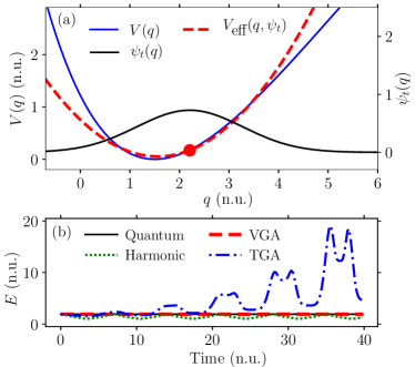
Figure 1: Energy conservation by the VGA. (a) Gaussian wavepacket $\psi_{t}$ propagated in a Morse potential $V$ using the VGA with an effective potential $V_{\textrm{eff}}$, (b) energy of the wavepacket propagated with various methods.

III.1 Energy conservation

Although a nonlinear evolution does not generally conserve energy, [66, 68] the energy is conserved in the VGA as in any other method derived from the time-dependent variational principle. [69, 43, 70, 6, 71, 72, 73, 44] To see this, note that the arbitrary infinitesimal change $\delta\psi_{t}$ in the variational principle (3) can be chosen to be proportional to $\dot{\psi}_{t}$. Therefore,

$$\dot{E} =d\langle\hat{H}\rangle/dt=2\,\text{Re}\langle\dot{\psi}_{t}|\hat{H}|\psi_{t}\rangle$$

$$=2\,\text{Re}\langle\dot{\psi}_{t}|i\hbar\,\dot{\psi}_{t}\rangle=2\,\text{Re}\big{[}i\hbar\,\lVert\dot{\psi}_{t}\rVert^{2}\big{]}=0,$$ (23)

which proves conservation of energy $E=\langle\hat{H}\rangle$.

Panel (a) of Fig. 1 shows an example of a Gaussian wavepacket propagated in a Morse potential. The effective potential $V_{\text{eff}}$ of the VGA differs from the local harmonic approximation since $V_{\text{eff}}$ is not tangent to $V$. Panel (b) compares the energies of the wavepacket propagated with various methods. Unlike the two non-variational semiclassical methods (the TGA and harmonic approximation), the VGA conserves energy exactly. Note that we use the natural units (n.u.) with $\hbar=m=1$. For other simulation details, see the supplementary material.

III.2 Effective energy conservation

The VGA also conserves the effective energy $E_{\text{eff}}=\langle\hat{H}_{\text{eff}}\rangle=\langle\hat{T}\rangle+\langle\hat{V}_{\text{eff}}\rangle$, [67] because the effective energy is equal to the energy $(\langle\hat{H}_{\text{eff}}\rangle=\langle\hat{H}\rangle)$, and the energy is conserved. The equality $\langle\hat{H}_{\text{eff}}\rangle=\langle\hat{H}\rangle$ follows because

$$\langle\hat{V}_{\text{eff}}\rangle =\langle\hat{V}\rangle-\text{Tr}\big{(}{\langle\hat{V}^{\prime\prime}\rangle}\cdot\Sigma_{t}\big{)}/2+\langle\hat{V}^{\prime}\rangle^{T}\cdot\langle\hat{q}-q_{t}\rangle$$

$$\quad+\text{Tr}[{\langle\hat{V}^{\prime\prime}\rangle}\cdot\langle(\hat{q}-q_{t})\otimes(\hat{q}-q_{t})^{T}\rangle]/2$$

$$=\langle\hat{V}\rangle.$$ (24)

III.3 Norm conservation

The manifold $M$ of unnormalized complex Gaussian wavepackets contains rays, [6, 67] i.e., for each $\psi_{t}\in M$ and each complex number $\lambda$, we have $\lambda\,\psi_{t}\in M$. Therefore, the variation $\delta\psi_{t}\propto\psi_{t}$ is permitted; invoking the variational principle (3) with $\delta\psi_{t}\propto\psi_{t}$ implies that [44]

$$d\lVert\psi_{t}\rVert^{2}/dt =2\,\text{Re}\langle\psi_{t}|\dot{\psi}_{t}\rangle=2\,\text{Re}\langle\psi_{t}|(i\hbar)^{-1}\hat{H}\psi_{t}\rangle$$

$$=2\,\text{Re}\big{[}(i\hbar)^{-1}\langle\hat{H}\rangle\big{]}=0.$$ (25)

Thus, the VGA, as well as other, more general Gaussian wavepacket methods, conserve the norm $\lVert\psi_{t}\rVert$ of the propagated Gaussian. [67, 43, 6, 44]

III.4 Non-conservation of the inner product and distance

Due to nonlinearity, the VGA generally does not conserve the inner product between states $\psi_{1}$ and $\psi_{2}$: [67]

$$d\langle\psi_{1}|\psi_{2}\rangle/dt =\langle\dot{\psi}_{1}|\psi_{2}\rangle+\langle\psi_{1}|\dot{\psi}_{2}\rangle$$

$$=(i\hbar)^{-1}\langle\psi_{1}|\hat{H}_{\text{eff}}(\psi_{1})-\hat{H}_{\text{eff}}(\psi_{2})|\psi_{2}\rangle\neq 0.$$ (26)

Although the VGA conserves the norm, the non-conservation of the inner product leads to the non-conservation of the distance between $\psi_{1}$ and $\psi_{2}$:

$$d(\psi_{1},\psi_{2}) :=\lVert\psi_{1}-\psi_{2}\rVert=\langle\psi_{1}-\psi_{2}|\psi_{1}-\psi_{2}\rangle^{1/2}$$

$$\,\,=\big{(}\lVert\psi_{1}\rVert^{2}+\lVert\psi_{2}\rVert^{2}-2\,\text{Re}\,\langle\psi_{1}|\psi_{2}\rangle\big{)}^{1/2}.$$ (27)

III.5 Time reversibility

The nonlinear evolution (22) is reversible since [66, 67]

$$\psi_{t,\text{FB}}:=\hat{U}_{\text{eff}}(t_{0},t;\psi)\hat{U}_{\text{eff}}(t,t_{0};\psi)\psi_{0}=\psi_{0},$$ (28)

where $\psi_{t,\text{FB}}$ is the state obtained by propagating the initial state $\psi_{0}$ first forward in time with the evolution operator $\hat{U}_{\text{eff}}(t,t_{0};\psi)$ and then backward in time with the reverse evolution operator

$$\hat{U}_{\text{eff}}(t_{0},t;\psi): =\tilde{\mathcal{T}}\text{exp}\bigg{[}-\frac{i}{\hbar}\int_{t}^{t_{0}}\hat{H}_{\text{eff}}({\psi_{t^{\prime}}})\,dt^{\prime}\bigg{]}$$

$$=\tilde{\mathcal{T}}\text{exp}\bigg{[}\frac{i}{\hbar}\int_{t_{0}}^{t}\hat{H}_{\text{eff}}({\psi_{t^{\prime}}})\,dt^{\prime}\bigg{]}$$

$$=\hat{U}_{\text{eff}}(t,t_{0};\psi)^{-1};$$ (29)

$\tilde{\mathcal{T}}$ is the reverse time-ordering operator.

III.6 Symplecticity

Manifold $M$ of Gaussian wavepackets can be endowed with a non-canonical symplectic structure. [50, 21] Faou and Lubich showed that the spherical Gaussian wavepacket inherits this symplectic structure from the infinite-dimensional Hilbert space manifold by the variational principle. [19] Ohsawa and Leok used the symplectic structure of this manifold to derive the variational Gaussian wavepacket dynamics as a non-canonical Hamiltonian system with the Hamiltonian function $h(q_{t},p_{t},A_{t},\gamma_{t}):=\langle\psi_{t}|\hat{H}|\psi_{t}\rangle$. [21] Employing a combination of their approaches, in Appendix C, we find the non-canonical symplectic structure of the more general non-spherical Gaussian wavepacket and rederive the equations of motion (6)-(9) for the Gaussian’s parameters.

IV Geometric integrators for the VGA

IV.1 Second-order symplectic integrator

Faou and Lubich proposed a symplectic algorithm for the numerical time integration of the differential equations of the VGA. [19, 50, 6] The integrator is based on the splitting of the Hamiltonian into the kinetic and potential energy terms. We have generalized their method for scalar mass $m$ and width $A_{t}$ to non-diagonal, symmetric matrices $m$ and $A_{t}$. [67] During the kinetic propagation $[\hat{H}_{\text{eff}}=T(\hat{p})]$, Eqs. (6)-(9) have the analytical solution

$$q_{t} =q_{0}+t\,m^{-1}\cdot p_{0},$$ (30)

$$p_{t} =p_{0},$$ (31)

$$A_{t} =(A_{0}^{-1}+t\,m^{-1})^{-1},$$ (32)

$$\gamma_{t} =\gamma_{0}+t\,T(p_{0})+(i\hbar/2)\,\text{ln}\,[\,\text{det}\,(I_{D}+t\,m^{-1}\cdot A_{0})],$$ (33)

and, during the potential propagation $[\hat{H}_{\text{eff}}=V_{\text{eff}}(\hat{q})]$, they have the analytical solution

$$q_{t} =q_{0},$$ (34)

$$p_{t} =p_{0}-t\,V_{1}(q_{0},\text{Im}\,A_{0}),$$ (35)

$$A_{t} =A_{0}-t\,V_{2}(q_{0},\text{Im}\,A_{0}),$$ (36)

$$\gamma_{t} =\gamma_{0}-t\,V_{0}(q_{0},\text{Im}\,A_{0}).$$ (37)

Applying the potential propagation for time $\Delta t/2$, kinetic propagation for time $\Delta t$, and potential propagation for time $\Delta t/2$ in sequence yields a “potential-kinetic-potential”(VTV) algorithm that is of the second order in the time step $\Delta t$. Another second-order algorithm is the “kinetic-potential-kinetic”(TVT) algorithm, which is obtained by swapping the potential and kinetic propagations in the VTV algorithm. Each of these two numerical algorithms gives the state $\psi_{t+\Delta t}$ at time $t+\Delta t$ from the state $\psi_{t}$ at time $t$:

$$|\psi_{t+\Delta t}\rangle=\hat{U}_{2}(t+\Delta t,t;\psi)|\psi_{t}\rangle,$$ (38)

where $\hat{U}_{2}$ is the approximate second-order evolution operator associated with the VTV or TVT algorithm.

In Hagedorn’s parametrization, the flow $\Phi_{\text{T},t}$ associated with the kinetic propagation is

$$q_{t} =q_{0}+t\,m^{-1}\cdot p_{0},$$ (39)

$$p_{t} =p_{0},$$ (40)

$$Q_{t} =Q_{0}+t\,m^{-1}\cdot P_{0},$$ (41)

$$P_{t} =P_{0},$$ (42)

$$S_{t} =S_{0}+t\,T(p_{0}),$$ (43)

and the potential flow $\Phi_{\text{V},t}$ is

$$q_{t} =q_{0},$$ (44)

$$p_{t} =p_{0}-t\,V_{1}(q_{0},Q_{0}),$$ (45)

$$Q_{t} =Q_{0},$$ (46)

$$P_{t} =P_{0}-t\,V_{2}(q_{0},Q_{0})\cdot Q_{0},$$ (47)

$$S_{t} =S_{0}-t\,V_{0}(q_{0},Q_{0}).$$ (48)

IV.2 High-order symplectic integrators

High-order integrators can be obtained by composing the second-order (VTV or TVT) algorithm (38). More precisely, any symmetric algorithm $\hat{U}_{p}$ of even order $p$ can generate an evolution operator $\hat{U}_{p+2}$ of order $p+2$ if it is symmetrically composed as

$$\hat{U}_{p+2}(t+\Delta t,t;\psi):=\hat{U}_{p}(t+\xi_{M}\Delta t,t+\xi_{M-1}\Delta t;\psi)\\ \quad\cdots\hat{U}_{p}(t+\xi_{1}\Delta t,t;\psi),$$ (49)

where $M$ is the total number of composition steps and $\xi_{n}:=\sum_{j=1}^{n}\gamma_{j}$ denotes the sum of the first $n$ real composition coefficients $\gamma_{j}$, which satisfy the relations $\sum_{j=1}^{M}\gamma_{j}=1$ (consistency), $\gamma_{M+1-j}=\gamma_{j}$ (symmetry), and $\sum_{j=1}^{M}\gamma_{j}^{p+1}=0$ (order increase guarantee). [50] The most common composition methods are the recursive triple-jump [57] ($M=3$) and Suzuki’s fractal [58] ($M=5$). Although both methods can generate high-order integrators, the number of composition steps grows exponentially with the order of convergence. To further increase the efficiency, we mainly use “optimal” nonrecursive methods[74, 61] to obtain integrators of sixth-, eighth-, and tenth-order. We refer to them as “optimal”composition methods because they minimize the magnitudes of composition steps defined as $\sum_{j=1}^{M}|\gamma_{j}|$ or $\max_{j}|\gamma_{j}|$. Suzuki’s fractal gives the optimal fourth-order scheme. [62] For more details on these composition schemes, see Ref. 62. We compare the efficiencies and numerically verify the predicted order of convergence of these integrators for the VGA in Sec. V and in the supplementary material.

IV.3 Geometric properties of the symplectic integrators

Each kinetic or potential step of the symplectic integrators is the exact solution of the nonlinear Schrödinger equation (19) with $\hat{H}_{\text{eff}}=\hat{T}$ or $\hat{H}_{\text{eff}}=\hat{V}_{\text{eff}}$, and thus has all the geometric properties of the VGA. All symplectic integrators that are obtained by symmetric composition of the kinetic and potential steps are time-reversible, norm-conserving, and symplectic. [19, 6, 67] However, due to the splitting, they are only approximately energy-conserving, with an error $\mathcal{O}(\Delta t^{M})$ where $M$ is greater than or equal to the order of the integrator. [19, 6, 63, 75, 67]

V Numerical examples

In what follows, we investigate the VGA and the proposed high-order integrators in different model systems. For the numerical experiments, we have specifically chosen the quartic double-well and coupled Morse potentials, for both of which the expectation values of the potential energy, gradient, and Hessian, needed in the VGA, can be computed analytically. We also compare the VGA with two other Gaussian wavepacket methods, the TGA and harmonic approximation, defined in Appendix A.

V.1 Over-the-barrier motion and tunneling in a double well

Double-well systems are ubiquitous in chemistry, physics, and biology. [76] Well-known molecular examples of double-well systems include the inversion of ammonia, phosphine, and arsine. [42] The most remarkable phenomenon in double-well potentials is the quantum tunneling, [77] which allows hopping between its two minima through a classically forbidden region. Here, we consider a one-dimensional symmetric double-well potential

$$V(q)=a-b\,q^{2}+c\,q^{4}$$ (50)

with positive $a$, $b$, and $c$. This potential is a special case of the quartic potential, described by Eq. (127) in Appendix D.1 with parameters $V(q_{\text{eq}})=a$, $V^{\prime}(q_{\text{ref}})=V^{\prime\prime\prime}(q_{\text{ref}})=0$, $V^{\prime\prime}(q_{\text{ref}})=-2\,b$, and $V^{(4)}(q_{\text{ref}})=24\,c$. The expectation values of the quartic potential, its gradient and Hessian are derived in Appendix D.1.

Figure 2 analyzes the dynamics of a wavepacket propagated in the double-well potential (50) with $a=1$, $b=5$, and $c=2.5$. The initial state was a real Gaussian with width “matrix”$A_{0}=4\,i$ and zero momentum. Depending on the initial position of the Gaussian, its energy was above or below the potential barrier. The grid for the exact quantum dynamics consisted of $512$ points between $-10$ and $10$. Time step $\Delta t=0.001$ and the second-order (TVT) symplectic integrator were used in all simulations.

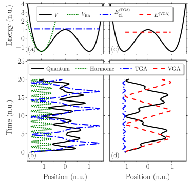
Figure 2: Thawed Gaussian approximation (TGA) can describe the classical over-the-barrier motion in double-well systems, and the variational Gaussian approximation (VGA) can also describe quantum tunneling. Panel (b) associated with panel (a) shows that the TGA with classical energy $E_{\textrm{cl}}$ above the barrier can cross the barrier, whereas the harmonic approximation with approximated harmonic potential $V_{\textrm{HA}}$ cannot. Panel (d) associated with panel (c) shows that the VGA, unlike the TGA, can even tunnel through the barrier.

The left panels of Fig. 2 show the “over-the-barrier”motion of a wavepacket with initial position $q_{0}=-1.42$ and energy $E\approx 5.36$. Panel (a) shows the double-well potential, its harmonic approximation $V_{\text{HA}}$ at the minimum of the left well, and the conserved “classical” energy $E_{\text{cl}}=p^{2}_{t}/2m+V(q_{t})\approx 1.083$ of the TGA calculated at the Gaussian’s center, which evolves according to Hamilton’s equations of motion [Eqs. (6) and (7) with coefficients (61)]. Because the classical energy is slightly above the potential barrier, the wavepacket passes the barrier, which is confirmed in panel (b) by the TGA and the exact quantum results. In contrast, the same wavepacket propagated with the harmonic approximation cannot cross the barrier because the harmonic potential confines it to the left well [see panels (a) and (b)].

Several studies [51, 52] found that the VGA may realize tunneling in double-well systems. Our results, shown in the right-hand panels of Fig. 2, confirm this observation for a wavepacket with initial position $q_{0}=-0.95$ and energy $E\approx 0.71$, which is below the potential barrier [panel (c)]. Panel (d) shows that unlike the TGA, which shows small oscillations around the minimum of the left well, the VGA captures quantum tunneling at least qualitatively, since the VGA wavepacket clearly moves back and forth between the two wells.

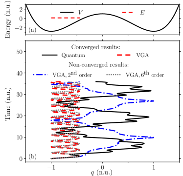
Figure 3: Failure of the VGA to detect tunneling in highly anharmonic systems and the importance of using high-order integrators. (a) The double well potential and the wavepacket’s energy. (b) The difference between the exact quantum and fully converged VGA results shows that the VGA cannot capture tunneling in this case. However, due to cancellation of errors, the numerically non-converged results of the VGA, obtained with the second-order integrator, recover the tunneling. Interestingly, with approximately the same computational effort, the sixth-order integrator calculations already agree with the fully converged VGA result.

However, sometimes the VGA can fail to capture tunneling (see Fig. 3), especially when the double well is highly anharmonic or the barrier is extremely high. Figure 3 shows the dynamics of an initially Gaussian wavepacket with $q_{0}=-1$, $p_{0}=0$, and width $A_{0}=(20/9)^{2}\,i$ in the double well (50) with parameters $a=1$, $b=7.5$, and $c=3.75$. The energy of the wavepacket, $E\sim 0.12$, is below the energy of the barrier. Comparison of the exact quantum calculation with the fully converged VGA result obtained using the sixth-order integrator with a small time step of $\Delta t=0.02$ implies that the VGA fails to capture tunneling in this system.

Let us demonstrate the importance of high-order integrators in situations at the border of tunneling and non-tunneling regimes. Panel (b) of Fig. 3 also shows less converged results of the VGA obtained by a low- and a high-order integrators. Due to the low accuracy, a simulation by the second-order integrator with a time step of $\Delta t=0.08$ and computational cost of $\sim 297.7\,\text{s}$, measured in central processing unit (CPU) time, incorrectly shows tunneling. Interestingly, even with a much larger time step of $\Delta t=0.18$ and a slightly lower computational cost of $\sim 275.4\,\text{s}$, the sixth-order integrator gives the correct results. To make the computational cost of the initialization and finalization negligible, we considered the CPU time corresponding to a longer simulation time $t=10^{4}=10000$.

V.2 Multi-dimensional coupled Morse potential

To study multi-dimensional systems without having to approximate $\langle\hat{V}\rangle$, $\langle\hat{V}^{\prime}\rangle$, and $\langle\hat{V}^{\prime\prime}\rangle$, we have designed a non-separable, arbitrary-dimensional anharmonic potential with analytical expectation values. This $D$-dimensional coupled Morse potential,

$$V(q)=V_{\text{eq}}+\sum_{j=1}^{D}\,V_{j}(q_{j})+V_{\text{cpl}}(q),$$ (51)

consists of $D$ standard one-dimensional Morse potentials $V_{j}(q_{j})$ for all its vibrational modes $q_{j}$, which are, in addition, mutually coupled with a somewhat artificial, non-separable multi-dimensional Morse coupling $V_{\text{cpl}}(q)$. In Eq. (51), $V_{\text{eq}}$ is the potential at the equilibrium position $q_{\text{eq}}$, and each one-dimensional Morse potential

$$V_{j}(q_{j}):=d_{e}^{\prime}\big{[}1-y_{j}(a_{j}^{\prime},q_{j})\big{]}^{2}$$ (52)

depends on the dissociation energy $d_{e}^{\prime}$, decay parameter $a_{j}^{\prime}$, and one-dimensional Morse variable

$$y_{j}(a_{j}^{\prime},q_{j}):=\exp\big{[}-a_{j}^{\prime}\,(q_{j}-q_{\text{eq},j})\big{]}.$$ (53)

The $D$-dimensional Morse coupling

$$V_{\text{cpl}}(q):=d_{e}\,\big{[}1-y(a,q)\big{]}^{2}$$ (54)

depends on the dissociation energy $d_{e}$, decay vector $a$, and $D$-dimensional Morse variable

$$y(a,q):=\exp\big{[}-a^{T}\cdot(q-q_{\text{eq}})\big{]}.$$ (55)

The coupling $V_{\text{cpl}}(q)$ results in non-separability. The decay parameter $a_{j}^{\prime}$, dissociation energy $d_{e}^{\prime}$, and dimensionless anharmonicity $\chi_{j}^{\prime}$ are related by the equation [78]

$$a_{j}^{\prime}=\chi_{j}^{\prime}\,\sqrt{8\,d_{e}^{\prime}},$$ (56)

and, similarly, the decay vector $a$, dissociation energy $d_{e}$, and dimensionless anharmonicity vector $\chi$ are related via

$$a=\chi\,\sqrt{8\,d_{e}}.$$ (57)

The expectation values $\langle\hat{V}\rangle$, $\langle\hat{V}^{\prime}\rangle$, and $\langle\hat{V}^{\prime\prime}\rangle$ in a Gaussian wavepacket are derived in Appendix D.2.

Next, we report the results of several simulations that demonstrate: (i) the better accuracy of the VGA over other single-trajectory Gaussian-based methods, (ii) the preservation of the geometric properties of the VGA by the symplectic integrators, and (iii) the efficiency of high-order integrators. After inspecting a low-dimensional ($2$D) system, for which the grid-based quantum calculations are available as a benchmark, we analyze the convergence and geometric properties of the symplectic integrators in a high-dimensional ($20$D) system.

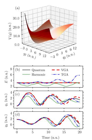
Figure 4: Dynamics of an initially Gaussian wavepacket in a two-dimensional coupled Morse potential shown in panel (a). (b) Energy. (c) and (d): Expectation values of coordinates.

Panel (a) of Fig. 4 shows a two-dimensional coupled Morse potential (51) with energy $V_{\text{eq}}=0$ at the equilibrium position $q_{\text{eq}}=(1,1)$. It is composed of two one-dimensional Morse potentials with the same dissociation energy $d_{e}^{\prime}=11.25$ and different anharmonicities $\chi_{1}^{\prime}=0.02$ and $\chi_{2}^{\prime}=0.017$. The parameters of the coupling term are $d_{e}=5.75$ and $\chi=(0.014,0.017)$. The initial state was a real Gaussian with $q_{0}=(-0.75,1.75)$, $p_{0}=(0,0)$, and a diagonal width matrix $A_{0}$ with non-zero elements $A_{0,11}=A_{0,22}=i$. This wavepacket was then propagated for $20000$ steps of $\Delta t=0.001$ with the second-order symplectic integrator. The position grid for the exact quantum dynamics consisted of $256$ points between $-3$ and $13$ in both directions.

Panel (b) of Fig. 4 indicates that the VGA conserves energy, while neither the TGA nor the harmonic approximation are energy-conserving. Panels (c) and (d) show that, for very short times, all approximate methods recover the exact quantum results, but their accuracies decrease with increasing time. However, the VGA remains accurate for longer than the TGA, which in turn remains accurate for longer than the harmonic approximation.

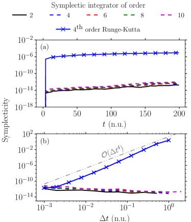
Figure 5: Conservation of the symplectic structure of the Gaussian wavepackets by the symplectic integrators and its non-conservation by the fourth-order Runge-Kutta method. The system is the same two-dimensional coupled Morse potential as in Fig. 4. The symplecticity (58) is shown: (a) as a function of time $t$ for a fixed time step $\Delta t=2^{-4}\,\textrm{n.u.}$ and (b) as a function of time step $\Delta t$ at the final time $t_{f}=200\,\textrm{n.u.}$ To avoid clutter, only the high-order symplectic integrators obtained with the optimal composition are displayed.

We also used the two-dimensional system to numerically verify the symplecticity of the integrators for the VGA. We have developed a numerical procedure to check the symplecticity of the VGA by measuring the distance

$$d\big{(}\Phi_{t}^{\prime}(z_{0})^{T}\cdot B(z_{t})\cdot\Phi_{t}^{\prime}(z_{0}),B(z_{0})\big{)}$$

$$\,\,=\lVert\Phi_{t}^{\prime}(z_{0})^{T}\cdot B(z_{t})\cdot\Phi_{t}^{\prime}(z_{0})-B(z_{0})\rVert$$ (58)

between the “initial” and “final” symplectic structure matrices $B(z_{0})$ and $B(z_{t})$. Here, vector $z_{t}$ contains components of the parameters $q_{t}$, $p_{t}$, $Q_{t}$, and $P_{t}$, $B(z_{t})$ is a skew-symmetric matrix representing the symplectic two-form of Gaussian wavepackets, [20] and $\Phi_{t}^{\prime}(z_{0})$ is the Jacobian of the VGA evolution $z_{t}=\Phi_{t}(z_{0})$. We chose to work in Hagedorn’s parametrization because the evaluation of the Jacobian is simpler and the symplectic structure matrix $B$ is independent of $z_{t}$; see Appendix C.2 for details.

Figure 5 shows the symplecticity (58) of the Gaussian wavepackets propagated with the VGA in the two-dimensional potential shown in Fig. 4(a). Although the propagation time in Fig. 5 is ten times longer than that in Fig. 4, all symplectic integrators conserve the symplectic structure as a function of both time and time step. In contrast, Fig. 5 shows that the popular fourth-order Runge-Kutta approach is not symplectic.

To show that, unlike grid-based quantum methods, the VGA is feasible in high-dimensional models, we have constructed a twenty-dimensional coupled Morse potential (51), composed of twenty Morse potentials (52) with the same dissociation energy $d_{e}^{\prime}=0.1$ and anharmonicity parameters $\chi_{j}^{\prime},\,\,j=1,\dots,20$ uniformly varying in the range between $0.001$ and $0.005$. The parameters of the coupling term are $d_{e}=0.075$ and $\chi_{j}=(3/4)\,\chi_{j}^{\prime}$. The initial Gaussian was real, had zero position and momentum and a diagonal width matrix with non-zero elements $A_{0,jj}=4\,d_{e}\chi_{j}\,i$. The wavepacket was propagated for $2^{17}=131072$ steps of $\Delta t=0.125$ with the second-order symplectic integrator.

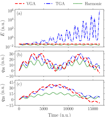
Figure 6: Dynamics of a Gaussian wavepacket propagated in a twenty-dimensional coupled Morse potential with the variational Gaussian (VGA), thawed Gaussian (TGA), and harmonic approximations. Energy [panel (a)] and displacement along two coordinates [panels (b) and (c)] are shown.

Figure 6 compares the dynamics of the Gaussian wavepacket propagated with different methods in this twenty-dimensional system. Initially, results of all methods overlap almost perfectly. However, after a short time, first the harmonic approximation and later the TGA start to deviate from the VGA.

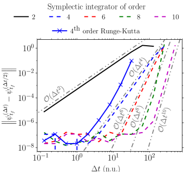
Figure 7: Convergence of the symplectic integrators and of the fourth-order Runge-Kutta method for the VGA, measured by the convergence error at the final time $t_{f}=2^{16}\,\textrm{n.u.}=65536\,\textrm{n.u.}$ as a function of the time step $\Delta t$. The convergence error is defined as the distance $d(\psi^{(\Delta t)}_{t},\psi^{(\Delta t/2)}_{t})\equiv\lVert\psi^{(\Delta t)}_{t}-\psi^{(\Delta t/2)}_{t}\rVert$, where $\psi^{(\Delta t)}_{t}$ denotes the state at time $t$ obtained after propagation with the time step $\Delta t$.

To analyze the convergence and geometric properties of the integrators, we repeated the VGA simulation with several high-order symplectic integrators and with the fourth-order Runge-Kutta method. Figure 7 compares the convergence of various methods as a function of the time step. For all methods, the obtained orders of convergence agree with the predicted ones, indicated by the gray straight lines.

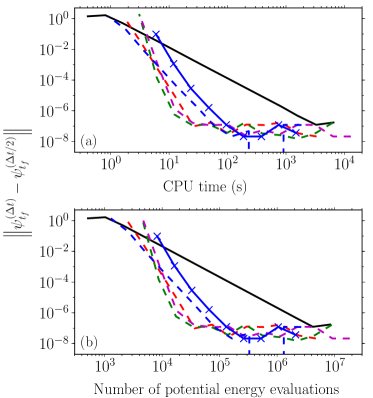
Figure 8: Efficiency of the symplectic integrators and of the fourth-order Runge-Kutta method for the VGA. The efficiency is measured by plotting the convergence error, defined in the caption of Fig. 7, as a function of (a) the computational cost (CPU time) or (b) the number of potential energy evaluations. The line labels are the same as those in Fig. 7.

Since the high-order methods require many composition substeps to be performed at each time step $\Delta t$, the higher efficiency is not guaranteed solely by a higher order of convergence. Therefore, in Fig. 8, we provide two direct ways to measure the efficiency: one plotting the convergence error as a function of the CPU time, and the other plotting the error as a function of the number of potential energy evaluations. The similarity between panels (a) and (b) confirms that the potential propagation substeps are the most time-consuming parts of the simulation. In addition, Fig. 8 shows that high-order optimal integrators are more efficient than both the second-order symplectic integrator and the fourth-order Runge-Kutta method. For example, below a rather large error of $10^{-1}$, the fourth-order symplectic integrator is already more efficient than the second-order algorithm. The efficiency gain increases when high accuracy is desired. Indeed, for a moderate error of $10^{-6}$, the eighth-order method is $100$ times faster than the second-order symplectic method and more than $5$ times faster than the fourth-order Runge-Kutta approach. The plateau indicates the machine precision error.

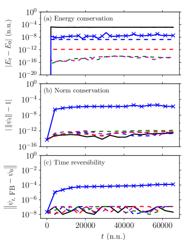
Figure 9: Geometric properties of various integrators for the VGA as a function of time $t$ for a large time step $\Delta t=8\,\textrm{n.u.}$ (a) Energy, (b) norm, and (c) time reversibility [Eq. (59)] are shown. The line labels are the same as those in Fig. 7.

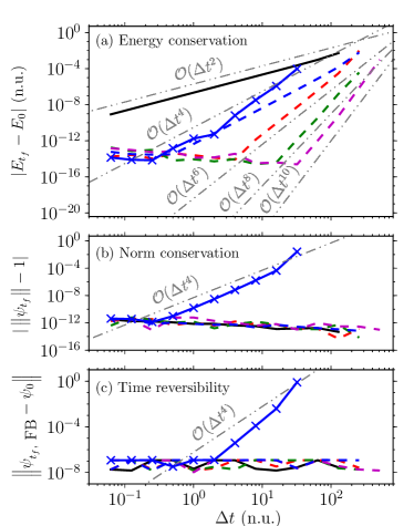
Figure 10: Geometric properties of various integrators for the VGA as a function of the time step $\Delta t$ measured at the final time $t_{f}=2^{16}\,\textrm{n.u.}=65536\,\textrm{n.u.}$ (a) Energy, (b) norm, and (c) time reversibility [Eq. (59)] are shown. The line labels are the same as those in Fig. 7.

Figure 9 shows the time dependence of energy, norm, and time reversibility, while Fig. 10 shows how these geometric properties depend on the time step. To analyze the conservation of norm and energy, we compute $|\lVert\psi_{t}\rVert-1|$ and $|E_{t}-E_{0}|$ respectively. The energy is calculated from Eqs. (76), (77), and (133) in the Appendix. Time reversibility is checked by measuring the distance

$$d\big{(}\psi_{t,\text{FB}},\psi_{0}\big{)}=\lVert\psi_{t,\text{FB}}-\psi_{0}\rVert$$ (59)

between the “forward-backward”propagated state $\psi_{t,\text{FB}}$ defined in Eq. (28) and the initial state $\psi_{0}$. Due to the unnecessarily large computational cost, we did not analyze the symplecticity (58) for this twenty-dimensional system; the conservation of the symplectic structure by the symplectic integrators was already verified for a two-dimensional potential in Fig. 5.

Panels (a) of Figs. 9 and 10 show near-conservation of energy by the symplectic integrators. Our symplectic integrators cannot conserve energy exactly since the alternation between kinetic and potential propagations makes the effective Hamiltonian time-dependent. However, since the VGA is energy-conserving, energy conservation is seen for time steps $\Delta t$ that are small enough that the numerical errors become negligible. The gray lines in Fig. 10(a) indicate that the energy conservation follows the order of convergence of the symplectic integrators. Panels (b) and (c) confirm that all symplectic integrators are exactly norm-conserving and time-reversible, regardless of the size of the time step. Furthermore, all three panels show that very small time steps would be required for the fourth-order Runge-Kutta method to conserve norm and energy and to be reversible. Note that the convergence of energy and reversibility by the Runge-Kutta method appears somewhat faster than $\mathcal{O}(\Delta t^{4})$.

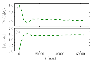
Figure 11: Non-conservation of the (a) inner product [Eq. (67)] and (b) distance between two states [Eq. (27)] by the VGA. The system is the twenty-dimensional coupled Morse potential (51), and state $\psi_{0}$ is the Gaussian wavepacket defined in the text introducing Fig. 6. State $\phi_{0}$ is $\psi_{0}$ displaced by $1\,\textrm{n.u}$ along all its twenty modes.

In Figs. 5, 9, and 10, we showed the geometric properties conserved exactly by the VGA and investigated whether the symplectic integrators can preserve them. Figure 11 displays two properties, the inner product and distance (27), which are not conserved even by the VGA itself. The analytical expression for the inner product of two Gaussians is given in Appendix. B.2. To eliminate numerical errors, we propagated the wavepackets using the eighth-order integrator with a time step of $\Delta t=0.5$ since, as shown in Fig 7, this integrator gives highly accurate results with this time step.

VI Conclusion

In this paper, we have revisited the VGA and analyzed its accuracy, efficiency, and geometric properties. Our results confirm that the VGA is an efficient semiclassical method for simulating weakly anharmonic high-dimensional systems, which are very expensive or beyond reach of exact quantum methods. Furthermore, by comparing the results of the VGA, TGA, and harmonic approximation with exact quantum calculations in several low-dimensional systems, we have confirmed that the VGA, although more computationally expensive, is the most accurate single-trajectory Gaussian-based method. We also verified that the VGA conserves energy and may approximately capture tunneling. The reader should, however, keep in mind that the single Gaussian ansatz is a very restrictive approximation and that, despite conserving the energy and symplectic structure, even a fully converged result of the VGA can be far from the exact quantum solution of a problem.

To reduce the computational cost of the VGA, in Sec. IV, we derived efficient high-order geometric integrators by symmetrically composing the second-order symplectic integrator. These high-order integrators are symplectic, norm-conserving, time-reversible, and for small time steps, energy-conserving. Using the VGA to simulate multi-dimensional coupled Morse potentials, we numerically demonstrated the geometric properties of the symplectic integrators. In particular, we transformed the analytical technique used by Faou and Lubich [19] and by Ohsawa and Leok [21] into a practical numerical method for checking the symplecticity of the geometric integrators.

Although the VGA appears, at first sight, to be an uncontrollable approximation, it is possible to systematically improve VGA using Hagedorn wave packets.[44] The equations of motion of the VGA require expectation values of the potential energy, its gradient, and the Hessian, which are not always analytically available. Although various numerical quadrature techniques exist, they would be too expensive in ab initio real-world applications. One way to reduce this cost is to approximate the potential by its Taylor expansion around the Gaussian’s center. Applying the VGA to the local harmonic approximation of the potential yields the TGA, which conserves neither the symplectic structure nor the effective energy. [67] However, the TGA combined with the ab initio evaluation of the potential has already produced reasonably accurate spectra of a number of polyatomic molecules, such as oligothiophenes, [18, 78] tetrafluorobenzene, ammonia, phosphine, and arsine. [42] By applying the VGA to the local cubic approximation of the potential, one obtains a method that not only improves the accuracy over the TGA, but also preserves both the symplectic structure and the effective energy.  [21, 4, 67] The detailed discussion of this approach, which should still be practical for ab initio calculations of spectra of medium-sized molecules, is deferred to our forthcoming paper. [55]

Supplementary material

See the supplementary material for the convergence and efficiency of the high-order symplectic integrators obtained using the triple-jump and Suzuki-fractal composition schemes, for the analysis of the VGA in Hagedorn’s parametrization [Eq. (12)], and for the separate convergence of individual parameters of the Gaussian wavepacket in both Heller’s [Eq. (4)] and Hagedorn’s parametrizations.

Author declarations

Conflict of interest

The authors have no conflicts to disclose.

Data availability

The data that support the findings of this study are available within the article and its supplementary material.

Appendix A Two non-variational Gaussian wavepacket methods

A.1 Heller’s original thawed Gaussian approximation (TGA)

In the TGA, [11] the potential energy $V$ is replaced by its local harmonic approximation (LHA)

$$V_{\text{LHA}}(q,\psi_{t}) =V(q_{t})+V^{\prime}(q_{t})^{T}\cdot(q-q_{t})$$

$$\quad+(q-q_{t})^{T}\cdot V^{\prime\prime}(q_{t})\cdot(q-q_{t})/2$$ (60)

about the Gaussian’s center $q_{t}$. In Eq. (60), $V(q_{t})$, $V^{\prime}(q_{t})$, and $V^{\prime\prime}(q_{t})$ represent the potential, gradient, and Hessian at $q_{t}$. Replacing $V$ with $V_{\text{LHA}}$ and inserting the thawed Gaussian ansatz (4) [or (12)] into the time-dependent Schrödinger equation (1) gives [11, 78, 68, 67] the equations of motion (6)-(9)[or (13)-(15) in Hagedorn’s parametrization [42]] with coefficients

$$V_{0}=V(q_{t}),\,V_{1}=V^{\prime}(q_{t}),\,V_{2}=V^{\prime\prime}(q_{t}).$$ (61)

A.2 Harmonic approximation

In the harmonic approximation (HA), [79, 67] the potential $V$ is replaced by its second-order Taylor expansion

$$V_{\text{HA}}(q,\psi_{t}) =V(q_{\text{ref}})+V^{\prime}(q_{\text{ref}})^{T}\cdot(q-q_{\text{ref}})$$

$$\quad+(q-q_{\text{ref}})^{T}\cdot V^{\prime\prime}(q_{\text{ref}})\cdot(q-q_{\text{ref}})/2$$ (62)

about a reference geometry $q_{\text{ref}}$. Replacing $V$ with $V_{\text{HA}}$ and inserting the thawed Gaussian ansatz (4) [or (12)] into the time-dependent Schrödinger equation (1), we obtain the equations of motion (6)-(9) [or (13)-(15) in Hagedorn’s parametrization] with coefficients [79, 67]

$$V_{0}=V_{\text{HA}}(q_{t}),\,V_{1}=V_{\text{HA}}^{\prime}(q_{t}),\,V_{2}=V_{\text{HA}}^{\prime\prime}(q_{t}).$$ (63)

Appendix B Various properties of the Gaussian wavepacket

Here, we derive several expressions needed to obtain the equations of motion [Eqs. (6)-(9) with coefficients (10)] and the geometric properties of the VGA.

B.1 Position and momentum covariances

The position and momentum covariance matrices of a Gaussian wavepacket in either Heller’s [Eq. (4)] or Hagedorn’s [Eq. (12)] parametrization are

$$\Sigma_{t} :=\langle(\hat{q}-q_{t})\otimes(\hat{q}-q_{t})^{T}\rangle$$

$$\,\,=(\hbar/2)\,\mathcal{B}_{t}^{-1}=(\hbar/2)\,Q_{t}\cdot Q_{t}^{\dagger},$$ (64)

$$\Pi_{t} :=\langle(\hat{p}-p_{t})\otimes(\hat{p}-p_{t})^{T}\rangle$$

$$\,\,=(\hbar/2)\,A_{t}\cdot\mathcal{B}_{t}^{-1}\cdot A_{t}^{{\dagger}}=(\hbar/2)\,P_{t}\cdot P_{t}^{\dagger}.$$ (65)

The Isserlis theorem [80] implies that the fourth moment of position is [81]

$$\langle x_{j}\,x_{k}\,x_{l}\,x_{m}\rangle=\Sigma_{t,jk}\,\Sigma_{t,lm}+\Sigma_{t,jl}\,\Sigma_{t,km}+\Sigma_{t,jm}\,\Sigma_{t,kl},$$ (66)

where $x:=q-q_{t}$ is a vector of difference coordinates.

B.2 Overlap of Gaussian wavepackets

The overlap of two Gaussian wavepackets is

$$\langle\psi_{1t}| \psi_{2t}\rangle=(\text{det}\,Z)^{-1/2}$$

$$\times\text{exp}\big{\{}(i/\hbar)\big{[}-\delta\lambda^{T}\cdot(\delta W)^{-1}\cdot\delta\lambda/2+\delta\eta\big{]}\big{\}},$$ (67)

where the tensor difference $\delta\Lambda:=\Lambda_{2}-\Lambda^{*}_{1}$ is a shorthand notation used for a particular scalar $\eta$, vector $\lambda$, or matrix $W$, which depend on the Gaussian’s parametrization. For Heller’s parametrization (4), we have [82]

$$Z =(1/2i\pi\hbar)\,\delta W,$$ (68)

$$W =A_{t},$$ (69)

$$\lambda =p_{t}-A_{t}\cdot q_{t},$$ (70)

$$\eta =\gamma_{t}-(\lambda+p_{t})^{T}\cdot q_{t}/2,$$ (71)

whereas for Hagedorn’s parametrization (12), we have

$$Z =\big{(}Q_{1t}^{\dagger}\cdot P_{2t}-P_{1t}^{\dagger}\cdot Q_{2t}\big{)}/(2i),$$ (72)

$$W =P_{t}\cdot Q^{-1}_{t},$$ (73)

$$\lambda =p_{t}-P_{t}\cdot Q^{-1}_{t}\cdot q_{t},$$ (74)

$$\eta =S_{t}-(\lambda+p_{t})^{T}\cdot q_{t}/2.$$ (75)

B.3 Energy of the Gaussian wavepacket

The energy of a normalized Gaussian wavepacket $\psi_{t}$ is computed as the expectation value

$$E_{t}:=\langle\hat{H}\rangle=\langle\hat{T}\rangle+\langle\hat{V}\rangle.$$ (76)

The first term is the kinetic energy

$$\langle\hat{T}\rangle =\langle\hat{p}^{T}\cdot m^{-1}\cdot\hat{p}\rangle/2=\text{Tr}\big{(}m^{-1}\cdot\langle\,\hat{p}\otimes\hat{p}^{T}\rangle\big{)}/2$$

$$=p_{t}^{T}\cdot m^{-1}\cdot p_{t}/2+\text{Tr}\big{(}m^{-1}\cdot\Pi_{t}\big{)}/2,$$ (77)

and the second term is the potential energy

$$\langle\hat{V}\rangle=\int V(q)\,\rho_{t}(q)\,d^{D}q,$$ (78)

where $\rho_{t}$ is the normalized position density

$$\rho_{t}(q):=|\psi_{t}(q)|^{2}=[\text{det}({2\pi\,\Sigma_{t}})]^{-1/2}\,e^{-x^{T}\cdot\Sigma_{t}^{-1}\cdot x/2},$$ (79)

with $x:=q-q_{t}$ and $\Sigma_{t}$ the position covariance (64). Unlike the kinetic energy, the potential energy cannot generally be evaluated analytically.

In the rest of this appendix, we differentiate the energy of the Gaussian wavepacket with respect to its parameters. The derived expressions are used in Appendix C to obtain the equations of motion for the VGA and to demonstrate numerically the preservation of the symplectic structure by the symplectic integrators designed for the VGA.

B.4 Partial derivatives of the kinetic energy

Inserting Eq. (65) for the momentum covariance into Eq. (77) for the kinetic energy gives

$$\langle\hat{T}\rangle =p_{t}^{T}\cdot m^{-1}\cdot p_{t}/2$$

$$+(\hbar/4)\,\text{Tr}\big{(}m^{-1}\cdot\mathcal{A}_{t}\cdot\mathcal{B}_{t}^{-1}\cdot\mathcal{A}_{t}+m^{-1}\cdot\mathcal{B}_{t}\big{)}.$$ (80)

Partial derivatives of $\langle\hat{T}\rangle$ with respect to the parameters $q_{t},\phi_{t}$, and $\gamma_{t}$ vanish. The other derivatives are

$$\partial\langle\hat{T}\rangle/\partial p_{t} =m^{-1}\cdot p_{t},$$ (81)

$$\partial\langle\hat{T}\rangle/\partial\mathcal{A}_{t} =(\hbar/4)\,\big{(}m^{-1}\cdot\mathcal{A}_{t}\cdot\mathcal{B}_{t}^{-1}+\mathcal{B}_{t}^{-1}\cdot\mathcal{A}_{t}\cdot m^{-1}\big{)},$$ (82)

$$\partial\langle\hat{T}\rangle/\partial\mathcal{B}_{t} =(\hbar/4)\,\big{(}m^{-1}-\mathcal{B}_{t}^{-1}\cdot\mathcal{A}_{t}\cdot m^{-1}\cdot\mathcal{A}_{t}\cdot\mathcal{B}_{t}^{-1}\big{)}.$$ (83)

To derive Eqs. (82) and (83), we used the relation

$$\partial\,\text{Tr}[F(X)]/\partial X=f(X)^{T}$$ (84)

for the derivative of the trace of a general function $F(X)$ of a square matrix $X$, and applied it to $X=\mathcal{A}_{t}$ and $\mathcal{B}_{t}$. In Eq. (84), $f(\cdot)$ is the scalar derivative of $F(\cdot)$. [83]

B.5 Partial derivatives of the potential energy

Partial derivatives of the potential energy (78) with respect to the parameters $p_{t},\mathcal{A}_{t},\phi_{t}$, and $\gamma_{t}$ vanish. The other derivatives are

$$\partial\langle\hat{V}\rangle/\partial q_{t} =\langle\hat{V}^{\prime}\rangle,$$ (85)

$$\partial\langle\hat{V}\rangle/\partial\mathcal{B}_{t} =-(\hbar/4)\,\mathcal{B}_{t}^{-1}\cdot\langle\hat{V}^{\prime\prime}\rangle\cdot\mathcal{B}_{t}^{-1}.$$ (86)

To derive Eq. (85), we integrated by parts. Equation (86) follows from Eq. (78) by substituting the derivative

$$\partial\rho_{t}(q)/\partial\mathcal{B}_{t} =\partial\big{[}\text{det}({\mathcal{B}_{t}/\pi\hbar})^{1/2}\,e^{-x^{T}\cdot\mathcal{B}_{t}\cdot x/\hbar}\big{]}/\partial\mathcal{B}_{t}$$

$$=\big{(}\mathcal{B}_{t}^{-1}/2-x\otimes x^{T}/\hbar\big{)}\rho_{t}(q)$$ (87)

of the density (79) and integrating twice by parts. Finally, to derive Eq. (87), we used Eq. (64) for the position covariance and the relation

$$\partial\,\text{det}\mathcal{B}_{t}/\partial\mathcal{B}_{t}=\big{(}\text{det}\mathcal{B}_{t}\big{)}\,(\mathcal{B}_{t}^{-1})^{T}$$ (88)

for the derivative of a determinant. [83]

To find the partial derivatives of the potential energy (78) with respect to Hagedorn’s parameters $Q_{t}$ and $P_{t}$, one needs to express the density (79) in terms of these parameters. To do this, we use Eq. (64) to write

$$\mathcal{B}_{t}^{-1}=Q_{t}\cdot Q_{t}^{\dagger}=\sum_{r=1}^{2}Q_{t}^{(r)}\cdot Q_{t}^{(r)\,T},$$ (89)

where $Q_{t}^{(1)}$ and $Q_{t}^{(2)}$ are the real and imaginary parts of $Q_{t}$. Therefore, the density depends only on $Q_{t}$, implying that $\partial\rho_{t}(q)/\partial P_{t}=0$ and

$$\partial\langle\hat{V}\rangle/\partial\,P_{t}=0.$$ (90)

Furthermore, using Eq. (89) and the chain rule, we have

$$\partial\rho_{t}(q)/\partial Q_{t}^{(r)} =2\,[\partial\rho_{t}(q)/{\partial\mathcal{B}_{t}^{-1}}]\cdot Q_{t}^{(r)}$$

$$=-2\,\mathcal{B}_{t}\cdot[\partial\rho_{t}(q)/{\partial\mathcal{B}_{t}}]\cdot\mathcal{B}_{t}\cdot Q_{t}^{(r)},$$ (91)

which with Eq. (87) gives

$$\partial\langle\hat{V}\rangle/\partial\,Q_{t}^{(r)}=(\hbar/2)\,\langle\hat{V}^{\prime\prime}\rangle\cdot Q_{t}^{(r)},\quad r=1,2.$$ (92)

Similarly, if we differentiate the $n$th potential derivative $\hat{V}^{(n)}$, which is a tensor of rank $n$, we will get a tensor of rank $n+2$ with components

$$\partial\langle\hat{V}^{(n)}\rangle_{k_{1}\dots k_{n}}/\partial Q_{ij}^{(r)}=\frac{\hbar}{2}\,\sum_{l=1}^{D}\,\langle\hat{V}^{(n+2)}\rangle_{k_{1}\dots k_{n}il}\,Q_{lj}^{(r)}.$$ (93)

Appendix C Symplectic wavepacket dynamics

To reveal the symplectic structure of the Schrödinger equation (1), one can identify the complex wavefunction $\Psi_{t}(q)=v_{t}(q)+iw_{t}(q)$ with a real pair $\Psi_{t}=(v_{t},w_{t})$, where $v_{t}:=\text{Re}\,\Psi_{t}$ and $w_{t}:=\text{Im}\,\Psi_{t}$. [84] Since the Hamiltonian $\hat{H}$ is a real operator, Eq. (1) can be written as the canonical Hamiltonian system [84, 19, 50]

$$\hbar\,\dot{\Psi}_{t}=J\,\nabla_{\Psi_{t}}H(\Psi_{t}),$$ (94)

where $H\big{(}\Psi_{t}\big{)}:=\langle\Psi_{t}|\hat{H}|\Psi_{t}\rangle/2$, and

$$J=\begin{pmatrix}0&1\\ -1&0\end{pmatrix}$$ (95)

is the canonical symplectic matrix. From the symplectic point of view, the time-dependent variational principle can be expressed by the real inner product [6]

$$\langle\delta\psi_{t}\,|\hbar\,\dot{\psi}_{t}-J\,\nabla_{\psi_{t}}H(\psi_{t})\rangle=0,$$ (96)

where $\psi_{t}$ is an approximation to the solution of Eq. (94). This is equivalent to requiring that the residual of the Schrödinger equation is always orthogonal to the tangent space $T_{\psi_{t}}M$ of the approximation manifold $M$ at the point $\psi_{t}$. If one maps $\psi_{t}$ to a new coordinate $z_{t}$ with a function $\chi$, i.e., $\psi_{t}=\chi(z_{t})\in M$, Eq. (96) becomes [19, 50]

$$B(z_{t})\,\dot{z}_{t}=\nabla_{z_{t}}H\big{(}\chi(z_{t})\big{)}.$$ (97)

In Eq. (97), $B(z_{t})=\hbar\,X(z_{t})^{T}J^{-1}X(z_{t})$ is the non-canonical symplectic matrix, where $X=(V,W)$ is the real pair of the complex derivative $X_{\mathbb{C}}(z_{t})=\chi^{\prime}(z_{t})=V(z_{t})+iW(z_{t})$. Similar to the canonical symplectic matrix (95), the non-canonical symplectic matrix $B(z_{t})$ is skew-symmetric, but, in general, depends on $z_{t}$. [19, 50]

C.1 Derivations of the VGA equations of motion

In the VGA, the manifold $M$ consists of unnormalized complex Gaussian wavepackets $\chi(z_{t})$ [Eq. (4)] with the squared norm coefficient $I(\mathcal{B}_{t},\delta_{t})$ [Eq. (5)] and parameters

$$z_{t}:=\big{(}q_{t}^{T},p_{t}^{T},\tilde{\mathcal{A}}_{t}^{T},\tilde{\mathcal{B}}_{t}^{T},\phi_{t},\delta_{t}\big{)}^{T}\in\mathbb{R}^{2D+2D^{2}+2},$$ (98)

where $\tilde{\mathcal{A}}_{t}$ and $\tilde{\mathcal{B}}_{t}$ are $D^{2}$-dimensional column vectors containing elements of the real and imaginary parts of the width matrix $A_{t}$ in a column-wise manner, i.e., $\tilde{\mathcal{A}}_{j+D(k-1)}=\mathcal{A}_{jk}$ and $\tilde{\mathcal{B}}_{j+D(k-1)}=\mathcal{B}_{jk}$. The tangent space $T_{\chi}M$ consists of vector derivatives

$$\chi^{\prime}(z_{t})=\bigg{(}\frac{\partial\chi}{\partial q_{t}},\frac{\partial\chi}{\partial p_{t}},\frac{\partial\chi}{\partial\tilde{\mathcal{A}}_{t}},\frac{\partial\chi}{\partial\tilde{\mathcal{B}}_{t}},\frac{\partial\chi}{\partial\phi_{t}},\frac{\partial\chi}{\partial\delta_{t}}\bigg{)},$$ (99)

with

$$\partial\chi/\partial q_{t}=-(i/\hbar)\,(A_{t}\cdot x+p_{t})\,\chi,$$ (100)

$$\partial\chi/\partial p_{t}=(i/\hbar)\,x\,\chi,$$ (101)

$$\partial\chi/\partial\tilde{\mathcal{A}}_{j+D(k-1)}=\partial\chi/\partial\mathcal{A}_{jk}=(i/2\hbar)\,x_{j}\,x_{k}\,\chi,$$ (102)

$$\partial\chi/\partial\tilde{\mathcal{B}}_{j+D(k-1)}=\partial\chi/\partial\mathcal{B}_{jk}=-(1/2\hbar)\,x_{j}\,x_{k}\,\chi,$$ (103)

$$\partial\chi/\partial\phi_{t}=(i/\hbar)\,\chi,$$ (104)

$$\partial\chi/\partial\delta_{t}=-(1/\hbar)\,\chi,$$ (105)

where $x:=q-q_{t}$ is the difference coordinate vector. Using the relation $X^{T}J^{-1}X=-\text{Im}\,X_{\mathbb{C}}^{\dagger}X_{\mathbb{C}}$, [19, 50] we compute the non-canonical symplectic structure matrix of (4) as

$$B(z_{t})=I(\mathcal{B}_{t},\delta_{t})/2$$

$$\times \begin{pmatrix}0&-I_{D}&0&\frac{1}{2}p_{t}\otimes\beta_{t}^{T}&0&\frac{2}{\hbar}p_{t}\\ I_{D}&0&0&0&0&0\\ 0&0&0&-\frac{\hbar}{8}\Gamma_{t}&0&-\frac{1}{2}\beta_{t}\\ -\frac{1}{2}\beta_{t}\otimes p_{t}^{T}&0&\frac{\hbar}{8}\Gamma_{t}&0&\frac{1}{2}\beta_{t}&0\\ 0&0&0&-\frac{1}{2}\beta_{t}^{T}&0&-\frac{2}{\hbar}\\ -\frac{2}{\hbar}p_{t}^{T}&0&\frac{1}{2}\beta_{t}^{T}&0&\frac{2}{\hbar}&0\end{pmatrix},$$ (106)

where $\beta_{t}$ is a $D^{2}$-dimensional vector with components

$$\beta_{j+D(k-1)}:=(2/\hbar)\Sigma_{t,jk}=\big{(}\mathcal{B}^{-1}\big{)}_{jk},$$ (107)

and $\Gamma_{t}$ is a $D^{2}\times D^{2}$ real matrix with components

$$\Gamma_{j+D(k-1),\,l+D(m-1)}=(2/\hbar)^{2}\langle x_{j}\,x_{k}\,x_{l}\,x_{m}\rangle$$

$$\qquad=\big{(}\mathcal{B}^{-1}\big{)}_{jk}\big{(}\mathcal{B}^{-1}\big{)}_{lm}+\big{(}\mathcal{B}^{-1}\big{)}_{jl}\big{(}\mathcal{B}^{-1}\big{)}_{km}$$

$$\qquad\quad+\big{(}\mathcal{B}^{-1}\big{)}_{jm}\big{(}\mathcal{B}^{-1}\big{)}_{kl},$$ (108)

obtained from Eqs. (64) and (66). Using the relations from Appendices B.4 and B.5, the energy gradient with respect to the coordinates $z_{t}$ is

$$\nabla_{z_{t}}H\big{(}\chi(z_{t})\big{)}=I(\mathcal{B}_{t} ,\delta_{t})/2\,\big{(}\langle\hat{V}^{\prime}\rangle,m^{-1}\cdot p_{t},(\hbar/4)\,\epsilon_{t},$$

$$(\hbar/4)\,\zeta_{t},0,-(2/\hbar)\,\langle\hat{H}\rangle\big{)},$$ (109)

where $\langle\hat{H}\rangle$ is defined in Eq. (76) and $\epsilon_{t}$ and $\zeta_{t}$ are $D^{2}$-dimensional vectors with elements

$$\epsilon_{j+D(k-1)} =\big{(}m^{-1}\cdot\mathcal{A}_{t}\cdot\mathcal{B}_{t}^{-1}+\mathcal{B}_{t}^{-1}\cdot\mathcal{A}_{t}\cdot m^{-1}\big{)}_{jk},$$ (110)

$$\zeta_{j+D(k-1)} =\big{(}m^{-1}-\mathcal{B}_{t}^{-1}\cdot\mathcal{A}_{t}\cdot m^{-1}\cdot\mathcal{A}_{t}\cdot\mathcal{B}_{t}^{-1}$$

$$-(2/\hbar) \,\langle\hat{H}\rangle\,\mathcal{B}_{t}^{-1}-\mathcal{B}_{t}^{-1}\cdot\langle\hat{V}^{\prime\prime}\rangle\cdot\mathcal{B}_{t}^{-1}\big{)}_{jk}.$$ (111)

Substituting Eq. (98) for $z_{t}$, Eq. (106) for the symplectic form $B(z_{t})$, and Eq. (109) for the gradient $\nabla_{z_{t}}H\big{(}\chi(z_{t})\big{)}$ into Eq. (97) yields the equations of motion for parameters $q_{t},p_{t},\tilde{\mathcal{A}}_{t},\tilde{\mathcal{B}}_{t},\phi_{t},\text{and}\,\delta_{t}$. Combining the real and imaginary parts of $A_{t}$ and those of $\gamma_{t}$ into single equations, these equations are given by Eqs. (6)-(9) with coefficients (10).

C.2 Symplecticity of the geometric integrators

The geometric integrators designed for the VGA preserve the symplectic structure of the Gaussian wavepackets. [50] To verify this analytically, one should show that the Jacobian $\Phi_{t}^{\prime}=\Phi_{t}^{\prime}(z_{0})$ of the flow $z_{t}=\Phi_{t}(z_{0})$ of an integrator satisfies the relation [50]

$$\Phi_{t}^{\prime}(z_{0})^{T}\cdot B(z_{t})\cdot\Phi_{t}^{\prime}(z_{0})=B(z_{0}).$$ (112)

[Note that matrix $B$ in Eq. (112) is the inverse of matrix $B$ appearing in Eq.(4.2) of Chapter VII of Ref. 50).] The flow of a symplectic integrator is composed of a sequence of kinetic and potential flows, and thus its Jacobian is equal to the matrix product of the Jacobians of the elementary flows. The kinetic flow equations (32) and (33) contain the inverse and determinant of the complex matrix $A_{t}$, and thus it is very difficult to decouple these equations into separate equations for the real and imaginary parts of $A_{t}$ and $\gamma_{t}$. It is much simpler to find the Jacobian of the flow in Hagedorn’s parametrization. Ohsawa found the reduced symplectic structure which corresponds to the Gaussian wavepacket without a phase in the equivalent manifold with phase symmetry. [20] For simplicity, we choose the reduced symplectic form, which is the constant block-diagonal matrix

$$B(z_{t})=\begin{pmatrix}J_{2D}&0&0\\ 0&\frac{\hbar}{2}J_{2D^{2}}&0\\ 0&0&\frac{\hbar}{2}J_{2D^{2}}\end{pmatrix},$$ (113)

with

$$z_{t}:=\bigg{(}q_{t}^{T},p_{t}^{T},\widetilde{,Q_{t}^{(1)}}^{T},\widetilde{P_{t}^{(1)}}^{T},\widetilde{Q_{t}^{(2)}}^{T},\widetilde{P_{t}^{(2)}}^{T}\bigg{)}^{T}\in\mathbb{R}^{2D+4D^{2}},$$ (114)

where $\widetilde{\Lambda}$, which is used for $\Lambda=Q_{t}^{(1)},P_{t}^{(1)},Q_{t}^{(2)}$, and $P_{t}^{(2)}$ is a $D^{2}$-dimensional vector containing elements of the $D\times D$ matrix $\Lambda$ in a column-wise manner, i.e., $\widetilde{\Lambda}_{j+D(k-1)}=\Lambda_{jk}$. Also, $J_{2D}=J\otimes I_{D}$, where $J$ is the two-dimensional symplectic matrix (95), and $J_{2D^{2}}=J_{2D}\otimes I_{D}$. Equations (39)-(42) yield the Jacobian of the kinetic flow $\Phi_{\text{T},t}$, which is the block-diagonal matrix

$$\Phi_{\text{T},t}^{\prime}(z_{0})=\begin{pmatrix}M_{2D}&0&0\\ 0&M_{2D^{2}}&0\\ 0&0&M_{2D^{2}}\end{pmatrix},$$ (115)

where

$$M_{2D}=\begin{pmatrix}I_{D}&t\,m^{-1}\\ 0&I_{D}\end{pmatrix}$$ (116)

is the stability matrix and $M_{2D^{2}}=M_{2D}\otimes I_{D}$. The kinetic flow with Jacobian (115) is symplectic, i.e., $\Phi_{\text{T},t}^{\prime}(z_{0})^{T}\cdot B(z_{t})\cdot\Phi_{\text{T},t}^{\prime}(z_{0})=B(z_{0}),$ because

$$M_{2D}^{T}\cdot J_{2D}\cdot M_{2D}=\begin{pmatrix}I_{D}&0\\ t\,m^{-1}&I_{D}\end{pmatrix}\begin{pmatrix}0&-I_{D}\\ I_{D}&t\,m^{-1}\end{pmatrix}=J_{2D},$$ (117)

and using matrix and tensor multiplication

$$M_{2D^{2}}^{T} \cdot J_{2D^{2}}\cdot M_{2D^{2}}$$

$$=\big{(}M_{2D}^{T}\otimes I_{D}\big{)}\cdot\big{(}J_{2D}\otimes I_{D}\big{)}\cdot\big{(}M_{2D}\otimes I_{D}\big{)}$$

$$=\big{(}M_{2D}^{T}\cdot J_{2D}\cdot M_{2D}\big{)}\otimes I_{D}=J_{2D^{2}}.$$ (118)

Similarly, Eqs. (44)-(47) imply that the Jacobian of the potential flow $\Phi_{\text{V},t}$ is the $(2D+4D^{2})$-dimensional matrix

$$\Phi_{\text{V},t}^{\prime}(z_{0})=I_{2D+4D^{2}}-t\begin{pmatrix}0&0&0&0&0&0\\ a&0&b^{(1)}&0&b^{(2)}&0\\ 0&0&0&0&0&0\\ c^{(1)}&0&d^{(11)}&0&d^{(12)}&0\\ 0&0&0&0&0&0\\ c^{(2)}&0&d^{(21)}&0&d^{(22)}&0\end{pmatrix},$$ (119)

where

$$a_{j,k} =\langle\hat{V}^{\prime\prime}\rangle_{jk},$$ (120)

$$b_{j,D(k-1)+l}^{(r)} =(\hbar/2)\,\langle\hat{V}^{\prime\prime\prime}\rangle_{jkm}\,Q_{t,ml}^{(r)},$$ (121)

$$c_{D(j-1)+k,l}^{(r)} =\langle\hat{V}^{\prime\prime\prime}\rangle_{jml}\,Q_{t,mk}^{(r)},$$ (122)

$$d_{D(j-1)+k,\,D(l-1)+m}^{(rs)} =(\hbar/2)\,\langle\hat{V}^{(4)}\rangle_{jnlp}\,Q_{t,nk}^{(r)}\,Q_{t,pm}^{(s)}$$

$$\quad+\langle\hat{V}^{\prime\prime}\rangle_{jn}\,\delta_{nl}\,\delta_{km}\,\delta_{rs}$$ (123)

specify the components of the $D\times D$ matrix $a$, $D\times D^{2}$ matrix $b^{(r)}$, $D^{2}\times D$ matrix $c^{(r)}$, and $D^{2}\times D^{2}$ matrix $d^{(rs)}$ for all $r,s\in\{1,2\}$. In Eqs. (121)-(123), $\hat{V}^{\prime\prime\prime}:=V^{\prime\prime\prime}(q)|_{q=\hat{q}}$ and $\hat{V}^{(4)}:=V^{(4)}(q)|_{q=\hat{q}}$. It is easy to show that the potential flow with Jacobian (119) is symplectic, i.e., $\Phi_{\text{V},t}^{\prime}(z_{0})^{T}\cdot B(z_{t})\cdot\Phi_{\text{V},t}^{\prime}(z_{0})=B(z_{0})$, if and only if

$$a^{T} =a,$$ (124)

$$\big{(}b^{(r)}\big{)}^{T} =(\hbar/2)\,c^{(r)},$$ (125)

$$\big{(}d^{(rs)}\big{)}^{T} =d^{(sr)}.$$ (126)

Because $\langle\hat{V}^{\prime\prime}\rangle$, $\langle\hat{V}^{\prime\prime\prime}\rangle$, and $\langle\hat{V}^{(4)}\rangle$ are totally symmetric, Eqs. (120)-(123) for $a$, $b^{(r)}$, $c^{(r)}$ and $d^{(rs)}$ imply that conditions (124)-(126) hold for the Jacobian (119), and thus the potential flow is symplectic. Since both kinetic and potential flows are symplectic, any composition of them is also symplectic. This proves the conservation of the symplectic structure by the geometric integrators. In Sec.V.2, we verified their symplecticity numerically by measuring the accuracy with which Eq. (112) is satisfied if $\Phi_{t}(z_{0})$ denotes the composed flow consisting many steps, each of which, in turn, is composed by several potential and kinetic substeps. For that, the Jacobian $\Phi^{\prime}_{t}(z_{0})$ of the composed flow appearing in Eq. (112) was obtained by matrix multiplication of the Jacobians (115) and (119) of all kinetic and potential steps.

Appendix D Expectation values in a Gaussian wavepacket

In this appendix, we derive the expectation values in a Gaussian wavepacket of the potential energy, gradient, and Hessian of the multi-dimensional quartic and coupled Morse potentials.

D.1 Quartic potential and its derivatives

An important class of potentials consists of the quartic polynomials, which have applications in many areas of research, including molecular force-field design [85, 86] and tunneling theory. [87, 88] We consider the most general form of a $D$-dimensional quartic potential

$$V(q) =V(q_{\text{ref}})+V^{\prime}(q_{\text{ref}})^{T}\cdot x+x^{T}\cdot V^{\prime\prime}(q_{\text{ref}})\cdot x/2$$

$$\quad+V^{\prime\prime\prime}(q_{\text{ref}})_{ijk}\,x_{i}\,x_{j}\,x_{k}/3!$$

$$\quad+V^{(4)}(q_{\text{ref}})_{ijkl}\,x_{i}\,x_{j}\,x_{k}\,x_{l}/4!,$$ (127)

where the scalar $V(q_{\text{ref}})$, vector $V^{\prime}(q_{\text{ref}})$, matrix $V^{\prime\prime}(q_{\text{ref}})$, rank-$3$ tensor $V^{\prime\prime\prime}(q_{\text{ref}})$, and rank-$4$ tensor $V^{(4)}(q_{\text{ref}})$ are the potential energy and its first four derivatives at a reference position $q_{\text{ref}}$. Here, $x:=q-q_{\text{ref}}$ is a $D$-dimensional vector with elements $x_{i}$. The gradient and Hessian of the quartic potential are

$$V^{\prime}(q)_{i} =V^{\prime}(q_{\text{ref}})_{i}+V^{\prime\prime}(q_{\text{ref}})_{ij}\,x_{j}$$

$$\quad+V^{\prime\prime\prime}(q_{\text{ref}})_{ijk}\,x_{j}\,x_{k}/2$$

$$\quad+V^{(4)}(q_{\text{ref}})_{ijkl}\,x_{j}\,x_{k}\,x_{l}/3!,$$ (128)

$$V^{\prime\prime}(q)_{ij} =V^{\prime\prime}(q_{\text{ref}})_{ij}+V^{\prime\prime\prime}(q_{\text{ref}})_{ijk}\,x_{k}$$

$$\quad+V^{(4)}(q_{\text{ref}})_{ijkl}\,x_{k}\,x_{l}/2.$$ (129)

Using Eqs. (64) and (66) and the fact that $V^{\prime\prime}(q_{\text{eq}})$, $V^{\prime\prime\prime}(q_{\text{eq}})$, and $V^{(4)}(q_{\text{eq}})$ are totally symmetric tensors, the expectation values of the quartic potential and its first two derivatives in a Gaussian wavepacket are

$$\langle\hat{V}\rangle =V(q_{\text{ref}})+\text{Tr}[V^{\prime\prime}(q_{\text{ref}})\cdot\Sigma_{t}]/2$$

$$\quad+V^{(4)}(q_{\text{ref}})_{ijkl}\,\Sigma_{t,ij}\,\Sigma_{t,kl}/8,$$ (130)

$$\langle\hat{V}^{\prime}\rangle_{i} =V^{\prime}(q_{\text{ref}})_{i}+V^{\prime\prime\prime}(q_{\text{ref}})_{ijk}\,\Sigma_{t,jk}/2,$$ (131)

$$\langle\hat{V}^{\prime\prime}\rangle_{ij} =V^{\prime\prime}(q_{\text{ref}})_{ij}+V^{(4)}(q_{\text{ref}})_{ijkl}\,\Sigma_{t,kl}/2.$$ (132)

D.2 Coupled Morse potential and its derivatives

The coupled Morse potential (51) is introduced in the main text. The expectation values of this potential and its first four derivatives are

$$\langle\hat{V}\rangle =V_{\text{eq}}+\sum_{j=1}^{D}\langle V_{j}(\hat{q}_{j})\rangle+\langle V_{\text{cpl}}(\hat{q})\rangle,$$ (133)

$$\langle\hat{V}^{(k)}\rangle =\sum_{j=1}^{D}\langle V_{j}^{(k)}(\hat{q}_{j})\rangle+\langle V_{\text{cpl}}^{(k)}(\hat{q})\rangle,$$ (134)

where $k\in\{1,2,3,4\}$,

$$V_{j}^{(k)}(q_{j})=(-1)^{k-1}2\,d_{e}^{\prime}\big{(}a_{j}^{\prime}\big{)}^{k}\,\big{[}y(a_{j}^{\prime},q_{j})-2^{k-1}y(a_{j}^{\prime},q_{j})^{2}\big{]}$$ (135)

is the $k$th derivative of the one-dimensional Morse potential (52), and

$$V_{\text{cpl}}^{(k)}(q)_{l_{1}\dots l_{k}} =(-1)^{k-1}\,2\,d_{e}\,a_{l_{1}}\dots a_{l_{k}}\,$$

$$\qquad\big{[}y(a,q)-2^{k-1}\,y(a,q)^{2}\big{]}$$ (136)

is the $k$th derivatives of the $D$-dimensional coupling term (54).

Expectation value of the Morse variable (55) in the Gaussian wavepacket can be evaluated analytically as

$$\langle y(a,q)\rangle =\int e^{-a^{T}\cdot(q-q_{\text{eq}})}\,\rho_{t}(q)\,d^{D}q$$

$$=\big{[}\text{det}\big{(}{2\pi\,\Sigma_{t}^{-1}}\big{)}\big{]}^{-1/2}\,e^{-a^{T}\cdot(q_{t}-q_{\text{eq}})}$$

$$\quad\times\int e^{-(q-q_{t})^{T}\cdot\Sigma_{t}^{-1}\cdot(q-q_{t})/2-a^{T}\cdot(q-q_{\text{t}})}\,d^{D}q$$

$$=e^{-a^{T}\cdot(q_{t}-q_{\text{eq}})+a^{T}\cdot\Sigma_{t}\cdot a/2}$$

$$=y(a,q_{t})\,z(a),$$ (137)

where we defined the “Morse Gaussian variable”

$$z(a):=\exp\big{(}a^{T}\cdot\Sigma_{t}\cdot a/2\big{)}.$$ (138)

Likewise,

$$\langle y(a,q)^{2}\rangle=y(a,q_{t})^{2}\,z(a)^{4}.$$ (139)

To find the expectation value of a one-dimensional Morse variable $y_{j}(a_{j}^{\prime},q_{j})$ in a multi-dimensional Gaussian wavepacket, we considered an auxiliary vector $\tilde{a}$ with $D$ components $\tilde{a}_{k}=a_{j}^{\prime}\,\delta_{jk}$. Noting that

$$y_{j}(a_{j}^{\prime},q_{j})=e^{-a_{j}^{\prime}\,(q_{j}-q_{\text{eq},j})}=e^{-\tilde{a}\cdot(q-q_{\text{eq}})}=y(\tilde{a},q),$$ (140)

defining a one-dimensional Morse Gaussian variable

$$z_{j}(a_{j}^{\prime}):=e^{\Sigma_{t,jj}\,{a_{j}^{\prime}}^{2}/2}=e^{\tilde{a}^{T}\cdot\Sigma_{t}\cdot\tilde{a}/2}=z(\tilde{a}),$$ (141)

and using the results (137) and (139), we find that

$$\langle y_{j}(a_{j}^{\prime},q_{j})\rangle =\langle y(\tilde{a},q)\rangle=y(\tilde{a},q_{t})\,z(\tilde{a})$$

$$=y_{j}(a_{j}^{\prime},q_{t,j})\,z_{j}(a_{j}^{\prime}),$$ (142)

$$\langle y_{j}(a_{j}^{\prime},q_{j})^{2}\rangle =\langle y(\tilde{a},q)^{2}\rangle=y(\tilde{a},q_{t})^{2}\,z(\tilde{a})^{4}$$

$$=y_{j}(a_{j}^{\prime},q_{t,j})^{2}\,z_{j}(a_{j}^{\prime})^{4}.$$ (143)

From Eqs. (142) and (143), we obtain expectation values of the one-dimensional Morse potential (52) and its derivative (135):

$$\langle V_{j}(\hat{q}_{j})\rangle =d_{e}^{\prime}\,(1-2\,m_{j}+n_{j}),$$ (144)

$$\langle V_{j}^{(k)}(\hat{q}_{j})\rangle =(-1)^{k-1}2\,d_{e}^{\prime}\,\big{(}a_{j}^{\prime}\big{)}^{k}\,(m_{j}-2^{k-1}\,\,n_{j}),$$ (145)

where we introduced $m_{j}:=y_{j}(a_{j}^{\prime},q_{t,j})\,z_{j}(a_{j}^{\prime})$ and $n_{j}:=y_{j}(a_{j}^{\prime},q_{t,j})^{2}\,z_{j}(a_{j}^{\prime})^{4}$ to simplify the notation. Similarly, Eqs.(137) and (139) give expectation values of the coupling term (54) and its derivative (136):

$$\langle V_{\text{cpl}}(\hat{q})\rangle =d_{e}\,(1-2\,M+N),$$ (146)

$$\langle V_{\text{cpl}}^{(k)}(\hat{q})\rangle_{l_{1}\dots l_{k}} =(-1)^{k-1}\,2\,d_{e}\,a_{l_{1}}\dots a_{l_{k}}\,(M-2^{k-1}N),$$ (147)

where $M:=y(a,q_{t})\,z(a)$ and $N:=y(a,q_{t})^{2}\,z(a)^{4}$.

References

- Nitzan [2006] A. Nitzan, Chemical dynamics in condensed phases: relaxation, transfer and reactions in condensed molecular systems (Oxford university press, 2006).
- Tannor [2007] D. J. Tannor, Introduction to Quantum Mechanics: A Time-Dependent Perspective (University Science Books, Sausalito, 2007).
- Heller [2018] E. J. Heller, The semiclassical way to dynamics and spectroscopy (Princeton University Press, Princeton, NJ, 2018).
- Pattanayak and Schieve [1994] A. K. Pattanayak and W. C. Schieve, Phys. Rev. E 50, 3601 (1994).
- Pattanayak and Schieve [1997] A. K. Pattanayak and W. C. Schieve, Phys. Rev. E 56, 278 (1997).
- Lubich [2008] C. Lubich, From Quantum to Classical Molecular Dynamics: Reduced Models and Numerical Analysis, 12th ed. (European Mathematical Society, Zürich, 2008).
- Faou, Gradinaru, and Lubich [2009] E. Faou, V. Gradinaru, and C. Lubich, SIAM J. Sci. Comp. 31, 3027 (2009).
- Richings et al. [2015] G. W. Richings, I. Polyak, K. E. Spinlove, G. A. Worth, I. Burghardt, and B. Lasorne, Int. Rev. Phys. Chem. 34, 269 (2015).
- Garashchuk [2021] S. Garashchuk, in Basis Sets in Computational Chemistry (Springer, 2021) pp. 215–252.
- Edery [2021] A. Edery, Phys. Rev. D 104, 125015 (2021).
- Heller [1975] E. J. Heller, J. Chem. Phys. 62, 1544 (1975).
- Heller [1976a] E. J. Heller, J. Chem. Phys. 65, 4979 (1976a).
- Heller [1981a] E. J. Heller, J. Chem. Phys. 75, 2923 (1981a).
- Hagedorn [1980] G. A. Hagedorn, Commun. Math. Phys. 71, 77 (1980).
- Hagedorn [1998] G. A. Hagedorn, Ann. Phys. (NY) 269, 77 (1998).
- Lasorne et al. [2006] B. Lasorne, M. J. Bearpark, M. A. Robb, and G. A. Worth, Chem. Phys. Lett. 432, 604 (2006).
- Ben-Nun and Martínez [1998] M. Ben-Nun and T. J. Martínez, Chem. Phys. Lett. 298, 57 (1998).
- Wehrle, Šulc, and Vaníček [2014] M. Wehrle, M. Šulc, and J. J. L. Vaníček, J. Chem. Phys. 140, 244114 (2014).
- Faou and Lubich [2006] E. Faou and C. Lubich, Comput. Visual. Sci. 9, 45 (2006).
- Ohsawa [2015] T. Ohsawa, Lett. Math. Phys. 105, 1301 (2015).
- Ohsawa and Leok [2013] T. Ohsawa and M. Leok, J. Phys. A 46, 405201 (2013).
- Martínez, Ben-Nun, and Levine [1996] T. J. Martínez, M. Ben-Nun, and R. D. Levine, J. Phys. C 100, 7884 (1996).
- Ben-Nun, Quenneville, and Martínez [2000] M. Ben-Nun, J. Quenneville, and T. J. Martínez, J. Phys. Chem. A 104, 5161 (2000).
- Curchod and Martínez [2018] B. F. E. Curchod and T. J. Martínez, Chem. Rev. 118, 3305 (2018).
- Shalashilin and Child [2004] D. V. Shalashilin and M. S. Child, J. Chem. Phys. 121, 3563 (2004).
- Sawada et al. [1985] S. Sawada, R. Heather, B. Jackson, and H. Metiu, J. Chem. Phys. 83, 3009 (1985).
- Sawada and Metiu [1986a] S. Sawada and H. Metiu, J. Chem. Phys. 84, 6293 (1986a).
- Sawada and Metiu [1986b] S. Sawada and H. Metiu, J. Chem. Phys. 84, 227 (1986b).
- Worth and Burghardt [2003] G. A. Worth and I. Burghardt, Chem. Phys. Lett. 368, 502 (2003).
- Shalashilin [2009] D. V. Shalashilin, J. Chem. Phys. 130, 244101 (2009).
- Shalashilin [2010] D. V. Shalashilin, J. Chem. Phys. 132, 244111 (2010).
- Šulc et al. [2013] M. Šulc, H. Hernández, T. J. Martínez, and J. J. L. Vaníček, J. Chem. Phys. 139, 034112 (2013).
- Miller [2001] W. H. Miller, J. Phys. Chem. A 105, 2942 (2001).
- Herman and Kluk [1984] M. F. Herman and E. Kluk, Chem. Phys. 91, 27 (1984).
- Grossmann [2006] F. Grossmann, J. Chem. Phys. 125, 014111 (2006).
- Ceotto et al. [2009] M. Ceotto, S. Atahan, G. F. Tantardini, and A. Aspuru-Guzik, J. Chem. Phys. 130, 234113 (2009).
- Ceotto, Di Liberto, and Conte [2017] M. Ceotto, G. Di Liberto, and R. Conte, Phys. Rev. Lett. 119, 010401 (2017).
- Gabas, Di Liberto, and Ceotto [2019] F. Gabas, G. Di Liberto, and M. Ceotto, J. Chem. Phys. 150, 224107 (2019).
- Lee and Heller [1982] S. Y. Lee and E. J. Heller, J. Chem. Phys. 76, 3035 (1982).
- Wehrle, Oberli, and Vaníček [2015] M. Wehrle, S. Oberli, and J. J. L. Vaníček, J. Phys. Chem. A 119, 5685 (2015).
- Patoz, Begušić, and Vaníček [2018] A. Patoz, T. Begušić, and J. J. L. Vaníček, J. Phys. Chem. Lett. 9, 2367 (2018).
- Begušić, Tapavicza, and Vaníček [2022] T. Begušić, E. Tapavicza, and J. J. L. Vaníček, J. Chem. Theory Comput. 18, 3065 (2022).
- Coalson and Karplus [1990] R. D. Coalson and M. Karplus, J. Chem. Phys. 93, 3919 (1990).
- Lasser and Lubich [2020] C. Lasser and C. Lubich, Acta Numerica 29, 229 (2020).
- Dirac [1930] P. A. M. Dirac, Math. Proc. Camb. Phil. Soc. 26, 376 (1930).
- Frenkel [1934] J. Frenkel, Wave mechanics (Clarendon Press, Oxford, 1934).
- McLachlan [1964] A. McLachlan, Mol. Phys. 8, 39 (1964).
- Heller [1976b] E. J. Heller, J. Chem. Phys. 64, 63 (1976b).
- Kramer and Saraceno [1980] P. Kramer and M. Saraceno, Geometry of the time-dependent variational principle in quantum mechanics (Springer Berlin Heidelberg, Berlin, Heidelberg, 1980).
- Hairer, Lubich, and Wanner [2006] E. Hairer, C. Lubich, and G. Wanner, Geometric Numerical Integration: Structure-Preserving Algorithms for Ordinary Differential Equations (Springer Berlin Heidelberg New York, 2006).
- Buch [2002] V. Buch, J. Chem. Phys. 117, 4738 (2002).
- Hasegawa [2014] H. Hasegawa, Phys. Lett. A 378, 691 (2014).
- Heather and Metiu [1985] R. Heather and H. Metiu, Chem. Phys. Lett. 118, 558 (1985).
- Poirier [2017] B. Poirier, “Dirac–Frenkel Variational Principle as Applied to Quantum Trajectories,” (2017).
- Moghaddasi Fereidani and Vaníček [2023] R. Moghaddasi Fereidani and J. J. L. Vaníček, “High-order geometric integrators for the local cubic variational thawed gaussian wavepacket dynamics,” (2023).
- Leimkuhler and Reich [2004] B. Leimkuhler and S. Reich, Simulating Hamiltonian Dynamics (Cambridge University Press, 2004).
- Yoshida [1990] H. Yoshida, Phys. Lett. A 150, 262 (1990).
- Suzuki [1990] M. Suzuki, Phys. Lett. A 146, 319 (1990).
- McLachlan [1995] R. I. McLachlan, SIAM J. Sci. Comp. 16, 151 (1995).
- Wehrle, Šulc, and Vaníček [2011] M. Wehrle, M. Šulc, and J. J. L. Vaníček, Chimia 65, 334 (2011).
- Sofroniou and Spaletta [2005] M. Sofroniou and G. Spaletta, Optim. Method Softw. 20, 597 (2005).
- Choi and Vaníček [2019] S. Choi and J. J. L. Vaníček, J. Chem. Phys. 150, 204112 (2019).
- Roulet, Choi, and Vaníček [2019] J. Roulet, S. Choi, and J. J. L. Vaníček, J. Chem. Phys. 150, 204113 (2019).
- Born and Oppenheimer [1927] M. Born and R. Oppenheimer, Ann. d. Phys. 389, 457 (1927).
- Heller [1981b] E. J. Heller, Acc. Chem. Res. 14, 368 (1981b).
- Roulet and Vaníček [2021] J. Roulet and J. J. L. Vaníček, J. Chem. Phys. 154, 154106 (2021).
- Vaníček [2023] J. J. L. Vaníček, (2023), 10.48550/ARXIV.2302.10221.
- Vaníček and Begušić [2021] J. J. L. Vaníček and T. Begušić, in Molecular Spectroscopy and Quantum Dynamics, edited by R. Marquardt and M. Quack (Elsevier, 2021) pp. 199–229.
- Kramer and Saraceno [1981] P. Kramer and M. Saraceno, Geometry of the time-dependent variational principle in quantum mechanics, Lecture notes in physics, Vol. 140 (Springer-Verlag, Berlin, 1981).
- Beck et al. [2000] M. Beck, A. Jäckle, G. Worth, and H.-D. Meyer, Phys. Rep. 324, 1 (2000).
- Habershon [2012] S. Habershon, J. Chem. Phys. 136, 014109 (2012).
- Joubert-Doriol and Izmaylov [2015] L. Joubert-Doriol and A. F. Izmaylov, J. Chem. Phys. 142, 134107 (2015).
- Hackl et al. [2020] L. Hackl, T. Guaita, T. Shi, J. Haegeman, E. Demler, and J. I. Cirac, SciPost Phys. 9, 048 (2020).
- Kahan and Li [1997] W. Kahan and R.-C. Li, Math. Comput. 66, 1089 (1997).
- Choi and Vaníček [2021] S. Choi and J. J. L. Vaníček, J. Chem. Phys. 155, 124104 (2021).
- Thorwart, Grifoni, and Hänggi [2001] M. Thorwart, M. Grifoni, and P. Hänggi, Adv. Phys. 293, 15 (2001).
- Razavy [2003] M. Razavy, Quantum Theory of Tunneling (World Scientific Publishing, Singapore, 2003).
- Begušić, Cordova, and Vaníček [2019] T. Begušić, M. Cordova, and J. J. L. Vaníček, J. Chem. Phys. 150, 154117 (2019).
- Tannor and Heller [1982] D. J. Tannor and E. J. Heller, J. Chem. Phys. 77, 202 (1982).
- Isserlis [1918] L. Isserlis, Biometrika 12, 134 (1918).
- Brookes [2011] M. Brookes, “The Matrix Reference Manual,” [online] http://www.ee.imperial.ac.uk/hp/staff/dmb/matrix/intro.html (2011).
- Begušić and Vaníček [2020] T. Begušić and J. J. L. Vaníček, J. Chem. Phys. 153, 184110 (2020).
- Petersen and Pedersen [2012] K. B. Petersen and M. S. Pedersen, “The matrix cookbook,” (2012).
- Marsden and Ratiu [1999] J. E. Marsden and T. S. Ratiu, Introduction to mechanics and symmetry: a basic exposition of classical mechanical systems, Vol. 17 (Springer Science & Business Media, 1999).
- Vande Linde and Hase [1990] S. R. Vande Linde and W. L. Hase, J. Phys. Chem. 94, 2778 (1990).
- Yagi et al. [2004] K. Yagi, K. Hirao, T. Taketsugu, M. W. Schmidt, and M. S. Gordon, J. Chem. Phys. 121, 1383 (2004).
- Mandelli, Aieta, and Ceotto [2022] G. Mandelli, C. Aieta, and M. Ceotto, J. Chem. Theory Comput. 18, 623 (2022).
- Masoumi, Olum, and Wachter [2017] A. Masoumi, K. D. Olum, and J. M. Wachter, J. Cosmol. Astropart. Phys. 2017, 022 (2017).