Next-to-leading power corrections to the event shape variables

Abstract

We investigate the origin of next-to-leading power corrections to the event shapes thrust and $c$-parameter, at next-to-leading order. For both event shapes we trace the origin of such terms in the exact calculation, and compare with a recent approach involving the eikonal approximation and momentum shifts that follow from the Low-Burnett-Kroll-Del Duca theorem. We assess the differences both analytically and numerically. For the $c$-parameter both exact and approximate results are expressed in terms of elliptic integrals, but near the elastic limit it exhibits patterns similar to the thrust results.

I Introduction

Providing precise estimates for cross-sections in perturbative QCD is needed to match the ever increasing precision of collider physics measurements. Two complementary directions are pursued in this endeavour. In one, exact higher order calculations in the coupling $\alpha_{s}$ are performed, and methods thereto developed. In the other, all-order results are derived in certain kinematic limits, where associated classes of logarithmic terms are enhanced; the latter can often be resummed to all orders, using a varied and ever expanding set of methods. A highly relevant region in this regard is the near-elastic region (which we loosely refer to here also as the threshold region), where the phase space for emitted particles is limited. In such a situation, the cancellation of infrared singularities, guaranteed by the KLN theorem [1, 2], is incomplete in the sense that it leaves large logarithmic remainders at any order in perturbation theory. Our analysis in this paper is relevant for the second direction.

To be more specific, if $\xi$ is a dimensionless kinematic variable, such that $\xi\rightarrow 0$ towards the elastic region, the corresponding differential cross-section has the generic form

$$\frac{d\sigma}{d\xi}\,=\,\sum_{n=0}^{\infty}\left(\frac{\alpha_{s}}{\pi}\right)^{n}\,\left[\sum_{m=0}^{2n-1}c_{nm}^{\text{LP}}\left(\frac{\log^{m}\xi}{\xi}\right)_{+}+\,c_{n}^{(\delta)}\delta(\xi)+\,\sum_{m=0}^{2n-1}c_{nm}^{\text{NLP}}\,\log^{m}\xi\,+\,\ldots\right]\,.$$ (1)

The first term on the right in the above equation is well-known to originate from soft and/or collinear radiation and, together with the second term, makes up the leading power (LP) terms. Much is known about LP terms to arbitrary order, and there have been numerous approaches towards their resummation [3, 4, 5, 6, 7, 8, 9, 10, 11, 12, 13, 14, 15, 16, 17, 18] and power correction studies [19, 20]. Reviews on some of these different approaches can be found in [21, 22, 23, 24, 25].

The last term on the right represents next-to-leading power (NLP) terms. These originate from both soft gluon and soft quark emissions. Although suppressed by a power of $\xi$, they can be relevant, since they grow logarithmically towards threshold. In contrast to the LP terms, the precise organization of these NLP terms to all orders and arbitrary logarithmic accuracy are not yet clear. In this paper we focus on such NLP terms for two event shapes in $e^{+}e^{-}$ collisions: thrust and the $C$-parameter. These observables are interesting in this regard because, in contrast to most earlier studies, all QCD effects reside in the final state, and because their definition involves special phase space constraints that were not considered so far [26, 27, 28, 29]. For these observables our aim is to trace the origin of the NLP terms near the elastic limit, to examine to what extent there is a common pattern of NLP terms, and assess their size.

Patterns among NLP terms have been studied for various processes [30, 31, 32, 33, 34, 35, 36, 37, 38, 39, 40, 41, 42]. For a number of observables their numerical contribution can be significant [43, 44, 45, 46, 47, 48]. The all-order resummation of NLP terms has been pursued through different approaches, such as a diagrammatic and a path integral approach given in [49, 50], while a physical kernel approach is pursued in [51, 52, 53]. From direct QCD formalism, the development of factorization theorems for NLP terms extending from LP terms are studied in [30, 31, 54, 55, 56, 57, 58] (for NLP factorization see, [59]). The study of NLP effects in the framework of SCET has many aspects, and the active studies are done in the operators contributing at NLP level [60, 61, 62, 63, 64, 65, 66, 67], the development of factorization [34, 33, 42, 68], and the explicit studies of physical observables [69, 70, 71, 32, 72, 73, 36, 74, 75, 76, 77, 39].

Event shapes, which probe final state dynamics through geometrical constraints, have long been used to develop QCD ideas [78, 79, 80, 81], e.g. the development of resummation and fixed-order computations [82, 83, 78, 84, 85, 86, 87]. They have also played a vital role in extracting the strong coupling constant [88, 89, 90, 91]. Here we examine to what extent NLP terms for two event shapes can be predicted using the kinematical shift method [92, 46], as well as the soft quark emission approximation.

Our paper is organized as follows. We compute the thrust distribution in shifted approximation in section III to assess the relevance of NLP terms. We perform a similar assessment in section IV, which is considerably more complicated. We conclude in section V, while appendices contain certain technical aspects of elliptic functions, and a summary table of our results.

II Next-to-leading power terms and kinematical shifts

It was recently shown [92] that NLP terms, at next-to-leading order (NLO) and to the extent that they are due to soft gluon radiation, may be derived efficiently using a combination of the eikonal approximation and kinematical shifts, in first instance for colour singlet final states. The method holds for matrix elements and thus for differential distributions, and was subsequently extended to final state radiation in [46]. It rests in essence on the Low-Burnett-Kroll-Del Duca (LBKD) theorem [93, 94, 95], which enables the expression of the one-gluon emission amplitude in terms of the elastic amplitude (even if the latter contains loops, such as in the case of Higgs, or multi-Higgs production). The NLO matrix element up to NLP accuracy can be written as a combination of scalar, spin, and orbital terms:

$$\mathcal{M}_{\text{NLP}}\,=\,\mathcal{M}_{\text{scal}}+\mathcal{M}_{\text{spin}}+\mathcal{M}_{\text{orb}}\,.$$ (2)

The scalar term is essentially a multiplicative term containing the LP eikonal approximation. The spin-dependent term is of NLP accuracy, as the eikonal approximation cannot resolve emitter spin. The orbital term, also of NLP accuracy, involves derivative operators. These can be represented as a first-order Taylor expansion of kinematically shifted momenta. Combining these terms for the production of colour singlet particles yields the expression

$$\overline{\sum}|\mathcal{M}_{\text{shift}}|^{2}\,=\, g_{s}^{2}N_{c}(N_{c}^{2}-1)\frac{2p_{1}\cdot p_{2}}{(p_{1}\cdot p_{3})(p_{2}\cdot p_{3})}$$

$$\times|\mathcal{M}_{0}(p_{1}-\delta p_{1},p_{2}-\delta p_{2})|^{2},$$ (3)

where $|\mathcal{M}_{0}(p_{1},p_{2})|^{2}$ is the matrix element squared at the leading order (LO), and $\overline{\sum}$ denotes the sum (average) over the final (initial) state spins and colours, $p_{3}$ is the momentum of the emitted radiation, and $p_{1}$, $p_{2}$ are the momenta of the particles already present at the born level. The shifts in the momenta are given by

$$\delta p_{1}^{\mu} \,\,=\,-\frac{1}{2}\left(\frac{p_{2}\cdot p_{3}}{p_{1}\cdot p_{2}}p_{1}^{\mu}-\frac{p_{1}\cdot p_{3}}{p_{1}\cdot p_{2}}p_{2}^{\mu}+p_{3}^{\mu}\right),$$

$$\delta p_{2}^{\mu} \,\,=\,-\frac{1}{2}\left(\frac{p_{1}\cdot p_{3}}{p_{1}\cdot p_{2}}p_{2}^{\mu}-\frac{p_{2}\cdot p_{3}}{p_{1}\cdot p_{2}}p_{1}^{\mu}+p_{3}^{\mu}\right).$$ (4)

Expressions (3) and (4) yield the dominant NLP contributions to the NLO matrix element. We now turn to examine the implications of this for the two event shapes.

III Thrust

Thrust [96] in $e^{+}e^{-}$ collisions is defined as

$$T\,=\,\underset{\bf{\hat{n}}}{\rm{max}}\ \frac{\sum_{i}|{\bf{p}_{i}}\cdot{\bf{\hat{n}}}|}{\sum_{i}E_{i}}\,,$$ (5)

where $\bf{p}_{i}$ and $E_{i}$ are the three-momentum and energy of the $i^{\text{th}}$ particle present in the final state. The unit vector $\bf{\hat{n}}$ that maximizes the sum in the numerator is the thrust axis. The range of thrust is $[1/2,1]$ where $T=1/2$ for a spherically symmetric event and $T=1$ for a pencil-like (dijet) event. It is an infrared-safe event shape variable, i.e. it is insensitive to the soft emissions or collinear splittings. The LO reaction at the parton level is

$$e^{+}(p_{b})+e^{-}(p_{a})\rightarrow\gamma^{*}(q)\rightarrow q(p_{1})+{\overline{q}}(p_{2})\,,$$ (6)

where we assume all particles to be massless. For this case, $T=1$. At NLO the real emission process is

$$e^{+}(p_{b})+e^{-}(p_{a})\rightarrow\gamma^{*}(q)\rightarrow q(p_{1})+{\overline{q}}(p_{2})+g(p_{3})\,.$$ (7)

The diagrams for this process are shown in fig. (1). For a three-body final state $T$ takes values in the range $[2/3,1]$. The limit $T=1$ is approached when either $(i)$ the emitted gluon is soft ($p_{3}\to 0$), $(ii)$ the quark or the anti-quark is soft ($p_{1}\to 0\ \text{or}\ p_{2}\to 0$), or $(iii)$ any two final state partons are collinear.

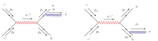
Figure 1: Feynman diagrams for the real emission of a gluon from the final state quark or anti-quark.

It is standard practice to define the dimensionless energy fractions for the final state particles,

$$x_{i}\,=\,\frac{2E_{i}}{Q}\quad\quad(i=1,2,3)\,,$$ (8)

where $Q$ is the total center of mass energy, with $x_{1}+x_{2}+x_{3}\,=\,2$. One can readily derive the relations

$$(p_{2}+p_{3})^{2}\,=\, 2p_{2}\cdotp p_{3}\,=\,Q^{2}(1-x_{1}),$$

$$(p_{1}+p_{3})^{2}\,=\, 2p_{1}\cdotp p_{3}\,=\,Q^{2}(1-x_{2}),$$ (9)

$$(p_{1}+p_{2})^{2}\,=\, 2p_{1}\cdotp p_{2}\,=\,Q^{2}(1-x_{3}),$$

using momentum conservation. For a final state with three massless particles, eq. (5) takes the simple form

$$T\,=\,\text{max}(x_{1},x_{2},x_{3})\,.$$ (10)

III.1 Thrust distribution at NLO

The thrust distribution at NLO is given by

$$\frac{d\sigma}{dT}\,=\,\frac{1}{2s}\int d\Phi_{3}\overline{\sum}|\mathcal{M}(x_{1},x_{2})|^{2}\delta(T-\text{max}(x_{1},x_{2},x_{3})),$$ (11)

where $s$ is the center of mass energy squared. The matrix element squared for the process in eq. (7) is

$$\overline{\sum} |\mathcal{M}(x_{1},x_{2})|^{2}$$

$$\,=\, 8(e^{2}e_{q})^{2}g_{s}^{2}C_{F}N_{c}\frac{1}{3Q^{2}}\,\frac{x_{1}^{2}+x_{2}^{2}}{(1-x_{1})(1-x_{2})}\,,$$ (12)

where $\alpha=\left(e^{2}/4\pi\right)$, $e_{q}$ is the charge of quarks in the unit of fundamental electric charge $e$, $\alpha_{s}=g_{s}^{2}/4\pi$, $C_{F}=(N_{c}^{2}-1)/2N_{c}$, and $N_{c}$ is the number of quark colours. The three-particle phase space measure, expressed in terms of $x_{i}$ reads

$$d\Phi_{3}\,=\, \frac{Q^{2}}{16(2\pi)^{3}}\,dx_{1}\,dx_{2}\,dx_{3}\,\delta(x_{1}+x_{2}+x_{3}-2).$$ (13)

The phase space in eq. (13) is depicted in fig. (2),

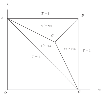
Figure 2: The Dalitz plot for the production of three massless particles. The phase space can be divided into three different regions depending upon which energy fraction is the largest. In region ABG, $x_{1}$ is the largest of the three $x_{i}$, while in region BGC, (AGC) $x_{2}$ ($x_{3}$) is the largest. In this figure, we set $BA=BC=1$. Along the lines AB, BC, and AC one has $T=1$.

with every point in the plane fulfilling the constraint $x_{1}+x_{2}+x_{3}=2$. The region surrounding point $A$ ($C$) corresponds to the soft anti-quark (quark) region, and the region around $B$ to the soft gluon region. On line $BA$, where $x_{1}=1$, the anti-quark and gluon move collinearly in opposite directions, while on line $BC$, where $x_{2}=1$, the quark and the gluon are collinear. On line $AC$, where $x_{3}=1$, the quark and the anti-quark are collinear, with the gluon moving in the opposite direction. Along these three lines, $T=1$.

To obtain the thrust distribution one integrates over the $x_{1},x_{2}$ variables in eq. (11) with the appropriate limits:

$$\frac{1}{\sigma_{0}(s)}\frac{d\sigma}{dT}\,=\,\frac{2\alpha_{s}}{3\pi}\int_{0}^{1}dx_{1}\int_{0}^{1-x_{1}} dx_{2}\,\,\frac{x_{1}^{2}+x_{2}^{2}}{(1-x_{1})(1-x_{2})}$$

$$\times\delta\left(T-\text{max}(x_{1},x_{2},x_{3})\right)\,,$$ (14)

where $x_{3}=2-x_{1}-x_{2}$, and $\sigma_{0}(s)$ is the LO cross-section, given by

$$\sigma_{0}(s)\,=\,\frac{4\pi\alpha^{2}e_{q}^{2}\,N_{c}}{3s}\,,$$ (15)

For our purposes, we label the contributions from three distinct contributions in the phase space integration in eq. (III.1), defined by either $x_{1}$, $x_{2}$, and $x_{3}$ being the largest, as follows:

1. Quark has the largest energy ($x_{1}>x_{2},x_{3}$)

2. Anti-quark has the largest energy ($x_{2}>x_{1},x_{3}$)

3. Gluon has the largest energy ($x_{3}>x_{1},x_{2}$)

The contribution from region I is then

$$\frac{1}{\sigma_{0}(s)}\frac{d\sigma}{dT}{\Bigg{|}_{\text{I}}}\,=\,\frac{2\alpha_{s}}{3\pi}\int_{0}^{1}dx_{2}\int_{0}^{1-x_{2}}dx_{1}\, \frac{x_{1}^{2}+x_{2}^{2}}{(1-x_{1})(1-x_{2})}\,\,$$

$$\times \delta(T-x_{1})\,.$$ (16)

With the appropriate limits of integration we have

$$\frac{1}{\sigma_{0}(s)}\frac{d\sigma}{dT}{\Bigg{|}_{\text{I}}}\,=\,\frac{2\alpha_{s}}{3\pi}\int_{2(1-T)}^{T}dx_{2}\,\frac{T^{2}+x_{2}^{2}}{(1-T)(1-x_{2})}.$$ (17)

Instead of $T$, we shall mostly use the variable $\tau\,=\,1-T$, which vanishes in the zero-radius dijet limit. The integration in eq. (17) leads to

$$\frac{1}{\sigma_{0}(s)}\frac{d\sigma}{d\tau}{\Bigg{|}_{\text{I}}}$$

$$\,=\, \ \frac{2\alpha_{s}}{3\pi}\biggl{[}\frac{3\tau^{2}+8\tau-3}{2\tau}+\left(\frac{\tau^{2}-2\tau+2}{\tau}\right)\log\left(\frac{1-2\tau}{\tau}\right)\biggr{]}.$$ (18)

Expanding the above expression around $\tau=0$ gives

$$\frac{1}{\sigma_{0}(s)}\frac{d\sigma}{d\tau}{\Bigg{|}_{\text{I}}}$$

$$=\ \frac{2\alpha_{s}}{3\pi}\biggl{(}\frac{-3-4\log\tau}{2\tau}+2\log\tau+\frac{3\tau}{2}-\tau\log\tau+\mathcal{O}(\tau^{2})\biggr{)}.$$ (19)

The first term in the brackets forms the LP term (in $\tau$), with both leading-logarithmic (LL) and next-to-leading logarithmic (NLL) terms. The former derives from soft and collinear gluon emission, the latter from hard collinear gluon emission. The next term constitutes the (NLP) term, which is our main focus here. Subsequent terms are of NNLP and beyond accuracy. The result for thrust distribution from region I is provided in eq. (19); however, this expression does not show the correspondence between the various kinematical configurations and the contributions they produce at the LP and NLP. In order to extract such information, we shall split the integration result of eq. (17) into its upper and lower limit contributions separately, as these limits reflect the different regions of the phase space. The contributions from the upper (I,u) and lower (I,l) limits of $x_{2}$ from the region I are, respectively, after expansion around $\tau\,=\,0$

$$\frac{1}{\sigma_{0}(s)}\frac{d\sigma}{d\tau}{\Bigg{|}_{\text{I,u}}}$$

$$= \ \frac{2\alpha_{s}}{3\pi}\biggl{(}\frac{-2\log\tau}{\tau}+2+2\log\tau-\frac{\tau}{2}+\tau\log\tau+\mathcal{O}\left(\tau^{2}\right)\biggr{)},$$ (20)

$$\frac{1}{\sigma_{0}(s)}\frac{d\sigma}{d\tau}{\Bigg{|}_{\text{I,l}}}\,=\, \ \frac{2\alpha_{s}}{3\pi}\left(\frac{3}{2\tau}+2-2\tau+\mathcal{O}(\tau^{2})\right).$$ (21)

Note that here and henceforth the lower limit term is to be subtracted from the upper limit result. In region I, the upper limit of $x_{2}$ for small $\tau$ corresponds to a back-to-back quark and anti-quark configuration allowing the gluon to go soft while the lower limit corresponds to the quark and gluon being back-to-back, allowing the gluon to be hard. The LL terms at LP and NLP follow only from the upper limit ($x_{2}\,=\,1-\tau$), whereas the lower limit ($x_{2}\,=\,2\tau$) yields NLL terms both at LP and NLP. In fact, identical NLL contributions at NLP follow from both limits; they therefore cancel in the final result for region I.

Thus the upper and lower limit contributions unveil the relation between the particular kinematical configurations and their respective contributions at LP and NLP. To better comprehend the origin of LP and NLP terms, we will from here on first provide our full results and then their breakdown into upper and lower limit contributions.

In region II, due to the symmetry under the interchange of $x_{1}\leftrightarrow x_{2}$, the contribution from this region is identical to eq. (19). Thus

$$\frac{1}{\sigma_{0}(s)}\frac{d\sigma}{d\tau}{\Bigg{|}_{\text{II}}}\,=\,\frac{1}{\sigma_{0}(s)}\frac{d\sigma}{d\tau}{\Bigg{|}_{\text{I}}}\,.$$ (22)

In region III, the thrust axis is aligned with the momentum of the gluon. The contribution is

$$\frac{1}{\sigma_{0}(s)}\frac{d\sigma}{dT}{\Bigg{|}_{\text{III}}}\,=\,\frac{2\alpha_{s}}{3\pi}\int_{0}^{1}dx_{2} \int_{0}^{1-x_{2}}dx_{1}\,\frac{x_{1}^{2}+x_{2}^{2}}{(1-x_{1})(1-x_{2})}\,\,$$

$$\times\delta(T+x_{1}+x_{2}-2)\,,$$ (23)

which gives

$$\frac{1}{\sigma_{0}(s)}\frac{d\sigma}{dT}{\Bigg{|}_{\text{III}}}\,=\,\frac{2\alpha_{s}}{3\pi}\int_{2(1-T)}^{T}dx_{2}\,\frac{(2-x_{2}-T)^{2}+x_{2}^{2}}{(x_{2}+T-1)(1-x_{2})}\,.$$ (24)

Expanding in $\tau$ gives

$$\frac{1}{\sigma_{0}(s)}\frac{d\sigma}{d\tau}{\Bigg{|}_{\text{III}}}$$

$$\,=\,\ \frac{2\alpha_{s}}{3\pi}\bigg{(}-2-2\log{\tau}+(2-2\log\tau)\tau+\mathcal{O}(\tau^{2})\bigg{)}.$$ (25)

Thus no LP contributions arise from region III, as expected. The $\tau=0$ configurations in this region correspond to either the quark or anti-quark being soft, or the quark and anti-quark pair moving collinearly opposite to the gluon. The latter configuration does not lead to a large contribution because the propagator is then far off the mass-shell. The contribution from upper and lower limits from this region respectively are, for small $\tau$,

$$\frac{1}{\sigma_{0}(s)} \frac{d\sigma}{d\tau}{\Bigg{|}_{\text{III,u}}}$$

$$\,=\, \ \frac{2\alpha_{s}}{3\pi}\biggl{(}-2-\log\tau+(1-\log\tau)\tau+\mathcal{O}\left(\tau^{2}\right)\biggr{)},$$ (26)

$$\frac{1}{\sigma_{0}(s)}\frac{d\sigma}{d\tau}{\Bigg{|}_{\text{III,l}}}\,=\,\ \frac{2\alpha_{s}}{3\pi}\bigg{(}\log\tau+(-1+\log\tau)\tau+\mathcal{O}(\tau^{2})\bigg{)}.$$ (27)

The upper limit of $x_{2}$ in region III corresponds to the gluon and anti-quark being back-to-back, and the lower limit has the gluon and quark back-to-back. LL terms at NLP arise from both limits.

Combining contributions from all three regions, the thrust distribution at NLO yields the well-known result

$$\frac{1}{\sigma_{0}(s)}\frac{d\sigma}{d\tau}\Bigg{|}_{\text{NLO}}\,=\,\frac{2\alpha_{s}}{3\pi} \biggl{[}\frac{2(3\tau^{2}-3\tau+2)}{\tau(1-\tau)}\,\log\left(\frac{1-2\tau}{\tau}\right)$$

$$\hskip 42.67912pt-\frac{3(1-3\tau)(1+\tau)}{\tau}\biggr{]}\,,$$ (28)

with expansion

$$\frac{1}{\sigma_{0}(s)}\frac{d\sigma}{d\tau}\Bigg{|}_{\text{NLO}}\,=\,\ \frac{2\alpha_{s}}{3\pi} \biggl{(}\frac{-3-4\log{\tau}}{\tau}-2+2\log{\tau}+(5\tau$$

$$\hskip 42.67912pt-4\log\tau)\tau+\mathcal{O}(\tau^{2})\biggr{)}.$$ (29)

Note that in eq. (29) at NLP all three regions produce LL terms, but a partial cancellation takes place when combined.

III.2 Next-to-leading power corrections for thrust from kinematical shifts

Next we use the method of kinematical shifts [92, 46] to compute dominant NLP terms for the thrust distribution due to gluon radiation. The expression for the shifted matrix elements is given in eq. (3), with the momenta shifts given by eq. (4). Note that because the emitted gluon is emitted from final particles the momenta shifts in eq. (3) are subtracted [46] from the radiating particle momenta, rather than added as for the initial state case. The squared, spin-summed, and averaged LO matrix element $|\mathcal{M}_{0}|^{2}$ for the process in eq. (6) is

$$\overline{\sum}|\mathcal{M}_{0}(p_{1},p_{2})|^{2}\,=\,\frac{4(e^{2}e_{q})^{2}N_{c}}{3s}(2p_{1}\cdot p_{2})\,.$$ (30)

Inserting shifted momenta according to eq. (4) leads to

$$\overline{\sum} |\mathcal{M}_{0}(p_{1}-\delta p_{1},p_{2}-\delta p_{2})|^{2}$$

$$\,=\, \frac{8(e^{2}e_{q})^{2}N_{c}}{3Q^{2}}\biggl{[}(p_{1}\cdot p_{2})+p_{3}\cdot(p_{1}+p_{2})+{\cal O}(p_{3}^{2})\biggr{]}\,.$$ (31)

The last term contains two powers of the momentum $p_{3}$, and can thus be omitted. Combining eqs. (3) and (31) gives the expression for shifted matrix element squared as

$$\overline{\sum} |{\mathcal{M}}_{\text{shift}}|^{2}$$

$$\,=\, 8(e^{2}e_{q})^{2}N_{c}C_{F}g_{s}^{2}\,\frac{1}{3Q^{2}}\,$$

$$\times\left(\frac{2(p_{1}\cdot p_{2})^{2}}{(p_{1}\cdot p_{3})(p_{2}\cdot p_{3})}+\frac{2p_{1}\cdot p_{2}}{p_{2}\cdot p_{3}}+\frac{2p_{1}\cdot p_{2}}{p_{1}\cdot p_{3}}\right)\,,$$ (32)

which, expressed in terms of $x_{i}$’s, reads

$$\overline{\sum}|{\mathcal{M}}_{\text{shift}}(p_{1},p_{2})|^{2}\,=\, 8(e^{2}e_{q})^{2}N_{c}g_{s}^{2}C_{F}\,\frac{1}{3Q^{2}}\,$$

$$\hskip 14.22636pt\times\left(\frac{2x_{1}+2x_{2}-2}{(1-x_{1})(1-x_{2})}\right)\,.$$ (33)

Note that when the emitted gluon becomes soft (i.e. $x_{1},x_{2}\to 1$), the above matrix element diverges, whereas when the gluon is hard ($x_{3}\to 1$), the numerator $(2x_{1}+2x_{2}-2)$ vanishes. The thrust distribution under this approximation is given by

$$\frac{d\sigma}{dT}\Bigg{|}_{\text{shift}}\,=\,\frac{1}{2s}\int d\Phi_{3}\,\, \overline{\sum}\ |\mathcal{M}_{\text{shift}}(x_{1},x_{2})|^{2}\,\,$$

$$\times\delta(T-\text{max}(x_{1},x_{2},x_{3})).$$ (34)

We repeat the steps to compute the thrust distribution from the exact computation for each of the three regions. Region I gives

$$\frac{1}{\sigma_{0}(s)}\frac{d\sigma}{dT}{\Bigg{|}_{\text{I}}}\,=\,\frac{2\alpha_{s}}{3\pi}\int_{0}^{1}dx_{2}\int_{0}^{1-x_{2}}dx_{1}\,\, \frac{2x_{1}+2x_{2}-2}{(1-x_{1})(1-x_{2})}\,\,$$

$$\times\delta(T-x_{1}),$$ (35)

which leads to the expansion about $\tau\,=\,0$

$$\frac{1}{\sigma_{0}(s)}\frac{d\sigma}{d\tau}{\Bigg{|}_{\text{I}}}$$

$$\,=\,\ \frac{2\alpha_{s}}{3\pi}\left(\frac{-2-2\log\tau}{\tau}+2+2\log\tau+\mathcal{O}(\tau^{2})\right).$$ (36)

When we compare the above expression to eq. (19), we see that the LLs at both the LP and NLP are correctly captured, while the NLL terms at LP are only partially reproduced. The contributions from upper and lower limits are

$$\frac{1}{\sigma_{0}(s)}\frac{d\sigma}{d\tau}{\Bigg{|}_{\text{I,u}}}\,=\, \ \frac{2\alpha_{s}}{3\pi}\left[-\frac{2(1-\tau)(1+\log\tau)}{\tau}\right],$$ (37)

$$\frac{1}{\sigma_{0}(s)}\frac{d\sigma}{d\tau}{\Bigg{|}_{\text{I,l}}}\,=\, \ \frac{2\alpha_{s}}{3\pi}\left[-4-\frac{2(1-\tau)\log(1-2\tau)}{\tau}\right],$$ (38)

which, expanded around $\tau\,=\,0$, gives

$$\frac{1}{\sigma_{0}(s)}\frac{d\sigma}{d\tau}{\Bigg{|}_{\text{I,u}}}\,=\,\ \frac{2\alpha_{s}}{3\pi}\biggl{(}\frac{-2-2\log\tau}{\tau}+2+ 2\log\tau$$

$$+\mathcal{O}(\tau^{2})\biggr{)},$$ (39)

$$\frac{1}{\sigma_{0}(s)}\frac{d\sigma}{d\tau}{\Bigg{|}_{\text{I,l}}}\,=\, \ \frac{2\alpha_{s}}{3\pi}\bigg{(}\mathcal{O}(\tau^{2})\bigg{)}.$$ (40)

The upper limit contribution in region I contains the LL and NLL terms at LP and NLP, while the lower limit acts beyond NLP. The contribution from region II is identical to I. The contribution from region III is

$$\frac{1}{\sigma_{0}(s)}\frac{d\sigma}{dT}{\Bigg{|}_{\text{III}}}\,=\frac{2\alpha_{s}}{3\pi}\int_{0}^{1}dx_{2} \int_{0}^{1-x_{2}}dx_{1}\,\,$$

$$\times\delta (T+x_{1}+x_{2}-2)$$

$$\times \frac{2x_{1}+2x_{2}-2}{(1-x_{1})(1-x_{2})}\,,$$ (41)

which gives

$$\frac{1}{\sigma_{0}(s)}\frac{d\sigma}{d\tau}{\Bigg{|}_{\text{III}}}\,=\,\ \frac{2\alpha_{s}}{3\pi}\left[\frac{4\tau}{1-\tau}\log\left(\frac{1-2\tau}{\tau}\right)\right]\,.$$ (42)

Upon expansion around $\tau\,=\,0$ this yields only terms beyond NLP accuracy

$$\frac{1}{\sigma_{0}(s)}\frac{d\sigma}{d\tau}{\Bigg{|}_{\text{III}}}\,=\,\ \frac{2\alpha_{s}}{3\pi}\bigg{(}-4\tau\log\tau+\mathcal{O}(\tau^{2})\bigg{)}\,,$$ (43)

$$\frac{1}{\sigma_{0}(s)}\frac{d\sigma}{d\tau}{\Bigg{|}_{\text{III,u}}} \,=\,\ \frac{2\alpha_{s}}{3\pi}\bigg{(}-2\tau\log\tau+\mathcal{O}(\tau^{2})\bigg{)},$$ (44)

$$\frac{1}{\sigma_{0}(s)}\frac{d\sigma}{d\tau}{\Bigg{|}_{\text{III,l}}} \,=\,\ \frac{2\alpha_{s}}{3\pi}\bigg{(}2\tau\log\tau+\mathcal{O}(\tau^{2})\bigg{)}\,.$$ (45)

Indeed the hard gluon/soft quark region is not part of the shifted kinematics method.

Combining contributions from all three regions the thrust distribution from shifted kinematics formalism at NLO reads

$$\frac{1}{\sigma_{0}(s)}\frac{d\sigma}{d\tau}\Bigg{|}_{\text{shift}}\,=\,\frac{2\alpha_{s}}{3\pi}\biggl{[}\frac{8\tau^{2}-8\tau+4}{\tau(1-\tau)} \log\left(\frac{1-2\tau}{\tau}\right)$$

$$-\frac{3\tau^{2}-4\tau+1}{\tau(1-\tau)}\biggr{]}\,,$$ (46)

or

$$\frac{1}{\sigma_{0}(s)}\frac{d\sigma}{d\tau}\Bigg{|}_{\text{shift}}\,=\,\ \frac{2\alpha_{s}}{3\pi} \bigg{[}\frac{-4-4\log{\tau}}{\tau}+4+4\log{\tau}$$

$$\hskip 25.6073pt-(4\log\tau)\tau+\mathcal{O}(\tau^{2})\bigg{]}.$$ (47)

When compared to the exact computation in eq. (29), we see that the LL terms at LP have been reproduced, in addition to some NLL terms. At the NLP level, we have captured some, but not all, of the LL terms, in addition to some NLL contributions. The missing LL terms at NLP should arise from soft quark (anti-quark) contributions.

The exact squared matrix element in eq. (12) has the following $x_{i}$ dependence

$$\overline{\sum}|{\mathcal{M}}(x_{1},x_{2})|^{2}\,=\,8(e^{2}e_{q})^{2}N_{c}C_{F}g_{s}^{2}\frac{1}{3Q^{2}}\,\biggl{(}\frac{2}{(1-x_{1})(1-x_{2})}-\frac{2}{1-x_{1}}-\frac{2}{1-x_{2}}+\frac{1-x_{2}}{1-x_{1}}+\frac{1-x_{1}}{1-x_{2}}\biggr{)}.$$ (48)

The first three terms constitute the shifted matrix element squared, as shown in eq. (33). The eikonal approximation in fact consists of only the first term of eq. (48). The remaining last two terms in eq. (48) we refer to as remainder matrix element squared and it has following form

$$\overline{\sum} |{\mathcal{M}}_{\text{rem}}(x_{1},x_{2})|^{2}$$

$$\,=\,8(e^{2}e_{q})^{2}N_{c}C_{F}g_{s}^{2}\frac{1}{3Q^{2}}\biggl{(}\frac{1-x_{2}}{1-x_{1}}+\frac{1-x_{1}}{1-x_{2}}\biggr{)}\,.$$ (49)

Let us take the first term on the right, which diverges for $x_{1}\to 1$. It is most relevant when $x_{2}\to 0$ and $x_{1}\to 1$, i.e. $x_{3}\to 1$, which corresponds to the emission of a soft anti-quark. Similarly the second term is dominant when $x_{1}\to 0$ and $x_{2}\to 1$ i.e. the emission of soft quark.

The contributions from soft quark and anti-quark emissions can alternatively be computed using the quark emission operator defined in [46]. The matrix element for the emission of a soft quark ($p_{1}\to 0$) in fig. (1) is

$$i\mathcal{M}_{1,q}\,=\, \frac{ig_{s}t_{a}}{2p_{1}\cdot p_{3}}\left[\mathcal{M}_{H_{1}}(p_{1},p_{2},p_{3})\not{p}_{3}\gamma^{\mu}\bar{\epsilon}_{\mu}\bar{u}(p_{1})\right]\,,$$ (50)

and similarly for the emission of soft anti-quark ($p_{2}\to 0$)

$$i\mathcal{M}_{2,q}\,=\, \frac{ig_{s}t_{a}}{2p_{2}\cdot p_{3}}\left[\mathcal{M}_{H_{2}}(p_{1},p_{2},p_{3})\not{p}_{3}\gamma^{\mu}\bar{\epsilon}_{\mu}v(p_{2})\right]\,.$$ (51)

Here the hard scattering matrix elements $\mathcal{M}_{H_{1}}$ and $\mathcal{M}_{H_{2}}$ are defined to contain all the external states except for the polarization vector $\epsilon_{\mu}$ and spinors for soft fermion emission. The matrix element squared after the sum (average) over the final (initial) state spins and colours

$$\overline{\sum} |\mathcal{M}_{q}|^{2}\,=\,\overline{\sum}|{\mathcal{M}}_{\text{rem}}(x_{1},x_{2})|^{2}\,$$

$$=\,8(e^{2}e_{q})^{2}N_{c}C_{F}g_{s}^{2}\frac{1}{3Q^{2}}\left(\frac{1-x_{2}}{1-x_{1}}+\frac{1-x_{1}}{1-x_{2}}\right)\,,$$ (52)

which indeed reproduces eq. (49). Thus eq. (49) features a clean separation of the soft quark and anti-quark contributions from the next-to-soft gluon contributions. Soft quark emissions contribute to the LL terms at NLP [46]. Their contribution to the thrust distribution from region I is

$$\frac{1}{\sigma_{0}(s)}\frac{d\sigma}{dT}{\Bigg{|}_{\text{I}}}\,=\,\frac{2\alpha_{s}}{3\pi}\int_{0}^{1}dx_{2}\int_{0}^{1-x_{2}} dx_{1}\,\,\delta(T-x_{1})$$

$$\times \left(\frac{1-x_{1}}{1-x_{2}}+\frac{1-x_{2}}{1-x_{1}}\right)\,\,,$$ (53)

which gives

$$\frac{1}{\sigma_{0}(s)}\frac{d\sigma}{d\tau}{\Bigg{|}_{\text{I}}}\,=\,\ \frac{2\alpha_{s}}{3\pi}\left(\frac{1}{2\tau}-2+\frac{3\tau}{2}-\tau\log\tau+\mathcal{O}(\tau^{2})\right).$$ (54)

The upper and lower limit components are

$$\frac{1}{\sigma_{0}(s)}\frac{d\sigma}{d\tau}{\Bigg{|}_{\text{I,u}}} \,=\,\ \frac{2\alpha_{s}}{3\pi}\bigg{(}\frac{1}{2\tau}+-\frac{\tau}{2}-\tau\log\tau+\mathcal{O}(\tau^{2})\bigg{)},$$ (55)

$$\frac{1}{\sigma_{0}(s)}\frac{d\sigma}{d\tau}{\Bigg{|}_{\text{I,l}}} \,=\,\ \frac{2\alpha_{s}}{3\pi}\bigg{(}2-2\tau+\mathcal{O}(\tau^{2})\bigg{)}\,.$$ (56)

In this region, the hard gluon can become collinear to the anti-quark, and the contribution from this kinematical configuration is captured by the upper limit of $x_{2}$, which yields the NLL at LP. At the same time, the lower limit captures the NLL at NLP. Region II again gives a contribution identical to eq. (54). Region III gives

$$\frac{1}{\sigma_{0}(s)}\frac{d\sigma}{dT}{\Bigg{|}_{\text{III}}}\,=\,\frac{2\alpha_{s}}{3\pi}\int_{0}^{1}dx_{2} \int_{0}^{1-x_{2}}dx_{1}$$

$$\times\left(\frac{1-x_{1}}{1-x_{2}}+\frac{1-x_{2}}{1-x_{1}}\right)\,\,$$

$$\times\delta(T+x_{1}+x_{2}-2),$$ (57)

$$\frac{1}{\sigma_{0}(s)}\frac{d\sigma}{d\tau}{\Bigg{|}_{\text{III}}}\,=\,\ \frac{2\alpha_{s}}{3\pi}\bigg{(}-2-2\log\tau+ 2(1+\log\tau)\tau$$

$$+\mathcal{O}(\tau^{2})\bigg{)}.$$ (58)

The contributions from upper and lower limits are

$$\frac{1}{\sigma_{0}(s)}\frac{d\sigma}{d\tau}{\Bigg{|}_{\text{III,u}}} \,=\, \frac{2\alpha_{s}}{3\pi}\bigg{(}-2-\log\tau-\tau\log\tau+\mathcal{O}(\tau^{2})\bigg{)},$$ (59)

$$\frac{1}{\sigma_{0}(s)}\frac{d\sigma}{d\tau}{\Bigg{|}_{\text{III,l}}} \,=\, \frac{2\alpha_{s}}{3\pi}\bigg{(}\log\tau+(-2-\log\tau)\tau+\mathcal{O}(\tau^{2})\bigg{)}.$$ (60)

As the upper limit corresponds to soft quark emission and the lower limit to soft anti-quark contributions, one finds LL contributions at NLP from both limits. The remained matrix element squared in region III reproduces the missing LL contributions at NLP in eq. (47), which the shifted kinematics methods do not capture.

$$\frac{1}{\sigma_{0}(s)}\frac{d\sigma}{d\tau}{\Bigg{|}_{\text{rem}}}\,=\,\ \frac{2\alpha_{s}}{3\pi}\bigg{(}\frac{1}{\tau}-6-2\log\tau+5\tau\bigg{)}.$$ (61)

These are, as expected, the terms that were missing from eq. (47). It is now interesting to assess the quality of the shifted kinematics approximation.

III.3 Numerical assessment of the shifted kinematics approximations for thrust

The shifted kinematics approximation at the cross-section level changes the Born cross-section $\sigma_{0}(s)$ in eq. (15) by replacing $s\to s(1-\tau)^{-1}$

$$\sigma_{0}\left(\frac{s}{1-\tau}\right)\,=\,\sigma_{0}(s)(1-\tau).$$ (62)

The LP term of thrust distribution computed under the formalism of shifted kinematics in eq. (47) is

$$\frac{d\sigma}{d\tau}\Bigg{|}_{\text{LP}}\,=\,\ \frac{2\alpha_{s}}{3\pi}\left(\frac{-4-4\log\tau}{\tau}\right)\sigma_{0}(s),$$ (63)

when multiplied by the shifted born cross-section in eq. (62) yields

$$\sigma_{0} \left(\frac{s}{1-\tau}\right)\,\times\frac{d\sigma}{d\tau}\Bigg{|}_{\text{LP}}$$

$$\,=\,\ \frac{2\alpha_{s}}{3\pi}\biggl{(}\frac{-4-4\log{\tau}}{\tau}+4+4\log{\tau}\biggr{)}\sigma_{0}(s)\,.$$ (64)

which reproduces eq. (47). In fig. (3a) we compare the thrust distribution as computed from the shifted kinematics approximation in eq. (47), up to NLP, with the exact computation in eq. (28).

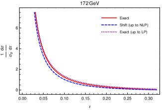
(a)

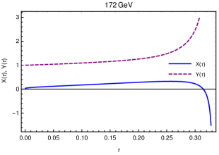
(b)

Figure 3: In (a), we plot comparison of the thrust distribution. We show the exact result (solid red curve) in eq. (28), the shifted approximation (dashed blue curve) up to NLP terms given in eq. (47). We also plot the exact LP term (dotted purple curve). In (b), we show $X(\tau)$ in eq. (65) (solid blue curve) and $Y(\tau)$ in eq. (66) (purple dashed curve) vs. $\tau$.

In the small $\tau$ region, the LP terms alone provide an excellent approximation to the exact result. However, as $\tau$ increases, we notice that the shifted kinematic curve approximates the exact results better. The reason LP terms are such an excellent approximation for thrust is the small coefficient of the NLP LL term; as such the NLL at LP for thrust dominates the LL term at NLP for small values of $\tau$. This is, as we shall see, in contrast to the $C$-parameter, the LL at NLP dominates the NLL term at LP [99, 100] in the dijet limit.

In fig. (3b) we provide two different ratio plots that involve expressions of thrust distribution computed from both of the approaches viz. the exact approach (28) and the shifted approach (47). We define $X(\tau)$ and $Y(\tau)$ as

$$X(\tau)\,=\, \frac{\frac{1}{\sigma_{0}(s)}\frac{d\sigma}{d\tau}\Big{|}_{\text{NLO}}-\frac{1}{\sigma_{0}(s)}\frac{d\sigma}{d\tau}\Big{|}_{\text{shift-NLP}}}{\frac{1}{\sigma_{0}(s)}\frac{d\sigma}{d\tau}\Big{|}_{\text{NLO}}},$$ (65)

$$Y(\tau)\,=\, \frac{\frac{1}{\sigma_{0}(s)}\frac{d\sigma}{d\tau}\Big{|}_{\text{NLO-LP}}}{\frac{1}{\sigma_{0}(s)}\frac{d\sigma}{d\tau}\Big{|}_{\text{NLO}}}.$$ (66)

As is evident from their expressions, $X(\tau)$ measures the accuracy of the shifted approximation, whereas $Y(\tau)$ measures the importance of NLP terms (and beyond) compared to the LP terms. The plot of $X(\tau)$ shows that the shifted kinematics method approximates the exact result well near the dijet limit. The plot of $Y(\tau)$ shows that the LP contribution is dominant near $\tau\to 0$. As $\tau$ increases, the denominator falls faster than the numerator due to the presence of the NLP terms in addition to the LP contribution, and thus the ratio rises above one.

IV $C$-parameter

In the previous section, we compared the shifted kinematic approximation of the thrust distribution with the exact NLO result, to understand the origin of NLP corrections. Here we perform the same comparison for the more complicated $C$-parameter distribution. The $C$-parameter for massless particles [101, 102, 103, 104] is defined as

$$C\,=\,3-\frac{3}{2}\sum_{i,\ j}\frac{\left(p_{i}\cdot p_{j}\right)^{2}}{\left(p_{i}\cdot q\right)\left(p_{j}\cdot q\right)}\,,$$ (67)

where $p_{i}$ is the four-momentum of $i$-th particle, the total four-momentum is given by $q=\sum_{i}p_{i}$, and the sums over $i$ and $j$ run over all the particles present in the final state. The minimum value taken by $C$ equals $0$ (for a zero-radius dijet event), and the maximum value is $1$ (for an isotropic event). Here we consider a three-body final state, for which the maximal value of $C$ is $3/4$; the value $C=1$ can only be obtained if more than three particles are present in the final state. For the three-body final state in fig. (1), it takes the form

$$C\,=\,\frac{6\left(1-x_{1}\right)\left(1-x_{2}\right)\left(1-x_{3}\right)}{x_{1}\ x_{2}\ x_{3}}\,,$$ (68)

where $x_{i}$ are the energy fractions given in eq. (9). The $C$-parameter has a critical point at $C=3/4$, which gives rise to a Sudakov shoulder [105]. However, these first occur at second order in $\alpha_{s}$, where four-particle final states are possible, hence our study does not encounter them. Henceforth we work with a rescaled definition of the $C$-parameter

$$c\,=\,\frac{C}{6}\,=\,\frac{\left(1-x_{1}\right)\left(1-x_{2}\right)\left(1-x_{3}\right)}{x_{1}\ x_{2}\ x_{3}}\,,$$ (69)

for which the range is $0<c<1/8$. Note that the definition of the $c$-parameter does not involve the selection of a special axis, which thereby distinguishes it from a group of other event shapes variables such as thrust, jet broadening, jet mass, and angularities.

IV.1 The $c$-parameter distribution at NLO

The $c$-parameter distribution is defined as

$$\frac{d\sigma}{dc}\,=\,\frac{1}{2s}\int d\Phi_{3}\ \overline{\sum}\ |\mathcal{M}(x_{1},x_{2})|^{2}\ \delta\left(c(x_{1},x_{2})-c\right),$$ (70)

where $\overline{\sum}\ |\mathcal{M}(x_{1},x_{2})|^{2}$ and $d\Phi_{3}$ are given in eq. (12) and eq. (13) respectively. The normalized expression at NLO takes the form

$$\frac{1}{\sigma_{0}(s)}\frac{d\sigma}{dc}\,=\,\ \frac{2\alpha_{s}}{3\pi}\int_{0}^{1}dx_{1}\int_{0}^{1-x_{1}} dx_{2}\ \frac{x_{1}^{2}+x_{2}^{2}}{(1-x_{1})(1-x_{2})}$$

$$\times\delta\left(c(x_{1},x_{2})-c\right).$$ (71)

The integrations over energy fractions are considerably more involved than for thrust due to the rational polynomial form in eq. (69). It is advantageous to convert our kinematic variables to $(y,z)$ [100] where

$$y\,=\, 2-x_{1}-x_{2},$$

$$z\,=\, \frac{1-x_{2}}{y}\,,$$ (72)

with Jacobian $J(z,y)=y$. Note that $y$ is in fact the gluon energy fraction. The expressions for the matrix element and $c$-parameter in terms of the new variables read

$$\overline{\sum}\ |{\mathcal{M}(y,z)}|^{2}$$

$$\,=\,8(e^{2}e_{q})^{2}N_{c}C_{F}g_{s}^{2}\frac{1}{3Q^{2}}\left(\frac{2+y(y-2yz(1-z)-2)}{y^{2}z(1-z)}\right),$$ (73)

and

$$c(y,z)\,=\,\frac{(1-y)(1-z)yz}{(1-y(1-z))(1-yz)}\,.$$ (74)

The $x_{1}\leftrightarrow x_{2}$ symmetry in the matrix element squared in eq. (12) now appears as $z\leftrightarrow(1-z)$ symmetry in eq. (73). Substitution into eq. (70) yields

$$\frac{1}{\sigma_{0}(s)} \frac{d\sigma}{dc}\Bigg{|}_{\text{NLO}}$$

$$\,=\,\frac{2\alpha_{s}}{3\pi}\int^{1}_{0}dy\ \int^{1}_{0}dz\ \frac{2+y(y-2yz(1-z)-2)}{yz(1-z)}\$$

$$\hskip 85.35826pt\times\delta\left(c(y,z)-c\right).$$ (75)

To determine the limits of the $z$-integration, we use the phase space in fig. (2) as follows. From eq. (72), it is evident that $z$ will attain its lowest value when $x_{2}=1$, yielding $z=0$ as the lower limit of $z$. Similarly, $z$ will attain its largest value when $x_{2}$ and $y$ both are smallest. However $x_{2}$ and $y$ cannot be zero at the same time. Thus with $x_{2}\to 0$ (and thus $y\to 1$), one finds that $z=1$ is the upper limit. The limits of the $y$-integration can be found from the $\delta$-function constraint and the limits of the $z$-integration. We first rewrite eq. (75) in the form

$$\frac{1}{\sigma_{0}(s)}\frac{d\sigma}{dc}\Bigg{|}_{\text{NLO}}\,=\,\frac{2\alpha_{s}}{3\pi}\int^{1}_{0}dy\int^{1}_{0}dz\frac{2(y(z-1)+1)^{2}(yz-1)^{2}(y(2y(z-1)z+y-2)+2)}{(y-1)^{2}y^{2}(z-1)z(2z-1)}\biggl{(}\delta(z-z_{1})+\delta(z-z_{2})\biggr{)}\,,$$ (76)

where we used the argument of the $\delta$-function in eq. (75) and it has following two roots

$$z_{1,2} \,=\,\frac{1}{2}\left(1\pm\frac{\sqrt{y(y(1+c)-1)(c(y-2)^{2}+y(y-1))}}{y(y(1+c)-1)}\right)\,.$$ (77)

Here $z_{1}(z_{2})$ corresponds to the $+(-)$ solution. Note that as $c\to 0$, we have $z_{1}\to 1$ and $z_{2}\to 0$ as expected. The argument of the $\delta$-function in eq. (75) is a complicated function of $y$ and $c$. As the integral has a symmetry $z\leftrightarrow(1-z)$, the integral over $z$ in eq. (76) equals twice the integral between $z=1/2$ and the upper limit, where only $\delta(z-z_{1})$ is relevant. After the $z$ integration the limits of $y$ change to $(y_{1},y_{2})$, see below in eq. (81). We have now The above expressions are smooth functions of $z$, as can be seen from fig. (4).

$$\frac{1}{\sigma_{0}(s)}\frac{\rm{d}\sigma}{\rm{d}c}\Bigg{|}_{\text{NLO}}\,=\,\frac{2\alpha_{s}}{3\pi}\int^{y_{2}}_{y_{1}}dy\frac{2(1-y)\left(y\left(c(y-2)^{2}+(y-3)y+4\right)-2\right)}{c(cy+y-1)\sqrt{y(cy+y-1)\left(c(y-2)^{2}+(y-1)y\right)}}\,.$$ (78)

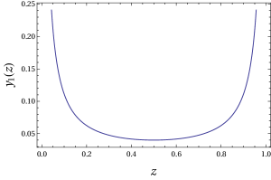
(a)

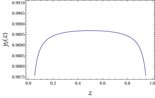
(b)

Figure 4: Behavior of $y_{1}(z)$ and $y_{2}(z)$ as functions of $z$ at $c\,=\,0.01$.

To find the integration limits of $y_{1}$ and $y_{2}$ we proceed as follows. First, going back to eq. (75), the $\delta$-function can be also used to solve for $y$, for which there are two solutions,

$$y_{1}(z) \,=\,\frac{2c}{\left[c^{2}(1-2z)^{2}+2c(z-1)z+(z-1)^{2}z^{2}\right]^{1/2}+c-z^{2}+z}\,,$$ (79)

$$y_{2}(z) \,=\,-\frac{\left[c^{2}(1-2z)^{2}+2c(z-1)z+(z-1)^{2}z^{2}\right]^{1/2}+c-z^{2}+z}{2(c+1)(z-1)z}\,.$$ (80)

Clearly, there are extrema for both expressions at $z=1/2$. The second derivative of $y_{1}(z)$ ($y_{2}(z)$) at $z=1/2$ is positive (negative). Thus the expression of $y_{1}(z)$ in eq. (79) is the lower limit of $y$ and $y_{2}(z)$ in eq. (80) is the upper limit of $y$. Substituting $z=1/2$ in eqs. (79) and (80) we find

$$y_{1}\,=\,\frac{1+4c-\sqrt{1-8c}}{2(1+c)}\,,\qquad y_{2}\,=\,\frac{1+4c+\sqrt{1-8c}}{2(1+c)}\,.$$ (81)

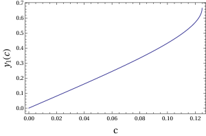
(a)

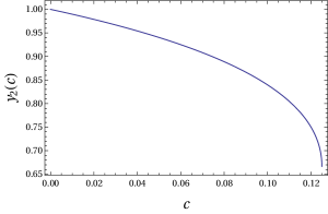
(b)

Figure 5: Lower and upper limits $y_{1}(c)$ and $y_{2}(c)$ respectively as functions of $c$.

The behavior of lower and upper limits are shown in figs. (5a) and (5b). For thrust, the integration limits of the final integration in eq. (17) had simple expressions ($2\tau$ and $1-\tau$ ), and their relation with the respective kinematic configurations were readily visible in fig. (2). To establish the relation between kinematic configurations and the integration limits $y_{1}$ and $y_{2}$ for the case of $c$-parameter, we expand their expressions around $c\,=\,0$ (as $c\to 0$ is the dijet limit),

$$y_{1} \,=\,4c+\mathcal{O}(c^{3}),$$

$$y_{2} \,=\,1-c-3c^{2}+\mathcal{O}(c^{3}).$$ (82)

In the dijet limit, the upper limit of $y$ corresponds to either $(i)$ a back-to-back hard gluon and quark–anti-quark collinear pair $(ii)$ soft quark (or soft anti-quark) emission, or $(iii)$ the hard gluon collinear to the quark or the anti-quark. The lower limit in dijet limit corresponds to a soft gluon emission and a back-to-back quark and anti-quark. Thus these upper and lower limits correspond to different points in the phase space, as expected. The integration over $y$ in eq. (78) produces incomplete elliptic integrals of three types, each with somewhat involved arguments and coefficients. After conversion to their so-called complete counterparts, and carefully collecting their coefficients, the final expression can be organized in a compact form [100] as follows

$$\frac{1}{\sigma_{0}(s)}\frac{d\sigma}{dc}\Bigg{|}_{\text{NLO}}\,=\,\frac{2\alpha_{s}}{3\pi}\bigg{(}e(c)\ {\rm{E}}[m_{1}(c)]+p(c)\ {\Pi}[n_{1}(c),m_{1}(c)]+k(c)\ {\rm{K}}[m_{1}(c)]\bigg{)}\,,$$ (83)

where ${\rm{E}}$, ${\Pi}$, and ${\rm{K}}$ are the complete elliptic integrals of the first, second, and third kind. The integral representation of these elliptic integrals are as following

$${\rm{E}}[m] \,=\,\int^{1}_{0}dt\ \frac{\sqrt{1-m^{2}t^{2}}}{\sqrt{1-t^{2}}}\,,$$

$${\Pi}[n,m] \,=\,\int^{1}_{0}\frac{dt}{(1-nt^{2})\sqrt{(1-t^{2})(1-m^{2}t^{2})}}\,,$$

$${\rm{K}}[m] \,=\,\int^{1}_{0}\frac{dt}{\sqrt{(1-t^{2})(1-m^{2}t^{2})}}\,.$$ (84)

Here $m$, and $n$ are the parameter and characteristic of the elliptic integrals, respectively. The arguments of these elliptic integrals in eq. (83) have the following form

$$n_{1}(c) \,=\,\frac{2\sqrt{1-8c}}{1+\sqrt{1-8c}-4c}\,,$$

$$m_{1}(c) \,=\,\frac{2\sqrt{1-8c}}{1+\sqrt{1-8c}-4c-8c^{2}}\,.$$ (85)

The behavior of these arguments is shown in fig. (6). We computed eq. (83) throughout with a massless on-shell gluon and it agrees with the characteristic function derived in [100] for finite gluon virtuality $\xi$, in the limit $\xi\to 0$.

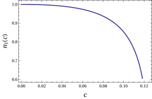
(a)

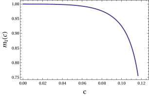
(b)

Figure 6: Behavior of arguments $n_{1}(c)$ and $m_{1}(c)$.

Notice that the arguments have monotonic behavior. The elliptic integrals in eq. (83) have the following asymptotic behavior as $c\to 0$

$${\rm{E}}[m_{1}(c)]\,=\, 1+\mathcal{O}(c^{3}\log{c})\,,$$

$${\rm{\Pi}}[n_{1}(c),m_{1}(c)]\,=\, -\frac{\log{c}}{8c^{2}}-\frac{1+\log{c}}{4c}+\mathcal{O}(c^{0}\log{c})\,,$$ (86)

$${\rm{K}}[m_{1}(c)]\,=\, -\frac{3\log{c}}{2}+\mathcal{O}(c^{3}\log{c})\,.$$

The expressions for the coefficients appearing in eq. (83) are

$$e(c)\,=\, \frac{-3(1+2c)\sqrt{1-4c(1+2c)+\sqrt{1-8c}}}{\sqrt{2}c(1+c)^{3}}\,,$$

$$p(c)\,=\, \frac{\sqrt{2}(2+c+2c^{2})(1-\sqrt{1-8c})^{2}}{c(1+c)^{3}\sqrt{1-4c(1+2c)+\sqrt{1-8c}}}\,,$$ (87)

$$k(c)\,=\, \frac{4\sqrt{2}(1-2c(2+c))}{(1+c)^{3}\sqrt{1-4c(1+2c)+\sqrt{1-8c}}}\,.$$

Their expansions around $c=0$ are

$$e(c)\,=\, -\frac{3}{c}+9+12c+36c^{2}+\mathcal{O}(c^{3})\,,$$

$$p(c)\,=\, 32c+112c^{2}+\mathcal{O}(c^{3})\,,$$ (88)

$$k(c)\,=\, 4-20c+48c^{2}+\mathcal{O}(c^{3})\,.$$

The coefficient $e(c)$, when multiplied by the complete elliptic integral of the second kind $E[m_{1}(c)]$ yields NLL terms at LP, the coefficient $p(c)$, multiplied with the complete elliptic integral of the third kind ${\Pi}[n_{1}(c),m_{1}(c)]$ produces LL and NLL contributions at both LP and NLP, while the coefficient $k(c)$ together with the complete elliptic integral of the first kind $K[m_{1}(c)]$ also produces LL terms at NLP. From eqs. (85), (86) and (88) the $c$-parameter distribution at NLO for small-$c$ reads,

$$\frac{1}{\sigma_{0}(s)}\frac{d\sigma}{dc}\Bigg{|}_{\text{NLO}}\,$$

$$=\,\frac{2\alpha_{s}}{3\pi}\biggl{(}\frac{-3-4\log{c}}{c}+1-28\log{c}+\mathcal{O}(c)\biggr{)}.$$ (89)

We have computed the $c$-parameter distribution here without approximating the event shape variable or the matrix element squared, similar to what we did for thrust in eq. (29). The above result, which agrees with [99, 100], contains the contributions from all regions of the phase space. By comparing eq. (89) and eq. (29) we observe that the LP terms for both event shape variables have an identical structure in the dijet limit. Further similarities between these event-shape variables are discussed in  [107, 108, 109, 110, 111]. The expression eq. (89) does not fully expose the relation to different kinematical configurations. To do so, we list the upper and lower limit contributions of the $y$ integral separately. When computing the contributions from the upper and lower limits separately we have observed that it is only the coefficients $e(c),p(c)\,\text{and}\,k(c)$ of the elliptic integrals that differ, while the general form of the elliptic integrals remains the same as in eq. (83). From the upper limit of eq. (78) we have, for small-$c$,

$$e_{\text{u}}(c) \,=\,-\frac{3}{c}+9+12c+36c^{2}+\mathcal{O}(c^{3})\,,$$

$$p_{\text{u}}(c) \,=\,0\,,$$ (90)

$$k_{\text{u}}(c) \,=\,-12-24c-108c^{2}+\mathcal{O}(c^{3})\,,$$

For the lower limit, the behavior reads

$$e_{\text{l}}(c) \,=\,0\,,$$

$$p_{\text{l}}(c) \,=\,-32c-112c^{2}-912c^{3}+\mathcal{O}(c^{7/2})\,,$$ (91)

$$k_{\text{l}}(c) \,=\,-16-4c-156c^{2}+\mathcal{O}(c^{3})\,.$$

Since $p_{u}(c)\,=\,e_{l}(c)\,=\,0$, no LL terms at LP derive from the upper limit, nor do we find NLL terms at LP from the lower limit. Collecting the upper and lower limit contributions for the $c$-parameter distribution in the dijet limit leads to

$$\frac{1}{\sigma_{0}(s)}\frac{d\sigma}{dc}\Bigg{|}_{\text{u}} \,=\,\ \frac{2\alpha_{s}}{3\pi}\left(-\frac{3}{c}+9(1+2\log c)+\mathcal{O}(c)\right),$$ (92)

$$\frac{1}{\sigma_{0}(s)}\frac{d\sigma}{dc}\Bigg{|}_{\text{l}} \,=\,\ \frac{2\alpha_{s}}{3\pi}\left(\frac{4\log c}{c}+2(4+23\log c)+\mathcal{O}(c)\right).$$ (93)

Thus the upper limit of $y$ in the dijet limit corresponds to various kinematic configurations involving a hard gluon such as hard gluon being back-to-back with quark (anti-quark) and collinear to anti-quark (quark), which produces NLL terms at LP. As discussed the upper limit also corresponds to the soft quark/anti-quark emissions, LL and NLL terms at NLP also arise from this limit. The lower limit of $y$ corresponds to kinematic configurations involving a soft gluon and thus yields LL terms at both LP and NLP. No NLL terms at LP are generated here, although there is a NLL contribution at NLP.

IV.2 Next-to-leading power corrections to $c$-parameter from shifted kinematics

We next compute the $c$-parameter distribution using the shifted kinematics method, and again assess to what extent LP and NLP terms in the exact NLO calculation are reproduced. The approximation is

$$\frac{1}{\sigma_{0}(s)}\frac{d\sigma}{dc}\Bigg{|}_{\text{shift}}\,=\,\frac{1}{2s}\int d\Phi_{3}\ \overline{\sum} |\mathcal{M}_{\text{shift}}(x_{1},x_{2})|^{2}\$$

$$\times\delta\left(c(y,z)-c\right)\,.$$ (94)

The shifted matrix element in eq. (33), when written in terms of the transformed variables ($y,z$), takes the form

$$\overline{\sum} |\mathcal{M}_{\text{shift}}(y,z)|^{2}$$

$$\,=\,8(e^{2}e_{q})^{2}N_{c}C_{F}g_{s}^{2}\frac{1}{3Q^{2}}\left(\frac{2(y-1)}{y^{2}(z-1)z}\right).$$ (95)

Again, we make no approximation to the event shape definition itself. We then proceed in the same manner as with the exact matrix element. We have

$$\frac{1}{\sigma_{0}(s)}\frac{d\sigma}{dc}\Bigg{|}_{\text{shift}} \,=\,\ \frac{2\alpha_{s}}{3\pi}\int^{1}_{0}dy\int^{1}_{0}dz\frac{2(1-y(1-z))^{2}(1-yz)^{2}}{(1-y)^{2}y^{2}z(z-1)(2z-1)}\bigg{(}\delta(z-z_{1})+\delta(z-z_{2})\bigg{)}\,,$$ (96)

where $z_{1}$ and $z_{2}$ are provided in eq. (77). After the $z$ integration we have

$$\frac{1}{\sigma_{0}(s)}\frac{d\sigma}{dc}\Bigg{|}_{\text{shift}}\,=\,\ \frac{2\alpha_{s}}{3\pi}\int^{y_{2}}_{y_{1}}dy\frac{4(y-1)^{2}}{c\sqrt{y\left(y+cy-1\right)\left(c(y-2)^{2}+(y-1)y\right)}}\,.$$ (97)

The result of $y$ integration can again be organized in a manner similar to eq. (83) as

$$\frac{1}{\sigma_{0}(s)}\frac{d\sigma}{dc}\Bigg{|}_{\text{shift}}\,=\,\frac{2\alpha_{s}}{3\pi}\bigg{(}e_{\text{s}}(c)E[m_{1}(c)]+p_{\text{s}}(c)\Pi[n_{1}(c),m_{1}(c)]+k_{\text{s}}(c)K[m_{1}(c)]\bigg{)}\,,$$ (98)

A comparison of eq. (97) with eq. (78) shows a significant simplification of the integrand, where the subscript s on the coefficients on the right indicates the shifted kinematics method. The elliptic integrals and their arguments are given in eqs. (86) and (85) respectively.

The coefficients in eq. (98) do change from the exact result, and we find

$$k_{\text{s}}(c)\,=\, -\frac{\sqrt{2-2\sqrt{1-8c}-8c-16c^{2}}}{c^{3/2}(1+c)^{5/2}}\,,$$

$$e_{\text{s}}(c)\,=\, -\frac{(1+\sqrt{1-8c}-4c)\ \sqrt{1-\sqrt{1-8c}-4c-8c^{2}}}{2\sqrt{2}c^{5/2}(1+c)^{5/2}}\,,$$ (99)

$$p_{\text{s}}(c)\,=\, \frac{(1-\sqrt{1-8c}-4c)\ \sqrt{1-\sqrt{1-8c}-4c-8c^{2}}}{\sqrt{2}c^{5/2}(1+c)^{5/2}}\,.$$

Their small-$c$ behavior is

$$e_{\text{s}}(c)\,=\, -\frac{4}{c}+16-4c+72c^{2}+\mathcal{O}(c^{3})\,,$$

$$p_{\text{s}}(c)\,=\, 32c+128c^{2}+\mathcal{O}(c^{3})\,,$$ (100)

$$k_{\text{s}}(c)\,=\, -8c+\mathcal{O}(c^{3})\,.$$

Expanding around $c=0$, the $c$-parameter distribution from shifted kinematics approximation reads

$$\frac{1}{\sigma_{0}(s)}\frac{d\sigma}{dc}\Bigg{|}_{\text{shift}}\,$$

$$=\,\ \frac{2\alpha_{s}}{3\pi}\bigg{(}\frac{-4-4\log{c}}{c}+8-24\log{c}+\mathcal{O}(c)\bigg{)}.$$ (101)

For better insight, it is again useful to examine separately the contributions of the upper and lower of the $y$ integral. The small-$c$ behavior of the coefficients of the elliptic integrals appearing from the upper limit of eq. (97) is

$$e_{\text{su}}(c) \,=\,-\frac{4}{c}+16-4c+72c^{2}+252c^{3}+\mathcal{O}(c^{7/2}),$$

$$p_{\text{su}}(c) \,=\,0,$$ (102)

$$k_{\text{su}}(c) \,=\,-16-16c-144c^{2}-688c^{3}+\mathcal{O}(c^{7/2})\,.$$

For the lower limit we have

$$e_{\text{sl}}(c) \,=\,0,$$

$$p_{\text{sl}}(c) \,=\,-32c-128c^{2}-928c^{3}+\mathcal{O}(c^{7/2}),$$ (103)

$$k_{\text{sl}}(c) \,=\,-16-8c-144c^{2}-616c^{3}+\mathcal{O}(c^{7/2}).$$

Note that the $\mathcal{O}(c^{3})$ terms contribute at NNLP accuracy. We now have

$$\frac{1}{\sigma_{0}(s)}\frac{d\sigma}{dc}\Bigg{|}_{\text{su}} \,=\,\ \frac{2\alpha_{s}}{3\pi}\left(-\frac{4}{c}+8(2+3\log c)+\mathcal{O}(c)\right),$$ (104)

$$\frac{1}{\sigma_{0}(s)}\frac{d\sigma}{dc}\Bigg{|}_{\text{sl}} \,=\,\ \frac{2\alpha_{s}}{3\pi}\left(\frac{4\log c}{c}+8(1+6\log c)+\mathcal{O}(c)\right).$$ (105)

From the above two expressions, we observe that the lower (upper) limit fully captures the LL (NLL) at LP, while the LL and NLL at NLP receive contributions from both limits. The results for the $c$-parameter distributions at NLO up to NLP, obtained from the exact and shifted kinematics computation, are given in eqs. (89) and (101), respectively. The integrand in the shifted kinematics method was considerably simpler than for the exact computation. At LP, the method reproduced the LL term. The NLL term at LP was not fully reproduced because the contribution from the hard-collinear gluon is absent. Similarly, not all of the LL at NLP is captured, due to the absence of from soft quark and soft anti-quark contributions. Recall that the shifted kinematics method does not account for soft quark contributions, which we computed separately using soft quark emission vertices in section III.2.

We again examine the remaining contributions to the $c$-parameter distribution, such as those from the soft quark, soft anti-quark, and hard-collinear gluon configurations. This allows the mapping of all of the contributions to the $c$-parameter from various regions of the phase space. When expressed in terms of the transformed $(y,z)$ variables the remainder matrix element as described in eq. (49) reads

$$\overline{\sum}|{\mathcal{M}}_{\text{rem}}(y,z)|^{2}\,=\,8 (e^{2}e_{q})^{2}N_{c}C_{F}g_{s}^{2}\frac{1}{3Q^{2}}$$

$$\times\biggl{(}\frac{1}{z}+\frac{1}{1-z}-2\biggr{)}.$$ (106)

The expression for $c$-parameter distribution using the above matrix element squared is

$$\frac{1}{\sigma_{0}(s)}\frac{d\sigma}{dc}\Bigg{|}_{\text{rem}}=\frac{2\alpha_{s}}{3\pi}\int^{1}_{0}dy\int^{1}_{0}dz\frac{1}{z(1-z)}\Big{(}\delta(z-z_{1})+\delta(z-z_{2})\Big{)}\frac{-y(y-1)^{2}\left(1-2z(1-z)\right)}{(cy+y-1)\sqrt{y(cy+y-1)\left(c(y-2)^{2}+(y-1)y\right)}},$$ (107)

with $z_{1}$ and $z_{2}$ are given in eq. (77). After performing the $z$ integration we are left with

$$\frac{1}{\sigma_{0}(s)}\frac{d\sigma}{dc}\Bigg{|}_{\text{rem}}\,=\,\frac{2\alpha_{s}}{3\pi}\int^{y_{1}}_{y_{2}}dy\ \frac{-2y(y-1)(c((y-2)y+2)+(y-1)y)}{c(cy+y-1)\sqrt{y(cy+y-1)\left(c(y-2)^{2}+(y-1)y\right)}}\,.$$ (108)

with $y_{1}$ and $y_{2}$ given in eq. (81). The outcome takes again the form as in eq. (83), somewhat more complicated than either of the two approximations. The result can be written as

$$\frac{1}{\sigma_{0}(s)}\frac{d\sigma}{dc}\Bigg{|}_{\text{rem}}\,=\,\frac{2\alpha_{s}}{3\pi}\bigg{(}e_{\text{r}}(c)\ E[m_{1}(c)]+p_{\text{r}}(c)\ \Pi[n_{1}(c),m_{1}(c)]+k_{\text{r}}(c)\ K[m_{1}(c)]\bigg{)},$$ (109)

The small-$c$ behavior of the coefficients reads

$$e_{r}(c) \,=\,\frac{1}{c}-7+16c-36c^{2}+9c^{3}+\mathcal{O}(c^{7/2})\,,$$

$$p_{r}(c) \,=\,-16c-16c^{3}+\mathcal{O}(c^{7/2})\,,$$ (110)

$$k_{r}(c) \,=\,4-12c+48c^{2}+16c^{3}+\mathcal{O}(c^{7/2})\,,$$

$$\frac{1}{\sigma_{0}(s)}\frac{d\sigma}{dc}\Bigg{|}_{\text{rem}}\,=\,\frac{2\alpha_{s}}{3\pi}\left(\frac{1}{c}-7-4\log c+\mathcal{O}(c)\right)\,.$$ (111)

Here we indeed see contributions from the hard-collinear gluon, the soft quark, and anti-quark configurations, which yield NLL terms at LP (hard-collinear gluon) as well as LL terms at NLP (soft quark/anti-quark) respectively. Combining these contributions with the outcome of shifted kinematics approximation eq. (101) allows us to fully map the distributions of the $c$-parameter to the different kinematical configurations.

Let us finally break the contributions from remaining term also down into upper and lower limit components. The coefficients from the upper limit of eq. (108) yield

$$e_{\text{ru}}(c) \,=\,\frac{1}{c}-7+16c-36c^{2}+9c^{3}+\mathcal{O}(c^{7/2})\,,$$

$$p_{\text{ru}}(c) \,=\,0\,,$$ (112)

$$k_{\text{ru}}(c) \,=\,4-8c+36c^{2}+64c^{3}+\mathcal{O}(c^{7/2})\,.$$

while for the lower limit, we have

$$e_{\text{rl}}(c) \,=\,0,$$

$$p_{\text{rl}}(c) \,=\,16c+16c^{3}+\mathcal{O}(c^{7/2}),$$ (113)

$$k_{\text{rl}}(c) \,=\,4c-12c^{2}+48c^{3}+\mathcal{O}(c^{7/2}).$$

Using eqs. (85), (86) and above two expressions, the contributions to the $c$-parameter distribution from the upper and lower limit respectively are

$$\frac{1}{\sigma_{0}(s)}\frac{d\sigma}{dc}\Bigg{|}_{\text{ru}} \,=\,\ \frac{2\alpha_{s}}{3\pi}\left(\frac{1}{c}-7-6\log c+\mathcal{O}(c)\right),$$ (114)

$$\frac{1}{\sigma_{0}(s)}\frac{d\sigma}{dc}\Bigg{|}_{\text{rl}} \,=\,\ \frac{2\alpha_{s}}{3\pi}\bigg{(}-2\log c+\mathcal{O}(c)\bigg{)}.$$ (115)

The missing LL terms at NLP have been generated here. The upper limit contributes to the missing NLL term at LP (related to hard-collinear gluon emission) and NLP. Both limits contain LL terms at NLP (soft (anti-)quark emission).

IV.3 Numerical assessment of the shifted kinematics approximations for $c$-parameter

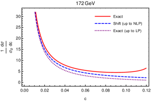
(a)

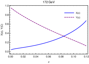
(b)

Figure 7: In (a), we plot comparison of the $c$-parameter distribution. We show the exact result (solid red curve) in eq. (83), the shifted approximation (dashed blue curve) up to NLP terms given in eq. (101). We also plot the exact LP term given in eq. (89) (dotted purple curve). In (b), we show behavior of $X(c)$ (solid blue curve) and $Y(c)$ (purple dashed curve) from eqs. (116) and (117) respectively vs. $c$.

We analyze our $c$-parameter results numerically. In the small-$c$ limit, the effectiveness of the shifted kinematics method is evident from fig. (7a), the shifted kinematics result provides a better approximation to the exact result, than the exact result taken up to LP terms only, even though we did not generate all the dominant terms at LP and NLP from this approximation. The $c$-parameter distribution in fig. (7a) has a more pronounced departure of the LP terms from the exact result than the thrust distribution in fig. (3a). This is due to the $c$-parameter distribution having a larger LL coefficient at NLP than thrust. We define $X(c)$ and $Y(c)$ in similar fashion to $X(\tau)$ and $Y(\tau)$ in eqs. (65) and (66) as

$$X(c) \,=\,\frac{\frac{1}{\sigma_{0}(s)}\frac{d\sigma}{dc}\Big{|}_{\text{NLO}}-\frac{1}{\sigma_{0}(s)}\frac{d\sigma}{dc}\Big{|}_{\text{shift-NLP}}}{\frac{1}{\sigma_{0}(s)}\frac{d\sigma}{dc}\Big{|}_{\text{NLO}}},$$ (116)

$$Y(c) \,=\,\frac{\frac{1}{\sigma_{0}(s)}\frac{d\sigma}{dc}\Big{|}_{\text{NLO-LP}}}{\frac{1}{\sigma_{0}(s)}\frac{d\sigma}{dc}\Big{|}_{\text{NLO}}}\,,$$ (117)

and exhibit them in fig. (7b). $X(c)$ exhibits similar behavior as the analogous case for thrust in fig. (3b), but the deviation of $X(c)$ from zero is faster with increasing $c$. $Y(c)$ decreases sharply from unity as $c$ increases, a behavior opposite to thrust in fig. (7b). Indeed, due to the large negative LL coefficient at NLP for the $c$-parameter, the denominator here increases sharply. More precisely, for the $c$-parameter, the LL coefficient at NLP is seven times that at LP, with the same sign, while for thrust, the LL coefficient at NLP is half that of LP, with the opposite sign.

V Conclusions

The fixed order results in perturbation theory for massless fields contain logarithms of the (small) ratio of energy scales, arising from soft or collinear radiation. They occur at both leading and next-to-leading power of this ratio. This work focuses on NLP terms appearing in the thrust and $C$-parameter event shape distribution. We identify in exact NLO results the origin of large logarithmic terms at LP and NLP. Subsequently we provide an approximation of these results using the recent shifted kinematics method, designed to capture large logarithms at NLP accuracy due to soft gluon emission. Moreover we compute soft quark emission contributions using corresponding effective Feynman rules.

This formalism indeed reproduces the dominant contributions at LP and NLP from soft gluon radiation correctly for both thrust and $c$-parameter. The remaining LL terms at NLP are reproduced the soft (anti-)quark emission, as anticipated in [46, 112]. We were able to map the various sources of contributions at LP and NLP, using an integral form, and its limits, for the distributions.

Our detailed diagnosis of NLP terms in event shape variables, and demonstration that they can be fully reproduced using a shifted kinematics approach together with soft fermion emission vertices, should be a useful resource towards further understanding of NLP terms, in particular those arising from final state emissions.

Appendix A Transformation of incomplete elliptic integrals

In this appendix, we demonstrate how we handle the incomplete elliptic integrals that appear in the expression of $c$-parameter distribution. The final expression for the $c$-parameter distribution is written in a compact manner in eq. (83), where $K$, $E$ and $\Pi$ are the complete elliptic integrals of the first, second and third kind, respectively. However, when we perform the integration over final variable $y$ in eqs. (78), (97) and (108), this integration produces incomplete elliptic integrals $F$, $E$, and $\Pi$. These incomplete elliptic integrals are later converted into complete integrals to arrive at eq. (83), as first written in [100]. The three kinds of incomplete elliptic integrals appearing in $c$-parameter distribution are

$$F[\phi,m]\,\equiv\, \int_{0}^{\phi}d\theta\frac{1}{\sqrt{1-m\sin^{2}\theta}}$$

$$\,=\, \int_{0}^{\sin\phi}\frac{dt}{\sqrt{(1-t^{2})(1-mt^{2})}}\,,$$ (118)

$$E[\phi,m]\,\equiv\, \int_{0}^{\phi}d\theta\sqrt{1-m\sin^{2}\theta}\,$$

$$\,=\, \,\int_{0}^{\sin\phi}dt\sqrt{\frac{1-mt^{2}}{1-t^{2}}}\,,$$ (119)

$$\hskip 19.91684pt\Pi[n,\phi,m]\,\equiv\, \int_{0}^{\phi}d\theta\frac{1}{(1-m\sin^{2}\theta)\sqrt{1-m\sin^{2}\theta}}$$

$$\,=\, \int_{0}^{\sin\phi}\frac{dt}{(1-nt^{2})\sqrt{(1-t^{2})(1-mt^{2})}}\,.$$ (120)

Here $\phi,m$, and $n$ are called the amplitude, parameter, and characteristic of the elliptic integrals, respectively. Eq. (IV.1) gives their respective complete form. The corresponding transformation into a complete elliptic integral can be performed using the rule

$$F[\phi,m] \,=\,K[m],$$

$$E[\phi,m] \,=\,E[m],$$ (121)

$$\Pi[n,\phi,m] \,=\,\Pi[n,m].$$

The above transformation is only possible when the amplitude $\phi=\pi/2$. The indefinite integration of eqs. (78), (97) and (108) results in multiple incomplete elliptic integrals with only two unique amplitudes in their arguments, namely $\phi_{1}(c,y)$ and $\phi_{2}(c,y)$, given by

$$\phi_{1}(c,y) \,=\,\left(\frac{-1+\sqrt{1-8c}-4c+8c/y}{2\sqrt{1-8c}}\right)^{1/2},$$ (122)

$$\phi_{2}(c,y) \,=\,\left(\frac{1+\sqrt{1-8c}+4c-8c/y}{2\sqrt{1-8c}}\right)^{1/2}.$$ (123)

The amplitudes $\phi_{1}(c,y)$ and $\phi_{2}(c,y)$ are present in the arguments of all three kinds of incomplete elliptic integrals. If we directly substitute the upper limit ($y_{2}$) after integration, then none of the incomplete elliptic integrals with the amplitude $\phi_{1}(c,y)$ can be reduced into complete elliptic integral since

$$\phi_{1}(c,y)\Big{|}_{y\,=\,y_{2}}\,=\,0.$$ (124)

The transformation into complete elliptic integrals holds only when $\phi_{1}=\pi/2$ as given in eq. (A). However, the incomplete elliptic integrals with the amplitude $\phi_{2}(c,y)$ upon substitution of upper limit can be directly reduced into complete elliptic integral as

$$\phi_{2}(c,y)\Big{|}_{y\,=\,y_{2}}\,=\,\frac{\pi}{2}.$$ (125)

We observe a similar but opposite behavior when we substitute the lower limit ($y_{1}$) into the integration result, this time, the incomplete elliptic integrals with the amplitude $\phi_{1}(c,y)$ can be reduced into complete elliptic integral as

$$\phi_{1}(c,y)\Big{|}_{y\,=\,y_{1}}\,=\,\frac{\pi}{2},$$ (126)

while the elliptic integrals with amplitude $\phi_{2}(c,y)$ cannot be reduced into complete elliptic integral as

$$\phi_{2}(c,y)\Big{|}_{y\,=\,y_{1}}\,=\,0.$$ (127)

In order to resolve the issue of transforming the incomplete elliptic integrals into complete elliptic integrals, we modify the upper and lower limits of $y$ integration as

$$(y_{1},y_{2})\to(y_{1}+e,y_{2}+e)\,,$$ (128)

where $e$ is an infinitesimal real off-set parameter that will be taken to zero at the end. The relative sign of $e$ does not affect the final expression for $c$-parameter distribution, which is independent of this parameter $e$. When we substitute the upper limit of integration $y_{2}$ with the off-set parameter as defined in the above expression, the amplitudes $\phi_{1}(c,y)$ and $\phi_{2}(c,y)$ modify and have the following form

$$\phi_{1}(c,y,e)\Big{|}_{y\,=\,y_{2}+e} \,=\,\left(\frac{\left(-4c+\sqrt{1-8c}-1\right)(c+1)e}{\sqrt{1-8c}\left(2c(e+2)+\sqrt{1-8c}+2e+1\right)}\right)^{1/2}\,,$$ (129)

$$\phi_{2}(c,y,e)\Big{|}_{y\,=\,y_{2}+e} \,=\,\left(\frac{-\frac{16(c+1)c}{2c(e+2)+\sqrt{1-8c}+2e+1}+4c+\sqrt{1-8c}+1}{2\sqrt{1-8c}}\right)^{1/2},$$ (130)

similarly, from the lower limit, the amplitudes are

$$\phi_{1}(c,y,e)\Big{|}_{y\,=\,y_{1}+e} \,=\,\left(\frac{\frac{16(c+1)c}{2c(e+2)-\sqrt{1-8c}+2e+1}-4c+\sqrt{1-8c}-1}{2\sqrt{1-8c}}\right)^{1/2}\,,$$ (131)

$$\phi_{2}(c,y,e)\Big{|}_{y\,=\,y_{1}+e} \,=\,\left(-\frac{(c+1)\left(4c+\sqrt{1-8c}+1\right)e}{\sqrt{1-8c}\left(-2c(e+2)+\sqrt{1-8c}-2e-1\right)}\right)^{1/2}.$$ (132)

Note that, it is necessary to use this parameter because the straightforward substitution of limits did not allow the transformation of every incomplete elliptic integral. Let us consider a few examples to demonstrate how this off-set parameter solves the problem with incomplete elliptic integrals that cannot be reduced into complete elliptic integrals as their amplitude $\phi\neq\pi/2$. We can categorize all the elliptic integrals appearing after $y$ integration into two classes according to their amplitudes $\phi$ as $(i)$ non-reducible incomplete elliptic integrals $(\phi\neq\pi/2)$, and $(ii)$ reducible incomplete elliptic integrals $(\phi=\pi/2)$.

A.1 Non-reducible incomplete elliptic integrals

Here we consider an incomplete elliptic integral that appears from the upper limit contributions, the expression of the elliptic integral is

$$E[\phi_{1}(c,e),m_{1}(c)]\,=\,E\left[\sin^{-1}\left(\frac{\left(-4c+\sqrt{1-8c}-1\right)(c+1)e}{\sqrt{1-8c}\left(2c(e+2)+\sqrt{1-8c}+2e+1\right)}\right)^{1/2},\ \frac{2\sqrt{1-8c}}{1+\sqrt{1-8c}-4c-8c^{2}}\right]\,,$$ (133)

where $m_{1}$ is given in eq. (85), the amplitude of this elliptic function is

$$\phi_{1}(c,e)\,=\,\sin^{-1}\left(\frac{\left(-4c+\sqrt{1-8c}-1\right)(c+1)e}{\sqrt{1-8c}\left(2c(e+2)+\sqrt{1-8c}+2e+1\right)}\right)^{1/2}.$$ (134)

The elliptic integral in eq. (133) cannot be reduced into a complete elliptic integral as in the limit $e\to 0$ the amplitude $\phi_{1}(c,e)\to 0$. However, we can expand this elliptic integral in powers of $e$ around $e=0$, upon expanding we get

$$E[\phi_{1}(c,e),m_{1}(c)] \,=\,\sqrt{\frac{\left(-4c+\sqrt{1-8c}-1\right)(c+1)}{\sqrt{1-8c}\left(4c+\sqrt{1-8c}+1\right)}}\sqrt{e}+\mathcal{O}(e^{3/2})$$ (135)

The expansion’s first term, proportional to $e^{1/2}$, is the only significant term in the limit when $e\to 0$. The next term in the above expression is proportional to $e^{3/2}$, and can be dropped. The small-$e$ expression for these specific incomplete elliptic integrals occurring is then stored in the form

$$E[\phi_{1}(c,e),m_{1}(c)]\,=\,\sqrt{\frac{\left(-4c+\sqrt{1-8c}-1\right)(c+1)}{\sqrt{1-8c}\left(4c+\sqrt{1-8c}+1\right)}}\sqrt{e}.$$ (136)

Now, we shift our attention toward the elliptic integrals that appears from the lower limit contribution, one such incomplete elliptic integral is

$$F[\phi_{2}(c,e),m_{1}(c)]\,=\,F\left[\sin^{-1}\left(\frac{(c+1)\left(4c+\sqrt{1-8c}+1\right)e}{\sqrt{1-8c}\left(2c(e-2)+\sqrt{1-8c}+2e-1\right)}\right)^{1/2},\ \frac{2\sqrt{1-8c}}{1+\sqrt{1-8c}-4c-8c^{2}}\right]\,.$$ (137)

The above elliptic integral cannot be reduced into a complete elliptic integral as the amplitude $\phi_{2}(c,e)$ is

$$\phi_{2}(c,e)\,=\,\sin^{-1}\left(\frac{(c+1)\left(4c+\sqrt{1-8c}+1\right)e}{\sqrt{1-8c}\left(2c(e-2)+\sqrt{1-8c}+2e-1\right)}\right)^{1/2}$$ (138)

and in the limit $e\to 0$ the amplitude $\phi_{2}(c,e)\to 0$. Following the similar procedure as in eq. (136), the elliptic integral in eq. (137) is expanded around $e=0$, we get

$$F[\phi_{2}(c,e),m_{1}(c)]=\sqrt{\frac{(c+1)\left(4c+\sqrt{1-8c}+1\right)}{\sqrt{1-8c}\left(-4c+\sqrt{1-8c}-1\right)}}\sqrt{e}\,.$$ (139)

The coefficients of these elliptic functions depend on $e$ when the integration limits are modified in accordance with eq. (128). When we expand our final result in powers of $e$, the negative powers of $\sqrt{e}$ from the coefficients combine with the positive powers of $\sqrt{e}$ from the stored expressions of non-reducible incomplete elliptic integrals to yield few terms independent of $e$. Subsequently $e$ can be set to zero.

Observable	Matrix element	Distribution up to NLP
Thrust	Exact	$$\frac{-3-4\log{\tau}}{\tau}-2+2\log{\tau}$$
Thrust	Shift	$$\frac{-4-4\log{\tau}}{\tau}+4+4\log{\tau}$$
Thrust	Remainder	$$\frac{1}{\tau}-6-2\log{\tau}$$
Thrust	Eikonal	$$\frac{-4\log{\tau}}{\tau}-8-4\log{\tau}$$
c-parameter	Exact	$$\frac{-3-4\log{c}}{c}+1-28\log{c}$$
c -parameter	Shift	$$\frac{-4-4\log{c}}{c}+8-24\log{c}$$
c -parameter	Remainder	$$\frac{1}{c}-7-4\log{c}$$
c -parameter	Eikonal	$$\frac{-4\log{c}}{c}-8-40\log c$$

Table 1: Table for the result of thrust and $c$-parameter distributions calculated using the exact definition of event shape variables and four different definitions of matrix elements.

A.2 Reducible incomplete elliptic integrals

The category of incomplete elliptic integrals, which can be reduced into complete elliptic integrals is easier to handle as compared with non-reducible ones. An elliptic integral appearing from the upper limit contribution is

$$E[\phi_{2}(c,e),m_{1}(c)]\,=\,E\left[\sin^{-1}\left(\frac{-\frac{16(c+1)c}{2c(e+2)+\sqrt{1-8c}+2e+1}+4c+\sqrt{1-8c}+1}{2\sqrt{1-8c}}\right)^{1/2},\ \frac{2\sqrt{1-8c}}{1+\sqrt{1-8c}-4c-8c^{2}}\right]\,,$$ (140)

where the amplitude $\phi_{2}(c,e)$ reads

$$\phi_{2}(c,e)\,=\,\sin^{-1}\left(\frac{-\frac{16(c+1)c}{2c(e+2)+\sqrt{1-8c}+2e+1}+4c+\sqrt{1-8c}+1}{2\sqrt{1-8c}}\right)^{1/2}\,.$$ (141)

In the limit $e\to 0$ the amplitude $\phi_{2}(c,e)\to\pi/2$ and this incomplete elliptic integral can be reduced directly to a complete elliptic integral using reduction formula in eq. (A)

$$E[\phi_{2}(c,e),m_{1}(c)]\,=\,E[m_{1}(c)]\,.$$ (142)

In this way all reducible incomplete elliptic integrals can be substituted with their corresponding complete elliptic integrals. Upon substituting all the complete elliptic integrals and the stored expressions of incomplete elliptic integrals, our final result is expanded in powers of $e$. No negative powers occur, and $e$ can be taken to zero, yielding eq. (83).

Appendix B Eikonal approximation and result summary

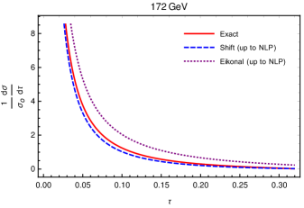
(a)

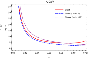
(b)

Figure 8: In (a) and (b), we plot the thrust and $c$-parameter distributions, respectively. We show the exact result (solid red curves) given in eqs. (28) and  (83), the shifted approximation result (dashed blue curves) up to NLP terms given in eqs. (47) and (101) for $\tau$ and $c$ respectively. We also plot the LP term (dotted purple curves) given in eqs. (144) and (145)

B.1 Eikonal approximation to thrust and $c$-parameter distribution

In sections III.3 and IV.3, we compared the shifted approximation with the LP expression of the exact distribution in figs. (3a) and (7a), for the thrust and $c$-parameter distribution, respectively. Here we add the results from the simpler eikonal approximation to the comparison. The eikonal case follows from the approximated matrix element squared

$$\overline{\sum}|\mathcal{M}_{\text{eik}}(x_{1},x_{2})|^{2}\,=\, 8(e^{2}e_{q})^{2}g_{s}^{2}C_{F}N_{c}\frac{1}{3Q^{2}}$$

$$\times\left(\frac{2}{(1-x_{1})(1-x_{2})}\right)\,.$$ (143)

Using the above expression and the exact definitions of thrust and $c$-parameter in eqs. (10) and (69), one finds for their respective distributions

$$\frac{1}{\sigma_{0}(s)}\frac{d\sigma}{d\tau}\Bigg{|}_{\text{NLO}} \,=\,\frac{2\alpha_{s}}{3\pi}\left(\frac{-4\log{\tau}}{\tau}-8-4\log{\tau}+\mathcal{O}(\tau)\right),$$ (144)

$$\frac{1}{\sigma_{0}(s)}\frac{d\sigma}{dc}\Bigg{|}_{\text{NLO}} \,=\,\frac{2\alpha_{s}}{3\pi}\left(\frac{-4\log{c}}{c}-8-40\log{c}+\mathcal{O}(c)\right).$$ (145)

The eikonal matrix element squared generates LL terms at LP correctly, together with some LL and NLL at NLP. It does not capture any NLL term at LP since it lacks contributions from hard-collinear gluon emission. In figs. (8a) and (8b), we plot these eikonal results together with the thrust and c-parameter distributions computed from the exact approach as given in eq. (28) and eq. (83) along with the shifted approximation results up to NLP from eqs. (47) and (101). Clearly for both event shapes the shifted kinematics methods provides a significantly better approximation than the eikonal approximation.

B.2 Table of results

In table 1, we summarize our results for thrust and the $c$-parameter using the different approximations of the matrix elements squared: eikonal, exact, shifted kinematics, as well as the remainder/soft quark part.

References

- Kinoshita and Ukawa [1975] T. Kinoshita and A. Ukawa, Lect. Notes Phys. 39, 55 (1975).
- Lee and Nauenberg [1964] T. D. Lee and M. Nauenberg, Phys. Rev. 133, B1549 (1964).
- Parisi [1980] G. Parisi, Phys. Lett. B 90, 295 (1980).
- Curci and Greco [1980] G. Curci and M. Greco, Phys. Lett. B 92, 175 (1980).
- Sterman [1987] G. Sterman, Nuclear Physics B 281, 310 (1987).
- Catani and Trentadue [1989] S. Catani and L. Trentadue, Nucl. Phys. B 327, 323 (1989).
- Catani and Trentadue [1991] S. Catani and L. Trentadue, Nucl. Phys. B 353, 183 (1991).
- Gatheral [1983] J. G. M. Gatheral, Phys. Lett. B 133, 90 (1983).
- Frenkel and Taylor [1984] J. Frenkel and J. C. Taylor, Nucl. Phys. B 246, 231 (1984).
- Sterman [1981] G. F. Sterman, AIP Conf. Proc. 74, 22 (1981).
- Korchemsky and Marchesini [1993a] G. P. Korchemsky and G. Marchesini, Nucl. Phys. B 406, 225 (1993a), arXiv:hep-ph/9210281 .
- Korchemsky and Marchesini [1993b] G. P. Korchemsky and G. Marchesini, Phys. Lett. B 313, 433 (1993b).
- Forte and Ridolfi [2003] S. Forte and G. Ridolfi, Nucl. Phys. B 650, 229 (2003), arXiv:hep-ph/0209154 .
- Contopanagos et al. [1997] H. Contopanagos, E. Laenen, and G. F. Sterman, Nucl. Phys. B 484, 303 (1997), arXiv:hep-ph/9604313 .
- Becher and Neubert [2006] T. Becher and M. Neubert, Phys. Rev. Lett. 97, 082001 (2006), arXiv:hep-ph/0605050 .
- Schwartz [2008] M. D. Schwartz, Phys.Rev. D77, 014026 (2008).
- Bauer et al. [2008] C. W. Bauer, S. Fleming, C. Lee, and G. Sterman, Phys. Rev. D 78, 034027 (2008).
- Chiu et al. [2009] J.-y. Chiu, A. Fuhrer, R. Kelley, and A. V. Manohar, Phys. Rev. D 80, 094013 (2009).
- Gardi [2002] E. Gardi, Nucl. Phys. B 622, 365 (2002), arXiv:hep-ph/0108222 .
- Agarwal et al. [2021] N. Agarwal, A. Mukhopadhyay, S. Pal, and A. Tripathi, JHEP 03, 155, arXiv:2012.06842 [hep-ph] .
- Laenen [2004] E. Laenen, Pramana 63, 1225 (2004).
- Luisoni and Marzani [2015] G. Luisoni and S. Marzani, Journal of Physics G: Nuclear and Particle Physics 42, 103101 (2015).
- Becher et al. [2015] T. Becher, A. Broggio, and A. Ferroglia, Introduction to Soft-Collinear Effective Theory, Vol. 896 (Springer, 2015) arXiv:1410.1892 [hep-ph] .
- Campbell et al. [2017] J. Campbell, J. Huston, and F. Krauss, The Black Book of Quantum Chromodynamics: A Primer for the LHC Era (Oxford University Press, 2017).
- Agarwal et al. [2023] N. Agarwal, L. Magnea, C. Signorile-Signorile, and A. Tripathi, Phys. Rept. 994, 1 (2023), arXiv:2112.07099 [hep-ph] .
- Bauer et al. [2000] C. W. Bauer, S. Fleming, and M. E. Luke, Phys. Rev. D 63, 014006 (2000), arXiv:hep-ph/0005275 .
- Bauer and Stewart [2001] C. W. Bauer and I. W. Stewart, Phys. Lett. B 516, 134 (2001), arXiv:hep-ph/0107001 .
- Bauer et al. [2001] C. W. Bauer, S. Fleming, D. Pirjol, and I. W. Stewart, Phys. Rev. D 63, 114020 (2001), arXiv:hep-ph/0011336 .
- Bauer et al. [2002] C. W. Bauer, D. Pirjol, and I. W. Stewart, Phys. Rev. D 65, 054022 (2002), arXiv:hep-ph/0109045 .
- Bonocore et al. [2015] D. Bonocore, E. Laenen, L. Magnea, S. Melville, L. Vernazza, and C. D. White, Journal of High Energy Physics 2015, 8 (2015).
- Bonocore et al. [2016] D. Bonocore, E. Laenen, L. Magnea, L. Vernazza, and C. D. White, Journal of High Energy Physics 2016, 121 (2016).
- Moult et al. [2018] I. Moult, I. W. Stewart, G. Vita, and H. X. Zhu, JHEP 08, 013, arXiv:1804.04665 [hep-ph] .
- Beneke et al. [2020a] M. Beneke, A. Broggio, S. Jaskiewicz, and L. Vernazza, JHEP 07, 078, arXiv:1912.01585 [hep-ph] .
- Moult et al. [2019] I. Moult, I. W. Stewart, and G. Vita, JHEP 11, 153, arXiv:1905.07411 [hep-ph] .
- Bahjat-Abbas et al. [2019] N. Bahjat-Abbas, D. Bonocore, J. Sinninghe Damsté, E. Laenen, L. Magnea, L. Vernazza, and C. D. White, JHEP 11, 002, arXiv:1905.13710 [hep-ph] .
- Beneke et al. [2020b] M. Beneke, M. Garny, S. Jaskiewicz, R. Szafron, L. Vernazza, and J. Wang, JHEP 01, 094, arXiv:1910.12685 [hep-ph] .
- Moult et al. [2020a] I. Moult, G. Vita, and K. Yan, JHEP 07, 005, arXiv:1912.02188 [hep-ph] .
- Ajjath et al. [2021] A. H. Ajjath, P. Mukherjee, V. Ravindran, A. Sankar, and S. Tiwari, JHEP 04, 131, arXiv:2007.12214 [hep-ph] .
- Beneke et al. [2020c] M. Beneke, M. Garny, S. Jaskiewicz, R. Szafron, L. Vernazza, and J. Wang, JHEP 10, 196, arXiv:2008.04943 [hep-ph] .
- Ajjath et al. [2022a] A. H. Ajjath, P. Mukherjee, and V. Ravindran, Phys. Rev. D 105, 094035 (2022a), arXiv:2006.06726 [hep-ph] .
- van Beekveld et al. [2021a] M. van Beekveld, L. Vernazza, and C. D. White, JHEP 12, 087, arXiv:2109.09752 [hep-ph] .
- Liu and Neubert [2020a] Z. L. Liu and M. Neubert, JHEP 04, 033, arXiv:1912.08818 [hep-ph] .
- Krämer et al. [1998] M. Krämer, E. Laenen, and M. Spira, Nuclear Physics B 511, 523 (1998).
- Ball et al. [2013] R. D. Ball, M. Bonvini, S. Forte, S. Marzani, and G. Ridolfi, Nuclear Physics B 874, 746 (2013).
- Anastasiou et al. [2015] C. Anastasiou, C. Duhr, F. Dulat, F. Herzog, and B. Mistlberger, Phys. Rev. Lett. 114, 212001 (2015).
- van Beekveld et al. [2020] M. van Beekveld, W. Beenakker, E. Laenen, and C. D. White, JHEP 03, 106, arXiv:1905.08741 [hep-ph] .
- van Beekveld et al. [2021b] M. van Beekveld, E. Laenen, J. Sinninghe Damsté, and L. Vernazza, JHEP 05, 114, arXiv:2101.07270 [hep-ph] .
- Ajjath et al. [2022b] A. H. Ajjath, P. Mukherjee, V. Ravindran, A. Sankar, and S. Tiwari, European Physical Journal C 82, 234 (2022b).
- Laenen et al. [2009] E. Laenen, G. Stavenga, and C. D. White, Journal of High Energy Physics 2009, 054 (2009).
- Laenen et al. [2011] E. Laenen, L. Magnea, G. Stavenga, and C. D. White, Journal of High Energy Physics 2011, 141 (2011).
- Soar et al. [2010] G. Soar, A. Vogt, S. Moch, and J. A. M. Vermaseren, Nuclear Physics 832, 152 (2010).
- de Florian et al. [2014] D. de Florian, J. Mazzitelli, S. Moch, and A. Vogt, Journal of High Energy Physics 2014, 1 (2014).
- Presti et al. [2014] N. A. L. Presti, A. A. Almasy, and A. Vogt, Physics Letters B 737, 120 (2014).
- Bonocore [2020] D. Bonocore, arXiv: High Energy Physics - Theory (2020).
- Gervais [2017a] H. Gervais, Phys. Rev. D 95, 125009 (2017a).
- Gervais [2017b] H. Gervais, Phys. Rev. D 96, 065007 (2017b).
- Gervais [2017c] H. P. Gervais (2017).
- Laenen et al. [2021] E. Laenen, J. Sinninghe Damsté, L. Vernazza, W. Waalewijn, and L. Zoppi, Phys. Rev. D 103, 034022 (2021).
- Beneke et al. [2022] M. Beneke, M. Garny, S. Jaskiewicz, J. Strohm, R. Szafron, L. Vernazza, and J. Wang, JHEP 07, 144, arXiv:2205.04479 [hep-ph] .
- Kolodrubetz et al. [2016] D. W. Kolodrubetz, I. Moult, and I. W. Stewart, JHEP 05, 139, arXiv:1601.02607 [hep-ph] .
- Moult et al. [2017a] I. Moult, L. Rothen, I. W. Stewart, F. J. Tackmann, and H. X. Zhu, Phys. Rev. D 95, 074023 (2017a), arXiv:1612.00450 [hep-ph] .
- Feige et al. [2017] I. Feige, D. W. Kolodrubetz, I. Moult, and I. W. Stewart, JHEP 11, 142, arXiv:1703.03411 [hep-ph] .
- Beneke et al. [2018a] M. Beneke, M. Garny, R. Szafron, and J. Wang, JHEP 03, 001, arXiv:1712.04416 [hep-ph] .
- Beneke et al. [2018b] M. Beneke, M. Garny, R. Szafron, and J. Wang, JHEP 11, 112, arXiv:1808.04742 [hep-ph] .
- Bhattacharya et al. [2019] A. Bhattacharya, I. Moult, I. W. Stewart, and G. Vita, JHEP 05, 192, arXiv:1812.06950 [hep-ph] .
- Beneke et al. [2019a] M. Beneke, M. Garny, R. Szafron, and J. Wang, JHEP 09, 101, arXiv:1907.05463 [hep-ph] .
- Bodwin et al. [2021] G. T. Bodwin, J.-H. Ee, J. Lee, and X.-P. Wang, Phys. Rev. D 104, 116025 (2021), arXiv:2107.07941 [hep-ph] .
- Liu et al. [2021] Z. L. Liu, B. Mecaj, M. Neubert, and X. Wang, Phys. Rev. D 104, 014004 (2021), arXiv:2009.04456 [hep-ph] .
- Boughezal et al. [2017] R. Boughezal, X. Liu, and F. Petriello, JHEP 03, 160, arXiv:1612.02911 [hep-ph] .
- Moult et al. [2017b] I. Moult, I. W. Stewart, and G. Vita, JHEP 07, 067, arXiv:1703.03408 [hep-ph] .
- Chang et al. [2018] C.-H. Chang, I. W. Stewart, and G. Vita, JHEP 04, 041, arXiv:1712.04343 [hep-ph] .
- Beneke et al. [2019b] M. Beneke, A. Broggio, M. Garny, S. Jaskiewicz, R. Szafron, L. Vernazza, and J. Wang, JHEP 03, 043, arXiv:1809.10631 [hep-ph] .
- Ebert et al. [2019] M. A. Ebert, I. Moult, I. W. Stewart, F. J. Tackmann, G. Vita, and H. X. Zhu, JHEP 04, 123, arXiv:1812.08189 [hep-ph] .
- Moult et al. [2020b] I. Moult, I. W. Stewart, G. Vita, and H. X. Zhu, JHEP 05, 089, arXiv:1910.14038 [hep-ph] .
- Liu and Neubert [2020b] Z. L. Liu and M. Neubert, JHEP 06, 060, arXiv:2003.03393 [hep-ph] .
- Liu et al. [2020] Z. L. Liu, B. Mecaj, M. Neubert, X. Wang, and S. Fleming, JHEP 07, 104, arXiv:2005.03013 [hep-ph] .
- Wang [2019] J. Wang, (2019), arXiv:1912.09920 [hep-ph] .
- Banfi et al. [2002] A. Banfi, G. Salam, and G. Zanderighi, JHEP 0201, 018, arXiv:hep-ph/0112156 [hep-ph] .
- Catani et al. [1992] S. Catani, G. Turnock, and B. Webber, Phys. Lett. B 295, 269 (1992).
- Catani et al. [1993] S. Catani, L. Trentadue, G. Turnock, and B. Webber, Nucl.Phys. B407, 3 (1993).
- Ellis et al. [2011] R. Ellis, W. Stirling, and B. Webber, QCD and collider physics, Vol. 8 (Cambridge University Press, 2011).
- Dokshitzer et al. [1998] Y. L. Dokshitzer, A. Lucenti, G. Marchesini, and G. P. Salam, Journal of High Energy Physics 1998, 011 (1998).
- Dasgupta and Salam [2002] M. Dasgupta and G. P. Salam, Journal of High Energy Physics 2002, 017 (2002).
- Antonelli et al. [2000] V. Antonelli, M. Dasgupta, and G. P. Salam, Journal of High Energy Physics 2000, 001 (2000).
- Ridder et al. [2007] A. G.-D. Ridder, T. Gehrmann, E. Glover, and G. Heinrich, Journal of High Energy Physics 2007, 094 (2007).
- Becher and Schwartz [2008a] T. Becher and M. D. Schwartz, Journal of High Energy Physics 2008, 034 (2008a).
- Weinzierl [2008] S. Weinzierl, Phys. Rev. Lett. 101, 162001 (2008).
- Gehrmann-De Ridder et al. [2007] A. Gehrmann-De Ridder, T. Gehrmann, E. Glover, and G. Heinrich, Phys.Rev.Lett. 99, 132002 (2007), arXiv:0707.1285 [hep-ph] .
- Becher and Schwartz [2008b] T. Becher and M. D. Schwartz, JHEP 0807, 034, arXiv:0803.0342 [hep-ph] .
- Dasgupta and Salam [2004] M. Dasgupta and G. P. Salam, J.Phys. G30, R143 (2004), arXiv:hep-ph/0312283 [hep-ph] .
- Catani et al. [1991] S. Catani, G. Turnock, B. R. Webber, and L. Trentadue, Phys. Lett. B 263, 491 (1991).
- Del Duca et al. [2017] V. Del Duca, E. Laenen, L. Magnea, L. Vernazza, and C. White, JHEP 11, 057, arXiv:1706.04018 [hep-ph] .
- Low [1958] F. E. Low, Phys. Rev. 110, 974 (1958).
- Burnett and Kroll [1968] T. H. Burnett and N. M. Kroll, Phys. Rev. Lett. 20, 86 (1968).
- Del Duca [1990] V. Del Duca, Nucl. Phys. B 345, 369 (1990).
- Farhi [1977] E. Farhi, Phys. Rev. Lett. 39, 1587 (1977).
- Heister et al. [2004] A. Heister et al. (ALEPH), Eur. Phys. J. C 35, 457 (2004).
- [98] https://aleph.web.cern.ch/aleph/aleph/newpub/physics.html .
- Catani and Webber [1998] S. Catani and B. Webber, Phys. Lett. B 427, 377 (1998), arXiv:hep-ph/9801350 .
- Gardi and Magnea [2003] E. Gardi and L. Magnea, JHEP 0308, 030, arXiv:hep-ph/0306094 [hep-ph] .
- Donoghue et al. [1979] J. F. Donoghue, F. Low, and S.-Y. Pi, Phys. Rev. D 20, 2759 (1979).
- Fox and Wolfram [1978] G. C. Fox and S. Wolfram, Phys. Rev. Lett. 41, 1581 (1978).
- Parisi [1974] G. Parisi, Phys. Lett. B 50, 367 (1974).
- Ellis et al. [1981] R. K. Ellis, D. A. Ross, and A. E. Terrano, Nucl. Phys. B 178, 421 (1981).
- Catani and Webber [1997] S. Catani and B. R. Webber, JHEP 10, 005, arXiv:hep-ph/9710333 .
- Erdelyi [1953] A. Erdelyi, McGraw-Hill II (1953).
- Hoang et al. [2015] A. H. Hoang, D. W. Kolodrubetz, V. Mateu, and I. W. Stewart, Phys. Rev. D 91, 094017 (2015).
- Dokshitzer and Webber [1995] Y. L. Dokshitzer and B. R. Webber, Phys. Lett. B 352, 451 (1995), arXiv:hep-ph/9504219 .
- Akhoury and Zakharov [1995] R. Akhoury and V. I. Zakharov, Phys. Lett. B 357, 646 (1995), arXiv:hep-ph/9504248 .
- Korchemsky and Sterman [1995] G. P. Korchemsky and G. F. Sterman, Nucl. Phys. B 437, 415 (1995), arXiv:hep-ph/9411211 .
- Lee and Sterman [2007] C. Lee and G. Sterman, Phys. Rev. D 75, 014022 (2007).
- van Beekveld et al. [2019] M. van Beekveld, W. Beenakker, E. Laenen, A. Misra, and C. D. White, PoS RADCOR2019, 053 (2019).