Effect of thermal fluctuations on spectra and predictability in compressible decaying isotropic turbulence

Abstract

This study investigates the impact of molecular thermal fluctuations on compressible decaying isotropic turbulence using the unified stochastic particle (USP) method, encompassing both two-dimensional (2D) and three-dimensional (3D) scenarios. The findings reveal that the turbulent spectra of velocity and thermodynamic variables follow the wavenumber scaling law of ${k}^{(d-1)}$ for different spatial dimensions $d$ within the high wavenumber range, indicating the impact of thermal fluctuations on small-scale turbulent statistics. With the application of Helmholtz decomposition, it is found that the thermal fluctuation spectra of solenoidal and compressible velocity components (${\vec{u}}_{s}$ and ${\vec{u}}_{c}$) follow an energy ratio of 1:1 for 2D cases, while the ratio changes to 2:1 for 3D cases. Comparisons between 3D turbulent spectra obtained through USP simulations and direct numerical simulations of the Navier-Stokes equations demonstrate that thermal fluctuations dominate the spectra at length scales comparable to the Kolmogorov length scale. Additionally, the effect of thermal fluctuations on the spectrum of ${\vec{u}}_{c}$ is significantly influenced by variations in the turbulent Mach number. We further study the impact of thermal fluctuations on the predictability of turbulence. With initial differences caused by thermal fluctuations, different flow realizations display significant disparities in velocity and thermodynamic fields at larger scales after a certain period of time, which can be characterized by “inverse error cascades”. Moreover, the results suggest a strong correlation between the predictabilities of thermodynamic fields and the predictability of ${\vec{u}}_{c}$.

1 Introduction

According to the classical physical understanding of turbulence, turbulent kinetic energy (TKE) is transferred from the largest scales to successively smaller ones (Pope, 2000). The Kolmogorov length scale $\eta$ is the characteristic length scale below which TKE is dominantly dissipated into heat by viscosity. It is defined as $\eta={{\left({{{\nu}^{3}}}/{\varepsilon}\;\right)}^{{1}/{4}\;}}$, where $\nu$ is the mean kinematic viscosity and $\varepsilon$ is the mean dissipation rate per unit mass (Pope, 2000). The corresponding Kolmogorov time scale ${{\tau}_{\eta}}$ can be defined as ${{\tau}_{\eta}}={{\left({\nu}/{\varepsilon}\;\right)}^{{1}/{2}\;}}$ (Pope, 2000).

As the characteristic scales of turbulence decrease, it becomes crucial to assess the influence of molecular effects on turbulent motions. For a turbulent gas flow characterized by turbulent Reynolds number ${{{Re}}_{T}}$ and turbulent Mach number ${{M}_{t}}$, the ratios of the Kolmogorov scales to the molecular scales can be estimated as (Corrsin, 1959; Moser, 2006)

$$\frac{\eta}{{{\lambda}_{mic}}}={{C}_{1}}\frac{{{{Re}}_{T}}^{{1}/{4}\;}}{{{M}_{t}}},\frac{{{\tau}_{\eta}}}{{{\tau}_{mic}}}={{C}_{2}}\frac{{{{Re}}_{T}}^{{1}/{2}\;}}{{{M}_{t}}^{2}},$$ (1)

where ${\lambda}_{mic}$ and ${{\tau}_{mic}}$ denote the molecular mean free path and the molecular mean collision time, respectively, ${C}_{1}$ and ${C}_{2}$ are two constants of order 1. (1) indicates that for low ${{M}_{t}}$ and high ${{{Re}}_{T}}$, the Kolmogorov scales are considerably larger than the molecular scales. As a result, it is widely believed that the microscopic molecular motions have negligible effects on the macroscopic turbulent motions, and that the Navier-Stokes (NS) equations can accurately describe the turbulent fluctuations at all scales (Khurshid et al., 2018; Buaria & Sreenivasan, 2020).

However, several studies have suggested that spontaneous thermal fluctuations (Zhang & Fan, 2009; Ma et al., 2021) resulting from molecular motions could have considerable impacts on turbulence. In terms of the statistical properties of turbulence, Betchov (1957, 1964) hypothesized that thermal fluctuations could significantly impact the turbulence statistics in the dissipation range. This hypothesis was recently confirmed by Bell et al. (2022), who numerically solved the incompressible Landau-Lifshitz Navier-Stokes (LLNS) equations of fluctuating hydrodynamics (Landau & Lifshitz, 1959). These equations incorporate additional stochastic fluxes to model the effect of thermal fluctuations. The study revealed that below length scales comparable to $\eta$, the thermal fluctuations profoundly alter the exponentially decaying turbulent kinetic energy spectrum (Khurshid et al., 2018; Buaria & Sreenivasan, 2020) predicted by the deterministic NS equations. Additionally, by calculating the probability distribution functions for higher-order derivatives of the velocity, the study reported that the extreme intermittency in the far-dissipation range (Kraichnan, 1967; Chen et al., 1993) predicted by the deterministic NS equations is replaced by Gaussian thermal equipartition (Bell et al., 2022). To investigate the effects of thermal fluctuations on turbulence under higher Reynolds number conditions, Bandak et al. (2022) numerically solved the stochastic shell model equations, which can be considered as surrogates of incompressible LLNS equations. They not only revealed the impact of thermal fluctuations on the turbulent energy spectrum in the dissipation range but also investigated the interactions between thermal fluctuations and turbulent intermittency.

Since thermal fluctuations are inherently caused by molecular motions, the molecular simulation methods, such as the molecular dynamics (MD) (Komatsu et al., 2014; Smith, 2015) and the direct simulation Monte Carlo (DSMC) (Bird, 1994), can provide a direct way to investigate the role of thermal fluctuations in turbulence. Unlike the simulation methods based on fluctuating hydrodynamics, molecular simulation methods do not assume local thermodynamic equilibrium (De Zarate & Sengers, 2006; McMullen et al., 2022b). As a result, they are more suitable for simulating highly compressible turbulence with local nonequilibrium effects.

In recent years, the DSMC method has been extensively employed to simulate compressible turbulent gas flows (Gallis et al., 2017, 2018, 2021; McMullen et al., 2022b, a, 2023; Ma et al., 2023), with several studies focusing on the effect of thermal fluctuations on turbulence statistics. McMullen et al. (2022b, 2023) employed the DSMC method to simulate the three-dimensional (3D) Taylor-Green vortex flow, revealing significant influences of thermal fluctuations on both the turbulent energy spectra and velocity structure functions at dissipation length scales. Our recent work (Ma et al., 2023) employed DSMC to simulate the two-dimensional (2D) decaying isotropic turbulence, indicating that thermal fluctuations impacted both energy spectra and thermodynamic spectra in the dissipation range. By applying the Helmholtz decomposition (Samtaney et al., 2001; Wang et al., 2012) to the 2D velocity field, the effects of thermal fluctuations on the solenoidal and compressible velocity components were studied separately under different ${{M}_{t}}$ conditions (Ma et al., 2023).

In this study, one of our objectives is to explore whether the conclusions we previously drew for 2D cases can be extended to 3D cases. It should be noted that simulating 3D turbulence using DSMC requires a huge computational cost (Gallis et al., 2017, 2021) due to certain limitations of the method. Specifically, the cell sizes and time steps need to be smaller than ${\lambda}_{mic}$ and ${{\tau}_{mic}}$, respectively (Alexander et al., 1998; Hadjiconstantinou, 2000). To address this challenge, several multiscale particle simulation methods have been proposed (Jenny et al., 2010; Fei et al., 2017, 2019; Fei & Jenny, 2021; Fei, 2023). One promising method is the unified stochastic particle (USP) method (Fei et al., 2019; Fei & Jenny, 2021). In comparison to DSMC, USP can be implemented with much larger time steps and cell sizes by coupling the effects of molecular movements and collisions. Hence, exploring 3D turbulence through the USP method becomes intriguing, given its inherent inclusion of thermal fluctuations as a particle method and its superior efficiency compared to DSMC.

In addition to influencing turbulent statistics, thermal fluctuations may also play an important role in the predictability of turbulence (Ruelle, 1979; Boffetta et al., 2002). Due to the chaotic nature of turbulent flows, even small disturbances in the flow field may lead to the gradual loss of predictability in large-scale turbulent structures over time (Qin & Liao, 2022). The predictability of incompressible turbulence has historically been studied based on the deterministic NS equations (Lorenz, 1969; Leith & Kraichnan, 1972; Métais & Lesieur, 1986; Boffetta et al., 1997; Boffetta & Musacchio, 2001, 2017; Berera & Ho, 2018), focusing on the divergence of velocity field trajectories which initially differ due to artificial perturbations. Given that thermal fluctuations are inherent disturbances in fluids, there is considerable interest in numerically investigating their effects on the predictability of turbulence using particle methods.

In this work, we employ the USP method to simulate compressible decaying isotropic turbulence, aiming to investigate the effects of thermal fluctuations on turbulent spectra and predictability. The rest of the paper is organized as follows. § 2 introduces the basic theories of thermal fluctuations, followed by an overview of the USP method in § 3. In § 4, the applicability of the USP method is validated by comparing its results with those obtained using the DSMC method for 2D decaying turbulence. Subsequently, in § 5, the USP method is employed to simulate 3D decaying turbulence. By comparing the results obtained using the USP method with those predicted by the deterministic NS equations (Wang et al., 2010), the impact of thermal fluctuations on turbulent spectra is studied under different ${{M}_{t}}$ conditions. § 6 discusses the effect of thermal fluctuations on the predictability of turbulence. Conclusions are drawn in § 7.

2 Spatial correlation of thermal fluctuations

In general, the fluctuation of a given macroscopic property $A$ is defined as the difference between its instantaneous local value and its mean value, i.e., $\delta A(\vec{r},t)=A(\vec{r},t)-\left\langle A\right\rangle$ (Pope, 2000). In following discussions, we assume that the macroscopic velocity $\vec{u}$ has zero mean, so $\delta\vec{u}=\vec{u}$.

According to the theory of statistical physics, for gases in global thermodynamic equilibrium, the mean square value of the $x$–component velocity fluctuations measured in a volume $V$ is given as (Landau & Lifshitz, 1980; Hadjiconstantinou et al., 2003)

$$\left\langle{{(u_{x}^{\text{th}})}^{2}}\right\rangle=\frac{{{k}_{B}}\left\langle T\right\rangle}{V\left\langle\rho\right\rangle},$$ (2)

where the superscript “th” stands for thermal fluctuations, ${k}_{B}$ is the Boltzmann constant, $\left\langle T\right\rangle$ and $\left\langle\rho\right\rangle$ are the mean temperature and mass density, respectively. Note that in the equilibrium state, the velocity components are independent and identically distributed, so (2) also applies to $u_{y}^{\text{th}}$ and $u_{z}^{\text{th}}$ (Landau & Lifshitz, 1980). The total kinetic energy of thermal fluctuations per unit mass is then calculated as

$${{K}^{\text{th}}}=\begin{dcases}\begin{array}[]{*{35}{l}}2\text{D}:&\frac{1}{2}\left\langle{{(u_{x}^{\text{th}})}^{2}}+{{(u_{y}^{\text{th}})}^{2}}\right\rangle=\frac{{{k}_{B}}\left\langle T\right\rangle}{V\left\langle\rho\right\rangle}\\[2.84526pt] 3\text{D}:&\frac{1}{2}\left\langle{{(u_{x}^{\text{th}})}^{2}}+{{(u_{y}^{\text{th}})}^{2}}+{{(u_{z}^{\text{th}})}^{2}}\right\rangle=\frac{3}{2}\frac{{{k}_{B}}\left\langle T\right\rangle}{V\left\langle\rho\right\rangle}\\ \end{array}\end{dcases}.$$ (3)

For thermal fluctuations of temperature, number density and pressure, their mean square values are given as (Landau & Lifshitz, 1980; Hadjiconstantinou et al., 2003)

$$T_{ms}^{\text{th}}=\left\langle{{\left(\delta{{T}^{\text{th}}}\right)}^{2}}\right\rangle=\frac{{{k}_{B}}{{\left\langle T\right\rangle}^{2}}}{{{c}_{v}}V\left\langle\rho\right\rangle},$$ (4)

$$n_{ms}^{\text{th}}=\left\langle{{\left(\delta{{n}^{\text{th}}}\right)}^{2}}\right\rangle=\frac{{{\kappa}_{T}}{{k}_{B}}\left\langle T\right\rangle{{\left\langle n\right\rangle}^{\text{2}}}}{V},$$ (5)

$$P_{ms}^{\text{th}}=\left\langle{{\left(\delta{{P}^{\text{th}}}\right)}^{2}}\right\rangle=\frac{\gamma{{k}_{B}}\left\langle T\right\rangle}{V{{\kappa}_{T}}},$$ (6)

respectively, where $\left\langle n\right\rangle$ is the mean number density, ${{\kappa}_{T}}={1}/{\left\langle P\right\rangle}\;$ is the isothermal compressibility, $\left\langle P\right\rangle$ is the mean pressure, $\gamma$ denotes the specific heat ratio, and ${{c}_{v}}$ denotes the isochoric specific heat.

For fluctuations satisfying spatial homogeneity, the two-point autocorrelation function $\left\langle\delta A({{{\vec{r}}}_{1}})\delta A({{{\vec{r}}}_{2}})\right\rangle$ of fluctuations only depends on the relative distance $\vec{l}={{\vec{r}}_{2}}-{{\vec{r}}_{1}}$ (Pope, 2000). Providing that $\left|{\vec{l}}\right|$ is much larger than the interatomic distances, the equilibrium thermal fluctuations at different positions are uncorrelated. The two-point autocorrelation functions of $u_{x}^{\text{th}}$, $\delta{{T}^{\text{th}}}$, $\delta{{n}^{\text{th}}}$ and $\delta{{P}^{\text{th}}}$ are given as (Lifshitz & Pitaevskii, 1980)

$$\mathcal{R}_{{{u}_{x}}}^{\text{th}}(\vec{l})=\left\langle u_{x}^{\text{th}}({{{\vec{r}}}_{1}})u_{x}^{\text{th}}({{{\vec{r}}}_{2}})\right\rangle=\frac{{{k}_{B}}\left\langle T\right\rangle}{\left\langle\rho\right\rangle}\delta(\vec{l}),$$ (7)

$$\mathcal{R}_{T}^{\text{th}}(\vec{l})=\left\langle\delta{{T}^{\text{th}}}({{{\vec{r}}}_{1}})\delta{{T}^{\text{th}}}({{{\vec{r}}}_{2}})\right\rangle=\frac{{{k}_{B}}{{\left\langle T\right\rangle}^{2}}}{{{c}_{v}}\left\langle\rho\right\rangle}\delta(\vec{l}),$$ (8)

$$\mathcal{R}_{n}^{\text{th}}(\vec{l})=\left\langle\delta{{n}^{\text{th}}}({{{\vec{r}}}_{1}})\delta{{n}^{\text{th}}}({{{\vec{r}}}_{2}})\right\rangle={{\kappa}_{T}}{{k}_{B}}\left\langle T\right\rangle{{\left\langle n\right\rangle}^{\text{2}}}\delta(\vec{l}),$$ (9)

$$\mathcal{R}_{P}^{\text{th}}(\vec{l})=\left\langle\delta{{P}^{\text{th}}}({{{\vec{r}}}_{1}})\delta{{P}^{\text{th}}}({{{\vec{r}}}_{2}})\right\rangle=\frac{\gamma{{k}_{B}}\left\langle T\right\rangle}{{{\kappa}_{T}}}\delta(\vec{l}),$$ (10)

respectively, where $\delta(\vec{l})$ denotes the Dirac delta function. In (7)–(10), we have taken the limit as the volume $V$ approaches zero.

The energy spectrum $E(k)$ can be expressed as the Fourier transform of the two-point velocity autocorrelation function (Pope, 2000):

$$E(k)=E(\left|{\vec{k}}\right|)=\begin{dcases}\begin{array}[]{*{35}{l}}2\text{D}:&\frac{1}{2}\left(\mathcal{F}\left\{{{\mathcal{R}}_{{{u}_{x}}}}\right\}+\mathcal{F}\left\{{{\mathcal{R}}_{{{u}_{y}}}}\right\}\right)\times 2\pi k\\ 3\text{D}:&\frac{1}{2}\left(\mathcal{F}\left\{{{\mathcal{R}}_{{{u}_{x}}}}\right\}+\mathcal{F}\left\{{{\mathcal{R}}_{{{u}_{y}}}}\right\}+\mathcal{F}\left\{{{\mathcal{R}}_{{{u}_{z}}}}\right\}\right)\times 4\pi{{k}^{2}}\\ \end{array}\end{dcases},$$ (11)

where $\mathcal{F}\left\{A\right\}=\int\limits_{-\infty}^{+\infty}{A(\vec{r}){{e}^{-i\vec{k}\cdot\vec{r}}}}d\vec{r}$ denotes the spatial Fourier transform of $A$ with respect to the wave vector $\vec{k}$. The terms $2\pi k$ and $4\pi{{k}^{2}}$ appear in (11) due to the integration of the spectrum over the wavenumber circle or sphere surface in 2D or 3D cases (Verma, 2020). By substituting (7) into (11), one can yield the energy spectrum of thermal fluctuations as

$${{E}^{\text{th}}}(k)=\begin{dcases}\begin{array}[]{*{35}{l}}2\text{D}:&\frac{{{k}_{B}}\left\langle T\right\rangle}{\left\langle\rho\right\rangle}\times 2\pi k\\[2.84526pt] 3\text{D}:&\frac{3}{2}\frac{{{k}_{B}}\left\langle T\right\rangle}{\left\langle\rho\right\rangle}\times 4\pi{{k}^{2}}\\ \end{array}\end{dcases}.$$ (12)

Therefore, it can be concluded that for gases in equilibrium, the 2D energy spectrum grows linearly with the wavenumber $k$ (Ma et al., 2023), while the 3D energy spectrum grows quadratically with $k$ (Bell et al., 2022; McMullen et al., 2022b; Bandak et al., 2022).

Similarly, the spectra of fluctuating thermodynamic variables can be expressed as

$${{E}_{g}}(k)=\begin{dcases}\begin{array}[]{*{35}{l}}2\text{D}:&\mathcal{F}\left\{{{\mathcal{R}}_{g}}\right\}\times 2\pi k\\ 3\text{D}:&\mathcal{F}\left\{{{\mathcal{R}}_{g}}\right\}\times 4\pi{{k}^{2}}\\ \end{array}\end{dcases},$$ (13)

where $g$ represents the temperature $T$, number density $n$ or pressure $P$. Substituting (8)–(10) into (13) leads to the same conclusion that the equilibrium spectra of thermodynamic variables grow linearly with $k$ for 2D cases, while they grow quadratically with $k$ for 3D cases.

For compressible fluids, the Helmholtz decomposition (Samtaney et al., 2001; Wang et al., 2012) is always applied to the fluctuating velocity field as $\vec{u}={{\vec{u}}_{s}}+{{\vec{u}}_{c}}$, where the solenoidal component ${{\vec{u}}_{s}}$ and the compressible component ${{\vec{u}}_{c}}$ satisfy conditions $\nabla\cdot{{\vec{u}}_{s}}=0$ and $\nabla\times{{\vec{u}}_{c}}=0$, respectively. In wavenumber space, the Helmholtz decomposition can be applied as (Pope, 2000)

$${{\vec{u}}_{ck}}={\vec{k}(\vec{k}\cdot{{{\vec{u}}}_{k}})}/{{{k}^{2}}},$$ (14)

$${{\vec{u}}_{sk}}={{\vec{u}}_{k}}-{{\vec{u}}_{ck}},$$ (15)

where ${{\vec{u}}_{k}}$, ${{\vec{u}}_{ck}}$ and ${{\vec{u}}_{sk}}$ denote the spatial Fourier transform of $\vec{u}$, ${{\vec{u}}_{c}}$ and ${{\vec{u}}_{s}}$, respectively. (14)–(15) indicate that ${{\vec{u}}_{sk}}$ is perpendicular to $\vec{k}$, while ${{\vec{u}}_{ck}}$ is parallel to $\vec{k}$ (see figure 1).

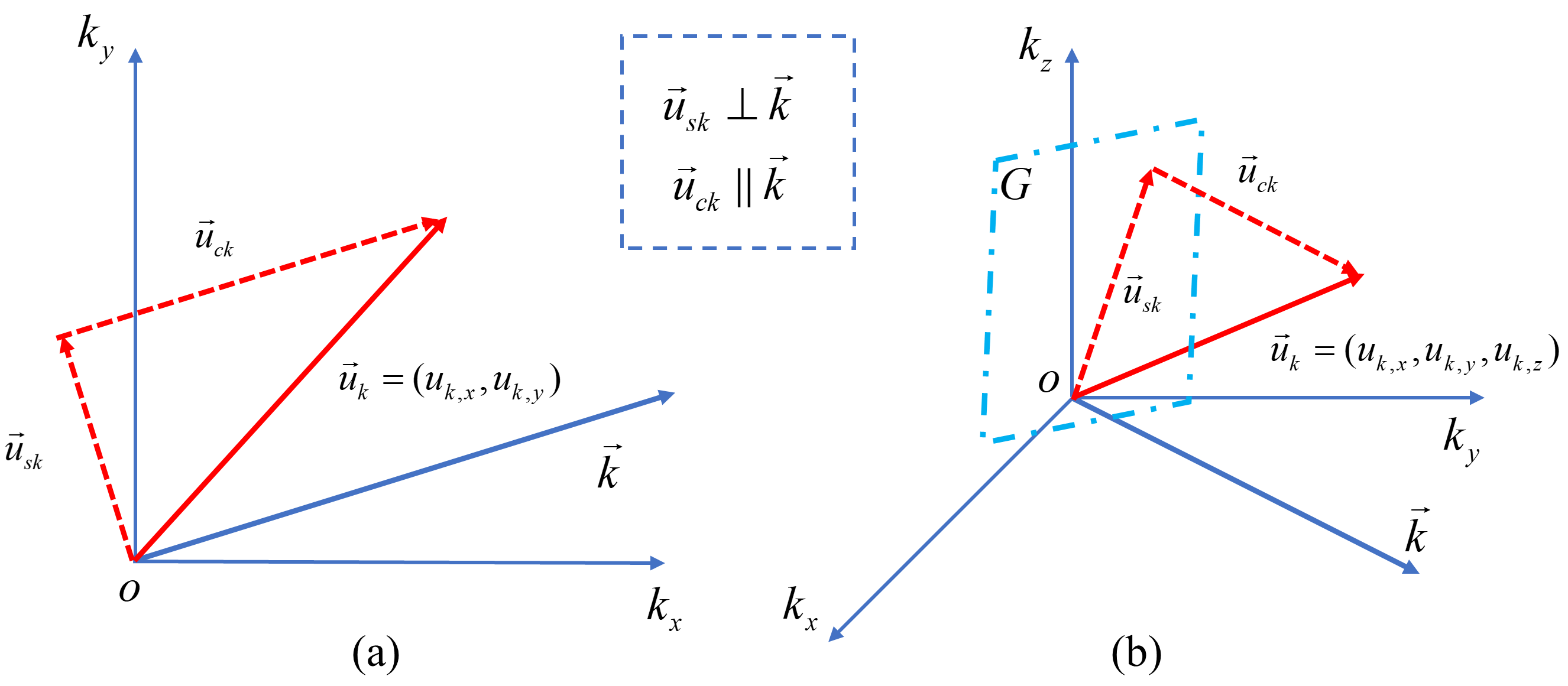
Figure 1: Sketch (in wavenumber space) showing the decomposition of the fluctuating velocity field ${{\vec{u}}_{k}}=\left({{u}_{k,i}}\right)$ into the solenoidal component ${{\vec{u}}_{sk}}$ and the compressible component ${{\vec{u}}_{ck}}$, for 2D (a) and 3D (b) cases. In panel (b), ${{\vec{u}}_{sk}}$ lies in the plane $G$, which is perpendicular to $\vec{k}$.

To calculate the energy spectra of $\vec{u}_{c}^{\text{th}}$ and $\vec{u}_{s}^{\text{th}}$, note that in wavenumber space, each independent velocity component $u_{k,i}^{\text{th}}$ shares the same amount of energy, given as

$${{\left|u_{k,i}^{\text{th}}\right|}^{2}}=\mathcal{F}\left\{\mathcal{R}_{{{u}_{i}}}^{\text{th}}\right\}={{{k}_{B}}\left\langle T\right\rangle}/{\left\langle\rho\right\rangle}\;.$$ (16)

Therefore, it follows that ${{\left|{{{\vec{u}}}^{\text{th}}}_{sk}\right|}^{2}}={{\left|{{{\vec{u}}}^{\text{th}}}_{ck}\right|}^{2}}$ for 2D cases, while ${{\left|{{{\vec{u}}}^{\text{th}}}_{sk}\right|}^{2}}=2{{\left|{{{\vec{u}}}^{\text{th}}}_{ck}\right|}^{2}}$ for 3D cases. The energy spectra of $\vec{u}_{c}^{\text{th}}$ and $\vec{u}_{s}^{\text{th}}$ can then be calculated from ${{E}^{\text{th}}}(k)$ as

$$\begin{dcases}\begin{array}[]{*{35}{l}}2\text{D}:&E_{c}^{\text{th}}(k)=E_{s}^{\text{th}}(k)=\frac{1}{2}{{E}^{\text{th}}}(k)\\ 3\text{D}:&E_{c}^{\text{th}}(k)=\frac{1}{2}E_{s}^{\text{th}}(k)=\frac{1}{3}{{E}^{\text{th}}}(k)\\ \end{array}\end{dcases}.$$ (17)

3 Simulation method

In this work, the unified stochastic particle (USP) method is employed to simulate the compressible decaying isotropic turbulence. Here we provide a brief description of the theoretical background and the basic algorithm of USP, and we refer readers to the original papers (Fei et al., 2019; Fei & Jenny, 2021; Fei et al., 2021) for details.

3.1 Governing equations

According to the gas kinetic theory, the state of a gas can be described by the velocity distribution function (VDF) $f(\vec{c};\vec{r},t)$, which is defined as the number density of molecules with velocity $\vec{c}$ at position $\vec{r}$ and time $t$. The evolution of VDF can be described by the Boltzmann equation (Bird, 1994):

$$\frac{\partial f}{\partial t}+\vec{c}\cdot\nabla f=Q\left(f,{{f}^{*}}\right),$$ (18)

where the term $\vec{c}\cdot\nabla f$ describes the change of VDF due to the convection of molecules, and $Q\left(f,{{f}^{*}}\right)$ is an integral that describes the intermolecular collisions. Due to the challenges associated with directly solving the Boltzmann equation, most numerical works are based on its model equations like the Bhatnagar-Gross-Krook (BGK) model (Bhatnagar et al., 1954) or the Shakhov-BGK (S-BGK) model (Shakhov, 1968). These models simplify the Boltzmann collision integral with a linear relaxation term, i.e.,

$$\frac{\partial f}{\partial t}+\vec{c}\cdot\nabla f=\frac{{{f}_{t}}-f}{{{\tau}_{r}}},$$ (19)

where the right-hand side of (19) describes the relaxation of VDF towards a target distribution function ${{f}_{t}}$ with the relaxation time ${{\tau}_{r}}$ comparable to the molecular mean collision time ${{\tau}_{mic}}$. In BGK and S-BGK models, the target distribution functions are given by the local macroscopic quantities as (Yao et al., 2023)

$${{f}_{t}}^{\text{BGK}}={{f}_{M}}=n{{\left(\frac{1}{2\pi RT}\right)}^{\frac{3}{2}}}\exp\left(-\frac{{{C}^{2}}}{2RT}\right),$$ (20)

$${{f}_{t}}^{\text{S-BGK}}={{f}_{M}}\left[1+(1-Pr)\frac{{{C}_{i}}{{q}_{i}}}{5PRT}\left(\frac{{{C}^{2}}}{2RT}-\frac{5}{2}\right)\right],$$ (21)

where $\vec{C}=\vec{c}-\vec{u}$ is the molecular thermal velocity, $R$ is the specific gas constant, $Pr$ is the Prandtl number, and ${{q}_{i}}$ is the heat flux. Compared with the original BGK model with a fixed $Pr$ of 1, the S-BGK model can be applied to gas flows with arbitrary $Pr$ (Yao et al., 2023).

3.2 Unified stochastic particle method

So far, the direct simulation Monte Carlo (DSMC) method (Bird, 1994) is still the most commonly used molecular method for simulating rarefied gas flows, and it has recently been employed to investigate the effect of thermal fluctuations on turbulence (McMullen et al., 2022b, 2023; Ma et al., 2023). A typical DSMC simulation tracks an appropriate number of “particles” (simulated molecules) in the computational domain. Each particle statistically represents a fixed number $F$ of identical real molecules, and $F$ is the so-called simulation ratio (Gallis et al., 2017; McMullen et al., 2022b). The domain is divided into computational cells where local macroscopic quantities are obtained by sampling particle information.

The key point of the DSMC method is that the effects of molecular movements and collisions are assumed uncoupled within a computational time step $\Delta t$. Specifically, the simulated particles move ballistically first, then the particles within the same cell are randomly chosen as collision pairs to assign new velocities according to the phenomenological collision models (Bird, 1994). DSMC can be regarded as an operator splitting scheme to solve the Boltzmann equation (Wagner, 1992; Feng et al., 2023), i.e.,

$$\begin{array}[]{*{35}{l}}\frac{\partial f}{\partial t}=-\vec{c}\cdot\nabla f,\\[2.84526pt] \frac{\partial f}{\partial t}=Q\left(f,{{f}^{*}}\right).\\ \end{array}$$ (22)

The same procedure can also be applied to (19), resulting in the governing equations of the stochastic particle (SP) method based on the BGK model (Gallis & Torczynski, 2000; Macrossan, 2001; Pfeiffer, 2018), given by

$$\begin{array}[]{*{35}{l}}\frac{\partial f}{\partial t}=-\vec{c}\cdot\nabla f,\\[2.84526pt] \frac{\partial f}{\partial t}=\frac{{{f}_{t}}-f}{{{\tau}_{r}}}.\\ \end{array}$$ (23)

In the SP method, the process of molecular movements is the same as that in the DSMC method, while the process of intermolecular collisions in DSMC is replaced by a “redistribution phase” where a fraction $(1-\exp\left(-{\Delta t}/{{{\tau}_{r}}}\;\right))$ of particles in each cell are randomly selected to assign new velocities according to ${{f}_{t}}$. The velocities of the remaining fraction of particles are unchanged.

Theoretically, it has been proved that DSMC and SP will produce unphysical momentum and energy transport if the time step $\Delta t$ and cell size $\Delta{{L}_{cell}}$ exceed ${{\tau}_{mic}}$ and ${{\lambda}_{mic}}$, respectively (Alexander et al., 1998; Hadjiconstantinou, 2000; Fei et al., 2019). To address this issue, the USP method supplements the effect of intermolecular collisions in the convection step. The corresponding governing equations based on the S-BGK model can be written as

$$\begin{array}[]{*{35}{l}}\frac{\partial f}{\partial t}=-\vec{c}\cdot\nabla f+{Q}^{*},\\[2.84526pt] \frac{\partial f}{\partial t}=\frac{{{f}_{t}}^{S-BGK}-f}{{{\tau}_{r}}}-{Q}^{*},\\ \end{array}$$ (24)

where ${Q}^{*}$ is a modified collision term closed by the Grad’s 13 moment distribution function (Fei et al., 2019). To make the USP method easier to be implemented, (24) can be further rewritten as (Fei & Jenny, 2021)

$$\begin{array}[]{*{35}{l}}\frac{\partial f}{\partial t}=-\vec{c}\cdot\nabla f,\\[2.84526pt] \frac{\partial f}{\partial t}=\frac{{{f}_{U}}-f}{{{\tau}_{r}}},\\ \end{array}$$ (25)

where ${{f}_{U}}$ is a new target distribution function given as

$${{f}_{U}}={{f}_{M}}\left[1+{{\varPsi}_{1}}\frac{{{\sigma}_{ij}}{{C}_{<i}}{{C}_{j>}}}{2PRT}+{{\varPsi}_{2}}\frac{2{{C}_{i}}{{q}_{i}}}{5PRT}\left(\frac{{{C}^{2}}}{2RT}-\frac{5}{2}\right)\right],$$ (26)

where ${{\varPsi}_{1}}$ and ${{\varPsi}_{2}}$ are related to $\Delta t$ as ${{\varPsi}_{1}}=1-{\Delta t}/{2{{\tau}_{r}}\coth\left({\Delta t}/{2{{\tau}_{r}}}\right)}$ and ${{\varPsi}_{2}}=1-{Pr\Delta t}/{2{{\tau}_{r}}\coth\left({\Delta t}/{2{{\tau}_{r}}}\right)}$, respectively. Based on (25), it follows that the implementation of USP is quite similar to that of SP. Theoretically, it has been demonstrated that the USP method has second-order temporal accuracy when $\Delta t\gg{{\tau}_{mic}}$ (Fei & Jenny, 2021). Furthermore, the second-order spatial accuracy can be achieved by a spatial interpolation procedure for macroscopic variables (Fei et al., 2021).

In this work, we simulate turbulent flows of the argon gas with $Pr={2}/{3}$ and $\gamma={5}/{3}$. The dynamic viscosity $\mu$ is assumed to depend on the temperature with a power-law exponent $\omega$, i.e.,

$$\mu={{\mu}_{ref}}{{\left(\frac{T}{{{T}_{ref}}}\right)}^{\omega}},$$ (27)

where ${{\mu}_{ref}}$ is the reference viscosity at the reference temperature ${{T}_{ref}}$. Specifically for argon gas, $\omega$, ${{\mu}_{ref}}$ and ${{T}_{ref}}$ are set to 0.81, $2.117\times{{10}^{-5}}\;\text{Pa}\cdot\text{s}$ and $273.15\;\text{K}$, respectively (Bird, 1994). The USP simulations are performed using the open-source code SPARTACUS (Feng et al., 2023), which has been recently developed by the authors within the framework of a widely used DSMC solver SPARTA (Plimpton et al., 2019). The performance of SPARTACUS has been evaluated over a series of test cases covering 1D to 3D flows with a wide range of Knudsen numbers and Mach numbers (Feng et al., 2023).

4 Two-dimensional turbulence

In a recent study (Ma et al., 2023), we employed the DSMC method to investigate the effect of thermal fluctuations on the spectra of 2D decaying isotropic turbulence. In this section, we use the DSMC results as benchmarks to validate the applicability of the USP method. The simulations begin with argon gas flows at ${{T}_{0}}=300\;\text{K}$ and ${{P}_{0}}=1\;\text{bar}$, with the number density calculated as ${{n}_{0}}={{{P}_{0}}}/{\left({{k}_{B}}{{T}_{0}}\right)}$. Based on these initial conditions, the molecular mean collision time ${{\tau}_{mic0}}$ and the molecular mean free path ${{\lambda}_{mic0}}$ are estimated using the variable hard sphere (VHS) model parameters specific to argon (Bird, 1994). The side lengths of the simulation domain are set to $\left({{L}_{x}},{{L}_{y}},{{L}_{z}}\right)=\left(4000{{\lambda}_{mic0}},4000{{\lambda}_{mic0}},40{{\lambda}_{mic0}}\right)$, and the domain is divided into uniform computational cells along the $x$ and $y$ directions for 2D simulations.

The initial turbulent velocity field is generated as follows. First, a divergence-free velocity field $\vec{u}_{0}^{\text{NS}}$ with a prescribed energy spectrum is randomly generated using the transfer procedures provided by Ishiko et al. (2009). The initial energy spectrum is specified as

$${{E}^{\text{NS}}}(k,t=0)=\frac{{{a}_{s}}}{2}\frac{U_{0}^{2}}{{{k}_{p}}}{{\left(\frac{k}{{{k}_{p}}}\right)}^{2s+1}}\text{exp}\left[-(s+\frac{1}{2}){{\left(\frac{k}{{{k}_{p}}}\right)}^{2}}\right],{{a}_{s}}=\frac{{{(2s+1)}^{s+1}}}{{{2}^{s}}s!},$$ (28)

where ${{U}_{0}}={{\left\langle{{\left(\vec{u}_{0}^{\text{NS}}\right)}^{2}}\right\rangle}^{0.5}}$ is the root mean square value of $\vec{u}_{0}^{\text{NS}}$, $s$ is a shape parameter of the spectrum, and ${{k}_{p}}$ is the wavenumber at which the spectrum has peak value. In this work, we take $s=3$ and ${{k}_{p}}=9{{k}_{\text{min}}}$, where ${{k}_{\text{min}}}={2\pi}/{L}\;$ is the minimum wavenumber, and $L={{L}_{x}}={{L}_{y}}$. Based on (28), the initial enstrophy is calculated as ${{\varOmega}_{0}}=\int_{0}^{\infty}{{{k}^{2}}{{E}^{\text{NS}}}(k)dk}$ (Herring et al., 1974). The enstrophy dissipation rate and the corresponding dissipation length scale are calculated as ${{\varepsilon}_{\varOmega 0}}=2{{\nu}_{0}}\int_{0}^{\infty}{{{k}^{4}}{{E}^{\text{NS}}}(k)dk}$ and ${{\eta}_{\varOmega 0}}={{\left({{{\nu}_{0}}^{3}}/{{{\varepsilon}_{\varOmega 0}}}\;\right)}^{{1}/{6}\;}}$, respectively (Herring et al., 1974). The initial turbulent Mach number and the Taylor Reynolds number are given by

$${{M}_{t0}}=\frac{{{U}_{0}}}{\left\langle\sqrt{\gamma RT}\right\rangle},R{{e}_{\lambda 0}}={{{\varOmega}_{0}}^{1.5}}/{{{\varepsilon}_{\varOmega 0}}}\;,$$ (29)

respectively.

The macroscopic velocity ${{\vec{u}}_{0}}^{\text{NS}}$ generated for each computational cell can be considered as the initial solution of deterministic NS equations without thermal fluctuations. The velocities ${{\vec{c}}_{0}}$ of USP particles in each cell are then generated based on the relation ${{\vec{c}}_{0}}={{\vec{u}}_{0}}^{\text{NS}}+{{\vec{C}}_{0}}$, where the particle thermal velocities ${{\vec{C}}_{0}}$ are randomly sampled from the Maxwell distribution function at $\left({{T}_{0}},{{n}_{0}}\right)$. This procedure enables the initial velocity field in the USP simulation to be expressed as $\vec{u}_{0}^{\text{USP}}=\vec{u}_{0}^{\text{NS}}+\vec{u}_{0}^{\text{th}}$ (McMullen et al., 2023), where $\vec{u}_{0}^{\text{th}}$ represents the thermal velocity fluctuation measured at each cell.

In this section, all simulation cases commence with the same turbulent velocity field with ${{M}_{t0}}=1$ and $R{{e}_{\lambda 0}}=23.3$. The other simulated parameters are shown in table 1. The DSMC simulation is conducted using SPARTA with $\Delta t=0.2{{\tau}_{mic0}}$ and $\Delta{{L}_{cell}}=0.49{{\lambda}_{mic0}}$. In contrast, the USP simulations are conducted with larger $\Delta t$ and $\Delta{{L}_{cell}}$. The average number of simulated particles within each cell ($\left\langle{{N}_{p}}\right\rangle$) increases with $\Delta{{L}_{cell}}$ to maintain the total number of particles unchanged, resulting in the same simulation ratio of $F=1549$. Based on $\Delta{{L}_{cell}}$, we further calculate the resolution parameter ${{k}_{\max}}{{\eta}_{{{\varOmega}_{0}}}}$, where ${{k}_{\max}}={\pi}/{\Delta{{L}_{cell}}}={\pi{{N}_{c}}}/{L}$ denotes the largest wavenumber corresponding to the half of ${{N}_{c}}$ (Wang et al., 2017). Each simulation case is run on 1024 CPU cores with the total computation time shown in table 1, corresponding to the same physical time of $t=10.7{{t}_{0}}$, where ${{t}_{0}}={L}/{\left(\text{2}\pi{{U}_{0}}\right)}$. Compared to the DSMC method, the USP method shows a significant improvement in computation efficiency due to the increases in $\Delta t$ and $\Delta{{L}_{cell}}$.

Case	Resolution (${{N}_{c}}^{2}$)	$\left\langle{{N}_{p}}\right\rangle$	${\Delta t}/{{{\tau}_{mic0}}}\;$	${\Delta{{L}_{cell}}}/{{{\lambda}_{mic0}}}\;$	${{k}_{\max}}{{\eta}_{\varOmega 0}}$	Total computation time (hours)
DSMC	${{8192}^{2}}$	25	0.2	0.49	94.3	31.00
USP	${{4096}^{2}}$	100	0.5	0.98	47.1	10.50
USP	${{2048}^{2}}$	400	1.0	1.95	23.6	4.97
USP	${{1024}^{2}}$	1600	2.0	3.91	11.8	2.79

Table 1: Simulated parameters for 2D decaying isotropic turbulence. All the simulations are performed with the initial conditions of ${{T}_{0}}=300\;\text{K}$, ${{P}_{0}}=1\;\text{bar}$, ${{M}_{t0}}=1$ and $R{{e}_{\lambda 0}}=23.3$.

To investigate whether the USP method can correctly reflect the effect of thermal fluctuations on turbulence, we calculate the energy spectra $E(k)$ and the thermodynamic spectra ${{E}_{g}}(k)$, where $g$ represents temperature, number density or pressure. The results for different simulation cases are shown in figure 2, corresponding to the time points of $t=3{{t}_{0}}$ and $t=9{{t}_{0}}$. Note that these spectra should be calculated based on the instantaneous flow field with thermal fluctuations fully preserved (McMullen et al., 2022b). As shown in figure 2, the USP spectra agree well with the DSMC spectra in the low wavenumber range, suggesting that the USP method can yield consistent large-scale turbulent statistics with the DSMC method. Notably, all the USP spectra display linear growth with $k$ in the high wavenumber range, indicating the effect of thermal fluctuations. In figure 2, both the spectra obtained from DSMC and USP simulations align well with the theoretical spectra of thermal fluctuations, as described by (12) and (13) at high wavenumbers. Note that the theoretical spectra should be multiplied by the simulation ratio $F$, as the magnitude of thermal fluctuations in simulations depends on the number of simulated particles (Hadjiconstantinou, 2000; McMullen et al., 2022b).

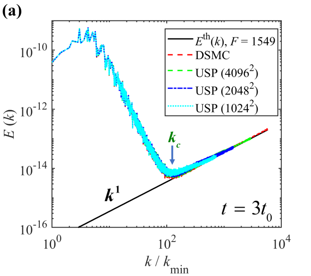
(a)

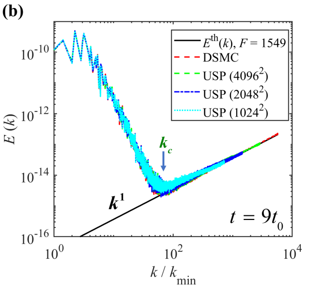
(b)

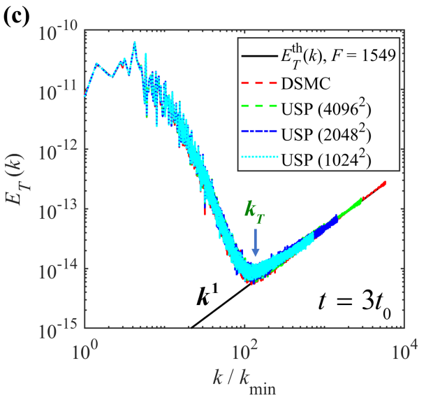
(c)

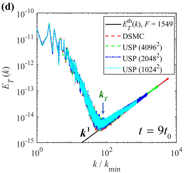
(d)

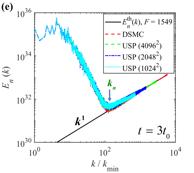
(e)

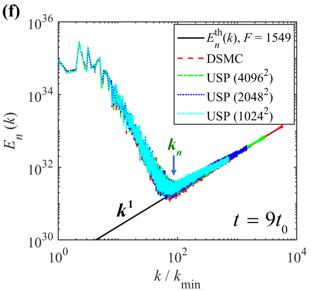
(f)

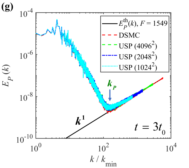
(g)

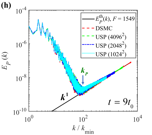
(h)

Figure 2: Energy spectra $E(k)$ and thermodynamic spectra (${{E}_{T}}(k)$, ${{E}_{n}}(k)$, ${{E}_{P}}(k)$) of 2D decaying turbulence at $t=3{{t}_{0}}$ (a, c, e, g) and $t=9{{t}_{0}}$ (b, d, f, h). The spectra of thermal fluctuations calculated from (12) and (13) are also displayed with $F$ = 1549.

We define ${{k}_{c}}$ and ${{k}_{g}}$ as the crossover wavenumbers (McMullen et al., 2022b; Bell et al., 2022; Ma et al., 2023) for $E(k)$ and ${{E}_{g}}(k)$, respectively. These wavenumbers give the length scales below which thermal fluctuations dominate the turbulent spectra. As shown in figure 2, the USP simulations at different resolutions yield identical crossover wavenumbers to those obtained by DSMC simulations. Additionally, a notable reduction in their values over time is observed when comparing the crossover wavenumbers at $t=3{{t}_{0}}$ and $t=9{{t}_{0}}$. As the crossover wavenumbers represent the length scales where turbulent fluctuations are “masked” by thermal fluctuations, it is expected that they decrease as the turbulent fluctuations continuously decay.

Using the Helmholtz decomposition (Samtaney et al., 2001), we can further investigate the effect of thermal fluctuations on the solenoidal and compressible velocity fields, respectively. Figure 3 presents the energy spectra of the velocity field $\vec{u}$ and its two components ${{\vec{u}}_{c}}$ and ${{\vec{u}}_{s}}$ at $t=3{{t}_{0}}$. The USP results correspond to the simulation resolution of $1024^{2}$. As can be seen from figure 3, the USP spectra coincide with the DSMC spectra over the full wavenumber range. More importantly, the energy spectra of ${{\vec{u}}_{c}}$ and ${{\vec{u}}_{s}}$ overlap in the high wavenumber region, which corroborates the conclusion drawn in § 2 that $\vec{u}_{c}^{\text{th}}$ and $\vec{u}_{s}^{\text{th}}$ satisfy the equipartition of energy in the 2D wavenumber space (see discussions before (17)). To summarize, the USP method can accurately capture the effect of thermal fluctuations on turbulence even with significantly larger time steps and cell sizes compared to the DSMC method.

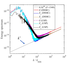
Figure 3: 2D energy spectra for the velocity field and its two components obtained by DSMC and USP ($1024^{2}$) at $t=3{{t}_{0}}$. The theoretical spectrum of thermal fluctuations is also displayed with $F$ = 1549.

5 Three-dimensional turbulence

In this section, we employ the USP method to simulate 3D decaying isotropic turbulence. The simulations begin with argon gas flows at ${{T}_{0}}=273.15\;\text{K}$ and ${{P}_{0}}=1\;\text{bar}$. The simulation domain is a cubic box with the side length of $L=2000{{\lambda}_{mic0}}$, and the periodic boundary conditions are applied in all three directions. Similar to the 2D turbulence simulations, the initial macroscopic velocity field $\vec{u}_{0}^{\text{USP}}$ is randomly generated following the relation $\vec{u}_{0}^{\text{USP}}=\vec{u}_{0}^{\text{NS}}+\vec{u}_{0}^{\text{th}}$, where $\vec{u}_{0}^{\text{NS}}$ is a divergence–free velocity field which satisfies the deterministic NS equations, and $\vec{u}_{0}^{\text{th}}$ represents the thermal fluctuations.

In this work, $\vec{u}_{0}^{\text{NS}}$ follows the special form of the energy spectrum as

$${{E}^{\text{NS}}}(k,t=0)=A{{k}^{4}}\text{exp}\left[-2{{\left(\frac{k}{{{k}_{p}}}\right)}^{2}}\right],A=\frac{32}{3\sqrt{2\pi}}\frac{{{U}_{0}}^{2}}{{{k}_{p}}^{5}},$$ (30)

where ${{k}_{p}}$ is the peak wavenumber, and ${{U}_{0}}$ is the root mean square value of $\vec{u}_{0}^{\text{NS}}$, i.e., ${{U}_{0}}={{\left\langle{{\left(\vec{u}_{0}^{\text{NS}}\right)}^{2}}\right\rangle}^{0.5}}$. In this work, we take ${{k}_{0}}=4{{k}_{\min}}$, where ${{k}_{\text{min}}}={2\pi}/{L}\;$ is the minimum wavenumber. Based on (30), the longitudinal integral length scale and the large eddy turnover time are given by (Chen et al., 2020)

$${{L}_{f0}}=\frac{3\pi}{2{{U}_{0}}^{2}}\int_{0}^{\infty}{\frac{{{E}^{\text{NS}}}(k)}{k}dk},{{T}_{e0}}=\frac{\sqrt{3}{{L}_{f}}}{{{U}_{0}}},$$ (31)

respectively. The initial dissipation rate and the Kolmogorov length scale are calculated as

$${{\varepsilon}_{0}}=2{{\nu}_{0}}\int_{0}^{\infty}{{{k}^{2}}{{E}^{\text{NS}}}(k)dk},{{\eta}_{0}}={{\left({{{\nu}_{0}}^{3}}/{{{\varepsilon}_{0}}}\;\right)}^{{1}/{4}\;}},$$ (32)

respectively. The initial turbulent Mach number ${{M}_{t0}}$ is calculated using (29), and the initial Taylor microscale ${{\lambda}_{0}}$ and the corresponding Reynolds number are given by (Pope, 2000)

$${{\lambda}_{0}}=\sqrt{\frac{5{{\nu}_{0}}{{U}_{0}}^{2}}{{{\varepsilon}_{0}}}},R{{e}_{\lambda 0}}=\frac{{{U}_{0}}{{\lambda}_{0}}}{\sqrt{3}{{\nu}_{0}}},$$ (33)

respectively.

Table 2 shows the parameters of USP simulations, where ${{M}_{t0}}$ ranges from 0.6 to 0.9, and $R{{e}_{\lambda 0}}$ increases with ${{M}_{t0}}$. Based on the discussions in § 4, the USP simulations are performed with larger time steps and cell sizes compared to those typically used in DSMC simulations. The average number of simulated particles per cell is 100, resulting in a total of 13.42 billion particles, each of which represents 1838 real molecules.

Resolution (${{N}_{c}}^{3}$)	$R{{e}_{\lambda 0}}$	${{M}_{t0}}$	${{{L}_{f0}}}/{{{\eta}_{0}}}\;$	$\left\langle{{N}_{p}}\right\rangle$	${\Delta t}/{{{\tau}_{mic0}}}\;$	${\Delta{{L}_{cell}}}/{{{\lambda}_{mic0}}}\;$	${{k}_{\max}}{{\eta}_{0}}$
${{512}^{3}}$	68.8	0.6	20.5	100	1	3.9	7.84
${{512}^{3}}$	86.1	0.75	22.9	100	0.8	3.9	7.01
${{512}^{3}}$	103.3	0.9	25.1	100	0.8	3.9	6.40

Table 2: USP simulation parameters for 3D decaying isotropic turbulence. All the simulations are performed with the initial conditions of ${{T}_{0}}=273.15\;\text{K}$ and ${{P}_{0}}=1\;\text{bar}$.

In addition to the USP simulations, we numerically solved the 3D deterministic compressible NS equations using the direct numerical simulation (DNS) method (Pope, 2000). The effect of thermal fluctuations on turbulence can then be analyzed by comparing the USP and DNS results. Specifically, three DNS cases are performed with the same $R{{e}_{\lambda 0}}$ and ${{M}_{t0}}$ as USP simulations. The gas thermodynamic properties in DNS are identical to those in USP simulations. The initial values of $\rho$, $T$, and $P$ are uniformly set within the DNS domain, and the initial velocity field is directly obtained from $\vec{u}_{0}^{\text{NS}}$ generated during the USP initialization procedures. For the numerical scheme of DNS, considering that ${{M}_{t0}}$ is high, we utilize a hybrid scheme proposed by Wang et al. (2010), which combines an eighth-order compact central finite difference scheme (Lele, 1992) for smooth regions and a seventh-order weighted essentially non-oscillatory (WENO) scheme (Balsara & Shu, 2000) for shock regions. The time steps for all the DNS cases are smaller than 0.001${{T}_{e0}}$, and the space resolutions in DNS are the same as those in USP simulations (see table 2). Previous grid refinement studies of the hybrid scheme (Wang et al., 2011, 2012) have shown that the resolution parameters ${{k}_{\max}}{{\eta}_{0}}\geq 3.3$ are enough for the convergence of turbulent statistics.

5.1 Basic turbulent statistics

In previous studies employing the DSMC method (McMullen et al., 2022b, 2023), researchers have demonstrated the statistical independence between thermal fluctuations and turbulent fluctuations predicted by the deterministic NS equations. Consequently, it is anticipated that the mean square fluctuations in USP simulations at a given time can be expressed as $\left\langle{{\left(\delta{{a}^{\text{USP}}}\right)}^{2}}\right\rangle=\left\langle{{\left(\delta{{a}^{\text{DNS}}}\right)}^{2}}\right\rangle+\left\langle{{\left(\delta{{a}^{\text{th}}}\right)}^{2}}\right\rangle$, where $\delta{{a}^{\text{DNS}}}$ represents the turbulent fluctuations predicted by the DNS method. To illustrate this relation, figure 4 presents the simulation results for the turbulent kinetic energy $K$ and the mean square pressure fluctuations $P_{ms}$ in the case of $R{{e}_{\lambda 0}}$= 103.3 and ${{M}_{t0}}$= 0.9. $K$ is normalized by the initial value of DNS, and $P_{ms}$ is normalized by the square of initial pressure. As observed in figure 4, the results obtained from USP simulations (solid lines) are notably larger than those obtained from DNS (dotted lines), indicating the presence of thermal fluctuations, and the corresponding results (${{K}^{\text{th}}}$ and $P_{ms}^{\text{th}}$) can be obtained at each time point using (3) and (6) with $F=1838$. By subtracting ${{K}^{\text{th}}}$ and $P_{ms}^{\text{th}}$ directly from the USP results, we obtain results (dash-dotted lines) that perfectly align with those obtained from DNS. Note that the effects of thermal fluctuations can also be reduced by averaging the USP flow field over time intervals that are long compared to the simulation time step $\Delta t$ but short compared to the Kolmogorov time scale ${{\tau}_{\eta}}$ (Gallis et al., 2021). The USP results obtained after this short-time average procedure are also shown in figure 4 (dashed lines), which are in good agreement with the DNS results.

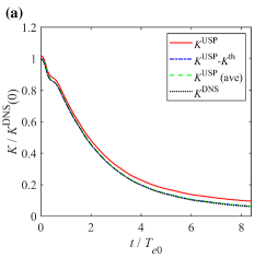
(a)

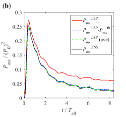
(b)

Figure 4: Time evolution of (a) normalized turbulent kinetic energy, and (b) normalized mean square value of pressure fluctuations, for the case with $R{{e}_{\lambda 0}}$= 103.3 and ${{M}_{t0}}$= 0.9.

Figures 5(a)–(c) show the temporal evolutions of ${K}/{K(0)}$, ${{{P}_{ms}}}/{\left({{P}_{0}}\right)^{2}}$ and $M_{t}$ obtained from both USP and DNS simulations for cases with different ${{M}_{t0}}$. The USP results correspond to the short-time average flow field. In figure 5(a), since the time histories of ${K}/{K(0)}$ for different ${{M}_{t0}}$ almost overlap, only the results for ${{M}_{t0}}=0.6$ and ${{M}_{t0}}=0.9$ are presented. As observed from figures 5(a)–(c), the USP results exhibit excellent agreement with the DNS results throughout the entire time range. For cases with higher ${{M}_{t0}}$, the fluctuations of thermodynamic variables are amplified to greater magnitudes due to the increase of compressibility. To further validate the accuracy of USP simulations, we compare the probability density functions (PDFs) of the local Mach number $M{{a}_{loc}}$ obtained from both the USP and DNS simulations. $M{{a}_{loc}}$ is defined as (Samtaney et al., 2001; Chen et al., 2020)

$$M{{a}_{loc}}=\frac{{{\left(\vec{u}\cdot\vec{u}\right)}^{{1}/{2}\;}}}{\sqrt{\gamma RT}}.$$ (34)

Figure 5(d) shows the PDFs at $t=1.4{{T}_{e0}}$, where the USP results exhibit good agreement with the DNS results across all three cases.

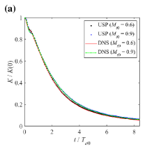
(a)

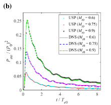
(b)

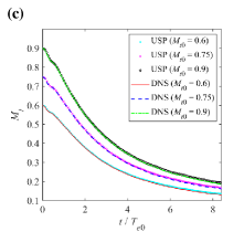
(c)

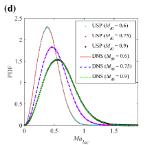
(d)

Figure 5: Panels (a)–(c) display the time evolutions of normalized turbulent kinetic energy, normalized mean square pressure fluctuations and turbulent Mach number, respectively. Panel (d) displays the PDFs of the local Mach number at $t=1.4{{T}_{e0}}$. All the USP results are obtained based on the short-time average flow field without thermal fluctuations.

5.2 Effect of thermal fluctuations on spectra

In previous relevant numerical studies on 3D turbulence (Bell et al., 2022; McMullen et al., 2022b, 2023), researchers mainly focused on the effect of thermal fluctuations on the spectra of the velocity field $\vec{u}$. By employing the Helmholtz decomposition, we can further consider the effect of thermal fluctuations on spectra of the solenoidal and compressible velocity components (i.e., ${{\vec{u}}_{s}}$ and ${{\vec{u}}_{c}}$). Figure 6 presents the USP and DNS spectra of $\vec{u}$, ${{\vec{u}}_{c}}$ and ${{\vec{u}}_{s}}$ at $t=1.4{{T}_{e0}}$, for the case of ${{M}_{t0}}=0.9$. The spectra are plotted against the dimensionless wavenumber ${k}/{{{k}_{\min}}}$. Except for being slightly noisy, the USP spectra agree well with the DNS spectra at small wavenumbers. In the high wavenumber range, the DNS spectra exhibit a continuous decrease, whereas the USP spectra exhibit a quadratic growth with respect to $k$, which corresponds to the effect of thermal fluctuations (Bell et al., 2022; McMullen et al., 2022b; Bandak et al., 2022). In figure 6, we further compare $E(k)$, ${{E}_{c}}(k)$ and ${{E}_{s}}(k)$ obtained by USP at large wavenumbers (see the inset), illustrating the relation of $E(k)=1.5{{E}_{s}}(k)=3{{E}_{c}}(k)$. The USP results support the conclusion drawn in § 2 that the energy of $\vec{u}_{s}^{\text{th}}$ is twice the energy of $\vec{u}_{c}^{\text{th}}$ in the wavenumber space (see discussions before (17)).

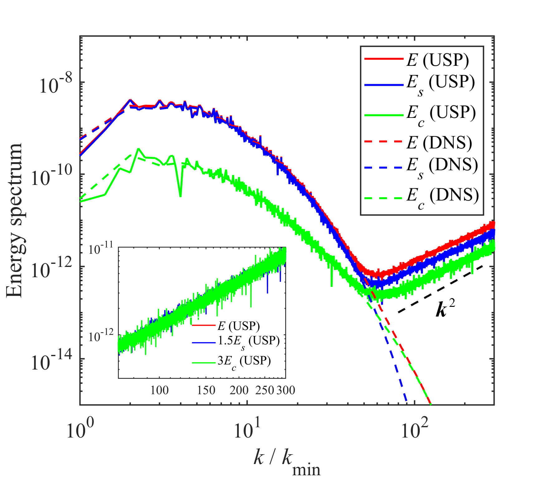
Figure 6: Energy spectra for the velocity field and its two components obtained from USP and DNS simulations at $t=1.4{{T}_{e0}}$, for the case of $R{{e}_{\lambda 0}}$= 103.3 and ${{M}_{t0}}$= 0.9. The inset shows the relationship between $E(k)$, ${{E}_{c}}(k)$ and ${{E}_{s}}(k)$ obtained from USP simulations at large wavenumbers.

In figure 7, we present $E(k)$, ${{E}_{s}}(k)$ and ${{E}_{c}}(k)$ obtained from USP and DNS simulations at $t=1.4{{T}_{e0}}$ under different ${{M}_{t0}}$ conditions, in order to study the effect of compressibility on spectra. The spectra are plotted against the dimensionless wavenumber $k\eta$, where $\eta$ is the Kolmogorov length scale obtained by DNS. The crossover wavenumbers ${{k}_{c}}$, $k_{c}^{s}$ and $k_{c}^{c}$ are estimated as the intersections of $E(k)$, ${{E}_{s}}(k)$ and ${{E}_{c}}(k)$ obtained by DNS with the thermal fluctuation spectra (McMullen et al., 2022b).

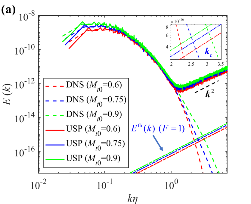
(a)

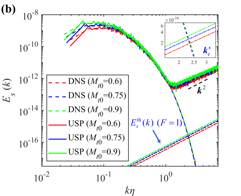
(b)

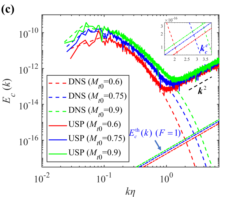
(c)

Figure 7: $E(k)$ (a), ${{E}_{s}}(k)$ (b) and ${{E}_{c}}(k)$ (c) obtained from USP and DNS simulations at $t=1.4{{T}_{e0}}$, for cases with different ${{M}_{t0}}$. The thermal fluctuation spectra with $F$ = 1 are also shown for comparison. The insets are the enlarged views showing the intersection points between thermal fluctuation spectra and DNS spectra (i.e., the crossover wavenumbers for the real gases).

According to the discussions in § 4, the thermal fluctuation spectra obtained by USP simulations are overestimated due to the use of a simulation ratio $F>\text{1}$. By setting $F$ = 1, we can obtain the spectra of thermal fluctuations corresponding to the real gases. As observed from figure 7(a), ${{k}_{c}}\eta$ lies between 2.3 and 3 for $F=1$, corresponding to ${\eta}/{{{l}_{c}}}$ in the range of 0.37 to 0.48 (${{l}_{c}}={2\pi}/{{{k}_{c}}}$), indicating that thermal fluctuations dominate $E(k)$ at spatial scales slightly larger than the Kolmogorov length scale. The similar results were also reported by McMullen et al. (2022b) and Bell et al. (2022) in their simulations of 3D turbulence, where they found ${\eta}/{{{l}_{c}}}\approx 0.5$. More interestingly, with the increase of ${{M}_{t}}$, it is noteworthy that $k_{c}^{s}\eta$ remains relatively stable around 2.3 (see figure 7(b)), whereas $k_{c}^{c}\eta$ changes significantly from 2.1 to 3.3 (see figure 7(c)). This observation suggests that the influence of thermal fluctuations on ${{\vec{u}}_{c}}$ is more responsive to changes in compressibility compared to that on ${{\vec{u}}_{s}}$. Despite the USP simulations being performed with a large simulation ratio ($F$ = 1838), the trends of the crossover wavenumbers predicted by USP are completely consistent with those observed in real gases.

Since compressible turbulent flows own significant features of the fluctuations in thermodynamic variables, it is of interest to study their spectra under the presence of thermal fluctuations. Figure 8 shows the spectra of $T$, $n$ and $P$ obtained by USP and DNS simulations at $t=1.4{{T}_{e0}}$ for different cases, where the USP spectra grow quadratically with $k$ in the high wavenumber range, indicating the effect of thermal fluctuations. Following the previous discussions, we calculate the thermal fluctuation spectra with $F$ = 1 to obtain the crossover wavenumbers ${{k}_{T}}$, ${{k}_{n}}$ and ${{k}_{P}}$ for the real gas flows. It is interesting to observe that as ${{M}_{t}}$ increases, the ranges of variation for ${{k}_{T}}\eta$, ${{k}_{n}}\eta$ and ${{k}_{P}}\eta$ are (2.1, 3.1), (2.1, 3.3) and (2.1, 3.5), respectively, which are close to the aforementioned trend observed for $k_{c}^{c}\eta$. To further verify the coupling relationship between the spectra of thermodynamic variables and the spectrum of ${{\vec{u}}_{c}}$, in figure 9 we present the corresponding USP results for the cases with ${{M}_{t0}}=0.6$ and ${{M}_{t0}}=0.9$, following the normalization rules that the integral of the spectrum over the entire wavenumber range is equal to 1. It can be seen that the spectra of all the thermodynamic variables show good agreement with ${{E}_{c}}(k)$, indicating that the spatial correlations of thermodynamic fluctuations are dominated by the compressible mode of the velocity field. It is worth noting that this phenomenon was also reported in our previous work where we simulated the 2D decaying isotropic turbulence using the DSMC method (Ma et al., 2023).

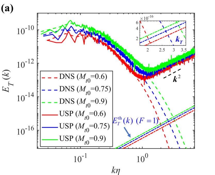
(a)

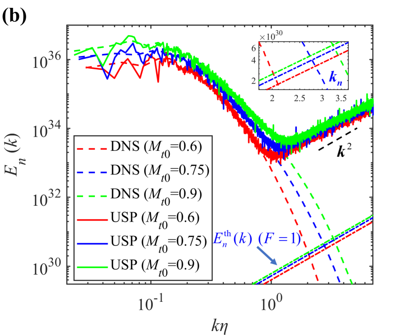
(b)

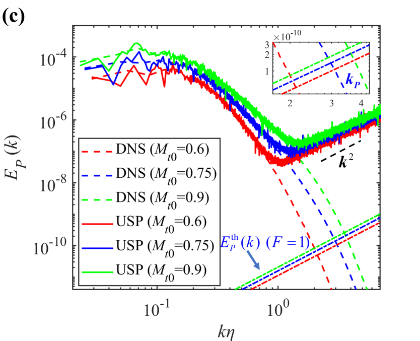
(c)

Figure 8: ${{E}_{T}}(k)$ (a), ${{E}_{n}}(k)$ (b) and ${{E}_{P}}(k)$ (c) obtained from USP and DNS simulations at $t=1.4{{T}_{e0}}$, for cases with different ${{M}_{t0}}$. The thermal fluctuation spectra with $F$ = 1 are also shown for comparison. The insets are the enlarged views showing the intersection points between thermal fluctuation spectra and DNS spectra (i.e., the crossover wavenumbers for the real gases).

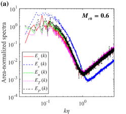
(a)

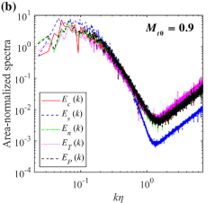
(b)

Figure 9: Normalized USP spectra of compressible velocity component, solenoidal velocity component, number density, temperature and pressure at $t=1.4{{T}_{e0}}$, for cases with ${{M}_{t0}}=0.6$(a) and ${{M}_{t0}}=0.9$(b).

6 Thermal fluctuations and the turbulence predictability

Our research above indicates that thermal fluctuations have a significant impact on the turbulent spectra at length scales comparable to the turbulent dissipation length scale. On the other hand, this suggests that the large-scale turbulence statistics are unaffected by thermal fluctuations. However, if we shift our focus to the turbulent flow field structures, the situation may be quite different. Considering the current experimental challenges in directly measuring thermal fluctuations in turbulent flows (Bandak et al., 2022), the initial state of thermal fluctuations remains unknown when we attempt to predict the subsequent evolution of turbulence. Due to the chaotic nature of turbulent flows, even tiny deviations in the initial thermal fluctuations may lead to the unpredictability of large-scale turbulence structures after a certain period of time (Ruelle, 1979).

In this section, we employ the USP method to study the predictability of compressible decaying isotropic turbulence for both 2D and 3D cases. The initial temperature and pressure of the simulation cases are consistent with those in the previous sections, and the other simulated parameters are shown in table 3. Note that the initial Taylor Reynolds number has different definitions for 2D and 3D turbulent flows, as shown in (29) and (33), respectively. Therefore, in table 3 we provide the initial global Reynolds number ${{{Re}}_{0}}$, which is given as

$$R{{e}_{0}}=\frac{{{U}_{0}}L}{2\pi{{\nu}_{0}}},$$ (35)

where $L$ is the side length of the simulation domain. Based on $L$, one can also calculate the initial global Knudsen numbers as $K{{n}_{0}}={{{\lambda}_{mic0}}}/{L}\;$.

Case	$K{{n}_{0}}$	${{Re}_{0}}$	${{M}_{t0}}$	Resolution	$\left\langle{{N}_{p}}\right\rangle$	$F$	${\Delta t}/{{{\tau}_{mic0}}}\;$	${\Delta{{L}_{cell}}}/{{{\lambda}_{mic0}}}\;$	${{k}_{\max}}{{\eta}_{\varOmega 0}}$ (${{k}_{\max}}{{\eta}_{0}}$)
2D	0.000125	1590	1.0	${{2048}^{2}}$	400	6194	2	3.9	18.7
3D	0.00025	954	1.2	${{1024}^{3}}$	25	7354	2	3.9	7.84

Table 3: USP simulation parameters for the study of turbulence predictability.

To investigate the effect of thermal fluctuations on the predictability of turbulence, note that the velocity field in a USP simulation is initialized as $\vec{u}_{0}^{\text{USP}}=\vec{u}_{0}^{\text{NS}}+\vec{u}_{0}^{\text{th}}$. Therefore, for both 2D and 3D cases, we can create an ensemble of realizations starting with the same $\vec{u}_{0}^{\text{NS}}$, but with different $\vec{u}_{0}^{\text{th}}$ generated using independent random number streams. This approach ensures that each realization initially differs from others solely due to small-scale thermal fluctuations.

Figure 10 shows the temporal evolution of the vorticity fields for two realizations of 2D decaying turbulence. Since we focus on the predictability of large-scale structures in turbulent flows, the contours are plotted based on “coarse-grained” cells with a lower resolution, i.e., the length of coarse-grained cells ${L}/{{{N}_{g}}}$ is much larger than the original cell length $\Delta{{L}_{cell}}$. As seen in figures 10(a) and (d), the vorticity fields of two realizations are identically the same at $t=0$, indicating that the thermal fluctuations have no effect on the initial large-scale turbulent structures. At $t=12.2{{t}_{0}}$, the vorticity fields of two realizations show slight differences (see figures 10(b) and (e)), and finally the vorticity fields show significant divergence at $t=18.3{{t}_{0}}$ (see figures 10(c) and (f)). For the 3D case, a similar phenomenon is observed in figure 11, where we compare the velocity magnitudes ${{U}_{mag}}$ of two realizations. At $t=16.9{{T}_{e0}}$, which corresponds to the ending time of 3D simulations, the velocity fields of the two realizations show observable differences (see figures 11(c) and (f)). Therefore, it can be concluded that the initial differences in small-scale thermal fluctuations will lead to the unpredictability of large-scale structures of turbulence after a certain period of time.

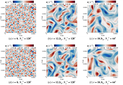
Figure 10: Temporal evolution of the vorticity field for 2D decaying turbulence with $R{{e}_{0}}$=1590 and ${{M}_{t0}}$=1. Panels (a-c) and (d-f) correspond to two realizations. The contours are plotted based on coarse-grained cells with a lower resolution (${{N}_{g}}^{2}$).

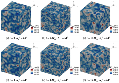
Figure 11: Temporal evolution of the velocity field for 3D decaying turbulence with $R{{e}_{0}}$=954 and ${{M}_{t0}}$=1.2. Panels (a-c) and (d-f) correspond to two realizations.The contours are plotted based on coarse-grained cells with a lower resolution (${{N}_{g}}^{3}$).

To quantify the divergence between different flow realizations, we define the local error velocity field as (Boffetta et al., 1997; Boffetta & Musacchio, 2017)

$${{\vec{u}}_{error}}(\vec{r},t)=\frac{1}{\sqrt{2}}({{\vec{u}}_{1}}(\vec{r},t)-{{\vec{u}}_{2}}(\vec{r},t)),$$ (36)

where ${{\vec{u}}_{1}}$ and ${{\vec{u}}_{2}}$ represent the velocity fields of two independent realizations. In figure 12, we compare the energy spectra of original velocity fields and error velocity fields at different time points for both 2D and 3D cases. The results are obtained by taking the ensemble average of three independent realizations. Since $\vec{u}_{0}^{\text{th}}$ in each pair of realizations can be considered as two sets of independent Gaussian random variables (Landau & Lifshitz, 1980), the initial error velocity field can be regarded as a new thermal fluctuation field with the same Gaussian statistics. As shown in figure 12, the error spectra ${{E}_{err}}$ at $t$ = 0 grow linearly/quadratically with $k$ for 2D/3D cases, reflecting the basic features of thermal fluctuations. As time progresses, ${{E}_{err}}$ is still dominated by thermal fluctuations in the high wavenumber region, while gradually approaching $E$ in the low wavenumber region. This indicates that the initial errors of thermal fluctuations propagate to the larger scales. It is worth noting that, the “inverse cascade” of the error velocity field has also been observed in the previous studies based on the deterministic NS equations (Métais & Lesieur, 1986; Boffetta et al., 1997; Boffetta & Musacchio, 2001, 2017; Berera & Ho, 2018), where the divergence of velocity field trajectories is achieved by initially introducing an artificial perturbation. Compared to these works, in our current research, the initial errors originate from thermal fluctuations, which are inherent properties of fluids. Furthermore, the influence of thermal fluctuations persists throughout the turbulent evolution process, rather than being limited to the initial moment.

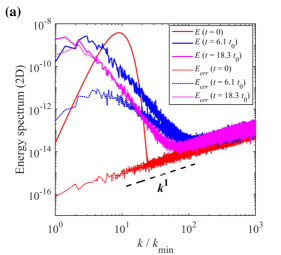
(a)

(b)

Figure 12: Energy spectra of the original velocity field and the error velocity field at different time points, for 2D (a) and 3D (b) cases.

In addition to the turbulent velocity field, we further investigate the effect of thermal fluctuations on the predictability of the turbulent thermodynamic field, and this aspect has not been reported in the literature. We define the local error fields of the thermodynamic variables as

$${{g}_{error}}(\vec{r},t)=\frac{1}{\sqrt{2}}({{g}_{1}}(\vec{r},t)-{{g}_{2}}(\vec{r},t)),$$ (37)

where $g$ stands for $T$, $n$ and $P$. Figure 13 presents a comparison between the spectra of the original temperature fields and the error temperature fields for both 2D and 3D cases. Similar comparisons can also be made for number density and pressure. At the beginning of USP simulations, the fluctuations of thermodynamic variables are solely attributed to thermal fluctuations, resulting in a complete coincidence between ${{E}_{T}}$ and ${{E}_{T,err}}$. Then, the compressibility of turbulence causes a rapid amplification of ${{E}_{T}}$ to a high magnitude in the low wavenumber region, while ${{E}_{T,err}}$ requires a considerably longer time to approach ${{E}_{T}}$. In figures 14 and 15, we present the temperature fields of two realizations at the end of the USP simulations for 2D and 3D cases, respectively. Compared to the 3D cases, the differences between the two realizations are more pronounced for the 2D cases, which can be supported by figure 13(a) where ${{E}_{T,err}}$ almost coincides with ${{E}_{T}}$ at the end of the simulation.

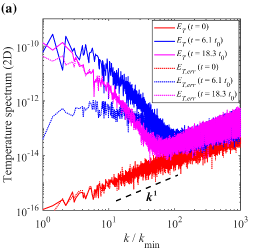
(a)

(b)

Figure 13: Spectra of the original temperature field and the error temperature field at different time points, for 2D (a) and 3D (b) cases.

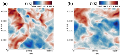
Figure 14: Temperature field for 2D decaying turbulence with $R{{e}_{0}}$=1590 and ${{M}_{t0}}$=1, at $t$ = 18.3$t_{0}$. Panels (a) and (b) correspond to two realizations.

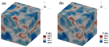
Figure 15: Temperature field for 3D decaying turbulence with $R{{e}_{0}}$=954 and ${{M}_{t0}}$=1.2, at $t$ = 16.9${{T}_{e0}}$. Panels (a) and (b) correspond to two realizations.

In § 5, we have discussed the coupling relationship between turbulent thermodynamic variables and the compressible velocity component (see figure 9). To see whether this relationship holds for the turbulent error field, we compare the corresponding area-normalized spectra for both 2D and 3D cases in figure 16. It is evident that the error spectra of all the thermodynamic variables are in good agreement with the spectrum of the compressible component of the error velocity field. This suggests that in decaying compressible turbulence, the predictabilities of the thermodynamic variables are closely related to the predictability of the compressible velocity component.

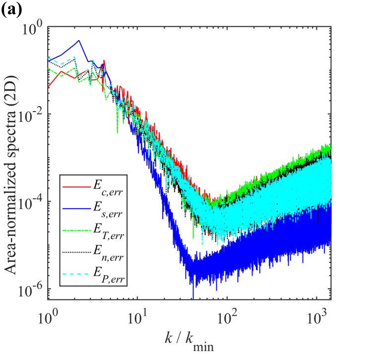
(a)

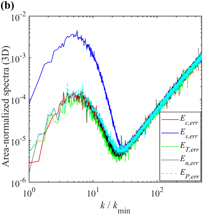
(b)

Figure 16: (a) Normalized error spectra of compressible velocity component, solenoidal velocity component, temperature, number density and pressure for 2D decaying turbulence at $t$ = 18.3$t_{0}$. (b) The error spectra corresponding to the 3D decaying turbulence at t = 16.9${{T}_{e0}}$.

7 Concluding remarks

In this work, we employed the USP method to numerically investigate the effects of thermal fluctuations on compressible decaying isotropic turbulence. Compared to the traditional molecular methods such as DSMC, USP can be applied with much larger time steps and cell sizes as it couples the effects of molecular movements and collisions.

In both 2D and 3D simulations, it is found that the turbulent spectra of velocity and thermodynamic variables are greatly affected by thermal fluctuations in the high wavenumber range. The wavenumber scaling law of the thermal fluctuation spectra depends on the spatial dimension $d$ as ${{k}^{(d-1)}}$. By applying the Helmholtz decomposition to the velocity field, we show that the thermal fluctuation spectra of solenoidal and compressible velocity components (i.e., ${{E}_{s}}(k)$ and ${{E}_{c}}(k)$) follow an energy ratio of 1:1 for 2D cases, while this ratio changes to 2:1 for 3D cases.

For 3D decaying turbulence, a comparative study was conducted between the USP method and the DNS method based on the deterministic NS equations. The crossover wavenumbers were determined as the intersections between DNS spectra and thermal fluctuation spectra. The results show that thermal fluctuations dominate the turbulent spectra below length scales comparable to the Kolmogorov length scale $\eta$, which shows good agreement with the previous studies (McMullen et al., 2022b; Bell et al., 2022). Furthermore, it is observed that the crossover wavenumbers of thermodynamic spectra increase with ${M}_{t}$ following the same trend as the crossover wavenumber of ${{E}_{c}}(k)$, indicating the coupling relationship between thermodynamic fluctuations and the compressible mode of the velocity field.

In addition to the turbulent spectra, our results demonstrate that thermal fluctuations also play an important role in the predictability of turbulence. Specifically, with initial differences attributed solely to small-scale thermal fluctuations, different flow realizations exhibit large-scale divergences in velocity and thermodynamic fields after a certain period of time. By calculating the error spectra between flow realizations, our study reveals the ”inverse error cascades” for velocity and thermodynamic variables. Moreover, our results suggest a strong correlation between the predictabilities of thermodynamic variables and the predictability of the compressible velocity component.

In this study, we focused on the effects of thermal fluctuations on homogeneous isotropic turbulence, but we expect thermal fluctuations to be important for other turbulent flow scenarios, such as turbulent mixing (Eyink & Jafari, 2022) and laminar–turbulent transition (Lin et al., 2016; Luchini, 2016). For the predictability of turbulence, further research is required to investigate the error growth rates associated with different Reynolds numbers. For such scenarios and others, the USP method provides a powerful numerical tool for future work.

[Acknowledgements]The authors thank Prof. Fei Fei, Dr. Chengxi Zhao and Yuandong Chen for helpful discussions about this work.

[Funding]This work was supported by the National Natural Science Foundation of China (Grant Nos. 92052104 and 12272028). Part of the results were obtained on the Zhejiang Super Cloud Computing Center Zone M6, and others were obtained on the Beijing Super Cloud Computing Center Zone A.

[Declaration of interests]The authors report no conflict of interest.

References

- Alexander et al. (1998) Alexander, Francis J., Garcia, Alejandro L. & Alder, Berni J. 1998 Cell size dependence of transport coefficients in stochastic particle algorithms. Physics of Fluids 10 (6), 1540–1542.
- Balsara & Shu (2000) Balsara, Dinshaw S. & Shu, Chi-Wang 2000 Monotonicity preserving weighted essentially non-oscillatory schemes with increasingly high order of accuracy. Journal of Computational Physics 160 (2), 405–452.
- Bandak et al. (2022) Bandak, Dmytro, Goldenfeld, Nigel, Mailybaev, Alexei A. & Eyink, Gregory 2022 Dissipation-range fluid turbulence and thermal noise. Physical Review E 105 (6), 065113.
- Bell et al. (2022) Bell, John B., Nonaka, Andrew, Garcia, Alejandro L. & Eyink, Gregory 2022 Thermal fluctuations in the dissipation range of homogeneous isotropic turbulence. Journal of Fluid Mechanics 939, A12.
- Berera & Ho (2018) Berera, Arjun & Ho, Richard D. J G 2018 Chaotic properties of a turbulent isotropic fluid. Physical Review Letters 120 (2), 024101.
- Betchov (1957) Betchov, R. 1957 On the fine structure of turbulent flows. Journal of Fluid Mechanics 3 (2), 205–216.
- Betchov (1964) Betchov, R. 1964 Measure of the intricacy of turbulence. Physics of Fluids 7 (8), 1160–1162.
- Bhatnagar et al. (1954) Bhatnagar, P. L., Gross, E. P. & Krook, M. 1954 A model for collision processes in gases. i. small amplitude processes in charged and neutral one-component systems. Physical Review 94 (3), 511–525.
- Bird (1994) Bird, G. A. 1994 Molecular gas dynamics and the direct simulation of gas flows. Oxford: Clarendon Press.
- Boffetta et al. (1997) Boffetta, G., Celani, A., Crisanti, A. & Vulpiani, A. 1997 Predictability in two-dimensional decaying turbulence. Physics of Fluids 9 (3), 724–734.
- Boffetta et al. (2002) Boffetta, G., Cencini, M., Falcioni, M. & Vulpiani, A. 2002 Predictability: a way to characterize complexity. Physics Reports 356 (6), 367–474.
- Boffetta & Musacchio (2001) Boffetta, G. & Musacchio, S. 2001 Predictability of the inverse energy cascade in 2d turbulence. Physics of Fluids 13 (4), 1060–1062.
- Boffetta & Musacchio (2017) Boffetta, G. & Musacchio, S. 2017 Chaos and predictability of homogeneous-isotropic turbulence. Phys Rev Lett 119 (5), 054102.
- Buaria & Sreenivasan (2020) Buaria, Dhawal & Sreenivasan, Katepalli R. 2020 Dissipation range of the energy spectrum in high reynolds number turbulence. Physical Review Fluids 5 (9), 092601.
- Chen et al. (1993) Chen, Shiyi, Doolen, Gary, Herring, Jackson R., Kraichnan, Robert H., Orszag, Steven A. & She, Zhen Su 1993 Far-dissipation range of turbulence. Physical Review Letters 70 (20), 3051–3054.
- Chen et al. (2020) Chen, Tao, Wen, Xin, Wang, Lian-Ping, Guo, Zhaoli, Wang, Jianchun & Chen, Shiyi 2020 Simulation of three-dimensional compressible decaying isotropic turbulence using a redesigned discrete unified gas kinetic scheme. Physics of Fluids 32 (12).
- Corrsin (1959) Corrsin, Stanley 1959 Outline of some topics in homogeneous turbulent flow. Journal of geophysical Research 64.
- De Zarate & Sengers (2006) De Zarate, Jose M Ortiz & Sengers, Jan V 2006 Hydrodynamic Fluctuations in Fluids and Fluid Mixtures. Amsterdam: Elsevier.
- Eyink & Jafari (2022) Eyink, Gregory & Jafari, Amir 2022 High schmidt-number turbulent advection and giant concentration fluctuations. Physical Review Research 4 (2).
- Fei (2023) Fei, Fei 2023 A time-relaxed monte carlo method preserving the navier-stokes asymptotics. Journal of Computational Physics p. 112128.
- Fei & Jenny (2021) Fei, Fei & Jenny, Patrick 2021 A hybrid particle approach based on the unified stochastic particle bhatnagar-gross-krook and dsmc methods. Journal of Computational Physics 424.
- Fei et al. (2017) Fei, Fei, Liu, Zhaohui, Zhang, Jun & Zheng, Chuguang 2017 A particle fokker-planck algorithm with multiscale temporal discretization for rarefied and continuum gas flows. Communications in Computational Physics 22 (2), 338–374.
- Fei et al. (2021) Fei, Fei, Ma, Yang, Wu, Jie & Zhang, Jun 2021 An efficient algorithm of the unified stochastic particle bhatnagar-gross-krook method for the simulation of multi-scale gas flows. Advances in Aerodynamics 3 (1), 18.
- Fei et al. (2019) Fei, Fei, Zhang, Jun, Li, Jing & Liu, ZhaoHui 2019 A unified stochastic particle bhatnagar-gross-krook method for multiscale gas flows. Journal of Computational Physics 400.
- Feng et al. (2023) Feng, Kaikai, Tian, Peng, Zhang, Jun, Fei, Fei & Wen, Dongsheng 2023 Spartacus: An open-source unified stochastic particle solver for the simulation of multiscale nonequilibrium gas flows. Computer Physics Communications 284.
- Gallis et al. (2017) Gallis, M. A, Bitter, N. P, Koehler, T. P, Torczynski, J. R, Plimpton, S. J & Papadakis, G. 2017 Molecular-level simulations of turbulence and its decay. Physical Review Letters 118 (6), 064501.
- Gallis & Torczynski (2000) Gallis, Michael A. & Torczynski, John 2000 The application of the bgk model in particle simulations. In 34th Thermophysics Conference, p. 2360.
- Gallis et al. (2018) Gallis, M. A., Torczynski, J. R., Bitter, N. P., Koehler, T. P., Plimpton, S. J. & Papadakis, G. 2018 Gas-kinetic simulation of sustained turbulence in minimal couette flow. Physical Review Fluids 3 (7), 071402.
- Gallis et al. (2021) Gallis, M. A., Torczynski, J. R., Krygier, M. C., Bitter, N. P. & Plimpton, S. J. 2021 Turbulence at the edge of continuum. Physical Review Fluids 6 (1), 013401.
- Hadjiconstantinou (2000) Hadjiconstantinou, Nicolas G. 2000 Analysis of discretization in the direct simulation monte carlo. Physics of Fluids 12 (10), 2634–2638.
- Hadjiconstantinou et al. (2003) Hadjiconstantinou, Nicolas G., Garcia, Alejandro L., Bazant, Martin Z. & He, Gang 2003 Statistical error in particle simulations of hydrodynamic phenomena. Journal of Computational Physics 187 (1), 274–297.
- Herring et al. (1974) Herring, J. R., Orszag, S. A., Kraichnan, R. H. & Fox, D. G. 1974 Decay of two-dimensional homogeneous turbulence. Journal of Fluid Mechanics 66 (3), 417–444.
- Ishiko et al. (2009) Ishiko, Keiichi, Ohnishi, Naofumi, Ueno, Kazuyuki & Sawada, Keisuke 2009 Implicit large eddy simulation of two-dimensional homogeneous turbulence using weighted compact nonlinear scheme. Journal of Fluids Engineering 131 (6), 061401.
- Jenny et al. (2010) Jenny, Patrick, Torrilhon, Manuel & Heinz, Stefan 2010 A solution algorithm for the fluid dynamic equations based on a stochastic model for molecular motion. Journal of computational physics 229 (4), 1077–1098.
- Khurshid et al. (2018) Khurshid, Sualeh, Donzis, Diego A. & Sreenivasan, K. R. 2018 Energy spectrum in the dissipation range. Physical Review Fluids 3 (8), 082601.
- Komatsu et al. (2014) Komatsu, Teruhisa S., Matsumoto, Shigenori, Shimada, Takashi & Ito, Nobuyasu 2014 A glimpse of fluid turbulence from the molecular scale. International Journal of Modern Physics C 25 (08), 1450034.
- Kraichnan (1967) Kraichnan, Robert H. 1967 Intermittency in the very small scales of turbulence. The Physics of Fluids 10 (9), 2080–2082.
- Landau & Lifshitz (1959) Landau, L. D. & Lifshitz, E. M. 1959 Fluid Mechanics, Course of Theoretical Physics, vol. 6.. Pergamon Press.
- Landau & Lifshitz (1980) Landau, Lev Davidovich & Lifshitz, Evgenii Mikhailovich 1980 Statistical Physics, Part 1. Oxford: Pergamon Press.
- Leith & Kraichnan (1972) Leith, C. E. & Kraichnan, R. H. 1972 Predictability of turbulent flows. Journal of Atmospheric Sciences 29 (6), 1041–1058.
- Lele (1992) Lele, Sanjiva K. 1992 Compact finite difference schemes with spectral-like resolution. Journal of Computational Physics 103 (1), 16–42.
- Lifshitz & Pitaevskii (1980) Lifshitz, Evgenii Mikhailovich & Pitaevskii, Lev Petrovich 1980 Statistical physics, Part 2. Oxford: Pergamon Press.
- Lin et al. (2016) Lin, ZhiLiang, Wang, LiPo & Liao, ShiJun 2016 On the origin of intrinsic randomness of rayleigh-bénard turbulence. Science China Physics, Mechanics and Astronomy 60 (1), 014712.
- Lorenz (1969) Lorenz, Edward N 1969 The predictability of a flow which possesses many scales of motion. Tellus 21 (3), 289–307.
- Luchini (2016) Luchini, Paolo 2016 Receptivity to thermal noise of the boundary layer over a swept wing. AIAA Journal 55 (1), 121–130.
- Ma et al. (2021) Ma, Qihan, Yang, Chunxin, Bruno, Domenico & Zhang, Jun 2021 Molecular simulation of rayleigh-brillouin scattering in binary gas mixtures and extraction of the rotational relaxation numbers. Physical Review E 104 (3), 035109.
- Ma et al. (2023) Ma, Qihan, Yang, Chunxin, Chen, Song, Feng, Kaikai & Zhang, Jun 2023 Effect of thermal fluctuations on homogeneous compressible turbulence. Advances in Aerodynamics 5 (1), 3.
- Macrossan (2001) Macrossan, MN 2001 A particle simulation method for the bgk equation. In AIP Conference Proceedings, , vol. 585, pp. 426–433. American Institute of Physics.
- McMullen et al. (2022a) McMullen, Ryan, Krygier, Michael, Torczynski, John & Gallis, Michael A 2022a Gas-kinetic simulations of compressible turbulence over a mean-free-path-scale porous wall. In AIAA SCITECH 2022 Forum, p. 1058.
- McMullen et al. (2022b) McMullen, Ryan M., Krygier, Michael C., Torczynski, John R. & Gallis, Michael A. 2022b Navier-stokes equations do not describe the smallest scales of turbulence in gases. Physical Review Letters 128 (11), 114501.
- McMullen et al. (2023) McMullen, R. M., Torczynski, J. R. & Gallis, M. A. 2023 Thermal-fluctuation effects on small-scale statistics in turbulent gas flow. Physics of Fluids 35 (1).
- Moser (2006) Moser, Robert D. 2006 On the validity of the continuum approximation in high reynolds number turbulence. Physics of Fluids 18 (7), 078105.
- Métais & Lesieur (1986) Métais, Olivier & Lesieur, Marcel 1986 Statistical predictability of decaying turbulence. Journal of Atmospheric Sciences 43 (9), 857–870.
- Pfeiffer (2018) Pfeiffer, M. 2018 Particle-based fluid dynamics: Comparison of different bhatnagar-gross-krook models and the direct simulation monte carlo method for hypersonic flows. Physics of Fluids 30 (10).
- Plimpton et al. (2019) Plimpton, S. J., Moore, S. G., Borner, A., Stagg, A. K., Koehler, T. P., Torczynski, J. R. & Gallis, M. A. 2019 Direct simulation monte carlo on petaflop supercomputers and beyond. Physics of Fluids 31 (8), 086101.
- Pope (2000) Pope, Stephen B 2000 Turbulent flows. Cambridge university press.
- Qin & Liao (2022) Qin, Shijie & Liao, Shijun 2022 Large-scale influence of numerical noises as artificial stochastic disturbances on a sustained turbulence. Journal of Fluid Mechanics 948.
- Ruelle (1979) Ruelle, David 1979 microscopic fluctuations and turbulence. Physics Letters 72A.
- Samtaney et al. (2001) Samtaney, Ravi, Pullin, D. I. & Kosović, Branko 2001 Direct numerical simulation of decaying compressible turbulence and shocklet statistics. Physics of Fluids 13 (5), 1415–1430.
- Shakhov (1968) Shakhov, E. M. 1968 Generalization of the krook kinetic relaxation equation. Fluid Dynamics 3 (5), 95–96.
- Smith (2015) Smith, E. R. 2015 A molecular dynamics simulation of the turbulent couette minimal flow unit. Physics of Fluids 27 (11), 115105.
- Verma (2020) Verma, M. K. 2020 Boltzmann equation and hydrodynamic equations: their equilibrium and non-equilibrium behaviour. Philos Trans A Math Phys Eng Sci 378 (2175), 20190470.
- Wagner (1992) Wagner, Wolfgang 1992 A convergence proof for bird’s direct simulation monte carlo method for the boltzmann equation. Journal of Statistical Physics 66 (3), 1011–1044.
- Wang et al. (2017) Wang, Jianchun, Gotoh, Toshiyuki & Watanabe, Takeshi 2017 Spectra and statistics in compressible isotropic turbulence. Physical Review Fluids 2 (1), 013403.
- Wang et al. (2011) Wang, Jianchun, Shi, Yipeng, Wang, Lian-Ping, Xiao, Zuoli, He, Xiantu & Chen, Shiyi 2011 Effect of shocklets on the velocity gradients in highly compressible isotropic turbulence. Physics of Fluids 23 (12).
- Wang et al. (2012) Wang, Jianchun, Shi, Yipeng, Wang, Lian-Ping, Xiao, Zuoli, He, X. T. & Chen, Shiyi 2012 Effect of compressibility on the small-scale structures in isotropic turbulence. Journal of Fluid Mechanics 713, 588–631.
- Wang et al. (2010) Wang, J., Wang, L. P., Xiao, Z., Shi, Y. & Chen, S. 2010 A hybrid numerical simulation of isotropic compressible turbulence. Journal of Computational Physics 229 (13), 5257–5279.
- Yao et al. (2023) Yao, Siqi, Fei, Fei, Luan, Peng, Jun, Eunji & Zhang, Jun 2023 Extension of the shakhov bhatnagar–gross–krook model for nonequilibrium gas flows. Physics of Fluids 35 (3).
- Zhang & Fan (2009) Zhang, Jun & Fan, Jing 2009 Monte carlo simulation of thermal fluctuations below the onset of rayleigh-bénard convection. Physical Review E 79 (5), 056302.