Variational principle to regularize machine-learned density functionals: the non-interacting kinetic-energy functional

Abstract

Practical density functional theory (DFT) owes its success to the groundbreaking work of Kohn and Sham that introduced the exact calculation of the non-interacting kinetic energy of the electrons using an auxiliary mean-field system. However, the full power of DFT will not be unleashed until the exact relationship between the electron density and the non-interacting kinetic energy is found. Various attempts have been made to approximate this functional, similar to the exchange–correlation functional, with much less success due to the larger contribution of kinetic energy and its more non-local nature. In this work we propose a new and efficient regularization method to train density functionals based on deep neural networks, with particular interest in the kinetic-energy functional. The method is tested on (effectively) one-dimensional systems, including the hydrogen chain, non-interacting electrons, and atoms of the first two periods, with excellent results. For the atomic systems, the generalizability of the regularization method is demonstrated by training also an exchange–correlation functional, and the contrasting nature of the two functionals is discussed from a machine-learning perspective.

I Introduction

Density functional theory (DFT) has become an essential tool of every computational chemist and condensed-matter physicist thanks to its ability to accurately predict the electronic properties of moleculesMardirossian and Head-Gordon (2017) and materials Cramer and Truhlar (2009); Jain, Shin, and Persson (2016) at an accessible cost. DFT is a quantum-mechanical approach that provides a practical and efficient way to obtain the electronic structure of molecules, solids, and surfaces.

There are two terms to approximate in DFT as formulated by Hohenberg and Kohn (1964) (HK): the kinetic energy and the exchange–correlation (XC) energy. In 1965, Kohn and ShamKohn and Sham (1965) (KS) proposed a way to avoid drastically approximating the kinetic energy by introducing a set of one-electron orbitals that allow for exact calculation of the non-interacting kinetic energy, and including the small difference to the exact kinetic energy in the XC term. As a result, only the XC functional remains to be approximated. Despite its crucial role in capturing the chemistry of molecules and materials, crude approximations of the XC functional are often sufficient as it typically accounts for a small fraction of the total energy Wang and Carter (2002). The core principle of DFT is the fact that only the electron density, a 3-dimensional function, is required to fully describe the electronic structure and energetics of a system. While KS-DFT is extremely useful, it deviates from this fundamental principle by requiring the use of a set of KS orbitals.

While the development of newer and more accurate XC functionals has received a wealth of attention, the same level of focus has not been directed towards kinetic-energy functional (KEF), which enables the orbital-free DFT (OF-DFT). The reason for this could simply be pragmatic, as KS-DFT provides the exact non-interacting kinetic energy, together with the increasing difficulty of producing accurate functionals given its non-local nature and its large contribution to the total electron energy. Nonetheless, the lack of access to precise non-interacting KEF limits our ability to fully utilize the computational advantages of HK-DFT.

The non-interacting KEF can be conveniently and exactly partitioned into two componentsSears, Parr, and Dinur (1980); Deb and Ghosh (1983): the von Weizsäcker and Pauli functional. The former is the only contribution for fermionic systems described with a single orbital or for bosonic systems, while the latter embodies the effects of the Pauli principle (antisymmetry) March (1986); Levy and Hui Ou-Yang (1988). Although finding a suitable approximation of the Pauli functional has proven to be a formidable task, some of its exact properties can be derived, such as its positiveness and scaling conditions Levy and Hui Ou-Yang (1988). Many attempts have been made to produce accurate Pauli functionals, from semi-local approximations that do not usually yield accurate results, certainly not without incorporating at least the Laplacian of the density Perdew and Constantin (2007); Francisco, Carmona-Espíndola, and Gázquez (2021), to more sophisticated non-local functionals Chacón, Alvarellos, and Tarazona (1985); García-González, Alvarellos, and Chacón (1996); García-Aldea and Alvarellos (2008); Sarcinella et al. (2021). The former are defined in real space and fail to reproduce the Lindhard function and the latter are defined in reciprocal space, which complicates their use for finite systems Sarcinella et al. (2021).

Machine learning (ML) is an excellent tool for unravelling complex mappings between a set of inputs and outputs that are otherwise difficult to formulate theoretically. As a result it has permeated almost every branch of scienceJumper et al. (2021); Ravuri et al. (2021); Lin et al. (2023); Degrave et al. (2022). Electronic structure calculations have benefited from this development—for instance variational quantum Monte Carlo from more flexible ansatzes Choo, Mezzacapo, and Carleo (2020); Pfau et al. (2020); Hermann, Schätzle, and Noé (2020) and DFT in form of ML XC functionals Dick and Fernandez-Serra (2020); Kirkpatrick et al. (2021); Kasim and Vinko (2021).

One path to improve the density functionals is to make use of more complex analytical forms satisfying more exact constraintsSun, Ruzsinszky, and Perdew (2015) and climbing the Jacob’s ladder Perdew (2001), but there has been also criticism that some of the more recent functionals are biased towards computing correct energies, rather than producing both correct energies and densities Medvedev et al. (2017). ML together with large amounts of electron densities and energies may help in the search of more accurate and unbiased density functionals. The pioneering work in this field comes from J. C. Snyder et al. Snyder et al. (2012) who, for the first time, proposed to learn a density functional —the KEF for a set of non-interacting electrons. One of the main conclusions of that work was that it is not possible to only train very flexible functionals by matching the energies to some reference data, but also its functional derivative must be regularized in order to obtain a functional that is applicable in a self-consistent calculation. Since this work, several regularization methods have been developed, such as the use of the KS equations as regularizers, from L. Li et al. Li et al. (2021), or minimizing the second-order change of the energy from a single SCF step from J. Kirkpatrick et al. Kirkpatrick et al. (2021), both of which have been applied to learning the XC functional.

In this work we propose a new regularization method focused on the training of the KEF which is derived from the variational principle, imposing that the electron energy functional has a minimum at the reference density. The paper is organized as follows. Section II presents a short introduction to DFT with a derivation of the minimum condition for the energy functional needed in our regularization. We then introduce the gradient regularization, after discussing previous methods, arguing for the need of this new form. In Section III we evaluate the effectiveness of gradient regularization by training the KEF for three (effective) 1D systems, namely the hydrogen chain, non-interacting electrons, and atoms. We demonstrate its broad applicability by using it to train the XC functional for a group of atoms and comparing the training methodologies for both the KEF and XC functional. Finally Section IV summarizes the results and presents future perspectives in density-functional learning.

II Theory

II.1 Density functional theory

The ground-state electronic energy of an $N$-electron system in a local external potential $v_{\text{ext}}(\mathbf{r})$ is a unique functional of the electron density Hohenberg and Kohn (1964). In terms of spin densities ($n^{\sigma}$, $\sigma=\alpha,\beta$, $n=\sum_{\sigma}n^{\sigma}$) the total energy is computed as

$$E[n^{\alpha},n^{\beta}]=T_{s}[n^{\alpha},n^{\beta}]+\int v_{\text{ext}}(\bm{r})n(\bm{r})d\bm{r}+J[n]+E_{\text{xc}}[n^{\alpha},n^{\beta}]$$ (1)

where $T_{s}$ is the kinetic energy of the non-interacting system, $J$ is the classical Coulomb interaction, and $E_{\text{xc}}$ is the XC energy. The ground-state energy is obtained by minimizing the energy over all possible $N$-representable densities. In KS-DFT, $T_{s}$ can be exactly computed from the orbitals of the non-interacting system rather than approximated from the density, while $E_{\text{xc}}$ is always approximated,

$$T_{s}[n^{\alpha},n^{\beta}]=-\frac{1}{2}\sum_{i\sigma}n_{i}^{\sigma}\langle\psi^{\sigma}_{i}|\nabla^{2}|\psi^{\sigma}_{i}\rangle$$ (2)

where $\psi_{i}^{\sigma}$ are the KS orbitals and $n_{i}$ the occupation numbers ($\sum_{i}n_{i}=N$). While computing $T_{s}$ directly from the density has a much lower computational cost, existing approximations are too rudimentary to be used for most chemical systems.

In OF-DFT each spin component of the density is expressed in terms of a single bosonic orbital—OF orbital—occupied by $N^{\sigma}$ electrons, and the KEF has to be approximated, typically as the sum of the bosonic kinetic energy—the von Weizsäcker functional—and the Pauli energy which accounts for the fermionic effects:

$$T_{s}[n^{\alpha},n^{\beta}] = T_{W}[n^{\alpha},n^{\beta}]+T_{p}[n^{\alpha},n^{\beta}]$$ (3)

$$= \frac{1}{8}\sum_{\sigma}\int\frac{|\nabla n^{\sigma}(\bm{r})|^{2}}{n^{\sigma}(\bm{r})}+T_{p}[n^{\alpha},n^{\beta}]$$

Note that the von Weizsäcker functional and Eq. (2) become the same when evaluated for systems with up to one electron per spin channel, and the exact Pauli functional evaluates to zero in such case. The minimization of the electronic energy over all $N$-representable densities can be performed with the Lagrange-multipliers method,

$$L[n^{\alpha},n^{\beta}] = E[n^{\alpha},n^{\beta}]-\sum_{\sigma}\mu^{\sigma}\left(\int n^{\sigma}(\bm{r})d\bm{r}-N^{\sigma}\right)$$ (4)

$$= E[n^{\alpha},n^{\beta}]-\sum_{i\sigma}\varepsilon_{i}^{\sigma}\left(\langle\psi_{i}^{\sigma}|\psi_{i}^{\sigma}\rangle-1\right)$$

where $\mu$ is the so-called chemical potential and $\varepsilon_{i}^{\sigma}$ are the orbital energies. The functional derivative of $L$ with respect to the orbital $\psi_{j}^{\sigma}$ is:

$$|g_{j}^{\sigma}\rangle =\frac{\delta L}{\delta|\psi_{j}^{\sigma}\rangle}=2\left[-\frac{1}{2}\nabla^{2}+v_{\text{eff}}^{\sigma}-\varepsilon_{j}^{\sigma}\right]|\psi_{j}^{\sigma}\rangle$$ (5)

The minimum condition requires the gradient of $L$ to be zero, yielding the regular KS equations:

$$\frac{\delta L}{\delta|\psi_{j}^{\sigma}\rangle}=0\ \ \Rightarrow\ \ \left[-\frac{1}{2}\nabla^{2}+v_{\text{eff}}^{\sigma}\right]|\psi_{j}^{\sigma}\rangle=\varepsilon_{j}^{\sigma}|\psi_{j}^{\sigma}\rangle$$ (6)

$$v_{\text{eff}}^{\sigma}[n^{\alpha},n^{\beta}]=\begin{cases}v_{\text{ext}}+v_{H}+v_{\text{xc}}^{\sigma}&\mbox{KS-DFT}\\ v_{\text{ext}}+v_{H}+v_{\text{xc}}^{\sigma}+v_{p}^{\sigma}&\mbox{OF-DFT}\end{cases}$$ (7)

with $v_{H}[n]$, $v_{xc}[n^{\alpha},n^{\beta}]$ and $v_{p}[n^{\alpha},n^{\beta}]$ the Hartree, XC and Pauli potentials, the latter only present in OF-DFT. The solution to this set of equations is usually found in a self-consistent-field (SCF) fashion or by direct minimization Helgaker et al. (2000); Larsen et al. (2001); Jiang and Yang (2004), especially in the OF case.

The functional derivatives of the energy functionals with respect to the density can be easily computed through automatic differentiation Li et al. (2021), currently implemented in every major deep-learning package. Throughout the work, XC and Pauli potentials will be computed through the automatic differentiation provided in PyTorch Paszke et al. (2019) .

II.2 Learning density functionals

In the past decade, several works have been devoted to the task of machine-learning density functionals Snyder et al. (2012, 2013); Seino et al. (2018); Dick and Fernandez-Serra (2020); Li et al. (2021); Ghasemi and Kühne (2021); Kasim and Vinko (2021); Kalita et al. (2021); Imoto, Imada, and Oshiyama (2021); Kirkpatrick et al. (2021); Wu, Ren, and Zhao (2022), especially the XC functional. It became clear early on Snyder et al. (2012) that training a density functional by just matching the energies for the reference densities produced functionals which are unusable in actual SCF calculations. The reason for this is that when training only by energy, the functional has little chance of learning the potential, i.e. the functional derivative, so the minimum condition expressed in equation Eq. (5) is not necessarily fulfilled for the reference ground-state density.

Li. et al. Li et al. (2021) proposed to use the KS equations themselves as regularizers, matching the converged energies and densities from an SCF calculation to the reference ones. The regularization comes from the fact that the backward pass traverses the entire SCF calculation and that the losses are computed from converged quantities. The main drawback of the method is that it requires a full SCF calculation for each sample of the training set every epoch, which becomes extremely expensive for the large datasets that are needed for realistic functional training.

Kirkpatrick et al. Kirkpatrick et al. (2021) avoided this problem for training their DM21 XC functional by minimizing the second-order change of the energy from a single SCF step from the reference density. This forces the functional to have a stationary point close to the reference density. While this method has been proven to be highly efficient, it cannot be applied in the OF case because it requires the knowledge of reference virtual orbitals, which are unavailable for the OF Hamiltonian. Nonetheless, the essential implication is that the regularization merely has to induce the reference densities to be the energy-functional minima.

Building upon this concept, we propose utilizing directly the gradient norm in Eq. (5) as a regularizer in our work. In a conventional DFT calculation, this gradient directs the search for the orbitals (density) that minimize the electronic energy. When training a functional, this gradient will instead steer the search for the Hamiltonian whose eigenfunctions are the reference orbitals (density), by means of optimizing the Pauli or XC functional. Consequently, the overall loss function will be a combination of an energy and gradient regularization terms:

$$\mathcal{L}=\sqrt{\mathbb{E}[(E-E^{*})^{2}/N]+\lambda\mathbb{E}[\langle g|g\rangle]}$$ (8)

where $E$ is the total energy, computed from Eq. (1) using the ML functional, $E^{*}$ is the reference total energy, and $|g\rangle$ is the gradient from Eq. (5) with the effective potential, $v_{\text{eff}}^{\sigma}$, computed on the reference orbitals. The orbital energy ($\epsilon_{i}^{\sigma}$) therein is just the expectation value of the Fock matrix calculated with the ML functional. Finally, $\lambda$ controls the effect of the regularization in the training process. This regularization is applicable to train the KEF or XC functional both in OF-DFT and KS-DFT. The regularization term is computed, for every sample, as the sum of the norm of the gradients on each orbital,

$$\langle g|g\rangle = \sum_{i\sigma}\langle g_{i}^{\sigma}|g_{i}^{\sigma}\rangle$$ (9)

These gradients can be projected onto the basis-set elements in which $\psi_{i}$ is expressed ($\{\phi_{a}\}$):

$$\psi_{i}(\mathbf{r}) = \sum_{j}c_{ij}\phi_{j}(\mathbf{r})$$ (10)

$$\langle\phi_{a}|g_{i}^{\sigma}\rangle = \sum_{j}c_{ij}\left[F_{aj}^{\sigma}-\varepsilon_{i}^{\sigma}S_{aj}\right]$$ (11)

where $\mathbf{F}$ and $\mathbf{S}$ are the Fock and overlap matrices, respectively.

III Results

We demonstrate the effectiveness of the new regularization approach on a set of representative systems, for which we train the KEF. These systems include linear hydrogen chains in 1D, non-interacting electrons in 1D Gaussian external potentials, and free atoms in 3D. Furthermore, on free atoms, we also compare learning the Pauli and XC functionals.

In order to learn the Pauli functional, we create a training set consisting of target energies and OF orbitals that generate the desired density. To obtain the target energies and densities, we utilize KS-DFT, which enables us to compute the exact kinetic energy of the non-interacting system. The reference OF orbitals are determined by projecting the square root of the density onto the basis-set elements and solving a set of linear equations given by

$$\langle\phi_{a}|\sqrt{n}\rangle=\sum_{i}c_{i}\langle\phi_{a}|\phi_{i}\rangle=\sum_{i}c_{i}S_{ai}$$ (12)

To learn the XC functional, we use reference densities obtained from another functional. According to Kirkpatrick et al. Kirkpatrick et al. (2021), the energy computed from a density functional is relatively insensitive to minor changes in the densities, that is, the density error on the tested functionals is low. Hence, densities converged with different functionals yield similar electron energies. On the other hand, energy driven error appears to be quite large, as the energy calculated from a single density varies significantly depending on the density functional. For more details, we refer the reader to their work.

The ML functionals, whether KEF or XC functional, are constructed as integrals over the entire space of an energy density,

$$F[n^{\alpha},n^{\beta}]=\int f_{\bm{\theta}}\big{(}\mathbf{z}[n^{\alpha},n^{\beta}](\mathbf{r})\big{)}n(\mathbf{r})d\mathbf{r}$$ (13)

A multilayer perceptron (MLP), $f_{\bm{\theta}}$, is used to represent the energy density, and is fed with features $\mathbf{z}$ computed from the electron density. In all cases the input features are heavily inspired by those from Li. et al. Li et al. (2021), and are detailed for each individual system type below.

III.1 1D hydrogen chains

The 1D hydrogen chain consists on a set of equidistant hydrogen atoms aligned along one axis. The external potential is modeled by the exponential Coulomb interaction Baker et al. (2015):

$$v_{\text{ext}}(x)=-Zv_{\text{exp}}(x),\quad v_{\text{exp}}(x)=A\exp(-\kappa|x|)$$ (14)

with an unpolarized LDA exchange from Ref. Elliott et al. (2014) and correlation term from Ref. Baker et al. (2015). The classical Coulomb interaction takes the form:

$$J[n] = \frac{1}{2}\iint n(x)n(x^{\prime})v_{\text{exp}}(x-x^{\prime})dxdx^{\prime}$$ (15)

$$v_{H}(x)=\frac{\delta J}{\delta n} = \int n(x^{\prime})v_{\text{exp}}(x-x^{\prime})dx^{\prime}$$ (16)

The features $\mathbf{z}$ fed to the MLP representing the non-local Pauli functional are:

$$z_{1} = \log(n(x)+10^{-4})$$ (17)

$$z_{i} = \log(G[n](x;\alpha_{i})+10^{-4}),\quad i>1$$ (18)

where $G$ is a global convolution of the density with a Gaussian kernel:

$$G[n](x;\alpha)=\frac{1}{\sqrt{2\pi\alpha}}\int_{-\infty}^{\infty}n(x^{\prime})\exp\left(-\frac{(x-x^{\prime})^{2}}{2\alpha}\right)dx^{\prime}$$ (19)

The degree of non-locality of the kernel width is governed by the $\alpha$ parameter. Larger values of $\alpha$ result in more non-local features.

The training set consists of KS-DFT densities and energies computed with the XC terms referenced above, for equidistant H_n chains ($n=2,\,4,\,6,\,8$). The interatomic distances included in the training set are reported in the SI. In the following sections, we investigate how the performance of the trained Pauli functional is influenced by the number of training data, the number of convolutions, and the inclusion of non-local features. In all cases we compare with our reference KS-DFT calculations.

Figure 1: Validation errors for the hydrogen chains with respect to (a) the maximum width of the global convolution, (b) the number of global features fed to the MLP, and (c) the number of training samples per hydrogen chain. The dots represent the median error of ten models and the error bars the Q1 and Q3 errors, in a box-plot fashion. Chemical accuracy is shown with a dashed horizontal line. Pauli LDA results in (a) are obtained for a model with no global features. (d) Sample of Gaussian kernels in Eq. (19) for different $\alpha$ values.

III.1.1 Number of convolutions and degree of non-locality

The non-interacting kinetic energy is known for its highly non-local nature García-González, Alvarellos, and Chacón (1996). While even the LDA approximation of the XC functional is able to produce accurate densities, semi-local approximations of the kinetic energy often struggle to reproduce accurate energies and densities. In our model, we account for non-local effects in the Pauli functional through global convolutions that compute non-local features. We aim to determine the minimum amount of non-locality required by the functional to achieve accuracy by training different models with increasing numbers of global features and larger kernel widths, which introduce more non-local information into the model. The relationship between non-locality of features and accuracy is evident in Fig. 1a. Further insight into the impact of non-local effects can be obtained by examining the errors in the potential energy curve of H₈, as shown in Fig. 2. When $\max(\alpha)<3a_{0}^{-2}$, errors below chemical accuracy are rare. For larger convolutional kernels, accuracy improves significantly in the dissociation region, but larger errors are still present for smaller $R$ values. Non-locality has a more pronounced effect at lower $R$ values, with more compressed and correlated densities, and the remaining accuracy is achieved through wider global convolutions.

The increase in accuracy can be attributed to the inclusion of non-locality in the global features, as depicted in Fig. 1b. A series of global functionals are trained with an equal $\alpha$ range $\alpha\in[0.1,10.0]$, while increasing the number of non-local features. The results indicate that the functional can attain chemical accuracy on all test systems after four or six global features. This finding suggests that the improved accuracy is mainly due to the range of non-local features rather than their number.

Note that a simple LDA approximation for the KEF is not flexible enough to be simultaneously zero for H₂, where the vW is exact, and different from zero for the chains with more than two electrons.

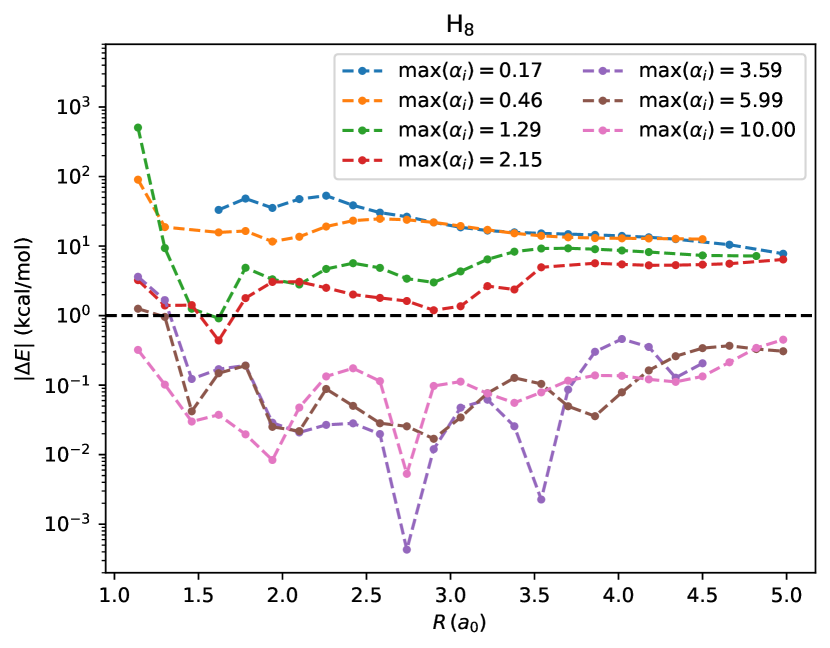
Figure 2: Energy errors along the H₈ potential energy curve for models with increasing non-local features. $R$ indicates the interatomic distance between H atoms.

III.1.2 Amount of training data

Ten models were trained on an increasing amount of data, from one geometry per chain to nine of them, to determine how the training-set size affects the validation performance. The effect of the training-set size on the validation error for several hydrogen chains is presented in Fig. 1c. In all cases, the models reached chemical accuracy for six training points, after which the error stabilised. This behaviour is mainly due to the fact that the model no longer has to extrapolate out of the range of $R$ values seen in the training set (the model is still validated on unseen values of $R$). This demonstrates a difference between the XC functional and non-interacting KEF. Li et al. Li et al. (2021) showed in their work that about two training points for each H₂ and H₄ are needed to accurately recover the potential energy curve, demonstrating great generalisation power. In contrast, training the non-interacting KEF is expected to require much more data.

The potential energy curves of the hydrogen chains are presented in Fig. 3 together with some selected densities, close to their respective minima and tending to dissociation. Both energies and densities have been obtained via an SCF calculation employing the trained functional.

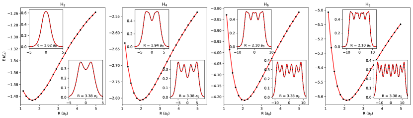
Figure 3: Potential energy curves of the hydrogen chains. Reference KS-DFT energies (black dots) and converged OF-DFT energies (red lines) are shown. The insets show the KS-DFT density in black compared to the converged OF-DFT density. The top insets show the density close to the minimum in the potential energy curve and bottom one the density for a geometry closer to dissociation. The $x$-axis of the inset represents the $x$-coordinate in atomic units and the $y$-axis the electron density ($n(x)$).

III.2 Non-interacting electrons

The next system is the one used by Snyder et al. Snyder et al. (2012) in their original work, which consists of a set of $N$ non-interacting, spinless electrons confined in a box, $x\in[0,1]$, feeling an external potential expressed as the sum of three Gaussian functions, generated by randomly sampling $a\in[1,10]$, $b\in[0.4,0.6]$ and $c\in[0.03,0.10]$:

$$v_{\text{ext}}(x)=\sum_{i=1}^{3}a\exp\left(-\frac{(x-b)^{2}}{2c^{2}}\right)$$ (20)

The Pauli functional is trained for different number of electrons, $N=2,\,3,\,4$, on a set of 100 random potentials. A final model is trained on 400 random potentials with $N\in[1,4]$. These models are validated on a different set of 1000 external potentials. The features fed to the MLP are:

$$z_{1} = n(x)$$ (21)

$$z_{i} = G[n](x;\alpha_{i}),\quad i>1$$ (22)

with the global convolution in Eq. (19). The validation energy and density errors are presented in Table 1. The density error is computed as:

$$(\Delta n)^{2}=\int_{0}^{1}\left(n(x)-n^{\prime}(x)\right)^{2}dx$$ (23)

where $n(x)$ and $n^{\prime}(x)$ are the reference KS-DFT and OF-DFT densities, respectively.

Table 1: Validation errors on a set of 1000 randomly generated external potentials for converged OF-DFT calculations with the trained Pauli functional. Energy errors in kcal/mol and density errors in $a_{0}^{-1}$.

$N$	$\overline{|\Delta E|}$	$|\Delta E|^{std}$	$|\Delta E|^{max}$	$\overline{\Delta n}$	$\Delta n^{std}$	$\Delta n^{max}$
2	0.10	0.15	2.51	$3.65\times 10^{-7}$	$2.33^{-6}$	$6.51\times 10^{-5}$
3	0.26	0.39	6.86	$2.00\times 10^{-6}$	$3.00^{-6}$	$3.70\times 10^{-5}$
4	0.48	0.72	8.10	$4.33\times 10^{-6}$	$8.60^{-6}$	$1.01\times 10^{-4}$
1—4	0.43	0.78	12.05	$3.71\times 10^{-6}$	$1.72^{-5}$	$3.17\times 10^{-4}$

Note that the errors in Table 1 are computed with the converged densities and energies from a regular SCF calculation since the Pauli potential becomes a smooth function of the density thanks to the gradient regularization. Fig. 4 shows the converged densities for several randomly selected external potentials with the number of electrons varying from 1 to 4. The Pauli potentials, computed from the converged OF densities, are presented in the bottom panels, showing a smooth behavior along the $x$ coordinate.

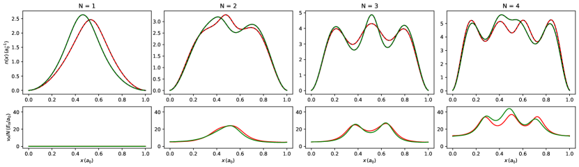
Figure 4: Top panels: samples of KS densities (black solid lines) and the corresponding converged OF densities (red and green dashed lines) for two randomly selected validation external potentials. Bottom panels: Pauli potentials for the converged densities.

III.3 Atoms

Finally, we validate our methodology for learning the KEF and XC functional on the atoms from the first two periods of the periodic table, extending the work from Ghasemi and Kühne Ghasemi and Kühne (2021) to a larger set of atoms and to the spin-polarized DFT framework. Atoms can be treated as an effective one-dimensional problem since only the radial part of the density has to be solved:

$$n(\mathbf{r})=n(r)n(\theta,\varphi),\quad n(\theta,\varphi)=1$$ (24)

Since we are considering multiple spin states, we will utilize the spin-polarized DFT in this scenario. The external and Coulomb potentialsOndřej Čertík (2010) are computed using the regular Coulomb interactions between charged particles:

$$v_{ext}(r) = -\frac{Z}{r}$$ (25)

$$v_{H}(r) = 4\pi\int_{0}^{\infty}\frac{n(r^{\prime})r^{\prime 2}}{|r-r^{\prime}|}dr^{\prime}$$ (26)

$$= 4\pi\left[\frac{1}{r}\int_{0}^{r}n(r^{\prime})r^{\prime 2}dr^{\prime}+\int_{r}^{\infty}n(r^{\prime})r^{\prime}dr^{\prime}\right]$$

Pauli and XC energies are computed as:

$$E_{F}[n^{\alpha},n^{\beta}]=4\pi\int_{0}^{\infty}f[n^{\alpha},n^{\beta}](r)n(r)r^{2}dr$$ (27)

where $f[n^{\alpha},n^{\beta}]$ is the Pauli or XC energy density.

For a spherically symmetric external potential the Schrödinger equation can be written as a one-dimensional equation,

$$\left[-\dfrac{1}{2}\dfrac{d^{2}}{dr^{2}}+\frac{l(l+1)}{2r^{2}}+v^{\sigma}(r)\right]u^{\sigma}(r)=\varepsilon^{\sigma}u^{\sigma}(r)$$ (28)

with $\psi^{\sigma}(r)=u^{\sigma}(r)/r$, $l$ the orbital angular momentum, and $v^{\sigma}(r)=v_{H}(r)+v^{\sigma}_{xc}(r)+[v^{\sigma}_{P}(r)]$, the latter potential term only present in OF-DFT. In OF-DFT case no centrifugal term is considered, that is $l=0$, since this is a kinetic-energy contribution which is described by the Pauli functional. The features fed to the MLP representing the functional energy density are:

$$z_{1} = \log(n^{\alpha}(r)+10^{-4})$$ (29)

$$z_{2} = \log(n^{\beta}(r)+10^{-4})$$ (30)

$$z_{i_{\alpha}} = G[n^{\alpha}](r;\alpha_{i_{\alpha}})$$ (31)

$$z_{i_{\beta}} = G[n^{\beta}](r;\alpha_{i_{\beta}})$$ (32)

where the convolution widths $\alpha_{i}$ are the same for $\alpha$ and $\beta$ densities and the convolution is computed as

$$G[n](r;\alpha)=\frac{1}{\sqrt{2\pi\alpha}}\int_{0}^{\infty}n(r^{\prime})\exp\left(-\frac{(r-r^{\prime})^{2}}{2\alpha}\right)dr^{\prime}$$ (33)

We demand that the XC energy density is always negative, so the output of the MLP is multiplied by $-1$ in this case. In order to make the energy density spin-symmetric, the same MLP is run twice and averaged for both spin orderings.

Similar to the previous test conducted on hydrogen chains, we evaluate the accuracy of Pauli and XC functionals with respect to the level of non-locality incorporated in the global features. In both cases the training set will consist of energies and densities of the elements in the first two periods of the periodic table. The reference energies and densities for the Pauli functional are computed with UKS/LDA. To learn the XC functional, the reference energies are computed with UCCSD(T)/cc-pVTZ using PySCFSun et al. (2018, 2020). UKS/LDA reference densities are taken in this case, similar to how DM21 was trained, leveraging the fact that the XC functionals are, in general, little sensitive to the reference densitiesKirkpatrick et al. (2021).

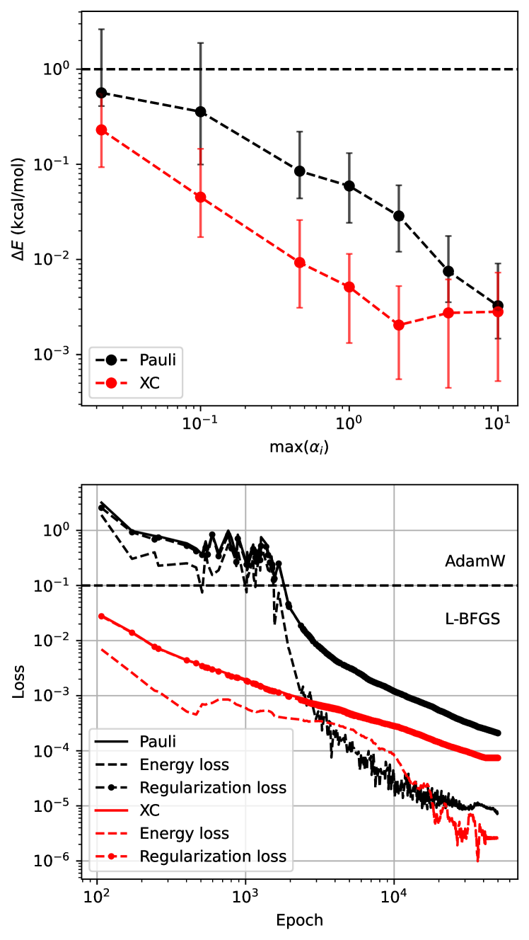
Figure 5: Comparison of the median errors of 10 training runs of the Pauli and XC functionals for the atoms in the first two periods of the periodic table against the amount of non-locality in the global features. The black points represent the average values of the median for all the atoms. Training loss curves for the largest model, together with the energy and regularization contributions, for the Pauli functional (black) and the XC functional (red).

The accuracy achieved by the Pauli and XC functionals with respect to the level of non-locality incorporated in the input features is compared in Fig. 5. While the XC functional needs little non-locality, reaching an excellent accuracy with only two narrow global convolutions, the Pauli functional does not produce accurate results until large convolutional widths are employed to construct the density features. The learning curves presented in the right panel of Fig. 5 already show a difference between both functional learning, where the Pauli functional needs a significantly larger amount of epochs to reach similar loss values than the XC functional. The regularization term is learned significantly faster for the XC functional, suggesting a less intricate structure of the underlying true functional, compared to the KEF.

The small amount of training data raises the question of how much of this precision is actually physics learned by the functional or pure overfitting. To answer this question we compute the ionization energies of the atoms with our learned functionals, since the cationic species were never seen in the training process. In Table 2 the ionization energies are presented for each atom compared to the reference energy in each case, i.e. KS-DFT/LDA energies to validate the Pauli functional and UCCSD(T) energies to validate the XC functional. These results present some clear overfitting in the case of Pauli functional, where in most cases it is not even possible to converge the SCF calculation of the cation, and those that converge present large energy differences. Although the learned XC functional is much more robust with respect to convergence, it also exhibits deviations from the actual ionization energies.

Table 2: Ionization energies of the atomic species in kcal/mol. For the learned functionals the energy difference (in kcal/mol) with respect to the reference ionization energy is presented.

Atom	KS-DFT/LDA-PW92	OF-DFT/Trained	$\tau_{max}=0.0$	$\tau_{max}=0.5$	$\tau_{max}=1.0$	$\tau_{max}=1.5$	CCSD(T)/cc-pVTZ	KS-DFT/Trained
He	560.16	$-0.02$	$-0.11$	$0.01$	$-0.01$	$-0.04$	565.58	$+6.21$
Li	125.40	$80.59$	$84.69$	$86.64$	$6.48$	$0.76$	123.44	$+25.24$
Be	208.11	$-$	$-1382.45$	$116.92$	$-0.86$	$-2.96$	214.11	$+25.61$
B	197.71	$+106.53$	$122.69$	$10.11$	$-0.67$	$0.55$	189.74	$+41.73$
C	271.25	$+141.81$	$166.88$	$61.14$	$5.98$	$-0.22$	257.92	$+50.29$
N	345.78	$+186.73$	$239.37$	$55.26$	$-$	$-0.95$	333.21	$+52.79$
O	320.51	$-$	$185.46$	$102.35$	$3.43$	$4.27$	307.29	$+50.58$
F	416.47	$+416.70$	$-$	$193.64$	$-1.80$	$-3.84$	395.30	$+58.68$
Ne	511.53	$+475.4$8	$-$	$434.67$	$9.52$	$-1.57$	491.41	$+60.11$

To test how the training of the Pauli functional would proceed in a more realistic scenario with a larger amount of training data, we generate larger datasets of atoms with fractional nuclear charges, under the external potential

$$v_{\text{ext}}(r)=-\frac{Z+\tau}{r}$$ (34)

where $\tau$ is a random number between $-0.1$ and $\tau_{\text{max}}$. Four datasets are generated with $\tau_{\text{max}}=0.0,\,0.5,\,1.0$, and $1.5$. The datasets contain a total number of 400 atoms with artificial nuclear charges, 40 samples per $Z$. The spin state is that for the ground of state of the atom with atomic number $Z$. In Table 2 the energy errors in the ionization energy are presented for each atom. The two datasets with larger $\tau_{\text{max}}$ provide much more information for the functional to gain physical insight about the true KEF. Note that these datasets do not necessarily contain the neutral and cation species, yet the functional becomes general enough as to accurately predict them.

IV Conclusions

In this work we present a new method to regularize the training of density functionals, derived from the variational condition that the global energy functional presents a minima for the ground electronic state density. In particular, the gradient of the Lagrangian with respect to the density is employed to guide the search of the functional which fulfills the minimum condition, making them applicable to regular SCF calculations. This methodology is directly applicable to the training of KEF and XC functional. This is a cheap regularization technique compared to performing a full SCF calculation for each of the training samples, and we anticipate that it can have widespread applicability in realistic functional training scenarios.

It is evident that forthcoming attempts to train the KEF will heavily depend on the inclusion of non-local features, which we have found to be more crucial than the number of global features and even the size of the network. The KEF reveals a more complex inner structure to learn, compared to the XC functional, as can be extracted from the regularization learning curves for both functionals with equivalent ML models and training schemes. Additionally, our findings reveal that the KEF is highly susceptible to overfitting on small datasets, as evidenced by its inability to accurately replicate the ionization energy of atoms. In contrast, the XC functional, which was solely trained on neutral atoms, displays remarkable robustness. Notably, all the SCF calculations converge to reasonable energies for the XC, while the KEF exhibits a dismal performance. Another instance where the KEF displays less generality than the XC is demonstrated in the hydrogen chain, where a greater number of training points was required for the KEF to accurately recover the potential energy curve compared to the XC case presented by Li et al. Therefore, it is anticipated that the datasets used to train the KEF must be substantially larger to enable the acquisition of sufficient physical knowledge. Alternatively, additional regularization techniques such as equipping the ML functional with exact scaling properties could be also used.

References

- Mardirossian and Head-Gordon (2017) N. Mardirossian and M. Head-Gordon, “Thirty years of density functional theory in computational chemistry: an overview and extensive assessment of 200 density functionals,” Molecular Physics 115, 2315–2372 (2017).
- Cramer and Truhlar (2009) C. J. Cramer and D. G. Truhlar, “Density functional theory for transition metals and transition metal chemistry,” Physical Chemistry Chemical Physics 11, 10757 (2009).
- Jain, Shin, and Persson (2016) A. Jain, Y. Shin, and K. A. Persson, “Computational predictions of energy materials using density functional theory,” Nature Reviews Materials 1 (2016).
- Hohenberg and Kohn (1964) P. Hohenberg and W. Kohn, “Inhomogeneous electron gas,” Physical Review 136, B864–B871 (1964).
- Kohn and Sham (1965) W. Kohn and L. J. Sham, “Self-consistent equations including exchange and correlation effects,” Physical Review 140, A1133–A1138 (1965).
- Wang and Carter (2002) Y. A. Wang and E. A. Carter, “Orbital-Free Kinetic-Energy Density Functional Theory,” in Theoretical Methods in Condensed Phase Chemistry, Progress in Theoretical Chemistry and Physics, Vol. 5, edited by S. D. Schwartz (Springer, 2002) pp. 117–184.
- Sears, Parr, and Dinur (1980) S. B. Sears, R. G. Parr, and U. Dinur, “On the Quantum-Mechanical Kinetic Energy as a Measure of the Information in a Distribution,” Israel Journal of Chemistry 19, 165–173 (1980).
- Deb and Ghosh (1983) B. M. Deb and S. K. Ghosh, “New method for the direct calculation of electron density in many-electron systems. I. Application to closed-shell atoms,” International Journal of Quantum Chemistry 23, 1–26 (1983).
- March (1986) N. March, “The local potential determining the square root of the ground-state electron density of atoms and molecules from the Schrödinger equation,” Physics Letters A 113, 476–478 (1986).
- Levy and Hui Ou-Yang (1988) M. Levy and Hui Ou-Yang, “Exact properties of the pauli potential for the square root of the electron density and the kinetic energy functional,” Physical Review A 38, 625–629 (1988).
- Perdew and Constantin (2007) J. P. Perdew and L. A. Constantin, “Laplacian-level density functionals for the kinetic energy density and exchange-correlation energy,” Phys. Rev. B 75, 155109 (2007).
- Francisco, Carmona-Espíndola, and Gázquez (2021) H. I. Francisco, J. Carmona-Espíndola, and J. L. Gázquez, “Analysis of the kinetic energy functional in the generalized gradient approximation,” The Journal of Chemical Physics 154, 084107 (2021).
- Chacón, Alvarellos, and Tarazona (1985) E. Chacón, J. E. Alvarellos, and P. Tarazona, “Nonlocal kinetic energy functional for nonhomogeneous electron systems,” Phys. Rev. B 32, 7868–7877 (1985).
- García-González, Alvarellos, and Chacón (1996) P. García-González, J. E. Alvarellos, and E. Chacón, “Nonlocal kinetic-energy-density functionals,” Physical Review B 53, 9509–9512 (1996).
- García-Aldea and Alvarellos (2008) D. García-Aldea and J. E. Alvarellos, “Fully nonlocal kinetic energy density functionals: A proposal and a general assessment for atomic systems,” The Journal of Chemical Physics 129, 074103 (2008).
- Sarcinella et al. (2021) F. Sarcinella, E. Fabiano, L. A. Constantin, and F. Della Sala, “Nonlocal kinetic energy functionals in real space using a Yukawa-potential kernel: Properties, linear response, and model functionals,” Physical Review B 103, 155127 (2021).
- Jumper et al. (2021) J. Jumper et al., “Highly accurate protein structure prediction with AlphaFold,” Nature 596, 583–589 (2021).
- Ravuri et al. (2021) S. Ravuri et al., “Skilful precipitation nowcasting using deep generative models of radar,” Nature 597, 672–677 (2021).
- Lin et al. (2023) Z. Lin, H. Akin, R. Rao, B. Hie, Z. Zhu, W. Lu, N. Smetanin, R. Verkuil, O. Kabeli, Y. Shmueli, A. dos Santos Costa, M. Fazel-Zarandi, T. Sercu, S. Candido, and A. Rives, “Evolutionary-scale prediction of atomic-level protein structure with a language model,” Science 379, 1123–1130 (2023).
- Degrave et al. (2022) J. Degrave et al., “Magnetic control of tokamak plasmas through deep reinforcement learning,” Nature 602, 414–419 (2022).
- Choo, Mezzacapo, and Carleo (2020) K. Choo, A. Mezzacapo, and G. Carleo, “Fermionic neural-network states for ab-initio electronic structure,” Nature Communications 11, 2368 (2020).
- Pfau et al. (2020) D. Pfau, J. S. Spencer, A. G. D. G. Matthews, and W. M. C. Foulkes, “Ab Initio solution of the many-electron Schrödinger equation with deep neural networks,” Physical Review Research 2, 033429 (2020).
- Hermann, Schätzle, and Noé (2020) J. Hermann, Z. Schätzle, and F. Noé, “Deep-neural-network solution of the electronic Schrödinger equation,” Nature Chemistry 12, 891–897 (2020).
- Dick and Fernandez-Serra (2020) S. Dick and M. Fernandez-Serra, “Machine learning accurate exchange and correlation functionals of the electronic density,” Nat. Commun. 11, 3509 (2020).
- Kirkpatrick et al. (2021) J. Kirkpatrick, B. McMorrow, D. H. P. Turban, A. L. Gaunt, J. S. Spencer, A. G. D. G. Matthews, A. Obika, L. Thiry, M. Fortunato, D. Pfau, L. R. Castellanos, S. Petersen, A. W. R. Nelson, P. Kohli, P. Mori-Sánchez, D. Hassabis, and A. J. Cohen, “Pushing the frontiers of density functionals by solving the fractional electron problem,” Science 374, 1385–1389 (2021).
- Kasim and Vinko (2021) M. Kasim and S. Vinko, “Learning the exchange-correlation functional from nature with fully differentiable density functional theory,” Physical Review Letters 127, 126403 (2021).
- Sun, Ruzsinszky, and Perdew (2015) J. Sun, A. Ruzsinszky, and J. P. Perdew, “Strongly Constrained and Appropriately Normed Semilocal Density Functional,” Physical Review Letters 115, 036402 (2015).
- Perdew (2001) J. P. Perdew, “Jacob’s ladder of density functional approximations for the exchange-correlation energy,” in AIP Conference Proceedings, Vol. 577 (AIP, Antwerp (Belgium), 2001) pp. 1–20.
- Medvedev et al. (2017) M. G. Medvedev, I. S. Bushmarinov, J. Sun, J. P. Perdew, and K. A. Lyssenko, “Density functional theory is straying from the path toward the exact functional,” Science 355, 49–52 (2017).
- Snyder et al. (2012) J. C. Snyder, M. Rupp, K. Hansen, K.-R. Müller, and K. Burke, “Finding density functionals with machine learning,” Physical Review Letters 108, 253002 (2012).
- Li et al. (2021) L. Li, S. Hoyer, R. Pederson, R. Sun, E. D. Cubuk, P. Riley, and K. Burke, “Kohn-sham equations as regularizer: Building prior knowledge into machine-learned physics,” Physical Review Letters 126, 036401 (2021).
- Helgaker et al. (2000) T. Helgaker, H. Larsen, J. Olsen, and P. Jørgensen, “Direct optimization of the AO density matrix in Hartree–Fock and Kohn–Sham theories,” Chemical Physics Letters 327, 397–403 (2000).
- Larsen et al. (2001) H. Larsen, J. Olsen, P. Jørgensen, and T. Helgaker, “Direct optimization of the atomic-orbital density matrix using the conjugate-gradient method with a multilevel preconditioner,” The Journal of Chemical Physics 115, 9685–9697 (2001).
- Jiang and Yang (2004) H. Jiang and W. Yang, “Conjugate-gradient optimization method for orbital-free density functional calculations,” The Journal of Chemical Physics 121, 2030–2036 (2004).
- Paszke et al. (2019) A. Paszke et al., “Pytorch: An imperative style, high-performance deep learning library,” in Advances in Neural Information Processing Systems 32 (Curran Associates, Inc., 2019) pp. 8024–8035.
- Snyder et al. (2013) J. C. Snyder, M. Rupp, K. Hansen, L. Blooston, K.-R. Müller, and K. Burke, “Orbital-free bond breaking via machine learning,” The Journal of Chemical Physics 139, 224104 (2013).
- Seino et al. (2018) J. Seino, R. Kageyama, M. Fujinami, Y. Ikabata, and H. Nakai, “Semi-local machine-learned kinetic energy density functional with third-order gradients of electron density,” The Journal of Chemical Physics 148, 241705 (2018).
- Ghasemi and Kühne (2021) S. A. Ghasemi and T. D. Kühne, “Artificial neural networks for the kinetic energy functional of non-interacting fermions,” The Journal of Chemical Physics 154, 074107 (2021).
- Kalita et al. (2021) B. Kalita, L. Li, R. J. McCarty, and K. Burke, “Learning to approximate density functionals,” Accounts of Chemical Research 54, 818–826 (2021).
- Imoto, Imada, and Oshiyama (2021) F. Imoto, M. Imada, and A. Oshiyama, “Order- n orbital-free density-functional calculations with machine learning of functional derivatives for semiconductors and metals,” Physical Review Research 3, 033198 (2021).
- Wu, Ren, and Zhao (2022) X. H. Wu, Z. X. Ren, and P. W. Zhao, “Nuclear energy density functionals from machine learning,” Physical Review C 105, L031303 (2022).
- Baker et al. (2015) T. E. Baker, E. M. Stoudenmire, L. O. Wagner, K. Burke, and S. R. White, “One-dimensional mimicking of electronic structure: The case for exponentials,” Physical Review B 91, 235141 (2015).
- Elliott et al. (2014) P. Elliott, A. Cangi, S. Pittalis, E. K. U. Gross, and K. Burke, “Almost exact exchange at almost no cost,” (2014).
- Ondřej Čertík (2010) Ondřej Čertík, “Theoretical physics,” (2010), https://www.theoretical-physics.com/dev/quantum/hf.html#hartree-potential-in-spherical-symmetry, accessed date 07.10.2022.
- Sun et al. (2018) Q. Sun, T. C. Berkelbach, N. S. Blunt, G. H. Booth, S. Guo, Z. Li, J. Liu, J. D. McClain, E. R. Sayfutyarova, S. Sharma, S. Wouters, and G. K.-L. Chan, “Pyscf: the python-based simulations of chemistry framework,” WIREs Computational Molecular Science 8, e1340 (2018).
- Sun et al. (2020) Q. Sun et al., “Recent developments in the pyscf program package,” The Journal of Chemical Physics 153, 024109 (2020).