Relational Event Modeling

Abstract

Advances in information technology have increased the availability of time-stamped relational data such as those produced by email exchanges or interaction through social media. Whereas the associated information flows could be aggregated into cross-sectional panels, the temporal ordering of the events frequently contains information that requires new models for the analysis of continuous-time interactions, subject to both endogenous and exogenous influences. The introduction of the Relational Event Model (REM) has been a major development that has led to further methodological improvements stimulated by new questions that REMs made possible. In this review, we track the intellectual history of the REM, define its core properties, and discuss why and how it has been considered useful in empirical research. We describe how the demands of novel applications have stimulated methodological, computational, and inferential advancements.

Keywords Endogenous effects  $\cdot$ longitudinal networks  $\cdot$ point processes  $\cdot$ relational events  $\cdot$ time-stamped interaction data

Introduction

Statistical models for social and other networks are receiving increased attention not only in specialized field journals such as Network Science or Social Networks, but also in prominent interdisciplinary science journals such as Science (Borgatti et al., 2009; Butts, 2009), PNAS (Stadtfeld et al., 2019), and Science Advances (Elmer and Stadtfeld, 2020).

Attention to statistical models for networks is on the rise also in well-established generalist statistics journals such as, for example, the Journal of the American Statistical Association (Hunter et al., 2008), the Journal of Applied Statistics (Snijders et al., 2010), Statistical Science (Schweinberger et al., 2020), and the Journals of the Royal Statistical Society (series A, B, and C) (Fienberg, 2012; Krivitsky and Handcock, 2014; Gile and Handcock, 2017; Vinciotti and Wit, 2017; Koskinen and Snijders, 2023). The Annual Review of Statistics and Its Applications itself has recently demonstrated considerable interest in models for social networks by publishing comprehensive and up-to-date reviews on two popular classes of statistical models: Exponential Random Graph Models (ERGMs) (Amati et al., 2018) and Stochastic Actor-Oriented Models (SAOMs) (Snijders, 2017).

Since the publication of these reviews, the increasing availability of time-stamped data resulting from innovation in data production, collection, storage and retrieval technologies has shown that network data samples collected at fixed time intervals are likely to miss fundamental differences in the time scales over which relational processes unfold (Golder et al., 2007). Computer-mediated communication (Lerner and Lomi, 2023), sociometric badges (Wu et al., 2008; Stehlé et al., 2011; Elmer and Stadtfeld, 2020), electronic trading platforms (Zappa and Vu, 2021), on-line interaction logs (Tonellato et al., 2023), and video recordings (Pallotti et al., 2022), are just some of the new data-generating technologies capable of producing large quantities of relational event data connecting sender and receiver units.

During the same period, studies based on event-oriented designs have become also increasingly common. While the empirical opportunities offered by relational event data have long been acknowledged by students of social networks (Freeman et al., 1987; Marsden, 1990; Borgatti et al., 2009), statistical models affording a degree of temporal resolution consistent with the frequency of observed social interaction (Butts, 2009) have become available only during the last fifteen years (Butts, 2008).

Time scales vary considerably based on interaction settings. High-frequency transactions in financial markets (Bianchi and Lomi, 2023) occur within seconds or fractions of seconds, while communication in emergency situations (Butts, 2008; Renshaw et al., 2023) may take several minutes. Email exchange (Perry and Wolfe, 2013) can extend over hours, whereas interaction generated by more complex forms of social coordination among corporate actors may become observable only over days or even weeks (Amati et al., 2019). In these various cases, aggregating time-stamped relational event data into network ties defined over conventional, or convenient, time periods, is unlikely to afford high fidelity representations of the underlying interaction processes (Tuma and Hannan, 1984).

Perhaps the main motivation that inspired the development of the Relational Event Model (REM) proposed by Butts (2008), was to provide a general analytical framework where sequential ordering and timing replace concurrency and temporal aggregation of network edges as the “dominant concepts of phenomenal concern” (Butts, 2008, p.192) in the analysis of social interaction. This involves deriving, specifying and estimating statistical models capable of assimilating and analyzing complex relational data without altering — through time aggregation — the natural time structure, and sequential ordering of observed social interaction. Conversation (Gibson, 2005), communication (Pilny et al., 2017), market exchange (Lomi and Bianchi, 2021), and other, more complex, forms of social coordination (Lerner and Lomi, 2020a) can be understood only with reference to the timing and sequential order of the relational events of interest (Abbott, 1992), which contain important information that is typically lost when time-stamped events are aggregated into binary network “ties” (Pallotti et al., 2022).

Since its introduction, the REM has been significantly refined and adapted to an ever-increasing diversity and sophistication of emerging empirical problems (Butts et al., 2023). This review piece provides an opportunity to position relational event modeling in the broader context of statistical models for network science, and assess the current state of field, incorporating a broad review of contemporary methodological, computational, and inferential developments in this class of statistical models for directed social interaction.

The paper is organized into eight main sections. Section 1 traces the intellectual origins and historical context of REMs. Section 2 identifies the observation plans and empirical research design elements typically associated with event-oriented studies of network dynamics. Section 3 surveys the available classes of REMs developed, at least in part, in response to specific problems with no satisfactory modeling solutions. Section 4 is dedicated to issues of empirical model specification and estimation. Section 5 examines the broad area of applications where REMs seem to have found fertile ground for development. Section 6 reviews the main challenges and open issues that orient current research. Section 7 concludes with a summary and a discussion of the main promises of relational event modeling.

1 Historical Context of Relational Event Models

Contemporary statistical models for social and other kind of networks rely heavily on the formalism of graph theory (Butts, 2009) — an inheritance left, in part, by earlier network models developed in sociometry (Moreno, 1934; Jennings, 1948), and within the structural tradition of social and cultural anthropology (White, 1963; Lévi-Strauss, 1971; Hage, 1979; Barnes and Harary, 1983; Hage and Harary, 1984). Concepts such as those of “degree,” “path distance,” “reciprocity,” and “transitive closure” that are central in contemporary statistical models for networks (Snijders, 2001; Amati et al., 2018) are firmly rooted in the mathematical representation of networks as graphs (Barabási, 2013).

The graph-theoretic formalism that inspired early Markov random graph models (Holland and Leinhardt, 1977, 1981; Frank and Strauss, 1986) may be considered to be the intellectual antecedent of contemporary statistical models for social networks (Wasserman and Pattison, 1996; Snijders, 2001; Snijders et al., 2006). It is only in relatively recent times that the limitations in representing networks of social relations as graphs have started to become apparent. REMs entail an alternative understanding of social relations as emergent from sequences of relational events connecting a sender behavioral unit to one or more receivers (Butts, 2008, 2009; Perry and Wolfe, 2013; Lerner and Lomi, 2023).

REMs provide a framework for analyzing and making inferences about the relational processes and dynamics in complex social systems. They are designed to capture the patterns of dependence in the occurrence and timing of relational events, such as communications, transactions, or social interactions, within a network.

Formally, REMs are rooted in event history models (see, e.g., Keiding, 2014, for a review), expressing the hazards of an event to occur, as a function of the history of previous events, as well as potentially additional nodal and relational attributes (Butts, 2008). REMs allow to study how events unfold over time, how they are influenced by various attributes and how they, in turn, affect the structure and evolution of the network.

The exact hazards of a REM may follow different functional forms and specifications. In many instances, the hazard is assumed to be piecewise constant, resulting in waiting times that are conditionally exponentially distributed. However, the precise definition of hazards will depend on the research questions and the empirical context, and these choices have implications for computational complexity, model fit, and the interpretation of the model (Butts and Marcum, 2017; Schaefer and Marcum, 2017; Stadtfeld et al., 2017).

Two other modeling frameworks are appropriate for the analysis of longitudinal networks, the temporal ERGM and the SOAM. The formulation of the ERGM (Robins et al., 2007) may be understood in terms of the conditional probability of a network edge, given the relationships among all other network edges (Wasserman and Pattison, 1996; Snijders et al., 2006). In the ERGM the edges connecting pairs of senders and receivers are assumed to be interdependent, and such interdependencies can be captured by local configurations of network ties such as triangles or star-shaped structures (Robins et al., 2007). More specifically, the existence of a tie in a social network is conditionally independent of ties that are far distant in space (Frank and Strauss, 1986). Temporal extensions of the ERGM (Hanneke et al., 2010; Krivitsky and Handcock, 2014) have been introduced to model network dynamics over time.

The SAOM (Snijders, 1996, 2001, 2005, 2017), is a probability model evaluating change in network ties (relational states) observed in adjacent time periods. While the SAOM takes into account relational states observed at multiple time points, it operates under the assumption that ties change continuously over time through a series of micro-steps occurring between observations. Each micro-step involves at most one alteration (Holland and Leinhardt, 1977) in the network with social actors choosing what ties to alter based on a multinomial choice probability model (McFadden, 1973) accounting for the local configurations in which potential ties are embedded.

2 Relational Data and Study Design

The relational event modeling framework has been introduced to analyze the dynamics underlying social networks, with a focus on understanding the complex interactions and dependencies between behavioral units over time. REMs are flexible because they integrate temporal, structural, and attributional aspects of the data within a single framework. This flexibility sustains specification of very general, yet detailed models of network evolution (Brandes et al., 2009).

2.1 Network Structure

The building block of the REM is the relational event, defined as an interaction initiated by a sender unit and directed toward one or more targets (Butts, 2008). Examples include hospitals sharing patients (Vu et al., 2017; Amati et al., 2019), credit institutions exchanging financial assets (Lomi and Bianchi, 2021; Zappa and Vu, 2021; Bianchi and Lomi, 2023), students telephoning each other (Stadtfeld and Block, 2017), people interacting face-to-face (Elmer and Stadtfeld, 2020) and in social groups (Hoffman et al., 2020), or employees exchanging emails (Quintane et al., 2013; Perry and Wolfe, 2013).

REMs can also model relations between units belonging to different classes in the context of more general bipartite processes. Examples include non native species invading new spatial niches (Juozaitienė et al., 2023), editors modifying Wikipedia pages (Lerner and Lomi, 2017), computer developers fixing software problems (Tonellato et al., 2023), and political actors supporting or rejecting proposed legislation (Brandenberger, 2018b; Haunss and Hollway, 2022).

Although relational events are typically defined between a single sender and a single receiver, generalizations are possible where a sender may reach multiple receivers simultaneously. This situation is common in technology-mediated communication (Lerner and Lomi, 2023), citation networks (Lerner and Hâncean, 2023; Filippi-Mazzola and Wit, 2023), and social gatherings attended by many participants (Lerner et al., 2021).

2.2 Sampling and Recording

Event network studies typically look at social units interacting within a bounded environment. Examples of geographical areas consist of student houses (Stadtfeld and Block, 2017) or hospitals within geographical regions (Vu et al., 2017; Zachrison et al., 2022), whereas examples of temporal boundaries involve interaction between emergency teams during different phases of a crisis (Butts, 2008), or hospitals transferring patients in specific days of the week (Amati et al., 2019). Relational events taking place outside the main observation domain are usually not recorded, so the social networks reconstructed from streams of relational events are often incomplete. Unlike studies of statistically independent observations, network boundary specification might affect the validity, robustness, and replicability of the results (Laumann et al., 1989).

3 Specifications of Relational Event Models

The units of analysis in the REM are the edges connecting individual pairs of senders and receivers. Those edges are typically stored in tuples $(t,s,r)$, where $s$ is the sender, $r$ is the receiver, and $t$ is the time of the relational event connecting $s$ to $r$. At its core, the REM is defined as a point process for directed pairwise interactions that, in turn, are modeled through their rate function $\lambda$. The model assumes that $\lambda$ may depend upon sender, receiver, past event history, and/or exogenous covariates.

Notation

Notation	Meaning
$(t,s,r)$	A relational event in which sender $s$ interacts with receiver $r$ at time $t$
$\lambda_{sr}(t)$	Rate/hazard at which sender $s$ contacts receiver $r$ at time $t$
$\mathcal{H}_{t}$	Filtration of the process, containing all information about relational events until time $t$
$L,L_{P}$	Likelihood and partial likelihood
$\mathcal{R}(t)$	Risk set at time $t$, consisting of all relational events that can happen at that time
$\widetilde{\mathcal{R}}(t)$	Sampled risk set at time $t$, consisting of the event $(s,r)$ at time $t$ and a set of sampled non-events
$x_{sr}(t)$	Dyadic covariate(s) with corresponding effect(s) $\beta$
$z_{sr}(t)$	Dyadic covariate(s) with corresponding random effect(s) $\gamma$
$a$	Alter, i.e., an individual different from sender or receiver

3.1 Types of Relational Event Models

We consider a fixed time interval $[0,T]$, with $0<T<\infty$, in which events occur. Events are defined as time-stamped interactions between senders and receivers. Both the set of senders $\mathbf{S}$ and receivers $\mathbf{R}$ are assumed to be finite. For one-mode networks the set of senders and receivers overlap, $\mathbf{S}=\mathbf{R}$, whereas for two-mode or bipartite networks they are distinct. The relational event process is a marked point process (Daley and Vere-Jones, 2003; Cressie, 2015) based on more general approaches (Borgan et al., 1995; Aalen et al., 2008) for event history sequences $\left\{(t_{i},s_{i},r_{i}):~{}i\geq 1,s_{i}\subset\mathbf{S},r_{i}\subset\mathbf{R}\right\}$, and defined on a probability space $(\Omega,\mathcal{F},P)$ adapted to the filtration $\mathcal{H}_{t}$, consisting of the history of process (Andersen et al., 1993). In principle, the marks $(s,r)$ can be individuals or sets of senders and receivers.

Associated with this marked point process, we define a multivariate counting process $N$, whose components $N_{sr}$ record the number of directed interactions between $s$ and $r$,

$$N_{sr}(t)=\sum_{i\geq 1}\mathbbm{1}_{\left\{t_{i}\leq t;~{}s_{i}=s;~{}r_{i}=r\right\}}.$$

According to the Doob–Meyer decomposition theorem (Meyer, 1962), there exists a predictable process $\Lambda_{sr}$ and a residual martingale process $M_{sr}$, such that the counting process can be written as

$$N_{sr}(t)=\Lambda_{sr}(t)+M_{sr}(t).$$

The aim of the REM is to describe the structure of the predictable cumulative hazard process $\Lambda_{sr}$. By assuming that the counting process is an inhomogeneous Poisson process, we can write the cumulative hazard as

$$\Lambda_{sr}(t)=\int_{0}^{t}\lambda_{sr}(\tau)~{}d\tau,$$

where $\lambda_{sr}$ is the hazard function of the relational event $(s,r)$. The general REM is defined as

$$\lambda_{sr}(t)=\mathbbm{1}_{\{(s,r)\in\mathcal{R}(t)\}}\>\lambda_{0}(t)\>\psi\Bigl{\{}\beta(t),x_{sr}(t)\Bigr{\}},$$ (1)

where $\lambda_{sr}(t)$ is only non-zero if the event $(s,r)$ is contained in the risk set $\mathcal{R}(t)$ of possible events at time $t$, $\lambda_{0}(t)$ is the baseline hazard function unrelated to $(s,r)$, $\psi$ is a relative risk function as defined in Thomas (1981), $x_{sr}(t)$ is the $\mathcal{H}_{t}$ measurable set of endogenous and exogenous (possibly) time-varying variables, and $\beta(t)$ are the effect sizes. The function $\psi$ is positive and, for identifiability, normalized by setting $\psi(\beta,0)=1$.

The relational event literature has focused on the exponential risk function $\psi(\beta,x)=\exp(\beta^{\top}x)$. Under the conditional independence framework (Besag, 1974, 1975), network statistics are, by construction, dependent through space and time. Accordingly, the propensity of pairs of senders and receivers to mutually connect depends on which relational events they have sent or received in the past, their order in time, if not their exact timing, and on exogenous factors like nodal or network attributes.

3.1.1 The Original Relational Event Model

Butts (2008) introduced the REM as a piece-wise homogeneous Poisson process, whereby the rate function was specified as

$$\lambda_{sr}(t)=\lambda_{0}\>\exp\Bigl{\{}\beta^{\top}x_{sr}(t)\Bigr{\}}\mathbbm{1}_{\left\{(s,r)\in\mathcal{R}(t)\right\}},$$ (2)

where $x_{sr}(t)$ is the collection of sufficient network statistics associated with the parameter vector $\beta\in\mathbb{R}^{p}$. The covariates in $x_{sr}(t)$ can depend on nodal characteristics, such as the age of $r$ or the age difference between the pair $(s,r)$, and also on the history of the process. For instance, the covariates $x_{sr}(t)$ can include a count of the number of past events between $(s,r)$ before time $t$.

In the original formulation, the baseline rate of the interaction process $\lambda_{0}$ is assumed constant. This means that the waiting times between events is exponentially distributed, and once an event takes place, the context of the action is changed, and all the possible relational event waiting times are restarted.

3.1.2 Weighted and Signed Networks

One of the first extensions of the original REM involved geopolitical conflicts and cooperation (Brandes et al., 2009). The authors highlighted that each interaction event between countries, international organizations, or ethnic groups could be given either a positive or negative weight according to the degree of cooperation or hostility between countries.

In this extended relational event definition $(t,s,r,w)$, the interaction weight $w$ is modeled alongside the event $(t,s,r)$ as $p\left\{(t,s,r,w)~{}|~{}\mathcal{H}_{t-}\right\}=p\left\{(t,s,r)~{}|~{}\mathcal{H}_{t-}\right\}\times p\left\{w~{}|~{}(t,s,r),\mathcal{H}_{t-}\right\}$. The second term models the interaction weights depending on which countries are interacting and how they interacted in the past, whereas the first term is the usual REM likelihood, which is also allowed to depend on past interaction weights included in $\mathcal{H}_{t-}$.

Subsequent versions of the REM have accommodated weighted network statistics (Amati et al., 2019; Bianchi and Lomi, 2023) associating a decay function $f\left(t,t_{i},\alpha\right)$ to each past event $(s_{i},r_{i})$ where $t$ is the current time, and $\alpha$ a decay parameter. In its simplest formulation, the temporal relevance of an event is assumed to decrease according to a power law, $f\left(t,t_{i},\alpha\right)=\left(t-t_{i}\right)^{-\alpha}$, though other specifications may be used instead (Lerner and Lomi, 2020b).

3.1.3 Multicast or Polyadic Interaction

Multicast (or “polyadic”) interaction occurs when a single event links an individual sender to multiple receivers simultaneously. The possibility of one-to-many interaction was explicitly recognized by DuBois et al. (2013) in their model of teacher-students interaction in a classroom context. In the same year, Perry and Wolfe (2013) provided a more general formulation specification of the intensity function for a sender $s\in\mathbf{S}$ addressing a set of receivers $R=\{r_{1},\dots,r_{m}\}\subset\mathbf{R}$, taking

$$\lambda_{sR}(t)=\lambda_{0s}(t;\lvert R\rvert)\>\exp\left\{\beta_{0}^{\top}\sum_{r\in\mathcal{R}_{s}(t)}x_{sr}\left(t\right)\right\}\prod_{r\in R}\mathbbm{1}_{\left\{r\in R_{s}(t)\right\}}.$$ (3)

The event rate function involves two types of stratification, discussed in greater detail in Sections 3.1.4 and 3.2.3, which explains the sender-specific definition of the risk set $\mathcal{R}_{s}(t)$ and baseline hazard, which also depend on the size of the receiver set. The network statistics are defined as the sums of the individual dyadic statistics $x_{sR}(t)=\sum_{r\in R}x_{sr}(t)$.

Lerner and Lomi (2023) introduced the Relational Hyperevent Model (RHEM) by generalizing the definition of multicast network statistic. A hyperedge covariate $x_{sR}$ is a function of the sender and the entire set of receivers that cannot, necessarily, be decomposed into the sum of dyadic covariates. An example of hyperedge covariate is inertia, the tendency toward repeating past relational events, defined as

$$x_{sR}^{\mbox{inertia}}(t)=\sum_{t_{i}<t}f(t,t_{i},\alpha)\mathbbm{1}_{\left\{s_{i}=s,R_{i}=R\right\}}.$$

In email exchange, for instance, the existence of a mailing list may result in a moderator communicating with exactly the same group of individuals. Instead, unordered repetition captures interaction within a stable set of actors with turn-taking among the senders (Gibson, 2005). Replacing dyadic covariates with their hyperedge counterparts not only provides a richer collection of network effects but also improves model fit (Lerner and Lomi, 2023).

Alternative approaches for modeling polyadic interactions have been proposed. Kim et al. (2018) introduced the Hyperedge Event Model, assuming that dyadic intensities stochastically determine the sender of the next event and its receiver set. Mulder and Hoff (2021) introduced a latent variable model whereby all potential receivers are assigned to the receiver set on the basis of a suitability score depending on the sender and receiver-specific characteristics.

3.1.4 Separable Intensity Functions

Stadtfeld et al. (2017) developed the Dynamic Network Actor Model (DyNAM), an actor-oriented model for relational event data built upon the same paradigm introduced by Snijders (1996, 2017). The distinctive feature of the DyNAM is that it explains social interaction in terms of “individuals’ preferences, available interaction opportunities, and individuals’ perception of the social network they are embedded in” (Stadtfeld and Block, 2017, p.318). Accordingly, the inferential framework of the DyNAM consists of modeling a composite process made of (i) the sender’s decision to initiate a relational event at a certain point in time, and (ii) the sender’s decision to address a specific receiver. The DyNAM decomposes event rates into two, sender-centred, components, i.e.,

$$\lambda_{sr}(t)=\underbrace{\lambda_{s}(t)}_{\text{select sender $s$}}\times\underbrace{p\left(r\mid s\right)}_{\text{\parbox{71.13188pt}{\centering sender $s$ \\ addresses~{}receiver~{}$r$\@add@centering} }}.$$ (4)

Similar to Snijders (2005), senders’ event rates rates $\lambda_{s}$ are modeled through an exponential link function evaluating nodal attributes at individual and network levels,

$$\lambda_{s}(t)=\lambda_{0}\exp\,\left(\theta^{\top}x_{s}\right)\mathbbm{1}_{\left\{s\in\mathcal{R}(t)\right\}}.$$ (5)

Following McFadden (1973), receiver choice is modeled via a multinomial distribution, i.e.,

$$p\left(r\mid s,\mathcal{H}_{t}\right)=\genfrac{}{}{}{}{\raisebox{3.0pt}{$\exp\left\{\beta^{\top}x_{sr}(t)\right\}$}}{\raisebox{-3.0pt}{$\sum_{r^{\prime}\in\mathcal{R}_{s}(t)}\exp\left\{\beta^{\top}x_{sr^{\prime}}(t)\right\}$}}.$$ (6)

The timing distribution does not explicitly depend on the receiver characteristics and this typically sacrifices model fit over an actor-oriented interpretation of the model parameters.

The DyNAM has recently been extended with the incorporation of the DyNAM-i (Hoffman et al., 2020), which explains sequences of joining and leaving events in the context of group-based interactions. This extension captures (i) the specific nature of group conversations and interactions that typically occur in cliques; and (ii) the need to align network modeling strategies with the increasing use of sensor technologies, such as Bluetooth or RFID badges, to detect collective interaction.

Vu et al. (2017) exploited the separability of intensity functions by decomposing the stream of relational events into event times and event destinations. The separable sender intensity and receiver choice model adds more flexibility to the relational event framework allowing for the separation between senders and receiver effects, and not only between event weights and dyads as in Brandes et al. (2009).

3.2 Network Covariates

Given the general expression of the REM hazard in Eq. 1, the drivers of the relational process $x_{st}(t)$ describe known, $\mathcal{H}_{t-}$ measurable, quantities quantifying endogenous or exogenous statistics of the sender, the receiver or both.

3.2.1 Endogenous VS Exogenous Covariates

In statistical models for networks (e.g., Snijders et al., 2010), covariates are endogenous to the extent that they depend on past interaction. Covariates are exogenous when they depend on characteristic of single nodes (monadic covariates) or pairs or nodes (dyadic covariates). One example of endogenous covariate is reciprocity, while gender and geographical distance are exogenous covariates, representing monadic and dyadic characteristics, respectively. A basic selection of endogenous and exogenous covariates is displayed in Table 1. Other ad-hoc specifications, such as those based on exchange sequences in conversational analysis, are explained in Butts (2008).

Table 1: Basic menu of network covariates defined in the REM

Network Covariate Mechanism Formula Out-degree $\displaystyle\sum\limits_{a\neq s}N_{sa}(t^{-})$ Out-intensity $\genfrac{}{}{}{}{\raisebox{3.0pt}{$1$}}{\raisebox{-3.0pt}{$\text{out-degree}_{s}(t)$}}\displaystyle\sum\limits_{a\neq s}\displaystyle\sum\limits_{i:~{}s_{i}=s,r_{i}=a}f\Big{(}t,t_{i},\alpha\Big{)}$ In-degree $\displaystyle\sum\limits_{a\neq s}N_{as}(t^{-})$ In-intensity $\genfrac{}{}{}{}{\raisebox{3.0pt}{$1$}}{\raisebox{-3.0pt}{$\text{in-degree}_{s}(t)$}}\displaystyle\sum\limits_{a\neq s}\displaystyle\sum\limits_{i:~{}s_{i}=a,r_{i}=s}f\Big{(}t,t_{i},\alpha\Big{)}$ Repetition $N_{sr}(t^{-})$ Reciprocation $N_{rs}(t^{-})$ Transitive closure $\displaystyle\sum\limits_{a\neq s,r}N_{sa}(t^{-})N_{ra}(t^{-})$ Cyclic closure $\displaystyle\sum\limits_{a\neq s,r}N_{as}(t^{-})N_{ra}(t^{-})$ Sending balance $\displaystyle\sum\limits_{a\neq s,r}N_{sa}(t^{-})N_{ra}(t^{-})$ Receiving balance $\displaystyle\sum\limits_{a\neq s,r}N_{as}(t^{-})N_{ar}(t^{-})$ Node attribute $x_{sr}(t)$ Node matching $\text{dist}\left\{x_{s}(t)=x_{r}(t)\right\}$ Notes. (Out/in)-(degree/intensity) statistics can refer to both senders and receivers. Node $a$ is a third (alter) trading counterpart of the sender-receiver pair $(s,r)$. The term $N_{sr}(t^{-})$ is the number of relational events flowing from sender $s$ to receiver $r$ right before time $t$, while $f(t,t_{i},\alpha)=(t-t_{i})^{-\alpha}$ is the decay function accounting for the temporal relevance of previous relational events. In depicting network statistics, solid line arrows ($\rightarrow$) refer to past relational events, while dashed arrows ($\dashrightarrow$) indicate current relational events.

An additional consideration refers to the hierarchy principle, whereby lower-order interaction terms should always be included in the presence of higher-order interaction terms (Pattison and Robins, 2002; Wang et al., 2013). In the REM, for example, failing to account for heterogeneity of the senders and receivers may result in incorrect detection of triadic effects (Juozaitienė and Wit, 2022a).

3.2.2 Heterogeneity

There are two fundamental types of heterogeneity in event networks. Endogenous heterogeneity, or emergence, refers to the inherent stochasticity of the process itself combined with the dependence of future interactions on current ones. An example is virality, whereby, for instance, a paper gets cited because it was cited many times before. In the REM, endogenous heterogeneity can be captured by endogenous covariates.

The second type of heterogeneity, extrinsic variation, is either observed, such as the prestige of the institutions of the authors of a paper, or latent, such as the quality of the work it represents. Latent extrinsic heterogeneity in the REM can be expressed by means of random effects. Juozaitienė and Wit (2022a) and Uzaheta et al. (2023) proposed mixed effect extensions of the REM, i.e.,

$$\lambda_{sr}(t)=\mathbbm{1}_{\{(s,r)\in\mathcal{R}(t)\}}\>\lambda_{0}(t)\>\exp\left\{\beta^{\top}x_{sr}(t)+\gamma^{\top}z_{sr}(t)\right\},$$

with dyadic covariates $z_{rs}(t)$ and $\gamma\sim N(0,\Sigma)$ the random effects. Estimation of the random effects variance can be done via Expectation Maximization (Dempster et al., 1977) or Laplace approximations of the likelihood (Pinheiro and Bates, 2006), or in certain cases via a penalized zero order spline approach (Wood, 2017).

DuBois et al. (2013) suggested a model that accounted for sender and receiver heterogeneity by means of a stochastic block structure. More recently, in an analysis of a communication network Juozaitienė and Wit (2022a) showed that incorporating random effects for both the sender and receiver enhances the model fit compared to model specifications that solely rely on endogenous degree-based statistics. Therefore, the inherent differences between individuals in the network drives part of the heterogeneity in the interactions.

3.2.3 Stratification

Conceptually, stratification can be introduced either to model event streams in multiplex networks or to account for heterogeneity by specifying different baseline intensity functions for individual sets of dyads. Perry and Wolfe (2013); Bianchi and Lomi (2023), for example, use sender-based stratification, effectively allowing each sender to have its own individual baseline hazard, i.e.,

$$\lambda_{sr}(t)=\lambda_{0s}(t)\exp\left\{\beta_{0}^{\top}x_{sr}(t)\right\}\mathbbm{1}_{\left\{(s,r)\in\mathcal{R}(t)\right\}}.$$

Receiver-based stratification is defined in a similar fashion, and usually occurs when there is heterogeneity in those nodes that are repeatedly targeted as receivers. In citation networks, for example, groundbreaking articles or patents have very distinct, individual citation profiles, which makes a receiver-based baseline hazards an attractive option, given that they not have to be estimated individually (Filippi-Mazzola and Wit, 2023).

Juozaitienė and Wit (2022b) proposed a stratified version of the REM, in which distinct baseline hazards are associated with distinct families of temporal network effects, such as reciprocity in its direct and generalized forms. Subsequent baseline hazard estimation reveals the tendency of some endogenous covariates to have very specific temporal effect-profiles.

4 Estimation and Computation

The fundamental information about a sequence of relational events $\{(t_{i},s_{i},r_{i}):i=1,\ldots,n\}$ is contained in its likelihood function. For a REM, this function can be expressed as the product of the conditional generalized exponential event time densities and their associated multinomial relational event probabilities, i.e.,

$$L(\beta)=\prod_{i=1}^{n}\sum_{(s,r)\in\mathcal{R}(t_{i})}\lambda_{sr}(t_{i})\exp\left\{-\sum_{(s,r)\in\mathcal{R}(t_{i})}\int_{t_{i-1}}^{t_{i}}\lambda_{sr}(\tau)d\tau\right\}\genfrac{}{}{}{}{\raisebox{3.0pt}{$\lambda_{s_{i}r_{i}}(t_{i})$}}{\raisebox{-3.0pt}{$\sum_{(s,r)\in\mathcal{R}(t_{i})}\lambda_{sr}(t_{i})$}},$$ (7)

where $\lambda$ is a function of $\beta$ and $\mathcal{R}(t)$ is the risk set, i.e., the set of all possible events that could have occurred at time $t$.

Estimating the parameters of REMs by maximizing the full likelihood poses several challenges. The likelihood function is indeed a complex object that involves explicit integration across the unknown hazard function and sums over large risk sets. In this section, we will explore computational alternatives proposed to overcome the complexity of the full likelihood approach.

4.1 Partial Likelihood Estimation

The proportional hazard model (Cox and Oakes, 1984) offers an attractive alternative to fully parametric models due to its absence of distributional assumptions regarding activity rates, which are then treated as nuisance parameters. It offers an effective simplification of the full REM likelihood through the application of the partial likelihood $L_{P}$ (Cox, 1975) to counting processes (Andersen and Gill, 1982) on network edges, which only involves multinomial event probabilities, i.e.,

$$L_{P}(\bm{\beta})=\prod_{i=1}^{n}\left(\genfrac{}{}{}{}{\raisebox{3.0pt}{$\exp\left\{\beta^{\top}x_{s_{i}r_{i}}(t_{i})\right\}$}}{\raisebox{-3.0pt}{$\sum_{(s,r)\in\mathcal{R}(t_{i})}\exp{\left\{\beta^{\top}x_{sr}(t_{i})\right\}}$}}\right).$$ (8)

This expression eliminates the unknown baseline hazard, resulting in a more adaptive representation of the underlying network dynamics, while being able to estimate the parameters in a straightforward way by maximizing $L_{P}(\beta)$. An example is given in Figure 1.

As Butts (2008) noted, the partial likelihood corresponds to the full likelihood when only the event orderings are known, but not the exact timings. However, the partial likelihood approach faces a limitation in large networks, as the risk set in its denominator tends to expand quadratically with the number of nodes.

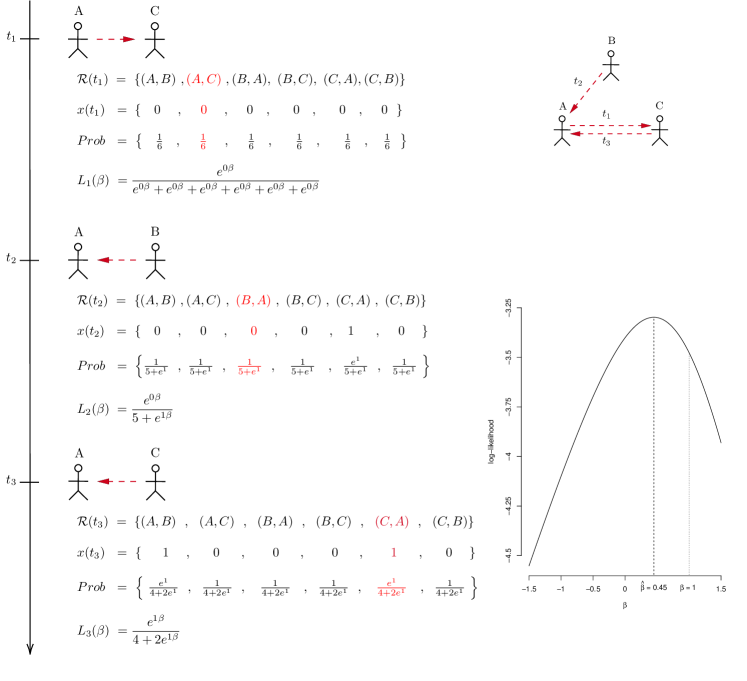
Figure 1: Example of a relational event process among three subjects $\{A,B,C\}$ based on the hazard function $\lambda_{sr}(t_{i})=\lambda_{0}(t_{i})\exp\left\{\beta x(t_{i})\right\}$, with $\beta=1$, whereby the event rate is influenced by the reciprocation statistic $x(t_{i})$. The left-hand side of the figure outlines the unfolding of the sequence of relational events according to the true probabilities Prob, mirrored in the graphical representation in the upper right. At each time point, the risk set $\mathcal{R}(t)$ consists of all six possible interactions between pairs of individuals. At time $t_{1}$, an interaction from $A$ to $C$ is observed, while all reciprocation covariates are zero, as no interaction has occurred yet. The probability of each event is determined using Eq. 8, with partial likelihood $L_{1}(\beta)$. At time $t_{2}$, an interaction from $B$ to $A$ occurs. This event has partial likelihood $L_{2}(\beta)$, with one reciprocal non-event in the denominator. At $t_{3}$, the reciprocal interaction from $C$ to $A$ is observed, with partial likelihood $L_{3}(\beta)$. The overall partial likelihood $L_{P}(\beta)=\prod_{i=1}^{3}L_{i}(\beta)$ is maximized at $\hat{\beta}=0.45$, as shown in the lower-right side of the figure, close to the actual effect size $\beta=1$.

4.1.1 Risk Set Sampling

The primary constraints in modeling the partial likelihood from Eq. 8 are found in the risk set size. The idea of adopting subsampling strategies to approximate the partial likelihood was noted by Butts (2008). Vu et al. (2015) initially introduced a, more efficient, nested-case control sampling strategy (Borgan and Keogh, 2015) to mitigate the computational complexity involved in estimating the partial likelihood.

Nested case-control sampling consists of sampling from the current risk set $\mathcal{R}(t)$ according to some probability $\pi\{\cdot\mid\mathcal{R}(t)\}$ a set of non-events, or controls, for each event, or case. The sampled non-events together with the events are called the sampled risk set $\widetilde{\mathcal{R}}(t)$. Borgan et al. (1995) show that the sampled partial likelihood $\widetilde{L}_{P}$, accounting for the sampling probabilities is a valid likelihood. When this probability is assumed to be random, i.e., $\pi\{\cdot\mid\mathcal{R}(t)\}=1/|\mathcal{R}(t)-1|$, $\widetilde{L}_{P}(\beta)$ reduces to the simplified form, i.e.,

$$\widetilde{L}_{P}(\bm{\beta}) =\prod_{i=1}^{n}\left(\genfrac{}{}{}{}{\raisebox{3.0pt}{$\pi((s_{i},r_{i})|\mathcal{R}(t_{i}))\exp\{{\beta^{\top}x_{s_{i}r_{i}}(t_{i})\}}$}}{\raisebox{-3.0pt}{$\sum_{(s,r)\in\widetilde{\mathcal{R}}(t)}\pi((s,r)\mid\mathcal{R}(t_{i}))\exp{\{\beta^{\top}x_{sr}(t_{i})\}}$}}\right)$$

$$=\prod_{i=1}^{n}\left(\genfrac{}{}{}{}{\raisebox{3.0pt}{$\exp\{{\beta^{\top}x_{s_{i}r_{i}}(t_{i})\}}$}}{\raisebox{-3.0pt}{$\sum_{(s,r)\in\widetilde{\mathcal{R}}(t)}\exp{\{\beta^{\top}x_{sr}(t_{i})\}}$}}\right),$$ (9)

where $\widetilde{\mathcal{R}}(t)$ is the sampled risk set.

Lerner and Lomi (2020b) employed nested case-control sampling to empirically showcase the efficiency of estimates on large networks, even when a limited number of non-events is sampled.

4.1.2 Computational Aspects of Stratified Relational Event Models

Perry and Wolfe (2013) proposed the first REM that introduced sender stratification to expedite calculations and combined it with a customized method for maximizing the log partial likelihood. Vu et al. (2015) proposed a flexible stratification methods allowing for data structures with many types of nodes and events, then showing the scalability of their approach to large data sets. Combining the two approaches, Bianchi and Lomi (2023) proposed a sender-stratified REM for high-frequency data, using nested case-control sampling to update the risk set at each new event. This model specification has been tested in empirical applications using millions of financial transactions. Filippi-Mazzola and Wit (2023) proposed a receiver-stratified REM for the analysis of millions of patent citations, in which the hazard is modeled via smooth functions of the covariates using a spline approach.

4.2 Baseline Hazard Estimation

With the advancement of REMs, the prevailing method for their estimation is based on the partial likelihood method (Cox, 1975), which treats the baseline hazard as a nuisance parameter. However, gaining insights into the temporal variations of the underlying event rates can be valuable for visualizing the baseline hazard.

Two common approaches to estimate the baseline hazard are the Breslow estimator (Breslow, 1972) and the Nelson–Aalen estimator (Nelson, 1972; Aalen, 1978). Both estimate the cumulative hazard function only at the observed event times, and so does not capture the continuous nature of the underlying baseline hazard function. Meijerink-Bosman et al. (2022) estimated the baseline hazard by assuming fixed baseline hazard rates within expanding windows. Juozaitienė and Wit (2022a) and Juozaitienė et al. (2023) improved smooth baseline hazard recovery by a spline-based approximation.

4.3 Model Comparison and Diagnostic Tools

Traditional approaches, such as likelihood ratio tests, Akaike Information Criterion (AIC), and Bayesian Information Criterion (BIC), are widely adopted for comparing REMs (Foucault Welles et al., 2014; Pilny et al., 2016). Whereas model comparison methods are able to identify the best fitting model in a set of competing models, they do not indicate whether the fit is adequate.

Butts and Marcum (2017) propose an approach to model adequacy assessment based on deviance residuals and, so-called, surprise metrics. Similarly, Meijerink-Bosman et al. (2022) suggest recall-based adequacy checking based on whether the observed events are in the top 5% of dyads with the highest predicted rates. Brandenberger (2019) proposes a procedure for model-based simulations of relational events. This method involves making predictions based on survival probabilities, which can then be used to generate new event sequences. In turn, by comparing the simulated event sequences with the original data, it becomes possible to assess whether the model can accurately replicate network characteristics.

Measures borrowed from survival analysis can also be used to assess the goodness of fit of REMs. Juozaitienė et al. (2023) propose using scaled Schoenfeld residuals to assess the proportional hazards assumption, deviance residuals to check for outliers and potential influential observations, and trends in martingale residuals to check for non-linear effects of the covariates. Different model specifications are compared according to their deviance explained through pseudo $R^{2}$ measures (Cox and Snell, 1989). Boschi et al. (2023) extended the martingale score process for evaluate the goodness of fit for fixed, smooth, and random effects.

Guidelines on the statistical accuracy and precision of the REM are summarized in Schecter and Quintane (2021), and defined by conducting experiments on simulated sequences of relational events, to which different sampling and scaling procedures have been applied. Meijerink-Bosman et al. (2022) showed that the accuracy and precision of REM estimates depend on the width of the selected temporal window.

4.4 Bayesian Estimation of the Relational Event Model

REMs can be fitted also using Bayesian approaches (Butts, 2008). DuBois et al. (2013) extended the standard REM to incorporate multiple sequences, proposing a hierarchical model. Mulder and Leenders (2019) modeled multiple event sequences, estimating parameters that capture both within-sequence and between-sequence variations. This is particularly useful in multiplex networks, where multiple relational event sequences may be observed within the same network. Vieira et al. (2022) introduced a Bayesian hierarchical model that enables inference at the actor level, providing valuable insights into the drivers influencing actors’ preferences in social interactions. Arena et al. (2022) and Arena et al. (2023) proposed different solutions for studying memory decay in REMs, showing that the Bayesian approach allows the estimation of short- and long-term memory effects on the model parameters in relational event sequences.

4.5 Tools for Analyzing Relational Event Models

There are limited specialized softwares fitting REMs. The R-based packages relevent and informR (Marcum and Butts, 2015) are widely adopted, including all the REM features discussed in Butts (2008). Another R-based option is the rem package (Brandenberger, 2018a), which allows the computation of endogenous covariates in signed one-, two-, and multi-mode event networks. Also the remstats package (Meijerink-Bosman et al., 2022) assists empirical researchers in computing network covariates. It is typically used in combination with the relevent or remestimate packages for model estimation. A further R-based option is goldfish, which mainly supports DyNAM and is currently undergoing further development.

eventnet (Lerner and Lomi, 2020b) offers a reliable and scalable Java-based interface for the computation of endogenous and exogenous covariates that serve as inputs of proportional hazard regressions. Bauer et al. (2021) and Fritz et al. (2021) showed that time-stamped relations data can be fitted through the well-established R-package mgcv (Wood, 2017) for generalized additive models with penalized likelihoods after a proper data reorganization.

One potential challenge for future studies is the development of a comprehensive package capable of computing network covariates under different sampling schemes while accommodating different model assumptions. Ideally, such a tool should be integrated within a suite of packages encompassing different estimation techniques and diagnostic tools as well.

5 Applications of Relational Event Models

Empirical studies adopting REMs span a wide range of disciplines. In this section, we classify these studies into established subjects, presented below in alphabetical order. Within each category, we offer an illustrative rather than exhaustive collection of research questions that have been investigated using REMs.

5.1 Communication

Within the field of communication studies, broadly construed, REMs have been adopted to analyze conversational processes within and between organizations and teams as well as computer-mediated speeches.

Butts (2008) and Renshaw et al. (2023) demonstrated the practical value of REMs in a study of organizational communication in the context of emergency management. REMs make it possible to specify covariates that capture basic conversational norms (Gibson, 2003, 2005), such as the expectations of reciprocity in turn-taking.

Leenders et al. (2016) and Quintane and Carnabuci (2016) identified a number of challenges that hinder the identification of team dynamics and elaborated a REM-based analytic framework that supports a time-sensitive understanding of communication processes within teams. Similarly, Quintane et al. (2013), Pilny et al. (2016), and Schecter et al. (2018) revealed how REMs could be applied for studying the association between communication patterns and common indicators of process quality, coordination, and information sharing.

Computer-mediated communication is typically analyzed via two-mode REMs, which establish links between individuals and the situations they are involved in, such as the questions they answer in online Q&A communities (Stadtfeld and Geyer-Schulz, 2011), or problems they attempt to resolve in open-source online projects (Quintane et al., 2014; Tonellato et al., 2023). In their study of communication instances in an online friendship network, Foucault Welles et al. (2014) adopt REMs to identify patterns of time dependence in data produced by online chats, focusing on how heterogeneous communication processes influence the creation, maintenance, and dissolution of communication ties over time.

5.2 Ecology

Studying behavior as sequences of relational events among animals promises to improve the understanding of key issues in behavioral ecology, such as how reciprocal giving and pro-social behavior emerges in small animal communities. Examples of this line of research include the study of Tranmer et al. (2015) on group interactions among captive jackdaws, with a focus on their food sharing habits, and among cows struggling with the introduction of unfamiliar members in their community (Patison et al., 2015).

REMs have been adopted for studying ecological niche invasions (Juozaitienė et al., 2023) through the analysis of two-mode event networks linking invading species to territories. The relational event framework adopted in this study sheds light on potential risks associated with invasive species and develops insights into the ecological factors that may attract non-native species.

5.3 Health and Healthcare

In health and healthcare research, REMs have been adopted in the study of social interaction in surgery rooms and inter-hospital patient transfers, with the aim of understanding how collaborations among healthcare units provides may or may not improve the quality of care.

Pallotti et al. (2022) examined audio-visual recordings of task-related interactions among members of surgical teams to make sense of patterns of interpersonal communication among doctors and nurses organized around objects and technologies in the surgery room.

Lomi et al. (2014) studied inter-hospital mobility in a small community of hospitals and found that decentralized patient sharing decisions ensure patients’ access to higher-quality healthcare services. Vu et al. (2017) showed that patient transfers are usually organized around small clusters of hospitals including reciprocated patient exchange. Studying collaborations among hospitals in a regional community in Southern Italy, Amati et al. (2019) explained that the generative mechanisms controlling change in event networks do not operate homogeneously and synchronously over time, but vary systematically over different days of the week. Similarly, Zachrison et al. (2022) investigated the influence of characteristics such as reputation and institutional affiliation on the choice of destination hospital for emergency patients in the state of Massachusetts.

5.4 Political Science

Within the field of political science, REMs are frequently employed in their two-mode version. In the typical application, political actors are linked to social activities, such as participation in cosponsoring events or support expressed for claims. Brandenberger (2018b) studied favor trading in congressional collaborations by examining the temporal dynamic of reciprocity, and found that the emergence of new collaboration clusters depends on the timing of mutual co-sponsorship. Due to the variety of actors involved in the political debate, Haunss and Hollway (2022) adopted a multimodal extension of the DyNAM framework to study the political discourse around Germany’s nuclear energy phase-out. This work identifies the potential discursive mechanisms that may have influenced the debate, and when they may have operated.

REMs have occasionally been employed in criminology studies to investigate various aspects of offending behavior among individuals (Niezink and Campana, 2022). These studies have explored phenomena such as illegal drug exchange in online markets (Duxbury and Haynie, 2021, 2023) and the replication tendency of gang violence (Gravel et al., 2023). Overall, these analyses have demonstrated that criminal networks and personal attributes exert a substantial and temporally contingent influence on individual criminal acts.

5.5 Sociology

Because of a general familiarity with social network methods and models, sociology is perhaps the field where REMs have found more extensive application.

Restricting the focus on reciprocity, Kitts et al. (2017) and Lomi and Bianchi (2021) found that the mutual exchange of resources does not operate uniformly across different exchange regimes, time frames, and material settings defined, for instance, by the value of resources being exchanged (Zappa and Vu, 2021; Bianchi and Lomi, 2023).

Lerner and Lomi (2017) and Lerner and Lomi (2020a) analyzed the emergence of status and hierarchies under conditions of extreme decentralization characterizing the Wikipedia crowdsourced project, in which independent volunteers interact by editing pages. In a study of individual editing behavior and collaboration/contention among Wikipedia editors, Lerner and Lomi (2019) examined the relation between team diversity, polarization, and productivity.

In the sociology of education, REMs have been applied to study how the nature of learning environments affects students’ outcomes. Vu et al. (2015) studied educational experiences in massive open online courses by analyzing interactions between students with, and through an online learning interface.between students and their learning interface. DuBois et al. (2013) investigated the social dynamics of high school classrooms by considering how the individual propensity to share information is affected by factors such as seating arrangements, teaching style, or sequences of participation shifts in conversation among students and teachers.

6 Open Issues and Challenges

In this section we describe a number of open challenges in the context of relational event modeling. Although not exhaustive, it points to a number of interesting directions in which we expect significant progress in the near future.

6.1 Procedures for Assessing Goodness of Fit

A pressing issue in relational event modeling involves the absence of a comprehensive procedure for assessing goodness of fit. Methods have been proposed involving recall adequacy, and traditional residuals approaches.However, there exists no general consensus regarding a formal testing paradigm. In general, what seems to be missing is an approach to goodness of fit of REMs consistent with established auxiliary variable approaches developed for assessing the goodness of fit of ERGMs (Hunter et al., 2008) and SAOMs (Lospinoso and Snijders, 2019).

6.2 Relational Big Data

Inference for REMs encounters a computational bottleneck as the number of relational events and, specifically, the number of actors increases. This presents practical implications, as it limits the applicability of REMs to large-scale networks. Addressing this limitation is an essential unresolved matter for REMs.

Building upon the risk set sampling concepts introduced in Vu et al. (2015) and Lerner and Lomi (2020b), Filippi-Mazzola and Wit (2023) have proposed a Stochastic Gradient Relational Event Additive Model (STREAM) to analyze the network of patent citations in a dataset consisting of over 100 million events and 8 million nodes. By integrating case-control sampling with deep learning techniques, they have successfully achieved significant computational efficiency and real-time estimation of the model parameters.

6.3 Current Developments of Relational Event Models

Fritz et al. (2023) introduced a Relational Event Model for Spurious Events (REMSE) to address the issue of events recorded through machine-coding errors, which can give rise to false positives and false negatives. The REMSE is presented as a robust tool suitable for studying relational events generated in potentially error-prone contexts. Its intensity is decomposed into two components: one associated with true events and the other with spurious events. This decomposition allows for a more accurate representation and understanding of the underlying dynamics in the presence of potentially erroneous data.

Within the realm of coauthorship networks, Lerner and Hâncean (2023) adapted the RHEM (Lerner et al., 2021) to settings where events have a measurable outcome, such as a performance measure. These outcomes can serve as additional explanatory variables in the RHEM or can be used as response variable. This extension, known as the Relational Hyperevent Outcome Model (RHOM), implies that event rates and relational outcomes are determined by the same explanatory variables utilized in the RHEM.

Incorporating relational event dynamics into a latent space or latent clustering allows for novel hypotheses about drivers of network formation. DuBois et al. (2013) combined ideas from stochastic block modeling and REMs by partitioning the node-set, where event dynamics within and between blocks evolve in distinct ways. Matias et al. (2018) developed a variational expectation-maximization method to estimate the latent groups. Moreover, combining REMs with latent space modeling allows the representation of actors as points in space, whose mutual distances drive the relational event process. Artico and Wit (2023) proposed a Kalman filter-based approach to estimate the trajectories of an actor in a latent space. An alternative approach is discussed in Rastelli and Corneli (2021), where the likelihood of an event given the current latent positions is maximized by stochastic gradient descent.

7 Concluding Remarks

Since their introduction fifteen years ago (Butts, 2008), REMs have undergone considerable refinement (Brandes et al., 2009; Perry and Wolfe, 2013), encouraged important extensions (Lerner and Lomi, 2023), and enabled development of substantive applications (Vu et al., 2015, 2017; Lerner and Lomi, 2020a). Progress on these various fronts contributed to establish relational event modeling as one of the most promising frameworks for the analysis of dynamic network data.

REMs add to the existing set of statistical models for the analysis of dynamic networks the possibility of using the information contained in the sequential order of social interaction events when social interaction events are transformed into network ties defined at more aggregate time scales. Conversation (Gibson, 2003), financial transactions (Bianchi and Lomi, 2023), technology-mediated communication (Butts, 2008), problem-solving (Tonellato et al., 2023), disaster management (Renshaw et al., 2023), medical emergencies (Zachrison et al., 2022), are only few examples of processes where the sequential timing of relational events is essential for understanding the underlying observation-generating mechanisms. In situations characterized by comparable sequential constraints on social interaction, statistical models that assume the concurrency of network “ties” leave unresolved problems related to the fact that network mechanisms operate over different time frameworks, and are regulated by different time-clocks (Bianchi et al., 2022).

This review outlined the core properties and the mathematical underpinnings of REMs by tracking the development of the original model since its appearance in 2008. We devoted special attention to the challenges posed by the estimation of REMs, and discussed the computational approaches proposed to address the complexities of the original model and its successive variants. We emphasized the flexibility of the relational event modeling framework, which allows empirical specification to account for endogenous as well as exogenous covariates that may affect observed patterns of interaction. We discussed the various ways in which time may influence the impact that past events may have on future events — an issue that may be considered an empirical feature of the data that should be accounted for, or an opportunity to develop theoretically inspired hypotheses about how time affects social interaction.

We intended our review to appeal to a broad audience comprising both empirically minded researchers confronting problems posed by the analysis of relational event data with complex temporal dependencies, and statisticians interested in the analytical opportunities offered by recent advances in dynamic stochastic models for social interaction. We expect that future progress in the modeling of relational events, and social networks more generally, will depend on the extent to which members of these communities will continue to discover areas of intersection for their interests.

References

- Aalen (1978) Aalen, O. (1978). Nonparametric inference for a family of counting processes. The Annals of Statistics 6(4), 701–726.
- Aalen et al. (2008) Aalen, O., Ø. Borgan, and H. Gjessing (2008). Survival and Event History Analysis: a Process Point of View. Statistics for Biology and Health. New York: Springer.
- Abbott (1992) Abbott, A. (1992). From causes to events: Notes on narrative positivism. Sociological Methods & Research 20(4), 428–455.
- Amati et al. (2019) Amati, V., A. Lomi, and D. Mascia (2019). Some days are better than others: Examining time-specific variation in the structuring of interorganizational relations. Social Networks 57, 18–33.
- Amati et al. (2018) Amati, V., A. Lomi, and A. Mira (2018). Social network modeling. Annual Review of Statistics and Its Application 5, 343–369.
- Andersen et al. (1993) Andersen, P. K., Ø. Borgan, R. D. Gill, and N. Keiding (1993). Statistical Models Based on Counting Processes. New York: Springer–Verlag.
- Andersen and Gill (1982) Andersen, P. K. and R. D. Gill (1982). Cox’s regression model for counting processes: a large sample study. The Annals of Statistics 10(4), 1100–1120.
- Arena et al. (2022) Arena, G., J. Mulder, and R. T. A. J. Leenders (2022). A Bayesian semi-parametric approach for modeling memory decay in dynamic social networks. Sociological Methods & Research. https://doi.org/10.1177/00491241221113875.
- Arena et al. (2023) Arena, G., J. Mulder, and R. T. A. J. Leenders (2023). How fast do we forget our past social interactions? understanding memory retention with parametric decays in relational event models. Network Science 11(2), 267–294.
- Artico and Wit (2023) Artico, I. and E. C. Wit (2023). Dynamic latent space relational event model. Journal of the Royal Statistical Society Series A: Statistics in Society. https://doi.org/10.1093/jrsssa/qnad042.
- Barabási (2013) Barabási, A.-L. (2013). Network science. Philosophical Transactions of the Royal Society A: Mathematical, Physical and Engineering Sciences 371(1987), 20120375.
- Barnes and Harary (1983) Barnes, J. A. and F. Harary (1983). Graph theory in network analysis. Social Networks 5(2), 235–244.
- Bauer et al. (2021) Bauer, V., D. Harhoff, and G. Kauermann (2021). A smooth dynamic network model for patent collaboration data. Advances in Statistical Analysis 106(1), 1–20.
- Besag (1974) Besag, J. E. (1974). Spatial interaction and the statistical analysis of lattice systems. Journal of the Royal Statistical Society Series B: Statistical Methodology 36(2), 192–225.
- Besag (1975) Besag, J. E. (1975). Statistical analysis of non-lattice data. Journal of the Royal Statistical Society Series D: The Statistician 24(3), 179–195.
- Bianchi and Lomi (2023) Bianchi, F. and A. Lomi (2023). From ties to events in the analysis of interorganizational exchange relations. Organizational Research Methods 26(3), 524–565.
- Bianchi et al. (2022) Bianchi, F., A. Stivala, and A. Lomi (2022). Multiple clocks in network evolution. Methodological Innovations 15(1), 29–41.
- Borgan et al. (1995) Borgan, Ø., L. Goldstein, and B. Langholz (1995). Methods for the analysis of sampled cohort data in the cox proportional hazards model. The Annals of Statistics 23(5), 1749–1778.
- Borgan and Keogh (2015) Borgan, Ø. and R. Keogh (2015). Nested case-control studies: Should one break the matching? Lifetime Data Analysis 21(4), 517–541.
- Borgatti et al. (2009) Borgatti, S. P., A. Mehra, D. J. Brass, and G. Labianca (2009). Network analysis in the social sciences. Science 323(5916), 892–895.
- Boschi et al. (2023) Boschi, M., R. Juozaitienė, and E. C. Wit (2023). Smooth alien species invasion model with random and time-varying effects. arXiv preprint:2304.00654.
- Brandenberger (2018a) Brandenberger, L. (2018a). rem: Relational Event Models. R package version 1.3.1.
- Brandenberger (2018b) Brandenberger, L. (2018b). Trading favors – Examining the temporal dynamics of reciprocity in congressional collaborations using relational event models. Social Networks 54, 238–253.
- Brandenberger (2019) Brandenberger, L. (2019). Predicting network events to assess goodness of fit of relational event models. Political Analysis 27(4), 556–571.
- Brandes et al. (2009) Brandes, U., J. Lerner, and T. A. B. Snijders (2009). Networks evolving step by step: Statistical analysis of dyadic event data. In International Conference on Advances in Social Network Analysis and Mining, pp. 200–205. IEEE.
- Breslow (1972) Breslow, N. E. (1972). Discussion of professor Cox’s paper. Journal of the Royal Statistical Society Series B: Statistical Methodology 34(2), 216–217.
- Butts (2008) Butts, C. T. (2008). A relational event framework for social action. Sociological Methodology 38(1), 155–200.
- Butts (2009) Butts, C. T. (2009). Revisiting the foundations of network analysis. Science 325(5939), 414–416.
- Butts et al. (2023) Butts, C. T., A. Lomi, T. A. B. Snijders, and C. Stadtfeld (2023). Relational event models in network science. Network Science 11(2), 175–183.
- Butts and Marcum (2017) Butts, C. T. and C. S. Marcum (2017). A relational event approach to modeling behavioral dynamics. In A. Pilny and M. S. Poole (Eds.), Group Processes: Data-Driven Computational Approaches, pp. 51–92. Springer.
- Cox (1975) Cox, D. R. (1975). Partial likelihood. Biometrika 62(2), 269–276.
- Cox and Oakes (1984) Cox, D. R. and D. Oakes (1984). Analysis of Survival Data. Chapman & Hall/CRC Monographs on Statistics & Applied Probability. London: Taylor & Francis.
- Cox and Snell (1989) Cox, D. R. and E. J. Snell (1989). Analysis of Binary Data. Chapman & Hall/CRC Monographs on Statistics & Applied Probability. New York: Taylor & Francis.
- Cressie (2015) Cressie, N. A. C. (2015). Statistics for Spatial Data (Revised Version). New York: John Wiley & Sons.
- Daley and Vere-Jones (2003) Daley, D. J. and D. Vere-Jones (2003). An Introduction to the Theory of Point Processes. Volume I: Elementary Theory and Methods. New York: Springer.
- Dempster et al. (1977) Dempster, A. P., N. Laird, and D. B. Rubin (1977). Maximum likelihood from incomplete data via the em algorithm. Journal of the Royal Statistical Society Series B: Statistical Methodology 39(1), 1–38.
- DuBois et al. (2013) DuBois, C., C. Butts, and P. Smyth (2013). Stochastic blockmodeling of relational event dynamics. In C. M. Carvalho and P. Ravikumar (Eds.), Proceedings of the 16th International Conference on Artificial Intelligence and Statistics (AISTATS), Volume 31, pp. 238–246.
- DuBois et al. (2013) DuBois, C., C. T. Butts, D. McFarland, and P. Smyth (2013). Hierarchical models for relational event sequences. Journal of Mathematical Psychology 57(6), 297–309.
- Duxbury and Haynie (2021) Duxbury, S. W. and D. L. Haynie (2021). Shining a light on the shadows: Endogenous trade structure and the growth of an online illegal market. American Journal of Sociology 127(3), 787–827.
- Duxbury and Haynie (2023) Duxbury, S. W. and D. L. Haynie (2023). Network embeddedness in illegal online markets: Endogenous sources of prices and profit in anonymous criminal drug trade. Socio-Economic Review 21(1), 25–50.
- Elmer and Stadtfeld (2020) Elmer, T. and C. Stadtfeld (2020). Depressive symptoms are associated with social isolation in face-to-face interaction networks. Scientific Reports 10(1), 1–12.
- Fienberg (2012) Fienberg, S. E. (2012). A brief history of statistical models for network analysis and open challenges. Journal of Computational and Graphical Statistics 21(4), 825–839.
- Filippi-Mazzola and Wit (2023) Filippi-Mazzola, E. and E. C. Wit (2023). A Stochastic Gradient Relational Event Additive Model for modelling US patent citations from 1976 until 2022. arXiv preprint:2303.07961.
- Foucault Welles et al. (2014) Foucault Welles, B., A. Vashevko, N. Bennett, and N. Contractor (2014). Dynamic models of communication in an online friendship network. Communication Methods and Measures 8(4), 223–243.
- Frank and Strauss (1986) Frank, O. and D. Strauss (1986). Markov graphs. Journal of the American Statistical Association 81(395), 832–842.
- Freeman et al. (1987) Freeman, L. C., A. K. Romney, and S. C. Freeman (1987). Cognitive structure and informant accuracy. American Anthropologist 89(2), 310–325.
- Fritz et al. (2023) Fritz, C., M. Mehrl, P. W. Thurner, and G. Kauermann (2023). All that glitters is not gold: Relational events models with spurious events. Network Science 11(2), 184–204.
- Fritz et al. (2021) Fritz, C., P. W. Thurner, and G. Kauermann (2021). Separable and semiparametric network-based counting processes applied to the international combat aircraft trades. Network Science 9(3), 291–311.
- Gibson (2003) Gibson, D. R. (2003). Participation shifts: Order and differentiation in group conversation. Social Forces 81(4), 1335–1380.
- Gibson (2005) Gibson, D. R. (2005). Taking turns and talking ties: Networks and conversational interaction. American Journal of Sociology 110(6), 1561–1597.
- Gile and Handcock (2017) Gile, K. J. and M. S. Handcock (2017). Analysis of networks with missing data with application to the national longitudinal study of adolescent health. Journal of the Royal Statistical Society Series C: Applied Statistics 66(3), 501.
- Golder et al. (2007) Golder, S. A., D. M. Wilkinson, and B. A. Huberman (2007). Rhythms of social interaction: Messaging within a massive online network. In Communities and Technologies 2007: Proceedings of the Third Communities and Technologies Conference, Michigan State University, pp. 41–66. Springer.
- Gravel et al. (2023) Gravel, J., M. Valasik, J. Mulder, R. T. A. J. Leenders, C. Butts, P. J. Brantingham, and G. E. Tita (2023). Rivalries, reputation, retaliation, and repetition: Testing plausible mechanisms for the contagion of violence between street gangs using relational event models. Network Science 11(2), 324–350.
- Hage (1979) Hage, P. (1979). Graph theory as a structural model in cultural anthropology. Annual Review of Anthropology 8(1), 115–136.
- Hage and Harary (1984) Hage, P. and F. Harary (1984). Structural Models in Anthropology. Cambridge Studies in Social and Cultural Anthropology. Cambridge: Cambridge University Press.
- Hanneke et al. (2010) Hanneke, S., W. Fu, and E. P. Xing (2010). Discrete temporal models of social networks. Electronic Journal of Statistics 5, 585–605.
- Haunss and Hollway (2022) Haunss, S. and J. Hollway (2022). Multimodal mechanisms of political discourse dynamics and the case of germany’s nuclear energy phase-out. Network Science 11(2), 205–223.
- Hoffman et al. (2020) Hoffman, M., P. Block, T. Elmer, and C. Stadtfeld (2020). A model for the dynamics of face-to-face interactions in social groups. Network Science 8(S1), S4–S25.
- Holland and Leinhardt (1977) Holland, P. W. and S. Leinhardt (1977). A dynamic model for social networks. Journal of Mathematical Sociology 5(1), 5–20.
- Holland and Leinhardt (1981) Holland, P. W. and S. Leinhardt (1981). An exponential family of probability distributions for directed graphs. Journal of the American Statistical Association 76(373), 33–50.
- Hunter et al. (2008) Hunter, D. R., S. M. Goodreau, and M. S. Handcock (2008). Goodness of fit of social network models. Journal of the American Statistical Association 103(481), 248–258.
- Jennings (1948) Jennings, H. H. (1948). Sociometry in group relations; a work guide for teachers. American Council on Education.
- Juozaitienė et al. (2023) Juozaitienė, R., H. Seebens, G. Latombe, F. Essl, and E. C. Wit (2023). Analysing ecological dynamics with relational event models: The case of biological invasions. arXiv preprint:2303.06362.