The most likely common cause

Abstract

The common cause principle for two random variables $A$ and $B$ is examined in the case of causal insufficiency, when their common cause $C$ is known to exist, but only the joint probability of $A$ and $B$ is observed. As a result, $C$ cannot be uniquely identified (the latent confounder problem). We show that the generalized maximum likelihood method can be applied to this situation and allows identification of $C$ that is consistent with the common cause principle. It closely relates to the maximum entropy principle. Investigation of the two binary symmetric variables reveals a non-analytic behavior of conditional probabilities reminiscent of a second-order phase transition. This occurs during the transition from correlation to anti-correlation in the observed probability distribution. The relation between the generalized likelihood approach and alternative methods, such as predictive likelihood and the minimum common cause entropy, is discussed. The consideration of the common cause for three observed variables (and one hidden cause) uncovers causal structures that defy representation through directed acyclic graphs with the Markov condition.

I Introduction

Cause-and-effect analysis traditionally proceeds in deterministic set-ups hesslow . Probabilistic causality was developed in Refs. reich ; suppes , where the common cause principle (CCP) was formulated: given two correlated events that do not influence each other, look for a past event that determined (caused) their joint distribution; see billi ; berko ; szabo for reviews. The historical development of CCP is traced out in szabo ; mazz ; sterg ; see also Appendix A. We follow to its formulation via two dependent random variables (not events) berko ; szabo . Denote them by $A=\{a\}$ and $B=\{b\}$, where $\{a\}$ is a set of $|A|$ values of $A$. Now given that $A$ and $B$ do not influence each other, a necessary condition for the random variable $C=\{c\}$ to be their common cause is

$$p(a,b|c)=p(a|c)p(b|c),\quad{\rm for~{}any~{}}(a,b,c),$$ (1)

where we denote for probability ${\rm Pr}[A=a,B=b,C=c]=p(a,b,c)$. Here $A$, $B$ and $C$ refer to times $t_{A}$, $t_{B}$ and $t_{C}$, respectively. Eq. (1) assumes $t_{C}<t_{A}$ and $t_{C}<t_{B}$ suppes . Within CCP causality is not defined independently. Thus, we find it indispensable to make possibly explicit the time-dependencies of the random variables and postulate that only earlier variables can cause later ones suppes .

According to CCP correlations between $A$ and $B$ are explained via the lack of control over $C$. One implication of (1) is worth noting suppes . Assume that $t_{B}<t_{A}$ and that $p(b,c)>0$ for all $(b,c)$. Note from (1) that there exist an event $c$ such that $p(a|b)\geq p(a|b,c)=p(a|c)$, and an event $c^{\prime}$ such that $p(a|b)\leq p(a|b,c^{\prime})=p(a|c^{\prime})$ . Hence if $b$ prevents $a$ (i.e. $p(a)>p(a|b)$), then $c$ prevents better (or equal) than $b$, while if $b$ enables $a$ (i.e. $p(a)<p(a|b)$), then $c^{\prime}$ enables $a$ better (or equal) than $b$.

CCP is a methodological principle, but it can also be derived from certain premises berko ; penrose ; wharton . For example, assume that

$$A=\varphi(C,\lambda),\quad B=\phi(C,\mu),\quad p(\lambda,\mu)=p(\lambda)p(\mu),$$ (2)

where $\varphi(.,.)$ and $\phi(.,.)$ are certain functions, while $\lambda$ and $\mu$ are independent random variables (noises). Then (1) follows berko . Another derivation of CCP proceeds via the maximum entropy principle balian , when the probability $p(a,b,c)$ in (1) is recovered from maximizing the entropy $-\sum_{a,b,c}p(a,b,c)\ln p(a,b,c)$, assuming that only $p(a,c)$ and $p(b|c)$ are known and are to be imposed as constraints in the maximization.

CCP invites several open problems, e.g. which stochastic dependencies are to be explained via (1), and when such explanations can be useful sober ; hoover ? Our paper does not address this question, but rather its antipode: provided that we know that the common cause $C$ exists, and given the joint probabilities $p(a,b)$ only (this situation refers to causal insufficiency, and $C$ is also known as latent confounder scheines ), can we determine the most likely probabilities $p(a,c)$ and $p(b|c)$ that are constrained by (1)? Eq. (1) do not suffice for unique determination of $C$, i.e. (1) defines a non-identifiable mixture model; see Appendix B for a brief reminder on maximum likelihood and nonidentifiability. Based on the generalized likelihood armen2020 —which for the present case closely relates to the maximum entropy principle—we show that the above question has a well-defined answer that is consistent with CCP.

After defining the concept of the most likely common cause in section II, we study in detail the simplest case of two binary, symmetric $A$ and $B$; see section III. Here we find that probabilities for the most likely cause demonstrate a non-analytic behavior (akin to a second-order phase-transition), when $p(a,b)$ changes from correlated to anti-correlated behavior. Section IV discusses the common cause for three variables. Here we find that the most likely cause can generate causal structures that cannot be represented via directed acyclic graphs with Markov condition. Section V relates our generalized likelihood approach with predictive likelihood predo and the minimal common cause entropy murad which are alternative methods for recovering the hidden cause (or latent confounder). In contrast to the common cause inferred via the generalized likelihood, these methods offer two different types of sparse common cause, where some probabilities are set to zero. We argue that such sparse common causes demand prior information and that even if such information is available, the prediction by the predictive likelihood is more consistent with CCP than the minimal common cause entropy. We conclude in the last section.

Latent confounders (hidden causes) and their determination were already addressed in the literature. Ref. jan1 discusses an inference problem that aims to determine whether statistical correlations between $A$ and $B$ are due to common cause or a direct cause from e.g. $A$ to $B$. The same problem is studied in Ref. mdl in a more general setting and via tools of statistics (minimum description length); see also jan2 in this context. Ref. spek assumes that besides the observed probabilities of binary $A$ and $B$ also the functional models are known that generate them. These models amount to e.g. functions $\phi$ and $\varphi$ in (2), together with the corresponding noise models. For inferring latent confounders, Ref. spek applies methods and ideas of algebraic geometry. Ref. murad addresses a problem closely related to ours, but infers the hidden common cause via the minimal common cause entropy. Section V discusses the approach and its drawbacks and compares them with our results. Entropic and information theoretic approaches to probabilistic causality are discussed in ay ; ayay ; dey ; dey2 ; dom1 ; dom2 .

II Generalized likelihood

Eq. (1) defines a mixture model with $C$ being the hidden (latent) variable, and $AB$ being the observed part of the mixture. This is a non-identifiable mixture model, since for a given $p(a,b)$, (1) does not determine the unknown parameters $p(a,c)$ and $p(b|c)$ of the mixture model uniquely, e.g. just count independent variables in (1) . Hence, the mixture model provided by (1) is observationally non-identifiable armen2020 . Nonetheless, the maximum likelihood principle can be generalized even for such mixture models armen2020 . For clarity, let us start with the mixture model $p_{\theta}(a,b,c)$, where $(a,b)$ are observed, $c$ is hidden, and $\theta$ is an unknown parameter. Define for this model the following generalized likelihood (GL) function armen2020 :

$$L_{\beta}(\theta)=\frac{1}{\beta}\sum_{a,b}p(a,b)\ln\sum_{c}p^{\beta}_{\theta}(a,b,c),$$ (3)

where $0<\beta<1$ is a hyperparameter. Eq. (3) assumes a long sample of identical and independent values of $AB$ so that the mean of $\frac{1}{\beta}\ln\sum_{c}p^{\beta}(a,b,c)$ calculated on this sample leads to (3); see Appendix B. It is seen that $L_{1}(\theta)$ is the marginal likelihood of the mixture model, but once we assume that the model is observationally non-identifiable, maximizing $L_{1}(\theta)$ over $\theta$ is useless, because by assumption it has many maxima over $\theta$. Now maximizing $L_{\beta<1}(\theta)$ lifts this degeneracy even for $\beta\lesssim 1$, where one reason of taking $\beta\lesssim 1$ is that $L_{\beta\lesssim 1}(\theta)$ is close to $L_{1}(\theta)$. We emphasize that ${\rm argmax}[L_{\beta<1}]$ is generically a discontinuous function of $\beta$: its value for $\beta\to 1$ differs from ${\rm argmax}[L_{\beta=1}]$, because the maxima of $L_{1}$ are degenerate. There are also fundamental reasons for employing $L_{\beta<1}(\theta)$: it inherits several general features of the usual likelihood, and can be formally related to well known free energy in statistical physics armen2020 .

To apply (3) to our situation (1), we note that $\theta$ just amounts to unknown probabilities $p(a,c)$ and $p(b|c)$:

$$L_{\beta}=\frac{1}{\beta}\sum_{a,b}p(a,b)\ln\sum_{c}p^{\beta}(a,c)p^{\beta}(b|c),$$ (4)

$$p(a,b)=\sum_{c}p(a,c)p(b|c),\qquad 1=\sum_{b}p(b|c).$$ (5)

The generalized maximum likelihood method amounts to maximizing $L_{\beta<1}$ under constraints (5); cf.  (1). The maximization result will generally depend on $\beta$, but we will see that this dependence disappears for $\beta\to 1$. Note that $L_{\beta<1}$ is a concave function of $p(a,c)$ and $p(b|c)$, but constraints (5) are quadratic over the unknown variables $p(a,c)$ and $p(b|c)$, i.e. the maximization problem is not a convex optimization. Now $|C|$ (the number of realizations of $C$) is also a fixed, and given a priori parameter during the maximization of $L_{\beta<1}$. While constraints (5) are convenient for analytical calculations, numerically we can impose on the maximization of $L_{\beta<1}$ weaker constraints

$$1=\sum_{a,c}p(a,c),\qquad 1=\sum_{b}p(b|c),$$ (6)

but the maximization should be carried out in the limit $\beta\to 1-0$ .

II.1 Consistency with the common cause principle

The maximization of $L_{\beta<1}$ holds the following feature that is inherent in CCP: for independent $A$ and $B$, $p(a,b)=p(a)p(b)$, no cause is predicted whatsoever, i.e. the maximization of $L_{\beta<1}$ predicts:

$$p(a|c)=p(a),\quad p(b|c)=p(b),\quad p(c)=\frac{1}{|C|}.$$ (7)

Eq. (7) is deduced from the concavity of $L_{\beta<1}$; see Appendix C for details. Thus, correlations are to be explained via conditional independence.

Note that one cannot employ a partial maximization of $L_{\beta<1}$ for deciding whether $A$ caused $B$ or $B$ caused $A$. This is also consistent with the general idea of CCP. Indeed, note that (1) is formally satisfied also with $C=A$ or with $C=B$. Now we find from (3):

$$L_{\beta}(C=A)=L_{\beta}(C=B),$$ (8)

e.g. $L_{\beta}(C=A)>L_{\beta}(C=B)$ would mean that $A$ more likely caused $B$ than $B$ caused $A$.

II.2 Relations with the maximum entropy method

The maximization of $L_{\beta\lesssim 1}$ relates to the maximum entropy method. Indeed, writing in (4) $p^{\beta}(a,c)p^{\beta}(b|c)=p(a,c)p(b|c)e^{\beta\ln[p(a,c)p(b|c)]}$ and expanding over small $1-\beta$ we get

$$L_{\beta\lesssim 1} = \sum_{a,b}p(a,b)\ln p(a,b)-(1-\beta)\sum_{a,b}p(a,c)p(b|c)\ln\sum_{c}p(a,c)p(b|c)+{\cal O}([1-\beta]^{2})$$ (9)

$$= \sum_{a,b}p(a,b)\ln p(a,b)+(1-\beta)H(ABC)+{\cal O}([1-\beta]^{2}),$$

i.e. the maximization of $L_{\beta}$ reduces to the maximization of the joint entropy $H(ABC)=-\sum_{a,b}p(a,c)p(b|c)\ln\sum_{c}p(a,c)p(b|c)$ of $ABC$ under constraints (5). Since $H(AB)$ is given, this amounts to maximizing the conditional entropy $H(C|AB)$ under constraints (5).

III Most likely minimal cause for symmetric binary variables

III.1 Phase transition between correlated and anti-correlated situations

Consider the simplest case of two binary random variables $A=\{a,\bar{a}\}$ and $B=\{b,\bar{b}\}$ whose joint probability is symmetric with respect to interchanging $A$ and $B$:

$$p(a,\bar{b})=p(\bar{a},b).$$ (10)

We carried out numerical maximization of $L_{\beta\lesssim 1}$ assuming in addition to (5, 10) that the most likely cause $C=\{c,\bar{c}\}$ is binary, i.e. has the minimal support. This produced the following result:

$${\rm for}\quad p(a,b)p(\bar{a},\bar{b})>p^{2}(a,\bar{b}):\quad p(a|c)=p(b|c),\quad p(\bar{a}|\bar{c})=p(\bar{b}|\bar{c});$$ (11)

$${\rm for}\quad p(a,b)p(\bar{a},\bar{b})<p^{2}(a,\bar{b}):\quad p(a|c)=p(b|\bar{c}),\quad p(\bar{a}|\bar{c})=p(\bar{b}|c),\quad p(c)=p(\bar{c}).$$ (12)

where $p(a,b)p(\bar{a},\bar{b})>p^{2}(a,\bar{b})$ in (11) means correlation. Likewise, $p(a,b)p(\bar{a},\bar{b})<p^{2}(a,\bar{b})$ means anti-correlation.

One message of (11, 12) is that symmetry (10) of observed probabilities translates to symmetry relations (11, 12) that involve the causing variable. The latter is unbiased itself (i.e. $p(c)=p(\bar{c})=\frac{1}{2}$ in (12)) provided that the observed variables are anti-correlated. Note that $p(c)\not=p(\bar{c})$ for (11). This difference between correlation and anti-correlation is due to (10).

We can interchange $c$ by $\bar{c}$ with corresponding changes in (11, 12). This means that the maximum of $L_{\beta\lesssim 1}$ is degenerate. If this degeneracy needs to be fixed, we can assume as a prior information e.g. $p(b|c)\leq p(b|\bar{c})$. This fixation is needed if we vary parameters continuously and we want to deal with the same (continuously varying) cause. Fig. 1 shows an example of such a situation that can transit from anti-correlation to correlation due to changing $p(a|b)$. It is seen that in the vicinity of this transition, $p(a|c)$ and $p(a|\bar{c})$ vary in a nearly abrupt, but still smooth way. However, $p(b|c)$ and $p(b|\bar{c})$ vary continuously, but not smoothly. Another quantity that does vary continuously, but non-smoothly is $p(c)$ that is strictly equal to $1/2$ for the anti-correlated situation; cf. (12) and Fig. 1.

Altogether, the situation resembles second-order phase-transitions in statistical mechanics that are also accompanied by continuously, but non-smooth changes in the observed parameters balian . However, in statistical mechanics phase-transitions take place only in the limit of infinitely many variables for the Gibbs probability that is also inferred via the maximum entropy under constraints that are linear over the sought probability balian . For our situation, phase-transitions are present already for three variables.

III.2 Causation between events

Our results can be illustrated via the notion of event causality suppes ; billi . Here earlier event $c$ causes later event $a$, if $p(a|c)>p(a)$, and among the relevant events, there is no event $f$ that can reverse this relation in the sense of $p(a|c,f)\leq p(a|f)$ . This definition goes back to yule and is reviewed in suppes ; cox . It can be applied to the above set of events with the conclusion that the relation [cf. (11) and Fig. 1]

$$p(a|c)=p(b|c)>p(a|\bar{c})=p(b|\bar{c}),$$ (13)

which holds for the correlated situation (11), means that $c$ causes (symmetrically) $a$ and $b$, while $\bar{c}$ causes (symmetrically) $\bar{a}$ and $\bar{b}$. For the anti-correlated situation (12), $c$ causes $\bar{a}$ and $b$, while $\bar{c}$ causes $a$ and $\bar{b}$; see Fig. 1.

Finally, let us take a concrete example of (11):

$$p(a,b)=0.1,\quad p(a,\bar{b})=0.01,\quad p(\bar{a},b)=0.01,\quad p(\bar{a},\bar{b})=0.88.$$ (14)

This symmetric, correlated distribution [cf. (10)] models the geyser example by Reichenbach reich : two geysers ($A$ and $B$) are acting ($a$ and $b$) or passive ($\bar{a}$ and $\bar{b}$). Most of time they are passive together: $p(\bar{a},\bar{b})=0.88$. They get active mostly also together, while there is a small probability $0.01$ of one acting without another.

For (14) we obtained numerically from maximizing $L_{\beta\lesssim 1}$ assuming $p(b|c)\geq p(b|\bar{c})$:

$$p(c)=0.1096,\quad p(\bar{c})=0.8865,$$ (15)

$$p(a|c)=p(b|c)=0.952,$$ (16)

$$p(a|\bar{c})=p(b|\bar{c})=0.0035,$$ (17)

$$p(\bar{a}|c)=p(\bar{b}|c)=0.0478.$$ (18)

The interpretation of (15–18) is as follows: the relatively rare event $c_{1}$ causes almost deterministically the activity of both geysers, but this is only a necessary condition for activity, not sufficient. Indeed, according to (18) even if the causing event $c$ is there, the geysers need not act (presumably due to some local reasons). This explains why one geyser can be acting, while another one is passive.

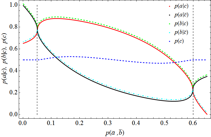
Figure 1: For three random variables $A=\{a,\bar{a}\}$, $B=\{b,\bar{b}\}$ and $C=\{c,\bar{c}\}$, this figure presents conditional probabilities in (11, 12) for a concrete numerical example $p(a,\bar{b})=p(\bar{a},b)=0.175$, where $0\leq p(\bar{a},\bar{b})\leq 0.65$. Thus $A$ and $B$ are correlated for $0.0511<p(\bar{a},\bar{b})<0.5989$ and are anti-correlated for $0<p(\bar{a},\bar{b})<0.0511$ and $0.5989<p(\bar{a},\bar{b})<0.65$; cf. (11, 12). Curves that are depicted close are in reality coinciding. The curve for $p(c)$ is seen to be non-monotonic with one global maximum and one global minimum.
The maximization of $L_{\beta\lesssim 1}$ in (4, 5) was carried out under additional condition $p(b|c)>p(b|\bar{c})$ that secures a continuous transition between correlated and anti-correlated situations. Several quantities are non-analytic along this transition, e.g. $p(b|c)$, $p(b|\bar{c})$, and $p(c)$. In particular, $p(c)=1/2$ in the anti-correlated situation.

IV Most likely common cause for three variables

IV.1 Definition of the problem

Let us now assume that $A$ in (1) consists of two random variables $A=(A_{1},A_{2})$, where $A_{1}=\{a_{1}\}$ and $A_{2}=\{a_{2}\}$. Now we are given an observed probability $p(a_{1},a_{2},b)$ and look for the most likely common cause $C$ for $A$ and $B$:

$$p(a_{1},a_{2},b,c)=p(a_{1},a_{2},c)p(b|c),\quad t_{C}<{\rm min}[t_{A_{1}},t_{A_{2}},t_{B}],$$ (19)

where random variables refer to times $t_{A_{1}}$, $t_{A_{2}}$, $t_{B}$, and $t_{C}$, respectively. Relations between $t_{A_{1}}$, $t_{A_{2}}$, and $t_{B}$ depend on concrete examples.

Note that joining two variables $A_{1}$ and $A_{2}$ into one $A$ is not a trivial operation. It does imply that $A_{1}$ and $A_{2}$ are closer to each other than each of them to $B$; e.g. $A_{1}$ and $A_{2}$ are contiguous in space or time or do belong to the same system. Here are two examples: (i) $A_{1}$ – grades of examination, $A_{2}$ – preliminary estimate of this grade, $B$ – name of a student arrived to examination, $C$ – knowledge gained before the examination; here $t_{A_{1}}>t_{B}>t_{A_{2}}>t_{C}$. (ii) $A_{1}$ – cerebrovascular issues, $A_{2}$ – cardiovascular issues, $B$ – susceptibility to stresses, $C$– genetic predisposition; now $t_{A_{1}}>t_{B}>t_{C}$ and $t_{A_{2}}>t_{B}>t_{C}$.

IV.2 Two extreme cases of initial 3-variable correlations

We focus on two extreme cases of three-variable correlations in $p(a_{1},a_{2},b)$. The first case when $A_{2}$ screens $A_{1}$ from $B$:

$$p(a_{1},b|a_{2})=p(a_{1}|a_{2})p(b|a_{2}).$$ (20)

The second case when $A_{1}$ and $A_{2}$ are marginally independent:

$$p(a_{1},a_{2},b)=p(b|a_{1},a_{2})p(a_{1})p(a_{2}).$$ (21)

These two cases are representative in the following sense. Generic three-variable correlations in $p(a_{1},a_{2},b)$ can be quantified via triple information $I(A_{1}:A_{2}:B)$ that (in contrast to the two-variable mutual information that is always non-negative) can assume both negative and positive values; see Appendix D for details. Moreover, three-variable correlations can be classified via the sign of $I(A_{1}:A_{2}:B)$. Now (21) is a representative example of $I(A_{1}:A_{2}:B)<0$, while (20) is an example of $I(A_{1}:A_{2}:B)>0$; cf. Appendix D.

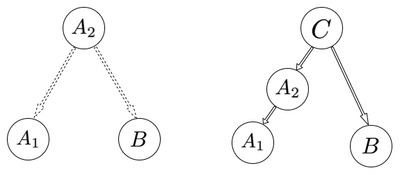
Figure 2: The left Causal Markov Conditioned Directed Acyclic Graph (DAG) denotes the correlation structure in (20). The right DAG denotes the correlation structure implied by the most likely cause $C$ of $A=(A_{1},A_{2})$ and $B$; see (23).

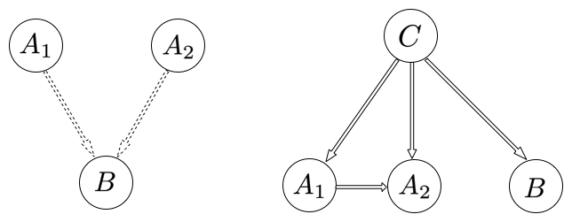
Figure 3: The left Causal Markov Conditioned Directed Acyclic Graph (DAG) denotes the correlation structure in (21). The right DAG denotes the correlation structure implied by the most likely cause $C$ of $A=(A_{1},A_{2})$ and $B$.

Applying the maximization of $L_{\beta\lesssim 1}$ to (20) we get that the maximum is achieved for [see Appendix E for derivation]:

$$p(c|a_{1},a_{2})=p(c|a_{2}).$$ (22)

Supplementing (22) with the common cause definition (19) we find for the most likely cause:

$$p(a_{1},a_{2},b,c)=p(a_{1},a_{2},c)p(b|c)=p(c)p(a_{2}|c)p(a_{1}|a_{2})p(b|c),$$ (23)

which means that (23) can be depicted by the right graph in Fig. 2; see (22). Quantities in the right-hand-side of (23) are found from the maximization of $L_{\beta\lesssim 1}$, and do not have other general regularities. Note that (22) implies for mutual informations

$$I(A_{1}:A_{2}|C)\equiv\sum_{a_{1},a_{2},c}p(a_{1},a_{2},c)\ln\frac{p(a_{1},a_{2}|c)}{p(a_{1}|c)p(a_{2}|c)}=I(A_{1}:A_{2})-I(A_{1}:C)<I(A_{1}:A_{2}),$$ (24)

which means that not only global correlations are explained by the most likely cause (i.e. $I(A_{1}A_{2}:B|C)=0$), but also local correlations (i.e. the correlations between $A_{1}$ and $A_{2}$) are partially explained by the most likely cause $C$.

When looking for the most likely common cause of (21) one would expect to get $p(a_{1},a_{2}|c)=p(a_{1}|c)p(a_{2}|c)$ in addition to the common cause definition (19). This is however not the case : the maximization of $L_{\beta\lesssim 1}$ produces (19), where $p(a_{1},a_{2},c)$ does not have any specific structure. In particular, we have now

$$0=I(A_{1}:A_{2})\leq I(A_{1}:A_{2}|C).$$ (25)

We checked that a generic $p(a_{1},a_{2},c)$ is also obtained for two other non-trivial cases related to respectively (20) and (21):

$$p(a_{1},a_{2},b)=p(b)p(a_{1}|b)p(a_{2}|b),$$ (26)

$$p(a_{1},a_{2},b)=p(b)p(a_{2})p(a_{1}|a_{2},b).$$ (27)

IV.3 DAGs and TODAGs

Let us now show how the obtained results can be interpreted in terms of Markov Conditioned Directed Acyclic Graphs scheines ; berko . We shall call them simply DAGs and emphasize that any DAG can be employed in two different senses; see e.g. scheines ; verma . First, it can only reflect the correlation structure present; e.g. there are three DAGs that refer to (20). One of them is the open fork shown in the left Fig. 2, while another two of them are $A_{1}\to A_{2}\to B$ and $B\to A_{2}\to A_{1}$. The choice of DAG is reduced after it is postulated that the arrows of DAG coincide with the flow of time. For example, the unique DAG that refers to (20) with condition $t_{A_{1}}<t_{A_{2}}<t_{B}$ is $A_{1}\to A_{2}\to B$. We shall call it time-ordered DAG (TODAG), whenever the emphasis is needed. But now it is possible that no TODAG exists for the given correlation structure; e.g. (21) cannot be represented via a TODAG, if $t_{B}<t_{A_{1}}$ or $t_{B}<t_{A_{2}}$; cf. the left Fig. 3. This is excluded from consideration as a non-generic situation scheines . For this specific example, the exclusion is perhaps understandable, since it is empirically not expected to find two independent later variables influenced by an earlier one.

Returning to (23), we see (given our basic assumption $t_{C}<{\rm min}[t_{A_{1}},t_{A_{2}},t_{B}]$) that it can be described via a TODAG only for $t_{A_{2}}<t_{A_{1}}$. Whenever $t_{A_{2}}>t_{A_{1}}$ no TODAG exists that corresponds to (23). Note that the observed probability (20) for $t_{B}>t_{A_{2}}>t_{A_{1}}$ refers to a well-defined TODAG: $A_{1}\to A_{2}\to B$.

In contrast, $p(a_{1},a_{2},b,c)$ produced as the most likely cause from (21) does always have a unique TODAG, because $p(a_{1},a_{2},c)$ is generic, and we assume that $t_{C}$ is the earliest time. This TODAG is unique even if for (21) no TODAG exists due to e.g. $t_{B}<t_{A_{1}}$. Thus, DAGs that refer to (20, 21) produce quite different most likely common causes.

V Predictive likelihood, minimum entropy, and sparse common cause

V.1 Predictive (maximum aposteriori) likelihood

In section II we defined the generalized likelihood $L_{\beta}$ and argued that it is a concave function of $\beta$ for $\beta<1$; see (3). Choosing $\beta\lesssim 1$ was motivated by this concavity, closeness to the marginal likelihood $L_{\beta=1}$, and relations with the maximum entropy method. We can also consider maximization of $L_{\beta>1}$ motivating it as follows from (3). Once in the joint probability $p_{\theta}(a,b,c)$ the hidden variable $c$ is unknown, we can estimate it via the maximum aposteriori method: given the observed $(a,b)$ we find

$${\rm argmax}_{c}[p_{\theta}(a,b,c)]=\hat{c}(a,b,\theta).$$ (28)

Eq. (28) implies that some $c$ is kept fixed when generating each $(a,b)$, which may or may not hold true. Putting (28) back into $p_{\theta}(a,b,c)$ we find unknown $\theta$ via the predictive likelihood predo :

$$\hat{\theta}={\rm argmax}\Big{[}\sum_{a,b}p(a,b)\ln p_{\theta}(a,b,\hat{c}(a,b,\theta))\Big{]}={\rm argmax}\Big{[}L_{\beta\to\infty}\Big{]},$$ (29)

where we expressed $\hat{\theta}$ via $L_{\beta\to\infty}$ by noting from (3): $\sum_{c}p^{\beta}_{\theta}(a,b,c)=p^{\beta}_{\theta}(a,b,\hat{c}(a,b,\theta))$, which is valid in the limit $\beta\to\infty$. Note from (4, 9) that ${\rm max}[L_{\beta\gtrsim 1}]$ is equivalent to minimizing the full entropy $H(ABC)$.

Recall that $\theta$ amounts to unknown probabilities $p(a,c)$ and $p(b|c)$, as discussed in (4). Now the maximization of $L_{\beta>1}$ is straightforward. We shall illustrate it for binary variables $A=\{a,\bar{a}\}$, $B=\{b,\bar{b}\}$, and $C=\{c,\bar{c}\}$. Take the first term in $L_{\beta>1}$ and note that

$$p(a,b)\ln\Big{(}\Big{[}p^{\beta}(a,c)p^{\beta}(b|c)+p^{\beta}(a,\bar{c})p^{\beta}(b|\bar{c})\Big{]}^{\beta}\Big{)}\leq p(a,b)\ln\Big{(}p(a,c)p(b|c)+p(a,\bar{c})p(b|\bar{c})\Big{)}=p(a,b)\ln p(a,b).$$ (30)

where we employed constraints (5). Similar inequalities hold for every term in $L_{\beta>1}$. Hence, the maximization of $L_{\beta>1}$ is achieved for one of the following two solutions, where $\leq$ in (30) is satisfied as $=$:

$$p(a,c)=p(\bar{a},\bar{c})=0,$$ (31)

$$p(b,c)=p(\bar{b},\bar{c})=0.$$ (32)

They are equivalent since they provide the same maximal value ${\rm max}[L_{\beta>1}]=\sum_{k=a,\bar{a};l=b,\bar{b}}p(k,l)$. Another two solutions are found from (31, 32) by interchanging there $c$ with $\bar{c}$; this symmetry is anyhow always present. Note that neither (31, 32) nor ${\rm max}[L_{\beta>1}]$ depend on $\beta$ provided that $\beta>1$.

V.2 Minimum entropy

For inferring the unknown common cause $C$, Ref. murad proposed to minimize the entropy $H(C)=-\sum_{c}p(c)\ln p(c)$ of $C$. The rationale of this is that $C$ is made to be possibly deterministic: the absolute minimum $H(C)=0$ is reached for a deterministic $C$, where only one probability among $\{p(c)\}$ is non-zero.

We found analytically (see Appendix F) that for binary $A$, $B$ and $C=\{c,\bar{c}\}$, the minimization of $H(C)=-p(c)\ln p(c)-p(\bar{c})\ln p(\bar{c})$ under conditions (5) produces

$$p(a|c)=p(b|c)=0,$$ (33)

$$p(\bar{a}|c)=p(\bar{b}|c)=0,$$ (34)

for the correlated situation:

$$p(a,b)-p(a)p(b)=p(\bar{a},\bar{b})-p(\bar{a})p(\bar{b})=p(a,b)p(\bar{a},\bar{b})-p(a,\bar{b})p(\bar{a},b)>0.$$ (35)

For the anticorrelated situation when the sign in (35) is inverted, we get

$$p(\bar{a}|c)=p(b|c)=0,$$ (36)

$$p(a|c)=p(\bar{b}|c)=0.$$ (37)

The meaning of (33–37) is as follows. We find $p(c)$ from (5, 33) and place this into $H(C)$. The same is repeated with (5, 34), and the two $H(C)$ are compared to each other. We take the solution with the smallest $H(C)$ as the actual ${\rm argmin}\Big{[}H(C)\Big{]}$; see Appendix F. The same is done with (5, 36) and (5, 37)

V.3 Defects of sparse common cause

Note that (31, 32) and (33–37) are similar to each other in the following sense of sparsity: both assume the maximal number of zeros in $p(a,c)$ and $p(b|c)$ so that conditions (5) provide a unique solution for given $\{p(a,b),p(a,\bar{b}),p(\bar{a},b),p(\bar{a},\bar{b})\}$.

Whether (31, 32) or (33–37) should be preferred to the solution found via ${\rm max}[L_{\lesssim 1}]$? In our opinion no, since (31, 32) and (33–37) imply a mixture of deterministic and fine-tuned event causation [cf. section III.2] with probabilistic causation. Such a mixture is not realistic; i.e. it needs prior information.

In addition, the common cause holding one of (33–37) has the following defect which is absent in (31). Recall an important implication of the common cause principle that demands $p(b,c)>0$ for all $(b,c)$; cf. the discussion after (1). This condition is clearly violated both for each solution in (33–37); i.e. the common cause loses an important aspect of its meaning. In contrast, condition $p(b,c)>0$ holds for (31).

Hence, even if a sparse common cause is searched for, we recommend the solution found via the predictive maximum likelihood, and not the one obtained via minimum entropy of $C$.

VI Summary

Using the generalized likelihood (GL) method, we determine the most probable unbiased cause $C=\{c\}$ for a given joint probability $p(a,b)$ of observed variables (effects) $A=\{a\}$ and $B=\{b\}$. This can serve as a reference point for causal inference, and also explains which causes are likely to see in practice. The choice to employ GL relates to the maximum entropy principle and is motivated by the non-identifiability of the problem. The results obtained from both numerical and analytical analyses affirm the effectiveness of the suggested approach. Notably, we observe an interesting phase transition-like behavior in the minimal setup when transitioning from anticorrelated to correlated $p(a,b)$. Furthermore, we present cases where the identified parameters can be interpreted in terms of time-ordered Directed Acyclic Graphs (TODAGs), as well as cases where such interpretation is not possible. We also compared our results with the minimum common cause entropy approach and identified disadvantages of that approach compared to predictions of GL and of the predictive likelihood.

As a direction for future research, we suggest investigating the dependence of the GL function on the dimensionality of the common cause. We intend to explore potential applications in our future studies.

Appendix A Common cause principle and its evolution

Reichenbach reich formulated the common cause principle with respect to three distinct events $a$, $b$ and $c$; their joint probability is $p(a,b,c)$. The definition amounts to the following 4 conditions reich ; suppes ; billi ; berko ; szabo ; mazz ; sterg .

1. The causal influence from $a$ to $b$ and from $b$ to $a$ are excluded. To this end, it is sufficient that the events a and b take place at equal times, or that they are space-like, i.e. no interaction could effectively relate $a$ and $b$. Naturally, $c$ refers to an earlier time, i.e. $c$ is in the common past of $a$ and $b$.

2. The correlation between $a$ and $b$ holds reich :

   $$p(ab)>p(a)p(b).$$ (38)

3. $c$ and $\bar{c}$ screen-off correlations between $a$ and $b$:

   $$p(ab|c) =p(a|c)p(b|c),$$ (39)

   $$p(ab|\bar{c}) =p(a|\bar{c})p(b|\bar{c}),$$ (40)

   where $\bar{c}$ is the complement of $c$, i.e. the event $\bar{c}$ takes place when $c$ does not and vice versa.

4. $c$ increases the probability of $a$ $(b)$ compared to $\bar{c}$

   $$p(a|c)>p(a|\bar{c}),$$ (41)

   $$p(b|c)>p(b|\bar{c}).$$ (42)

The following objections were made against these conditions berko ; uffink .

– It is not clear why specifically the correlation condition (38) is taken for defining correlations that need explanations; anti-correlations also need explanations.

– If we accept (38), conditions (41, 42) are redundant, because one can write using (39, 40):

$$p(ab)-p(a)p(b)=p(c)p(\bar{c})[p(a|c)-p(a|\bar{c})][p(b|c)-p(b|\bar{c})],$$ (43)

i.e. if (38) is accepted, then either $c$ or $\bar{c}$ is a common cause, there is no need to impose (41, 42) separately.

– The existence of a single common cause ($c$ or $\bar{c}$) is too restrictive, so people moved to common cause systems, where instead of two events with probabilities $p(c)+p(\bar{c})=1$, one employs a larger set of events $\{c\}$ with $\sum_{c}p(c)=1$ szabo . Conditions (39, 40) generalize easily:

$$p(a,b|c)=p(a|c)p(b|c)\quad\text{for all}\quad c.$$ (44)

Note that conditions (41, 42) do not extend uniquely to this more general situation: there are at least two candidates for such an extension and the choice between them is not unique sterg ; mazz .

– Reichenbach’s formulation combines two different things: correlations that need to be explained via events $c$ and $\bar{c}$, and event causation expressed by (41, 42). The understanding of the event causation is blurred by Simpson’s and related paradoxes berko ; billi . Some of them question whether the cause need to increase the probability of its effect hesslow ; beebee . Hence, it is useful to separate explicitly the explanation of correlations from the event causation. It is also natural to avoid the restriction of doing only two specific values $a$ and $b$ for two random variables $A$ and $B$: we can require (44) for all values of $A$ and $B$ under fixed $c$ uffink . Once this is done, then we have to skip the condition (38) as well, because it cannot hold for all values of the random variables $A$ and $B$. Summing up, we converge to the definition given in section I.

Appendix B Maximum likelihood and nonidentifiablity

Recall the usual setup of parameter estimation cox_hinkley . We want to estimate the unknown parameters $\theta$ in the probability $p_{\theta}(x)={\rm Pr}(X=x)$ of the random variable $X=\{x\}$. The estimation is done from a i.i.d. sample $(x_{1},x_{2},\dots,x_{N})$. These parameters can be estimated by maximizing over $\theta$ the likelihood function cox_hinkley :

$$\mathcal{L}_{N}(\theta)=\frac{1}{N}\sum_{i=1}^{N}\ln p_{\theta}(x_{i}).$$ (45)

According to the law of large numbers, for $N\gg 1$ the frequencies of various values in the sample coincide with the true probabilities, so we can rewrite (45) as

$$\mathcal{L}_{N}(\theta)=\sum_{x}p_{\theta^{*}}(x)\ln p_{\theta}(x),$$ (46)

where $\theta^{*}$ are the true parameters with which the sample was generated. The following relation obviously holds

$$\underset{\theta}{\arg\max}\sum_{x}p_{\theta^{*}}(x)\ln p_{\theta}(x)=\underset{\theta}{\arg\min}\sum_{x}p_{\theta^{*}}(x)\ln\frac{p_{\theta^{*}}(x)}{p_{\theta}(x)}.$$ (47)

Since the relative entropy $\sum_{x}p_{\theta^{*}}(x)\ln\frac{p_{\theta^{*}}(x)}{p_{\theta}(x)}\geq 0$ nullifies only for

$$p_{\theta}(x)=p_{\theta^{*}}(x),~{}~{}{\rm for~{}~{}all}~{}~{}x,$$ (48)

the maximizer of (46) holds (48). Now if (48) implies

$$\theta=\theta^{*},$$ (49)

the model is called identifiable cox_hinkley . Otheriwse, when (48) holds, but (49) does not, the model is called non-identifiable.

Appendix C No causes for independent events

Consider the uncoupled situation:

$$p(a,b)=p(a)p(b),$$ (50)

and assume that we look for the common cause by maximizig the generalized likelihood:

$$L_{\beta}=\frac{1}{\beta}\sum_{ab}p(a,b)\ln\sum_{c}p^{\beta}(c)p^{\beta}(a|c)p^{\beta}(b|c),$$ (51)

$$\sum_{c}p(c)p(a|c)p(b|c)=p(a,b).$$ (52)

Using (50, 52) we find for (51):

$$L_{\beta}=\sum_{a}p(a)\ln p(a)+\sum_{b}p(b)\ln p(b)$$

$$+\frac{1}{\beta}\sum_{ab}p(a)p(b)\ln\sum_{c}\pi^{\beta}(c|a,b),$$ (53)

$$\pi(c|a,b)=\frac{p(c|a)p(c|b)}{p(c)},$$ (54)

where the constraint

$$\sum_{c}\pi(c|a,b)=1$$ (55)

on $\pi(c|a,b)$ follows from (52). Note that constraint (54) does not depend on $(a,b)$. We now have:

$${\rm max}[L_{\beta}]=\sum_{a}p(a)\ln p(a)+\sum_{b}p(b)\ln p(b)$$

$$+\frac{1}{\beta}{\rm max}\left(\sum_{ab}p(a)p(b)\ln\sum_{c}\pi^{\beta}(c|a,b)\right)$$ (56)

$$\leq\sum_{a}p(a)\ln p(a)+\sum_{b}p(b)\ln p(b)$$ (57)

$$+\frac{1}{\beta}\sum_{ab}p(a)p(b)\,{\rm max}\left(\ln\sum_{c}\pi^{\beta}(c|a,b)\right).$$ (58)

In view of (55), the maximization in (58) is straightforward: $\ln\sum_{c}\pi^{\beta}(c|a,b)$ is a concave function of $\pi(c|a,b)$ for $\beta<1$, because it is made of concave functions. Hence the unique maximum of $\ln\sum_{c}\pi^{\beta}(c|a,b)$ is

$$\pi(c|a,b)=\frac{1}{n},\qquad\sum_{c=1}^{n}\frac{1}{n}=1,$$ (59)

which obviously saturates the inequality in (57).

Eqs. (58, 59) imply:

$$p(c|a)=p(c|b)=p(c)=\frac{1}{n},$$ (60)

$${\rm max}[L_{\beta}]=\sum_{a}p(a)\ln p(a)+\sum_{b}p(b)\ln p(b)+\frac{1-\beta}{\beta}\ln n,$$ (61)

where (60) means that the method predicts no cause, as it should.

The same method that led us to (61) can be employed for establishing generally not reachable upper bound on ${\rm max}[L_{\beta}]$. Indeed, note that (51, 52) can be written as

$$L_{\beta}=\sum_{ab}p(a,b)\ln p(a,b)+\frac{1}{\beta}\sum_{ab}p(a,b)\ln\sum_{c}\pi^{\beta}(c|a,b),$$ (62)

$$\pi(c|a,b)=p(c)p(a|c)p(b|c)/p(a,b),\qquad\sum_{c}\pi(c|a,b)=1.$$ (63)

Then (62) implies with the same method as for (61):

$${\rm max}[L_{\beta}]\leq\sum_{ab}p(a,b)\ln p(a,b)+\frac{1}{\beta}\sum_{ab}p(a,b)\,{\rm max}\left(\ln\sum_{c}\pi^{\beta}(c|a,b)\right),$$ (64)

$$=\sum_{a,b}p(a,b)\ln p(a,b)+\frac{1-\beta}{\beta}\ln n,$$ (65)

where the maxima in the last equation of (64) are reached for $\pi(c|a,b)=1/n$, which leads to $p(c)=\frac{1}{n}$. However, these two equations are consistent with the screening condition for $C$ only for $p(a,b)=p(a)p(b)$. This means that for $p(a,b)\not=p(a)p(b)$, (65) is an upper bound for ${\rm max}[L_{\beta}]$.

Let us now generalize the above conclusion. Assume the following situation:

$$L_{\beta}=\frac{1}{\beta}\sum_{a_{1}a_{2}b}p(a_{1})p(a_{2},b)\ln\sum_{c}p^{\beta}(a_{1},a_{2},c)p^{\beta}(b|c),$$ (67)

$$\sum_{c}p(a_{1},a_{2},c)p(b|c)=p(a_{1})p(a_{2},b).$$

Now (67) can be written as

$$L_{\beta}=\sum_{a_{1}}p(a_{1})\ln p(a_{1})+\frac{1}{\beta}\sum_{a_{1}}p(a_{1})\sum_{a_{2}b}p(a_{2},b)\ln\sum_{c}p^{\beta}(a_{2},c|a_{1})p^{\beta}(b|c),$$ (68)

$$\sum_{c}p(a_{2},c|a_{1})p(b|c)=p(a_{2},b).$$ (69)

Hence we find:

$${\rm max}[L_{\beta}]=\sum_{a_{1}}p(a_{1})\ln p(a_{1})+\frac{1}{\beta}{\rm max}\left(\sum_{a_{1}}p(a_{1})\sum_{a_{2}b}p(a_{2},b)\ln\sum_{c}p^{\beta}(a_{2},c|a_{1})p^{\beta}(b|c)\right)$$

(70)

$$\leq\sum_{a_{1}}p(a_{1})\ln p(a_{1})+\frac{1}{\beta}\sum_{a_{1}}p(a_{1}){\rm max}\left(\sum_{a_{2}b}p(a_{2},b)\ln\sum_{c}p^{\beta}(a_{2},c|a_{1})p^{\beta}(b|c)\right).$$ (71)

It is clear from (67) that the maximum in (71) is reached for

$$p(a_{2},c|a_{1})=p(a_{2},c).$$ (72)

This also means that the inequality in (71) is satisfied. Hence the maximization in (70) is solved via (72), where $p(a_{2},c)$ is found from the restricted maximization:

$$\frac{1}{\beta}{\rm max}\left(\sum_{a_{2}b}p(a_{2},b)\ln\sum_{c}p^{\beta}(a_{2},c)p^{\beta}(b|c)\right),$$ (73)

$$\sum_{c}p(a_{2},c)p(b|c)=p(a_{2},b).$$ (74)

Appendix D Triple information: remainder

The triple information $I(A_{1}:A_{2}:B)$ quantifies three-variable correlations present in $p(a_{1},a_{2},b)$ triple ; triple_f :

$$I(A_{1}:A_{2}:B) = I(A_{1}:A_{2})-I(A_{1}:A_{2}|B)$$ (75)

$$= I(A_{1}:B)+I(A_{2}:B)-I(A_{1}A_{2}:B)$$ (76)

$$= H(A_{1})+H(A_{2})+H(B)-H(A_{1}A_{2})-H(A_{2}B)-H(A_{1}B)+H(A_{1}A_{2}B),$$ (77)

where $H(A_{1}A_{2}B)$ is the joint entropy of random variables $A_{1}$, $A_{2}$ and $B$, and $I(A_{1}:B)$ is the mutual information. $I(A_{1}:A_{2}:B)$ is the change of the mutual information between any pair, e.g. $A_{1}$ and $A_{2}$, when introducing the context of $B$; see (75). Eq. (77) shows that $I(A_{1}:A_{2}:B)$ has a set-theoretic meaning of triple overlap, and is invariant with respect to any permutation of the sequence $A_{1},A_{2},B$. Eq. (76) shows that $I(A_{1}:A_{2}:B)$ also quantifies the sub-additivity of the mutual information with respect to joining any pair of the three random variables.

$I(A_{1}:A_{2}:B)$ becomes zero when at least one random variable is independent from others, e.g., $p(a_{1},a_{2},b)=p(a_{1},a_{2})p(b)$. In contrast to two-variable correlations quantified by $I(A_{1}:A_{2})\geq 0$ [$I(A_{1}:A_{2})=0$ only when $A_{1}$ and $A_{2}$ are independent], $I(A_{1}:A_{2}:B)$ can have either sign. Now $I(A_{1}:A_{2}:B)>0$ means the informations contained in the correlations $A_{1}:B$ and $A_{2}:B$ are [mutually] redundant, since when joining $A_{1}$ and $A_{2}$, the resulting mutual information decreases; cf. (76). Analogously, $I(A_{1}:A_{2}:B)<0$ means that by joining $A_{1}$ and $A_{2}$ one creates information that was absent in $A_{1}:B$ and $A_{2}:B$ separately: the whole is more than the sum of its parts triple ; triple_f ; neural . This scenario relates to the physical concept of frustration triple_f , and finds applications in neuroscience neural .

Appendix E Derivation of Eq. (22)

Consider the case when the joint probability of $A_{1}$, $A_{2}$ and $B$ holds (20). This situation can be modeled with $p(a,b)=p(a_{2})p(a_{1}|a_{2})p(b|a_{2})$. Below we will prove that the most likely common cause (19) for this situation satisfies (22). Starting from (4, 5) we note that in

$$L_{\beta}=\frac{1}{\beta}\sum_{a_{1},a_{2},b}p(a_{1},a_{2})p(b|a_{2})\ln{\sum_{c}p^{\beta}(a_{1},a_{2},c)p^{\beta}(b|c)}=\sum_{a_{1},a_{2}}p(a_{1},a_{2})\ln{p(a_{1},a_{2})}$$ (78)

$$+\frac{1}{\beta}\sum_{a_{1},a_{2},b}p(a_{2})p(a_{1}|a_{2})p(b|a_{2})\ln{\sum_{c}p^{\beta}(c|a_{1},a_{2})p^{\beta}(b|c)},$$ (79)

only (79) need to be optimized. Using the concavity of $L_{\beta<1}$ we have in (78):

$$\begin{split}&\sum_{a_{2}}p(a_{2})\sum_{a_{1}}p(a_{1}|a_{2})\ln{\sum_{c}p^{\beta}(c|a_{1},a_{2})p^{\beta}(b|c)}\leq\sum_{a_{2}}p(a_{2})\ln{\sum_{c}(\sum_{a_{1}}p(a_{1}|a_{2})p(c|a_{1},a_{2}))^{\beta}p^{\beta}(b|c)}\\ &=\sum_{a_{2}}p(a_{2})\ln{\sum_{c}p^{\beta}(c|a_{2})p^{\beta}(b|c)}.\end{split}$$ (80)

Now constraints (5) together with (20) can be written as

$$p(b|a_{2})=\sum_{c}p(c|a_{1},a_{2})p(b|c),\quad\sum_{b}p(b|c)=1.$$ (81)

Assume that the maximization of (79) under constraints (81) resulted in $\hat{p}(c|a_{1},a_{2}),\hat{p}(b|c)$. Obviously, the inequality (LABEL:concineq) holds also for the maximizers

$$\sum_{a_{2}}p(a_{2})\sum_{a_{1}}p(a_{1}|a_{2})\ln{\sum_{c}\hat{p}^{\beta}(c|a_{1},a_{2})\hat{p}^{\beta}(b|c)}\leq\sum_{a_{2}}p(a_{2})\ln{\sum_{c}\hat{p}^{\beta}(c|a_{2})\hat{p}^{\beta}(b|c)}.$$ (82)

On the other hand, we can maximize (79) with an additional constraint

$$p(c|a_{1},a_{2})=\hat{p}(c|a_{2}).$$ (83)

Since (83) is compatible with (81), it can only decrease the value of maximum:

$$\max_{p(c|a_{1},a_{2})p(b|c)}\left[{\frac{1}{\beta}\sum_{a_{1},a_{2},b}p(a_{2})p(a_{1}|a_{2})\ln{\sum_{c}p^{\beta}(c|a_{1},a_{2})p^{\beta}(b|c)}}\right]\geq\frac{1}{\beta}\sum_{a_{2},b}p(a_{2})\ln{\sum_{c}\hat{p}^{\beta}(c|a_{2})\hat{p}^{\beta}(b|c)}.$$ (84)

Comparing (84) with (82) we get

$$\max_{p(c|a_{1},a_{2})p(b|c)}\left[{\frac{1}{\beta}\sum_{a_{1},a_{2},b}p(a_{2})p(a_{1}|a_{2})\ln{\sum_{c}p^{\beta}(c|a_{1},a_{2})p^{\beta}(b|c)}}\right]=\frac{1}{\beta}\sum_{a_{2},b}p(a_{2})\ln{\sum_{c}\hat{p}^{\beta}(c|a_{2})\hat{p}^{\beta}(b|c)}.$$ (85)

Thus, we deduced that the maximum is achieved for [cf. (22)]

$$\hat{p}(c|a_{1},a_{2})=\hat{p}(c|a_{2}).$$ (86)

Appendix F Minimization of the entropy $H(C)$ of $C$ for 3 binary variables $A$, $B$, and $C$

Consider the common cause set-up (1) for binary variables $A=\{a,\bar{a}\}$, $B=\{b,\bar{b}\}$, and $C=\{c,\bar{c}\}$. Start from

$$p(a,b)=p(c)p(a|c)p(b|c)+[1-p(c)]p(a|\bar{c})p(b|\bar{c}),$$ (87)

$$p(a)=p(c)p(a|c)+[1-p(c)]p(a|\bar{c}),$$ (88)

$$p(b)=p(c)p(b|c)+[1-p(c)]p(b|\bar{c}).$$ (89)

Find $p(a|\bar{c})$ from (88) and $p(b|\bar{c})$ from (89) and put them into (87) so as to express $p(c)$ via unknown $p(a|c)$ and $p(b|c)$:

$$p(c) = \frac{p(a,b)-p(a)p(b)}{p(a|c)p(b|c)-p(b)p(a|c)-p(a)p(b|c)+p(a,b)}$$ (91)

$$\leq{\rm min}\Big{[}\frac{p(a)}{p(a|c)},\frac{1-p(a)}{1-p(a|c)},\frac{p(b)}{p(b|c)},\frac{1-p(b)}{1-p(b|c)}\Big{]},$$

where the inequalities in (91) comes from $0\leq p(a|\bar{c})\leq 1$ and $0\leq p(b|\bar{c})\leq 1$.

To minimize $H(C)=-p(c)\ln p(c)-[1-p(c)]\ln[1-p(c)]$ means to maximize ${\rm max}[p(c),1-p(c)]$, i.e. to maximize $p(c)$, if $p(c)>1/2$, and to minimize it if $p(c)<1/2$. Hence, we shall find optimas (minimas or maximas) of $p(c)$, and then select the one with the smallest $H(C)$. As seen from (91), optimas of $p(c)$ as a function of $p(a|c)$ and $p(b|c)$ coincide with those of

$$p(a|c)p(b|c)-p(b)p(a|c)-p(a)p(b|c)+p(a,b).$$ (92)

The Hessian of (92) over $p(a|c)$ and $p(b|c)$ under $0<p(a|c)<1$ and $0<p(b|c)<1$ refers to a saddle point. Hence optimas of (92) are reached at the boundaries and amount to one of the following 4 solutions:

$$p(a|c)=p(b|c)=0,$$ (93)

$$p(a|c)=p(b|c)=1,$$ (94)

$$p(a|c)=1,\quad p(b|c)=0,$$ (95)

$$p(a|c)=0,\quad p(b|c)=1.$$ (96)

It is seen from (91) that (93, 94) produce (respectively)

$$p(c)=\frac{p(a,b)-p(a)p(b)}{p(a,b)},$$ (97)

$$p(c)=\frac{p(\bar{a},\bar{b})-p(\bar{a})p(\bar{b})}{p(\bar{a},\bar{b})}.$$ (98)

Hence (93, 94) refer to the correlated situation:

$$p(a,b)-p(a)p(b)=p(\bar{a},\bar{b})-p(\bar{a})p(\bar{b})=p(a,b)p(\bar{a},\bar{b})-p(a,\bar{b})p(\bar{a},b)>0.$$ (99)

To find the actual solution under condition (99), we should select in (97, 98), $p(c)$ that provides the smallest $H(C)=-p(c)\ln p(c)-[1-p(c)]\ln[1-p(c)]$.

Likewise, (95, 96) refer to the anti-correlated situation, when the sign in (99) is inverted. It should be clear that (97, 98) do not apply to the anti-correlated situation, because they predict $p(c)<0$.

We emphasize that in all cases (93–96), constraint (91) holds automatically.

References

• (1) G. Hesslow, Two Notes on the Probabilistic Approach to Causality, Philosophy of Science, 43, 290-292 (1976).
• (2) H. Reichenbach, The Direction of Time (Dover Publications Inc., New York, 1956 [1999]).
• (3) P. Suppes, A probabilistic theory of causality (North-Holland, Amsterdam, 1970).
• (4) J. Williamson, Probabilistic Theories of Causality, In The Oxford Handbook of Causation, ed. by H. Beebee, C. Hitchcock, and P. Menzies (Oxford University Press, NY, 2009).
• (5) J. Berkovitz, On Causal Inference in Determinism and Indeterminism, in H. Atmanspacher and R. Bishop (eds.), Between Chance and Choice: Interdisciplinary Perspectives on Determinism, Imprint Academic, pp. 237-278 (2002).
• (6) G. Hofer-Szabo, M. Redei, and L.E. Szabo, The Principle of the Common Cause (Cambridge University Press, Cambridge, 2013).
• (7) C. Mazzola, Reichenbachian common cause systems revisited Found. Phys. 42, 512–523, (2012)
• (8) C. Stergiou, Explaning Correlations by Partitions, Found. Phys. 45, 1599-1612 (2015).
• (9) O. Penrose, The Direction of Time, in Chance in Physics: Foundations and Perspectives, edited by J. Bricmont, D. Durr, M. C. Galavotti, G. C. Ghirardi, F. Petruccione and N. Zanghi (Springer-Verlag, Berlin 2001).
• (10) K.B. Wharton and N. Argaman, Colloquium: Bell’s theorem and locally mediated reformulations of quantum mechanics, Reviews of Modern Physics, 92, 021002 (2020).
• (11) R. Balian, From microphysics to macrophysics, I, II, (Springer, Berlin, 2007).
• (12) E. Sober, Venetian Sea Levels, British Bread Prices, and the Principle of the Common Cause, Brit. J. Phil. Sci. 52 331-346 (2001).
• (13) K.D. Hoover, Nonstationary Time Series, Cointegration, and the Principle of the Common Cause, The Brit. J. Phil. Science, 54, 527–551 (2003).
• (14) P. Spirtes, C.N. Glymour, and R. Scheines, Causation, Prediction, and Search (MIT Press, 2000).
• (15) A. Allahverdyan, Observational nonidentifiability, generalized likelihood and free energy, 125, 118-138, (2020).
• (16) J. Bjornstad, Predictive likelihood: A Review (with discussion), Statistical Science, 5, 242-265 (1990).
• (17) G.U. Yule, Notes on the theory of association of attributes in statistics, Biometrika, 2, 121-134 (1903).
• (18) D. R. Cox, Causality: Some Statistical Aspects, J. Royal Stat. Soc. A 155, 291-301 (1992).
• (19) D. Janzing, E. Sgouritsa, O. Stegle, J. Peters, and B. Scholkopf, Detecting low-complexity unobserved causes, arXiv preprint arXiv:1202.3737 (2012).
• (20) D. Kaltenpoth and J. Vreeken, We are not your real parents: Telling causal from confounded using mdl, in Proceedings of the 2019 SIAM International Conference on Data Mining, 199-207 (2019).
• (21) D. Janzing and B. Scholkopf, Causal inference using the algorithmic markov condition, IEEE Trans. Inf. Theory, 56, 5168–5194 (2010).
• (22) C.M. Lee and R.W. Spekkens, Causal inference via algebraic geometry: feasibility tests for functional causal structures with two binary observed variables Journal of Causal Inference, 5 (2017).
• (23) M. Kocaoglu, S. Shakkottai, A.G. Dimakis, C. Caramanis, S. Vishwanath, Applications of common entropy for causal inference, Advances in neural information processing systems, 33, 17514-25 (2020).
• (24) N. Ay, A refinement of the common cause principle, Discrete applied mathematics, 157, 2439-2457 (2009).
• (25) B. Steudel and N. Ay, Information-theoretic inference of common ancestors, Entropy, 17, 2304-2327 (2015).
• (26) B.D. Ziebart, J.A. Bagnell, and A.K. Dey, Modeling interaction via the principle of maximum causal entropy. In International Conference on Machine Learning (ICML), 1247–1254 (2010).
• (27) B.D. Ziebart, J.A. Bagnell, and A.K. Dey, The principle of maximum causal entropy for estimating interacting processes, IEEE Transactions on Information Theory, 59, 1966–80 (2013).
• (28) D. Janzing, D. Balduzzi, M. Grosse-Wentrup, and B. SchΓΆlkopf, Quantifying causal influences, Annals of Statistics, 41, 2324–2358 (2013).
• (29) D. Janzing, Causal versions of maximum entropy and principle of insufficient reason, Journal of Causal Inference, 9, 285–301 (2021).
• (30) T.S. Verma and J. Pearl, Equivalence and synthesis of causal models, in Uncertainty in Artificial Intelligence, 6, 220-227 (Elsevier, Cambridge, MA, 1991).
• (31) J. Uffink, The principle of the common cause faces the bernstein paradox, Philosophy of Science, 66 (Proceedings), S512-S525 (1999).
• (32) H. Beebee, Do causes raise the chances of effects?, Analysis 58, 182-90 (1998).
• (33) W. J. McGill, IEEE Trans. Inf. Theory, 4, 93 (1954). A. Jakulin and I. Bratko, arXiv:cs.AI/0308002.
• (34) H. Matsuda, Phys. Rev. E, 62, 3096 (2000).
• (35) N. Brenner et al., Synergy in a neural code, Neural Comput., 12 1531 (2000). E. Schneidman et al., Synergy, redundancy, and independence in population codes, Journal of Neuroscience, 23, 11539 (2003).
• (36) D.R. Cox and D.V. Hinkley, Theoretical Statistics (Chapman and Hall, London, 1974).