Variational preparation of entangled states on quantum computers

Abstract

We propose a variational approach for preparing entangled quantum states on quantum computers. The methodology involves training a unitary operation to match with a target unitary using the Fubini-Study distance as a cost function. We employ various gradient-based optimization techniques to enhance performance, including Adam and quantum natural gradient. Our investigation showcases the versatility of different ansatzes featuring a hypergraph structure, enabling the preparation of diverse entanglement target states such as GHZ, W, and absolutely maximally entangled states. Remarkably, the circuit depth scales efficiently with the number of layers and does not depend on the number of qubits. Moreover, we explore the impacts of barren plateaus, readout noise, and error mitigation techniques on the proposed approach. Through our analysis, we demonstrate the effectiveness of the variational algorithm in maximizing the efficiency of quantum state preparation, leveraging low-depth quantum circuits.

I Introduction

Quantum computation leverages principles of quantum physics to perform calculations, and recent advances in engineering have led to the development of quantum computers with great potential for practical applications de Leon et al. (2021); Alexeev et al. (2021); Ebadi et al. (2021); Pirandola et al. (2015); Spiller (2003); Shor (1994); Grover (1996); Harrow et al. (2009); Xu et al. (2021); Lubasch et al. (2020). However, the current devices have limitations in qubit capacity and noise levels (noisy intermediate-scale quantum devices or NISQ), making them impractical for some applications Preskill (2018).

Despite this, various hybrid quantum-classical algorithms (VQAs) have been proposed and actively studied, showing promise for substantial quantum speedup in the NISQ regime Cerezo et al. (2021a). In a VQA scheme, a quantum circuit can be prepared, controlled, and measured in a quantum computer and then processed numerically in a classical computer. VQAs have been successfully applied to different problems such as variational quantum eigensolvers Peruzzo et al. (2014); Nakanishi et al. (2019); Kirby et al. (2021); Gard et al. (2020); Tkachenko et al. (2021), quantum approximate optimization algorithms Zhou et al. (2020), new frontiers in quantum foundations Arrasmith et al. (2019); Kaubruegger et al. (2019); Koczor et al. (2020); Meyer et al. (2021), and so forth.

Recently, a quantum compilation scheme has gained significant attention due to its remarkable versatility in various applications Jones and Benjamin (2022); Volkoff et al. (2021); Khatri et al. (2019); Heya et al. (2018). This technique involves training a trainable unitary to match it with a target unitary Heya et al. (2018); Khatri et al. (2019), which can be used for optimizing gates Heya et al. (2018), quantum-assisted compiling process Khatri et al. (2019), continuous-variable quantum learning Volkoff et al. (2021), efficient quantum compilation Jones and Benjamin (2022), and quantum state tomography Hai and Ho (2023).

In another aspect, quantum state preparation in quantum circuits has gained attention due to the advantages of quantum devices Aulicino et al. (2022); Ashhab (2022); Kuzmin and Silvi (2020); Lvovsky and Raymer (2009); D’Ariano et al. (2002); Takeda et al. (2021). Quantum computers allow for efficient preparation of quantum states, complete control of Hamiltonian for state evolution, and direct access to measurement results. Early works in this field can be divided into two categories: those with ancillary qubits and those without. Without ancillary qubits, the main challenge is the exponential growth of circuit depth, which can be as high as $\mathcal{O}[2^{N}]$ Möttönen et al. (2005); Shende et al. (2006); Iten et al. (2016); Plesch and Brukner (2011), and $\mathcal{O}[2^{N}/N]$ Sun et al. (2021). Using ancillary qubits, on the other hand, significantly reduces the circuit depth to sub-exponential scalings, such as $\mathcal{O}[2^{N/2}]$ Sun et al. (2021); Zhang et al. (2021); Rosenthal (2022); Araujo et al. (2021). However, this method still requires an exponential number of ancillary qubits in the worst cases. Arrazola et al. recently used machine learning methods to effectively generate various photonic states, which leverages an optimization method to find low-depth quantum circuits Arrazola et al. (2019).

Despite progress being made, preparing quantum states, especially entangled states, on NISQ devices is still a challenge. In this work, we propose a variational scheme bases on quantum compilation to prepare entangled quantum states. It utilizes a trainable unitary to act on a reference state (fixed as $|\bm{0}\rangle$), which is then transformed into the desired target state. This method simplifies the preparation process and improves quantum circuit efficiency using trainable unitaries with low depth. Additionally, its adaptable nature enhances fault-tolerant capabilities.

Concretely, we first introduce the general framework of the variational quantum state preparation using quantum compilation and then apply it to prepare entangled GHZ, W, and absolutely maximally entangled (AME) states. We propose several structures for the trainable unitary using hypergraph-based ansatzes and several gradient-based optimizers, including the Adam and quantum natural gradient descent (QNG). Here, we reduce the circuit depth from exponential to polynomial, i.e., $\mathcal{O}(L)$, $L$ the number of layers. We also discuss the accuracy under the effect of circuit depth, barren plateau, readout noise, and the error mitigation solution. The results are applicable to any arbitrary target states.

This paper is structured as follows. Section II describes the framework for variational quantum state preparation, including its ansatzes. Section  III showcases the numerical results, which are also thoroughly discussed in Sec. IV. Finally, we conclude the work in Sec. V.

II Framework

II.1 Variational quantum state preparation

Quantum state preparation (QSP) is a process that uses controllable evolutions to transform the initial state of a quantum system into a desired target state. This process is crucial for quantum computation and information processing. Here we present a variational scheme base on quantum compilation for the QSP with high accuracy and well against noise under mitigation aid.

Starting from the initial register $|\bm{0}\rangle\equiv|0\rangle^{\otimes N}$ in the quantum circuit as shown in Fig. 1a, where $N$ is the number of qubits, the task is to transform this state into a target quantum state, i.e., $|\psi\rangle$. We first transform the initial register $|\bm{0}\rangle$ into a variational state

$$|\phi(\bm{\theta})\rangle=\bm{U}(\bm{\theta})|\bm{0}\rangle,$$ (1)

under a trainable unitary $\bm{U}(\bm{\theta})$, where $\bm{\theta}=\{\theta_{1},\theta_{2},\cdots,\theta_{M}\}$ can be adaptively updated during the training process, $M$ is the number of trainable parameters. The target state can be expressed as

$$|\psi\rangle=\bm{V}|\bm{0}\rangle,$$ (2)

with a target (known) unitary $\bm{V}$. The closeness of the two states is given by the Fubini-Study distance Kuzmak (2021)

$$d(\phi(\bm{\theta}),\psi)=\sqrt{1-\big{|}\langle\psi|\phi(\bm{\theta})\rangle\big{|}^{2}}=\sqrt{1-p_{0}(\bm{\theta})},$$ (3)

where $p_{0}(\bm{\theta})=|\langle\psi|\phi(\bm{\theta})\rangle|^{2}=|\langle\bm{0}|\bm{V}^{\dagger}\bm{U}(\bm{\theta})|\bm{0}\rangle|^{2}$ is the probability of getting the outcome $|\bm{0}\rangle$. In practice, we start with the initial state $|\bm{0}\rangle$ and apply a series of $\bm{U}(\bm{\theta})$ followed by $\bm{V}^{\dagger}$ to get the final state of $\bm{V}^{\dagger}\bm{U}(\bm{\theta})|\bm{0}\rangle$. We then measure the projective operator $\bm{P}_{0}=|\bm{0}\rangle\langle\bm{0}|$, which yields the probability $p_{0}(\bm{\theta})$.

The variational state becomes the target state when their distance reaches zero. We thus, use the Fubini-Study distance as a cost function, i.e., $\mathcal{C(\bm{\theta}})=d(\phi(\bm{\theta}),\psi)$, and minimize it

$$\bm{\theta}^{*}=\operatorname*{argmin}_{\bm{\theta}}\mathcal{C}(\bm{\theta}).$$ (4)

We train the variational circuit to reach the target state $|\psi\rangle$ represented by the corresponding $|\phi(\bm{\theta}^{*})\rangle$.

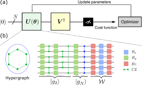
Figure 1: (a) Variational quantum algorithm (VQA) for quantum state preparation. To begin, we create the initial state $|\bm{0}\rangle$ and apply a series of $\bm{U}(\bm{\theta})$ followed by $\bm{V}^{\dagger}$. The resulting circuit is measured in $|\bm{0}\rangle\langle\bm{0}|$, and the outcome is sent to a classical computer for optimization and update new parameters to the quantum circuit. (b) The ansatz $\bm{U}(\bm{\theta})$ has a hypergraph-based structure, which includes the rotation gates $R_{j},j=\{x,y,z\}$ and the controlled-rotation-$Z$ gates (CZ).

II.2 Hypergraph-based ansatzes

A graph state is a configuration of multiple qubits that forms a graph structure with vertices and edges $\{V,E\}$. Each vertex represents a qubit and is connected to another qubit through an edge that uses a CZ gate for the interaction. In a regular graph state, every two qubits are connected in a pair:

$$|g_{2}\rangle=\prod_{\{i_{1},i_{2}\}\in E}{\rm CZ}_{i_{1}i_{2}}|+\rangle,$$ (5)

where two vertexes $i_{1},i_{2}$ connect via an edge, and $|+\rangle=(|0\rangle+|1\rangle)/\sqrt{2}$. A $k$-uniform hypergraph state is created in the same manner by connecting $k$ vertices with an edge, as described in Rossi et al. (2013)

$$|g_{k}\rangle=\prod_{\{i_{1},i_{2}\cdots i_{k}\}\in E}{\rm CZ}_{i_{1}i_{2}\cdots i_{k}}|+\rangle.$$ (6)

Studies have shown that graph and hypergraph states are entangled states Hein et al. (2004). For example, a star graph is equivalent to a GHZ state with a local unitary (LU) operation Hein et al. (2004); Dür et al. (2003), while a ring graph can be an AME state Cervera-Lierta et al. (2019). These states have practical applications in quantum error correction Liao et al. (2022); Looi et al. (2008); Hein et al. (2006), quantum computing Raussendorf and Briegel (2001); Nielsen (2006), quantum metrology Shettell and Markham (2020); Le et al. (2023), and other fields.

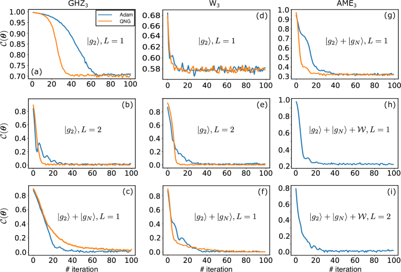
Figure 2: Cost function convergence for different target states and configuration ansatzes. For the GHZ and W target states, the ansatz $|g_{2}\rangle,L=1$ (a, d) fails to reach the global minimum, while increasing the ansatz depth to $L=2$ (b, e) or incorporating $|g_{N}\rangle$ configuration (c, f) enables reaching the global minimum. For the AME target, the ansatz $|g_{2}\rangle+|g_{N}\rangle,L=1$ (g) falls short of achieving the global minimum, but introducing the entangled term $\mathcal{W}$ improves the cost function (h) and leads to the global minimum (i). These results are shown for a system size of $N=3$ qubits.

This study uses hypergraph ansatzes to generate entangled states in quantum circuits. To create a graph-based ansatz, we use $R_{y}$ gates, with four $R_{y}$ gates surrounding each CZ gate. The formula for a single-qubit rotation is $R_{y}=\exp(-i\frac{\theta}{2}\sigma_{y})$, with $\sigma_{y}$ representing a Pauli matrix. This structure is similar to the one in Ref. Cerezo et al. (2021b). We focus on combining a ring 2-uniform graph $|g_{2}\rangle$ and an $N$-uniform hypergraph $|g_{N}\rangle$, where $N$ corresponds to the number of qubits. We also combine it with an entangled $\mathcal{W}$ ansatz for “phase” generation. For details, please refer to Fig. 1b. The circuit depth increases with the number of layers $L$, much smaller than sub-exponential. For a summary, please see Tab.  1 for a breakdown of these cases. Here, the circuit depth is determined by calculating the longest path between the data input and the output.

Table 1: Hypergraph-based ansatzes and their characteristics.

ansatz	$N$	# parameters	circuit depth
$|g_{2}\rangle$	even	$2NL$	$4L$
	odd		$6L$
$|g_{2}\rangle+|g_{N}\rangle$	even	$3NL$	$6L$
	odd		$8L$
$|g_{2}\rangle+|g_{N}\rangle+\mathcal{W}$	even	$6NL$	$9L$
	odd		$11L$

III Numerical Results

We conduct numerical simulation to train the variational model. We use the Qiskit open-source package (version 0.39.4), which is compatible with all platforms, to execute the simulation. To obtain the probability $p_{0}$ for each experiment, we run $10^{4}$ shots using the qasm simulator backend. The training process involves 100 iterations. Below we show the results of preparing some representative entangled states, including the GHZ, W, and AME states.

III.1 Cost function: case studies

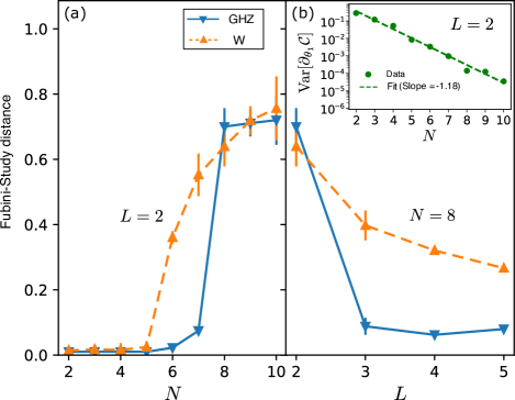
Figure 3: (a) Funibi-Study distance versus the number of qubits $N$ at $L=2$. We examine the target states GHZ and W. While the distance remains small up to $N=5$, then it increases when increasing $N$. (b) Fubini-Study distance versus the number of layers $L$ at $N=8$. For the GHZ target, the distance reaches the minimum at $L=4$, while for the W one, the distance continues to reduce. (inset): A semi-log plot of the variance ${\rm Var}[(\partial_{\theta_{1}}\mathcal{C})]$ as a function of $N$ at fixed $L=2$ and the GHZ target. As predicted, exponential decay is observed as proof of the existence of the barren plateaus. The slope of a fit line indicates the decay rate. In all cases, we use $|g_{2}\rangle$ ansatz and Adam optimizer.

In Fig. 2, we examine the cost function versus the number of iterations for different configurations. We fix $N=3$, and the target states are

$$|\psi\rangle_{\rm GHZ} =\dfrac{1}{\sqrt{2}}(|000\rangle+|111\rangle),$$ (7)

$$|\psi\rangle_{\rm W} =\dfrac{1}{\sqrt{3}}(|001\rangle+|010\rangle+|100\rangle),$$ (8)

$$|\psi\rangle_{\rm AME} =0.27|000\rangle+0.377|100\rangle+0.326|010\rangle$$

$$+0.363|001\rangle+0.74e^{-0.79i\pi}|111\rangle,$$ (9)

where the AME state is taken from Ref. Enríquez et al. (2016).

Figure 2(a-c) display results for the GHZ case. When using the ansatz $|g_{2}\rangle$ with $L=1$, the cost function $\mathcal{C}(\bm{\theta})$ reaches a local minimum of approximately 0.7 (Fig. 2a) due to the limited parameters space. However, at $L=2$, $\mathcal{C}(\bm{\theta})$ reaches the global minimum of zero (Fig. 2b). Similar outcomes are observed when using $|g_{2}\rangle+|g_{N}\rangle$ and maintaining $L=1$, as shown in Figure 2c. The results for the W case, as shown in Figs. 2(d-f), share similarities with the outcomes of the GHZ case. In the AME case, achieving the global minimum with $|g_{2}\rangle+|g_{N}\rangle,L=1$ configuration (Fig. 2g) is challenging because the AME state requires a higher degree of entanglement. To enhance the optimal outcomes, we incorporate an entangled term $\mathcal{W}$ into the hypergraph-based ansatz. The configuration $|g_{2}\rangle+|g_{N}\rangle+\mathcal{W}$ yields $\mathcal{C}(\bm{\theta})\approx 0.2$ with $L=1$ (Fig. 2h) and $\mathcal{C}(\bm{\theta})\approx 0.0$ with $L=2$ (Fig. 2i). Hence, the cost functions for all case studies presented here can attain the global minimum at a specific configuration. Upon comparing the Adam and QNG optimizers, it appears that the QNG optimizer reaches convergence in fewer iterations due to its superior ability to navigate toward the optimal direction Stokes et al. (2020); Haug and Kim (2021).

III.2 Funibi-Study distance vs $N$

In Fig. 3a, we present the numerical results for the Fubini-Study distance as a function of the number of qubits $N$. Specifically, we focus on $|g_{2}\rangle$ configuration with $L=2$, averaging the results over 10 repeated experiments using the Adam optimizer. Generally, the Fubini-Study distance tends to increase with the number of qubits, indicating lower accuracy in larger systems. However, in this analysis, we demonstrate that the Fubini-Study distance remains small, even up to $N=5$, suggesting high accuracy and stability within this range. Beyond $N=5$, the Fubini-Study distance gradually increases as $N$ increases. Moreover, preparing the target W state presents more significant challenges as it belongs to the multipartite entanglement class .

III.3 Funibi-Study distance vs $L$

The accuracy of the training process is significantly affected by the number of layers $L$ Steinbrecher et al. (2019); Torlai et al. (2020); Zhou et al. (2021). In Fig. 3b we demonstrate the correlation between the Fubini-Study distance and the number of layers using $|g_{2}\rangle$ ansatz with $N=8$ and the Adam optimizer. The Fubini-Study distance reaches its minimum at $L=4$ for the GHZ target and slightly increases when $L>4$. This observation aligns with the barren plateaus analyses depicted in the inset of Fig. 3 below. Concerning the W state, the distance decreases until $L=5$. This finding confirms the previous observation regarding the entangled characteristics of the GHZ and W classes, where achieving the same level of accuracy as the GHZ class requires a greater computational cost for preparing the W class.

III.4 Barren plateau

The results above indicate the presence of barren plateau effect (BP) in the training landscapes McClean et al. (2018), a phenomenon commonly observed in variational quantum algorithms and quantum neural networks. When the BP occurs, the derivative of the cost function $\mathcal{C}(\bm{\theta})$ exponentially diminishes with increasing circuit size McClean et al. (2018). The BP effect can arise from multiple factors, including random parameter initialization McClean et al. (2018), shallow depth with global cost functions Cerezo et al. (2021b), highly expressive ansatzes Holmes et al. (2022), entanglement-induced effects Ortiz Marrero et al. (2021), and noise-induced influences Wang et al. (2021a). Numerous strategies have been identified to bypass the BP effect, such as employing local cost functions Cerezo et al. (2021b); Uvarov and Biamonte (2021), utilizing correlated parameters Volkoff and Coles (2021), pretraining with classical neural networks Verdon et al. (2019), and adopting layer-by-layer training approaches Grant et al. (2019).

To investigate the disappearance of the derivative cost function $\mathcal{C}(\bm{\theta})$ and the presence of BP, we calculate the variance

$${\rm Var}[\partial_{k}\mathcal{C}]=\langle(\partial_{k}\mathcal{C})^{2}\rangle-\langle\partial_{k}\mathcal{C}\rangle^{2},$$ (10)

where we used $\mathcal{C}$ to represent $\mathcal{C}(\bm{\theta})$, $\partial_{k}\mathcal{C}$ to represent $\partial\mathcal{C}/\partial\theta_{k}$, and the expectation value is taken over the final state. The numerical result ${\rm Var}[\partial_{\theta_{1}}\mathcal{C}]$ for a representative first parameter $\theta_{1}$ is given in Fig. 3 inset. It demonstrates an exponential decay with a slope of -1.18 as the number of qubits $N$ increases. This is evidence for the existence of BP within the parameters space in our model and agrees with the prediction in main Fig. 3. The result is shown for the GHZ target and $L=2$.

III.5 Error mitigation

Finally, we consider the impact of noise and employ error mitigation techniques. In the current era of noisy intermediate-scale quantum computers (NISQ), the influence of noisy qubits induces biases and thus restricts the range of applications Nachman et al. (2020). One of the important classes of noisy qubits is the readout error, which typically arises from (i) qubits decoherence, i.e., qubits decay, phase change,…, during the measurement time, and (ii) incomplete measuring devices, i.e., the overlap between measured bases. Here we model the noise channel by a readout error probability for each qubit in the circuit as

$$\begin{pmatrix}p^{(\epsilon)}_{0}\\ p^{(\epsilon)}_{1}\end{pmatrix}=\begin{pmatrix}1-\epsilon&\epsilon\\ \epsilon&1-\epsilon\end{pmatrix}\begin{pmatrix}p_{0}\\ p_{1}\end{pmatrix},$$ (11)

where $p_{0},p_{1}$ are the true probabilities when measuring two elements $|0\rangle$ and $|1\rangle$ of the qubit, and $p^{(\epsilon)}_{0},p^{(\epsilon)}_{1}$ are the readout error probabilities, respectively, $\epsilon$ is the error rate.

In Fig. 4 (open circle, $\circ$), we observe a rapid increase in the Fubini-Study distance as the error rate rises. The inset of Fig. 4 displays the cost function for different $\epsilon$ values (the dotted lines), with rapid reduction and convergence around 100 iterations. However, for $\epsilon\in[0.01,0.04]$, the optimal values are limited to $[0.22,0.42]$. This results in an increased Fubini-Study distance in the main figure, leading to a loss of accuracy in the presence of noise.

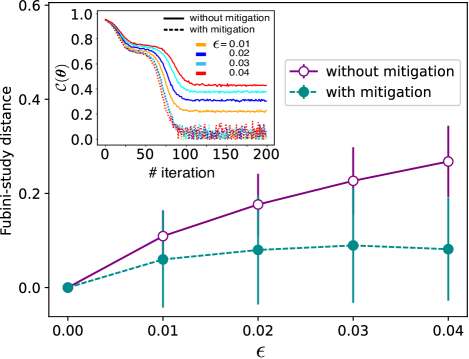
Figure 4: Fubini-Study distance under the presence of noise ($\epsilon$) with and without mitigation. Inset: plot of cost function versus iteration for two cases of with and without mitigation with various error rates $\epsilon$. We fixed $N=5,L=2$, QNG optimizer, and plot for $|g_{2}\rangle$ ansatz with the GHZ target.

To suppress the noise, we apply the measurement error mitigation technique Endo et al. (2021); Czarnik et al. (2021); Nation et al. (2021); Maciejewski et al. (2020). The basic ideal behind this method is to utilize a calibration matrix $\mathcal{M}$ of size $(2^{N}\times 2^{N})$, such that

$$\bm{p}^{(\epsilon)}=\mathcal{M}\bm{p},$$ (12)

where vector $\bm{p}=(p_{0},p_{1},\cdots,p_{2^{N}-1})^{\rm T}$ represents the true probabilities, and similar for $\bm{p}^{(\epsilon)}$ which represents the readout probabilities. The calibration matrix comprises all the transition probabilities, denoted a $\mathcal{M}_{ij}={\rm Prob}(p^{(\epsilon)}_{i}\to p_{j})$. An effective method to obtain the mitigated probabilities is inverting the calibration matrix, resulting in $\bm{p}^{\rm mitigated}=\mathcal{M}^{-1}\bm{p}^{(\epsilon)}$. Various techniques have been demonstrated, including the least square Geller (2020), truncated Neumann series Wang et al. (2021b), and unfolding methods Nachman et al. (2020). Here we limit ourselves to the direct approach which suffices for our analysis. We construct $\mathcal{M}$ by running $2^{N}$ circuits corresponding to $2^{N}$ elements in the computation basis $\{|00\cdots 0\rangle,|00\cdots 1\rangle,\cdots,|11\cdots 1\rangle\}$.

The mitigation results are depicted in Fig. 4 (filled circle, $\bullet$). In this specific instance, noise is effectively mitigated, leading to a significant reduction in the Fubini-Study distance, which becomes comparable to its original values before introducing noise. The average results are graphed after conducting 10 repeated experiments using the QNG optimizer.

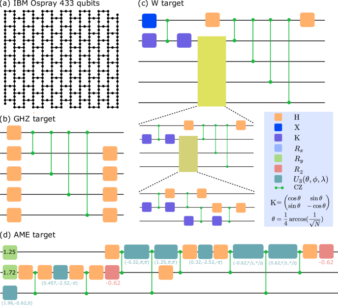
Figure 5: (a) The structure of IBM Osprey with 433 qubits, represented by dots, and the lines indicate their physical interaction. (b) The quantum circuit prepares the target GHZ state, with an example of $N=5$. (c) The quantum circuit prepares the target W state, with an example of $N=5$. (d) The quantum circuit prepares the target AME state, with an example of $N=3$.

IV Discussion

We emphasize two crucial advantages of the framework. Firstly, graph-based ansatzes exhibit high versatility and are compatible with the current superconductor-based quantum hardware architectures. For example, the IBM Osprey system, boasting 433 qubits, features a ring structure as depicted in Fig. 5a, where the nodes represent qubits, and the lines show their physical connections. In our approach, we can design graph-based ansatzes that align with this hardware’s vertices and edges, allowing for the utilization of various configurations such as linear, star, ring, and hypergraph ansatzes. This adaptability of variational ansatzes proves instrumental in effectively mitigating physical noise inherent in the system.

To prepare a GHZ state in quantum circuits, there are two approaches available. The first method directly utilizes the target unitary, as illustrated in Fig. 5b. However, this approach necessitates the interaction of at least one qubit with the remaining $N-1$ qubits, thereby restricting the preparation to cases where $N\leq 4$. On the other hand, employing a trainable ansatz with a ring structure can achieve comparable accuracy for any value of $N$, as illustrated in Fig. 3. However, as the value of $N$ increases, the worst-case scenarios may require a more significant number of layers, resulting in a deeper circuit configuration.

Another crucial aspect of our framework is the ability to reduce the circuit depth for trainable ansatzes. With this approach, the circuit depth remains constant regardless of the number of qubits $N$, enabling scalability. We have effectively demonstrated this scalability in the cases of W and AME, where the circuit depth of the trainable ansatzes is shorter than their respective target configurations (refer to Fig. 5(c, d) for the target unitaries of the W and AME states). Table 2 summarizes the circuit depth for $N$ up to 5, explicitly comparing cases where the trainable ansatzes successfully recover the target unitary, indecated by $\mathcal{C}(\bm{\theta})=0$.

Table 2: Comparison of circuit depth between target and trainable unitaries for $N$ ranging from 2 to 5.

$N$	2			3			4			5
	GHZ	W	AME	GHZ	W	AME	GHZ	W	AME	GHZ	W	AME
$|g_{2}\rangle,L=2$			-			-			-			-
$|g_{2}\rangle+|g_{N}\rangle,L=1$			-			-			-			-
$|g_{2}\rangle+|g_{N}\rangle+\mathcal{W},L=2$	-	-	-	-	-		-	-	-	-	-	-

V Conclusion

We presented a versatile variational algorithm for quantum state preparation that explicitly compiles a given quantum state to another. We thoroughly analyzed the algorithm’s performance through extensive numerical experiments using various hypergraph-based ansatzes and optimizers. Our algorithm offers the advantage of creating low-depth circuits, making it highly suitable for implementation on different quantum hardware platforms. Notably, it can be utilized for testing the capabilities of quantum hardware in various applications Cervera-Lierta et al. (2019).

Furthermore, we demonstrated the efficient preparation of entanglement classes and the effectiveness of employing an error mitigation protocol to suppress noise. This capability extends to any desired target state. Additionally, we explored the impact of the barren plateau phenomenon, an inherent consequence of expanding the system space.

Code availability: The codes used for this study are available in https://github.com/vutuanhai237/UC-VQA.

References

- de Leon et al. (2021) N. P. de Leon, K. M. Itoh, D. Kim, K. K. Mehta, T. E. Northup, H. Paik, B. S. Palmer, N. Samarth, S. Sangtawesin, and D. W. Steuerman, Science 372, eabb2823 (2021).
- Alexeev et al. (2021) Y. Alexeev, D. Bacon, K. R. Brown, R. Calderbank, L. D. Carr, F. T. Chong, B. DeMarco, D. Englund, E. Farhi, B. Fefferman, A. V. Gorshkov, A. Houck, J. Kim, S. Kimmel, M. Lange, S. Lloyd, M. D. Lukin, D. Maslov, P. Maunz, C. Monroe, J. Preskill, M. Roetteler, M. J. Savage, and J. Thompson, PRX Quantum 2, 017001 (2021).
- Ebadi et al. (2021) S. Ebadi, T. T. Wang, H. Levine, A. Keesling, G. Semeghini, A. Omran, D. Bluvstein, R. Samajdar, H. Pichler, W. W. Ho, S. Choi, S. Sachdev, M. Greiner, V. Vuletić, and M. D. Lukin, Nature 595, 227 (2021).
- Pirandola et al. (2015) S. Pirandola, J. Eisert, C. Weedbrook, A. Furusawa, and S. L. Braunstein, Nature Photonics 9, 641 (2015).
- Spiller (2003) T. P. Spiller, Materials Today 6, 30 (2003).
- Shor (1994) P. Shor, in Proceedings 35th Annual Symposium on Foundations of Computer Science (1994) pp. 124–134.
- Grover (1996) L. K. Grover, in Proceedings of the twenty-eighth annual ACM symposium on Theory of computing (1996) pp. 212–219.
- Harrow et al. (2009) A. W. Harrow, A. Hassidim, and S. Lloyd, Phys. Rev. Lett. 103, 150502 (2009).
- Xu et al. (2021) X. Xu, S. C. Benjamin, and X. Yuan, Phys. Rev. Applied 15, 034068 (2021).
- Lubasch et al. (2020) M. Lubasch, J. Joo, P. Moinier, M. Kiffner, and D. Jaksch, Phys. Rev. A 101, 010301 (2020).
- Preskill (2018) J. Preskill, Quantum 2, 79 (2018).
- Cerezo et al. (2021a) M. Cerezo, A. Arrasmith, R. Babbush, S. C. Benjamin, S. Endo, K. Fujii, J. R. McClean, K. Mitarai, X. Yuan, L. Cincio, and P. J. Coles, Nature Reviews Physics 3, 625 (2021a).
- Peruzzo et al. (2014) A. Peruzzo, J. McClean, P. Shadbolt, M.-H. Yung, X.-Q. Zhou, P. J. Love, A. Aspuru-Guzik, and J. L. O’Brien, Nature Communications 5, 4213 (2014).
- Nakanishi et al. (2019) K. M. Nakanishi, K. Mitarai, and K. Fujii, Phys. Rev. Research 1, 033062 (2019).
- Kirby et al. (2021) W. M. Kirby, A. Tranter, and P. J. Love, Quantum 5, 456 (2021).
- Gard et al. (2020) B. T. Gard, L. Zhu, G. S. Barron, N. J. Mayhall, S. E. Economou, and E. Barnes, npj Quantum Information 6, 10 (2020).
- Tkachenko et al. (2021) N. V. Tkachenko, J. Sud, Y. Zhang, S. Tretiak, P. M. Anisimov, A. T. Arrasmith, P. J. Coles, L. Cincio, and P. A. Dub, PRX Quantum 2, 020337 (2021).
- Zhou et al. (2020) L. Zhou, S.-T. Wang, S. Choi, H. Pichler, and M. D. Lukin, Phys. Rev. X 10, 021067 (2020).
- Arrasmith et al. (2019) A. Arrasmith, L. Cincio, A. T. Sornborger, W. H. Zurek, and P. J. Coles, Nature Communications 10, 3438 (2019).
- Kaubruegger et al. (2019) R. Kaubruegger, P. Silvi, C. Kokail, R. van Bijnen, A. M. Rey, J. Ye, A. M. Kaufman, and P. Zoller, Phys. Rev. Lett. 123, 260505 (2019).
- Koczor et al. (2020) B. Koczor, S. Endo, T. Jones, Y. Matsuzaki, and S. C. Benjamin, New Journal of Physics 22, 083038 (2020).
- Meyer et al. (2021) J. J. Meyer, J. Borregaard, and J. Eisert, npj Quantum Information 7, 89 (2021).
- Jones and Benjamin (2022) T. Jones and S. C. Benjamin, Quantum 6, 628 (2022).
- Volkoff et al. (2021) T. Volkoff, Z. Holmes, and A. Sornborger, PRX Quantum 2, 040327 (2021).
- Khatri et al. (2019) S. Khatri, R. LaRose, A. Poremba, L. Cincio, A. T. Sornborger, and P. J. Coles, Quantum 3, 140 (2019).
- Heya et al. (2018) K. Heya, Y. Suzuki, Y. Nakamura, and K. Fujii, arXiv preprint arXiv:1810.12745 (2018).
- Hai and Ho (2023) V. T. Hai and L. B. Ho, Scientific Reports 13, 3750 (2023).
- Aulicino et al. (2022) J. C. Aulicino, T. Keen, and B. Peng, International Journal of Quantum Chemistry 122, e26853 (2022).
- Ashhab (2022) S. Ashhab, Phys. Rev. Research 4, 013091 (2022).
- Kuzmin and Silvi (2020) V. V. Kuzmin and P. Silvi, Quantum 4, 290 (2020).
- Lvovsky and Raymer (2009) A. I. Lvovsky and M. G. Raymer, Reviews of modern physics 81, 299 (2009).
- D’Ariano et al. (2002) G. M. D’Ariano, M. De Laurentis, M. G. Paris, A. Porzio, and S. Solimeno, Journal of Optics B: Quantum and Semiclassical Optics 4, S127 (2002).
- Takeda et al. (2021) K. Takeda, A. Noiri, T. Nakajima, J. Yoneda, T. Kobayashi, and S. Tarucha, Nature Nanotechnology , 1 (2021).
- Möttönen et al. (2005) M. Möttönen, J. J. Vartiainen, V. Bergholm, and M. M. Salomaa, Quantum Info. Comput. 5, 467–473 (2005).
- Shende et al. (2006) V. Shende, S. Bullock, and I. Markov, IEEE Transactions on Computer-Aided Design of Integrated Circuits and Systems 25, 1000 (2006).
- Iten et al. (2016) R. Iten, R. Colbeck, I. Kukuljan, J. Home, and M. Christandl, Phys. Rev. A 93, 032318 (2016).
- Plesch and Brukner (2011) M. Plesch and i. c. v. Brukner, Phys. Rev. A 83, 032302 (2011).
- Sun et al. (2021) X. Sun, G. Tian, S. Yang, P. Yuan, and S. Zhang, “Asymptotically optimal circuit depth for quantum state preparation and general unitary synthesis,” (2021), arXiv:2108.06150 [quant-ph] .
- Zhang et al. (2021) X.-M. Zhang, M.-H. Yung, and X. Yuan, Phys. Rev. Research 3, 043200 (2021).
- Rosenthal (2022) G. Rosenthal, “Query and depth upper bounds for quantum unitaries via grover search,” (2022), arXiv:2111.07992 [quant-ph] .
- Araujo et al. (2021) I. F. Araujo, D. K. Park, F. Petruccione, and A. J. da Silva, Scientific Reports 11, 6329 (2021).
- Arrazola et al. (2019) J. M. Arrazola, T. R. Bromley, J. Izaac, C. R. Myers, K. Brádler, and N. Killoran, Quantum Science and Technology 4, 024004 (2019).
- Kuzmak (2021) A. R. Kuzmak, Quantum Information Processing 20, 269 (2021).
- Rossi et al. (2013) M. Rossi, M. Huber, D. Bruß, and C. Macchiavello, New Journal of Physics 15, 113022 (2013).
- Hein et al. (2004) M. Hein, J. Eisert, and H. J. Briegel, Phys. Rev. A 69, 062311 (2004).
- Dür et al. (2003) W. Dür, H. Aschauer, and H.-J. Briegel, Phys. Rev. Lett. 91, 107903 (2003).
- Cervera-Lierta et al. (2019) A. Cervera-Lierta, J. I. Latorre, and D. Goyeneche, Phys. Rev. A 100, 022342 (2019).
- Liao et al. (2022) P. Liao, B. C. Sanders, and D. L. Feder, Phys. Rev. A 105, 042418 (2022).
- Looi et al. (2008) S. Y. Looi, L. Yu, V. Gheorghiu, and R. B. Griffiths, Phys. Rev. A 78, 042303 (2008).
- Hein et al. (2006) M. Hein, W. Dür, J. Eisert, R. Raussendorf, M. V. den Nest, and H. J. Briegel, “Entanglement in graph states and its applications,” (2006), arXiv:quant-ph/0602096 [quant-ph] .
- Raussendorf and Briegel (2001) R. Raussendorf and H. J. Briegel, Phys. Rev. Lett. 86, 5188 (2001).
- Nielsen (2006) M. A. Nielsen, Reports on Mathematical Physics 57, 147 (2006).
- Shettell and Markham (2020) N. Shettell and D. Markham, Phys. Rev. Lett. 124, 110502 (2020).
- Le et al. (2023) T. K. Le, H. Q. Nguyen, and L. B. Ho, “Variational quantum metrology for multiparameter estimation under dephasing noise,” (2023), arXiv:2305.08289 [quant-ph] .
- Cerezo et al. (2021b) M. Cerezo, A. Sone, T. Volkoff, L. Cincio, and P. J. Coles, Nature Communications 12, 1791 (2021b).
- Enríquez et al. (2016) M. Enríquez, I. Wintrowicz, and K. Życzkowski, Journal of Physics: Conference Series 698, 012003 (2016).
- Stokes et al. (2020) J. Stokes, J. Izaac, N. Killoran, and G. Carleo, Quantum 4, 269 (2020).
- Haug and Kim (2021) T. Haug and M. Kim, arXiv preprint arXiv:2107.14063 (2021).
- Note (1) For W states, if one qubit is lost, the remaining system still entangles, from which contrasts with GHZ states, that fully separable after disentangling one qubit. See also Ref. PhysRevA.62.062314.
- Steinbrecher et al. (2019) G. R. Steinbrecher, J. P. Olson, D. Englund, and J. Carolan, npj Quantum Information 5, 60 (2019).
- Torlai et al. (2020) G. Torlai, C. J. Wood, A. Acharya, G. Carleo, J. Carrasquilla, and L. Aolita, “Quantum process tomography with unsupervised learning and tensor networks,” (2020), arXiv:2006.02424 [quant-ph] .
- Zhou et al. (2021) P.-F. Zhou, R. Hong, and S.-J. Ran, Phys. Rev. A 104, 042601 (2021).
- McClean et al. (2018) J. R. McClean, S. Boixo, V. N. Smelyanskiy, R. Babbush, and H. Neven, Nature Communications 9, 4812 (2018).
- Holmes et al. (2022) Z. Holmes, K. Sharma, M. Cerezo, and P. J. Coles, PRX Quantum 3, 010313 (2022).
- Ortiz Marrero et al. (2021) C. Ortiz Marrero, M. Kieferová, and N. Wiebe, PRX Quantum 2, 040316 (2021).
- Wang et al. (2021a) S. Wang, E. Fontana, M. Cerezo, K. Sharma, A. Sone, L. Cincio, and P. J. Coles, Nature Communications 12, 6961 (2021a).
- Uvarov and Biamonte (2021) A. V. Uvarov and J. D. Biamonte, Journal of Physics A: Mathematical and Theoretical 54, 245301 (2021).
- Volkoff and Coles (2021) T. Volkoff and P. J. Coles, Quantum Science and Technology 6, 025008 (2021).
- Verdon et al. (2019) G. Verdon, M. Broughton, J. R. McClean, K. J. Sung, R. Babbush, Z. Jiang, H. Neven, and M. Mohseni, arXiv preprint arXiv:1907.05415 (2019).
- Grant et al. (2019) E. Grant, L. Wossnig, M. Ostaszewski, and M. Benedetti, Quantum 3, 214 (2019).
- Nachman et al. (2020) B. Nachman, M. Urbanek, W. A. de Jong, and C. W. Bauer, npj Quantum Information 6, 84 (2020).
- Endo et al. (2021) S. Endo, Z. Cai, S. C. Benjamin, and X. Yuan, Journal of the Physical Society of Japan 90, 032001 (2021), https://doi.org/10.7566/JPSJ.90.032001 .
- Czarnik et al. (2021) P. Czarnik, A. Arrasmith, P. J. Coles, and L. Cincio, Quantum 5, 592 (2021).
- Nation et al. (2021) P. D. Nation, H. Kang, N. Sundaresan, and J. M. Gambetta, PRX Quantum 2, 040326 (2021).
- Maciejewski et al. (2020) F. B. Maciejewski, Z. Zimborás, and M. Oszmaniec, Quantum 4, 257 (2020).
- Geller (2020) M. R. Geller, Quantum Science and Technology 5, 03LT01 (2020).
- Wang et al. (2021b) K. Wang, Y.-A. Chen, and X. Wang, arXiv preprint arXiv:2103.13856 (2021b).