Screw and Lie Group Theory in Multibody Kinematics

Abstract

After three decades of computational multibody system (MBS) dynamics, current research is centered at the development of compact and user friendly yet computationally efficient formulations for the analysis of complex MBS. The key to this is a holistic geometric approach to the kinematics modeling observing that the general motion of rigid bodies as well as the relative motion due to technical joints are screw motions. Moreover, screw theory provides the geometric setting and Lie group theory the analytic foundation for an intuitive and compact MBS modeling. The inherent frame invariance of this modeling approach gives rise to very efficient recursive $O\left(n\right)$ algorithms, for which the so-called ’spatial operator algebra’ is one example, and allows for use of readily available geometric data. In this paper three variants for describing the configuration of tree-topology MBS in terms of relative coordinates, i.e. joint variables, are presented: the standard formulation using body-fixed joint frames, a formulation without joint frames, and a formulation without either joint or body-fixed reference frames. This allows for describing the MBS kinematics without introducing joint reference frames and therewith rendering the use of restrictive modeling convention, such as Denavit-Hartenberg parameters, redundant. Four different definitions of twists are recalled and the corresponding recursive expressions are derived. The corresponding Jacobians and their factorization are derived. The aim of this paper is to motivate the use of Lie group modeling and to provide a review of the different formulations for the kinematics of tree-topology MBS in terms of relative (joint) coordinates from the unifying perspective of screw and Lie group theory.

1 Introduction

Computational multibody system (MBS) dynamics aims at mathematical formulations and efficient computational algorithms for the kinetic analysis of complex mechanical systems. At the same time the modeling process is supposed to be intuitive and user friendly. Moreover, the efficiency of MBS algorithms as well as the complexity of the actual modeling process is largely determined by the way in which the kinematics is described. This concerns the core issues of representing rigid body motions and of describing the kinematics of technical joints. Both issues can be addressed with concepts of screw and Lie group theory.

Spatial MBS perform complicated motions, and in general rigid bodies perform screw motions that form a Lie group. Although the theory of screw motions is well understood, screw theory has almost completely been ignored for MBS modeling with only a few exceptions. The latter can be grouped into two classes. The first class makes use of the fact that the velocity of a rigid body is a screw, referred to as the twist. The propagation of twists within an MBS is thus described as a frame transformation of screw coordinates. This gave rise to the so-called ’spatial vector’ formulation introduced in Featherstone1983 ; Featherstone2008 , and to the so-called ’spatial operator algebra’ that was formalized in Rodriguez1991 and used for $O\left(n\right)$ forward dynamics algorithms e.g. in Fijany1995 ; Jian1991 ; Jian1995 ; LillyOrin1991 ; Rodriguez1987 ; Rodriguez1992 . Screw notations are also used in the formulations presented in Angeles2003 ; Legnani1 ; Legnani2 ; Uicker2013 . Further MBS formulations were reported that use screw notations uncommon for the MBS community Gallardo2003 . All these approaches only exploit the algebraic properties of screws as far as relevant for a compact handling of velocities, accelerations, wrenches, and inertia. The second class goes one step further by recognizing that finite motions form the Lie group $SE\left(3\right)$ with the screw algebra as its Lie algebra $se\left(3\right)$. Moreover, screw theory provides the geometric setting and Lie group theory the analytic foundation for an intuitive and efficient modeling of rigid body mechanisms. Some of the first publications reporting Lie group formulations of the kinematics of an open kinematic chain are Brockett1984 ; Hervet1978 ; Hervet1982 and Chevalier1991 ; Chevalier1994 . In this context the term product of exponentials (POE) is being used since Brockett used it in Brockett1984 . Unfortunately these publications have not reached the MBS community, presumably because of the used mathematical concepts that differ from classical MBS formalisms. The basic concept is the exponential mapping that determines the finite relative motion of two adjacent bodies connected by a lower pair joint in terms of a screw associated with the joint. The product of the exponential mappings for all consecutive joints determines the overall motion of the chain. Within this formulation twists are naturally represented as screws, and joint motions are described in terms of screw coordinates.

Motivated by Brockett1984 Lie group formulations for MBS dynamics were reported in a few publications, e.g. Mladenova2006 ; MUBOLieGroup ; Park1994 ; ParkBobrowPloen1995 ; PloenPark1997 ; PloenPark1999 ; ParkKim2000 . It should be mentioned that the basic elements of a screw formulation for MBS dynamics were already presented in Liu1988 , but did not receive due attention.

A crucial feature of these geometric approaches is their frame invariance, which allows for arbitrary representations of screws and for freely assigning reference frames, which drastically simplify the kinematics modeling and also provides a direct link to CAD models. Moreover, the POE, and thus the kinematics, can even be formulated without the use of any joint frame, which basically resembles the ’zero reference’ formulation that was reported for a robotic arm in Gupta1986 . On the other hand, classical approaches to the description of joint kinematics are the Denavit-Hartenberg (DH) DenavitHartenberg1955 ; KhalilKleinfinger1986 (in its different forms) and the Sheth-Uicker two-frame convention ShethUicker1971 . Such two-frame conventions are used in most of the current MBS dynamics simulations packages that use relative coordinates. The Lie group description, on the other hand, not only allows for arbitrary placement of joint frames but makes them dispensable altogether.

The benefits of geometric modeling have been recognized already in robotics. Recently, at least in robotics, the text books LynchPark2017 ; Murray ; Selig have reached a wider audience. Modern approaches to robotics make extensive use of screw and Lie group theoretical concepts. This is, also supported by the Universal Robot Description Format (URDF) that is used for instance in the Robot Operating System (ROS), rather than DH parameters. In MBS dynamics the benefits of geometric mechanics are slowly being recognized. Interestingly, this mainly applies to the modeling of MBS with flexible bodies undergoing large deformations Bauchau2011 ; Sonneville2014 . This is not surprising since geometrically exact formulations require correct modeling of the finite kinematics of a continua. The displacement field of a Cosserat beam, for instance, is a proper motion in $E^{3}$ and thus modeled as motion in $SE\left(3\right)$. This is an extension of the original work on geometrically exact beams and shells by Simo Simo1986 ; Simo1991 where the displacement field is modeled on $SO\left(3\right)\times{\mathbb{R}}^{3}$. Another topic where Lie group theory is recently applied in MBS dynamics is the time integration. To this end, Lie group integration schemes were modified and applied to MBS models in absolute coordinate formulation BruelsCardonaArnold2012 , where the motion of individual bodies is described as a general screw motion that are constrained according to the interconnecting joints. It shall be remarked that, despite the current trend to emphasize the use of Lie group (basic) concepts, the basics formulations for non-linear flexible MBS were already reported by Borri et al., e.g. Borri2001a ; Borri2001b ; Borri2003 .

The aim of this paper is to provide a comprehensive summary of the basic concepts for modeling MBS in terms of relative coordinates using joint screws and to relate them to existing formulations that are scattered throughout the literature. Without loss of generality the concepts are introduced for a kinematic chain within a MBS with arbitrary topology Abhi2011a ; Topology . It is also the aim to show that MBS can be modeled in a user-friendly way without having to follow restrictive modeling conventions, and that this gives rise to $O\left(n\right)$ formulations. The latter are not the topic of this paper.

The paper is organized as follows. In section 2 the MBS configuration is described in terms of joint variables, used as generalized coordinates, with the joint geometry parameterized by joint screw coordinates. This classical approach of using body-fixed joint frames to describe relative configurations is extended to a formulation that does not involve joint frames. The corresponding relations for the MBS velocity are derived in section 3. A formulation is introduced for each of the four different definitions of rigid body twists found in the literature. The latter are called the body-fixed, spatial, hybrid, and mixed twists. They differ by the reference point used to measure the velocity and by the frame in which the angular and translational velocities are resolved. The different twist representations are introduced in appendix A.2. Recursive relations for the respective Jacobians are derived, and the computational aspects are discussed with emphasize on their decomposition. The presented formulation allows for an efficient modeling of the MBS kinematics in terms of readily available geometric data. Throughout the paper only a few basic concepts from Lie group theory are required that are summarized in appendix A. The used nomenclature is summarized in appendix B.

As for all Lie group formulations the biggest hurdle for a reader (who may be already be familiar with MBS formulations) is the notation. The reader not familiar with screws and Lie group modeling may want to consult the appendix A.1 before reading section 2 and appendix A.2 before reading section 3. This paper is aimed to provide a reference and cannot replace an introductory textbook like LynchPark2017 ; Murray ; Selig . A beginner is recommended to consult LynchPark2017 . Yet there is no text book that treats the topic from a MBS perspective. Readers not interested in the derivations could simply use the main relations that are displayed with a black border.

2 Configuration of a Kinematic Chain

In this section the kinematics modeling using joint screw coordinates is presented. For simplicity a single open kinematic chain is considered comprising $n$ moving bodies interconnected by $n$ 1-DOF lower pair joints. To simplify the formulation, but without loosing generality, higher-DOF joints are modeled as combination of 1-DOF lower pair joints. Bodies and joints are labeled with the same indices $i=1,\ldots,n$ while the ground is indexed with 0. With the sequential numbering of bodies and joints of the kinematic chain, joint $i$ connects body $i$ to its predecessor body $i-1$. A body-fixed reference frame (BFR) $\mathcal{F}_{i}$ is attached to body $i$ of the MBS. The body is then kinematically represented by this BFR.

2.1 Joint Kinematics

It has been the standard approach in MBS modeling to represent higher-DOF joints by combination of 1-DOF lower pair joints, i.e. using either revolute, prismatic, or screw joints. This will be adopted in the following although this is not the way in which MBS models are implemented in practice, but it simplifies the introduction of the presented approach without compromising its generality. The justification of this approach is that most technical joints are so-called lower kinematic pairs (also called Reuleaux pairs) characterized by surface contact Reuleaux1875 ; Reuleaux1963 . That is, they are the mechanical generators of motion subgroups of $SE\left(3\right)$ Selig . But not all motion subgroups are generated by lower pairs. The 10 subgroups are listed in table 1. So-called ’macro joints’ are frequently used in MBS modeling to generate motion subgroups by combination of lower pairs. Table 2 shows the correspondence of motion subgroups with lower pairs and macro joints. Missing in this list are joints relevant for MBS modeling such as universal/hook and constant velocity joints since they are not lower kinematic pairs. They can be modeled by combination of lower pair joints.

$n$	Subgroup	Motion
1	$\mathbb{R}$	1-dim. translation along some axis
1	$SO\left(2\right)$	1-dim. rotation about arbitrary fixed axis
1	$H_{p}$	screw motion about arbitrary axis with finite pitch
2	$\mathbb{R}^{2}$	2-dim. planar translation
2	$SO\left(2\right)\ltimes\mathbb{R}$	translation along arbitrary axis & rotation along this axis
3	$\mathbb{R}^{3}$	spatial translations
3	$SO\left(3\right)$	spatial rotations about arbitrary fixed point
3	$H_{p}\ltimes\mathbb{R}^{2}$	translation in a plane + screw motion $\bot$ to this plane (pitch $h$)
3	$SO\left(2\right)\ltimes\mathbb{R}^{2}=SE\left(2\right)$	planar motions
4	$SO\left(2\right)\ltimes\mathbb{R}^{3}=SE\left(2\right)\ltimes\mathbb{R}$	spatial translations + rotation about axis with fixed orientation
		(Schönflies motion)
6	$SE\left(3\right)$	spatial motion

Table 1: $n$-dimensional motion subgroups of $SE(3)$.

$n$	Subgroup	Lower Pair	Macro Joint
1	$\mathbb{R}$	Prismatic Joint	$\times$
1	$SO\left(2\right)$	Revolute Joint	$\times$
1	$H_{p}$	Screw Joint	$\times$
2	$\mathbb{R}^{2}$	$\times$	combination of two non-parallel
			prismatic joints
2	$SO\left(2\right)\ltimes\mathbb{R}$	Cylindrical Joint	$\times$
3	$\mathbb{R}^{3}$	$\times$	combination of three non-parallel
			prismatic joints
3	$SO\left(3\right)$	Spherical Joint	$\times$
3	$H_{p}\ltimes\mathbb{R}^{2}$	$\times$	planar joint + screw joint with axis
			normal to plane
3	$SO\left(2\right)\ltimes\mathbb{R}^{2}=SE\left(2\right)$	Planar Joint	$\times$
4	$SO\left(2\right)\ltimes\mathbb{R}^{3}=SE\left(2\right)\ltimes\mathbb{R}$	$\times$	planar joint + prismatic joint
			with axis normal to plane
6	$SE\left(3\right)$	$\times$	’free joint’

Table 2: Mechanical generators of the $n$-dimensional subgroups of $SE(3)$. A motion subgroup can be generated by a lower pair or by a ’macro joint’, i.e. a combination of joints with smaller DOF.

The classical approach to describe joint kinematics is to introduce an additional pair of body-fixed joint frames (JFR) for each joint (fig. 1) Uicker2013 . Denote with $\mathcal{J}_{i-1,i}$ the JFR for joint $i$ on body $i-1$ and with $\mathcal{J}_{i,i}$ the JFR on body $i$. The relative motion of adjacent bodies is represented by the frame transformation between the respective JFRs that can be described in terms of screw coordinates (appendix A.1).

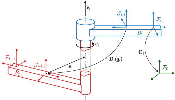
Figure 1: Description of the kinematics of joint $i$ connecting body $i$ with its predecessor body $i-1$. A body-fixed JFR $\mathcal{J}_{i,i}$ is introduced on body $i$, and $\mathcal{J}_{i-1,i}$, on body $i-1$, respectively. A revolute joint is shown as example.

Lower pair 1-DOF joints restrict the interconnected bodies so to perform screw motions with a certain pitch $h$. Revolute joints have pitch $h=0$, and prismatic joints $h=\infty$, while proper screw joints have a non-zero finite pitch. Denote with

$${{}^{i-1}}\mathbf{Z}_{i}=\left(\begin{array}[]{c}{{}^{i-1}}\mathbf{e}{{}_{i}}\\ {{}^{i-1}}\mathbf{z}{{}_{i}}\times{{}^{i-1}}\mathbf{e}{{}_{i}}+{{}^{i-1}}\mathbf{e}{{}_{i}h}_{i}\end{array}\right)$$ (1)

the unit screw coordinate vector of joint $i$ expressed in the JFR $\mathcal{J}_{i-1,i}$ on body $i-1$, where ${{}^{i-1}}\mathbf{z}{{}_{i}}$ is the position vector of a point on the joint axis measured in the JFR $\mathcal{J}_{i-1,i}$, and ${{}^{i-1}}\mathbf{e}{{}_{i}}$ is the unit vector along the joint axis resolved in JFR $\mathcal{J}_{i-1,i}$.

It is assumed throughout the paper that the two JFRs coincide in the reference configuration $q_{i}=0$. This assumption can be easily relaxed if required.

Denote with $q_{i}$ the joint variable (angle, translation). With the above assumption the configuration of the JFR $\mathcal{J}_{i,i}$ on body $i$ relative to the JFR $\mathcal{J}_{i-1,i}$ on body $i-1$ is given by the exponential in (85) as $\mathbf{D}_{i}\left(q_{i}\right):=\exp({}{}{{}^{i-1}}\mathbf{Z}_{i}q_{i})$.

Remark 1

It is common practice to locate the JFRs with their origins at the joint axis (as in Fig. 2), so that $\mathbf{z}=\mathbf{0}$. Then the joint screw coordinates for the three types of 1-DOF joints are

$$\mathbf{Z}^{\text{revolute}}=\left(\begin{array}[]{c}\mathbf{e}\\ \mathbf{0}\end{array}\right),\ \mathbf{Z}^{\text{screw}}=\left(\begin{array}[]{c}\mathbf{e}\\ \mathbf{e}{h}\end{array}\right),\ \mathbf{Z}^{\text{prismatic}}=\left(\begin{array}[]{c}\mathbf{0}\\ \mathbf{e}\end{array}\right).$$ (2)

2.2 Recursive Kinematics using Body-Fixed Joint Frames

The absolute configuration of body $i$, i.e. the configuration of its BFR $\mathcal{F}_{i}$ relative to the inertial frame (IFR) $\mathcal{F}_{0}$, is represented by $\mathbf{C}_{i}\in SE\left(3\right)$. The relative configuration of body $i$ relative to body $i-1$ is $\mathbf{C}_{i-1,i}:=\mathbf{C}_{i-1}^{-1}\mathbf{C}_{i}$. The configuration of a rigid body in the kinematic chain can be determined recursively by successive combination of the relative configurations of adjacent bodies as $\mathbf{C}_{i}=\mathbf{C}_{0,1}\mathbf{C}_{1,2}\cdots\mathbf{C}_{i-1,i}$.

For joint $i$ denote with ${}\mathbf{S}_{i-1,i}$ the constant transformation from JFR $\mathcal{J}_{i-1,i}$ to the RFR $\mathcal{F}_{i-1}$ on body $i-1$, and with $\mathbf{S}_{i,i}$ the constant transformation from JFR $\mathcal{J}_{i,i}$ to the RFR $\mathcal{F}_{i}$ on body $i$ (fig. 2). The relative configuration is then $\mathbf{C}_{i-1,i}={}\mathbf{S}_{i-1,i}\mathbf{D}_{i}\left(q_{i}\right){}\mathbf{S}_{i,i}^{-1}$. Denote with $\mathbf{q}\in{\mathbb{V}}^{n}$ the vector of joint variables that serve as generalized coordinates of the MBS. The joint space manifold is ${\mathbb{V}}^{n}={\mathbb{R}}^{n_{\text{P}}}\times\mathbb{T}^{n_{\text{R}}}$ for an MBS model comprising $n_{\text{P}}$ prismatic and $n_{\text{R}}$ revolute/screw joints ($n_{\text{P}}+n_{\text{R}}=n$).

The absolute configuration (i.e. relative to the IFR) of body $i$ in the chain is

$$\mathbf{C}_{i}\left(\mathbf{q}\right)=\mathbf{S}_{0,1}\mathbf{D}_{1}\left(q_{1}\right)\mathbf{S}_{1,1}^{-1}\cdot\mathbf{S}_{1,2}\mathbf{D}_{2}\left(q_{2}\right)\mathbf{S}_{2,2}^{-1}\cdot\ldots\cdot\mathbf{S}_{i-1,i}\mathbf{D}_{i}\left(q_{i}\right)\mathbf{S}_{i,i}^{-1}.$$

(3)

This formulation requires the following modeling steps:

• Introduction of body-fixed JFR $\mathcal{J}_{i,i}$ at body $i$ with relative configuration $\mathbf{S}_{i,i}$,

• Introduction of body-fixed JFR $\mathcal{J}_{i-1,i}$ at body $i-1$ with relative configurations $\mathbf{S}_{i-1,i}$,

• The screw coordinate vector ${{}^{i-1}}\mathbf{Z}_{i}$ of joint $i$ represented in JFR $\mathcal{J}_{i-1,i}$ at body $i-1$.

The expression (3) is the standard MBS formulation for the kinematics of an open chain in terms of relative coordinates, i.e. joint angles or translations. For 1-DOF joints the JFR is usually oriented such that its 3-axis points along the joint axis (as in figure 2). The screw coordinates are then ${{}^{i-1}}\mathbf{Z}_{i}=(0,0,1-s_{i},0,0,s_{i}+h_{i}\left(1-s_{i}\right))^{T}$ where $s_{i}\,=1$ for prismatic joint, and $s_{i}=0$ for a screw joint with finite pitch $h_{i}$ (for revolute joints $h_{i}=0$).

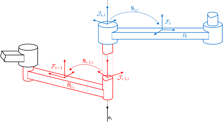
Figure 2: Definition of body-fixed RFR $\mathcal{F}_{i}$ and JFR $\mathcal{J}_{i,i}$ and $\mathcal{J}_{i-1,i}$, for joint $i$.

Remark 2

The matrix $\mathbf{C}_{i}$ is used to represent the configuration of body $i$; hence the symbol. Frequently the symbol $\mathbf{T}_{i}$ is used LynchPark2017 ; Uicker2013 , which refers to the fact that these matrices describe the transformation of point coordinates (appendix A.1)

Remark 3

It is important to emphasize that the Lie group formulation (3) is merely another approach to the standard matrix formulation of MBS kinematics aiming at compact expressions that simplify the implementation without compromising the efficiency. It also includes the various conventions used to describe the joint kinematics. An excellent overview of classical matrix methods (also with emphasis on how they can be employed for synthesis) can be found in Uicker2013 . For instance, $\mathbf{S}_{i-1,i}$ and $\mathbf{S}_{i,i}$ can be parameterized in terms of the constant part of the Denavit-Hartenberg (DH) parameters Uicker2013 . The formulation (3) in particular resembles the Sheth-Uicker convention (that was introduced to eliminate the ambiguity of DH parameter) ShethUicker1971 ; Uicker2013 . In that notation the matrices $\mathbf{S}_{i-1,i}$ and $\mathbf{S}_{i,i}$ are called the shape matrices of joint $i$. However, the Sheth-Uicker convention still presumes certain alignment of joint axes. E.g. a revolute axis is supposed to be parallel to the 3-axis of the JFRs. A recent discussion of these notations can be found in BongardtPhD . An expression similar to (3) was also presented in Orin1979 where no restriction on the joint axis is imposed. A recursive formulation of the MBS motion equations using homogeneous transformation matrices was also presented in Legnani1 ; Legnani2 .

Remark 4 (Multi-DOF joints)

The description for 1-DOF joints in terms of a screw coordinate vector $\mathbf{Z}_{i}$ can be generalized to joints with more than one DOF. For a joint with DOF $\nu$ the relative configuration of the JFRs can alternatively be described in terms of $\nu$ joint variables $q_{i_{1}},\ldots,q_{i_{\nu}}$ by $\mathbf{D}_{i}\left(q_{i_{1}},\ldots,q_{i_{\nu}}\right):=\exp({}{}{{}^{i-1}}\mathbf{Z}_{i_{1}}q_{i_{1}}+\ldots+{{}^{i-1}}\mathbf{Z}_{i_{\nu}}q_{i_{\nu}})$ or $\mathbf{D}_{i}\left(q_{i_{1}},\ldots,q_{i_{\nu}}\right):=\exp({}{}{{}^{i-1}}\mathbf{Z}_{i_{1}}q_{i_{1}})\cdot\ldots\cdot\exp({}{}{{}^{i-1}}\mathbf{Z}_{i_{\nu}}q_{i_{\nu}})$. For a spherical joint, for instance, the variables in the first form are the components of the rotation axis times angle in (80), and in the second form these are three angles corresponding to the order of 1-DOF rotations (e.g. Euler-angles). For lower pair joints, in the first case, $q_{i_{1}},\ldots,q_{i_{\nu}}$ are canonical coordinates of first kind on the joint’s motion subgroup, and in the second case they are canonical coordinates of second kind Murray . The $\mathbf{Z}_{i_{1}},\ldots,\mathbf{Z}_{i_{\nu}}$ form a basis on the subalgebra of the motion subgroup generated by the joint.

2.3 Recursive Kinematics without Body-Fixed Joint Frames

The introduction of joint frames is a tedious step within the MBS kinematics modeling. Moreover, it is desirable to minimize the data required to formulate the kinematic relations. In this regard the frame invariance of screws is beneficial.

The two constant transformations from the JFR to the BFR on the respective body can be summarized using (92) as

$$\mathbf{C}_{i-1,i}\left(q_{i}\right)=\mathbf{S}_{i-1,i}\mathbf{D}_{i}\left(q_{i}\right)\mathbf{S}_{i,i}^{-1}=\mathbf{S}_{i-1,1}\mathbf{S}_{i,i}^{-1}\mathbf{S}_{i,i}\mathbf{D}_{i}\left(q_{i}\right)\mathbf{S}_{i,i}^{-1}=\mathbf{B}_{i}\exp({{}^{i}}\mathbf{X}_{i}q_{i})$$ (4)

so that the relative configuration splits into only one constant and a variable part. The constant part $\mathbf{B}_{i}:=\mathbf{S}_{i-1,i}\mathbf{S}_{i,i}^{-1}=\mathbf{C}_{i-1,i}\left(0\right)$ is the reference configuration of body $i$ w.r.t. body $i-1$ when $q_{i}=0$. The variable part is now given in terms of the constant screw coordinate vector of joint $i$ represented in BFR $\mathcal{F}_{i}$

$${{}^{i}}\mathbf{X}_{i}=\mathbf{Ad}_{\mathbf{S}_{i,i}}{{}^{i-1}}\mathbf{Z}_{i}=\left(\begin{array}[]{c}{{}^{i}}\mathbf{e}_{i}\\ {{}^{i}}\mathbf{x}_{i,i}\times{{}^{i}}\mathbf{e}_{i}+h_{i}{{}^{i}}\mathbf{e}_{i}\end{array}\right).$$ (5)

The matrix $\mathbf{Ad}_{\mathbf{S}_{i,i}}$, defined in (89), transforms screw coordinates represented in $\mathcal{J}_{i,i-1}$ to those represented in $\mathcal{F}_{i}$ according to their relative configuration described by $\mathbf{S}_{i,i}$.

As indicated in fig. 3, here ${{}^{i}}\mathbf{e}_{i}$ is the unit vector along the axis of joint $i$ resolved in the BFR $\mathcal{F}_{i}$, and ${{}^{i}}\mathbf{x}_{i,i}$ is the position vector of a point on the axis of joint $i$, measured and resolved in $\mathcal{F}_{i}$. This is indeed the same screw as in (1) but expressed in the BFR on body $i$.

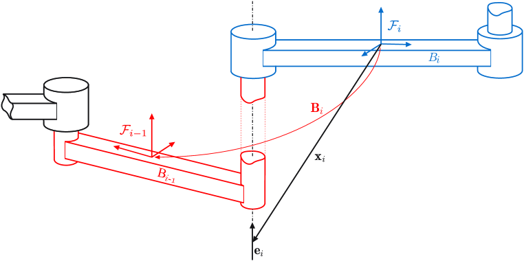
Figure 3: Description of the kinematics of joint $i$ without body-fixed JFRs, in the zero-reference relative configuration with $q_{i}=0$. The vector $\mathbf{x}_{i}$ is used when the joint screw coordinates are represented in the BFR $\mathcal{F}_{i}$ on body $i$, and $\bar{\mathbf{x}}_{i-1,i}$ is used when the joint screw coordinates are represented in the BFR $\mathcal{F}_{i-1}$ on body $i-1$.

The joint screw can alternatively be represented in $\mathcal{F}_{i-1}$. Then

$$\mathbf{C}_{i-1,i}\left(q_{i}\right)=\mathbf{S}_{i,i-1}\mathbf{D}_{i}\left(q_{i}\right)\mathbf{S}_{i,i}^{-1}=\mathbf{S}_{i,i-1}\mathbf{D}_{i}\left(q_{i}\right)\mathbf{S}_{i,i-1}^{-1}\mathbf{S}_{i,i-1}\mathbf{S}_{i,i}^{-1}=\exp({{}^{i-1}}\bar{\mathbf{X}}_{i}q_{i})\mathbf{B}_{i}$$ (6)

with the joint screw coordinate vector

$${{}^{i-1}}\bar{\mathbf{X}}_{i}=\mathbf{Ad}_{\mathbf{S}_{i-1,i}}{{}^{i-1}}\mathbf{Z}_{i}=\mathbf{Ad}_{\mathbf{B}_{i}}{{}^{i}}\mathbf{X}_{i}=\left(\begin{array}[]{c}{{}^{i-1}}\mathbf{e}_{i}\\ {{}^{i-1}}\bar{\mathbf{x}}_{i-1,i}\times{{}^{i-1}}\mathbf{e}_{i}+{{}^{i-1}}\mathbf{e}_{i}h_{i}\end{array}\right)$$ (7)

now expressed in the BFR $\mathcal{F}_{i-1}$ at body $i-1$, where ${{}^{i-1}}\bar{\mathbf{x}}_{i-1,i}$ is the position vector of a point on the axis of joint $i$ measured in $\mathcal{F}_{i-1}$.

Successive combination of the relative configurations yields

$$\mathbf{C}_{i}\left(\mathbf{q}\right)$$

(8)

The first form of (8) was reported PloenPark1999 , and both forms in Park1994 ; ParkBobrowPloen1995 . It will be called the body-fixed Product-of-Exponentials (POE) formula in body-fixed description since the joint kinematics is expressed by exponentials of joint screws. It seems to be more convenient to work with the screw coordinates ${{}^{i}}\mathbf{X}_{i}$. Also in Angeles2003 two variants of the kinematic description of a serial chain were presented using a BFR on body $i-1$ or $i$, respectively.

In summary this body-fixed POE formulation does not require introduction of JFRs. It only requires the following readily available information:

• The relative reference configuration $\mathbf{B}_{i}$ of the adjacent bodies connected by joint $i$ for $q_{i}=0$,

• The screw coordinates ${{}^{i}}\mathbf{X}_{i}$ of joint $i$ represented in the BFR $\mathcal{F}_{i}$ at body $i$, or alternatively the screw coordinates ${{}^{i-1}}\bar{\mathbf{X}}_{i}$ represented in the BFR $\mathcal{F}_{i-1}$ at body $i-1$.

The form (8) simplifies the expression for the joint kinematics. Its main advantage is that it only involves the reference configuration $\mathbf{B}_{i}$ of BFRs.

2.4 Recursive Kinematics without Body-Fixed Joint Frames and Screw Coordinates

Thanks to the frame invariance, the joint screw coordinates can even be described in the spatial IFR, i.e. without reference to any body-fixed frames. To this end, (8) is written as

$$\mathbf{C}_{i}\left(\mathbf{q}\right) = \mathbf{B}_{1}\exp({{}^{1}}\mathbf{X}_{1}q_{1})\mathbf{B}_{1}^{-1}\cdot$$

$$\mathbf{B}_{1}\mathbf{B}_{2}\exp({{}^{2}}\mathbf{X}_{2}q_{2})\mathbf{B}_{2}^{-1}\mathbf{B}_{1}^{-1}\cdot\ldots$$

$$\mathbf{B}_{1}\cdots\mathbf{B}_{i}\exp({{}^{i}}\mathbf{X}_{i}q_{i})\mathbf{B}_{i}^{-1}\cdots\mathbf{B}_{1}^{-1}\mathbf{B}_{1}\cdots\mathbf{B}_{i}.$$

Relation (92) yields $\mathbf{B}\exp(q\widehat{\mathbf{X}})\mathbf{B}^{-1}=\exp(q\mathbf{B}\widehat{\mathbf{X}}\mathbf{B}^{-1})=$ $\exp(q\mathbf{Ad}_{\mathbf{B}}\mathbf{X})$ so that

$$\mathbf{C}_{i}\left(\mathbf{q}\right)=\exp(\mathbf{Y}_{1}q_{1})\cdot\exp(\mathbf{Y}_{2}q_{2})\cdot\ldots\cdot\exp(\mathbf{Y}_{i}q_{i})\mathbf{A}_{i}.$$

(10)

Here

$$\mathbf{A}_{i}:=\mathbf{B}_{1}\cdots\mathbf{B}_{i}=\mathbf{C}_{i}\left(\mathbf{0}\right)=\left(\begin{array}[]{cc}\mathbf{R}_{i}\left(\mathbf{0}\right)&\mathbf{r}_{i}\left(\mathbf{0}\right)\\ \mathbf{0}&1\end{array}\right)$$ (11)

is the absolute reference configuration (i.e. relative to IFR) of body $i$, and

$$\mathbf{Y}_{j}=\mathbf{Ad}_{\mathbf{A}_{j}}{{}^{j}}\mathbf{X}_{j}=\left(\begin{array}[]{c}\mathbf{e}_{j}\\ \mathbf{y}_{j}\times\mathbf{e}_{j}+h_{j}\mathbf{e}_{j}\end{array}\right)$$ (12)

is the screw coordinate vector of joint $j$ represented in the IFR $\mathcal{F}_{0}$ in the reference configuration with $\mathbf{q}=\mathbf{0}$ (fig. 4). The direction unit vector $\mathbf{e}_{j}$ and the position vector $\mathbf{y}_{j}$ of a point on the joint axis are expressed in the IFR $\mathcal{F}_{0}$ (leading superscript ’0’ omitted). The transformation (12) relates the body-fixed to the spatial representation of joint screw in the reference configuration. The product of the exp mappings in (10) describes the motion of a RFR on body $i$, which at $\mathbf{q}=\mathbf{0}$ coincides with the IFR, relative to the IFR. The relation to the actual BFR is achieved by the subsequent transformation $\mathbf{A}_{i}$. Such a ’zero reference’ formulation has been first reported by Gupta Gupta1986 in terms of frame transformation matrices, and was latter introduced by Brockett Brockett1984 as the POE formula for robotic manipulators. The formulation (10) was then used in BrockettStokesPark1993 for MBS modeling. It should be remarked that in the classical literature on screws, the spatial representation of a screw is denoted with the ’$’ symbol HuntBook1990 ; Hunt1991 .

All data required for this spatial POE formulation is represented in the spatial IFR:

• Absolute reference configurations $\mathbf{A}_{i}=\mathbf{C}_{i}\left(\mathbf{0}\right)$, i.e. the reference configuration of body $i$ w.r.t. the IFR $\mathcal{F}_{0}$ for $\mathbf{q}=\mathbf{0}$,

• Joint screw coordinates $\mathbf{Y}_{i}\equiv$ ${{}^{0}}\mathbf{Y}_{i}^{0}$ in spatial representations, i.e. measured and resolved in the IFR $\mathcal{F}_{0}$ for $\mathbf{q}=\mathbf{0}$.

The result (10) is remarkable since it allows for formulating the MBS kinematics without body-fixed joint frames. From a modeling perspective this has proven very useful since no joint transformations $\mathbf{S}_{i,i},\mathbf{S}_{i-1,i}$ or $\mathbf{B}_{i}$ are needed. Only required are the absolute reference configurations $\mathbf{A}_{i}$ w.r.t. to the IFR, and the reference screw coordinates (12), i.e. $\mathbf{e}_{i}$ and $\mathbf{p}_{i}$, resolved in the IFR. This is in particular advantageous when processing CAD data. Moreover, if in the reference (construction) configuration the RFR of the bodies coincide with the IFR (global CAD reference system), i.e. all parts are designed w.r.t. the same RFR, then $\mathbf{A}_{i}=\mathbf{I}$ and $\mathbf{Y}_{j}={{}^{j}}\mathbf{X}_{j}$.

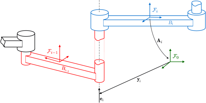
Figure 4: Description of the kinematics of joint $i$ with respect to the spatial IFR in the zero-reference configuration with $\mathbf{q}=\mathbf{0}$.

2.5 Example

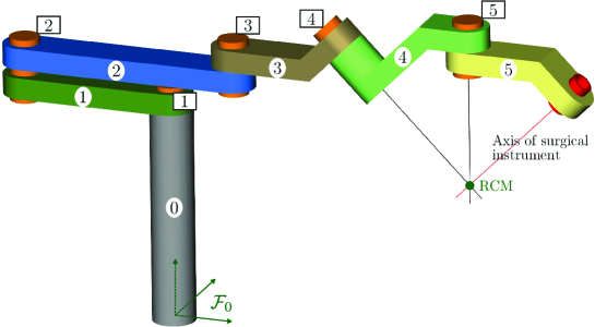
Figure 5: Model of the RCM mechanism disclosed in WonChoiPeine2009 . The model was create with the MBS tool Alaska.

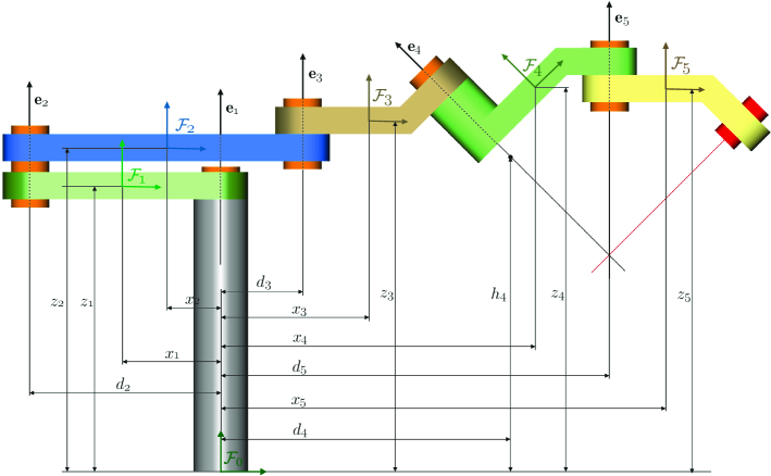
Figure 6: Description of the geometry of the RCM mechanism.

Figure 5 shows a surgical device that consists of a robot arm and a remote center of motion (RCM) mechanism. This was disclosed in the patent WonChoiPeine2009 . The robot arm consisting of bodies 1,2,3 is used to position the RCM mechanism consisting of the bodies 4 and 5. The surgical instrument is mounted in the socket at the remote end of body 5. The axes of joints 4 and 5 and of the instrument intersect at one point. This allows the instrument to freely pivot around an incision point.

The reference configuration is shown in fig. 5. The IFR is located at the base of the mechanism. The joint screw coordinates in spatial representation are determined by the geometric parameters shown in figure 6. The position vectors $\mathbf{y}_{i}$ and unit vectors $\mathbf{e}_{i}$ in (12) are

$$\mathbf{y}_{1} = \left(0,0,0\right)^{T},\mathbf{y}_{2}=\left(-d_{2},0,0\right)^{T},\mathbf{y}_{3}=\left(d_{3},0,0\right)^{T},\mathbf{y}_{4}=\left(d_{4},0,h_{4}\right)^{T},\mathbf{y}_{5}=\left(d_{5},0,0\right)^{T}$$

$$\mathbf{e}_{1} = \mathbf{e}_{2}=\mathbf{e}_{3}=\mathbf{e}_{5}=\left(0,0,1\right)^{T},\mathbf{e}_{4}=(-(1/\sqrt{2},0,1/\sqrt{2})^{T}.$$

Since any point on the joint axes can be used, the 3-components in $\mathbf{y}_{i},i=1,2,3,5$ are set to zero. An arbitrary point on the axis of joint 4 is chosen as indicated. The joint screw coordinates (12) are thus

$$\mathbf{Y}_{1} = \left(0,0,1,0,0,0\right)^{T},\mathbf{Y}_{2}=\left(\{0,0,1,0,d_{2},0\right)^{T},\mathbf{Y}_{3}=\left(0,0,1,0,-d_{3},0\right)^{T}$$

$$\mathbf{Y}_{4} = (-1\sqrt{2},0,1/\sqrt{2},0,-d_{4}/\sqrt{2}-h_{4}/\sqrt{2},0)^{T},\mathbf{Y}_{5}=\left(0,0,1,0,-d_{5},0\right)^{T}.$$

The reference configurations (11) of the bodies are determined by

$$\mathbf{R}_{1}\left(\mathbf{0}\right) = \mathbf{R}_{2}\left(\mathbf{0}\right)=\mathbf{R}_{3}\left(\mathbf{0}\right)=\mathbf{R}_{5}\left(\mathbf{0}\right)=\mathbf{I},\ \mathbf{R}_{4}\left(\mathbf{0}\right)=\left(\begin{array}[]{ccc}1/\sqrt{2}&0&-1/\sqrt{2}\\ 0&1&0\\ 1/\sqrt{2}&0&1/\sqrt{2}\end{array}\right)$$

$$\mathbf{r}_{1}\left(\mathbf{0}\right) = \left(-x_{1},0,z_{1}\right)^{T},\mathbf{r}_{2}\left(\mathbf{0}\right)=\left(-x_{2},0,-z_{2}\right)^{T},\mathbf{r}_{3}\left(\mathbf{0}\right)=\left(x_{3},0,z_{3}\right)^{T}$$

$$\mathbf{r}_{4}\left(\mathbf{0}\right) = \left(x_{4},0,z_{4}\right)^{T},\mathbf{r}_{5}\left(\mathbf{0}\right)=\left(x_{5},0,z_{5}\right)^{T}.$$

Therewith the configuration of all bodies are determined by the POE (10). For instance

$$\mathbf{C}_{3}\left(\mathbf{q}\right)=\left(\begin{array}[]{cccc}c_{123}&-s_{123}&0&-{d_{2}c_{1}}+({d_{2}}+{d_{3}})c_{12}+({x_{3}}-{d_{3}})c_{123}\\ s_{123}&c_{123}&0&-{d_{2}}s_{1}+({d_{2}}+{d_{3}})s_{12}+({x_{3}}-{d_{3}})s_{123}\\ 0&0&1&{z_{3}}\\ 0&0&0&1\end{array}\right)$$

with $c_{123}:=\cos({q_{1}}+{q_{2}}+{q_{3}})$ etc. The expressions for $\mathbf{C}_{4}\left(\mathbf{q}\right)$ and $\mathbf{C}_{5}\left(\mathbf{q}\right)$ are rather complicated and are omitted here.

Instead of deducing them from the geometry in figure 6, the body-fixed representation of the joint screw coordinates can be determined with the relation (12). This yields

$${{}^{1}}\mathbf{X}_{1} = \left(0,0,1,0,-x_{1},0\right)^{T},{{}^{2}}\mathbf{X}_{2}=\left(0,0,1,0,d_{2}-x_{2},0\right)^{T},{{}^{3}}\mathbf{X}_{3}=\left(0,0,1,0,-d_{3}+x_{3},0\right)^{T}$$

$${{}^{4}}\mathbf{X}_{4} = (0,0,1,0,-d_{4}/\sqrt{2}-h_{4}/\sqrt{2}+x_{4}/\sqrt{2}+z_{4}/\sqrt{2},0)^{T},{{}^{5}}\mathbf{X}_{5}=\left(0,0,1,0,-d_{5}+x_{5},0\right)^{T}.$$

This example shows the simplicity of the approach.

3 Velocity of a Kinematic Chain

In this section recursive relations are derived for the four forms of twists that are introduced in appendix A.3, namely the body-fixed, spatial, hybrid, and mixed twists Bruyninckx1996 .

3.1 Body-fixed Representation of Rigid Body Twists

3.1.1 Body-fixed Twists

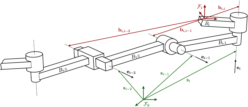
Figure 7: Description of the instantaneous kinematics of a kinematic chain.

The body-fixed twist of body $i$, denoted $\mathbf{V}_{i}^{\text{b}}=(\mathbf{\omega}_{i}^{\text{b}},\mathbf{v}_{i}^{\text{b}})^{T}$, is the aggregate of the angular velocity $\mathbf{\omega}_{i}^{\text{b}}:={{}^{i}}\mathbf{\omega}_{i}$ of its BFR and the translational velocity $\mathbf{v}_{i}^{\text{b}}:={{}^{i}}\mathbf{v}_{i}$ of its origin relative to the IFR (appendix A.2). The twist of body $i$ in a kinematic chain is the sum of twists of the joints connecting it to the ground. Represented (measured and resolved) in its BFR $\mathcal{F}_{i}$ (fig. 7) this is

$$\mathbf{V}_{i}^{\text{b}}=\dot{q}_{1}\left(\begin{array}[]{c}{{}^{i}}\mathbf{e}_{1}\\ {{}^{i}}\mathbf{b}_{i,1}\times{{}^{i}}\mathbf{e}_{1}+{{}^{i}}\mathbf{e}_{1}h_{1}\end{array}\right)+\dot{q}_{2}\left(\begin{array}[]{c}{{}^{i}}\mathbf{e}_{2}\\ {{}^{i}}\mathbf{b}_{i,2}\times{{}^{i}}\mathbf{e}_{2}+{{}^{i}}\mathbf{e}_{2}h_{2}\end{array}\right)+\ldots+\dot{q}_{i}\left(\begin{array}[]{c}{{}^{i}}\mathbf{e}_{i}\\ {{}^{i}}\mathbf{b}_{i,i}\times{{}^{i}}\mathbf{e}_{i}+{{}^{i}}\mathbf{e}_{i}h_{i}\end{array}\right).$$ (14)

Here ${{}^{i}}\mathbf{b}_{i,j}$ is the instantaneous position vector of a point on the axis of joint $j$ measured in the BFR $\mathcal{F}_{i}$, and ${{}^{i}}\mathbf{e}_{j}$ is the unit vector along the axis resolved in the BFR. The instantaneous joint screw coordinates in (14) are configuration dependent, and related to the joint screws (5) and (12) (deduced from reference configuration) by a frame transformation.

3.1.2 Body-Fixed Jacobian and Recursive Relations

The body-fixed twist is determined by (96) in terms of the configuration $\mathbf{C}\left(t\right)$. Using (4) and (93), from $\mathbf{C}_{i}=\mathbf{C}_{i-1}\mathbf{C}_{i-1,i}$ follows the recursive relation (notice $\mathbf{C}_{i-1,i}^{-1}=\mathbf{C}_{i,i-1}=\mathbf{C}_{i}^{-1}\mathbf{C}_{i-1}$)

$$\mathbf{V}_{i}^{\text{b}}=\mathbf{Ad}_{\mathbf{C}_{i,i-1}}\mathbf{V}_{i-1}^{\text{b}}+{{}^{i}}\mathbf{X}_{i}\dot{q}_{i}=\mathbf{Ad}_{\mathbf{B}_{i}\exp({{}^{i}}\mathbf{X}_{i}q_{i})}^{-1}\mathbf{V}_{i-1}^{\text{b}}+{{}^{i}}\mathbf{X}_{i}\dot{q}_{i}.$$ (15)

The frame transformations due to the relative motions $\mathbf{C}_{i,i-1}$ of adjacent bodies propagate the twists within the kinematic chain. The first term on the right hand side of (15) is the twist of body $i-1$ represented in the BFR $\mathcal{F}_{i}$ on body $i$, and the second term is the additional contribution from joint $i$.

The configuration $\mathbf{C}_{i}$ of body $i$ depends on the joint variables $q_{j},j\leq i$. The body-fixed twist (96) can thus be expressed as $\widehat{\mathbf{V}}_{i}^{\text{b}}=\sum_{j\leq i}\widehat{\mathbf{J}}_{i,j}^{\text{b}}\dot{q}_{j}$ where $\widehat{\mathbf{J}}_{i,j}^{\text{b}}:=\mathbf{C}_{i}^{-1}\frac{\partial}{\partial q^{j}}\mathbf{C}_{i}$. The POE (8), together with (93) and (92), yields

$$\mathbf{C}_{i}^{-1}\frac{\partial}{\partial q_{j}}\mathbf{C}_{i} = \exp(-{{}^{i}}\widehat{\mathbf{X}}_{i}q_{i})\mathbf{B}_{i}^{-1}\cdots\exp(-{{}^{j+1}}\widehat{\mathbf{X}}_{j+1}q_{j+1})\mathbf{B}_{j+1}^{-1}{{}^{j}}\widehat{\mathbf{X}}_{j}\exp({{}^{j+1}}\widehat{\mathbf{X}}_{j+1}q_{j+1})\cdots\exp({{}^{i}}\widehat{\mathbf{X}}_{i}q_{i})$$ (16)

$$= \mathbf{C}_{i}^{-1}\mathbf{C}_{j}{{}^{j}}\widehat{\mathbf{X}}_{j}\mathbf{C}_{j}^{-1}\mathbf{C}_{i}=\mathrm{Ad}_{\mathbf{C}_{i,j}}({{}^{j}}\widehat{\mathbf{X}}_{j}),\ j\leq i.$$

Using (12) this yields the following relations

$$\mathbf{J}_{i,j}^{\text{b}}$$

(17)

The $\mathbf{J}_{i,j}^{\text{b}}$ are the screw coordinate vectors in (14) obtained via a frame transformation (89) of ${{}^{j}}\mathbf{X}_{j}$ in (5), or $\mathbf{Y}_{j}$ in (12), to the current configuration. The body-fixed twist is hence

$$\mathbf{V}_{i}^{\text{b}}=\sum_{j\leq i}\mathbf{J}_{i,j}^{\text{b}}\dot{q}_{j}=\mathsf{J}_{i}^{\text{b}}\dot{\mathbf{q}}.$$ (18)

The $6\times n$ matrix

$$\mathsf{J}_{i}^{\text{b}}=\left(\mathbf{J}_{i,1}^{\text{b}},\ldots,\mathbf{J}_{i,i}^{\text{b}},\mathbf{0}\ldots,\mathbf{0}\right)$$ (19)

is called the geometric body-fixed Jacobian of body $i$ Murray . It is the central object in all formulations that use body-fixed twists and Lie group formulations MUBOLieGroup ; ParkBobrowPloen1995 ; Park1994 ; PloenPark1999 . The geometric Jacobian appears in the literature under different names. For instance, in maisser1988 ; maisser1997 ; MUBOLieGroup it is called the ’kinematic basic function (KBF)’ as it is the pivotal object for (recursive) evaluation of MBS kinematics.

The expression (17) gives rise to the recursive relation

$$\mathbf{J}_{i,j}^{\text{b}}=\left\{\begin{array}[]{cl}\mathbf{Ad}_{\mathbf{C}_{i,i-1}}\mathbf{J}_{i-1,j}^{\text{b}},&j<i\vspace{-1ex}\\ &\\ {{}^{i}}\mathbf{X}_{i}&j=i\ \ .\end{array}\right.$$ (20)

This is essentially another form of the recursion (15), using (18).

Remark 5 (Dependence on joint variables)

With (8), respectively (10), it is clear that the Jacobian $\mathbf{J}_{i}^{\text{b}}$ of body $i$ can only depend on $q_{1},\ldots,q_{i}$. Moreover, noting in (17) that $\mathbf{C}_{i,j}=\mathbf{C}_{i}^{-1}\mathbf{C}_{j}$ is independent from $q_{1}$, it follows that $\mathbf{J}_{i}^{\text{b}}$ depends on $q_{2},\ldots,q_{i}$, i.e. it is independent from the first joint in the chain. This is obvious from a kinematic perspective since $\mathbf{V}_{i}^{\text{b}}$ is the sum of twists of the preceding bodies in the chain expressed in the BFR on body $i$. This only depends on the configuration of the bodies relative to body $i$ but not on the absolute configuration of the overall chain, which is determined by $q_{1}$.

Remark 6 (Required data)

The second form in (17) in conjunction with (10) allows for computation of the body-fixed Jacobian without introducing body-fixed JFRs. The only information needed are the joint screw coordinates $\mathbf{Y}_{j}$ represented in the IFR and the reference configurations $\mathbf{A}_{j}$.

Remark 7 (Change of reference frame)

When another BFR on body $i$ is used, which is related to the original BFR by $\mathbf{S}\in SE\left(3\right)$, its configuration is given by $\mathbf{C}_{i}^{\prime}=\mathbf{C}_{i}\mathbf{S}$. The corresponding body-fixed twist follows from (96) as $\widehat{\mathbf{V}}_{i}^{\prime\text{b}}=\mathbf{C}_{i}^{\prime-1}\dot{\mathbf{C}}_{i}^{\prime}=\mathbf{S}^{-1}\mathbf{C}_{i}^{-1}\dot{\mathbf{C}}_{i}\mathbf{S}=\mathrm{Ad}_{\mathbf{S}}^{-1}(\widehat{\mathbf{V}}_{i}^{\text{b}})$, and in vector form

$$\mathbf{V}_{i}^{\prime\text{b}}=\mathbf{Ad}_{\mathbf{S}}^{-1}\mathbf{V}_{i}^{\text{b}}.$$ (21)

On the other hand the body-fixed twist is invariant under a change of IFR, which is given by $\mathbf{C}_{i}^{\prime}=\mathbf{SC}_{i}$. Body-fixed twists are therefore called left-invariant vector fields on $SE\left(3\right)$ since left multiplication of $\mathbf{C}_{i}$ with any $\mathbf{S}\in SE\left(3\right)$ does not affect $\mathbf{V}_{i}^{\text{b}}$.

Remark 8 (Application of body-fixed representation)

The recursive relations for body-fixed twist and Jacobian are the basis for the MBS dynamics algorithms in Anderson1992 ; AndersonCritchley2003 ; Bae2001 ; Fijany1995 ; Hollerbach1980 ; LillyOrin1991 ; Liu1988 ; ParkBobrowPloen1995 ; Park1994 ; PloenPark1999 ; VukobratovicPotkonjak1979 . In Anderson1992 ; AndersonCritchley2003 the adjoint transformation matrix in (15) was called the ’shift matrix’, and $\mathbf{X}_{i}$ was called the ’motion map matrix’. However, the geometric background was rarely exploited as in ParkBobrowPloen1995 ; Park1994 ; PloenPark1999 and Liu1988 . Remarkably Liu Liu1988 already presented all relevant formulations in terms of screws.

3.1.3 Body-Fixed System Jacobian and its Decomposition

The body-fixed twists are summarized in the overall twist vector $\mathsf{V}^{\text{b}}=(\mathbf{V}_{1}^{\text{b}},\ldots,\mathbf{V}_{n}^{\text{b}})^{T}$. The recursion (15) can then be written in matrix form

$$\mathsf{V}^{\text{b}}=\mathsf{D}^{\text{b}}\mathsf{V}^{\text{b}}+\mathsf{X}^{\text{b}}\dot{\mathbf{q}}$$ (22)

with

$$\mathsf{D}^{\text{b}}:=\left(\begin{array}[]{ccccc}\mathbf{0}&\mathbf{0}&\mathbf{0}&&\mathbf{0}\\ \mathbf{Ad}_{\mathbf{C}_{2,1}}&\mathbf{0}&\mathbf{0}&\cdots&\\ \mathbf{0}&\mathbf{Ad}_{\mathbf{C}_{3.2}}&\mathbf{0}&&\\ \vdots&\vdots&\ddots&\ddots&\\ \mathbf{0}&\mathbf{0}&\cdots&\mathbf{Ad}_{\mathbf{C}_{n,n-1}}&\mathbf{0}\end{array}\right),\ \mathsf{X}^{\text{b}}:=\mathrm{diag}~{}\left({{}^{1}\mathbf{X}}_{1},\ldots,{{}^{n}}\mathbf{X}_{n}\right).$$ (23)

On the other hand, the recursive expression for the Jacobian (20) reads in matrix form

$$\mathsf{V}^{\text{b}}=\mathsf{J}^{\text{b}}\dot{\mathbf{q}}=\mathsf{A}^{\text{b}}\mathsf{X}^{\text{b}}\dot{\mathbf{q}}$$ (24)

where the $6n\times n$ matrix $\mathsf{J}^{\text{b}}=\mathsf{A}^{\text{b}}\mathsf{X}^{\text{b}}$ is the system Jacobian in body-fixed representation, and

$$\mathsf{A}^{\text{b}}:=\left(\begin{array}[]{ccccc}\mathbf{I}&\mathbf{0}&\mathbf{0}&&\mathbf{0}\\ \mathbf{Ad}_{\mathbf{C}_{2,1}}&\mathbf{I}&\mathbf{0}&\cdots&\mathbf{0}\\ \mathbf{Ad}_{\mathbf{C}_{3,1}}&\mathbf{Ad}_{\mathbf{C}_{3,2}}&\mathbf{I}&&\mathbf{0}\\ \vdots&\vdots&\ddots&\ddots&\\ \mathbf{Ad}_{\mathbf{C}_{n,1}}&\mathbf{Ad}_{\mathbf{C}_{n,2}}&\cdots&\mathbf{Ad}_{\mathbf{C}_{n,n-1}}&\mathbf{I}\end{array}\right)$$ (25)

is the screw transformation matrix. Comparing (22) and (24) shows that $\mathsf{A}^{\text{b}}=(\mathbf{I}-\mathsf{D}^{\text{b}})^{-1}$. In fact $\mathsf{D}^{\text{b}}$ is nilpotent so that the von-Neumann series

$$\mathsf{A}^{\text{b}}=(\mathbf{I}-\mathsf{D}^{\text{b}})^{-1}=\mathbf{I}+\mathsf{D}^{\text{b}}+(\mathsf{D}^{\text{b}})^{2}+\ldots+(\mathsf{D}^{\text{b}})^{n}$$ (26)

terminates with $(\mathsf{D}^{\text{b}})^{n+1}=0$. That is, $\mathbf{A}^{\text{b}}$ is the 1-resolvent of $\mathsf{D}^{\text{b}}$, which is the fundamental point of departure for many $O\left(n\right)$ algorithms. Moreover, (26) is another form of the recursive coordinate transformations. Hence the inverse $(\mathsf{A}^{\text{b}})^{-1}=(\mathbf{I}-\mathsf{D}^{\text{b}})$.

Remark 9 (Overall inverse kinematics solution)

The above result allows for a simple transformation from body-fixed velocities to the corresponding joint rates. When the twists of all bodies are given, (24) is an overdetermined linear system in $\dot{\mathbf{q}}$. It has a unique solution as long as the twists are consistent with the kinematics. Premultiplication of (24) with $(\mathbf{I}-\mathsf{D}^{\text{b}})$ followed by $(\mathsf{X}^{\text{b}})^{T}$ and $((\mathsf{X}^{\text{b}})^{T}\mathsf{X}^{\text{b}})^{-1}$ yields

$$\dot{\mathbf{q}}=((\mathsf{X}^{\text{b}})^{T}\mathsf{X}^{\text{b}})^{-1}(\mathsf{X}^{\text{b}})^{T}(\mathbf{I}-\mathsf{D}^{\text{b}})\mathsf{V}^{\text{b}}.$$ (27)

The $n\times n$ diagonal matrix $(\mathsf{X}^{\text{b}T}\mathsf{X}^{\text{b}})^{-1}=\mathrm{diag}(1/\left\|{{}^{1}\mathbf{X}}_{1}\right\|^{2},\ldots,1/\left\|{{}^{n}\mathbf{X}}_{n}\right\|^{2})$ has full rank. Due to the block diagonal structure this yields the solutions $\dot{q}_{i}={{}^{i}\mathbf{X}}_{i}^{T}(\mathbf{V}_{i}^{\text{b}}-\mathbf{Ad}_{\mathbf{C}_{i,i-1}}\mathbf{V}_{i-1}^{\text{b}})/\left\|{{}^{i}\mathbf{X}}_{i}\right\|^{2}$ for the individual joints. This is indeed the projection of the relative twist of body $i$ w.r.t. body $i-1$ onto the axis of joint $i$. It is an exact solution of the inverse kinematics for the overall MBS, presumed that the twists are compatible, i.e. satisfy (15). If this is not the case, (27) is the unique pseudoinverse solution of the system (24) of $6n$ equations for the $n$ unknown $\dot{q}_{i}$ minimizing the residual error. This can be considered as the generalized inverse kinematics problem: given desired twists of all individual links, find the joint rates that best reproduce these twists. This can be applied, for instance, to the inverse kinematics of human body models processing motion capture data (estimated position and orientation of body segments) and when noisy data is processed.

While the solution (27) seems straightforward, it should be remarked that there is no frame invariant inner product on $se\left(3\right)$, i.e. no norm of screws can be defined that is invariant under a change of reference frame Selig . The correctness of (27) follows by regarding the transposed joint screw coordinates as co-screws, and ${{}^{i}\mathbf{X}}_{i}^{T}{{}^{i}\mathbf{X}}_{i}$ is the pairing of screw and co-screw coordinates rather than an inner product.

3.2 Spatial Representation of Rigid Body Twists

3.2.1 Spatial Twists

A representation of the body twist, which is less common in MBS modeling but frequently used in mechanism theory, is the so-called spatial twist denoted $\mathbf{V}_{i}^{\text{s}}=(\mathbf{\omega}_{i}^{\text{s}},\mathbf{v}_{i}^{\text{s}})^{T}$. This is the twist of body $i$ represented in the IFR. It consists of the angular velocity of the BFR of body $i$ measured and resolved in the IFR, and the translational velocity $\mathbf{v}_{i}^{\text{s}}:=\dot{\mathbf{r}}_{i}-\mathbf{\omega}_{i}^{\text{s}}\times\mathbf{r}_{i}$ of the (possibly imaginary) point on the body that is momentarily traveling through the origin of the IFR measured and resolved in the IFR (appendix A.2). With the notation in fig. 7, the spatial twist of body $i$ is geometrically readily constructed as

$$\mathbf{V}_{i}^{\text{s}}=\dot{q}_{1}\left(\begin{array}[]{c}\mathbf{e}_{1}\\ \mathbf{s}_{1}\times\mathbf{e}_{1}+h_{1}\mathbf{e}_{1}\end{array}\right)+\dot{q}_{2}\left(\begin{array}[]{c}\mathbf{e}_{2}\\ \mathbf{s}_{2}\times\mathbf{e}_{2}+h_{2}\mathbf{e}_{2}\end{array}\right)+\ldots+\dot{q}_{i}\left(\begin{array}[]{c}\mathbf{e}_{i}\\ \mathbf{s}_{i}\times\mathbf{e}_{i}+h_{i}\mathbf{e}_{i}\end{array}\right)$$ (28)

where $\mathbf{s}_{j}$ is the position vector of a point on the joint axis $j$ expressed in the IFR. The screw coordinates in (28) are configuration dependent. They are equal to $\mathbf{Y}_{j}$ in the reference configuration $\mathbf{q}=\mathbf{0}$, where $\mathbf{s}_{i}=\mathbf{y}_{i}$.

3.2.2 Spatial Jacobian and Recursive Relations

In order to derive an analytic expression, using the POE, the definition (96) of the spatial twist is applied. As apparent from (28), the non-vanishing instantaneous joint screws are identical for all bodies. This is clear since the IFR is the only reference frame involved. The spatial twist can thus be expressed as $\mathbf{V}_{i}^{\text{s}}=\sum_{j\leq i}\mathbf{J}_{j}^{\text{s}}\dot{q}_{j}$ with $\widehat{\mathbf{J}}_{j}^{\text{s}}:=\frac{\partial}{\partial q_{j}}\mathbf{C}_{i}\mathbf{C}_{i}^{-1}$. Using the POE, a straightforward derivation analogous to (16) yields

$$\mathbf{J}_{j}^{\text{s}}$$

(29)

The $\mathbf{J}_{j}^{\text{s}}$ is the instantaneous screw coordinate vector of joint $j$ in (28) in spatial representation, i.e. represented in the IFR. The matrix

$$\mathsf{J}_{i}^{\text{s}}=\Big{(}\mathbf{J}_{1}^{\text{s}},\ldots,\mathbf{J}_{i}^{\text{s}},\mathbf{0},\ldots,\mathbf{0}\Big{)}$$ (30)

is called the spatial Jacobian of body $i$. The relations (28) and (29) yield the following recursive expression for the spatial twists of bodies in a kinematic chain

$$\mathbf{V}_{i}^{\text{s}}=\mathbf{V}_{i-1}^{\text{s}}+\mathbf{J}{{}_{i}^{\text{s}}}\dot{q}_{i}.$$ (31)

Remark 10

The spatial representation has remarkable advantages. The velocity recursion (31) is the simplest possible since the twists of individual bodies can simply be added without any coordinate transformation. An important observation is that $\mathbf{J}_{j}^{\text{s}}$ is intrinsic to the joint $j$. The non-zero screw vectors in the Jacobian (30) are thus the same for all bodies. This is a consequence of using a single spatial reference frame.

3.2.3 Spatial System Jacobian and its Decomposition

The overall spatial twist $\mathsf{V}^{\text{s}}=(\mathbf{V}_{1}^{\text{s}},\ldots,\mathbf{V}_{n}^{\text{s}})^{T}$ of the kinematic chain is determined as

$$\mathsf{V}^{\text{s}}=\mathsf{J}^{\text{s}}\dot{\mathbf{q}}$$ (32)

where the spatial system Jacobian possesses the factorizations

$$\mathsf{J}^{\text{s}}=\mathsf{A}^{\text{s}}\mathsf{Y}^{\text{s}}=\mathsf{A}^{\text{sb}}\mathsf{X}^{\text{b}}=\mathsf{A}^{\text{sh}}\mathsf{X}^{\text{h}}.$$ (33)

Therein it is $\mathsf{Y}^{\text{s}}=\mathrm{diag}~{}\left({\mathbf{Y}}_{1},\ldots,\mathbf{Y}_{n}\right)$, $\mathsf{X}^{\text{h}}$ in (60), and

$$\mathsf{A}^{\text{sb}}:= \left(\begin{array}[]{ccccc}\mathbf{Ad}_{\mathbf{C}_{1}}&\mathbf{0}&\mathbf{0}&&\mathbf{0}\\ \mathbf{Ad}_{\mathbf{C}_{1}}&\mathbf{Ad}_{\mathbf{C}_{2}}&\mathbf{0}&&\mathbf{0}\\ \mathbf{Ad}_{\mathbf{C}_{1}}&\mathbf{Ad}_{\mathbf{C}_{2}}&\mathbf{Ad}_{\mathbf{C}_{3}}&&\mathbf{0}\\ \vdots&\vdots&\ddots&\ddots&\vdots\\ \mathbf{Ad}_{\mathbf{C}_{1}}&\mathbf{Ad}_{\mathbf{C}_{2}}&\cdots&\mathbf{Ad}_{\mathbf{C}_{n-1}}&\mathbf{Ad}_{\mathbf{C}_{n}}\end{array}\right),\ \ \ \mathsf{A}^{\text{sh}}:=\left(\begin{array}[]{ccccc}\mathbf{Ad}_{\mathbf{r}_{1}}&\mathbf{0}&\mathbf{0}&&\mathbf{0}\\ \mathbf{Ad}_{\mathbf{r}_{1}}&\mathbf{Ad}_{\mathbf{r}_{2}}&\mathbf{0}&&\mathbf{0}\\ \mathbf{Ad}_{\mathbf{r}_{1}}&\mathbf{Ad}_{\mathbf{r}_{2}}&\mathbf{0}&&\mathbf{0}\\ \vdots&\vdots&\ddots&\ddots&\\ \mathbf{Ad}_{\mathbf{r}_{1}}&\mathbf{Ad}_{\mathbf{r}_{2}}&\cdots&\mathbf{Ad}_{\mathbf{r}_{n-1}}&\mathbf{Ad}_{\mathbf{r}_{n}}\end{array}\right)\ \ \ \$$ (44)

$$\mathsf{A}^{\text{s}}:= \mathsf{A}^{\text{sb}}\mathrm{diag}~{}(\mathbf{Ad}_{\mathbf{A}_{1}}^{-1},\ldots,\mathbf{Ad}_{\mathbf{A}_{n}}^{-1}).$$

All non-zero entries in a column of these matrices are identical. Hence the construction of these matrices only requires determination of the $n$ entries in the last row that are copied into the upper triangular block matrix. The factorization (33) gives rise to an expression for its inverse. Noting $\mathsf{A}^{\text{sb}}=\mathrm{diag}~{}(\mathbf{Ad}_{\mathbf{C}_{1}},\ldots,\mathbf{Ad}_{\mathbf{C}_{n}})\mathsf{A}^{\text{b}}$ the relation for the inverse of $\mathsf{A}^{\text{b}}$ in terms of matrix $\mathsf{D}^{\text{b}}$ in (23) yields

$$(\mathsf{A}^{\text{sb}})^{-1} = (\mathbf{I}-\mathsf{D}^{\text{b}})\mathrm{diag}~{}(\mathbf{Ad}_{\mathbf{C}_{1}},\ldots,\mathbf{Ad}_{\mathbf{C}_{n}})$$ (50)

$$= \left(\begin{array}[]{ccccc}\mathbf{Ad}_{\mathbf{C}_{1}}^{-1}&\mathbf{0}&\mathbf{0}&&\mathbf{0}\\ -\mathbf{Ad}_{\mathbf{C}_{2}}&\mathbf{Ad}_{\mathbf{C}_{2}}^{-1}&\mathbf{0}&&\mathbf{0}\\ \mathbf{0}&-\mathbf{Ad}_{\mathbf{C}_{3}}&\mathbf{Ad}_{\mathbf{C}_{3}}^{-1}&&\mathbf{0}\\ \vdots&\vdots&\ddots&\ddots&\vdots\\ \mathbf{0}&\mathbf{0}&\cdots&-\mathbf{Ad}_{\mathbf{C}_{n}}&\mathbf{Ad}_{\mathbf{C}_{n}}^{-1}\end{array}\right)$$

and $(\mathsf{A}^{\text{s}})^{-1}$ accordingly.

Remark 11 (Dependence on joint variables)

Similarly to the body-fixed twist, it follows from $\mathbf{J}_{i}^{\text{s}}=\mathbf{Ad}_{\mathbf{C}_{i}}{{}^{i}}\mathbf{X}_{i}=\mathbf{Ad}_{\mathbf{C}_{i-1}}\mathbf{Ad}_{\mathbf{B}_{i}\exp{{}^{i}}\mathbf{X}_{i}q_{i}}{{}^{i}}\mathbf{X}_{i}=\mathbf{Ad}_{\mathbf{C}_{i-1}}{{}^{i}}\mathbf{X}_{i}$ being independent from $q_{i}$, that the spatial Jacobian of body $i$ only depends on $q_{1},\ldots,q_{i-1}$. Indeed, the motion of joint $i$ does not change its screw axis about which body $i$ is moving.

Remark 12 (Change of reference frame)

The spatial twist is called a right-invariant vector field on $SE\left(3\right)$ because it does not change when $\mathbf{C}_{i}$ is postmultiplied by any $\mathbf{S}\in SE\left(3\right)$, representing a change of body-fixed RFR. Under a change of IFR according to $\mathbf{C}_{i}^{\prime}=\mathbf{SC}_{i}$ the spatial twists transform as

$$\mathbf{V}_{i}^{\prime\text{s}}=\mathbf{Ad}_{\mathbf{S}}\mathbf{V}_{i}^{\text{s}}.$$ (51)

Remark 13 (Application of spatial representation)

The spatial twist is used almost exclusively in mechanism kinematics (often without mentioning it) but is becoming accepted for MBS modeling since it was introduced in Featherstone1983 ; Featherstone2008 . For kinematic analysis of mechanisms it is common practice to (instantaneously) locate the global reference frame so that it coincides with the frame where kinetostatic properties (twists, wrenches) are observed, usually at the end-effector. For a serial robotic manipulator the end-effector frame is located at the terminal link of the chain, so that $\mathbf{A}_{n}=\mathbf{I}$, and $\mathbf{V}_{n}^{\text{s}}$ is then the spatial end-effector twist. From their definition follows that the spatial and hybrid twist (see next section) of body $i$ are numerically identical when the BFR $\mathcal{F}_{i}$ overlaps with the IFR $\mathcal{F}_{0}$.
The most prominent use of the spatial representation in dynamics is the $O\left(n\right)$ forward dynamics method by Featherstone Featherstone1983 ; Featherstone2008 . This has not yet been widely applied in MBS dynamics. This may be due to use of an uncommon choice of reference point (the IFR origin) at which the spatial entities are measured, so that results and interaction wrenches must be transformed to body-fixed reference frames. The spatial representation of twists must not be confused with the ’spatial vector’ notation proposed in Featherstone1983 ; Featherstone2008 . The latter is a general expression of twists as 6-vectors (like body-fixed and spatial) but without reference to a particular frame in which the components are resolved. This allows for abstract derivation of kinematic relations, but these relation must eventually be resolved in a particular frame, and this eventually determines the computational effort.
A notable application of the spatial twist is the modeling and numerical integration of non-linear elastic MBS where it is called the base pole velocity Borri2001a or fixed pole velocity Bottasso1998 and the intrinsic coupling of translational and angular velocity (according to the screw motion) was discussed. The corresponding momentum balance and conservation properties are discussed in Borri2001b ; Borri2003 (see also Part2 ).

Remark 14

As in remark 9, the relation (50) gives rise to an overall inverse kinematics solution. For given spatial twists $\mathbf{V}_{i}^{\text{s}}$ this reads in components $\dot{q}_{i}={{}^{i}\mathbf{X}}_{i}^{T}\mathbf{Ad}_{\mathbf{C}_{i}}^{-1}(\mathbf{V}_{i}^{\text{s}}-\mathbf{V}_{i-1}^{\text{s}})/\left\|{{}^{i}\mathbf{X}}_{i}\right\|^{2}$.

3.3 Hybrid Form of Rigid Body Twists

3.3.1 Hybrid Twists

In various applications it is beneficial to measure the twist of a body in the body-fixed BFR but resolve it in the IFR. This is commonly referred to as the hybrid twist Bruyninckx1996 ; Murray , denoted $\mathbf{V}_{i}^{\text{h}}=(\mathbf{\omega}_{i}^{\text{s}},\dot{\mathbf{r}}_{i})^{T}$. The geometric construction (fig. 7) yields

$$\mathbf{V}_{i}^{\text{h}}=\dot{q}_{1}\left(\begin{array}[]{c}\mathbf{e}_{1}\\ \mathbf{b}_{i,1}\times\mathbf{e}_{1}+h_{1}\mathbf{e}_{1}\end{array}\right)+\dot{q}_{2}\left(\begin{array}[]{c}\mathbf{e}_{2}\\ \mathbf{b}_{i,2}\times\mathbf{e}_{2}+h_{2}\mathbf{e}_{2}\end{array}\right)+\ldots+\dot{q}_{i}\left(\begin{array}[]{c}\mathbf{e}_{i}\\ \mathbf{b}_{i,i}\times\mathbf{e}_{i}+h_{i}\mathbf{e}_{i}\end{array}\right).$$ (52)

As in (14), $\mathbf{b}_{i,j}$ is the position vector of a point on the axis of joint $j$ measured from the BFR $\mathcal{F}_{i}$ of body $i$, and $\mathbf{e}_{j}$ is a unit vector along the axis, but now expressed in the IFR $\mathcal{F}_{0}$. This was originally introduced in Waldron1982 and Whitney1972 and is used in various $O\left(n\right)$ dynamics algorithms (remark 15).

3.3.2 Hybrid Jacobian and Recursive Relations

The hybrid twist is merely the body-fixed twist resolved in the IFR. Using (91) this transformation is $\mathbf{V}_{i}^{\text{h}}=\mathbf{Ad}_{\mathbf{R}_{i}}\mathbf{V}_{i}^{\text{b}}$ where $\mathbf{R}_{i}$ is the rotation matrix of body $i$. Then (18) leads to

$$\mathbf{V}_{i}^{\text{h}}=\sum_{j\leq i}\mathbf{J}_{i,j}^{\text{h}}\dot{q}_{j}=\mathsf{J}_{i}^{\text{h}}\dot{\mathbf{q}}$$ (53)

with the columns $\mathbf{J}_{i,j}^{\text{h}}:=\mathbf{Ad}_{\mathbf{R}_{i}}\mathbf{J}_{i,j}^{\text{b}}$ of the hybrid Jacobian $\mathsf{J}_{i}^{\text{h}}=\left(\mathbf{J}_{i,1}^{\text{h}},\ldots,\mathbf{J}_{i,i}^{\text{h}},\mathbf{0}\ldots,\mathbf{0}\right)$. The recursive expressions (20) and (15) remain valid when all screw coordinate vectors are resolved in the IFR. The joint screw coordinates are then configuration dependent. The screw coordinate vector of joint $j$ measured in the BFR $\mathcal{F}_{j}$ on body $j$ and resolved in the IFR $\mathcal{F}_{0}$ is related to (5) via

$${{}^{0}}\mathbf{X}_{j}^{j}=\mathbf{Ad}_{\mathbf{R}_{j}}{{}^{j}}\mathbf{X}_{j}=\left(\begin{array}[]{c}\mathbf{e}_{j}\\ \mathbf{x}_{j,j}\times\mathbf{e}_{j}+h_{j}\mathbf{e}_{j}\end{array}\right).$$ (54)

As in (5), the position vector $\mathbf{x}_{j,j}$ of a point on the axis of joint $j$ measured from the BFR $\mathcal{F}_{j}$ but now resolved in the IFR. The relations $\mathbf{Ad}_{\mathbf{C}_{i}}=\mathbf{Ad}_{\mathbf{r}_{i}}\mathbf{Ad}_{\mathbf{R}_{i}}$ and $\mathbf{r}_{i,j}=\mathbf{r}_{j}-\mathbf{r}_{i}$ lead to

$$\mathbf{Ad}_{\mathbf{R}_{i}}\mathbf{J}_{i,j}^{\text{b}} = \mathbf{Ad}_{\mathbf{R}_{i}}\mathbf{Ad}_{\mathbf{C}_{i,j}}{{}^{j}}\mathbf{X}_{j}=\mathbf{Ad}_{\mathbf{R}_{i}}\mathbf{Ad}_{\mathbf{C}_{i,j}}\mathbf{Ad}_{\mathbf{R}_{j}}^{-1}{{}^{0}}\mathbf{X}_{j}^{j}=\mathbf{Ad}_{\mathbf{R}_{i}}\mathbf{Ad}_{\mathbf{C}_{i}}^{-1}\mathbf{Ad}_{\mathbf{C}_{j}}\mathbf{Ad}_{\mathbf{R}_{j}}^{-1}{{}^{0}}\mathbf{X}_{j}^{j}$$ (55)

$$= \mathbf{Ad}_{\mathbf{r}_{i}}^{-1}\mathbf{Ad}_{\mathbf{r}_{j}}{{}^{0}}\mathbf{X}_{j}^{j}=\mathbf{Ad}_{-\mathbf{r}_{i}}\mathbf{Ad}_{\mathbf{r}_{j}}{{}^{0}}\mathbf{X}_{j}^{j}=\mathbf{Ad}_{\mathbf{r}_{j}-\mathbf{r}_{i}}{{}^{0}}\mathbf{X}_{j}^{j}=\mathbf{Ad}_{\mathbf{r}_{i,j}}{{}^{0}}\mathbf{X}_{j}^{j}.$$

Therewith the columns of the hybrid Jacobian of body $i$ are

$$\mathbf{J}_{i,j}^{\text{h}}=\mathbf{Ad}_{\mathbf{r}_{i,j}}{{}^{0}}\mathbf{X}_{j}^{j},\ \ j\leq i.$$

(56)

The $\mathbf{J}_{i,j}^{\text{h}}$ is the instantaneous screw coordinate of joint $j$ in (52) measured at BFR on body $i$ and resolved in the IFR. In the hybrid form, all vectors are resolved in the IFR. That is, the screw coordinates ${{}^{0}}\mathbf{X}_{j}^{j}$ depend on the current configuration $\mathbf{q}$ even though the joint axis is constant within body $j$. The hybrid twist is resolved in the IFR. Since the screw coordinates ${{}^{0}}\mathbf{X}_{j}^{j}$ are already resolved in the IFR the transformation to the current configuration, in order to determine the instantaneous joint screws $\mathbf{J}_{i,j}^{\text{h}}\left(\mathbf{q}\right)$, only requires translations of origins. This is obtained by shifting the reference point according to $\mathbf{r}_{i,j}$, which is why the matrix $\mathbf{Ad}_{\mathbf{r}_{i,j}}$ is also called the ’shift dyad’ CritchleyAnderson2003 . This is not a frame transformation.

The relation (56) gives rise to the recursive relation for the hybrid Jacobian

$$\mathbf{J}_{i,j}^{\text{h}}=\left\{\begin{array}[]{cl}\mathbf{Ad}_{\mathbf{r}_{i,i-1}}\mathbf{J}_{i-1,j}^{\text{h}},&j<i\vspace{-1ex}\\ &\\ {{}^{0}}\mathbf{X}_{i}^{i},&j=i\ .\end{array}\right.\ \$$ (57)

and, analogous to (15), for the hybrid twists

$$\mathbf{V}_{i}^{\text{h}}=\mathbf{Ad}_{\mathbf{r}_{i,i-1}}\mathbf{V}_{i-1}^{\text{h}}+{{}^{0}}\mathbf{X}_{i}^{i}\dot{q}^{i}.$$ (58)

The advantage of the hybrid form over the body-fixed is that (57) only involves the relative displacement $\mathbf{r}_{i,i-1}$ in contrast to the complete relative configuration $\mathbf{C}_{i,i-1}$ in (20). It must be recalled, however, that the vectors $\mathbf{e}_{j}$ and $\mathbf{r}_{j,j}$ must be transformed to the IFR. Furthermore, when formulating equations of motion, the inertia properties of the body must be resolved in the IFR so that they become configuration dependent Part2 .

Remark 15 (Application of hybrid representation)

The hybrid form was used in Waldron1982 for forward kinematics calculation of serial manipulators, and in AngelesLee1988 ; Angeles2003 to compute the motion equations respectively the inverse dynamics solution. It is used in many recursive $O\left(n\right)$ forward dynamics algorithms such as BaeHwangHaug1988 ; LillyOrin1991 ; Naudet2003 ; Orin1979 ; Rodriguez1991 where the relations (58) and (56) play a central role. In the so-called ’spatial operator algebra’ Rodriguez1991 , hybrid screw entities are called ’spatial vectors’. The hybrid form is deemed computationally efficient since the transformations only involve translations. The actual configuration of the chain is not discussed in these publications, but it enters via the vectors $\mathbf{e}_{i}\left(\mathbf{q}\right)$ and $\mathbf{r}_{i}\left(\mathbf{q}\right)$, respectively $\mathbf{d}_{i,j}\left(\mathbf{q}\right)$. In LillyOrin1991 the inverse transformation $\mathbf{Ad}_{\mathbf{r}_{i,j}}^{-1}$ was denoted with ${}^{j}\mathbf{X}_{i}$ (not to be confused with (5)), and the screw coordinate vector ${{}^{0}}\mathbf{X}_{j}^{j}$ in (54) with $\phi_{j}$. In Rodriguez1991 , $\mathbf{Ad}_{\mathbf{r}_{i,j}}^{-1}$ was denoted with $\phi_{i,j}^{T}$, and ${{}^{0}}\mathbf{X}_{j}^{j}$ with $\mathbf{H}_{j}^{T}$. The transposed matrices appear since they arose from the transformation of wrenches.

3.3.3 Hybrid System Jacobian and its Decomposition

The hybrid system Jacobian, which determines the overall hybrid twist vector $\mathsf{V}^{\text{h}}=(\mathbf{V}_{1}^{\text{h}},\ldots,\mathbf{V}_{n}^{\text{h}})^{T}$ according to

$$\mathsf{V}^{\text{h}}=\mathsf{J}^{\text{h}}\dot{\mathbf{q}}=\mathsf{A}^{\text{h}}\mathsf{X}^{\text{h}}\dot{\mathbf{q}},$$ (59)

is decomposed in terms of

$$\mathsf{A}^{\text{h}}:=\left(\begin{array}[]{ccccc}\mathbf{I}&\mathbf{0}&\mathbf{0}&&\mathbf{0}\\ \mathbf{Ad}_{\mathbf{r}_{2,1}}&\mathbf{I}&\mathbf{0}&&\mathbf{0}\\ \mathbf{Ad}_{\mathbf{r}_{3,1}}&\mathbf{Ad}_{\mathbf{r}_{3,2}}&\mathbf{I}&&\mathbf{0}\\ \vdots&\vdots&\ddots&\ddots&\\ \mathbf{Ad}_{\mathbf{r}_{n,1}}&\mathbf{Ad}_{\mathbf{r}_{n,2}}&\cdots&\mathbf{Ad}_{\mathbf{r}_{n,n-1}}&\mathbf{I}\end{array}\right),~{}~{}~{}\mathsf{X}^{\text{h}}:=\mathrm{diag}~{}\left({{}^{0}}\mathbf{X}_{1}^{1},\ldots,{{}^{0}}\mathbf{X}_{n}^{n}\right).$$ (60)

In analogy to (26), $\mathsf{A}^{\text{h}}$ can be resolved as power series using the relation $\mathsf{A}^{\text{h}}=(\mathbf{I}-\mathsf{T}^{\text{h}})^{-1}$ with the $6n\times 6n$ matrix

$$\mathsf{T}^{\text{h}}:=\left(\begin{array}[]{ccccc}\mathbf{0}&\mathbf{0}&\mathbf{0}&&\mathbf{0}\\ \mathbf{Ad}_{\mathbf{r}_{2,1}}&\mathbf{0}&\mathbf{0}&&\\ \mathbf{0}&\mathbf{Ad}_{\mathbf{r}_{3,2}}&\mathbf{0}&&\\ \vdots&\vdots&\ddots&\ddots&\\ \mathbf{0}&\mathbf{0}&\cdots&\mathbf{Ad}_{\mathbf{r}_{n,n-1}}&\mathbf{0}\end{array}\right).$$ (61)

This leads to the inverse $(\mathsf{A}^{\text{h}})^{-1}=(\mathbf{I}-\mathsf{T}^{\text{h}})$, and a solution $\dot{\mathbf{q}}$ of (59) of the form (27).

3.4 Mixed Form of Rigid Body Twists

3.4.1 Mixed Twists

When formulating the Newton-Euler equations of rigid bodies, it can be beneficial to use the body-fixed angular velocity and the translational velocity measured at the body-fixed BFR but resolved in the IFR. This is called the mixed twist denoted with $\mathbf{V}_{i}^{\text{m}}=(\mathbf{\omega}_{i}^{\text{b}},\dot{\mathbf{r}}_{i})^{T}$. It is used in MBS dynamics modeling Shabana , basically because when using the mixed twist the Newton-Euler equations w.r.t. the COM are decoupled, and because the body-fixed inertia tensor is constant (see also the companion paper Part2 ). The mixed twist is readily found as

$$\mathbf{V}_{i}^{\text{m}}=\dot{q}_{1}\left(\begin{array}[]{c}{{}^{i}}\mathbf{e}_{1}\\ \mathbf{b}_{i,1}\times\mathbf{e}_{1}+\mathbf{e}_{1}h_{1}\end{array}\right)+\dot{q}_{2}\left(\begin{array}[]{c}{{}^{i}}\mathbf{e}_{2}\\ \mathbf{b}_{i,2}\times\mathbf{e}_{2}+\mathbf{e}_{2}h_{2}\end{array}\right)+\ldots+\dot{q}_{i}\left(\begin{array}[]{c}{{}^{i}}\mathbf{e}_{i}\\ \mathbf{b}_{i,i}\times\mathbf{e}_{i}+\mathbf{e}_{i}h_{i}\end{array}\right).$$ (62)

As in (52), $\mathbf{e}_{j}$ is a unit vector along the axis of joint $j$ measured and resolved in the IFR $\mathcal{F}_{0}$, and $\mathbf{b}_{i,j}$ is the position vector of a point on the axis measured in the BFR $\mathcal{F}_{i}$ of body $i$ and resolved in the IFR. The mixed twist is related to the body-fixed, spatial, and hybrid form via

$$\mathbf{V}_{i}^{\text{m}}=\left(\begin{array}[]{cc}\mathbf{I}&\mathbf{0}\\ \mathbf{0}&\mathbf{R}_{i}\end{array}\right)\mathbf{V}_{i}^{\text{b}}=\left(\begin{array}[]{cc}\mathbf{R}_{i}^{T}&\mathbf{0}\\ \mathbf{0}&\mathbf{I}\end{array}\right)\mathbf{V}_{i}^{\text{h}}=\left(\begin{array}[]{cc}\mathbf{R}_{i}^{T}&\mathbf{0}\\ -\widetilde{\mathbf{r}}_{i}&\mathbf{I}\end{array}\right)\mathbf{V}_{i}^{\text{s}}.$$ (63)

3.4.2 Mixed Jacobian and Recursive Relations

The expression (62) is written as

$$\mathbf{V}_{i}^{\text{m}}=\sum_{j\leq i}\mathbf{J}_{i,j}^{\text{m}}\dot{q}_{j}=\mathsf{J}_{i}^{\text{m}}\dot{\mathbf{q}}$$ (64)

where the mixed Jacobian of body $i$ is introduced as

$$\mathsf{J}_{i}^{\text{m}}=\left(\mathbf{J}_{i,1}^{\text{m}},\ldots,\mathbf{J}_{i,i}^{\text{m}},\mathbf{0}\ldots,\mathbf{0}\right).$$ (65)

The elements in the instantaneous joint screw coordinate vectors $\mathbf{J}_{i,j}^{\text{m}}$ in (62) are not consistently resolved in one frame. Rather ${{}^{i}}\mathbf{e}_{j}$ is resolved in BFR $\mathcal{F}_{i}$ and $\mathbf{e}_{j}$ in the IFR. The mixed Jacobian can thus not be derived via frame transformations. Starting from the body-fixed Jacobian, yields

$$\mathbf{J}_{i,j}^{\text{m}}$$

(66)

where ${{}^{0}}\mathbf{X}_{j}^{j}$ are the screw coordinates of joint $j$ measured in frame $\mathcal{F}_{j}$ and resolved in the IFR, given in (54). The difference to (56) is that the angular and translational part are resolved in different frames. The expression (66) can be written in recursive form

$$\mathbf{J}_{i,j}^{\text{m}}=\left\{\begin{array}[]{cl}\left(\begin{array}[]{cc}\mathbf{R}_{i,i-1}&\mathbf{0}\\ \widetilde{\mathbf{r}}_{i,i-1}\mathbf{R}_{i}&\mathbf{I}\end{array}\right)\mathbf{J}_{i-1,j}^{\text{h}},&j<i\vspace{-1ex}\\ &\\ \left(\begin{array}[]{cc}\mathbf{R}_{i}^{T}&\mathbf{0}\\ \mathbf{0}&\mathbf{I}\end{array}\right){{}^{0}}\mathbf{X}_{i}^{i},&j=i\ .\end{array}\right.\ \$$ (67)

This directly translates to a recursive relation for the mixed twists within a kinematic chain

$$\mathbf{V}_{i}^{\text{m}}=\left(\begin{array}[]{cc}\mathbf{R}_{i,i-1}&\mathbf{0}\\ \widetilde{\mathbf{r}}_{i,i-1}\mathbf{R}_{i}&\mathbf{I}\end{array}\right)\mathbf{V}_{i-1}^{\text{m}}+\mathbf{J}{{}_{i,i}^{\text{m}}}\dot{q}_{i}.$$ (68)

3.4.3 Mixed System Jacobian and its Decomposition

The overall mixed twist vector $\mathsf{V}^{\text{m}}=(\mathbf{V}_{1}^{\text{m}},\ldots,\mathbf{V}_{n}^{\text{m}})^{T}$ can be expressed in terms of the system Jacobian $\mathsf{J}^{\text{m}}$ as

$$\mathsf{V}^{\text{m}}=\mathsf{J}^{\text{m}}\dot{\mathbf{q}}=\mathsf{A}^{\text{m}}\mathsf{X}^{\text{m}}\dot{\mathbf{q}}$$ (69)

with $\mathsf{X}^{\text{m}}:=\mathsf{X}^{\text{h}}$ and the matrix $\mathsf{A}^{\text{m}}$ as in (60) but with the $\mathbf{Ad}_{\mathbf{r}_{i,j}}$ replaced by the matrix in (66). This allows for a closed form inversion of $\mathsf{A}^{\text{m}}$ analogous to that of $\mathsf{A}^{\text{h}}$.

3.5 Relation of the different Forms

The introduced twists are related by certain (not necessarily frame) transformations, and it is occasionally desirable to switch between them. From their definitions in (96) it is clear that body-fixed and spatial twists, and thus the corresponding Jacobians, are related by

$$\mathbf{V}_{i}^{\text{s}}=\mathbf{Ad}_{\mathbf{C}_{i}}\mathbf{V}_{i}^{\text{b}},\ \ \ \ \ \mathsf{J}_{i}^{\text{s}}=\mathbf{Ad}_{\mathbf{C}_{i}}\mathsf{J}_{i}^{\text{b}}.$$ (70)

Evaluating this in the reference configuration $\mathbf{q}=\mathbf{0}$ leads to the relation of joint screw coordinates (12). The body-fixed twist is related to its hybrid version by a coordinate transformation determined by the rotation $\mathbf{R}_{i}$ matrix, aligning the body frame with the IFR,

$$\mathbf{V}_{i}^{\text{h}}=\left(\begin{array}[]{cc}\mathbf{R}_{i}&\mathbf{0}\\ \mathbf{0}&\mathbf{R}_{i}\end{array}\right)\mathbf{V}_{i}^{\text{b}}=\mathbf{Ad}_{\mathbf{R}_{i}}\mathbf{V}_{i}^{\text{b}}.$$ (71)

The transformation (71) applies to a general hybrid screw, and in particular to the joint screws (5), (54) and Jacobians (17), (56):

$${{}^{0}}\mathbf{X}_{j}^{j}=\mathbf{Ad}_{\mathbf{R}_{j}}{{}^{j}}\mathbf{X}_{j},\ \ \ \ \ \mathsf{J}_{i}^{\text{h}}=\mathbf{Ad}_{\mathbf{R}_{i}}\mathsf{J}_{i}^{\text{b}}.$$ (72)

Combining (72) and (12) yields the relation of hybrid and spatial versions of joint screws

$$\mathbf{Y}_{j}=\mathbf{Ad}_{\mathbf{r}_{i}}{{}^{0}}\mathbf{X}_{j}^{j}$$ (73)

with the current position vector $\mathbf{r}_{i}$ of body $i$ in $\mathbf{C}_{i}$. From (70) and (71) follows

$$\mathbf{V}_{i}^{\text{s}}=\mathbf{Ad}_{\mathbf{C}_{i}}\mathbf{Ad}_{\mathbf{R}_{i}}^{-1}\mathbf{V}_{i}^{\text{h}}=\mathbf{Ad}_{\mathbf{r}_{i}}\mathbf{V}_{i}^{\text{h}}$$ (74)

and thus

$$\mathbf{J}_{j}^{\text{s}}=\mathbf{Ad}_{\mathbf{r}_{i}}\mathbf{J}_{i,j}^{\text{h}},\ \ j\leq i.$$ (75)

This describes the change of reference point from the BFR of body $i$ to the IFR. The transformations between the different forms of twists and joint screws are summarized in table 3.

	$\mathbf{V}_{i}^{\text{s}}$	$\mathbf{V}_{i}^{\text{b}}$	$\mathbf{V}_{i}^{\text{h}}$	$\mathbf{V}_{i}^{\text{m}}$
$\mathbf{V}_{i}^{\text{s}}$	$\mathbf{I}$	$\mathbf{Ad}_{\mathbf{C}_{i}}$ (70)	$\mathbf{Ad}_{\mathbf{r}_{i}}$ (74)	(63)
$\mathbf{V}_{i}^{\text{b}}$	$\mathbf{Ad}_{\mathbf{C}_{i}}^{-1}$	$\mathbf{I}$	$\mathbf{Ad}_{\mathbf{R}_{i}^{T}}$	(63)
$\mathbf{V}_{i}^{\text{h}}$	$\mathbf{Ad}_{-\mathbf{r}_{i}}$	$\mathbf{Ad}_{\mathbf{R}_{i}}$ (71)	$\mathbf{I}$	(63)
$\mathbf{V}_{i}^{\text{m}}$	(63)	(63)	(63)	$\mathbf{I}$

	$\mathbf{Y}_{i}$	${{}^{0}}\mathbf{X}_{i}^{i}$	${{}^{i}}\mathbf{X}_{i}$
$\mathbf{Y}_{i}$	$\mathbf{I}$	$\mathbf{Ad}_{\mathbf{r}_{i}}$ (73)	$\mathbf{Ad}_{\mathbf{A}_{i}}$ (12)
${{}^{0}}\mathbf{X}_{i}^{i}$	$\mathbf{Ad}_{-\mathbf{r}_{i}}$	$\mathbf{I}$	$\mathbf{Ad}_{\mathbf{R}_{i}}$ (72)
${{}^{i}}\mathbf{X}_{i}$	$\mathbf{Ad}_{\mathbf{A}_{i}}^{-1}$	$\mathbf{Ad}_{\mathbf{R}_{i}^{T}}$	$\mathbf{I}$

Table 3: Transformation of the different representations of twists and joint screw coordinates

It should be finally mentioned that the screw coordinates ${{}^{i}}\mathbf{X}_{i}$ and ${{}^{0}}\mathbf{X}_{i}^{i}$ are just different coordinates for the same geometric object, namely of the instantaneous joint screw of joint $i$ measured in the BFR at body $i$ but either resolved in this BFR or in the IFR. The vector $\mathbf{Y}_{i}$ on the other hand are a snapshot of the joint screw coordinates of joint $i$ in spatial representation at the reference $\mathbf{q}=\mathbf{0}$.

Remark 16 (Computational effiency)

It is clear from (15), (31), (58), and (68) that the number of numerical operations differ between the four different representations of twists. This allows for selecting the most efficient one when a kinematic analysis is envisaged. In OrinSchrader1984 the problem of determining the twists of the terminal body in a kinematic chain (robot end-effector) was analyzed for body-fixed, spatial, and hybrid form. This study suggests that the spatial representation is computationally most efficient. A conclusive analysis of all four forms has not yet been reported. Moreover, the general situation includes the dynamic analysis. This was partly addressed in Stelzle1995 ; Yamane2009 .

3.6 Example (continued)

The Jacobian in body-fixed and spatial representation is determined for the example in section 2.5. The instantaneous screw coordinates in body-fixed representation are readily found with (17). For instance, the instantaneous screw coordinate vector of joint 1 expressed in the body-fixed frame on body 3 is

$$\mathbf{J}_{3,1}^{\text{b}} = \mathbf{Ad}_{\mathbf{C}_{3,1}\mathbf{A}_{1}^{-1}}\mathbf{Y}_{1}=\mathbf{Ad}_{\mathbf{C}_{3,1}}{{}^{1}}\mathbf{X}_{1}$$

$$= \left(0,0,1,(d_{2}+d_{3})s_{2}+(x_{1}+x_{3}-d_{3})s_{23},d_{2}-x_{1}-(d_{2}+d_{3})c_{2}+(d_{3}-x_{1}-x_{3})c_{23},0\right)^{T}.$$

Proceeding analogously for the other joints, yields the body-fixed Jacobian of body 3 as

$$\mathsf{J}_{3}^{\text{b}}\left(\mathbf{q}\right)=\left(\begin{array}[]{ccccc}0&0&0&0&0\\ 0&0&0&0&0\\ 1&1&1&0&0\\ ({d_{2}}+{d_{3}})s_{2}+({x}_{{1}}+{x_{3}}-{d_{3}})s_{23}&s_{3}({x_{2}}+{x_{3}}-{d_{2}}-{d_{3}})&0&0&0\\ {d_{2}}-{x}_{{1}}-({d_{2}}+{d_{3}})c_{2}+({d_{3}}-{x}_{{1}}-{x_{3}})c_{23}&c_{3}({d_{2}}+{d_{3}}-{x_{2}}-{x_{3}})-{d_{3}}-{x_{2}}&{x_{3}}-{d_{3}}&0&0\\ 0&0&0&0&0\end{array}\right).$$

The body-fixed twist of body 3 is therewith $\mathbf{V}_{3}^{\text{b}}=\mathsf{J}_{3}^{\text{b}}\left(\mathbf{q}\right)\dot{\mathbf{q}}$. Again details for body 4 and 5 are omitted due space limitation.

The spatial representation of the screw coordinates of joint $1,\ldots,4$, for instance, are found with (29)

$$\mathbf{J}_{1}^{\text{s}}\left(\mathbf{q}\right) = \left(0,0,1,0,0,0\right)^{T}$$

$$\mathbf{J}_{2}^{\text{s}}\left(\mathbf{q}\right) = \left(0,0,1,-d_{2}s_{1},d_{2}c_{1},0\right)^{T}$$

$$\mathbf{J}_{3}^{\text{s}}\left(\mathbf{q}\right) = \left(0,0,1,(d_{2}+d_{3})s_{23}-d_{2}s_{1},d_{2}c_{1}-(d_{2}+d_{3})c_{12},0\right)^{T}$$

$$\mathbf{J}_{4}^{\text{s}}\left(\mathbf{q}\right) = \frac{1}{\sqrt{2}}(-c_{123},-s_{123},1,(d_{2}+d_{3})s_{12}-d_{2}s_{1}+(d_{4}+h_{4}-d_{3})s_{123},$$

$$\ \ \ \ \ \ d_{2}c_{1}-(d_{2}+d_{3})c_{12}+(d_{3}-d_{4}-h_{4})c_{123},d_{2}s_{23}-(d_{2}+d_{3})s_{3})^{T}.$$

That for joint 5 is omitted again. These $\mathbf{J}_{i}^{\text{s}}$ constitute the spatial Jacobians $\mathsf{J}_{i}^{\text{s}}$ in (30).

4 Conclusions and Outlook

Screw and Lie group theory gives rise to compact formulations of the equations governing the MBS kinematics in terms of relative (joint) coordinates. This is beneficial for the actual modeling process as well as for the implementation of MBS algorithms and their computational properties. The frame invariance of these concepts allows for expressing the relevant modeling objects as suited best for a particular application. In particular the MBS kinematics can be formulated without introduction of body-fixed joint frames. This is a central result that gives rise to maximal flexibility as opposed to the use of modeling conventions like Denavit-Hartenberg parameters. These results have been published over the last two decades, but they have not been presented within a uniform MBS framework. In this paper, screw and Lie group theory have been employed to provide such a framework. Decisive for the computational efficiency is the actual representation of rigid body twists and accelerations. Four commonly used forms were recalled, and the recursive algorithms for MBS kinematics where presented. The corresponding recursive algorithms for evaluation of the motion equations are presented in the accompanying paper Part2 .

The reader used to work with the classical body-fixed twists should be able to directly apply the presented modeling paradigm for MBS kinematics using the relation (10) to determine the body configurations and (17) to determine the Jacobian while having the freedom to choose arbitrary BFR and IFR. This applies likewise to the spatial, hybrid, and mixed twists.

The full potential of Lie group formulations is yet to be explored in future research. This regards the modeling steps as well as the computational properties, in particular given a current trend in computational MBS dynamics to put more emphasize on user friendly modeling and on tailored simulation codes. A forthcoming paper will address MBS with general topology. To this end, the loop closure constraints are formulated in the form of a POE. Redundant loop constraints are still a major challenge. It is already known that the loop constraints can be concisely formulated in terms of joint screws, but even more that they can be reduced to a non-redundant constraint system by means of simple operations on the joint screw system ConstraintReduct2014 .

A Rigid Body Motions and the Lie Group $SE\left(3\right)$

For an introduction to screws and to the motion Lie group $SE\left(3\right)$ the reader is referred to the text books Angeles2003 ; LynchPark2017 ; Murray ; Selig .

A.1 Finite Rigid Body Motions as Frame Transformations – $SE\left(3\right)$

A frame $\{O_{i};\vec{e}_{i,1},\vec{e}_{i,2},\vec{e}_{i,3}\}$ consists of a point $O_{i}\in E^{3}$ (its origin) and a basis triad $\{\vec{e}_{i,1},\vec{e}_{i,2},\vec{e}_{i,3}\}$, with $\vec{e}_{i,k}\in{\mathbb{E}}^{3}$, in which vectors are resolved. A change of basis from $\{\vec{e}_{i,1},\vec{e}_{i,2},\vec{e}_{i,3}\}$ to $\{\vec{e}_{j,1},\vec{e}_{j,2},\vec{e}_{j,3}\}$ is a is a coordinate transformation from coordinates resolved in $\{\vec{e}_{i,1},\vec{e}_{i,2},\vec{e}_{i,3}\}$ to coordinates resolved in $\{\vec{e}_{j,1},\vec{e}_{j,2},\vec{e}_{j,3}\}$. A frame transformation from $\{O_{i};\vec{e}_{i,1},\vec{e}_{i,2},\vec{e}_{i,3}\}$ to $\{O_{j};\vec{e}_{j,1},\vec{e}_{j,2},\vec{e}_{j,3}\}$ is a coordinate transformation together with a change of origin from $O_{i}$ to $O_{j}$. When a vector is resolved in a frame according to $\vec{r}={{}^{i}}r_{1}\vec{e}_{i,1}+{{}^{i}}r_{2}\vec{e}_{i,2}+{{}^{i}}r_{3}\vec{e}_{i,3}\}$ its component vector is doneted by ${{}^{i}}\mathbf{r}=\left({{}^{i}}r_{1},{{}^{i}}r_{2},{{}^{i}}r_{3}\right)^{T}\in{\mathbb{R}}^{3}$. The leading superscript indicates the frame in which it is resolved.

A rigid body is kinematically represented by a body-fixed reference frame (BFR). Denote the BFR of body $i$ with $\mathcal{F}_{i}=\{\Omega_{i},\vec{e}_{i,1},\vec{e}_{i,2},\vec{e}_{i,3}\}$. Its motion is thus described as the relative motion of the BFR w.r.t. a global inertial frame (IFR) $\mathcal{F}_{0}=\{O,\vec{e}_{1},\vec{e}_{2},\vec{e}_{3}\}$. The location of $\mathcal{F}_{i}$ is described by its global position vector $\vec{r}=\overline{O\Omega_{i}}$. When resolved in the IFR $\mathcal{F}_{0}$, its coordinate vector is ${{}^{0}}\mathbf{r}_{i}\in\mathbb{R}^{3}$. The orientation is described by a rotation matrix $\mathbf{R}_{0,i}\in SO\left(3\right)$ that transforms coordinates of a vector $\mathbf{x}$ resolved in the BFR to its coordinates when resolved in the IFR according to ${{}^{0}}\mathbf{x}=\mathbf{R}_{0,i}{{}^{i}}\mathbf{x}$. In the following the index 0 is omitted, i.e. $\mathbf{x}$ is the coordinate vector resolved in the IFR.

If ${{}^{i}}\mathbf{b}\in\mathbb{R}^{3}$ is the position vector of a point $P$ of the body resolved in the BFR, the position vector of point $P$ measured and resolved in IFR is $\mathbf{s}=\mathbf{r}+\mathbf{R}_{i}{{}^{i}}\mathbf{b}$. This transformation can be written compactly using homogenous point coordinates

$$\left(\begin{array}[]{c}\mathbf{s}\\ \ 1\end{array}\right)=\left(\begin{array}[]{cc}\mathbf{R}_{i}&\mathbf{r}_{i}\\ \mathbf{0}&1\end{array}\right)\left(\begin{array}[]{c}{{}^{i}}\mathbf{b}\\ \ 1\end{array}\right).$$ (76)

This is a frame transformation, i.e. it describes the transformation due to the rotation as well as due to the displacement of the origin of the reference frame. As this holds for any point of the rigid body, the matrix

$$\mathbf{C}_{i}=\left(\begin{array}[]{cc}\mathbf{R}_{i}&\mathbf{r}_{i}\\ \mathbf{0}&1\end{array}\right)\in SE\left(3\right)$$ (77)

describes the configuration of the BFR $\mathcal{F}_{i}$ w.r.t. to the IFR, which is referred to as the absolute configuration of $\mathcal{F}_{i}$ (as it refers to the global IFR). For simplicity the configuration is alternatively denoted by the pair $C_{i}=\left(\mathbf{R}_{i},\mathbf{r}_{i}\right)$. $SE\left(3\right)$ is the group of isometric orientation preserving transformations of Euclidean spaces. It is is commonly represented as matrix group with elements as in (76). The inverse of the transformation (77) is

$$\mathbf{C}_{i}^{-1}=\left(\begin{array}[]{cc}\mathbf{R}_{i}^{T}&-\mathbf{R}_{i}^{T}\mathbf{r}_{i}\\ \mathbf{0}&1\end{array}\right)=\left(\begin{array}[]{cc}\mathbf{R}_{i}&-\mathbf{R}_{i}\mathbf{r}_{i}\\ \mathbf{0}&1\end{array}\right)$$ (78)

respectively $C_{i}^{-1}=\left(\mathbf{R}_{i}^{T},-\mathbf{R}_{i}^{T}\mathbf{r}_{i}\right)$. Let $C^{\prime}$ and $C^{\prime\prime}$ be two frame transformations. The product $C^{\prime}\cdot C^{\prime\prime}=\left(\mathbf{R}^{\prime}\mathbf{R}^{\prime\prime},\mathbf{r}^{\prime}+\mathbf{R}^{\prime}\mathbf{r}^{\prime\prime}\right)$, respectively $\mathbf{C}^{\prime}\cdot\mathbf{C}^{\prime\prime}$, describes the overall frame transformation.

Now consider two bodies, i.e. two RFRs $\mathcal{F}_{i}$ and $\mathcal{F}_{j}$, and denote their absolute configuration with $\mathbf{C}_{i}$ and $\mathbf{C}_{j}$, respectively. The relative configuration of body $j$ w.r.t. body $i$ is

$$\mathbf{C}_{i,j}=\mathbf{C}_{i}^{-1}\mathbf{C}_{j}=\left(\begin{array}[]{cc}\mathbf{R}_{i}^{T}\mathbf{R}_{j}&\ \ \mathbf{R}_{i}^{T}\left(\mathbf{r}_{j}-\mathbf{r}_{i}\right)\\ \mathbf{0}&1\end{array}\right)=\left(\begin{array}[]{cc}\mathbf{R}_{i,j}&{{}^{i}}\mathbf{r}_{i,j}\\ \mathbf{0}&1\end{array}\right)$$ (79)

with the relative rotation matrix $\mathbf{R}_{i,j}$ and the relative displacement vector $\mathbf{r}_{i,j}:=\mathbf{r}_{j}-\mathbf{r}_{i}$ resolved in the RFR $\mathcal{F}_{i}$ on body $i$. The configuration of body $j$ is then expressed in terms of the configuration of body $i$ and the relative configuration as $\mathbf{C}_{j}=\mathbf{C}_{i}\mathbf{C}_{i,j}$. Analogously, $\mathbf{C}_{j,i}=\mathbf{C}_{j}^{-1}\mathbf{C}_{i}$ is the relative configuration of body $i$ w.r.t. body $j$. Clearly, $\mathbf{C}_{j,i}=\mathbf{C}_{i,j}^{-1}$. As special case, the absolute configuration of body $i$ is $\mathbf{C}_{i}=\mathbf{C}_{0,i}=\mathbf{C}_{0}^{-1}\mathbf{C}_{i}$ with $\mathbf{C}_{0}=\mathbf{I}$.

Throughout the paper, an $SE\left(3\right)$ matrix is always considered to represent the relative configuration of two frames (also $\mathbf{C}_{i}$ is the configuration of body $i$ relative to the IFR).

Rotation matrices form the 3-dimensional special orthogonal group, denoted $SO\left(3\right)$. This is a Lie group, which means that for any rotation matrix there is a unique inverse and that there is a smooth parameterization. A smooth canonical parameterization is the description in terms of axis and angle. Moreover, Euler’s theorem states that any finite rotation can be achieved by a rotation about an axis. Let $\mathbf{e}\in{\mathbb{R}}^{3}$ be unit vector along the rotation axis, $\varphi$ the rotation angle, and denote with $\mathbf{\xi}:=\mathbf{e}\varphi$ is the ’scaled rotation axis’. The corresponding rotation matrix is $\mathbf{R}\left(\varphi,\mathbf{e}\right)=\exp\widetilde{\mathbf{\xi}}$ with

$$\exp\widetilde{\mathbf{\xi}} = \mathbf{I}+\tfrac{\sin\left\|\mathbf{\xi}\right\|\,}{\left\|\mathbf{\xi}\right\|}\widetilde{\mathbf{\xi}}+\tfrac{1-\cos\left\|\mathbf{\xi}\right\|}{\left\|\mathbf{\xi}\right\|^{2}}\,\widetilde{\mathbf{\xi}}^{2}$$ (80)

$$= \mathbf{I}+\mathrm{sinc}\left\|\mathbf{\xi}\right\|\widetilde{\mathbf{\xi}}+\tfrac{1}{2}\mathrm{sinc}^{2}\tfrac{\left\|\mathbf{\xi}\right\|}{2}\,\widetilde{\mathbf{\xi}}^{2}$$ (81)

$$= \mathbf{I}+\sin\varphi\widetilde{\mathbf{e}}+\left(1-\cos\varphi\right)\,\widetilde{\mathbf{e}}^{2}$$ (82)

where $\widetilde{\mathbf{\xi}}\in so\left(3\right)$ denotes the skew symmetric matrix associated to the vector $\mathbf{\xi}$. This is known as the Euler-Rodrigues formula Angeles2003 ; McCarthy1990 . The rotation matrix (80) takes a frame from its initial to its final orientation, where the rotation vector $\mathbf{e}$ is resolved in its initial orientation. If the rotation matrix is considered to transform coordinates from different frames, $\mathcal{F}_{i}$ and $\mathcal{F}_{j}$, then $\mathbf{R}_{i,j}=\exp{{}^{i}}\widetilde{\mathbf{\xi}}$ where the axis is resolved in $\mathcal{F}_{i}$.

The important concept here is that of the exp mapping. In (80) this is the matrix exponential mapping a skew symmetric matrix to a rotation matrix. Moreover, skew symmetric $3\times 3$ matrices form the Lie algebra denoted $so\left(3\right)$. Being a Lie algebra, it is a vector space equipped with the Lie bracket, in this case the matrix commutator $\left[\mathbf{\widetilde{\mathbf{x}}},\mathbf{\widetilde{\mathbf{y}}}\right]=\mathbf{\widetilde{\mathbf{x}}\widetilde{\mathbf{y}}-\widetilde{\mathbf{y}}\widetilde{\mathbf{x}}}$. This can be expressed $\left[\mathbf{\widetilde{\mathbf{x}}},\mathbf{\widetilde{\mathbf{y}}}\right]=\widetilde{\mathbf{x}\times\mathbf{y}}$, which means that $so\left(3\right)$ is isomorphic to the vector space ${\mathbb{R}}^{3}$ equipped with the cross product. Elements of $so\left(3\right)$ can thus be represented as 3-vectors via $\mathbf{\widetilde{\mathbf{x}}}\in so\left(3\right)\leftrightarrow\mathbf{x}\in{\mathbb{R}}^{3}.$

Frame transformations form the special Euclidean group $SE\left(3\right)=SO\left(3\right)\ltimes\mathbb{R}^{3}$ –more precisely the group of isometric and orientation preserving transformations of Euclidean spaces. A typical element is represented as a matrix (77). The multiplication of these matrices, respectively the transformation (76), reveals that $SE\left(3\right)$ is the semidirect product of the rotation group $SO\left(3\right)$ and the translation group ${\mathbb{R}}^{3}$. This may not seem important but it has consequences for the constraint satisfaction when integrating MBS models described in absolute coordinates MMT2014 ; BIT . should be $SE\left(3\right)$ is a 6-dimensional Lie group, so that it possesses a smooth parameterization, and for any element there is an inverse. Chasles’ theorem Angeles2003 ; Murray ; Selig states that any finite rigid body displacement (i.e. frame transformation) can be achieved by a screw motion, i.e. a rotation about a constant axis together with a translation along this axis that is determined by the pitch.

Consider a body performing a screw motion. Let ${{}^{i}}\mathbf{e}$ be the unit vector along the screw axis and $\mathbf{p}$ be the position vector of an arbitrary point on that axis (fig. 8), both resolved in the body-fixed frame $\mathcal{F}_{i}$. The vector of unit screw coordinates corresponding to this motion is

$${{}^{i}}\mathbf{X}{{}^{i}}=\left(\begin{array}[]{c}{{}^{i}}\mathbf{e}\\ {{}^{i}}\mathbf{p}\times{{}^{i}}\mathbf{e}+{{}^{i}}\mathbf{e}h\end{array}\right)$$ (83)

where $h$ is the pitch of the screw BottemaRoth1990 ; Murray ; CND2017 . In classical screw theory literature screws are denoted by the symbol ’$’. The vector $\left({{}^{i}}\mathbf{e},{{}^{i}}\mathbf{p}\times{{}^{i}}\mathbf{e}\right)^{T}$, i.e. setting $h=0$, are Plücker coordinates of the line along the screw axis. Geometrically, a screw is determined by the Plücker coordinates of the line along the screw axis and the pitch.

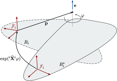
Figure 8: Screw motion of a rigid body represented by a body-fixed frame $\mathcal{F}_{i}$

The screw motion, with rotation angle $\varphi$, taking the body from its initial configuration $B_{i}$ to the final configuration $B_{i}^{\ast}$ is determined by the matrix exponential $\exp({{}^{i}}\widehat{\mathbf{X}}{{}^{i}}\varphi)$ of the matrix ${{}^{i}}\widehat{\mathbf{X}}{{}^{i}}$ defined as

$$\mathbf{X}=\left(\begin{array}[]{c}\mathbf{e}\\ \mathbf{p}\times\mathbf{e}+\mathbf{e}h\end{array}\right)\ \in{\mathbb{R}}^{6}\ \leftrightarrow\ \ \widehat{\mathbf{X}}=\left(\begin{array}[]{cc}\widetilde{\mathbf{e}}&\ \ \ \mathbf{p}\times\mathbf{e}+\mathbf{e}h\\ \mathbf{0}&0\end{array}\right)\in se\left(3\right).$$ (84)

The exponential mapping admits the closed form expression

$$\exp(\varphi\widehat{\mathbf{X}})=\left(\begin{array}[]{cc}\exp(\varphi\widetilde{\mathbf{e}})&\ \ \ (\mathbf{I}-\exp(\varphi\widetilde{\mathbf{e}}))\mathbf{p}+\varphi h\mathbf{e}\\ \mathbf{0}&1\end{array}\right),\ \text{for }h\neq\infty$$ (85)

where $\varphi$ is the rotation angle, and for pure translations, i.e. infinite pitch,

$$\exp(\varphi\widehat{\mathbf{X}})=\left(\begin{array}[]{cc}\mathbf{I}&\ \varphi\mathbf{e}\\ \mathbf{0}&1\end{array}\right),\ \text{for }h=\infty$$ (86)

where $\varphi$ is the translation variable. The exp mapping describes the frame transformation of a body-fixed frame from its final configuration to its initial configuration due to a screw motion where the screw coordinates are represented in the initial configuration. This is applicable to general frame transformations. Let ${{}^{i}}\mathbf{X}{{}^{i}}$ be the screw coordinates associated to the relative screw motion of body $j$ w.r.t. body $i$. The configuration of the body-fixed frame $\mathcal{F}_{j}$ relative to $\mathcal{F}_{i}$ is $\mathbf{C}_{i,j}=\exp({{}^{i}}\widehat{\mathbf{X}}{{}^{i}}\varphi)$, assuming that $\mathcal{F}_{j}$ and $\mathcal{F}_{i}$ initially overlap.

Notice the direction in which the frame transformation is indicated in fig. 8. The arc points toward the frame in which the screw coordinates are expressed.

Matrices of the form shown in (84) play obviously a key role as they give rise to frame transformations via the exp mapping. They form the Lie algebra $se\left(3\right)$. To any matrix $\widehat{\mathbf{X}}\in se\left(3\right)$ corresponds a unique vector $\mathbf{X}=(\mathbf{\xi},\mathbf{\eta})^{T}\in{\mathbb{R}}^{6}$ via the isomorphism (84). For simplicity also the notation $\exp\left(\mathbf{X}\varphi\right)$ is used instead of $\exp(\widehat{\mathbf{X}}\varphi)$.

Screws are geometric objects, thus frame invariant, and can be represented in any reference frame. Consider two frames $\mathcal{F}_{1}$ and $\mathcal{F}_{2}$ (fig. 9), and let ${{}^{2}}\mathbf{X}{{}^{2}}=\left({{}^{2}}\mathbf{e},{{}^{2}}\mathbf{p}_{2}\times{{}^{2}}\mathbf{e}+{{}^{2}}\mathbf{e}h\right)^{T}$ be screw coordinates measured and resolved in frame $\mathcal{F}_{2}$. That is, ${{}^{2}}\mathbf{e}$ is the unit vector along the axis resolved in $\mathcal{F}_{2}$, and ${{}^{2}}\mathbf{p}_{2}$ is the position vector $\overline{O_{2}P}$ of point $P$ on the axis resolved in $\mathcal{F}_{2}$. Let $S_{1,2}=\left(\mathbf{R}_{1,2},{{}^{1}}\mathbf{d}_{1,2}\right)$ be the transformation from $\mathcal{F}_{2}$ to $\mathcal{F}_{1}$. Then the screw coordinate vector measured and resolved in $\mathcal{F}_{1}$ is determined by ${{}^{1}\widehat{\mathbf{X}}^{1}}=\mathbf{S}_{1,2}{{}^{2}\widehat{\mathbf{X}}^{2}}\mathbf{S}_{1,2}^{-1}=\mathrm{Ad}_{\mathbf{S}_{1,2}}({{}^{2}\widehat{\mathbf{X}}^{2}})$, which reads in vector notation

$${{}^{1}\mathbf{X}^{1}}=\left(\begin{array}[]{c}{{}^{1}}\mathbf{e}\\ \ {{}^{1}}\mathbf{p}_{1}\times{{}^{1}}\mathbf{e}+{{}^{1}}\mathbf{e}h\end{array}\right)=\left(\begin{array}[]{cc}\mathbf{R}_{1,2}&\mathbf{0}\\ {{}^{1}}\widetilde{\mathbf{d}}_{1,2}\mathbf{R}_{1,2}&\mathbf{R}_{1,2}\end{array}\right)\left(\begin{array}[]{c}{{}^{2}}\mathbf{e}\\ \ {{}^{2}}\mathbf{p}_{2}\times{{}^{2}}\mathbf{e}+{{}^{2}}\mathbf{e}h\end{array}\right)=\mathbf{Ad}_{\mathbf{S}_{1,2}}{{}^{2}}\mathbf{X}{{}^{2}}$$ (87)

where ${{}^{1}}\mathbf{p}_{1}=\mathbf{R}_{1,2}{{}^{2}}\mathbf{p}_{2}+{{}^{1}}\mathbf{d}_{1,2}$ is the position vector $\overline{O_{1}P}$ of the point $P$ on the screw axis measured and resolved in $\mathcal{F}_{1}$. The transformation

$$\mathrm{Ad}_{\mathbf{C}}({\widehat{\mathbf{X}}})=\mathbf{C}{\widehat{\mathbf{X}}}\mathbf{C}^{-1}$$ (88)

with a general frame transformation $\mathbf{C}\in SE\left(3\right)$ is called the adjoined transformation LynchPark2017 ; Murray ; Selig . In vector notion this is

$$\mathbf{Ad}_{\mathbf{C}}=\left(\begin{array}[]{cc}\mathbf{R}&\mathbf{0}\\ \widetilde{\mathbf{r}}\mathbf{R}&\mathbf{R}\end{array}\right).$$ (89)

The terminology stems from the fact that $\mathbf{C}\in SE\left(3\right)$ describes a frame transformation, while $\mathbf{Ad}_{\mathbf{C}}$ describes the corresponding transformation of screw coordinates that belong to $se\left(3\right)$. It thus equally describes rigid body motions. It is used for instance in Bauchau2011 where $\mathbf{Ad}_{\mathbf{C}}$ is called the ’motion tensor’ and in Borri2001a where it is referred to as ’configuration tensor’ (and denoted with $\mathbf{C}$). If $\mathbf{C}_{i,j}$ is the configuration of body $j$ relative to body $i$, then $\mathbf{Ad}_{\mathbf{C}_{i,j}}$ transforms the coordinates of a screw represented in BFR on body $j$ to its coordinate representation in the BFR on body $i$.

For the product of transformations it holds

$$\mathbf{Ad}_{\mathbf{C}^{\prime}\mathbf{C}^{\prime\prime}}=\mathbf{Ad}_{\mathbf{C}^{\prime}}\mathbf{Ad}_{\mathbf{C}^{\prime\prime}}.$$ (90)

For sake of compactness, with slight abuse of notation the following notation is used

$$\mathbf{Ad}_{\mathbf{R}}=\left(\begin{array}[]{cc}\mathbf{R}&\mathbf{0}\\ \mathbf{0}&\mathbf{R}\end{array}\right),\ \text{for}\ \ C=\left(\mathbf{R},\mathbf{0}\right)\ \ \ \ \ \ \ \ \mathbf{Ad}_{\mathbf{r}}=\left(\begin{array}[]{cc}\mathbf{I}&\mathbf{0}\\ \widetilde{\mathbf{r}}&\mathbf{I}\end{array}\right),\ \text{for}\ \ C=\left(\mathbf{I},\mathbf{r}\right).$$ (91)

This allows for splitting the frame transformation (89) into the change of reference point followed by the change of basis as $\mathbf{Ad}_{\mathbf{C}}=\mathbf{Ad}_{\mathbf{r}}\mathbf{Ad}_{\mathbf{R}}$.

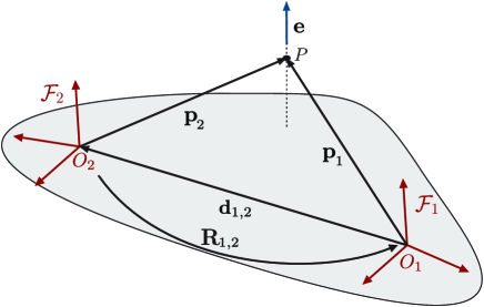
Figure 9: Frame transformation of screw coordinates according to $S_{1,2}=\left(\mathbf{R}_{1,2},{{}^{1}}\mathbf{d}_{1,2}\right)$.

A useful relation is that, for any $\widehat{\mathbf{X}}\in se\left(3\right)$ and $\mathbf{S}\in SE\left(3\right)$, it is

$$\mathbf{S}\exp(\widehat{\mathbf{X}})\mathbf{S}^{-1}=\exp(\mathbf{S}\widehat{\mathbf{X}}\mathbf{S}^{-1})=\exp(\mathrm{Ad}_{\mathbf{S}}(\widehat{\mathbf{X}})).$$ (92)

For constant $\mathbf{X}$ the derivative of the exponential is

$$\frac{\partial}{\partial t}\exp(t\widehat{\mathbf{X}})=\widehat{\mathbf{X}}\exp(t\widehat{\mathbf{X}})=\exp(t\widehat{\mathbf{X}})\widehat{\mathbf{X}}.$$ (93)

Notation:

The coordinate representation of a screw requires 1) a reference point from which the point on the screw axis is measured, and 2) a reference frame in which the vectors are resolved. The reference point is commonly the origin of a frame. These are indicated by the leading and trailing superscript, respectively. In (87) they were identical, but in general, ${{}^{i}\mathbf{X}^{j}}=\left({{}^{i}}\mathbf{e},{{}^{i}}\mathbf{p}_{j}\times{{}^{i}}\mathbf{e}+{{}^{i}}\mathbf{e}h\right)^{T}$ is the screw coordinate vector measured from the origin of $\mathcal{F}_{j}$ and resolved in $\mathcal{F}_{i}$. As apparent from (87) only screws measured and resolved in the same frame ($i=j$) are related by frame transformations. For sake of simplifying the notation, when $i=j$ the simplified notation ${{}^{i}\mathbf{X}}$ is used. The screw is then said to be represented in $\mathcal{F}_{i}$.

A.2 Twists as instantaneous Screw Motions – $se\left(3\right)$

The angular and translational velocity of a rigid body are summarized in the vector $\mathbf{V}=\left(\mathbf{\omega},\mathbf{v}\right)^{T}$ called the rigid body twist. This is a screw, and can hence be written as matrix of the form (84)

$$\widehat{\mathbf{V}}=\left(\begin{array}[]{cc}\widetilde{\mathbf{\omega}}&\mathbf{v}\\ \mathbf{0}&0\end{array}\right).$$ (94)

A general definition of twists requires specification of 1) the body of which the twist is measured, 2) the point at which the velocity is measured, and 3) the frame in which the velocity vectors are resolved. To this end, the following notion is used:

$${{}^{k}\mathbf{V}_{i}^{j}=}\left(\begin{array}[]{c}{{}^{k}}\mathbf{\omega}{{}_{i}}\\ {{}^{k}}\mathbf{v}{{}_{i}^{j}}\end{array}\right),\ \ \ \ \ \ \begin{array}[]{ll}i&\text{- index of the 'object' of which the twist is measured}\\ j&\text{- index of the frame in which the twist is measured}\\ k&\text{- index of the frame in which the vectors are resolved.}\end{array}$$ (95)

This is the twist of body $i$ measured in $\mathcal{F}_{j}$ and resolved in $\mathcal{F}_{k}$. More precisely ${{}^{k}}\mathbf{\omega}{{}_{i}}$ is the angular velocity of frame $\mathcal{F}_{i}$ measured and resolved in $\mathcal{F}_{k}$. Due to the translation invariance of the angular velocities it is independent from $\mathcal{F}_{j}$. The vector ${{}^{k}}\mathbf{v}{{}_{i}^{j}}$ is the translational velocity of the point on body $i$ that is instantaneously traveling trough the origin of $\mathcal{F}_{j}$ resolved in $\mathcal{F}_{k}$.

When $j=k$, the simplified notation ${{}^{k}\mathbf{V}_{i}}$ is used. A twist (and generally a screw) is said to be represented in frame $\mathcal{F}_{k}$ if it is measured and resolved in this frame, e.g. ${{}^{k}\mathbf{V}_{i}}$ is represented in frame $k$. The body-fixed and spatial representation of twists are most commonly used. The attribute ’body-fixed’ indicates that the frame in which the velocity is measured and resolved is the body-fixed RFR, i.e. $i=j=k$. ’Spatial’ is used when velocities are measured and resolved in the IFR, i.e. $j=k=0$. To further simplify the notation, the body-fixed and spatial twist of body $i$ is denoted by $\mathbf{V}_{i}^{\text{b}}=\left(\mathbf{\omega}_{i}^{\text{b}},\mathbf{v}_{i}^{\text{b}}\right)^{T}:={{}^{i}\mathbf{V}_{i}^{i}}$ and $\mathbf{V}_{i}^{\text{s}}=\left(\mathbf{\omega}_{i}^{\text{s}},\mathbf{v}_{i}^{\text{s}}\right)^{T}:={{}^{0}\mathbf{V}_{i}^{0}}$, respectively. The index 0 is omitted throughout the paper. For a body whose motion is described by $\mathbf{C}_{i}\left(t\right)$ according to (77) these are defined analytically by

$$\widehat{\mathbf{V}}_{i}^{\text{b}}=\left(\begin{array}[]{cc}\widetilde{\mathbf{\omega}}_{i}^{\text{b}}&\mathbf{v}_{i}^{\text{b}}\\ \mathbf{0}&0\end{array}\right)=\mathbf{C}_{i}^{-1}\dot{\mathbf{C}}_{i},\ \ \ \ \ \ \ \ \widehat{\mathbf{V}}_{i}^{\text{s}}=\left(\begin{array}[]{cc}\widetilde{\mathbf{\omega}}_{i}^{\text{s}}&\mathbf{v}_{i}^{\text{s}}\\ \mathbf{0}&0\end{array}\right)=\dot{\mathbf{C}}_{i}\mathbf{C}_{i}^{-1}.$$ (96)

Therein $\widetilde{\mathbf{\omega}}_{i}^{\text{b}}=\mathbf{R}_{i}^{T}\dot{\mathbf{R}}_{i}$ and $\widetilde{\mathbf{\omega}}_{i}^{\text{s}}=\dot{\mathbf{R}}_{i}\mathbf{R}_{i}^{T}$ define the body-fixed and spatial angular velocity. The vector $\mathbf{v}_{i}^{\text{b}}=\mathbf{R}_{i}^{T}\dot{\mathbf{r}}_{i}$ is the body-fixed translational velocity, i.e. the velocity of the origin of $\mathcal{F}_{i}$ measured in the IFR $\mathcal{F}_{0}$ and resolved in $\mathcal{F}_{i}$. The spatial translational velocity, $\mathbf{v}_{i}^{\text{s}}=\dot{\mathbf{r}}_{i}+\mathbf{r}_{i}\times\mathbf{\omega}_{i}^{\text{s}}$, is the velocity of the point of the body that is momentarily passing through the origin of the IFR $\mathcal{F}_{0}$ resolved in the IFR.

Twists represented in different frames transform as screws according to (89). Let ${{}^{1}\mathbf{V}_{i}^{1}}=\left({{}^{1}}\mathbf{\omega}{{}_{i}},{{}^{1}}\mathbf{v}{{}_{i}^{1}}\right)^{T}$ be the twist of body $i$ represented in a frame $\mathcal{F}_{1}$. Let $S_{21}=\left(\mathbf{R}_{21},{{}^{2}}\mathbf{r}{{}_{21}}\right)$ be the frame transformation from $\mathcal{F}_{1}$ to another frame $\mathcal{F}_{2}$. Then ${{}^{2}\mathbf{V}_{i}^{2}}=\mathbf{Ad}_{\mathbf{S}_{21}}{{}^{1}\mathbf{V}_{i}^{1}}$ is the twist of body $i$ represented in $\mathcal{F}_{2}$. This is ${{}^{2}\mathbf{V}_{i}^{2}}=\left({{}^{2}}\mathbf{\omega}{{}_{i}},{{}^{2}}\mathbf{v}{{}_{i}^{2}}\right)^{T}$, where ${{}^{2}}\mathbf{v}{{}_{i}^{2}}={{}^{2}}\mathbf{v}{{}_{i}^{1}}+{{}^{2}}\mathbf{r}{{}_{21}}\times{{}^{2}}\mathbf{\omega}{{}_{i}}$ is the translational velocity of the point of body $i$ traveling through the origin of $\mathcal{F}_{2}$, with ${{}^{2}}\mathbf{v}{{}_{i}^{1}}=\mathbf{R}_{21}{{}^{1}}\mathbf{v}{{}_{i}^{1}}$ and ${{}^{2}}\mathbf{\omega}{{}_{i}}=\mathbf{R}_{21}{{}^{1}}\mathbf{\omega}{{}_{i}}$. The twist is represented, i.e. measured and resolved, in $\mathcal{F}_{2}$. The vector components can be resolved in yet another frame $\mathcal{F}_{3}$. If $\mathbf{R}_{32}$ is the rotation matrix of this change of coordinates, then ${{}^{3}\mathbf{V}_{i}^{2}}=\mathbf{Ad}_{\mathbf{R}_{32}}{{}^{2}\mathbf{V}_{i}^{2}}$, with (91), is the twist measured in $\mathcal{F}_{2}$ but resolved in $\mathcal{F}_{3}$: ${{}^{3}\mathbf{V}_{i}^{2}}=\left({{}^{3}}\mathbf{\omega}{{}_{i}},{{}^{3}}\mathbf{v}{{}_{i}^{2}}\right)^{T}$, with ${{}^{3}}\mathbf{\omega}{{}_{i}}=\mathbf{R}_{32}{{}^{2}}\mathbf{\omega}{{}_{i},^{3}}\mathbf{v}{{}_{i}^{2}}=\mathbf{R}_{32}{{}^{2}}\mathbf{v}{{}_{i}^{2}}={{}^{3}}\mathbf{v}{{}_{i}^{1}}+{{}^{3}}\mathbf{r}{{}_{21}}\times{{}^{3}}\mathbf{\omega}{{}_{i}}$. This is indeed not a frame transformation but rather a coordinate transformation. Only if twists are measured and resolved in the same frame, like body-fixed and spatial twists, the screw coordinate transformation is a frame transformation. In particular, $\mathbf{V}_{i}^{\text{s}}=\mathbf{Ad}_{\mathbf{C}_{i}}\mathbf{V}_{i}^{\text{b}}$.

The relative twist of body $j$ w.r.t. body $i$, i.e. the twist of $\mathcal{F}_{i}$ represented in $\mathcal{F}_{j}$, is readily defined as ${{}^{j}\widehat{{\mathbf{V}}}_{i}}=\dot{\mathbf{C}}_{j,i}\mathbf{C}_{j,i}^{-1}$. With (79) and (88) this is

$${{}^{j}\widehat{{\mathbf{V}}}_{i}} = \frac{d}{dt}\left(\mathbf{C}_{j}^{-1}\mathbf{C}_{i}\right)\mathbf{C}_{i}^{-1}\mathbf{C}_{j}=\mathbf{C}_{j}^{-1}\dot{\mathbf{C}}_{i}\mathbf{C}_{i}^{-1}\mathbf{C}_{j}-\mathbf{C}_{j}^{-1}\dot{\mathbf{C}}_{j}\mathbf{C}_{j}^{-1}\mathbf{C}_{j}$$ (97)

$$= \mathrm{Ad}_{\mathbf{C}_{j}}^{-1}({\widehat{{\mathbf{V}}}_{i}^{\text{s}}}-{\widehat{{\mathbf{V}}}_{j}^{\text{s}})}=\mathrm{Ad}_{\mathbf{C}_{j}}^{-1}({\widehat{{\mathbf{V}}}_{i}^{\text{s}})-\widehat{{\mathbf{V}}}_{j}^{\text{b}}}.$$

This is the difference of the twists of the two bodies represented in the BFR at body $j$.

There are yet two further forms of twist used in MBS kinematics. In the hybrid form, denoted with $\mathbf{V}_{i}^{\text{h}}=\left(\mathbf{\omega}_{i}^{\text{s}},\dot{\mathbf{r}}_{i}\right)^{T}={{}^{0}{\mathbf{V}}_{i}^{i}}$, the twist of body $i$ is measured in the body-fixed frame $\mathcal{F}_{i}$ but resolved in the IFR $\mathcal{F}_{0}$. The mixed form of twists, denoted with $\mathbf{V}_{i}^{\text{m}}=\left(\mathbf{\omega}_{i}^{\text{b}},\dot{\mathbf{r}}_{i}\right)^{T}$, uses the body-fixed angular velocity $\mathbf{\omega}_{i}^{\text{b}}$ and the translational velocity $\dot{\mathbf{r}}_{i}$. The two forms are related by

$$\mathbf{V}_{i}^{\text{m}}=\left(\begin{array}[]{cc}\mathbf{R}_{i}^{T}&\mathbf{0}\\ \mathbf{0}&\mathbf{I}\end{array}\right)\mathbf{V}_{i}^{\text{h}}=\left(\begin{array}[]{cc}\mathbf{I}&\mathbf{0}\\ \mathbf{0}&\mathbf{R}_{i}\end{array}\right)\mathbf{V}_{i}^{\text{b}}=\left(\begin{array}[]{cc}\mathbf{R}_{i}^{T}&\mathbf{0}\\ -\widetilde{\mathbf{r}}_{i}&\mathbf{I}\end{array}\right)\mathbf{V}_{i}^{\text{s}}.$$ (98)

These transformations are apparently not frame transformations (that would be described by the adjoint mapping). The definition of twists are summarized in table 4.

	Reference point is origin of	Frame to resolve angular velocity	Frame to resolve translational velocity
$\mathbf{V}_{i}^{\text{s}}$	IFR	IFR	IFR
$\mathbf{V}_{i}^{\text{b}}$	BFR	BFR	BFR
$\mathbf{V}_{i}^{\text{h}}$	BFR	IFR	IFR
$\mathbf{V}_{i}^{\text{m}}$	BFR	BFR	IFR

Table 4: Summary of the reference point at which the translational velocity is measured, and the frame in which the angular respectively translational velocity is resolved

Remark 17

It is should be remarked that also the hybrid and mixed twists can be derived analytically by left and right trivialization, as in (96), if rigid body motions are not considered to be elements of $SE\left(3\right)$. To this end, the direct product group $SO\left(3\right)\times{\mathbb{R}}^{3}$ is used as configuration space of a rigid body: $C=\left(\mathbf{R},\mathbf{r}\right)\in SO\left(3\right)\times{\mathbb{R}}^{3}$. The multiplication in this group is $C_{1}\cdot C_{2}=(\mathbf{R}_{1}\mathbf{R}_{2},\mathbf{r}_{1}+\mathbf{r}_{2})$. This is clearly not a frame transformation. The hybrid and mixed twist are then $\mathbf{V}^{\text{m}}=C^{-1}\cdot\dot{C}=(\mathbf{\omega}^{\text{b}},\dot{\mathbf{r}})$ and $\mathbf{V}^{\text{h}}=\dot{C}\cdot C^{-1}=(\mathbf{\omega}^{\text{s}},\dot{\mathbf{r}})\in so\left(3\right)\times\mathbb{R}^{3}$. It must be emphasized that the direct product group does not represent screw motions. Even though it is occasionally used to model MBS and also in Lie group integration schemes.

B Nomenclature

Symbols:

$\mathcal{F}_{0}$	- Inertial reference frame (IFR)
$\mathcal{F}_{i}$	- Body-fixed reference frame (BFR) of body $i$
$\mathcal{J}_{i,i}$	- Body-fixed joint frame (JFR) for joint $i$ at body $i$
	joint $i$ connects body $i$ with its predecessor body $i-1$
$\mathcal{J}_{i-1,i}$	- JFR for joint $i$ at body $i-1$
${{}^{i}}\mathbf{r}$	- Coordinate representation of a vector resolved in BFR on body $i$.
	The index is omitted if this is the IFR: $\mathbf{r}\equiv{{}^{0}}\mathbf{r}$.
$\mathbf{R}_{i}$	- Rotation matrix from BFR $\mathcal{F}_{i}$ at body $i$ to IFR $\mathcal{F}_{0}$
$\mathbf{R}_{i,j}$	- Rotation matrix transforming coordinates resolved in BFR $\mathcal{F}_{j}$
	to coordinates resolved in $\mathcal{F}_{i}$
$\mathbf{r}_{i}$	- Position vector of origin of BFR $\mathcal{F}_{i}$ at body $i$ resolved in IFR $\mathcal{F}_{0}$
$\mathbf{r}_{i,j}$	- Position vector from origin of BFR $\mathcal{F}_{i}$ to origin of BFR $\mathcal{F}_{j}$
$\widetilde{\mathbf{x}}$	- skew symmetric matrix associated to the vector $\mathbf{x}\in{\mathbb{R}}^{3}$
$C_{i}=\left(\mathbf{R}_{i},\mathbf{r}_{i}\right)$	- Absolute configuration of body $i$. This is denoted in matrix form with $\mathbf{C}_{i}$
$\mathbf{C}_{i,j}=\mathbf{C}_{i}^{-1}\mathbf{C}_{j}$	- Relative configuration of body $j$ w.r.t. body $i$
${{}^{k}}\mathbf{v}{{}_{i}^{j}}$	- Translational velocity of body $i$ measured at origin of BFR $\mathcal{F}_{j}$, resolved in BFR $\mathcal{F}_{k}$
$\mathbf{v}_{i}^{\text{b}}\equiv{{}^{i}}\mathbf{v}{{}_{i}^{i}}$	- Body-fixed representation of the translational velocity of body $i$
$\mathbf{v}_{i}^{\text{s}}\equiv{{}^{0}}\mathbf{v}{{}_{i}^{0}}$	- Spatial representation of the translational velocity of body $i$
${{}^{k}}\mathbf{\omega}{{}_{i}}$	- Angular velocity of body $i$ measured and resolved in BFR $\mathcal{F}_{k}$
$\mathbf{\omega}{{}_{i}^{\text{b}}}\equiv{{}^{i}}\mathbf{\omega}{{}_{i}}$	- Body-fixed representation of the angular velocity of body $i$
$\mathbf{\omega}{{}_{i}^{\text{s}}}\equiv{{}^{0}}\mathbf{\omega}{{}_{i}}$	- Spatial representation of the angular velocity of body $i$
${{}^{k}}\mathbf{V}{{}_{i}^{j}}$	- Twist of (RFR of) body $i$ measured in $\mathcal{F}_{j}$ and resolved in $\mathcal{F}_{k}$
$\mathbf{V}_{i}^{\text{b}}\equiv{{}^{i}}\mathbf{V}{{}_{i}^{i}}$	- Body-fixed representation of the twist of body $i$
$\mathbf{V}{{}_{i}^{\text{s}}}\equiv{{}^{0}}\mathbf{V}{{}_{i}^{0}}$	- Spatial representation of the twist of body $i$
$\mathbf{V}_{i}^{\text{h}}\equiv{{}^{0}}\mathbf{V}{{}_{i}^{i}}$	- Hybrid form of the twist of body $i$
$\mathsf{V}{{}^{\text{b}}}$	- Vector of system twists in body-fixed representation
$\mathsf{V}{{}^{\text{s}}}$	- Vector of system twists in spatial representation
$\mathsf{V}{{}^{\text{h}}}$	- Vector of system twists in hybrid representation
$\mathsf{V}{{}^{\text{m}}}$	- Vector of system twists in mixed representation
$\mathbf{Ad}_{\mathbf{R}}$	- Screw transformation associated with $C=\left(\mathbf{R},\mathbf{0}\right)$
$\mathbf{Ad}_{\mathbf{r}}$	- Screw transformation associated with $C=\left(\mathbf{I},\mathbf{r}\right)$
$\mathbf{Ad}_{\mathbf{C}_{i,j}}$	- Transformation matrix transforming screw coordinates represented in $\mathcal{F}_{j}$
	to screw coordinates represented in $\mathcal{F}_{i}$
$\widehat{\mathbf{X}}\in se\left(3\right)$	- $4\times 4$ matrix associated with the screw coordinate vectors $\mathbf{X}\in{\mathbb{R}}^{6}$
$SE\left(3\right)$	- Special Euclidean group in three dimensions – Lie group of rigid body motions
$se\left(3\right)$	- Lie algebra of $SE\left(3\right)$ – algebra of screws
$\mathbf{q}\in{\mathbb{V}}^{n}$	- Joint coordinate vector
${\mathbb{V}}^{n}$	- Configuration space

Joint Screw Coordinates:

The introduction of joint screw coordinates requires specification of a frame in which the screw is measured and a frame where the coordinates are solved. To this end, the following notation for screw coordinates is used:

$${{}^{k}\mathbf{X}_{i}^{j}},\ \ \ \ \ \ \begin{array}[]{ll}i&\text{- index of joint}\\ j&\text{- index of frame in which the joint screw is measured}\\ k&\text{- index of frame in which the coordinates are resolved}\end{array}$$

A screw is said to be represented in frame $j$ if $j=k$. To simplify the notation the following short hand notation is used: ${{}^{j}\mathbf{X}_{i}}:={{}^{j}}\mathbf{X}{{}_{i}^{j}},\ \mathbf{X}{{}_{i}}:={{}^{0}}\mathbf{X}{{}_{i}}{{}^{0}}$.

${}^{i-1}\mathbf{Z}_{i}$	- Constant screw coordinate vector of joint $i$ represented in JFR $\mathcal{J}_{i-1,i}$ at body $i-1$,
	determined in the reference configuration $\mathbf{q}=\mathbf{0}$
${{}^{i}}\mathbf{X}_{i}$	- Constant screw coordinate vector of joint $i$ represented in BFR $\mathcal{F}_{i}$ at body $i$,
	determined in the reference configuration $\mathbf{q}=\mathbf{0}$
${{}^{i-1}}\bar{\mathbf{X}}_{i}$	- Constant screw coordinate vector of joint $i$ represented in BFR $\mathcal{F}_{i-1}$ at body $i-1$,
	determined in the reference configuration $\mathbf{q}=\mathbf{0}$
$\mathbf{Y}_{i}$	- Constant screw coordinate vector of joint $i$ represented in IFR $\mathcal{F}_{0}$,
	determined in the reference configuration $\mathbf{q}=\mathbf{0}$
${{}^{0}}\mathbf{X}_{i}^{i}$	- Instantaneous screw coordinate vector of joint $i$ measured in BFR $\mathcal{F}_{i}$
	but resolved in IFR $\mathcal{F}_{0}$

Representations of Velocity of Rigid Body $i$:

Body-fixed twist:	$\mathbf{V}_{i}^{\text{b}}=\left(\begin{array}[]{c}\mathbf{\omega}_{i}^{\text{b}}\\ \mathbf{v}_{i}^{\text{b}}\end{array}\right),$ with $\widetilde{\mathbf{\omega}}_{i}^{\text{b}}:={{}^{i}}\widetilde{\mathbf{\omega}}{{}_{i}}=\mathbf{R}_{i}^{T}\dot{\mathbf{R}}_{i},\mathbf{v}_{i}^{\text{b}}:={{}^{i}}\mathbf{v}{{}_{i}^{i}}=\mathbf{R}_{i}^{T}\dot{\mathbf{r}}_{i}$
	Twist represented in BFR $\mathcal{F}_{i}$, i.e. measured and resolved in $\mathcal{F}_{i}$
Spatial twist:	$\mathbf{V}_{i}^{\text{s}}=\left(\begin{array}[]{c}\mathbf{\omega}_{i}^{\text{s}}\\ \mathbf{v}_{i}^{\text{s}}\end{array}\right),$ with $\widetilde{\mathbf{\omega}}_{i}^{\text{s}}:={{}^{0}\widetilde{\mathbf{\omega}}{{}_{i}}}=\dot{\mathbf{R}}_{i}\mathbf{R}_{i}^{T},\mathbf{v}_{i}^{\text{s}}:={{}^{0}}\mathbf{v}{{}_{i}^{0}}=\dot{\mathbf{r}}_{i}-\widetilde{\mathbf{\omega}}{{}_{i}^{\text{s}}}\mathbf{r}_{i}$
	Twist represented in IFR $\mathcal{F}_{0}$, i.e. measured and resolved in $\mathcal{F}_{0}$
Hybrid twist:	$\mathbf{V}_{i}^{\text{h}}=\left(\begin{array}[]{c}\mathbf{\omega}_{i}^{\text{s}}\\ \dot{\mathbf{r}}_{i}\end{array}\right)$
	Twist measured in BFR $\mathcal{F}_{i}$ but resolved in IFR $\mathcal{F}_{0}$
Mixed twist:	$\mathbf{V}_{i}^{\text{m}}=\left(\begin{array}[]{c}\mathbf{\omega}_{i}^{\text{b}}\\ \dot{\mathbf{r}}_{i}\end{array}\right)$
	Angular velocity is measured and resolved in BFR $\mathcal{F}_{i}$. Translational velocity is measured in BFR $\mathcal{F}_{i}$ but resolved in IFR $\mathcal{F}_{0}$.

References

- (1) K. Anderson: An Order n Formulation for the Motion Simulation of General Multi-Rigid-Body Constrained Systems, Computers & Structures, Vol. 43, No. 3, 1992, pp. 565-579
- (2) K.S. Anderson, J.H. Critchley: Improved ‘Order-N’ Performance Algorithm for the Simulation of Constrained Multi-Rigid-Body Dynamic Systems, Multibody System Dynamics, Vol. 9, No. 2, 2003, pp 185-212
- (3) K.S. Anderson, Y. Hsu: Order-(n +m) direct differentiation determination of design sensitivity for constrained multibody dynamic systems, Struct Multidisc Optim, Vol. 26, 2004, pp. 171-182
- (4) J. Angeles: Rational Kinematics, Springer, NY, 1988
- (5) J. Angles, S. Lee: The formulation of dynamical equations of holonomic mechanical systems using a natural orthogonal complement, ASME J. Appl. Mech., Vol. 55, 1988, pp. 243-244
- (6) J. Angeles: Fundamentals of robotic mechanical systems - second edition, Springer, 2003
- (7) D.S. Bae, R.S. Hwang, E.J. Haug: A Recursive Formulation for Real-Time Dynamic Simulation of Mechanical Systems, ASME Journal of Mechanical Design, Vol. 113, No. 2, 1988, pp. 158-166
- (8) D. S. Bae et al.: A generalized recursive formulation for constrained flexible multibody dynamics, Int. J. Numer. Meth. Engng, Vol. 50, 2001, pp. 1841–1859
- (9) O. Bauchau: Flexible Multibody Dynamics, Springer, Dordrecht, Heidelberg, London, New-York, 2011
- (10) B. Bongardt, F. Kirchner: Newton–Euler equations in general coordinates, Proc. of Mathematics of Robotics (IMA), September 9-11, 2015, St Anne’s College, University of Oxford
- (11) B. Bongardt: Analytical approaches for design and operation of haptic human-machine interfaces, PhD thesis, University Bremen, 2015
- (12) W.J. Book: Recursive Lagrangian Dynamics of Flexible Manipulator Arms, Int. J. of Robotics Research, Vol. 3, No. 3, 1984, pp. 87-101
- (13) M. Borri, C.L. Bottasso, L. Trainelli: Integration of Elastic Multibody Systems by Invariant Conserving/Dissipating Algorithms - Part I : Formulation Computer Methods in Applied Mechanics and Engineering, Vol. 190 (29/30), 2001, pp. 3669-3699
- (14) M. Borri, C.L. Bottasso, L. Trainelli: Integration of Elastic Multibody Systems by Invariant Conserving/Dissipating Algorithms - Part II : Numerical Schemes and Applications Computer Methods in Applied Mechanics and Engineering, Vol. 190 (29/30), 2001, pp. 3701-3733
- (15) M. Borri, C.L. Bottasso, L. Trainelli: An Invariant-Preserving Approach to Robust Finite-Element Multibody Simulation Zeitschrift für Angewandte Mathematik und Mechanik, Vol. 83 (10), 2003, pp. 663-676
- (16) C.L. Bottasso, M. Borri: Integrating finite rotations, Comput. Methods Appl. Mech. Engrg., Vol. 164, 1998, pp. 307-331
- (17) O. Bottema, B. Roth: Theoretical Kinematics. Dover Publications, 1990
- (18) H. Bremer: Elastic Multibody Dynamics, Springer, 2010
- (19) R. W. Brockett: Robotic manipulators and the product of exponentials formula, Mathematical Theory of Networks and Systems, Lecture Notes in Control and Information Sciences Vol. 58, 1984, pp 120-129
- (20) R. W. Brockett, A. Stokes, F. Park: A geometrical formulation of the dynamical equations describing kinematic chains, IEEE Int. Conf. Robotics and Automation (ICRA), 1993, Vol.2, 637 - 641
- (21) O. Brüls, A. Cardona, M. Arnold: Lie group generalized-alpha time integration of constrained flexible multibody systems, Mech. Mach. Theory, Vol. 48, 2012, pp. 121-137
- (22) H. Bruyninckx, J. De Schutter: Symbolic differentiation of the velocity mapping for a serial kinematic chain, Mech. Mach. Theory, Vol. 31, No. 2, 1996, pp. 135-148
- (23) D.P. Chevallier: Lie Algebras, Modules, Dual Quaternions and algebraic Methods in Kinematics, Mech. Mach. Theory, Vol. 26, No. 6, 1991, pp. 613-627
- (24) D.P. Chevallier: Lie Groups and Multibody Dynamics Formalism, Proc. EUROMECH Colloquium 320, Prague, 1994, pp. 1-20
- (25) J.H. Critchley, K.S. Anderson: A generalized recursive coordinate reduction meethod for multibody system dynamics, Int. J. for Multiscale Computational Eng., Vol. 1, no. 2&3, 2003, pp. 181-199
- (26) J. Denavit, R. Hartenberg: A kinematic notation for lower-pair mechanisms based on matrices, Journal of Applied Mechanics, Vol. 22, 1955, pp. 215-221
- (27) R. Featherstone: The Calculation of Robot Dynamics using Articulated-Body Inertias, Int. J. Robotics Research, Vol. 2, No. 1, 1983, pp. 13-30
- (28) R. Featherstone: Rigid Body Dynamics Algorithms, Springer, 2008
- (29) A. Fijany: Parallel O(1og N) Algorithms for Computation of Manipulator Forward Dynamics, IEEE Trans. Rob. and Automat., Vol. 11, No. 3, 1995, pp. 389-400
- (30) J. Gallardo, J.M. Rico, A. Frisoli, D. Checcacci, M. Bergamasco: Dynamics of parallel manipulators by means of screw theory, Mech. Mach. Theory, Vol. 38, No. 11, 2003, pp. 1113-1131
- (31) K.C. Gupta: Kinematic Analysis of Manipulators Using the Zero Reference Position Description, The International Journal of Robotics Research 1986, Vol. 5, No. 2, 1986
- (32) J.M. Hervé: Analyse Structurelle des Mécanismes par Groupe des Déplacements, Mech. Mach. Theory, Vol. 13, 1978, pp. 437-450
- (33) J.M. Hervé: Intrinsic formulation of problems of geometry and kinematics of mechanisms, Mech. Mach. Theory, Vol. 17, No. 3, 1982, pp. 179-184
- (34) J.M. Hollerbach: A Recursive Lagrangian Formulation of Maniputator Dynamics and a Comparative Study of Dynamics Formulation Complexity, IEEE Tran. Systems, Man, Cyb., Vol. SMC-10, No. 11, 1980, pp. 730-736
- (35) K.H. Hunt: Kinematic Geometry of Mechanisms, Oxford Engineering Science Series, Oxford, 1990
- (36) A. Jain: Unified Formulation of Dynamics for Serial Rigid Multibody Systems, Journal of Guidance, Control and Dynamics, Vol. 14, No. 3, 1991, pp. 531-542
- (37) A. Jain, G. Rodriguez: Diagonalized Lagrangian robot dynamics, IEEE Trans. Rob. and Automat., Vol. 11, No. 4, 1995, pp. 971-584
- (38) A. Jain: Graph theoretic foundations of multibody dynamics, Part I: structural properties, Multibody Syst Dyn., Vol. 26, 2011, pp. 307-333
- (39) W. Khalil, J.F. Kleinfinger: A New Geometric Notation for Open and Closed-Loop Robots. In: Proceedings of the IEEE International Conference on Robotics and Automation, 1986, S. 1174-1179
- (40) G. Legnani: A homogeneous matrix approach to 3D kinematics and dynamics–I. Theory, Mech. Mach. Theory, Vol. 31, No. 5, 1996, pp. 573–587
- (41) G. Legnani: A homogeneous matrix approach to 3D kinematics and dynamics–II. Applications to chains of rigid bodies and serial manipulators, Mech. Mach. Theory, Vol. 31, No. 5, 1996, pp. 589-605
- (42) W. Lilly, D.E. Orin: Alternate Formulations for the Manipulator Inertia Matrix, Int. J. Rob. Res., Vol. 10, No. 1, 1991, pp. 64-74
- (43) Y. Liu: Screw-matrix method in dynamics of multibody systems, Acta Mechanica Sinica, Vol. 4, No. 2, 1988, pp. 165-174
- (44) K.M. Lynch, F.C. Park: Modern Robotics, Cambridge, 2017
- (45) P. Maißer: Analytische Dynamik von Mehrkörpersystemen, Journal of Applied Mathematics and Mechanics / Zeitschrift für Angewandte Mathematik und Mechanik (ZAMM), Vol. 68, No. 10, 1988, pp. 463-481
- (46) P. Maisser: Differential-geometric methods in multibody dynamics, Nonlinear Anal. Theory Methods Appl., 1997, Vol. 30, No. 8, pp. 5127-5133
- (47) J.M. McCarthy, An Introduction to Theoretical Kinematics MIT Press, Cambridge, Mass. 1990
- (48) C.D. Mladenova: Group Theory in the Problems of Modeling and Control of Multi-Body Systems, Journal of Geometry and Symmetry in Physics, Vol. 8, 2006, pp. 17-121
- (49) A. Müller: Representation of the Kinematic Topology of Mechanisms for Kinematic Analysis, Mechanical Sciences, Vol. 6, pp. 1-10, 2015
- (50) A. Müller, P. Maisser: Lie group formulation of kinematics and dynamics of constrained MBS and its application to analytical mechanics, Multibody System Dynamics, Vol. 9, 2003, pp. 311-352
- (51) A. Müller: Implementation of a Geometric Constraint Regularization for Multibody System Models, Archive of Mechanical Engineering, Vol. 61, No. 2, 2014, pp. 376-383
- (52) A. Müller, Z. Terze: The significance of the configuration space Lie group for the constraint satisfaction in numerical time integration of multibody systems, Mechanism and Machine Theory, Vol. 82, 2014, pp. 173-202
- (53) A. Müller: A Note on the Motion Representation and Configuration Update in Time Stepping Schemes for the Constrained Rigid Body, BIT Numerical Mathematics, Vol. 56, No. 3, 2016
- (54) A. Müller: Screw and Lie Group Theory in Multibody Dynamics –Recursive Algorithms and Equations of Motion of Tree-Topology Systems, submitted to Multibody System Dynamics, 2016
- (55) A. Müller: Coordinate Mappings for Rigid Body Motions, ASME Journal of Computational and Nonlinear Dynamics, Vol. 12, No. 2, 2016
- (56) R.M. Murray, Z. Li, and S.S. Sastry, A Mathematical Introduction to Robotic Manipulation, CRC Press Boca Raton, 1994
- (57) J. Naudet, D. Lefeber, F. Daerden, Z. Terze: Forward Dynamics of Open-Loop Multibody Mechanisms Using an Efficient Recursive Algorithm Based on Canonical Momenta, Multibody System Dynamics, Vol. 10, No. 1, 2003, pp. 45-59
- (58) D. Orin, et al.: Kinematic and Kinetic Analysis of Open-Chain linkages Utilizing Newton-Euler Methods, Math. Biosciences, Vol. 43, 1979, pp. 107-130
- (59) D. Orin, W. Schrader: Efficient computation of the Jacobian for robot manipulators, Int. J. Robotics Research, Vol. 3, No. 4, 1984
- (60) F.C. Park: Computational Aspects of the Product-of-Exponentials Formula for Robot Kinematics, IEEE Trans. Aut. Contr, Vol. 39, No. 3, 1994, 643-647
- (61) F. C. Park, J. E. Bobrow, S. R. Ploen: A Lie group formulation of robot dynamics, Int. J. Rob. Research, Vol. 14, No. 6, 1995, pp. 609-618
- (62) F.C. Park, M.W. Kim: Lie theory, Riemannian geometry, and the dynamics of coupled rigid bodies, Z. angew. Math. Phys., Vol. 51, 2000, pp. 820-834
- (63) S.R. Ploen, F.C. Park: A Lie group formulation of the dynamics of cooperating robot systems, Rob. and Auton. Sys., Vol. 21, 1997, pp. 279-287
- (64) S.R. Ploen, F.C. Park: Coordinate-Invariant Algorithms for Robot Dynamics, IEEE Tran. Rob. Aut., Vol. 15, No. 6, 1999, pp. 1130-1135
- (65) F. Reuleaux: Theoretische Kinematik: Grundzüge einer Theorie des Maschinenwesens, Vieweg, Braunschweig, 1875
- (66) F. Reuleaux: Kinematics of machinery, Dover, NY, 1963
- (67) G. Rodriguez: Kalman Filtering, Smoothing, and ecursive Robot Arm Forward and Inverse Dynamics, IEEE J. Rob. and Automation, Vol. RA-3, No. 6, 1987, pp. 624-639
- (68) G. Rodriguez, A. Jain, K. Kreutz-Delgado: A Spatial Operator Algebra for Manipulator Modelling and Control, Int. J. Robotics Research, Vol. 10, No. 4, 1991, pp. 371-381
- (69) G. Rodriguez, A. Jain, K. Kreutz-Delgado: Spatial Operator Algebra for Multibody System Dynamics, J. Astron Sciences, Vol. 40, 1992, pp. 27-50
- (70) A.E. Samuel, P.R. McAree, K.H. Hunt: Unifying Screw Geometry and Matrix Transformations, Int. J. Rob. Research, Vol. 10, No. 5, 1991, pp. 454-472
- (71) J. Selig: Geometric Fundamentals of Robotics (Monographs in Computer Science Series), Springer-Verlag New York, 2005
- (72) A.A. Shabana: Dynamics of Multibody Systems 4th ed., Springer, 2013
- (73) P.N. Sheth, J.J. Uicker: A Generalized Symbolic Notation for Mechanisms, J. Eng. Ind, Vol. 93, No. 1, 1971, pp. 102-112
- (74) J.C. Simo, L. Vu-Quoc: On the Dynamics in Space of Rods Undergoing Undergoing Large Motions – Geometrically Exact Approach,’ Comput. Methods Appl. Mech. Eng., Vol. 66, 1986, pp. 125-161
- (75) J.C. Simo, K.K. Wong: Unconditionally Stable Algorithms for Rigid Body Dynamics That Exactly Preserve Energy and Momentum,’ Int. J. Numer. Methods Eng., Vol. 31, No. 1, 1991, pp. 19-52
- (76) V. Sonneville, A. Cardona and O. Bruls. Geometrically exact beam finite element formulated on the special Euclidean group SE(3), Computer Methods in Applied Mechanics and Engineering, 2014, Vol. 268, pp. 451-474
- (77) W. Stelzle, A. Kecskeméthy, M. Hiller: A comparative study of recursive methods, Archive of Applied Mechanics, Vol. 66, 1995, pp. 9-19
- (78) J.J. Uicker, B. Ravani, P.N. Sheth: Matrix Methods in the Design Analysis of Mechanisms and Multibody Systems, Cambridge University Press, 2013
- (79) M. Vukobratović, V. Potkonjak: Contribution of the forming of computer methods for automatic modelling of spatial mechanisms motions, Mechanism and Machine Theory, Vol. 14, No. 3, 1979, pp. 179-188
- (80) K.J. Waldron: Geometrically based manipulator rate control algorithms. Mechanism and Machine Theory, Vol. 17, No. 6, 1982, pp. 379-385
- (81) J. S. Won, S. W. Choi, W. Peine: Curved RCM of Surgical Robot Arm, Patent WO 2009/104853 A1, Aug. 27, 2009
- (82) D. E. Whitney: The Mathematics of Coordinated Control of Prosthetic Arms and Manipulators, Trans. ASME J. Dyn. Sys., Meas., Control, Vol. 94, No. 4, 1972, pp. 303-309
- (83) K. Yamane, Y. Nakamura: Comparative Study on Serial and Parallel Forward Dynamics Algorithms for Kinematic Chains, Int. J. Rob. Res., Vol. 28, 2009, pp. 622-629