Testing Multi-Subroutine Quantum Programs: From Unit Testing to Integration Testing

Abstract.

Quantum computing has emerged as a promising field with the potential to revolutionize various domains by harnessing the principles of quantum mechanics. As quantum hardware and algorithms continue to advance, the development of high-quality quantum software has become crucial. However, testing quantum programs poses unique challenges due to the distinctive characteristics of quantum systems and the complexity of multi-subroutine programs. In this paper, we address the specific testing requirements of multi-subroutine quantum programs. We begin by investigating critical properties through a survey of existing quantum libraries, providing insights into the challenges associated with testing these programs. Building upon this understanding, we present a systematic testing process tailored to the intricacies of quantum programming. The process covers unit testing and integration testing, with a focus on aspects such as IO analysis, quantum relation checking, structural testing, behavior testing, and test case generation. We also introduce novel testing principles and criteria to guide the testing process. To evaluate our proposed approach, we conduct comprehensive testing on typical quantum subroutines, including diverse mutations and randomized inputs. The analysis of failures provides valuable insights into the effectiveness of our testing methodology. Additionally, we present case studies on representative multi-subroutine quantum programs, demonstrating the practical application and effectiveness of our proposed testing processes, principles, and criteria.

1. Introduction

Quantum computing is a rapidly evolving field with great potential for advancements in various domains (national2019quantum, ). It leverages the principles of quantum mechanics to process information and perform computational tasks. Quantum algorithms, in comparison to classical algorithms, offer the promise of accelerated solutions for specific problems (deutsch1985quantum, ; grover1996fast, ; shor1999polynomial, ). As quantum hardware devices and algorithms continue to advance, developing high-quality quantum software has become increasingly crucial.

In recent years, several quantum programming languages have been proposed, including Q#(svore2018q, ), Qiskit(gadi_aleksandrowicz_2019_2562111, ), Scaffold (abhari2012scaffold, ), Quipper (green2013introduction, ), and Sliq (bichsel2020silq, ). These languages facilitate the creation of programs that can be executed on quantum simulators or real quantum devices. However, as quantum programs become complex and incorporate multiple subroutines, ensuring their correctness and reliability becomes increasingly critical. Testing quantum programs poses unique challenges due to the distinctive characteristics of quantum systems, such as superposition, entanglement, and quantum measurement. Moreover, detecting errors in quantum programs is considered a challenging task (miranskyy2020your, ; huang2019statistical, ).

While some testing methods have been proposed for quantum programs (ali2021assessing, ; honarvar2020property, ; wang2018quanfuzz, ; li2020projection, ; miranskyy2019testing, ; abreu2022metamorphic, ; wang2021generating, ; wang2021application, ; fortunato2022mutation, ), they predominantly concentrate on testing techniques applicable to small or fixed-scale quantum programs, overlooking the challenges posed by practical quantum programs that involve multiple subroutines and classical-quantum mixed input and output. As a result, there is a notable gap in the literature regarding addressing the specific testing requirements of multi-subroutine quantum programs. In this paper, we explore testing multi-subroutine quantum programs, aiming to address the unique challenges and requirements associated with their testing. To lay the foundation for our exploration, we commence by investigating the critical properties that significantly impact the testing tasks of multi-subroutine quantum programs through a survey of six existing quantum libraries.

Building upon understanding these properties, we present a systematic testing process specifically designed for multi-subroutine quantum programs tailored to the intricacies of quantum programming. The testing process encompasses both unit testing and integration testing, with each phase addressing unique aspects of quantum program testing. In unit testing, we delve into various aspects, including IO analysis, general testing criteria and principles, and crucial subtasks involved in the testing process. These subtasks encompass quantum relation checking, quantum structural testing, and quantum behavior testing. Additionally, we tackle the generation of test cases, emphasizing the significance of comprehensive coverage and the incorporation of novel testing principles. Transitioning to integration testing, we confront the challenges inherent in integrating quantum programs and outline strategies for ensuring efficient integration testing. We address considerations such as the integration order and the utilization of test doubles. Within this discussion, we introduce 6 novel testing principles and 3 innovative testing criteria tailored specifically for both unit and integration testing of multi-subroutine quantum programs.

To demonstrate the effectiveness of our proposed testing approaches, we evaluate our unit testing processes using a diverse set of 17 typical quantum subroutines. To gauge the efficacy of our testing criteria, we introduce a variety of mutations, including two novel types, and subject them to extensive testing on three distinct types of input states, encompassing tens of thousands of randomized inputs. The analysis of failures provides valuable insights into the efficacy of our testing methodology in detecting bugs. Furthermore, we present case studies centered around three representative multi-subroutine quantum programs. These case studies serve as concrete illustrations of the practical application and effectiveness of our proposed testing processes, principles, and criteria for multi-subroutine quantum programs. Our evaluation and case studies show the effectiveness of our proposed testing processes, principles, and criteria for multi-subroutine quantum programs.

Our paper makes the following contributions:

• Critical properties of quantum programs: Through a comprehensive survey of six open-source practical quantum libraries, we identify and discuss the critical properties of multi-subroutine quantum programs that significantly impact testing tasks.

• Testing processes: Based on the identified properties of quantum programs, we present a systematic testing process that encompasses both unit testing and integration testing. Our process considers the differences between classical and quantum programs and provides guidelines for testing multi-subroutine quantum programs.

• Testing principles and criteria: In order to address the specific requirements of testing multi-subroutine quantum programs, we propose six novel principles and three novel testing criteria. These principles and criteria serve as guidelines for designing effective tests and evaluating the quality of the testing process.

• Testing methods: Building upon the testing processes, principles, and criteria, we develop concrete methods for implementing the testing practice. We provide practical techniques and approaches that can be employed to test multi-subroutine quantum programs effectively.

• Evaluation results: To validate the effectiveness of our proposed testing processes and methods, we conduct experiments and case studies on unit testing design and integration testing design for multi-subroutine programs. These experiments and case studies demonstrate how our testing strategies can be applied and evaluated in different scenarios.

Overall, our contributions lay a solid foundation for testing multi-subroutine quantum programs, providing researchers and practitioners with valuable insights, guidelines, and practical techniques to ensure the correctness and reliability of quantum software systems.

The rest of the paper is organized as follows. Section 2 provides an overview of the current work on testing quantum programs, highlighting their limitations. In Section 3, fundamental concepts of quantum computation are introduced. Section 4 focuses on the properties of multi-subroutine quantum programs and their implications on testing tasks, serving as a starting point for this paper. The overall testing process for multi-subroutine quantum programs is proposed in Section 5, with detailed discussions on unit testing in Section 6 and integration testing in Section 7, including testing practices. The evaluation of our proposed testing processes and methods, along with case studies, is presented in Section 8 and Section 9, respectively. Section 10 concludes the paper, offering a brief summary and prospects for future work.

2. Related Work

Quantum software testing is an emerging research field that is still in the preliminary stage (zhao2020quantum, ; miranskyy2019testing, ). The importance and challenges of testing quantum programs have been discussed by Miranskyy and Zhang (miranskyy2019testing, ). Research progress in quantum software debugging and testing has been presented by Zhao (zhao2020quantum, ), Miranskyy et al. (miranskyy2021testing, ), and García de la Barrera et al. (garcia2021quantum, ).

One common approach in this field is to adapt well-established testing methods for classical programs to the domain of quantum computing. Wang et al. (wang2018quanfuzz, ) introduced QuanFuzz, a fuzzy testing method that generates test cases for quantum programs. Honarvar et al. (honarvar2020property, ) proposed a property-based testing approach and developed a tool named QSharpChecker to test Q# programs. Ali et al. (ali2021assessing, ) defined input-output coverage criteria for quantum program testing and employed mutation analysis to evaluate their effectiveness. Wang et al. (wang2021generating, ) presented QuSBT, a search-based algorithm for generating test cases with a focus on capturing failure cases. Additionally, they proposed QuCAT (wang2021application, ), a combinatorial testing approach that explores various input variables of quantum programs by automatically generating test suites optimized for maximizing the number of failed test cases within a given test budget. Another approach, introduced by Abreu et al. (abreu2022metamorphic, ), involves metamorphic testing specifically designed for oracle quantum programs. This method defines metamorphic rules tailored to quantum oracles to support their testing. Furthermore, researchers have also applied mutation testing and analysis techniques to the field of quantum computing as an aid in testing quantum programs (fortunato2022qmutpy, ; mendiluze2021muskit, ).

Assertions play a crucial role in checking quantum states and identifying bugs in quantum circuits and programs. One straightforward approach to implementing quantum assertions is by preparing multiple copies of quantum variables and repeating the measurement process. Huang et al. (huang2019statistical, ) applied hypothesis testing techniques to partially reconstruct the information of quantum registers based on the measurement outcomes, enabling the implementation of assertions. However, this statistic-based method lacks support for runtime assertions. To address this limitation, Liu et al. (liu2020quantum, ) proposed the introduction of additional qubits to capture the information of the qubits under assertion, allowing for a minimal interruption during program execution. In another study, Li et al. (li2020projection, ) introduced Proq, a projection-based runtime assertion tool specifically designed for testing and debugging quantum programs. Proq leverages projection measurement techniques to represent assertions, cleverly avoiding the destruction of quantum variables by measurements. Furthermore, Liu et al. (liu2020quantum, ) extended this idea to support assertions on mixed states and approximate values.

To assess the effectiveness of different testing methods, the development of benchmarks is essential. QBugs, proposed by Campos and Souto (campos2021qbugs, ), is a collection of reproducible bugs in quantum algorithms that supports controlled experiments for quantum software debugging and testing. However, detailed information and usability of QBugs are not currently available. Zhao et al. (zhao2021bugs4q, ) introduced Bugs4Q, an open-source benchmark consisting of 36 real, validated bugs in practical Qiskit programs, accompanied by test cases for reproducing the buggy behaviors, thus supporting quantum program testing.

These existing works, however, have primarily focused on testing techniques for small or fixed-scale quantum programs, overlooking the challenges posed by practical quantum programs involving multiple subroutines and classical-quantum mixed input and output as discussed in Section 4. Consequently, there is a gap in the literature regarding addressing the testing needs of multi-subroutine quantum programs. This paper aims to bridge this gap by presenting a comprehensive testing process specifically tailored for multi-subroutine quantum programs, covering both unit testing and integration testing. By carefully considering the unique properties of quantum programs, we aim to provide a robust testing process that supports practical development scenarios. We anticipate that this process will not only assist users in effectively conducting testing tasks but also serve as a valuable resource for researchers to identify and explore further research problems in the field of quantum software testing.

3. Background

We first introduce some basic knowledge about quantum computation, quantum algorithms, and quantum programming languages.

3.1. Basic Concepts of Quantum Computation

$\bullet$ Qubit and Quantum State.  A quantum bit, or qubit for short, is the fundamental unit of quantum computation. While a classical bit can be either 0 or 1, a qubit can exist in two orthogonal states, conventionally denoted as $\left|0\right>$ and $\left|1\right>$. However, unlike classical bits, qubits can also exist in a superposition of both states, with the general state being a linear combination of $\left|0\right>$ and $\left|1\right>$: $a\left|0\right>+b\left|1\right>$, where $a$ and $b$ are complex numbers known as amplitudes that satisfy $|a|^{2}+|b|^{2}=1$. The amplitudes describe the probability of measuring the qubit to be in state $\left|0\right>$ or $\left|1\right>$, with the probabilities given by $|a|^{2}$ and $|b|^{2}$, respectively. For multiple qubits, the basis states are analogous to binary strings. For example, a two-qubit system has four basis states: $\left|00\right>$, $\left|01\right>$, $\left|10\right>$, and $\left|11\right>$, and the general state is a linear combination of these states with corresponding amplitudes $a_{00}$, $a_{01}$, $a_{10}$, and $a_{11}$, that is, $a_{00}\left|00\right>+a_{01}\left|01\right>+a_{10}\left|10\right>+a_{11}\left|11\right>$, where $|a_{00}|^{2}+|a_{01}|^{2}+|a_{10}|^{2}+|a_{11}|^{2}=1$. The state of a multi-qubit system can also be conveniently represented as a column vector $[a_{00},a_{01},a_{10},a_{11}]^{T}$.

$\bullet$ Hilbert Space.  In quantum mechanics, a quantum state $\left|\psi\right>$ can be represented as a vector in a mathematical construct called a Hilbert space $\mathcal{H}$, which has a dimension of $d$ for an $n$-qubit state, where $d=2^{n}$. A vector in the Hilbert space $\mathcal{H}$ can be expressed as a linear combination of a set of orthonormal basis vectors. For instance, the set of orthonormal basis vectors $\{\left|00\right>$, $\left|01\right>$, $\left|10\right>$, $\left|11\right>\}$ is known as the computational basis and forms a basis for a 2-qubit (4-dimensional) Hilbert space. Any general state in the Hilbert space can be expressed as a linear combination of these basis vectors. Apart from the computational basis, there exist other orthonormal bases that can be used, such as $\left|+\right>=\frac{1}{\sqrt{2}}(\left|0\right>+\left|1\right>)$ and $\left|-\right>=\frac{1}{\sqrt{2}}(\left|0\right>-\left|1\right>)$, which form a basis for a 1-qubit (2-dimensional) Hilbert space.

$\bullet$ Pure and Mixed States.  The states mentioned above are known as pure states, which are not probabilistic in nature. However, sometimes a quantum system may have a probability distribution over several pure states, known as a mixed state. Let us consider a quantum system in state $\left|\psi_{i}\right>$ with probability $p_{i}$. The completeness of probability dictates that $\sum_{i}p_{i}=1$. We can represent the mixed state using an ensemble representation as ${(p_{i},\left|\psi_{i}\right>)}$.

$\bullet$ Density Operator.  Besides state vectors, the density operator or density matrix is another way to express a quantum state. It is particularly convenient for representing mixed states. Suppose a mixed state has an ensemble representation ${(p_{i},\left|\psi_{i}\right>)}$, the density operator of this state is given by $\rho=\sum_{i}p_{i}\left|\psi_{i}\right>\left<\psi_{i}\right|$, where $\left<\psi_{i}\right|$ denotes the conjugate transpose of $\left|\psi_{i}\right>$ (thus, it is a row vector and $\left|\psi_{i}\right>\left<\psi_{i}\right|$ is a $d\times d$ matrix). It is evident that the density operator of a pure state $\left|\phi\right>$ is simply $\left|\phi\right>\left<\phi\right|$. In general, a density operator $\rho$ is related to an ensemble ${(p_{i},\left|\psi_{i}\right>)}$ if and only if it satisfies two conditions: (1) $tr(\rho)=1$ and (2) $\rho$ is a positive operator. Furthermore, $\rho$ represents a pure state if and only if $tr(\rho^{2})=1$ (nielsen2002quantum, ).

$\bullet$ Entanglement.  When two qubits are entangled, they cannot be treated as independent from each other, and measuring one qubit can interfere with the other, which makes entanglement a quintessential feature of quantum computation. The Bell state $\left|\beta_{00}\right>=\frac{1}{\sqrt{2}}(\left|00\right>+\left|11\right>)$ is a typical example of an entangled state between the first and second qubits. The ingenious application of entanglement has led to the development of many powerful quantum algorithms (shor1999polynomial, ; grover1996fast, ).

$\bullet$ Phase.  The state $e^{i\theta}\left|\phi\right>$ is equivalent to $\left|\phi\right>$ up to a global phase factor $e^{i\theta}$. In fact, this global phase cannot be distinguished by measurement. However, the relative phase between components of a superposition can be distinguished by measurement. For example, the relative phase between $a$ and $b$ in the states $a\left|0\right>+b\left|1\right>$ and $a\left|0\right>+be^{i\theta}\left|1\right>$ can be determined through measurement.

$\bullet$ Quantum Gate.  A quantum gate is a fundamental operation in quantum computing. It is represented by a unitary matrix $G$ of size $2^{n}\times 2^{n}$ for an $n$-qubit gate. Applying the gate $G$ to a quantum state $\left|\psi\right>$ produces a new state $G\left|\psi\right>$. Several basic single-qubit gates are shown as follows.

$$X=\left[\begin{array}[]{cc}0&1\\ 1&0\end{array}\right],\hskip 2.84526ptY=\left[\begin{array}[]{cc}0&-i\\ i&0\end{array}\right],\hskip 2.84526ptZ=\left[\begin{array}[]{cc}1&0\\ 0&-1\end{array}\right],\hskip 2.84526ptS=\left[\begin{array}[]{cc}1&0\\ 0&i\end{array}\right],\hskip 2.84526ptT=\left[\begin{array}[]{cc}1&0\\ 0&e^{i\pi/4}\end{array}\right],\hskip 2.84526ptH=\frac{1}{\sqrt{2}}\left[\begin{array}[]{cc}1&1\\ 1&-1\end{array}\right]$$

Note that $G$ is a unitary matrix, meaning that it has an inverse matrix $G^{-1}$, and this inverse is given by the conjugate transpose of $G$, denoted by $G^{\dagger}$. Hence, every gate has its corresponding inverse gate, and its matrix is given by the conjugate transpose. For example, the inverses of $H$ and $S$ are:

$$H^{-1}=H^{\dagger}=\frac{1}{\sqrt{2}}\left[\begin{array}[]{cc}1&1\\ 1&-1\end{array}\right]=H,\hskip 14.22636ptS^{-1}=S^{\dagger}=\left[\begin{array}[]{cc}1&0\\ 0&-i\end{array}\right]$$

Quantum gates may also have parameters. For example, $R_{1}(\theta)$ gate has a parameter of rotation angle $\theta$, as shown in the following:

$$R_{1}(\theta)=\left[\begin{array}[]{cc}1&0\\ 0&e^{i\theta}\end{array}\right]$$

The controlled gate is an essential multi-qubit gate used in quantum computing. It is important to note that gate $X$ flips the target qubit $q_{1}$, meaning that $X$ applied to $\left|0\right>$ gives $\left|1\right>$ and $X$ applied to $\left|1\right>$ gives $\left|0\right>$. By introducing another qubit, $q_{2}$, we can create a controlled-X gate, also known as the CNOT gate, on these two qubits. Specifically, we only apply $X$ to $q_{1}$ when $q_{2}$ is in the state $\left|1\right>$. The matrix of CNOT is:

$$\mathrm{CNOT}=\left[\begin{array}[]{cccc}1&0&0&0\\ 0&1&0&0\\ 0&0&0&1\\ 0&0&1&0\end{array}\right]=\left[\begin{array}[]{cc}I&0\\ 0&X\end{array}\right]$$

Similarly, other gates also have their corresponding controlled versions.

$\bullet$ Quantum Circuit.  A quantum circuit is a common model used to express the computational process in quantum computing (nielsen2002quantum, ). Each line in the circuit corresponds to a qubit, and a sequence of quantum operations is applied from left to right. For example, Figure 2 illustrates a quantum circuit that prepares the Bell state $\left|\beta_{00}\right>=\frac{1}{\sqrt{2}}(\left|00\right>+\left|11\right>)$, which consists of an $H$ gate and a CNOT gate.

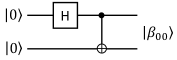
Figure 1. A quantum circuit for preparing the Bell state.

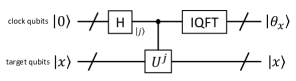
Figure 2. The quantum circuit for QPE algorithm.

$\bullet$ Measurement.  In quantum devices, qubit information can only be obtained through measurement. Measuring a quantum system yields a classical value with a probability corresponding to the amplitude. The state of the quantum system then collapses into a basis state according to the obtained value. For example, when measuring a qubit in state $a\left|0\right>+b\left|1\right>$, the result 0 is obtained with probability $|a|^{2}$, and the state collapses into $\left|0\right>$; the result 1 is obtained with probability $|b|^{2}$, and the state collapses into $\left|1\right>$. This property introduces uncertainty and impacts the testing of quantum programs.

$\bullet$ Quantum Operation.  A series of quantum gates can be represented as a unitary transform. However, measurement operations can disrupt the unitarity of the system. In quantum computing, a quantum operation is a mathematical model which is used to describe the general evolution, including both quantum gates and measurements, of a quantum system (nielsen2002quantum, ). Given an input density operator $\rho$ (a $d\times d$ matrix), the quantum operation $\mathcal{E}$ transforms it to $\mathcal{E}(\rho)$. This transformation can be represented by the operator-sum representation (nielsen2002quantum, ), which is given by $\mathcal{E}(\rho)=\sum_{i}E_{i}\rho E_{i}^{\dagger}$, where $E_{i}$ is a $d\times d$ matrix. If $\sum_{i}E_{i}^{\dagger}E_{i}=I$, then $\mathcal{E}$ is called a trace-preserving quantum operation.

3.2. Quantum Algorithms

Quantum algorithms leverage the principles of quantum mechanics to tackle computational problems. In this section, we present an overview of seven algorithms that will be further explored in subsequent sections. Here, we provide a brief introduction, while the comprehensive details of each algorithm can be found in (nielsen2002quantum, ) and (harrow2009quantum, ).

$\bullet$ Grover Search (GS).  Grover’s search algorithm (GS) (grover1996fast, ) has been proven to outperform classical search algorithms. The circuit diagram of GS is shown in Figure 3. It comprises approximately $O(\sqrt{N})$ iterations denoted as $G$, where $N=2^{n}$ represents the maximum number of elements. Each iteration includes an oracle call and a phase flip subroutine. Remarkably, GS enables the search of a database with $N$ elements using only $O(\sqrt{N})$ oracle queries (10.5555/870802, ).

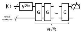
(a) The overall quantum circuit for Grover search.

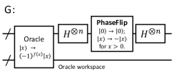
(b) The quantum circuit for the Grover iteration G.

Figure 3. The quantum circuits for Grover search algorithm.

$\bullet$ Quantum Fourier Transform (QFT).  Consider the following transform:

$$\left|j\right>\rightarrow\frac{1}{\sqrt{2^{n}}}\sum_{k=0}^{2^{n}-1}e^{2\pi ijk/2^{n}}\left|k\right>$$

This transform encodes the Fourier coefficients in the amplitudes of the quantum state, known as the Quantum Fourier Transform (QFT). This algorithm requires only $O(n^{2})$ steps for $n$-qubit inputs, compared to the classical fast Fourier transform (FFT), which requires $O(n2^{n})$ steps. QFT also has an inverse transform, denoted as IQFT.

$\bullet$ Quantum Phase Estimation (QPE).  QPE is a typical application of QFT to obtain the eigenvalue of a given eigenvector of a target unitary operation. Let $U$ be a unitary operation, and suppose it has an eigenvector $\left|x\right>$ with eigenvalue $e^{2\pi i\theta_{x}}$ (Note that the length of the eigenvalue of any unitary matrix is 1). The quantum phase estimation (QPE) algorithm estimates $\theta_{x}$ and encodes its binary representation in a multi-qubit quantum state $\left|\theta_{x}\right>$. The overall circuit for the QPE algorithm, as shown in Figure 2, consists of two groups of qubits: the target qubits and the clock qubits. The target qubits are initialized in the state $\left|x\right>$, and the clock qubits are initialized in an all-zero state. The binary representation of $\theta_{x}$ is then output on the clock qubits.

$\bullet$ Quantum Order Finding (QOF).  The order finding algorithm takes two positive integers input, $x$, and $N$, and computes the order of $x$ modulo $N$, i.e., the minimum value of $r$ satisfying $x^{r}\equiv 1(mod\hskip 2.84526ptN)$. QOF is a quantum algorithm that achieves order finding with a time complexity of $O(L^{3})$, where $L$ represents the length of the binary representation of the input numbers. Currently, no classical order-finding algorithm with polynomial time complexity has been discovered for comparison. The key concept of QOF involves applying QPE on the modular-multiply transform:

$$U\left|y\right>=\left|xy\hskip 2.84526pt(mod\hskip 2.84526ptN)\right>$$

Subsequently, the result obtained from QPE undergoes a continued fraction expansion in order to determine the order.

$\bullet$ Shor’s Quantum Factoring (Shor).  An order-finding algorithm can be employed to factorize a positive integer. Shor’s Quantum Factoring algorithm (shor1999polynomial, ) is built upon QOF. Since QOF is exponentially faster than any known classical order-finding algorithm, it enables the discovery of non-trivial factors for composite numbers $N$ with a time complexity of $O((\log N)^{3})$. Consequently, Shor’s algorithm efficiently factors a given number. This algorithm holds significant importance as it has the potential to break certain cryptosystems, such as RSA, that rely on the complexity of large-number decomposition. Algorithm 1 outlines the process of finding a non-trivial factor for an input composite number $N$. In addition to the QOF subroutine, it involves procedures for testing whether $N$ is in the form of $a^{b}$ and finding the greatest common divisor (GCD).

Input: A composite number $N$.

Output: A non-trivial factor of $N$.

1 If $N$ is even, return 2;

2 Determine whether $N=a^{b}$ for integers $a\geq 1$ and $b\geq 2$, and if so return $a$;

3 Randomly choose $x$ in the range $1$ to $N-1$. If GCD$(x,N)>1$ then return GCD$(x,N)$;

4 Use QOF subroutine to find the order $r$ of $x$ modulo $N$;

If $r$ is even and $x^{r/2}\neq-1\mod N$, then compute GCD$(x^{r/2}-1,N)$ and GCD$(x^{r/2}+1,N)$. Test to see if one of these is a non-trivial factor, and return the factor if so. Otherwise, the algorithm fails.

Algorithm 1 Quantum_Factoring

$\bullet$ Quantum Hamiltonian Simulation (QHSim).  The evolution of a closed quantum system satisfies the following equation:

$$\left|\psi(t)\right>=e^{-iHt}\left|\psi(0)\right>$$

In this equation, $H$ represents the Hamiltonian of the system, $\left|\psi(0)\right>$ is the state of the system at time $0$, and $\left|\psi(t)\right>$ is the state of the system at time $t$. QHSim is a technique that enables the implementation of the unitary transformation $e^{-iHt}$ for a given Hamiltonian $H$ and time $t$.

$\bullet$ Harrow-Hassidim-Floyd Algorithm (HHL).  The HHL algorithm (harrow2009quantum, ), introduced by Harrow, Hassidim, and Lloyd, offers a quantum approach to solving linear systems of equations. This algorithm tackles the problem of determining the unknown vector $x$ in the equation $Ax=b$, where $A$ represents a coefficient matrix of full rank, and $b$ is a constant vector. Figure 4 illustrates the core circuit of the algorithm. It encodes the matrix $A$ into a Hamiltonian and utilizes QHSim to implement the gate $e^{iAt}$ and its inverse $e^{-iAt}$. The vector $b$ is encoded into the amplitude of the quantum state $\left|b\right>$. The algorithm incorporates a phase estimation step, QPE, for the gate $e^{iAt}$ and the state $\left|b\right>$. The resulting state $\left|\lambda\right>$ is then used to apply a controlled rotation gate, CRot, which is a critical operation within the algorithm. Subsequently, an inverse phase estimation is applied for uncomputation, followed by the measurement of the ancilla qubit. The circuit is repeated until the measurement result is 1; at this point, the final output corresponds to the solution state $\left|x\right>$. Ideally, leveraging $n$ qubits, the HHL algorithm has the potential to solve an exponential number of linear systems using polynomial resources, thanks to the $2^{n}$ amplitudes provided by $n$ qubits.

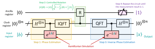
Figure 4. The core quantum circuit of the HHL algorithm.

4. The Properties of Multi-Subroutine Quantum Programs

To develop testing processes for multi-subroutine quantum programs, it is crucial to understand the important properties in these programs that impact testing designs. This section addresses the following research question (RQ):

• RQ1: What are the critical properties of multi-subroutine quantum programs, and how do they impact testing?

To address RQ1, we need to identify critical properties that influence testing designs for multi-subroutine quantum programs. Notably, these properties have not been adequately considered in current testing methods for quantum programs. We can identify these properties through two surveys: (1) investigating the supported features of quantum programming languages and (2) examining existing quantum software projects. Next, we will discuss each of these two surveys in detail.

4.1. Surveys on Quantum Programming Languages and Quantum Software Projects

4.1.1. Survey on Quantum Programming Languages

Several quantum programming languages have become available in recent years, such as Scaffold (abhari2012scaffold, ), Cirq (cirq2018google, ), Quipper (green2013introduction, ), Qiskit (gadi_aleksandrowicz_2019_2562111, ), Q# (svore2018q, ), Silq (bichsel2020silq, ), and isQ (Guo2022isQ, ). These languages differ in their design and capabilities. Some, such as the Python-based Qiskit, extend classical programming languages, while others, like Q#, are independent of their classical counterparts. Some languages, such as Cirq, are lower-level and suited for describing quantum circuits, while others, such as Q#, are higher-level and capable of implementing complex function calls. Additionally, almost all quantum programming languages provide simulators that enable programmers to run quantum programs on a classical computer. Some programming languages even offer interfaces to real quantum hardware. For example, Qiskit has an interface to IBM’s quantum hardware.

We first conduct a survey on these quantum programming languages. Table 1 presents a brief summary of the features of seven quantum programming languages that offer quantum development kits (QDKs) for building executable quantum programs. In this paper, we aim to test quantum programs with multiple subroutines and therefore focus on language features related to program structure and organization. We use the Q# language as our primary language of choice since it supports a broad range of quantum program structures and has extensive user documentation. Although our methods primarily utilize Q#, they are adaptable to other quantum programming languages as well; we will also explore testing strategies when the chosen language lacks some of the features described in this paper.

Table 1. The features of seven quantum programming languages

Feature Type		Scaffold	Cirq	Quipper	Qiskit	Q#	Silq	isQ
Language	Host language1	C	Py	Ha	Py	SA	SA	SA
Program Structure	Type system	✓		✓		✓	✓	✓
	Classical control flow	H	H	H	H	✓	✓	✓
	Classical-quantum mix	H	H	H	H	✓	✓	✓
Subroutine	Subroutine calling	H	H	H	H	✓	✓	✓
	Subroutine as parameters			H	H	✓	✓
Quantum- related	Qubit array	✓	✓	✓	✓	✓	✓	✓
	Endian modes of qubits					✓
	Auto-generate gate variants					✓	✓	✓
	Gate definition by matrix/list	✓	✓		✓			✓

• ’C’/’Py’/’Ha’ refers to C/Python/Haskell as the host language, while ’SA’ indicates that the quantum programming language is a standalone language.

• ’✓’ signifies that the quantum programming language provides support for the feature, ’H’ indicates that the feature is supported by the host language, and a blank space means that the quantum programming language does not support the feature.

4.1.2. Survey on Quantum Software Projects

We next conduct a survey on examining current quantum software projects on GitHub. However, we found very few open-source projects that included multi-subroutine quantum programs besides the built-in libraries within quantum software stacks. To overcome this limitation, we selected two quantum programming languages, Q# and Qiskit, and investigated the libraries they provide. We focus on libraries relevant to practical applications and algorithms of quantum computing rather than underlying support. For Q#, we selected three libraries Numerical, Chemistry, and MachineLearning, while for Qiskit, we selected Aqua Chemistry, Finance, and MachineLearning. Table 2 shows the 16 properties we identified, divided into four groups, and the number of subroutines that satisfied each property in each project. We will discuss the details of each property in the rest of this section. From the survey process and the results shown in Table 2, several key observations can be made:

• Practical quantum algorithms often incorporate classical subroutines for necessary pre- and post-processing steps. This hybrid approach leverages the strengths of both classical and quantum computation.

• Quantum algorithms implemented in the application layer frequently operate on variable qubit sizes, adapting to the specific requirements of the problem.

• Many subroutines within quantum algorithms rely on other subroutines to accomplish their intended tasks, indicating a modular and interconnected nature of quantum program design.

• Notably, there exist distinctions in the overall program structures between Q# and Qiskit, attributed to the specific features of these two programming languages. Qiskit, being hosted by Python, often employs object-oriented programming techniques. On the other hand, Q# exhibits characteristics more aligned with a functional programming language.

These findings provide valuable insights into the characteristics and design considerations of quantum software development.

Table 2. The number of subroutines in six quantum projects in Q# and Qiskit which meet specific properties

		Q#			Qiskit
		Numerics	Chemistry	Machine- Learning	Aqua Chemistry	Finance	Machine- Learning
General	1.1 Total count	98	131	54	557	86	421
	1.2 Classical	9	46	27	537	79	414
	1.3 Fixed qubits size	0	0	0	0	0	0
	1.4 Variable qubits size	89	84	27	10	7	7
Program structure	2.1 Linear1	54	66	29	343	49	257
	2.2 Has ”if-then” block	16	46	11	183	22	150
	2.3 Has ”for” loop	15	37	25	127	14	46
	2.4 Has ”try” block	0	0	0	6	9	16
	2.5 Has ”while” loop2	0	1	0	5	0	2
	2.6 Has ”within-apply”	17	0	0	0	0	0
Subroutine calling	3.1 No calling	0	13	8	145	37	149
	3.2 Has calling	98	118	46	411	39	269
	3.3 As input parameter	0	25	10	7	0	4
Variants	4.1 Original	36	71	44	557	85	421
	4.2 Inverse	44	40	13	0	1	0
	4.3 Controlled	42	39	12	0	0	0

• ”Linear” means the subroutine is the sequential execution of statements without any special structure.

• Including repeat-until-success structure.

4.2. The Structure of Quantum Programs

4.2.1. Quantum Circuits and Quantum Programs

The quantum circuit model, which represents a linear sequence of quantum gates applied from left to right, is commonly used to describe quantum algorithms, as shown in Figure 2 for the QPE algorithm. Current research on quantum testing mainly focuses on the circuit model (wang2018quanfuzz, ; wang2021application, ; wang2021generating, ; wang2022mutation, ; abreu2022metamorphic, ). However, to describe algorithms that include gates controlled by classical values from measurements, an improvement to the circuit model, called dynamic circuit model (Hua2023CaQR, ; Corcoles2021DynamicCirc, ), has been proposed. Figure 5 shows a typical dynamic circuit implementing quantum teleportation, which contains two gates controlled by measurement results. Listing 1 shows the Q# code implementation of this circuit, where gates controlled by measurement results are implemented using if statements (lines $7\sim 10$). However, quantum circuits are not always equivalent to quantum programs, as the circuit model is hard to describe while loops and quantum-classical-hybrid algorithms.

Figure 5. The quantum circuit for quantum teleportation.

Listing 1: The Q# code for teleportation program

⬇

1operation TeleportQubit(qsrc : Qubit, qanc : Qubit, qdest : Qubit) : Unit {

2 H(qanc);

3 CNOT(qanc, qdest);

4 CNOT(qsrc, qanc);

5 H(qsrc);

6 let m2 = M(qanc);

7 if (m2 == One) { X(qdest); }

8 let m1 = M(qsrc);

9 if (m1 == One) { Z(qdest); }

10}

Practical quantum algorithms often consist of both classical and quantum parts. In some cases, the algorithm’s input contains both classical and quantum variables, such as parameterized quantum circuit (PQC) (marcello2019PQC, ), widely used in quantum machine learning. A PQC can be denoted as $U_{\phi(\vec{x})}$, where vector $\vec{x}$ represents the classical data and $\phi$ is the encoding function. Different values of $\vec{x}$ result in different circuits, and thus $\vec{x}$ is the classical input of the PQC. In other cases, the entire program consists of both classical and quantum subroutines, as seen in quantum factoring (Algorithm 1), where the unique quantum subroutine is quantum order finding (QOF) and the other subroutines are classical.

Unlike a fixed-size quantum circuit, a general quantum program corresponds to a family of quantum circuits rather than a specific circuit. For example, the quantum Fourier transform (QFT) program (Figure 6) corresponds to different circuits based on the number $n$ of qubits used. It is similar to its classical counterpart, the Boolean circuit model (arora2009computational, ), an essential computational model in computational complexity theory. Classical algorithms typically correspond to a uniform family of Boolean circuits rather than just one circuit.

This paper focuses on testing quantum programs containing both quantum and classical code rather than just quantum circuits.

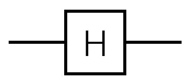
(a) $n=1$

(b) $n=2$

(c) $n=3$

(d) $n=4$

Figure 6. The corresponding circuits of QFT program with $n=$ 1, 2, 3, 4 respectively ($n$ is the number of qubits).

4.2.2. Control flows in Quantum Programs

Classical control flows in quantum programs are also crucial for programming and designing practical quantum algorithms. Similar to classical programs, quantum programs frequently utilize if statements, for/while loops, and other control flow structures to achieve their desired outcomes. For instance, Listing 1 employs if statements to implement gates controlled by measurement results. Moreover, Listing 3 presents an implementation of the QFT program using for loops to iterate over qubits of varying sizes.

Quantum programs also employ while loops, which have a loop condition controlled by a variable instead of an iteration index. In quantum programming, the condition variable may depend on quantum measurement results. For example, the repeat-until-success (RUS) structure is often used in quantum programming. This structure relies on a success condition associated with measurement results. The loop continues to iterate until the success condition is satisfied. Listing 2 illustrates the implementation of a quantum program generating random integers 0, 1, and 2 with equal probability using a RUS structure.

Additionally, some quantum programs incorporate classical and quantum computing into one subroutine, which is referred to as a quantum-classical mixed (C-Q mixed) program. For example, QFT (Listing 3) contains a subroutine CRk, which takes classical expressions (line 3) to calculate an intermediate parameter ”theta.” This combination of classical and quantum computing is often required in developing practical quantum algorithms, such as Grover search and quantum machine learning.

Listing 2: The Q# code for generating random numbers 0, 1, and 2

⬇

1operation Random_0to2() : Int {

2 use qs = Qubit[2];

3 mutable m = 0;

4 repeat {

5 ResetAll(qs);

6 H(qs[0]);

7 H(qs[1]); //Generate uniform superposition state

8 set m = ResultArrayAsInt(MultiM(qs));

9 } until (m < 3); //Success condition

10 ResetAll(qs);

11 return m;

12}

4.3. Subroutines

4.3.1. The Organization of Subroutines

In software development, programmers often use ”structured programming,” (dahl1972structured, ) where a large program is decomposed into several subroutines and organized by function calls. This programming paradigm improves the readability and testability of code and allows the reuse of commonly used subroutines. As shown in Listing 3, CRk and Reverse are two subroutines called by the upper-level program QFT.

Besides direct calls, another way to organize subroutines is to take the subroutine as an input parameter. An example is Grover Search (grover1996fast, ), which needs an oracle to identify a solution and uses the subroutine as a black box. The oracle can be implemented as an input subroutine. Listing 4 shows another example QPE, which requires the target quantum operation as an input parameter (Upower in lines 1 and 8).

Listing 3: The Q# code for QFT program

⬇

1operation CRk(qctrl: Qubit, k: Int, qtarget: Qubit) : Unit is Adj {

2 body(...) {

3 let theta = 2.0 * Math.PI() / Convert.IntAsDouble(2 ^ k);

4 Controlled R1([qctrl], (theta, qtarget));

5 }

6 adjoint auto;

7}

8

9operation Reverse(qs : Qubit[]) : Unit is Adj {

10 body(...) {

11 let n = Length(qs);

12 for i in 0 .. n / 2 - 1

13 { SWAP(qs[i], qs[n - i - 1]); }

14 }

15 adjoint auto;

16}

17

18operation QFT(qs : Qubit[]) : Unit is Adj {

19 body(...) {

20 let n = Length(qs);

21 for i in 0 .. n - 2 {

22 H(qs[i]);

23 for j in i + 1 .. n - 1 {

24 let k = j - i + 1;

25 CRk(qs[j], k, qs[i]); // Call "CRk"

26 }

27 }

28 H(qs[n - 1]);

29 Reverse(qs); // Call "Reverse"

30 }

31 adjoint auto;

32}

Listing 4: The Q# code for QPE program

⬇

1operation QPE(Upower : (Int, Qubit[]) => Unit is Adj + Ctl,

2 qsclock : Qubit[], qstarget : Qubit[]) : Unit is Adj {

3 body (...) { //Original operation

4 let n = Length(qsclock);

5 MultiH(qsclock);

6 for i in 0 .. n - 1 {

7 Controlled Upower([qsclock[n - i - 1]], (2 ^ i, qstarget));

8 }

9 Adjoint QFT(qsclock);

10 }

11 adjoint auto; //Generate adjoint version of QPE by Q#.

12}

4.3.2. Three Variants of a Subroutine

In quantum programs, there are three important variations of subroutines: the inverse, controlled, and power variants, which can also be combined. Formally, for a unitary operation $U$, its variations include the inverse ($U^{-1}$), controlled (Controlled-$U$), and power ($U^{n}$) variants. These variants are crucial for quantum software development. For example, in Listing 4, the QPE program calls the Adjoint QFT (line 9), the inverse of QFT, and the Controlled Upower (line 7), which is the controlled version of Upower. It is important to note that these variants represent distinct subroutines compared to their original programs.

Some high-level quantum programming languages, such as Q# (svore2018q, ) and isQ (Guo2022isQ, ), support the generation and management of these three variants. As an example, Listing 5 gives an implementation of $H^{n}$, the power of the $H$ gate, which uses these variants. The power $n$ is implemented as an extra Int parameter power. Based on the result of $H^{2}=I$, we can obtain that $H^{n}=H$ if $n$ is odd; otherwise, $H=I$ (line 4). The inverse, controlled, and inverse-and-controlled variants can be generated automatically by Q# (lines 6-8), which uses the keyword “adjoint” to represent inverse operation. However, this mechanism of automatically generating variants via programming languages is not always available. Sometimes we still need to write variants manually, which may lead to bugs. Therefore, it is necessary to propose specific techniques to test variants. We will discuss this issue in Section 6.4.3.

Listing 5: The implementation of the power variant of the H gate. The adjoint, controlled, and adjoint controlled versions are generated by Q# automatically.

⬇

1operation Hpower(power : Int, q : Qubit) : Unit is Adj + Ctl {

2 body (...) {

3 //If pow is odd, apply H, otherwise I

4 if (power % 2 == 1) { H(q); }

5 }

6 adjoint auto;

7 controlled auto;

8 adjoint controlled auto;

9}

4.3.3. Within-Apply Structure

The within-apply (WA) structure is a common structure in quantum programs and is supported in the Q# language with syntactic sugar. Formally, this structure can be represented as

$U^{-1}VU$

Here, the execution order is from right to left: the subroutine $U$ creates an environment, and the subroutine $V$ operates on that environment. Once $V$ has been executed, the environment must be recovered to its original state, which is accomplished by applying $U^{-1}$. Figure 7 provides an example of a WA structure, which shows the decomposition of a Controlled-X gate controlled by the binary string ”1001”. The target gate is applied by default when the controlling qubit is 1; however, if we want it to be controlled by 0, an X gate must be added before the default controlling gate. In addition, we must also recover the controlling qubits to their original state, which is achieved by applying an $\texttt{X}^{-1}$ (= X) gate after the default controlling gate. This WA structure can be implemented in Q# using the code shown in Listing 6, which utilizes the ”within $U$ apply $V$” statement to implement $U^{-1}VU$, with $U^{-1}$ being calculated automatically. Another example is the HHL program, as shown in Figure 4. In this case, $U$ is QPE, and $V$ is the controlled rotation CRot.

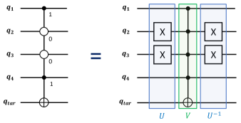
Figure 7. The decomposition of the Controlled-X gate is controlled by 1001. On the left is the note in the quantum circuit, where 0-controlling qubits are with hollow circles. It can be decomposed to the right with a standard controlled-X gate between the two X gates on the 0-controlling qubits.

Listing 6: The corresponding Q# code of Figure 7.

⬇

1operation C_nC_nC_C_X(q1 : Qubit, q2 : Qubit, q3 : Qubit,

2 q4 : Qubit, qtar : Qubit) : Unit is Adj + Ctl {

3 body (...) {

4 within {

5 X(q2);

6 X(q3);

7 }

8 apply {

9 Controlled X([q1, q2, q3, q4], qtar);

10 }

11 }

12 adjoint auto;

13 controlled auto;

14 adjoint controlled auto;

15}

4.4. Input and Output

4.4.1. Input, output, and IO types of quantum programs

Testing design is typically based on the input and output of programs under test. Previous research (ali2021assessing, ; wang2021generating, ; wang2021application, ) has defined the input and output of a quantum program as a subset of all used qubits. However, this definition only considers qubit variables and neglects other possible types of input and output variables. In practice, many quantum subroutines contain other types of input or output variables, such as classical parameters or parameters of subroutines. For example, Listing 3 shows that subroutine CRk contains a classical integer input parameter k, while Listing 4 requires Upower, an input of another subroutine, to be estimated. Therefore, it is valuable to classify quantum programs based on their input and output. Since quantum variables will influence the testing design, based on whether their input or output contains quantum variables, we can classify quantum subroutines into four IO types as follows.

• Type 1 - Classical: The subroutine has no input and output quantum variables.

• Type 2 - Generate-Quantum: The subroutine has input quantum variables but no output quantum variables.

• Type 3 - Detect-Quantum: The subroutine has output quantum variables but no input quantum variables.

• Type 4 - Transform: The subroutine has both input and output quantum variables.

Here, the term ”quantum variable” refers not only to qubits or qubit arrays but also subroutines that take qubits or qubit arrays as inputs or outputs. For example, in Listing 4, the qubit arrays qsclock and qstarget in line 2 are quantum input variables. Additionally, the Upower subroutine in line 1, which takes a qubit array as input, is also a quantum input variable. Figure 8 illustrates the data flow for the four IO types, showing the dependencies of classical input (c-in), quantum input (q-in), classical output (c-out), and quantum output (q-out).

(a) Classical

(b) Generate-Quantum

(c) Detect-Quantum

(d) Transform

Figure 8. The data flow of four types of quantum subroutines.

4.4.2. Logical meaning of quantum variables

It is also crucial to consider the logical meaning of quantum variables. For instance, consider the quantum adder program QAdd:

(1) $$\texttt{QAdd}:\left|x\right>\left|y\right>\rightarrow\left|x\right>\left|x+y\right>$$

In QAdd, the contents of quantum registers represent integers and add the first integer to the second. The quantum registers of $\left|x\right>$ and $\left|y\right>$ logically correspond to two sets of qubits. Therefore, the program’s input should contain two quantum variables $\left|x\right>$ and $\left|y\right>$ instead of taking all qubits as one input variable. Correctly identifying the inputs and outputs of all program subroutines is a critical prerequisite for successfully finishing the testing task of a target program under test. We provide a more detailed discussion in Section 6.1.

4.4.3. Endian modes

In classical computing, the computer architecture guarantees the endian mode of an integer, and programmers do not need to consider it while dealing with integers at the word level. However, current quantum computing still operates on the qubit level and requires programmers to consider the order (endian mode) of the qubits when programming quantum variables containing more than one qubit, such as quantum integers. Mismatched endian modes of two quantum subroutines can lead to errors. Figure 9 illustrates four possible qubit orders for the QFT program - input with big-endian (BI) or little-endian (LI) and output with big-endian (BO) or little-endian (LO). The QFT implementation in Listing 3 is in BIBO mode, the typical implementation. However, if the calling of Reverse (line 29) is missed, it will result in BILO mode.

To manage the endian of qubit arrays, some programming languages, such as Q#, provide a preliminary mechanism. In the Q# standard library, types Bigendian and Littleendian are two different encapsulations of the raw qubit array (Qubit[]). The QFT() function in the standard library requires a Bigendian parameter and is implemented in BIBO mode, while the function QFTLE() takes a Littleendian parameter and is implemented in LILO mode. Proper management of the endian of qubit arrays can help programmers avoid errors and ensure the correct implementation of quantum programs.

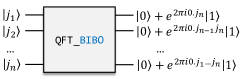
(a) Big-endian input and big-endian output

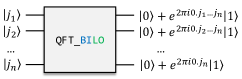
(b) Big-endian input and little-endian output

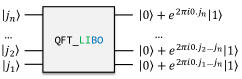
(c) Little-endian input and big-endian output

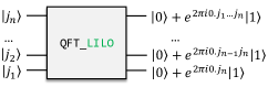
(d) Little-endian input and little-endian output

Figure 9. Four possible IO endian modes for QFT program. Input integer $j=j_{1}j_{2}\cdots j_{n}$, i.e., $j_{1}$ is the highest bit of $j$. The index of qubit increases from top to bottom in each subroutine.

4.5. Program Specification

Program specification gives the expected behavior of the program and is the foundation of testing execution. The purpose of testing is to check whether a program converts the given input into a specific output according to the program specification.

4.5.1. Probability-based program specification

Previous research (wang2021generating, ; ali2021assessing, ; wang2021application, ) defined the program specification as the expected probability distribution of the output values under given input values. It is so-called probability-based program specification. For example, the program in Listing 2 has no input variable, and we expect the output to be a uniform distribution on $\{0,1,2\}$. So the program specification can be written as follows:

Input: none.   Output: (0 with $p_{0}=\frac{1}{3}$), (1 with $p_{1}=\frac{1}{3}$), (2 with $p_{2}=\frac{1}{3}$)

4.5.2. Formula-based program specification

Probability-based program specification implies that we must have a measurement at the end of each subroutine to convert quantum states into probability distributions. This restriction is not suitable for testing multi-subroutine programs. In a multi-subroutine program, its subroutine often transforms a quantum state into another state without measurement at its end. It is, therefore, better to consider the specification of quantum states rather than a probability distribution. Generally, for some given inputs, the program specification gives the expected output for each input. This relationship can be represented as a formula in most cases, and we call it formula-based program specification. For example, Formula (1) is an example of the description of QAdd program, and QFT program has the following formula description:

(2) $$\texttt{QFT}:\left|j\right>\rightarrow\frac{1}{\sqrt{2^{n}}}\sum_{k=0}^{2^{n}-1}e^{2\pi ijk/2^{n}}\left|k\right>$$

where $\left|j\right>$ is a classical state with integer $j$. Formula (2) only gives the transform under classical state inputs. Fortunately, QFT is a unitary transform, so the expected output under general input can be deduced by linearity.

More precisely, the formula (2) can be rewritten in bitwise form, which is related to the endian mode. Suppose we adopt BIBO mode (Figure 9(a)), then

(3) $$\texttt{QFT\_BIBO}:\begin{array}[]{c}\left|j_{1}\right>\rightarrow\frac{1}{\sqrt{2}}(\left|0\right>+e^{2\pi i0.j_{n}}\left|1\right>)\\ \cdots\\ \left|j_{n}\right>\rightarrow\frac{1}{\sqrt{2}}(\left|0\right>+e^{2\pi i0.j_{1}j_{2}\ldots j_{n}}\left|1\right>)\end{array}$$

where $n$ is the length of $j$ and $j=j_{1}j_{2}\ldots j_{n}$. Formula (3) gives the output state on each qubit under the input $\left|j_{1}\right>\left|j_{2}\right>\ldots\left|j_{n}\right>$.

4.6. Quantum State Generation and Detection

Testing quantum programs rely heavily on the handling of quantum variables. However, generating and detecting quantum states have more significant challenges than their classical counterparts due to the properties of quantum states.

In classical computing, input parameters can easily be fed into a computer. A natural language description of the input, such as a block of text or a decimal number, can be converted into a binary string according to predetermined coding rules. This binary string is then converted into the internal state of a computer’s components (e.g., high and low voltages represent 1 and 0, respectively). However, quantum variables not only have classical states like binary strings, but they also have superposition states or mixed states. Some states that can be easily described in natural language may be difficult to prepare on quantum devices. For example, for general superposition states, the algorithm proposed by (Lov2002Creating, ) can be used to generate the superposition state $\sum_{i}\sqrt{p_{i}}\left|i\right>$ if we know the probability distribution $\{p_{i}\}$ of each amplitude. However, this algorithm can be computationally expensive if the target states do not have specific properties. In fact, it has been proven that preparing some quantum states requires exponential costs (knill1995approximation, ).

Once a quantum program has been executed with a given input, the next step is to compare the actual output with the expected output. While reading classical memory is relatively straightforward, quantum computing presents a challenge when it comes to comparing output containing quantum variables. Measurements must be made to extract information about these variables, but they may cause the state of the quantum variables to collapse and interfere with the program’s execution. Consequently, many classical testing methods that depend on intermediate variables cannot be directly applied to test quantum programs.

In the field of quantum information, various methods have been proposed to solve problems concerning quantum state detection, such as quantum distance estimation (Flammia2011FewPauli, ; Cerezo2020VariationalQF, ), quantum discrimination (Stephen2008Discrimination, ; zhang2006300discri_mixed, ; Zhang2007discri_puremix, ), quantum tomography (tomography1989, ; Chuang1996statetomo, ), and the Swap Test (buhrman2001quantum, ; ekert2002direct, ). Unfortunately, almost all methods require multiple copies of the target quantum state, and the results are not entirely accurate. This is particularly challenging in testing practice, as it often requires repeating the execution of the target program.

5. The Overall Testing Process

In this paper, we propose a systematic testing process for multi-subroutine quantum programs, which involves both unit testing and integration testing. We base our approach on the properties of these programs, which we discuss in Section 4. This section outlines the overall testing process, with detailed explanations provided in subsequent sections. Figure 10 depicts the three main steps in the testing process for multi-subroutine quantum programs: (1) structural analysis, (2) unit testing for each subroutine, and (3) integration testing.

Given a multi-subroutine quantum program, the first step is to analyze the structure of the whole program, identify its subroutines, and understand how they are organized. We use Q-UML (Perez-Delgado2020quantum, ), a quantum extension of the unified modeling language (UML), to specify the program’s structure. After that, we perform unit testing on each subroutine and integration testing on the entire program.

During unit testing, we start by analyzing the input and output of each subroutine to gather the necessary information for testing. We introduce a novel approach called IO marks to represent this information. We then break down the unit testing task into three subtasks: (1) quantum relation checking, (2) quantum structural testing, and (3) quantum behavioral testing. Depending on the testing requirements, a unit testing task may involve one or more subtasks. In Section 6, we will provide details on unit testing, along with novel testing principles and criteria for quantum programs.

After performing the unit testing of all subroutines, we proceed with integration testing of the entire program. In practice, testing tools are often used to support testing tasks. Section 7 will delve into the details of integration testing and the testing tool requirements for multi-subroutine quantum programs.

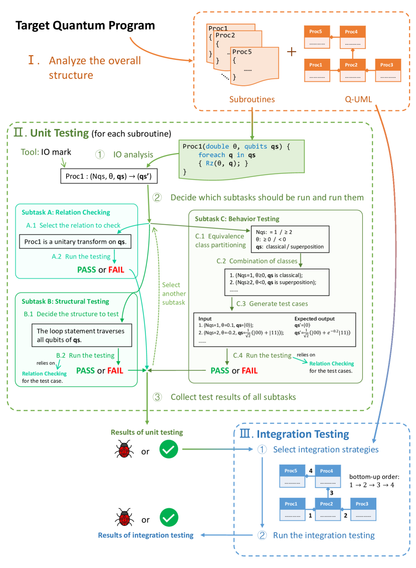
Figure 10. The overall process of testing quantum programs with multiple subroutines.

6. Unit Testing

In this section, we discuss the details of unit testing. We discuss the steps of IO analysis in Section 6.1. As depicted in Figure 10, a unit test consists of three subtasks, each performing one or more subtasks based on its specific testing requirements. We begin by examining some general test criteria in Section 6.2, followed by a detailed exploration of these subtasks from Section 6.3 to Section 6.6. Additionally, we discuss the generation and execution of each test case in Section 6.7.

6.1. IO Analysis

IO analysis involves identifying the input and output variables of a subroutine. As Section 4.4 mentions, this analysis is the foundation for unit testing. In order to streamline the test design process, it is important to focus on the minimal subset of variables relevant to the test design. Specifically, for a concrete subroutine, only the variables that users need to assign are considered inputs, while only the variables that users are interested in after execution are considered outputs. For example, in many quantum algorithms, some qubits should always be initialized with an all-zero state $\left|0\ldots 0\right>$. These qubits should not be regarded as input. Another typical case is a qubit array, such as qs in Listing 3 (line 18). Like an array of integers, a qubit array contains both length and data. Therefore, when identifying the input and output of a subroutine, a qubit array should be regarded as two variables: length and quantum state.

To represent the input and output of a quantum program, we introduce the IO mark, which can help developers design test cases. The general form of the IO mark is:

program : (input variables) $\rightarrow$ (output variables’)

We use underline to denote the input parameters of subroutine type and bold font to denote quantum variables. These two marks can be combined to represent subroutine type with quantum variables. The idea to represent quantum-related content in bold font comes from the Q-UML modeling language (Perez-Delgado2020quantum, ). We add an “apostrophe” (’) on each output variable to distinguish input and output. If a variable var is both input and output, we denote the input and output as the same name, i.e., var is the input, and var’ is the output. Sometimes, we need to specify the endian mode for multi-qubit quantum variables. In this case, we add the variables with ”BE” (big-endian) or ”LE” (little-endian) superscript, such as qvar^BE.

According to Section 4.4, quantum subroutines can be classified into four types, and different types of quantum programs have different testing strategies. Having the IO mark, we are able to know which type the target program is. Example 6.1 shows how to perform IO analysis and use IO marks.

Example 6.0.

IO analysis for QPE program.

The QPE program in Listing 4 has three parameters: Upower, qsclock, and qstarget, while the latter two are qubit-array types. On the input side, qsclock contains two variables: the length “Nclock” and the data “clock.” It is similar to qstarget, which contains two variables as well: the length “Ntarget” and the data “target.” On the output side, they should be denoted as “clock’” and “target’.” Upower is a parameter of quantum subroutine type and should be denoted as “Upower.” Figure 11 shows the structure, input, and output of the QPE program.

In the program, the quantum state clock is always initialized with an all-zero state, so it is not an input. In most applications of the QPE program, we do not care about the post-state target’, so it is not output. In Figure 11, the input variables are shown in green, while the output variable is shown in red. The endian mode of the target is not important, but that of the clock’ is important since the clock’ stores the binary representation of $\theta_{x}$. Subroutine Adjoint QFT is of BIBO endian mode, so the output state clock’ is of big-endian (BE) mode. The IO mark can be written as:

QPE : (Nclock, Ntarget, Upower, target) $\rightarrow$ (clock’^BE)

Obviously, QPE is a quantum program of transform type.

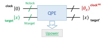
Figure 11. The diagram illustrates the input and output of the QPE program, with the input variables represented in green and the output variable denoted in red.

6.2. Generic Testing Principles and Criteria

After finishing the IO analysis of a subroutine, the next step is performing unit testing by executing some subtasks. Before that, we need to discuss the generic testing criteria which can guide our testing tasks.

A testing criterion is a set of rules used to help determine whether a program is adequately tested by a test suite and guides the testing design (ammann2016introduction, ). Some coverage criteria for quantum programs have been proposed, such as Quito (quantum input-output coverage) (ali2021assessing, ), suitable for small-scale and fixed-scale quantum programs. However, there is still a lack of testing criteria for multi-subroutine quantum programs in previous work. This section will propose some quantum-related testing criteria and principles according to the properties of quantum variables and quantum programs. We will narrate each criterion or principle and give the reason or theoretical basis for adopting it.

6.2.1. Basic testing principles

Quantum programs require special attention when selecting quantum inputs due to the distinct properties of quantum states compared to classical programs. As a result, we suggest the following principle for carefully considering the selection of quantum inputs:

Principle 1.

The basic principle of quantum input selection:

• (1) Selected input states should be representative;

• (2) Input quantum states should be easy to prepare;

• (3) Corresponding output quantum states should be also easy to check.

In Principle 1, (1) guarantees the validity of the test task, which is a similar requirement in testing classical programs. (2) and (3) are based on the fact that generating and checking general quantum states may require complex processes (see Section 4.6), which may easily lead to errors. In the following sections, we will discuss some representative input states that are valuable for detecting errors and are relatively easy to generate. We will also discuss some representative methods for checking output states.

6.2.2. Partition quantum input by state type

In a testing task, we need to select some appropriate inputs to run the target program. Equivalence class partitioning is an important testing method for classical programs (ammann2016introduction, ). The basic idea is to partition the input space into several ”equivalence classes” in a logical meaning, where all cases in one class have the same effect in finding bugs. Such an idea can also be applied to quantum program testing. For quantum programs with quantum input variables, we can consider the partition of quantum input variables. A natural, coarse-grained partitioning scheme is by type of quantum state. In general, there are three types of quantum states: classical, superposition, and mixed states (see Section 3.1). Thus, we can define a ”classical-superposition-hybrid partition.”

Principle 2.

Classical-superposition-mixed partition (CSMP).

For each input variable of each quantum state type, partition it into classical state input, superposition state input, and mixed state input.

However, since a mixed state can be considered as a probability distribution of several pure states (see Section 3.1) unless the program specification has special regulations about the mixed state, we can omit the coverage of the mixed state, which can be simplified to the ”classical superposition partition” as follows.

Principle 3.

Classical-superposition partition (CSP).

For each input variable of each quantum state type, partition it into classical state input and superposition state input.

Which principle should be used during testing is determined by whether the program specification has special regulations for mixed states. If it does, we can use CSMP. Otherwise, CSP is enough.

Note that whether using CSP or CSMP, both classical and superposition states should be covered. There are two reasons for this. First, the program specification often gives the expected output states of the program under a specific input state, and the given input states are usually classical (such as formula (2) in Section 4.5), so covering classical states is to check the specification directly. Second, superposition is the essential difference between classical and quantum variables, and testing classical input alone cannot ensure the program behavior in superposition input. We will discuss the necessity of covering superposition states in Section 8, where the result will be shown in Section 8.4.

The CSP and CSMP principles mentioned above are coarse-grained and represent minimal partitioning requirements. However, for a specific quantum program, a more fine-grained partitioning based on its logical meaning is necessary. In Section 6.6.1, we will further discuss equivalent partitioning.

6.2.3. Two testing criteria for quantum input selection

The selection of a specific input quantum state usually depends on the properties of the target program or the program specification. However, the following two selection criteria are applicable to general quantum programs and satisfy the CSP principle:

Criterion 1.

Single-and-two-value selection criterion (STV)

Select the quantum input states in the following three forms:

• 1. $\left|x\right>$: a classical state of single integer value $x$;

• 2. $\frac{1}{\sqrt{2}}(\left|x\right>+\left|y\right>)$: a superposition state of two values $x$ and $y$;

• 3. $\frac{1}{\sqrt{2}}(\left|x\right>+i\left|y\right>)$: a superposition state of two values $x$ and $y$, and the value of $y$ has an additional relative phase $i$, where $i^{2}=-1$.

Criterion 2.

Pauli selection criterion (PAULI)

Select the quantum input states from the $n$-qubit Pauli states:

(4) $$\{\left|0\right>,\left|1\right>,\left|+\right>,\left|-\right>,\left|+_{i}\right>,\left|-_{i}\right>\}^{\otimes n}$$

where $\left|+\right>=\frac{1}{\sqrt{2}}(\left|0\right>+\left|1\right>)$, $\left|-\right>=\frac{1}{\sqrt{2}}(\left|0\right>-\left|1\right>)$, $\left|+_{i}\right>=\frac{1}{\sqrt{2}}(\left|0\right>+i\left|1\right>)$, and $\left|-_{i}\right>=\frac{1}{\sqrt{2}}(\left|0\right>-i\left|1\right>)$, i.e., the eigenvectors of all $n$-qubit Pauli operators.

Appendix A shows the generation of quantum states based on the STV and PAULI criteria. In the following, we will discuss the rationality of using these criteria and their applicability.

$\bullet$ Theoretical Basis of STV Criterion.  A quantum program usually transforms the quantum input state into another state. An important fact is that a quantum program with if statements and while-loop statements, where the if and while-loop conditions can contain the result of measuring qubits, can be represented by a quantum operation (ying2016foundationQP, ). So we can model the behavior of a quantum program as a quantum operation, which transforms the quantum input density matrix space into the quantum output density matrix space (classical variables can be regarded as a restricted case of quantum variables). Interestingly, the quantum operation is a linear map on the input density matrix space, so its behavior depends on the behavior of a group of bases. For an $n$-qubit quantum system, the density matrix is of $2^{n}\times 2^{n}$, and thus, the dimension of the density matrix space is $4^{n}$.

Obviously, a group of bases is $\{\left|x\right>\left<y\right|\}$, where $x,y=0,1,\dots,2^{n}-1$, i.e., the matrix element is 1 on the location ($x,y$) and 0 on other locations. However, if $x\neq y$, $\left|x\right>\left<y\right|$ is not a legal quantum state because $tr(\left|x\right>\left<y\right|)=0\neq 1$. Fortunately, consider the following two states:

$$\left|+_{xy}\right>=\frac{1}{\sqrt{2}}(\left|x\right>+\left|y\right>),\qquad\left|-_{xy}\right>=\frac{1}{\sqrt{2}}(\left|x\right>+i\left|y\right>)$$

where $i^{2}=-1$. Then $\left|x\right>\left<y\right|$ can be decomposed into the linear combination of four pure states:

$$\left|x\right>\left<y\right|=\left|+_{xy}\right>\left<+_{xy}\right|+i\left|-_{xy}\right>\left<-_{xy}\right|-\frac{1+i}{2}\left|x\right>\left<x\right|-\frac{1+i}{2}\left|y\right>\left<y\right|$$

So for all $x,y=0,1,\dots,2^{n}-1$ and $x\neq y$, states with form $\left|x\right>$, $\left|+_{xy}\right>$, and $\left|-_{xy}\right>$ also constitute a group of bases. They are not orthonormal bases, but all elements are legal pure states, and thus they can be used as input states. They are the selected states in the STV criterion.

$\bullet$ Theoretical Basis of PAULI Criterion.  Another typical group of bases for density matrix space are all $n$-qubit Pauli matrices, i.e., the tensor product single-qubit Pauli matrices: $\sigma_{\vec{v}}=\sigma_{v_{1}}\otimes\sigma_{v_{2}}\otimes\cdots\otimes\sigma_{v_{n}}$, where $v_{i}\in\{0,1,2,3\}$, $\vec{v}=(v_{1},\dots,v_{n})$, and single-qubit Pauli matrices are

(5) $$\sigma_{0}=\left[\begin{array}[]{cc}1&0\\ 0&1\end{array}\right],\sigma_{1}=\left[\begin{array}[]{cc}0&1\\ 1&0\end{array}\right],\sigma_{2}=\left[\begin{array}[]{cc}0&-i\\ i&0\end{array}\right],\sigma_{3}=\left[\begin{array}[]{cc}1&0\\ 0&-1\end{array}\right]$$

However, $\sigma_{\vec{v}}$ is also not a legal quantum state, but we can decompose it into the sum of its eigenstates $\sigma_{\vec{v}}=\sum_{i}{\lambda_{i}\left|\psi_{i}\right>\left<\psi_{i}\right|}$, where $\lambda_{i}$ is the $i$-th eigenvalue of $\sigma_{\vec{v}}$ and $\left|\psi_{i}\right>$ is the corresponding eigenstate. $\left|\psi_{i}\right>$ is the tensor product of single-qubit Pauli eigenstate:

(6) $$\left|\psi_{i}\right>\in\{\left|0\right>,\left|1\right>,\left|+\right>,\left|-\right>,\left|+_{i}\right>,\left|-_{i}\right>\}^{\otimes n}$$

Actually, the freedom degree of $n$-qubit density operators is $4^{n}$, which means some Pauli eigenstates are not independent. Fortunately, it does not matter because, in a testing task, we often sample only a small subset of Pauli eigenstates.

$\bullet$ Applicability.  STV and PAULI are particularly useful for generating random input because they have completeness assurance. Both STV and PAULI criteria have their own characteristics and strength. Quantum input states from STV are controlled by two integer numbers, $x$ and $y$, so the STV criterion is useful in testing numerical quantum programs. The advantage of the PAULI criterion is that the quantum input states can be generated using only single-qubit gates, so it is useful on operation-constrained quantum devices (e.g., devices that do not support remote CNOT operation).

6.2.4. Superposition-Cover-All-Qubit Criterion

Since superposition input states are able to expose some bugs, which can occur at any qubit, it is necessary to require that superposition states exist at every qubit. In the following, we introduce a novel criterion: superposition-cover-all-qubit criterion (SCAQ).

Criterion 3.

Superposition-cover-all-qubit criterion (SCAQ)

Selecting a set of input states that meet the following requirement: ensuring that for each qubit in all quantum input variables, there must exist at least one state within the entire input set that exhibits superposition on that specific qubit.

The following example presents two sets of inputs, one satisfying SCAQ and another not.

Example 6.0.

The following input set satisfies SCAQ:

$$\{\frac{1}{\sqrt{2}}(\left|000\right>+\left|100\right>),\frac{1}{\sqrt{2}}(\left|000\right>+\left|010\right>),\frac{1}{\sqrt{2}}(\left|000\right>+\left|001\right>)\}$$

The superposition of the 1st qubit occurs in state $\frac{1}{\sqrt{2}}(\left|000\right>+\left|100\right>)=\frac{1}{\sqrt{2}}(\left|0\right>+\left|1\right>)\left|00\right>$, and in this state, the second and third qubits have no superposition. The superposition of the second and third qubits occurs in the rest two states. The following input set does not satisfy SCQA since all three states have no superposition of the third qubit.

$$\{\frac{1}{\sqrt{2}}(\left|000\right>+\left|100\right>),\frac{1}{\sqrt{2}}(\left|000\right>+\left|010\right>),\frac{1}{\sqrt{2}}(\left|000\right>+\left|110\right>)\}$$

A typical superposition state is with the form $\frac{1}{\sqrt{2}}(\left|x\right>+\left|\bar{x}\right>)$, where $x$ is a binary representation of an integer and $\bar{x}$ is the bitwise-negation of $x$. We call such a state complementary superposition state, which is the minimum input set that satisfies SCAQ. The generation of complementary superposition state is shown in Appendix A.2. We will have an evaluation of the effectiveness of the SCAQ criterion in Section 8, where the result will be shown in Section 8.5.

6.3. Three Subtasks of Unit Testing

A unit testing task for a quantum program may involve one or more subtasks, as listed in Table 3, depending on the testing requirements. The latter two subtasks correspond to structural (white-box) and behavioral (black-box) testing in classical programs. However, due to the difficulty of generating and detecting quantum states (Section 4.6), quantum relation checking plays a more significant role in testing quantum programs than the role of metamorphic testing in testing classical programs. As depicted in Figure 12 (a), classical program testing typically involves two primary subtasks: behavioral testing and structural testing, with metamorphic testing serving as an auxiliary method. However, for testing quantum programs, both behavioral and structural testing may require quantum relation checking as a core subtask, as shown in Figure 12 (b). In Sections 6.4$\sim$6.6, we will discuss each of these subtasks in detail.

Table 3. Three subtasks in unit testing quantum programs and their corresponding classical counterparts

Subtask	Classical Counterpart	Mainly Adopted Method
A. Quantum relation checking	Metamorphic testing	Black-box
B. Quantum structural testing	Structural testing	White-box
C. Quantum behavioral testing	Behavioral testing	Black-box

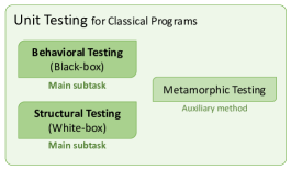
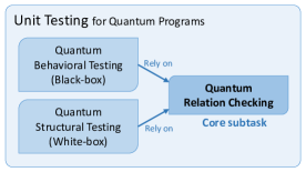
Figure 12. Unit testing in both classical and quantum programs comprises three subtasks and their interrelations.

6.4. Subtask A: Quantum Relation Checking

Given the challenges associated with generating and detecting quantum states, the indirect method of quantum relation checking plays a crucial role in testing quantum programs with multiple subroutines. As illustrated in Figure 12, the other two subtasks rely on this method. Quantum relations can be categorized into three types: (1) relations that pertain to statistical results; (2) relations that involve checking quantum states; and (3) relations that involve checking subroutines.

6.4.1. The relations about statistical results

One simple approach to testing quantum programs involves converting the target quantum states or programs into specific statistical results. The most commonly used statistical result is the probability distribution of the measurements. To illustrate, let us consider the output state $\left|+\right>=\frac{1}{\sqrt{2}}(\left|0\right>+\left|1\right>)$. By applying a measurement operation to this state, we can convert it into a Bernoulli distribution:

$$Pr[X=0]=\frac{1}{2}\hskip 11.38109ptPr[X=1]=\frac{1}{2}$$

We can repeat the execution of the target program many times, collect the measurement results, and then check whether the output results fit this distribution (i.e., the number of outputs ’0’s and ’1’s are nearly equal). Typically, the statistical results are obtained by repeatedly running the target programs, and existing statistical methods can then be used to analyze the results. For example, Huang and Martonosi (huang2019statistical, ) proposed statistical assertion methods for classical states, superposition states, and entanglements using hypothesis tests.

In addition to the probability distribution of measurements, parameter estimation is another commonly used technique for detecting quantum states. For instance, given two quantum states $\rho$ and $\sigma$ (which may be identical or different), the parameter $tr(\rho\sigma)$ can provide useful information. Several methods have been proposed for estimating $tr(\rho\sigma)$, such as the SWAP test (buhrman2001quantum, ; barenco1997stabilization, ) and Pauli measurements (cai2016optimal, ; gross2010quantum, ).

6.4.2. The relations about quantum states

The output states of quantum variables can be represented as state vectors or density matrices on paper. However, for quantum variables, there is a gap between the mathematical representation on paper and the testing process in quantum programs. Due to the challenges involved in generating and detecting quantum states (see Section 4.6), it is often necessary to convert the testing process into verifying specific relations about quantum states. The measurement probability distribution is one such relation that has already been discussed in the preceding section. In this section, we will discuss the relation between the quantum states themselves.

To illustrate this, let us consider the previous example of the output state $\left|+\right>=\frac{1}{\sqrt{2}}(\left|0\right>+\left|1\right>)$. As shown in Equation (7), it is noteworthy that applying the Hadamard gate to this state yields $\left|0\right>$:

(7) $$H\left|+\right>=\left|0\right>$$

Consequently, when measuring $\left|0\right>$, the outcome is always 0. Hence, if a measurement result of 1 occurs, it indicates that the output state is not $\left|+\right>$. This approach, known as deterministic-in-one-side judgment, avoids the need for repeated iterations too many times and enhances efficiency. The relation (7) serves as an effective means of verifying the output state $\left|+\right>$. In fact, several quantum runtime assertion methods (li2020projection, ; liu2020quantum, ; DBLP:conf/hpca/LiuZ21, ) are built upon this idea of deterministic-in-one-side relations. As this method involves transforming the target state into a simple classical state, such as $\left|0\right>$, it can also be called transform-based checking.

Generally, transform-based checking involves finding relations between the target quantum state and states that are easy to check. Here, we discuss the relations between pure states. Suppose that the expected output state is a pure state $\left|\psi_{eo}\right>$, which can be obtained by applying a simple unitary operation on an all-zero state, i.e., there exists a unitary operation $U_{eo}$ such that $\left|\psi_{eo}\right>=U_{eo}\left|0\ldots 0\right>$. If the practical output is $\left|\psi_{eo}\right>$, applying $U_{eo}^{-1}$ on it will result in an all-zero state; otherwise will not. The measurement result for the all-zero state is always 0, and the state will not be changed. From a testing perspective, $U_{eo}^{-1}$ is the inverse variant of $U_{eo}$ and can be easily implemented as long as $U_{eo}$ can be easily implemented. Compared to converting the output into a probability distribution, the most significant advantage of this method is that only one run is needed to obtain correct detection results with high probability. However, the disadvantage is that it is feasible only when a simple $U_{eo}$ of the expected state exists. If the implementation of $U_{eo}^{-1}$ is complex, this method may also be impractical. Example 6.3 provides a method to check the output of the QFT program under classical input states.

Example 6.0.

Output checking for the QFT program under the classical input states.

As shown in formula (3), the program specification of QFT (with BIBO endian mode) is as follows:

$$\begin{array}[]{c}\left|j_{1}\right>\rightarrow\frac{1}{\sqrt{2}}(\left|0\right>+e^{2\pi i0.j_{n}}\left|1\right>)\\ \cdots\\ \left|j_{n}\right>\rightarrow\frac{1}{\sqrt{2}}(\left|0\right>+e^{2\pi i0.j_{1}j_{2}\ldots j_{n}}\left|1\right>)\end{array}$$

Given classical state input $\left|j\right>=\left|j_{1}\right>\dots\left|j_{n}\right>$, the corresponding output state is the product state of $n$ single qubit states, each of which is represented in the form $\frac{1}{\sqrt{2}}(\left|0\right>+e^{i\theta_{j,k}}\left|1\right>)$, where $\theta_{j,k}=2\pi 0.j_{n-k+1}\ldots j_{n-1}j_{n}$ and can be generated by applying gate $U_{j,k}$ on $\left|0\right>$, where

(8) $$U_{j,k}=R_{1}(\theta_{j,k})H=\frac{1}{\sqrt{2}}\left[\begin{array}[]{cc}1&1\\ e^{i\theta_{j,k}}&-e^{i\theta_{j,k}}\end{array}\right]$$

To check the output, we use the transform-based method for applying $U_{j,k}^{-1}$ on the $k$-th qubit, and the overall operation is $U_{eo,j}^{-1}=U_{j,1}^{-1}\otimes\cdots\otimes U_{j,n}^{-1}$. If the output is correct, all qubits after applying $U_{j,k}^{-1}$ will become $\left|0\right>$, then the results of measured qubits will always be integer 0. Otherwise, non-zero results will be possible.

6.4.3. The relations about subroutines

Relations among subroutines are crucial in testing quantum programs, as they provide valuable insights into their correctness. When a target relation is satisfied, it indicates that the subroutines are likely correct. Conversely, if the relation is not satisfied, it indicates the presence of errors in at least one of the subroutines.

One commonly used relation is equivalence between two subroutines, which means that both subroutines produce the same output given the same input. Let us denote the two subroutines as $\texttt{P}_{1}$ and $\texttt{P}_{2}$, the equivalence relation can be expressed as $\texttt{P}_{1}=\texttt{P}_{2}$. A special case of equivalence is when a subroutine P is equal to an identity transform, denoted as $\texttt{P}=I$. In this case, the program specification for $I$ takes the following form:

(9) $$I:\left|x\right>\rightarrow\left|x\right>$$

Here, $I$ preserves the input state $\left|x\right>$ unchanged. Importantly, as we will discuss next, the notions of equivalence and identity serve as the foundation for many other useful relations in quantum program testing.

Quantum programs may consist of multiple subroutines, and in addition to the output states of these subroutines, there also exist relations among them that can be used for testing quantum programs. For example, consider the execution of several subroutines, denoted as $\texttt{P}_{1}$, $\texttt{P}_{2}$, …, $\texttt{P}_{n}$. We represent their sequential execution as the composed program $\texttt{P}_{n}\circ\dots\circ\texttt{P}_{2}\circ\texttt{P}_{1}$, where $\circ$ represents the sequential execution from right to left. It executes $\texttt{P}_{1}$ on input $x$ and produces output $o_{1}$, which becomes the input for $\texttt{P}_{2}$, and so on until the final output is produced by $\texttt{P}_{n}$.

A typical relation exists between an original subroutine and its variants. While some programming languages provide mechanisms for automatically generating and managing the three variants of an original program, these mechanisms may not always be available. Consequently, there are cases where it becomes necessary to manually implement these variants and test them. Fortunately, by leveraging the relation between the variants and the original subroutine, it is possible to avoid the need for redesigning test cases. This approach allows for a unified testing process that remains independent of the specific subroutine being tested. Suppose we have finished testing the original subroutine P, we denote inverse, controlled, power variants of P as InvP, CtrlP, and PowP, respectively.

For InvP, there is an obvious relation:

(10) $$\texttt{P}\circ\texttt{InvP}=I$$

where $I$ is the identity operation. Note that no matter what P is, the relation (10) is always held, so we obtain a unified test process for any InvP, that is, to execute the identity checking for the sequential execution of InvP and P.

The input of PowP contains two parts: the power $k$ (a classical integer) and target qubits qs. Given $k$, the effect on qs is equivalent to apply P (if $k>0$) or InvP (if $k<0$) for $|k|$ times. Also, the equivalence check can be converted into an identity check with the following identity relations:

(11) $$\begin{array}[]{cc}\texttt{InvP}^{k}\circ\texttt{PowP}(k)=I,&k>0\\ \texttt{P}^{|k|}\circ\texttt{PowP}(k)=I,&k<0\end{array}$$

Similarly, the input of CtrlP contains two parts: control qubits qctrl and target qubits qtar. If qctrl is in an all-one state $\left|1\ldots 1\right>$, then the effect on qtar is P. If qctrl is in a state which is orthogonal to $\left|1\ldots 1\right>$, then the effect is identity $I$. We can see that the testing of variants subroutines can be converted into the checking of identity and equivalence, which can be finished in unified processes.

In fact, equivalence checking and identity checking have classical counterparts, and classical equivalence is also a common relation among classical programs. However, we will discuss unitarity checking, which is quantum-specific and has no classical counterpart. Given a quantum subroutine P with IO type of transform. Unitarity checking is to check whether P represents a unitary transform. As we know, many typical quantum algorithms are unitary transforms, and measurement is the unique way to destroy the unitarity. Therefore, incorporating unitarity checking enables testers to identify unexpected measurement outcomes in the programs.

Unfortunately, to the best of our knowledge, no research has been conducted on the implementation of relation checking in testing tasks. This represents an open problem that deserves further research attention.

6.5. Subtask B: Quantum Structural Testing

As discussed in Sections 4.2.2 and 4.3.3, quantum programs may have specific structures that require careful checking to ensure correctness. In classical program testing, we commonly use branch coverage analysis to ensure the coverage of all possible control flow paths using selected input variables. However, in testing non-linear quantum programs, the execution path cannot be determined before running due to the uncertainty of quantum programs. Even the same input can lead to different execution paths in different running rounds, making it challenging to apply existing branch coverage methods for classical programs to quantum programs. In fact, the structure checking for general quantum programs is still an open problem, and further studies on control flows and branch coverage in quantum programs are essential to advance the field. In this paper, we focus on the overall testing process rather than specific testing techniques. Thus, we briefly discuss the structure checking for two typical quantum programs, the repeat-until-success (RUS, see Section 4.2.2) and the within-apply (WA, see Section 4.3.3), to provide insights into this crucial task.

To check the structure of a RUS program, the core step is to verify the loop’s termination condition. This condition is usually a predicate involving several classical variables, some of which may relate to the measurement results. Since we are only concerned with the program structure in this task, we can adopt a classical-quantum separation approach. Note that measurement is the only way for the quantum part to influence the classical part, and the condition relies only on the classical variables. Therefore, we can replace each measurement statement with a controllable classical parameter and remove all quantum parts to construct a testable substitute program that is purely classical and retains the structure of the original program. We can then perform the structure checking on this substitute program. An example of classical-quantum separation is shown in Example 6.4.

If the programming language supports WA syntax (such as Q#), the correctness of the WA structure is ensured by the language itself, and there is no need to check it separately. However, if the language does not support WA syntax, programmers need to implement three parts $U$, $V$, and $U^{-1}$, respectively. In this case, we need to ensure that the manual uncomputation is correct, i.e., $U^{-1}U=I$. This task can be transformed into an identity-checking problem.

Example 6.0.

The classical-quantum separation for Listing 2.

In Listing 2, we see a program with a RUS structure. The measurement statement is on Line 8, and m is the corresponding classical variable. Furthermore, m is also part of the termination condition (Line 9). To maintain classical-quantum separation, an additional parameter, set_inner_m, is introduced. We replace the measurement statement with this parameter and remove all quantum components to create the substitute. The code for the substitute is provided in Listing 7.

Listing 7: The classical substitute program of Listing 2.

⬇

1operation Random_0to2_Classical_Substitute(set_inner_m : Int) : Int {

2 //use qs = Qubit[2];

3 mutable m = 0;

4 repeat {

5 //Remove quantum parts

6 set m = set_inner_m; //Replace measurement statement with paremeter

7 } until (m < 3); //Success condition

8 //ResetAll(qs);

9 return m;

10}

6.6. Subtask C: Quantum Behavioral Testing

The task of program behavioral checking is to verify whether the behavior of the target program is consistent with its specification, which is typically achieved by running the target program with given inputs and observing whether the output matches the expected values. This subtask usually employs black-box testing, and appropriate inputs must be chosen. To accomplish this subtask, the IO mark of the target subroutine (see Section 4.4.1) must be obtained first, and its IO type (see Figure 8) will influence the design of the tests. Like testing classical programs, equivalence class partitioning and the combination of variables can be adopted to complete this subtask.

6.6.1. Equivalence Class Partition

Section 6.2.2 introduces two coarse-grained input partitioning principles, CSP and CSMP. However, for a specific target program, it is necessary to consider its logical meaning to construct a more effective partition. For instance, we can treat classical input states as classical integers and apply classical techniques like dividing by a boundary value to the partitioning process. Example 6.5 demonstrates an input partitioning and test case selection strategy for a phase-flip subroutine that, instead of simply partitioning the input space into classical and superposition states, we use the program specification to create a more elaborate partitioning scheme. The final equivalence classes are determined based on the program specification, and we also consider the detectability of the output as stated in (3) of Principle 1.

Example 6.0.

Input selection for the phase-flip subroutine.

Consider the conditional phase-flip subroutine PhaseFlip in the Grover Search program. It receives an input state qs = $\left|x\right>$ with $n$ qubits and outputs according to the value of $x$:

PhaseFlip : ($n$, qs) $\rightarrow$ (qs’)

(12) $$\texttt{PhaseFlip}:\left|x\right>\rightarrow\left\{\begin{array}[]{cc}-\left|x\right>&x>0\\ \left|x\right>&x=0\end{array}\right.$$

PhaseFlip keeps unchanged on all-zero input and flip phase on other classical state inputs. Note that the global phase cannot be distinguished by measurement, so classical state inputs will only get trivial results. To test whether it successfully flips the phase when $x=0$, we need to use the relative phase of the component in the superposition state. We choose input states in the form $\frac{1}{\sqrt{2}}(\left|x\right>+\left|y\right>)$, where $x$ and $y$ are chosen according to two branches in the formula (12). A feasible test strategy is to select the following four types of inputs:

• $\left|0\right>$;

• $\left|x_{1}\right>,x_{1}>0$;

• $\frac{1}{\sqrt{2}}(\left|0\right>+\left|x_{1}\right>),x_{1}>0$;

• $\frac{1}{\sqrt{2}}(\left|x_{1}\right>+\left|x_{2}\right>),x_{1},x_{2}>0,x_{1}\neq x_{2}$.

Types I and II are classical state inputs corresponding to the two branches of the formula (12); types III and IV are superposition state inputs, where type III is the superposition of the first branch and the second branch, and type IV is the superposition state of two states in the second branch. For input types, I, II, and IV, the difference between input and output should not be detected (same or at most global phase differences), and it ensures that the transformation is identical except for some global phases. The important case is input type III, in which the output state will be changed into $\frac{1}{\sqrt{2}}(-\left|0\right>+\left|x_{1}\right>)$. The difference between the output state and the input state can be detected.

6.6.2. Combination of Variables

Since many quantum programs have multiple input variables, it is also necessary to consider the combination of these variables during the testing process. Various combination coverage criteria between variables have been proposed for testing classical programs, such as All Combination Coverage (ACoC) (cohen1997aetg, ), Each Choice Coverage (ECC) (ammann1994using, ), Pair-wise Coverage (PWC) (burroughs1994improved, ), and Base Choice Coverage (BCC) (ammann1994using, ; cohen1994automatic, ). Obviously, these coverage criteria can be migrated into quantum program testing. Example 6.6 demonstrates how to combine classical and quantum input variables and select a feasible set of test inputs based on appropriate criteria. By applying these coverage criteria in the testing process, we can ensure that the combinations of input variables are thoroughly tested, improving the quality and reliability of the quantum program.

Example 6.0.

Equivalence class partitioning and combination for QFT program.

The IO mark of the QFT program is:

QFT : ($n$, qs) $\rightarrow$ (qs’)

As is shown in Listing 3, there are two loops in the QFT program, where the maximum index of the outer loop (line 21) is $n-2$, and the maximum index of the inner loop (line 23) is $n-1$. It is easy to see that 1 and 2 are two boundary values of $n$, so partition $n$ into three parts: $n=1$, $n=2$, and $n\geq 3$. We use the CSP criterion to partition qs into a classical state C and a superposition state S. To combine $n$ and qs, we use ACoC on these two parameters. Finally, there are six equivalence classes:

1. ($n=1$, C) 2. ($n=1$, S) 3. ($n=2$, C) 4. ($n=2$, S) 5. ($n\geq 3$, C) 6. ($n\geq 3$, S)

We select a concrete test input for each equivalence class. For the superposition state of qs, we use the STV criterion to select two-value-superposition states and use the SCAQ criterion to make the superposition cover all qubits. So we select complementary superposition states for S. A feasible set of tested input variables is:

• (1) $n=1$, $\mathrm{\mathbf{qs}}=\left|0\right>$

• (2) $n=1$, $\mathrm{\mathbf{qs}}=\frac{1}{\sqrt{2}}(\left|0\right>+i\left|1\right>)$

• (3) $n=2$, $\mathrm{\mathbf{qs}}=\left|01\right>$

• (4) $n=2$, $\mathrm{\mathbf{qs}}=\frac{1}{\sqrt{2}}(\left|00\right>+\left|11\right>)$

• (5) $n=7$, $\mathrm{\mathbf{qs}}=\left|1011001\right>$)

• (6) $n=6$, $\mathrm{\mathbf{qs}}=\frac{1}{\sqrt{2}}(\left|101101\right>+\left|010010\right>)$

6.7. Testing Cases and Execution

In classical testing, a test case is typically defined as a pair of inputs and expected outputs (ammann2016introduction, ), as shown in the following form:

Input: in_var_1, …, in_var_n

Expected output: out_var_1, …, out_var_m

Here, in_var_1, …, in_var_n are the given values assigned to all input variables, and out_var_1, …, out_var_m are the expected values for all output variables. However, in the case of quantum variables, simply specifying input and output values may not be sufficient. As discussed in Section 4.6, preparing or checking a quantum state described by a formula is not straightforward. Therefore, to ensure the effective testing of quantum programs, it is crucial to attach concrete methods for generating and checking target quantum states to the given quantum variables in the test cases. To this end, we propose the following principle:

Principle 4.

In each test case, attach the generation method for each quantum input state and the checking method for each quantum output state.

Following this principle ensures that the quantum variables in the test cases are executable, allowing for the evaluation of the correctness and accuracy of the quantum program under test.

In practice, the specific form of a test case for a quantum program may vary depending on the complexity and nature of the program. However, by adhering to the proposed principle, developers and testers can ensure that each test case is executable, allowing for effective testing and validation of the quantum programs. The generation method should specify the steps for preparing the input state, such as initializing qubits to a particular state or applying quantum gates to a set of qubits. The checking method should specify how to measure and verify the output state, such as performing quantum state tomography or measuring the expectation value of certain observables. Specifically, a test case for a quantum program has the following form:

Input:

cls_in_1, …, cls_in_$n_{ci}$,

[qs_in_1, GenProc_qs_in_1],

$\cdots$

[qs_in_$n_{qi}$, GenProc_qs_in_$n_{qi}$]

Expected Output:

cls_out_1, …, cls_out_$n_{co}$,

[qs_out_1, ChkProc_qs_out_1],

$\cdots$

[qs_out_$n_{qo}$, ChkProc_qs_out_$n_{qo}$]

Here, the values assigned to all input classical variables are denoted by cls_in_1, …, cls_in_$n_{ci}$, while the expected values for all output classical variables are denoted by cls_out_1, …, cls_out_$n_{co}$. For each quantum input item, such as [qs_in_1, GenProc_qs_in_1], it contains the input state qs_in_1 itself and the procedure GenProc_qs_in_1 indicating how to generate the target state. Similarly, for each quantum output item, ChkProc_qs_out_1 is the checking procedure for the target expected state qs_out_1.

The following Example 6.7 illustrates how to construct the set of test cases for the QFT program using the equivalence classes provided in Example 6.6.

Example 6.0.

Test cases for the QFT program.

At the end of Example 6.6, we give a feasible set of tested input variables. In the following, we describe how to expand this set to a set of executable test cases. Table 4 shows the input and the expected output pairs. We denote state $\left|\psi_{j}\right>$ as

(13) $$\left|\psi_{j}\right>=\frac{1}{\sqrt{2^{n_{j}}}}\sum_{k=0}^{2^{n_{j}}-1}e^{2\pi ijk/2^{n_{j}}}\left|k\right>$$

for any integer (binary string) $j$ with length $n_{j}$.

The checking for the output under the classical input has been discussed in Example 6.3. What remains is how to check the output with the state of the form $\frac{1}{\sqrt{2}}(\left|\psi_{a}\right>+\left|\psi_{b}\right>)$ (the last three items in Table 4), where $a$ and $b$ are two binary strings. There is no intuitive way to generate this state, but it has a useful property. For any $j$, suppose $U_{eo,j}\left|0\ldots 0\right>=\left|\psi_{j}\right>$. Then applying $U_{eo,a}^{-1}$ on the target state will get the following formula:

(14) $$U_{eo,a}^{-1}[\frac{1}{\sqrt{2}}(\left|\psi_{a}\right>+\left|\psi_{b}\right>)]=\frac{1}{\sqrt{2}}(\left|0\ldots 0\right>+U_{eo,a}^{-1}\left|\psi_{b}\right>)$$

where $\left|0\dots 0\right>\bot U_{eo,a}^{-1}\left|\psi_{b}\right>$ (since $\left|a\right>\bot\left|b\right>$ and unitary operations keep the orthogonality). Therefore, the probability of measuring this state to obtain an integer 0 is 1/2. This is similar to applying $U_{eo,b}^{-1}$. In order to check the output, we can repeat the following steps and count the number of results as 0 for the output.

• 1. Generate the input state $\frac{1}{\sqrt{2}}(\left|\psi_{a}\right>+\left|\psi_{b}\right>)$;

• 2. Run the target QFT program on the input state;

• 3. Apply $U_{eo,a}^{-1}$ or $U_{eo,b}^{-1}$;

• 4. Measure the output state.

If the number of results 0 occurs nearly half for both $U_{eo,a}^{-1}$ and $U_{eo,b}^{-1}$, we may be able to assume that the output state is as expected. In fact, due to the difficulty of checking a target output state, this is a compromise approach based on some properties of the target program, which we call the property-based testing method.

Table 4. A set of feasible test cases for the QFT program.

Equivalence Class	Input	Input Generation Procedure	Expected Output	Output Checking Procedure
($n=1$, C)	$\left|0\right>$	Algorithm 2	$\left|\psi_{0}\right>$1	See Example 6.3
($n=2$, C)	$\left|01\right>$		$\left|\psi_{01}\right>$
($n\geq 3$, C)	$\left|1011001\right>$		$\left|\psi_{1011001}\right>$
($n=1$, S)	$\frac{1}{\sqrt{2}}(\left|0\right>+i\left|1\right>)$	Apply $SH$ on $\left|0\right>$1	$\frac{1+i}{2}\left|0\right>+\frac{1-i}{2}\left|1\right>$	Apply $HS$ on output state1.
($n=2$, S)	$\frac{1}{\sqrt{2}}(\left|00\right>+\left|11\right>)$	Algorithm 3	$\frac{1}{\sqrt{2}}(\left|\psi_{00}\right>+\left|\psi_{11}\right>)$	See Example 6.7
($n\geq 3$, S)	$\frac{1}{\sqrt{2}}(\left|101101\right>+\left|010010\right>)$		$\frac{1}{\sqrt{2}}(\left|\psi_{101101}\right>+\left|\psi_{010010}\right>)$

• Note that the product of two gates in quantum computing is right-associative. $SH$ denotes applying the gate $H$ first, followed by the gate $S$, while $HS$ denotes applying the gate $S$ first, followed by the gate $H$.

In fact, checking the correctness of a quantum program solely based on output states under classical state input is not sufficient, but the behavior of the program with general input states can be complex and difficult to identify. Fortunately, if the target program is a unitary transform, its unitarity guarantees that the correctness of the classical state input implies the correctness of the general input. Therefore, a feasible approach to test a unitary program, denoted as P, is as follows:

• 1. Check the output states of P under classical input states;

• 2. Conduct additional unitarity checking for P.

By following these steps, the testing process incorporates the evaluation of superposition states within a unified unitarity checking framework, thereby reducing the burden on testers.

7. Integration Testing and Testing Practices

7.1. Integration Testing and Its Challenges

Just like classical programs, the correctness of individual subroutines in quantum programs does not necessarily guarantee the correctness of their composition. Bugs can occur in the interface between two subroutines, such as a mismatch in endian mode, as demonstrated in Example 7.1. Therefore, integration testing is also necessary for quantum programs.

Example 7.0.

A typical bug: the mismatch of the endian mode of two subroutines.

In classical computing, the endian mode is guaranteed by the computer architecture and is transparent to programmers. However, current quantum programming is still at the ”bit level” rather than the ”word level,” which means that we need to consider the operations on each qubit, and thus the endian mode (discussed in Section 4.4.3) must be guaranteed by programmers. The mismatch of the endian mode of two subroutines can lead to bugs. For instance, in Listing 4, the subroutine QFT in line 9 adopts the BIBO mode (Figure 9 (a)), and the corresponding index of qsclock in line 7 is ”n-i-1”. However, if the QFT subroutine in line 9 adopts the BILO mode (Figure 9 (b)), the correct index of qsclock in line 7 should be ”i.” This error is prone to occur, but challenging to reveal due to the limited support for endian mode in many quantum programming languages (as shown in Table 1), with even Q# currently providing only limited support.

Integration testing involves combining multiple subroutines within a quantum program. However, due to the constraints posed by the scale of executable quantum programs and the presence of noise, integration testing for quantum programs presents unique challenges compared to classical programs. The challenges in quantum integration testing can be categorized into two main aspects:

• Large Scale: Combined programs may be extensive, both in terms of the length of the execution series and the number of qubits required. Executing testing tasks on real hardware may be significantly impacted by decoherence and noise when dealing with long execution series. If we run these tasks on a simulator, using too many logic qubits may result in lengthy execution times.

• Non-Intuitive Partially Integrated Programs: Integration testing for quantum programs often involves testing partial or semi-finished programs. Describing these partially integrated stages for quantum programs may be challenging, making it difficult to design effective testing strategies.

7.2. Integration Order and the Usage of Test Doubles

In integration testing for quantum programs, determining the order of integration is the first step, which can be accomplished by applying strategies from classical integration testing, such as topological sorting. For instance, Example 7.2 demonstrates how to determine the integration order for QFT and QPE programs (as shown in Listings 3 and 4) based on their subroutine dependencies (as illustrated in Figure 14).

Example 7.0.

Determine the integration order of QFT and QPE programs.

Figure 14 illustrates the subroutine dependencies of the QFT and QPE programs, with direct callings represented by solid line arrows. Since Upower is an input parameter of QPE, it is not considered a direct calling, and we represent it as a dotted line arrow. Since there is no circular dependency and the subroutines are fixed except for Upower, we can employ topological sorting to determine feasible integration orders for the subroutines, excluding Upower. One example of a feasible integration order is

(1) CRk $\rightarrow$ (2) Reverse $\rightarrow$ (3) QFT $\rightarrow$ (4) QPE

The integration order in Example 7.2 is known as the bottom-up order. However, the Upower subroutine is abstract and unfinished in this code, and users need to replace it with a concrete subroutine. To do this, the test double technology used for testing classical programs (ammann2016introduction, ) can also be applied to quantum programs. A test double is a subroutine that replaces the original one while maintaining its essential properties for testing purposes but is easier to test. In fact, the substitute program created after classical-quantum separation, as discussed in Section 6.5, which retains the control flow structures but removes all quantum parts, is a typical example of a test double. Similarly, a quantum subroutine with an IO type of ”classical” can also be substituted by a pure-classical subroutine, as we will show in Section 9.2. The test double technique is also useful in the integration testing of quantum programs with oracles. Example 7.3 illustrates a strategy for testing a program that searches quantum memory using the Grover algorithm.

Example 7.0.

Testing a quantum program that searches quantum memory by the Grover algorithm.

This program has two subroutines: (1) general Grover search subroutine GS, accepting an oracle; (2) subroutine PO to implement the oracle of GS, which loads the quantum memory, compares the contents, and flips the phase of corresponding amplitudes. In the whole program, GS calls PO, as shown in Figure 14 (a).

We can adopt bottom-up order: test PO first and then combine it into GS. However, considering the effectiveness of locating bugs and the running cost (loading a quantum memory may be a costly operation), it is better to have individual testing for GS. In this case, the oracle PO is unfinished, and we should use test doubles to replace it. The test double can be implemented by some fixed unitary operations $U_{f}$:

$$U_{f}:\left|x\right>\rightarrow(-1)^{f(x)}\left|x\right>$$

where the indicator function $f$ is chosen and controlled by testers, as Figure 14(b). Compared with the original PO, $U_{f}$ avoids loading quantum memory. Using $U_{f}$, GS can be tested individually.

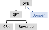
Figure 13. The subroutine dependencies of QFT and QPE programs in Listings 3 and 4.

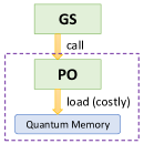
(a) Original Program

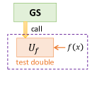
(b) Use test double $U_{f}$ to replace PO which loads quantum memory.

Figure 14. The usage of test doubles to reduce the cost of testing GS.

7.3. Testing Tools

In practice, testing quantum programs can be broken down into three steps: (1) writing testing scripts; (2) executing them on hardware or a simulator; and (3) analyzing the results. A testing script for a subroutine contains several testing cases, each of which involves generating input states and checking output states. Like testing classical programs, a well-designed testing tool can help test engineers complete testing tasks more efficiently. Based on the properties of quantum programs and the testing process mentioned above, we propose four basic functional requirements that a testing tool for multi-subroutine quantum programs should provide:

Principle 5.

The basic functional requirements of a testing tool for multi-subroutine quantum programs are as follows:

• 1. Repeated execution support for target programs;

• 2. Quantum information processing support;

• 3. Quantum subroutine composition support;

• 4. Results analysis support.

Let us discuss the necessity of these requirements. Requirement 1 is crucial because checking many quantum properties requires multiple copies of target states, which are the results of target programs. Therefore, the testing tool should provide a mechanism for running the target programs repeatedly. Requirement 2 is based on the discussion in Section 6.7, where we highlighted the importance of quantum information processing methods in generating test cases. Requirement 3 is essential for the integration testing of multi-subroutine quantum programs. Finally, requirement 4 is critical as a testing tool should not only output the experimental results but also provide necessary modules for result analysis. These four functions represent the minimum requirements for a testing tool, and a practical testing tool are allowed to provide additional features to meet specific needs.

7.4. Test-Driven Development: A Good Practice

Programming quantum systems can be challenging, and observing the values of quantum variables in real time can be difficult. To mitigate these challenges, it is helpful to detect bugs early in the development cycle, ideally during the development of each subroutine, rather than after the entire program is complete. In our research and development practice, we have found that a test-driven approach (beck2003test, ) facilitates early bug detection. This approach involves designing tests before development and then developing the subroutine to pass the tests. The method not only helps detect bugs early but also enhances the reliability of each subroutine, which increases developer confidence when working on large quantum programs with multiple subroutines.

Principle 6.

We encourage developers to embrace test-driven methods in the development of quantum programs. This approach involves designing tests before writing the actual code, and the primary objective of the development process is to ensure the successful passing of these tests.

8. Evaluation of Methods and Criteria for Unit Testing

We evaluate our testing framework in two steps. First, we evaluate our methods and criteria for unit testing using a set of benchmark subroutines in this section. Then we evaluate our complete testing process using three practical cases in the next section. For the evaluation of unit testing, we focus on the following research questions (RQs):

• RQ2: Are our unit testing design strategies effective for testing various quantum subroutines?

• RQ3: Is it necessary to cover both classical and superposition states as inputs to ensure adequate test coverage?

• RQ4: How effectively does the Superposition-Cover-All-Qubit (SCAQ) criterion reveal bugs in quantum programs?

8.1. RQ2: Case Studies for Designing Unit Testing

To address RQ2, we conducted case studies on various types of quantum subroutines.

8.1.1. Study cases

We have carefully selected a set of subroutines with relatively simple behavior, making them ideal candidates for unit testing. These subroutines cover all four input-output (IO) types and may have dependencies among each other. In the following, we provide a brief introduction to these 17 subroutines.

• IO type: classical

  • QRandom: Input an integer $n$, return a uniform random integer in $0,\dots,2^{n}-1$.

• IO type: generate-quantum

  • GenQInt: Input a binary string $x$ with length $n$. Generate $n$-qubit state $\left|x\right>$.

  • GenXPlusY: Input two binary strings $x$ and $y$ with length $n$. Generate $n$-qubit state $\frac{1}{\sqrt{2}}(\left|x\right>+\left|y\right>)$.

  • GenMaxSup: Generate $n$-qubit maximum superposition state.

  • GenMaxMix: Generate $n$-qubit maximum mixed state.

• IO type: detect-quantum

  • SwapTest: Input two subroutines which generate $n$-qubit states $\rho_{1}$ and $\rho_{2}$. Return their single-shot SWAP test result.

  • Purity: Input a subroutine that generates $n$-qubit state $\rho$ and the number of repeat $t$. Returns whether $\rho$ is a pure state. It uses SwapTest as its subroutine.

  • InnerProduct: Input two subroutines that generate $n$-qubit state $\rho_{1},\rho_{2}$ and the number of repeat $t$. Returns the estimation of $tr(\rho_{1}\rho_{2})$. It uses SwapTest as its subroutine.

• IO type: transform

  • Empty: A quantum circuit without any gate. It is equivalent to an identity transform.

  • Reverse: It reverse the order of input states. See lines $9\sim 16$ Listing 3.

  • MultiSWAP: It swaps quantum variables.

  • CRk: Subroutine of line $1\sim 7$ in Listing 3

  • PhaseFlip: See Example 6.5.

  • Grover: Given an oracle (implemented as an input subroutine), it performs the Grover Search algorithm. It contains PhaseFlip as its subroutine.

  • QFT: It performs the Quantum Fourier transform (see lines $18\sim 32$ in Listing 3).

  • QAdd: See formula (1).

  • Teleport: See Listing 1.

8.1.2. Design of testing plans

We conducted case studies by designing a unit testing plan for each subroutine. Our work results are summarized in Table 5, which involves analyzing the input-output (IO) mark and program specification of each subroutine and then designing the testing plan for each case based on the strategies outlined in Section 6. Regardless of the IO type, the IO mark can effectively represent the input and output variables of the target subroutine, allowing for clear differentiation between classical and quantum variables. In the testing design, we discuss equivalence class partitioning and provide corresponding test cases. Moreover, we include the generation methods for input quantum variables and the checking methods for output quantum variables. These case studies demonstrate the effectiveness of our unit testing design strategies for a variety of quantum subroutines.

Table 5. IO mark, program specification, and testing design for the benchmark subroutines.

Program	IO mark and Program Specification	Testing Design
QRandom	($n$) $\rightarrow$ (Int) return a uniform random integer in $[0,2^{n}-1]$	Equivalence classes: $n=0$, $n>0$ Test cases: [input: $n$ = 0; output: 0$\sim$1] [input: $n$ = 5; output: 0$\sim$31] Check outputs: Property-based checking for the output range.
GenQInt	($n$, $x$) $\rightarrow$ (qs’) return $\left|x\right>$ ($n$ qubits)	Test cases: [input: $n=5,x=0$; output: $\left|00000\right>$] [input: $n=6,x=23$; output: $\left|010111\right>$] Check output: Measure qs’ and compare the result with input $x$.
GenXPlusY	($n$, $x$, $y$) $\rightarrow$ (qs’) return $\frac{1}{\sqrt{2}}(\left|x\right>+\left|y\right>$)	Equivalence class: $x=y$, $x\neq y$. Test cases: [input: $n=5$, $x=y=20$; output: $\left|10100\right>$] [input: $n=4$, $x=5$, $y=12$; output: $\frac{1}{\sqrt{2}}(\left|0101\right>+\left|1100\right>)$] Check output: Measure qs’ and compare the result with $x$ and $y$.
GenMaxSup	($n$) $\rightarrow$ (qs’) return $\frac{1}{\sqrt{2^{n}}}\sum_{x\in\{0,1\}^{n}}\left|x\right>$	Test cases: [input: $n=1$; output: $\left|+\right>$] [input: $n=5$; output: $\left|+++++\right>$] Check output: Apply $H^{\otimes n}$ on the output qs’ and measurement.
GenMaxMix	($n$) $\rightarrow$ (qs’) return $\frac{1}{2^{n}}\sum_{x\in\{0,1\}^{n}}\left|x\right>\left<x\right|$	Test cases: [input: $n=1$; output: $\frac{1}{2}\left|0\right>\left<0\right|+\frac{1}{2}\left|1\right>\left<1\right|$] [input: $n=32$; output: $\rho_{out}=\frac{1}{2^{5}}I_{32}$] Check output: Measure qs’ and check whether the output range is $0\sim 2^{n}-1$.
SwapTest	($n$, GenRho1, GenRho2) $\rightarrow$ (Result) return once SWAP test result	Equivalence classes: CSMP for $\rho_{1}$ and $\rho_{2}$; $\rho_{1}=\rho_{2}$ or $\rho_{1}\neq\rho_{2}$. Test cases: [input: $\rho_{1}=\left|011\right>\left<011\right|$, $\rho_{2}=\left|110\right>\left<110\right|$; return 0 with $p_{0}=0.5$] [input: $\rho_{1}=\rho_{2}=\left|1001\right>\left<1001\right|$; return 0 with $p_{0}=1$] [input: $\rho_{1}=\left|0\right>\left<0\right|$, $\rho_{2}=\left|+\right>\left<+\right|$; return 0 with $p_{0}=0.75$] [input: $\rho_{1}=\rho_{2}=\frac{1}{2}\left|0\right>\left<0\right|+\frac{1}{2}\left|1\right>\left<1\right|$; return 0 with $p_{0}=0.75$] [input: $\rho_{1}=\left|+\right>\left<+\right|$, $\rho_{2}=\frac{1}{2}\left|0\right>\left<0\right|+\frac{1}{2}\left|1\right>\left<1\right|$; $p_{0}=0.75$] Generate input: Use Algorithms 2, 4, and 7. Check output: Repeat several times and count the proportion of result 1.
textttPurity	($n$, $t$, GenRho) $\rightarrow$ (isPure) return TRUE if $\rho$ is pure state.	Equivalence classes: $\rho$ is classical, superposition and mixed. Test cases: [input: $\rho:\left|0101\right>$, $t=100$; output: True] [input: $\rho:\frac{1}{\sqrt{2}}(\left|00\right>+\left|11\right>)$, $t=100$; output: True] [input: $\rho=\frac{1}{2}\left|0\right>\left<0\right>+\frac{1}{2}\left|1\right>\left<1\right>$, $t=100$; output: False] Generate input: Use Algorithms 2 and 4. Check output: The expected output is returned with high probability.
InnerProduct	($n$, $t$, GenRho1, GenRho2) $\rightarrow$ (Float) return estimation of $tr(\rho_{1}\rho_{2})$	Equivalence classes: CSMP for $\rho_{1}$ and $\rho_{2}$; $\rho_{1}=\rho_{2}$ or $\rho_{1}\neq\rho_{2}$. Test cases: [input: $\rho_{1}=\left|0011\right>\left<0011\right|$, $\rho_{2}=\left|1010\right>\left<1010\right|$; output: $\sim 0$] [input: $\rho_{1}=\rho_{2}=\left|1001\right>\left<1001\right|$; output: $\sim 1$] [input: $\rho_{1}=\left|0\right>\left<0\right|$, $\rho_{2}=\left|+\right>\left<+\right|$; output: $\sim 0.5$] [input: $\rho_{1}=\rho_{2}=\frac{1}{2}\left|0\right>\left<0\right|+\frac{1}{2}\left|1\right>\left<1\right|$; output: $\sim 0.5$] [input: $\rho_{1}=\left|+\right>\left<+\right|$, $\rho_{2}=\frac{1}{2}\left|0\right>\left<0\right|+\frac{1}{2}\left|1\right>\left<1\right|$; output: $\sim 0.5$] Generate input: Use Algorithms 2, 4, and 7.

Continued from Table 5

Program	IO mark and Program Specification	Testing Design
Empty	($n$, qs) $\rightarrow$ (qs’) $\left|\psi\right>$ $\rightarrow$ $\left|\psi\right>$	Use identity checking.
Reverse	($n$, qs) $\rightarrow$ (qs’) $\left|j_{1}\right>\dots\left|j_{n}\right>\rightarrow\left|j_{n}\right>\dots\left|j_{1}\right>$	Equivalence classes: $n=1$; $n>1$ is odd; $n$ is even. Test cases: [input: $\left|1\right>$, output: $\left|1\right>$] [input: $\left|11001\right>$, output: $\left|10011\right>$] [input: $\left|010011\right>$, output: $\left|110010\right>$] Generate input: Use Algorithm 2. Check output: Use the inverse of Algorithm 2. Additional unitarity checking.
MultiSWAP	($n$, qs1, qs2) $\rightarrow$ (qs1’, qs2’) $\left|\phi\right>\left|\psi\right>\rightarrow\left|\psi\right>\left|\phi\right>$	Take random testing. Generate input: $(U_{\phi}\otimes U_{\psi})\left|0\right>\otimes\left|0\right>$, with randomly chosen $U_{\phi}$ and $U_{\psi}$. Check output: Apply $U_{\psi}\otimes U_{\phi}$ on the output state and measurement. Compare the measurement result with 0.
CRk	($k$, qctrl, qtar) $\rightarrow$ (qctrl’, qtar’) $\left|c\right>\left|\psi\right>\rightarrow\left|c\right>\left[\begin{array}[]{cc}1&0\\ 0&\exp\left(\frac{i\pi c}{2^{k}}\right)\\ \end{array}\right]\left|\psi\right>$	Equivalence classes: $c=0$; $c=1$. Test cases: [input: $k=2$, $\left|0\right>\left|+\right>$; output: $\left|0\right>\left|+\right>$] [input: $k=1$, $\left|1\right>\left|+\right>$; output: $\frac{1}{\sqrt{2}}\left|1\right>(\left|0\right>+i\left|1\right>)$] Generate input and check output: See Example 6.3.
PhaseFlip	($n$, qs) $\rightarrow$ (qs’) $\left|x\right>\rightarrow\left\{\begin{array}[]{cc}-\left|x\right>&x>0\\ \left|x\right>&x=0\end{array}\right.$	Equivalence classes: $n$: ’$=1$’ , ’$>1$’; qs: see Example 6.5. Test cases: [input: qs=$\left|0\right>$; output: $\sim$input] [input: qs=$\left|1\right>$; output: $\sim$input] [input: qs=$\left|+\right>$; output: $\neq$input] [input: qs=$\left|00000\right>$; output: $\sim$input] [input: qs=$\left|01101\right>$; output: $\sim$input] [input: qs=$\frac{1}{\sqrt{2}}(\left|00000\right>+\left|11001\right>)$; output: $\neq$input] [input: qs=$\frac{1}{\sqrt{2}}(\left|0110\right>+\left|1001\right>$); output: $\sim$input] Generate input: Use Algorithms 2 and 4. Check output: Equivalence checking for input and ouput of qs.
Grover	($n$, OracleK) $\rightarrow$ (qs’) return $\approx\left|K\right>$	Take random testing. Generate input: Randomly choose integer $K$ and construct OracleK. Check output: Measure qs’ and the result should be $K$ with high probability.
QFT	($n$, qs) $\rightarrow$ (qs’) $\left|j\right>\rightarrow\frac{1}{\sqrt{2^{n}}}\sum_{k=0}^{2^{n}-1}e^{2\pi ijk/2^{n}}\left|k\right>$	Equivalence classes: see Example 6.6. Test cases: see Example 6.7. Generate input and checking output: See Example 6.3 and Example 6.7.
QAdd	($n$, qs1, qs2) $\rightarrow$ (qs1’, qs2’) $\left|x\right>\left|y\right>\rightarrow\left|x\right>\left|x+y\right>$	Equivalence classes: Result overflow / not overflow. Test cases: [input: $\left|0011\right>\left|0110\right>$, output: $\left|0011\right>\left|1001\right>$] [input: $\left|1100\right>\left|1001\right>$, output: $\left|1100\right>\left|0111\right>$] Generate input: Use Algorithm 2. Check output: Use the inverse of Algorithm 2; Additional unitarity checking.
Teleport	(qsrc) $\rightarrow$ (qdest’) $\left|q\right>\rightarrow\left|q\right>$	Use identity checking

8.2. Mutation Programs

RQ3 and RQ4 focus on evaluating the effectiveness of testing principles or criteria for identifying erroneous programs. One common approach to simulate bugs in practical programs is through mutation. For multi-subroutine quantum programs, it is valuable to consider four types of mutations:

• Gate Mutation (GM): This involves adding, removing, or modifying a basic quantum gate.

• Subroutine Mutation (SM): This type of mutation involves adding, removing, or modifying a calling statement. In the case of modification, it refers to making the calling statement invoke an erroneous version of the original subroutine.

• Classical Mutation (CM): It focuses on modifying control-flow statements, classical expressions, or assignments of classical variables.

• Measurement Mutation (MM): This mutation type involves adding or removing measurement statements.

Figure 15 provides specific examples of these four types of mutations applied to an original subroutine. Previous research on testing quantum programs (ali2021assessing, ; wang2021generating, ; wang2021application, ; fortunato2022qmutpy, ; fortunato2022mutation, ) and quantum platforms (wang2021qdiff, ) has mainly considered gate mutation (GM) and measurement mutation (MM). This paper introduces two new mutation types - subroutine mutation (SM) and classical mutation (CM), which are essential for evaluating multi-subroutine and quantum-classical mixed programs.

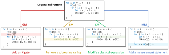
Figure 15. Examples about gate mutation (GM), subroutine mutation (SM), classical mutation (CM), and measurement mutation (MM).

8.3. RQ3 and RQ4: Experimental Design

To address RQ3 and RQ4, we have selected six subroutines from Section 8.1 with an IO type of ”transform.” As shown in Table 6, for Reverse, MultiSWAP, and QFT, we consider different scales $n$. Our objective is to evaluate the necessity of covering both classical and superposition states and the effectiveness of the SCAQ criteria using mutation testing techniques.

In the row labeled ”#mutations,” we have constructed several mutations for each original correct subroutine, including Gate Mutation (GM), Subroutine Mutation (SM), Classical Mutation (CM), and Measurement Mutation (MM), as discussed in Section 8.2. Each mutation subroutine used in the evaluation consists of only one mutation, affecting one line of code, and can be successfully compiled. We have ensured that the mutations cover all parts of the original subroutine uniformly, with each type of mutation including adding, deleting, and replacing operations.

For the evaluation, we have employed random testing, where we randomly generate input cases of specific types for each mutation and check whether the case can trigger errors in the mutation. We consider three types of input states: classical input (CI), represented as $\left|x\right>$ with a random integer $x$; random two-value superposition input (RTI), represented as $\frac{1}{\sqrt{2}}(\left|x\right>+\left|y\right>)$ with two random integers $x$ and $y$; and complementary superposition input (CSI), represented as $\frac{1}{\sqrt{2}}(\left|x\right>+\left|\bar{x}\right>)$ with a random integer $x$ and its bitwise negation $\bar{x}$. To check the output, we use transform-based checking for RTI and CSI of QFT, and the method described in Section 6.4.2 for CI of QFT and other subroutines. For a fair comparison, we perform each transform-based checking only once and record the trigger result directly. It is important to note that the trigger rate observed in this evaluation may not reflect the rates encountered in practical testing tasks. In practical scenarios, multiple repetitions are often performed to enhance the accuracy of the judgment. Additionally, due to the larger input space with increasing scale $n$, we have selected the number of cases for each mutation to be $100n$ to cover a broader range of scenarios adequately. This selection is based on empirical grounds.

We have used the Q# language and its simulator for our experiments, as (1) our methods and benchmark programs involve variable-scale and classical-quantum-mixed scenarios, and (2) Q# is a high-level quantum programming language that supports such program patterns. The experiments were conducted on a personal computer equipped with an Intel Core i7-1280P CPU and 16 GB RAM.

The results of the experiments are presented in Table 6, which consists of five subtables. Subtable (a) provides the parameters of the tested subroutines, mutations, and test cases. Subtables (b), (c), and (d) display the trigger numbers and trigger rates of each mutation under CI, RTI, and CSI, respectively. Subtable (e) presents the overall trigger rates for each subroutine.

8.4. RQ3: The Necessity of Covering Both Classical and Superposition States

According to the subtables (b), (c), and (e) in Table 6, we observe that for most mutations, the trigger rate is higher for RTI compared to CI. Interestingly, the trigger rate of MMs using classical input states is significantly lower than that of MMs using superposition input states. Particularly for CRk, Empty, Reverse, and MultiSWAP, classical input states fail to trigger any MMs. Further investigation reveals the following findings: (1) If the program consists of ”essentially classical” gates (such as X, CNOT, and SWAP), classical input states cannot trigger any MMs. This is because, under classical input states, the computation process remains essentially classical, and measurements do not alter the variable contents. (2) If the MM occurs at the beginning of a program, classical input states are unable to trigger it since measurements do not modify the given input. (3) Certain ”phase-only” mutations (such as adding an S or Z gate) cannot be triggered by classical input states.

Another intriguing observation relates to the trigger rate with scale $n$. For cases where $n=1$, the trigger rate for each program is consistently low. This can be attributed to the absence of loop executions at $n=1$, resulting in mutations inside loops not being triggered. By examining the results of the $n=1$ test cases, we can determine whether bugs are located inside or outside the loops.

During the execution of the experiments, it is worth noting that some mutations fail due to exceptions rather than output checking, with most of these cases involving CMs. In practice, mutations in classical parameters, such as array indices, can be triggered by exceptions through the exception-handling mechanisms present in programming languages.

While superposition input states demonstrate higher trigger rates compared to classical input states, this does not imply that we should solely focus on testing superposition inputs. In fact, checking output under superposition input states usually relies on checking output under classical input states (as demonstrated in Example 6.7). Additionally, we also observed that certain mutations triggered by classical input states fail to be triggered by superposition input states. This highlights the crucial role of superposition as a differentiating factor between classical and quantum computing. Therefore, it is necessary to cover both classical and superposition inputs when testing quantum programs.

Table 6. The evaluation results of RQ3 and RQ4

(a) Experiments configurations
		CRk	Teleport	Empty	Reverse			MultiSWAP		QFT
#mutations	GM	6	13	9	16			13		20
	SM	0	0	0	0			0		16
	CM	4	12	0	12			8		18
	MM	4	7	2	10			10		12
parameter $n$		-	-	10	1	8	9	1	6	1	2	6
#total qubits		2	3	10	1	8	9	1	12	1	2	6
#cases for each mutation		200	100	1000	100	800	900	100	600	100	200	600
#cases	GM	1200	1300	9000	1600	12800	14400	1300	7800	2000	4000	12000
	SM	-	-	-	-	-	-	-	-	1600	3200	9600
	CM	800	1200	-	1200	9600	10800	800	4800	1800	3600	10800
	MM	800	700	2000	1000	8000	9000	1000	6000	1200	2400	7200
#total cases		1400	3200	11000	3800	30400	34200	3100	18600	6600	13200	39600
(b) The number of mutations triggered by classical input (CI)
#trigger by CI	GM	224	436	4999	348	9262	10473	868	6860	300	2068	9900
	SM	-	-	-	-	-	-	-	-	52	1530	7771
	CM	248	461	-	300	8094	9598	353	4442	154	1781	9545
	MM	0	56	0	0	0	0	0	0	240	1087	4725
Trigger rate by CI (%)	GM	18.7	33.5	55.6	21.8	72.4	72.7	66.8	87.9	15.0	51.7	82.5
	SM	-	-	-	-	-	-	-	-	3.3	47.8	80.9
	CM	31.0	38.4	-	25.0	84.3	88.9	44.1	92.5	8.6	49.5	88.4
	MM	0.0	8.0	0.0	0.0	0.0	0.0	0.0	0.0	20.0	45.3	65.6
(c) The number of mutations triggered by random two-value superposition input (RTI)
#trigger by RTI	GM	241	569	6220	442	10912	12353	338	7202	615	2898	11625
	SM	-	-	-	-	-	-	-	-	19	2599	8954
	CM	260	453	-	300	8515	9995	300	4576	219	2183	10762
	MM	201	208	788	200	3287	3766	524	2848	12	1540	5424
Trigger rate by RTI (%)	GM	20.1	43.8	69.1	27.6	85.3	85.8	26.0	92.3	30.8	72.5	96.9
	SM	-	-	-	-	-	-	-	-	1.2	81.2	93.3
	CM	32.5	37.8	-	25.0	88.7	92.5	37.5	95.3	12.2	60.6	99.6
	MM	25.1	29.7	39.4	20.0	41.1	41.8	52.4	47.5	1.0	64.2	75.3
(d) The number of mutations triggered by complementary superposition input (CSI)
#trigger by CSI	GM	610	603	7414	452	12249	13901	938	7775	615	3294	11611
	SM	-	-	-	-	-	-	-	-	13	2804	8865
	CM	358	441	-	300	8071	9628	683	4781	215	2310	10799
	MM	387	212	1014	211	4035	4487	748	5963	19	1786	5417
Trigger rate by CSI (%)	GM	50.8	46.4	82.4	28.3	95.7	96.5	72.2	99.7	30.1	82.4	96.8
	SM	-	-	-	-	-	-	-	-	0.8	87.6	92.3
	CM	44.8	36.8	-	25.0	84.1	89.1	85.4	99.6	11.9	64.2	99.99
	MM	48.4	30.3	50.7	21.1	50.4	49.9	74.8	99.4	1.6	74.4	75.2

(e) The overall trigger rates of six subroutines with three types of input: CI, RTI, and CSI

8.5. RQ4: The Effectiveness of Superposition Covering All Qubits

According to the subtables (c), (d), and (e) in Table 6, it can be observed that CSI has a higher trigger rate than RTI, even though both are superposition input states. This indicates that superposition with a larger extent has a greater ability to reveal bugs compared to superposition with a lower extent. Actually, this result can be attributed to the occurrence possibility of mutations on every qubit, coupled with the comprehensive coverage of the input superposition facilitated by the SCAQ criterion. Furthermore, we have noticed that different subroutines exhibit varying degrees of sensitivity to trigger rates with RTI and CSI. Specifically, CRk and MultiSWAP demonstrate sensitivity, while Teleport and QFT do not exhibit the same level of sensitivity. Nevertheless, in general, test cases that satisfy the SCAQ criterion prove to be more effective in uncovering bugs.

9. Case Studies for Complete Testing Process

In this section, we evaluate the effectiveness of our overall testing process by conducting case studies on three representative multi-subroutine quantum programs. Our objective is to answer the following research question:

• RQ5: Are our testing design strategies effective for testing multi-subroutine quantum programs?

For each case study, we will present an overview of the program’s design along with its corresponding Q-UML diagram. Subsequently, we will delve into the testing design, with a particular emphasis on integration testing. This analysis will allow us to assess the efficacy of our testing approach in the context of multi-subroutine quantum programs.

9.1. Case 1: Quantum Phase Estimation (QPE)

The program structure and subroutine dependency of QPE were discussed in Example 7.2. It is based on QFT and requires an input target subroutine called Upower. According to its IO mark (see Example 6.1), it has four input variables: Nclock, Ntarget, Upower, and target. We follow a bottom-up order, first testing the subroutine QFT, then proceeding to test QPE itself. The steps involved are as follows:

• Unit test for QFT.

• Equivalence class partition for each input variable:

  • Partition: Nclock[ins, suf]; Ntarget[=1, $\geq$2]; Upower[fev, ifev]; target[es, nes].

• Combination for input variables:

  • Combination criterion: ECC.

  • A set of feasible equivalence classes:

    • (Nclock is suf, Ntarget = 1, Upower is fev, target is es)

    • (Nclock is suf, Ntarget = 1, Upower is fev, target is nes)

    • (Nclock is suf, Ntarget $\geq$ 2, Upower is fev, target is es)

    • (Nclock is suf, Ntarget $\geq$ 2, Upower is fev, target is nes)

    • (Nclock is ins, Ntarget $\geq$ 2, Upower is ifev, target is es)

• Construct a set of feasible test cases:

  • [input: Ntarget=1, Nclock = 3, Upower$=X$, target$=\left|-\right>$;

    output: target’$=\left|100\right>$ ]

  • [input: Ntarget=1, Nclock = 3, Upower$=H$, target$=\left|0\right>$;

    output: target’: $\left|000\right>$ with prob $\sim 0.8536$, $\left|111\right>$ with prob $\sim 0.1464$ ]

  • [input: Ntarget=3, Nclock = 3, Upower$=Controlled(S\otimes S^{\dagger})$, target$=\left|101\right>$;

    output: target’$=\left|110\right>$ ]

  • [input: Ntarget=3, Nclock = 3, Upower$=Controlled(S\otimes S^{\dagger})$, target$=\frac{1}{\sqrt{2}}(\left|101\right>+\left|110\right>)$;

    output: target’: $\left|110\right>$ with prob $\sim 0.5$, $\left|010\right>$ with prob $\sim 0.5$ ]

  • [input: Ntarget=2, Nclock = 7, Upower$=ControlledR_{z}(\frac{2}{3}\pi)$, target$=\left|10\right>$;

    output: target’$=\left|x\right>$, $x\approx\frac{5}{6}$ ]

• Owing that Upower is an input subroutine, we need to implement each Upower in the test cases.

• Run test cases given in step (4).

9.2. Case 2: Shor’s Factoring Program (Shor)

9.2.1. Program Structure

The Shor program is designed to factorize a positive integer $N$ and produce the factorization series of $N$. The program’s structure is represented by the Q-UML diagram shown in Figure 17. We have modeled the program using several Q-UML classes. The core module is the order-finding class QOrderFinding. This class takes a positive integer $x$ as input and determines its order $r$, the minimum value of $r$ satisfying the equation $x^{r}\equiv 1(\mathrm{mod}\hskip 2.84526ptN)$. The QOrderFinding class consists of three subroutines: QPhaseEstimation, which performs quantum phase estimation, QModularMultiply, which implements the transform $\left|y\right>\rightarrow\left|xy(\mathrm{mod}\hskip 2.84526ptN)\right>$, and a classical subroutine for continued fraction calculations. As discussed in Section 3.2, the Shor program incorporates order finding and other number theory subroutines such as greatest common factors (GCD) and a check for whether $N$ is in the form of $a^{b}$. These subroutines are encapsulated within the FactorTest class. At the top level, the Application class provides the user interface for the program.

9.2.2. Testing Design

It is important to note that the subroutines upper than QOrderFinding are classical in nature and can also be implemented as a classical version called COrderFinding. By replacing QOrderFinding with COrderFinding, the program Shor transforms into a classical factoring program named CShor that relies on classical order finding. Therefore, test double technology is suitable for the subroutines above the order-finding process. In practice, the following steps can be followed to complete the testing task:

• Perform unit tests for classes QModularMultiply, QPhaseEstimation, ContinuedFraction, and
  FactorTest.

• Test QOrderFinding using a bottom-up integration order.

• Utilize test double technology by replacing the invocation of QOrderFinding in the Shor class with COrderFinding. The modified class, denoted as CShor, exhibits the same external behavior as Shor, which can be ensured through classical equivalence checking.

• CShor represents a classical factoring program based on classical order finding. Employ classical methods to test its correctness. This step ensures the correctness of Shor except for the QOrderFinding subroutine.

• Conduct testing on Shor and the entire Application program.

In this testing plan, COrderFinding serves as a test double, allowing the testing of upper-level classes to be performed without requiring quantum resources.

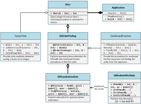
Figure 16. The Q-UML diagram illustrating the structure of the demo program for Shor’s algorithm.

Figure 17. The Q-UML diagram illustrating the structure of the demo program for solving a linear system.

9.3. Case 3: Linear System Solver

9.3.1. Program Structure

Consider a quantum linear system solver program for $Ax=b$. It allows users to provide the matrix $A$ using a sparse representation (as the sum of several Pauli operators) and $b$ through a state-generation operation. The program utilizes the HHL algorithm to solve the system and performs measurements on the output state a given number of times. The resulting distribution of each measurement outcome is then presented. Figure 17 illustrates the Q-UML diagram of the program. To represent the matrix $A$, a data-structural class called PauliSum is employed to pass parameters from the LinearSystemSolver class to the HamiltonianSimulation class. In this application, phase estimation is utilized for the Hamiltonian simulation, and the core module of the HHL algorithm is implemented in the ControlledRotation class. The HHLCore class implements the HHL circuit depicted in Figure 4, while the LinearSystemSolver class encompasses the program’s running parameters and calls the HHLCore class.

9.3.2. Testing Design

Note that the topmost class, Application, includes a display function. This display function can be reconstructed to a function for checking the results, which can serve as a testing fixture for lower-level classes. Therefore, we adopt a combination of bottom-up and top-down integration strategies, following the steps outlined below:

• Perform unit testing for the lower-level classes, such as ControlledRotation, QPhaseEstimation, and HamiltonianSimulation.

• Test the topmost class Application, and subsequently reconstruct the display function to a dedicated function for checking the results.

• Integrate the HHLCore and LinearSystemSolver classes into Application. Throughout the integration process, the testing results can be examined using the result-checking function developed in step (2).

By combining bottom-up and top-down approaches and leveraging the result-checking function, we ensure comprehensive testing coverage for the entire program.

9.4. Insights Learned from the Case Studies

Towards the conclusion of this section, we share valuable insights gained from the case studies.

$\bullet$ Insight 1: In the top-down integration, quantum subroutines with an IO type of ”classical” can be substituted with equivalent classical subroutines.

Many quantum algorithms are designed to tackle traditional problems, such as factoring, through algorithms like Shor’s algorithm. These algorithms typically involve a combination of quantum subroutines at the lower level and classical subroutines at the top level. The connection between the two is established through a quantum subroutine with an IO type of ”classical”, which bridges the quantum and classical components. In this scenario, it is possible to replace the quantum subroutines with equivalent classical subroutines, transforming the entire target program into an equivalent classical program. This approach allows for utilizing existing classical testing technologies in the top-down integration process. For instance, as demonstrated in Section 9.2, the quantum subroutine QOrderFinding can be substituted with a classical equivalent subroutine COrderFinding, enabling the implementation of top-down integration.

$\bullet$ Insight 2: If feasible, it is recommended to prioritize the adoption of transform-based methods for checking the running output.

As discussed in the previous section, there are two main methods for checking the output: (a) the statistic-based method, which involves running the target programs multiple times and collecting statistical results; and (b) the transform-based method, which applies additional unitary and measurement operations to the output to check for unexpected results. Method (a) requires a large number of repetitions to achieve high accuracy, resulting in decreased efficiency. On the other hand, method (b) allows us to identify errors when unexpected results occur, but its implementation can be challenging in certain cases due to the complexity of the required transform. Our case studies also demonstrate that method (b) is more efficient than method (a) whenever it can be successfully implemented. Therefore, we recommend prioritizing the use of transform-based methods to check the running output whenever feasible.

$\bullet$ Insight 3: A recommended testing approach is systematically increasing the testing scale, starting from small-scale scenarios and gradually progressing to larger ones.

Many quantum programs, including those with variable scales such as QFT (Quantum Fourier Transform), rely on a parameter $n$ representing the number of qubits involved. In order to ensure efficient testing, we recommend a step-by-step approach, starting from small-scale scenarios and gradually progressing to larger scales. For instance, referring to the Table 4 provided, testing QFT would involve examining three cases of $n$: $n=1$, $n=2$, and $n\geq 3$. An effective strategy is, to begin with the smallest scale, testing the $n=1$ case and promptly reporting any discovered bugs to the developers. Once the identified errors have been rectified (i.e., the $n=1$ case passes), the testing can then proceed to the $n=2$ case. Finally, the $n\geq 3$ case can be tested. This sequential order is recommended as smaller-scale programs typically execute more quickly, enabling the timely detection and resolution of errors.

10. Conclusion And Future Work

This paper has presented a systematic and comprehensive approach to testing multi-subroutine quantum programs. By investigating the key properties of quantum programs and considering their unique characteristics, we have developed a testing process that encompasses unit testing and integration testing. The proposed testing principles and criteria provide guidance for designing effective test cases and ensuring the reliability of quantum programs. Through extensive evaluation and case studies on typical quantum subroutines, we have demonstrated the effectiveness of our testing processes, principles, and criteria in detecting bugs and ensuring the correctness of multi-subroutine quantum programs.

However, there are several open problems that require further research:

• Concrete checking algorithms for important quantum relations: Developing specific algorithms to verify essential quantum relations, such as identity, equivalence, and unitarity, which are highlighted in Section 6.4.3, is crucial for facilitating the testing of quantum programs.

• Structural testing for general quantum programs: Quantum programs pose challenges for structural testing due to uncertain execution paths. New methods are needed to accurately describe these paths and measure the coverage rates of quantum programs.

• Testing research on practical quantum software systems: As practical quantum software systems emerge, it is important to evaluate the effectiveness of existing testing methods and explore the development of new methods tailored to the unique challenges of quantum programming.

• Testing processes at higher levels: While this paper focuses on unit testing and integration testing, testing at higher levels, such as system testing, is crucial for ensuring the overall correctness and reliability of quantum software systems. Future research should explore testing processes at these higher levels.

Addressing these open problems will contribute to the advancement of testing techniques for multi-subroutine quantum programs and the overall development of reliable quantum software systems.

Appendix

Appendix A Preparation of some specific quantum states

In this section, we discuss the preparation algorithms for specific quantum states related to STV (Criterion 1), PAULI (Criterion 2), and SCAQ (Criterion 3). For the convenience of describing these algorithms, we assume that the index of any array starts from 0, and we denote the $i$-th element of an array Arr as Arr$[i]$. Furthermore, an integer can be considered as an array of bits.

A.1. Classical States

Generating classical states is a straightforward process. Given an integer $x$ with an $n$-bit binary representation, the $n$-qubit classical state $\left|x\right>$ can be generated from the all-zero state $\left|0\right>$ by applying an X gate on the qubits associated with the binary ’1’, as shown in Algorithm 2.

Input: $n$-bit integer $x$ (binary representation).

Output: $n$-qubit quantum state $\left|x\right>$

1

2qs $\leftarrow\left|0\right>^{\otimes n}$;

3 for $i$ in $0\dots n-1$ do

4       if $x[i]=1$ then

5            X(qs$[i]$);

6       end if

7      

8 end for

9return qs;

Algorithm 2 Generate_KetX

A.2. Complementary Superposition States

In discussing SCAQ (Criterion 3), the complementary superposition state $\frac{1}{\sqrt{2}}(\left|x\right>+\left|\bar{x}\right>)$ is a typical state that satisfies the SCAQ criterion, where $\bar{x}$ is the bitwise negation of $x$. In this section, we present a generation algorithm for a more general state $\frac{1}{\sqrt{2}}(\left|x\right>+e^{i\theta}\left|\bar{x}\right>)$ with a relative phase $e^{i\theta}$.

To generate this state, we can start by applying an H gate on the first qubit, followed by a series of CNOT gates between the first qubit and the others to generate the GHZ state $\frac{1}{\sqrt{2}}(\left|0\dots 0\right>+\left|1\dots 1\right>)$ (see Figure 18 (a)). Then, we can insert X gates at the appropriate locations, depending on the binary representation of $x$ or $\bar{x}$ (depending on whose first bit is 0) to obtain the state $\frac{1}{\sqrt{2}}(\left|x\right>+\left|\bar{x}\right>)$ (see step I in Figure 18 (b)). Finally, we can generate the phase factor $e^{i\theta}$ using an extra $R_{1}$ gate (see step II in Figure 18 (b)). Algorithm 3 provides a detailed generation process.

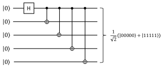
(a) The circuit to generate GHZ state $\frac{1}{\sqrt{2}}(\left|00000\right>+\left|11111\right>)$

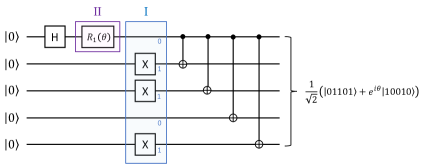
(b) The circuit to generate state $\frac{1}{\sqrt{2}}(\left|01101\right>+e^{i\theta}\left|10010\right>)$. It is obtained by inserting several proper X gates (step I) and an $R_{1}(\theta)$ gate (step II) in the circuit of (a).

Figure 18. Two quantum circuit examples of generating complementary superposition states.

Input: $n$-bit integer $x$ and the phase angle $\theta$.

Output: $n$-qubit state $\frac{1}{\sqrt{2}}(\left|x\right>+e^{i\theta}\left|\bar{x}\right>)$.

1

2if $x[0]=0$ then

3      $x^{\prime}\leftarrow x$;

4 else

5      $x^{\prime}\leftarrow\bar{x}$;

6 end if

7qs $\leftarrow\left|0\right>^{\otimes n}$; H(qs$[0]$);

8 $R_{1}$($\theta$, qs$[0]$);

9 for $i$ in $1\dots n-1$ do

10       if $x^{\prime}[i]=1$ then

11            X(qs$[i]$);

12       end if

13      CNOT(qs$[0]$, qs$[i]$);

14      

15 end for

16return qs;

Algorithm 3 Generate_KetX_plus_EITheta_KetNegX

A.3. Two Value Superposition States

This section outlines a generation algorithm for general two-value superposition states $\frac{1}{\sqrt{2}}(\left|x\right>+e^{i\theta}\left|y\right>)$. The process begins by comparing the binary representations of $x$ and $y$ and identifying the same and different bits, naturally dividing them into two groups. For the same bits, we apply Algorithm 2 to the corresponding qubits. For the different bits, we use Algorithm 3, incorporating a phase $e^{i\theta}$ on the corresponding qubits. The overall generation process is presented in Algorithm 4. To streamline the algorithm, we denote the sub-array of an original array Arr from the index set A as Arr[A].

Input: Two $n$-bit integers $x$ and $y$; phase angle $\theta$.

Output: $n$-qubit quantum state $\frac{1}{\sqrt{2}}(\left|x\right>+e^{i\theta}\left|y\right>)$.

1

2qs $\leftarrow\left|0\right>^{\otimes n}$;

3 $S\leftarrow$ the indexes of same bits of $x$ and $y$;

4 $D\leftarrow$ the indexes of different bits of $x$ and $y$;

5 $s\leftarrow x[S]$; $d\leftarrow x[D]$;

6 qs$[S]\leftarrow$ Generate_KetX($|S|$, $s$);

7 qs$[D]\leftarrow$ Generate_KetX_plus_EITheta_KetNegX($|D|$, $d$, $\theta$);

8 return qs;

Algorithm 4 Generate_KetX_plus_EITheta_KetY

A.4. Pauli States

As Formula (6) shows, multi-qubit Pauli states are represented as tensor products of several single-qubit Pauli states. There are six single-qubit Pauli states, as shown in the following:

• $\left|\Phi_{1}\right>=\left|0\right>$;

• $\left|\Phi_{2}\right>=\left|1\right>$;

• $\left|\Phi_{3}\right>=\left|+\right>=\frac{1}{\sqrt{2}}(\left|0\right>+\left|1\right>)$;

• $\left|\Phi_{4}\right>=\left|-\right>=\frac{1}{\sqrt{2}}(\left|0\right>-\left|1\right>)$;

• $\left|\Phi_{5}\right>=\left|+_{i}\right>=\frac{1}{\sqrt{2}}(\left|0\right>+i\left|1\right>)$;

• $\left|\Phi_{6}\right>=\left|-_{i}\right>=\frac{1}{\sqrt{2}}(\left|0\right>-i\left|1\right>)$.

To represent a single Pauli state, we use an integer $i$ ranging from 1 to 6, where each integer corresponds to a unique state $\left|\Phi_{i}\right>$. An $n$-qubit Pauli state can then be represented as an integer array with $n$ elements. The process to generate a single Pauli state $\left|\Phi_{i}\right>$ is described in Algorithm 5. To generate a multi-qubit Pauli state from a given integer array $A$, Algorithm 6 can be used.

Input: The index $i$ of single Pauli state.

Output: Single qubit Pauli state $\left|\Phi_{i}\right>$

1

2q $\leftarrow\left|0\right>$;

3 switch the value of $i$ do

4       case $i=2$ do X(q);

5        case $i=3$ do H(q);

6        case $i=4$ do X(q); H(q);

7        case $i=5$ do H(q); S(q);

8        case $i=6$ do H(q); S^†(q);

9       

10 end switch

11return q;

Algorithm 5 Generate_Single_Pauli

Input: The number of qubits $n$; the array $A$ of Pauli indexes (with length $n$).

Output: Pauli state associated with $A$.

1

2qs $\leftarrow\left|0\right>^{\otimes n}$;

3 for $i$ in $0\dots n-1$ do

4      qs$[i]\leftarrow$ Generate_Single_Pauli($A[i]$);

5 end for

6return qs;

Algorithm 6 Generate_Pauli_State

A.5. Mixed State

If we know the ensemble representation ${(p_{i},\left|\psi_{i}\right>)}$ of the target state $\rho$, and also the generate operation $U_{i}$ for each element state $\left|\psi_{i}\right>$, i.e., $U_{i}\left|0\right>=\left|\psi_{i}\right>$, we can use Algorithm 7 to execute $U_{i}$ with probability $p_{i}$ on $\left|0\right>$, which generates $\rho$ in the statistical sense. The output state of a single execution of Algorithm 7 is one of the states $\left|\psi_{i}\right>$, but the statistical distribution of multiple executions of the algorithm yields the ensemble ${(p_{i},\left|\psi_{i}\right>)}$, which represents the mixed state $\rho$.

Another scenario is when we only have access to the density matrix of $\rho$. In such cases, we can utilize spectrum decomposition to identify an ensemble representation (nielsen2002quantum, ), which is given by $\rho=\sum_{i}{\lambda_{i}}\left|i\right>\left<i\right|$. Assuming that we can identify the generation operation $U_{i}$ for each state $\left|i\right>$, Algorithm 7 can operate on this ensemble to generate the mixed state $\rho$.

Input: The ensemble representation $\{(p_{i},\left|\psi_{i}\right>)\}$ and the generate operation $U_{i}$ for each element state $\left|\psi_{i}\right>$.

Output: Target mixed state.

1 $r\leftarrow$ Random integer with probability distribution {$Pr[X=i]=p_{i}$};

2 qs = $\left|0\right>$; $U_{r}$(qs);

3 return qs;

Algorithm 7 Generate_Mixed_State

References

- (1) Abhari, A. J., Faruque, A., Dousti, M. J., Svec, L., Catu, O., Chakrabati, A., Chiang, C.-F., Vanderwilt, S., Black, J., and Chong, F. Scaffold: Quantum programming language. Tech. rep., Department of Computer Science, Princeton University, 2012.
- (2) Abreu, R., Fernandes, J. P., Llana, L., and Tavares, G. Metamorphic testing of oracle quantum programs. In 2022 IEEE/ACM 3rd International Workshop on Quantum Software Engineering (Q-SE) (2022), IEEE, pp. 16–23.
- (3) Aleksandrowicz, G., Alexander, T., Barkoutsos, P., Bello, L., Ben-Haim, Y., Bucher, D., Cabrera-Hernández, F. J., Carballo-Franquis, J., Chen, A., Chen, C.-F., Chow, J. M., Córcoles-Gonzales, A. D., Cross, A. J., Cross, A., Cruz-Benito, J., Culver, C., González, S. D. L. P., Torre, E. D. L., Ding, D., Dumitrescu, E., Duran, I., Eendebak, P., Everitt, M., Sertage, I. F., Frisch, A., Fuhrer, A., Gambetta, J., Gago, B. G., Gomez-Mosquera, J., Greenberg, D., Hamamura, I., Havlicek, V., Hellmers, J., Łukasz Herok, Horii, H., Hu, S., Imamichi, T., Itoko, T., Javadi-Abhari, A., Kanazawa, N., Karazeev, A., Krsulich, K., Liu, P., Luh, Y., Maeng, Y., Marques, M., Martín-Fernández, F. J., McClure, D. T., McKay, D., Meesala, S., Mezzacapo, A., Moll, N., Rodríguez, D. M., Nannicini, G., Nation, P., Ollitrault, P., O’Riordan, L. J., Paik, H., Pérez, J., Phan, A., Pistoia, M., Prutyanov, V., Reuter, M., Rice, J., Davila, A. R., Rudy, R. H. P., Ryu, M., Sathaye, N., Schnabel, C., Schoute, E., Setia, K., Shi, Y., Silva, A., Siraichi, Y., Sivarajah, S., Smolin, J. A., Soeken, M., Takahashi, H., Tavernelli, I., Taylor, C., Taylour, P., Trabing, K., Treinish, M., Turner, W., Vogt-Lee, D., Vuillot, C., Wildstrom, J. A., Wilson, J., Winston, E., Wood, C., Wood, S., Wörner, S., Akhalwaya, I. Y., and Zoufal, C. Qiskit: An Open-source Framework for Quantum Computing.
- (4) Ali, S., Arcaini, P., Wang, X., and Yue, T. Assessing the effectiveness of input and output coverage criteria for testing quantum programs. In 2021 14th IEEE Conference on Software Testing, Verification and Validation (ICST) (2021), IEEE, pp. 13–23.
- (5) Ammann, P., and Offutt, J. Using formal methods to derive test frames in category-partition testing. In Proceedings of COMPASS’94-1994 IEEE 9th Annual Conference on Computer Assurance (1994), IEEE, pp. 69–79.
- (6) Ammann, P., and Offutt, J. Introduction to software testing. Cambridge University Press, 2016.
- (7) Arora, S., and Barak, B. Computational complexity: a modern approach. Cambridge University Press, 2009.
- (8) Barenco, A., Berthiaume, A., Deutsch, D., Ekert, A., Jozsa, R., and Macchiavello, C. Stabilization of quantum computations by symmetrization. SIAM Journal on Computing 26, 5 (1997), 1541–1557.
- (9) Barnett, S. M., and Croke, S. Quantum state discrimination. arXiv preprint arXiv:0810.1970v1 (2008).
- (10) Beck, K. Test-driven development: by example. Addison-Wesley Professional, 2003.
- (11) Benedetti, M., Lloyd, E., Sack, S., and Fiorentini, M. Parameterized quantum circuits as machine learning models. Quantum Science and Technology 4, 4 (nov 2019), 043001.
- (12) Bichsel, B., Baader, M., Gehr, T., and Vechev, M. Silq: A high-level quantum language with safe uncomputation and intuitive semantics. In Proceedings of the 41st ACM SIGPLAN Conference on Programming Language Design and Implementation (2020), pp. 286–300.
- (13) Boyer, M., Brassard, G., H?yer, P., and Tapp, A. Tight bounds on quantum searching. Tech. rep., 1996.
- (14) Buhrman, H., Cleve, R., Watrous, J., and De Wolf, R. Quantum fingerprinting. Physical Review Letters 87, 16 (2001), 167902.
- (15) Burroughs, K., Jain, A., and Erickson, R. L. Improved quality of protocol testing through techniques of experimental design. In Proceedings of ICC/SUPERCOMM’94-1994 International Conference on Communications (1994), IEEE, pp. 745–752.
- (16) Cai, T., Kim, D., Wang, Y., Yuan, M., and Zhou, H. H. Optimal large-scale quantum state tomography with pauli measurements.
- (17) Cerezo, M., Poremba, A., Cincio, L., and Coles, P. J. Variational quantum fidelity estimation. Quantum 4 (2020), 248.
- (18) Chuang, I. L., and Nielsen, M. A. Prescription for experimental determination of the dynamics of a quantum black box. Journal of Modern Optics 44, 11-12 (1997), 2455–2467.
- (19) Cohen, D. M., Dalal, S. R., Fredman, M. L., and Patton, G. C. The aetg system: An approach to testing based on combinatorial design. IEEE Transactions on Software Engineering 23, 7 (1997), 437–444.
- (20) Cohen, D. M., Dalal, S. R., Kajla, A., and Patton, G. C. The automatic efficient test generator (aetg) system. In Proceedings of 1994 IEEE International Symposium on Software Reliability Engineering (1994), IEEE, pp. 303–309.
- (21) Córcoles, A. D., Takita, M., Inoue, K., Lekuch, S., Minev, Z. K., Chow, J. M., and Gambetta, J. M. Exploiting dynamic quantum circuits in a quantum algorithm with superconducting qubits. Phys. Rev. Lett. 127 (Aug 2021), 100501.
- (22) Dahl, O.-J., Dijkstra, E. W., and Hoare, C. A. R. Structured programming. Academic Press Ltd., 1972.
- (23) Deutsch, D. Quantum theory, the church–turing principle and the universal quantum computer. Proceedings of the Royal Society of London. A. Mathematical and Physical Sciences 400, 1818 (1985), 97–117.
- (24) Ekert, A. K., Alves, C. M., Oi, D. K., Horodecki, M., Horodecki, P., and Kwek, L. C. Direct estimations of linear and nonlinear functionals of a quantum state. Physical review letters 88, 21 (2002), 217901.
- (25) Flammia, S. T., and Liu, Y.-K. Direct fidelity estimation from few pauli measurements. Phys. Rev. Lett. 106 (Jun 2011), 230501.
- (26) Fortunato, D., Campos, J., and Abreu, R. Mutation testing of quantum programs: A case study with qiskit. IEEE Transactions on Quantum Engineering 3 (2022), 1–17.
- (27) Fortunato, D., Campos, J., and Abreu, R. Qmutpy: a mutation testing tool for quantum algorithms and applications in qiskit. In Proceedings of the 31st ACM SIGSOFT International Symposium on Software Testing and Analysis (2022), pp. 797–800.
- (28) García de la Barrera, A., García-Rodríguez de Guzmán, I., Polo, M., and Piattini, M. Quantum software testing: State of the art. Journal of Software: Evolution and Process (2021), e2419.
- (29) Google AI Quantum Team. Cirq.
- (30) Green, A. S., Lumsdaine, P. L., Ross, N. J., Selinger, P., and Valiron, B. An introduction to quantum programming in Quipper. In International Conference on Reversible Computation (2013), Springer, pp. 110–124.
- (31) Gross, D., Liu, Y.-K., Flammia, S. T., Becker, S., and Eisert, J. Quantum state tomography via compressed sensing. Physical review letters 105, 15 (2010), 150401.
- (32) Grover, L., and Rudolph, T. Creating superpositions that correspond to efficiently integrable probability distributions. arXiv preprint arXiv:quant-ph/0208112 (2002).
- (33) Grover, L. K. A fast quantum mechanical algorithm for database search. In Proceedings of the twenty-eighth annual ACM symposium on Theory of computing (1996), pp. 212–219.
- (34) Guo, J., Lou, H., Yu, J., Li, R., Fang, W., Liu, J., Long, P., Ying, S., and Ying, M. isq: An integrated software stack for quantum programming. IEEE Transactions on Quantum Engineering (2023), 1–18.
- (35) Harrow, A. W., Hassidim, A., and Lloyd, S. Quantum algorithm for linear systems of equations. Physical review letters 103, 15 (2009), 150502.
- (36) Honarvar, S., Mousavi, M., and Nagarajan, R. Property-based testing of quantum programs in Q#. In First International Workshop on Quantum Software Engineering (Q-SE 2020) (2020).
- (37) Hua, F., Jin, Y., Chen, Y., Vittal, S., Krsulich, K., Bishop, L. S., Lapeyre, J., Javadi-Abhari, A., and Zhang, E. Z. Caqr: A compiler-assisted approach for qubit reuse through dynamic circuit. In Proceedings of the 28th ACM International Conference on Architectural Support for Programming Languages and Operating Systems, Volume 3 (New York, NY, USA, 2023), ASPLOS 2023, Association for Computing Machinery, p. 59–71.
- (38) Huang, Y., and Martonosi, M. Statistical assertions for validating patterns and finding bugs in quantum programs. In Proceedings of the 46th International Symposium on Computer Architecture (2019), pp. 541–553.
- (39) Jose Campos, J., and Souto, A. Qbugs: A collection of reproducible bugs in quantum algorithms and a supporting infrastructure to enable controlled quantum software testing and debugging experiments. In Second International Workshop on Quantum Software Engineering (Q-SE 2021) (2021), pp. 28–32.
- (40) Knill, E. Approximation by quantum circuits, 1995.
- (41) Li, G., Zhou, L., Yu, N., Ding, Y., Ying, M., and Xie, Y. Projection-based runtime assertions for testing and debugging quantum programs. Proceedings of the ACM on Programming Languages 4, OOPSLA (2020), 1–29.
- (42) Liu, J., Byrd, G. T., and Zhou, H. Quantum circuits for dynamic runtime assertions in quantum computation. In Proceedings of the Twenty-Fifth International Conference on Architectural Support for Programming Languages and Operating Systems (2020), pp. 1017–1030.
- (43) Liu, J., and Zhou, H. Systematic approaches for precise and approximate quantum state runtime assertion. In IEEE International Symposium on High-Performance Computer Architecture, HPCA 2021, Seoul, South Korea, February 27 - March 3, 2021 (2021), IEEE, pp. 179–193.
- (44) Mendiluze, E., Ali, S., Arcaini, P., and Yue, T. Muskit: A mutation analysis tool for quantum software testing. In 2021 36th IEEE/ACM International Conference on Automated Software Engineering (ASE) (2021), IEEE, pp. 1266–1270.
- (45) Mingsheng, Y. Foundations of Quantum Programming, 1st ed. Morgan Kaufmann Publishers Inc., San Francisco, CA, USA, 2016.
- (46) Miranskyy, A., and Zhang, L. On testing quantum programs. In 2019 IEEE/ACM 41st International Conference on Software Engineering: New Ideas and Emerging Results (ICSE-NIER) (2019), IEEE, pp. 57–60.
- (47) Miranskyy, A., Zhang, L., and Doliskani, J. Is your quantum program bug-free? In 2020 IEEE/ACM 42nd International Conference on Software Engineering: New Ideas and Emerging Results (ICSE-NIER) (2020), IEEE Computer Society, pp. 29–32.
- (48) Miranskyy, A., Zhang, L., and Doliskani, J. On testing and debugging quantum software. arXiv preprint arXiv:2103.09172 (2021).
- (49) National Academies of Sciences, E., Medicine, et al. Quantum computing: progress and prospects. National Academies Press, 2019.
- (50) Nielsen, M. A., and Chuang, I. L. Quantum Computation and Quantum Information: 10th Anniversary Edition. Cambridge University Press, 2010.
- (51) Pérez-Delgado, C. A., and Pérez-González, H. G. Towards a quantum software modeling language. In First International Workshop on Quantum Software Engineering (Q-SE 2020) (2020).
- (52) Shor, P. W. Polynomial-time algorithms for prime factorization and discrete logarithms on a quantum computer. SIAM review 41, 2 (1999), 303–332.
- (53) Svore, K., Geller, A., Troyer, M., Azariah, J., Granade, C., Heim, B., Kliuchnikov, V., Mykhailova, M., Paz, A., and Roetteler, M. Q#: enabling scalable quantum computing and development with a high-level DSL. In Proceedings of the Real World Domain Specific Languages Workshop 2018 (2018), pp. 1–10.
- (54) Vogel, K., and Risken, H. Determination of quasiprobability distributions in terms of probability distributions for the rotated quadrature phase. Phys. Rev. A 40 (Sep 1989), 2847–2849.
- (55) Wang, J., Gao, M., Jiang, Y., Lou, J., Gao, Y., Zhang, D., and Sun, J. Quanfuzz: Fuzz testing of quantum program. arXiv preprint arXiv:1810.10310 (2018).
- (56) Wang, J., Zhang, Q., Xu, G. H., and Kim, M. Qdiff: Differential testing of quantum software stacks. ASE.
- (57) Wang, X., Arcaini, P., Yue, T., and Ali, S. Application of combinatorial testing to quantum programs. In 2021 IEEE 21st International Conference on Software Quality, Reliability and Security (QRS) (2021), IEEE, pp. 179–188.
- (58) Wang, X., Arcaini, P., Yue, T., and Ali, S. Generating failing test suites for quantum programs with search. In International Symposium on Search Based Software Engineering (2021), Springer, pp. 9–25.
- (59) Wang, X., Yu, T., Arcaini, P., Yue, T., and Ali, S. Mutation-based test generation for quantum programs with multi-objective search. In Proceedings of the Genetic and Evolutionary Computation Conference (2022), pp. 1345–1353.
- (60) Zhang, C., Feng, Y., and Ying, M. Unambiguous discrimination of mixed quantum states. Physics Letters A 353, 4 (2006), 300–306.
- (61) Zhang, C., Wang, G., and Ying, M. Discrimination between pure states and mixed states. Phys. Rev. A 75 (Jun 2007), 062306.
- (62) Zhao, J. Quantum software engineering: Landscapes and horizons. arXiv preprint arXiv:2007.07047 (2020).
- (63) Zhao, P., Zhao, J., Miao, Z., and Lan, S. Bugs4q: A benchmark of real bugs for quantum programs. In 2021 36th IEEE/ACM International Conference on Automated Software Engineering (ASE) (2021), IEEE, pp. 1373–1376.