Modeling the $R$-ratio and hadronic contributions to $g-2$ with a Treed Gaussian Process

Andrew Fowlie
Department of Physics, School of Mathematics and Physics, Xi’an Jiaotong-Liverpool University, Suzhou 215123, China
Qiao Li
Department of Physics and Institute of Theoretical Physics, Nanjing
Normal University, Nanjing, Jiangsu 210023, China

The BNL and FNAL measurements of the anomalous magnetic moment of the muon disagree with the Standard Model (SM) prediction by more than $4\sigma$. The hadronic vacuum polarization (HVP) contributions are the dominant source of uncertainty in the SM prediction. There are, however, tensions between different estimates of the HVP contributions, including data-driven estimates based on measurements of the $R$-ratio. To investigate that tension, we modeled the unknown $R$-ratio as a function of CM energy with a treed Gaussian process (TGP). This is a principled and general method grounded in data-science that allows complete uncertainty quantification and automatically balances over- and under-fitting to noisy data. Our tool yields exploratory results are similar to previous ones and we find no indication that the $R$-ratio was previously mismodeled. Whilst we advance some aspects of modeling the $R$-ratio and develop new tools for doing so, a competitive estimate of the HVP contributions requires domain-specific expertise and a carefully curated database of measurements.

1  Introduction

The final measurement of the anomalous magnetic moment of the muon at the Brookhaven National Laboratory (BNL) E821 experiment [1] differed from the Standard Model (SM) prediction by $3.7\sigma$. This discrepancy was replicated by the Fermi National Accelerator Laboratory (FNAL) E989 measurement [2]. The combined measurement from BNL and FNAL,

$$a_{\mu}=116\,592\,061\,(41)\times 10^{-11},$$ (1)

deviates from the SM theory prediction by $4.2\sigma$, motivating the possibility of physics beyond the SM [3] as well as scrutiny of the SM prediction [4].

The SM prediction for $a_{\mu}$ incorporates contributions from quantum electrodynamics (QED), electroweak interactions (EW), and hadronic effects [5]. While QED and EW contributions can be calculated with high precision using perturbation theory and are well-controlled [6], hadronic contributions are harder to compute and are the largest source of uncertainty in predictions for $a_{\mu}$. The hadronic contribution can itself be decomposed into the following parts:

$$a_{\mu}^{\mathrm{had}} =a_{\mu}^{\textsc{hvp}}+a_{\mu}^{\mathrm{LbL}},$$ (2)

where $a_{\mu}^{\textsc{hvp}}$ is the hadronic vacuum polarization (HVP) contribution and $a_{\mu}^{\mathrm{LbL}}$ is the light-by-light scattering contribution. In this work we focus on the leading-order (LO) contribution to HVP. This is particularly challenging and the dominant source of uncertainty, making up about $80\%$ of the total. The two most popular computational methods are lattice QCD and estimates from dispersion integrals and cross-section data.

Lattice methods calculate the HVP contribution by discretizing spacetime and performing a weighted integral of relevant functions over Euclidean time. This requires significant computational resources and currently cannot match the nominal precision achieved by data-driven methods. Data-driven methods use data from, for example, the KLOE [7], BaBar [8, 9, 10, 11], SND [12] and CMD-3 [13, 14] experiments to estimate the $R$-ratio,

$$R(s)\equiv\frac{\sigma^{0}(e^{+}e^{-}\to\text{hadrons})}{\sigma(e^{+}e^{-}\to\mu^{+}\mu^{-})}.$$ (3)

This is a function of the center-of-mass (CM) energy, $\sqrt{s}$. From the estimate of the $R$-ratio, the leading-order (LO) HVP contributions can be computed through the dispersion integral,

$$a_{\mu}^{\textsc{hvp}}=\frac{\alpha^{2}}{3\pi^{2}}\int\limits_{m_{\pi}^{2}}^{\infty}\frac{K(s)R(s)}{s}\,\text{d}s$$ (4)

where $K(s)$ is the QED kernel [15, 16]. Hadronic contributions to the effective electromagnetic coupling constant at the $Z$ boson mass can be computed in a similar way through the dispersion relationship

$$\Delta\alpha_{\text{had}}=\frac{\alpha M_{Z}^{2}}{3\pi}\fint\limits_{m_{\pi}^{2}}^{\infty}\frac{R(s)}{s(M_{Z}^{2}-s)}\text{d}s$$ (5)

where $\fint$ represents the principal-value prescription. There is growing tension between results from the two approaches [17, 18]. A recent lattice QCD calculation found [19]

$$a_{\mu}^{\textsc{hvp}}=707.5\,(5.5)\times 10^{-10}$$ (6)

whereas a conservative combination of data-driven estimates yielded [4]

$$a_{\mu}^{\textsc{hvp}}=693.1\,(4.0)\times 10^{-10}.$$ (7)

The lattice result was at least partly corroborated by other recent lattice computations [20, 21, 22] and, moreover, data-driven estimates using hadronic $\tau$-decays are close to lattice results [23]. The most recent measurement of the $2\pi$ final state at CDM-3 [24] compounded the mystery, as it conflicts with older measurements including CDM-2 [25].

With these issues in mind, we wish to reconsider the statistical methodology for inferring the $R$-ratio from noisy data. As we shall discuss in section 2, the existing approaches use carefully constructed but ad hoc techniques and closed-source software, and consider uncertainties in a frequentist framework. The data-driven approach, though, is connected to common problems in data-science and statistics: modeling an unknown function (here the $R$-ratio) and managing the risks of under- and over-fitting. In section 3, we describe how we tackle these issues using Gaussian processes — flexible non-parametric statistical models — and marginalization of the model’s hyperparameters. This allows coherent uncertainty quantification and regularizes the wiggliness of the $R$-ratio, which helps prevent the model from over-fitting the noisy data. Our algorithm is implemented in our public kingpin package documented in a separate paper [28]. We focus on modeling choices and developing a tool for principled modeling of the $R$-ratio; our estimates are supplementary to existing ones and we don’t attempt to match previous comprehensive estimates in all respects. We don’t anticipate dramatic differences with respect to previous findings; however, careful modeling of the $R$-ratio is important because $\mathcal{O}(1\%)$ changes in the HVP contribution or finding that the uncertainty was underestimated could resolve tension with the experimental measurements and lattice predictions. We present predictions from our model for $a_{\mu}^{\textsc{hvp}}$ and $\Delta\alpha_{\text{had}}$ in section 4. Finally, we conclude in section 5.

2  Existing data-driven methods

We now briefly review two data-driven methods for calculating $a_{\mu}^{\textsc{hvp}}$. First, the DHMZ approach [29, 30, 31], which employs HVPTools, a private software package that combines and integrates cross-section data from $e^{+}e^{-}\to\text{hadrons}$. For each experiment, second-order polynomial interpolation is used between adjacent measurements to discretize the results into small bins (of around $1\,\text{MeV}$) for later averaging and numerical integration. The HVP contributions are estimated in a frequentist framework. To ensure that uncertainties are propagated consistently, pseudo-experiments are generated and closure tests with known distributions are performed to validate the data combination and integration. If the results from different experiments are locally inconsistent, the uncertainty of the combination is readjusted according to the local $\chi^{2}$ value following the well-known PDG approach [32].

The second method is the KNT approach [4, 33, 34], which performs a data-driven compilation of hadronic $R$-ratio data to calculate the HVP contribution. It first selects the data to be used and then bins the data using a clustering procedure to avoid over-fitting. The clustering procedure determines the optimal binning of data for all channels into a set of clusters based on the available local data density. The optimal clustering criteria are shown in Ref. [4]. As of Ref. [33], the KNT compilation uses an iterated $\chi^{2}$ fit to achieve the actual combination. This new method ensures that the covariance matrix is re-initialized at each iteration. The motivation of this procedure is to avoid bias. The fit results in the mean $R$-ratio for each cluster and a full covariance matrix containing all correlated and uncorrelated uncertainties. Combined with trapezoidal integration, these are used to determine channel-by-channel contributions to $a_{\mu}^{\textsc{hvp}}$.

The DHMZ and KNT approaches are both data-driven methods that estimate $a_{\mu}^{\textsc{hvp}}$ in a frequentist framework, using privately curated databases of measurements, and in-house custom codes and techniques to avoid over-fitting. The differences between the two methods are not only evident in their distinct compilation targets — the DHMZ approach combines and integrates cross-section data from $e^{+}e^{-}\to\text{hadrons}$, while the KNT approach performs a data-driven compilation of the hadronic $R$-ratio. Furthermore, discernible disparities emerge in their respective data handling procedures, encompassing data selection, data combination, and the propagation of uncertainties. Each method has its own strengths and limitations. While DHMZ and KNT approaches do not exhibit significant differences in estimating the central value of $a_{\mu}^{\textsc{hvp}}$, there are significant disparities in the resulting uncertainties and the shapes of the combined spectra.

3  Treed Gaussian process

3.1  Gaussian processes

In our data-driven approach, we model the unknown $R$-ratio with Gaussian processes (GPs; [35, 36]). A GP generalizes the Gaussian distribution. Roughly speaking, whereas a Gaussian describes the distribution of a scalar and a multivariate Gaussian describes the distribution of a vector, a GP describes the distribution of a function — an infinite collection of variables $f(x)$ indexed by a location $x$. Any subset of the random variables are correlated through a multivariate Gaussian. The degree of correlation between $f(x)$ and $f(x^{\prime})$ governs the smoothness of $f(x)$ and is set by a choice of kernel function, $k(x,x^{\prime})$.

Just as a GP generalizes a Gaussian distribution of scalars or vectors to a distribution of functions, it allows us to generalize inference over unknown scalars or vectors to inference over unknown functions. Suppose we wish to learn an unknown function. Because a GP describes the distribution of a function, it can be used as the prior for the unknown function in a Bayesian setting. This prior distribution can be updated through Bayes’ rule by any noisy measurements or exact calculations of the values of $f$ at particular locations $x$. In this paper we will update a GP for the $R$-ratio by the noisy measurements of the $R$-ratio. We use celerite2 [37] for ordinary GP computations.

The kernel function is usually stationary, that is, depends only on the Euclidean distance between locations,

$$k(x,x^{\prime})=k(|x-x^{\prime}|).$$ (8)

Once a particular form of stationary kernel has been chosen, a GP can be controlled by three hyperparameters: a constant mean $\mu$,

$$\textsf{E}\mathopen{}\mathclose{{}\left[\vphantom{R_{i},R_{j}}f(x)}\right]=\mu,$$ (9)

and a scale $\sigma$ and length $\ell$ that govern the covariance,

$$\textsf{Cov}\mathopen{}\mathclose{{}\left[\vphantom{R_{i},R_{j}}f(x),f(x^{\prime})}\right]=\sigma^{2}k\left(\frac{|x-x^{\prime}|}{\ell}\right).$$ (10)

The scale controls the size of wiggles in the function predicted by the GP. The length determines the length scale over which correlation decays and hence the number of wiggles in an interval. For Gaussian kernels, by Rice’s formula [38] the expected number of wiggles per unit distance scales as $1/\ell$. These three hyperparameters can substantially affect how well a GP models an unknown function. In a fully Bayesian framework, the hyperparameters are marginalized. This automatically weights choices of hyperparameter by how well they model the data and alleviates overfitting. The wigglines is regularized and the fit needn’t pass through every data point.

3.2  Treed Gaussian processes

The GPs described thus far are stationary — they model all regions of input space identically. To allow for non-stationary structure in the $R$-ratio, we use a treed-GP (TGP; [39, 40]). This is necessary as we know that the $R$-ratio contains narrow features such as resonances. In a TGP, the input space is partitioned using a binary tree. The predictions in each partition are governed by a different GP with independent hyperparameters. The number and locations of partitions are modeled using the so-called CGM prior [41].

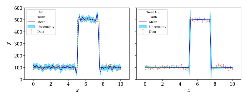
Figure 1: The GP (left) predicts a wiggly fit to the straight line sections due to the step. The TGP (right) automatically addresses the issue by partitioning the input space.

The difference in predictions between a GP and our TGP is illustrated in fig. 1. In this illustration we consider evenly spaced noisy measurements of a function that contains a step. The GP (left) models the data poorly, as to accommodate the sudden step, the covariance between input locations must be weak which results a wiggly fit to the straight-line sections. The TGP (right) automatically partitions the input space allowing it to model the distinct straight-line sections separately. At the jumps before and after the step, the TGP predicts the function with substantial uncertainty. This is satisfying since the data points change dramatically across those regions of input space and do not indicate what might happen inside them.

TGPs build on ideas such as CART [41], treed models generally [42] and partitioning [43], and are similar to piece-wise GPs [44] and a recent proposal in machine learning [45]. Alternative approaches to non-stationarity include non-stationary kernel functions [46], Deep GPs [47, 48] where non-stationarity is modeled through warping, and hierarchical models of GPs [49, 50]. There is valuable discussion and comparison of these approaches in Ref. [51, 52] and this remains an active area. As well as addressing non-stationarity in unknown functions, these approaches address heteroscedastic noise in our measurements.

Our approach is fully Bayesian — we marginalize the GP hyperparameters and tree structure. This decreases the risk of over- or under-fitting the noisy data and smooths the partitions between GPs. We perform marginalization numerically using reversible jump Markov Chain Monte Carlo (RJ-MCMC; [53]. For reviews see Ref. [54, 55, 56]). This is a generalization of MCMC that works on parameter spaces that don’t have a fixed dimension — this is vital because the number of GPs and thus the total number of hyperparameters isn’t fixed. Navigating the tree structure requires special RJ-MCMC proposals — such as growing, pruning and rotating the tree — that are described in Ref. [39].

3.3  Integration

The idea of modeling integrals through GPs was originally known by Bayes-Hermite quadrature [57], and later discussed under the names of Bayesian Monte Carlo (BMC; [58]) and Bayesian quadrature or cubature [59, 60]; see Ref. [61] for a review. Suppose we wish to compute an integral of the form,

$$I=\int C(x)f(x)\,\text{d}x$$ (11)

where $f(x)$ is the estimated function and $C(x)$ is a known function. BMC provides an epistemic meaning to errors in quadrature estimates of theses integrals, such as

$$I\approx\sum_{i}C(x)f(x_{i})\Delta x_{i},$$ (12)

because we may make inferences on $I$ through our statistical model for $f(x)$. In cases in which the function $C(x)$ and choice of kernel lead to intractable computations, there is an additional discretization error in BMC inferences as the GP predictions are evaluated on a finitely-spaced grid. This is known as approximate Bayesian cubature [61]. This additional error may be neglected when the integrand is approximately linear between prediction points. We will use a TGP to model an integrand. Although trees have been proposed in BMC [62], they haven’t previously been directly combined with GPs in this way.

3.4  Sequential design

After completing inference of an unknown function with the data at hand, one may wish to know what data to collect next. This problem is known as sequential design or active learning. Broadly speaking, this is a challenging question and greedy approaches that make optimal choices one step at a time are easier to implement. We thus consider a variant of Active Learning Mackay (ALM; [63, 64]).

Following the approach in Ref. [65], we consider the location that contributes most to the uncertainty in the $a_{\mu}^{\textsc{hvp}}$ and $\Delta\alpha_{\text{had}}$ integrals to be an optimal location at which to perform more measurements. For an integral of the form eq. 11, we compute

$$x_{\text{ALM}}=\operatorname*{arg\,max}\nolimits_{x}\left[\int C(x)\,\textsf{Cov}\mathopen{}\mathclose{{}\left[\vphantom{R_{i},R_{j}}f(x),f(y)}\right]\,C(y)\,\text{d}y\right].$$ (13)

See Ref. [66, 40] for further discussion.

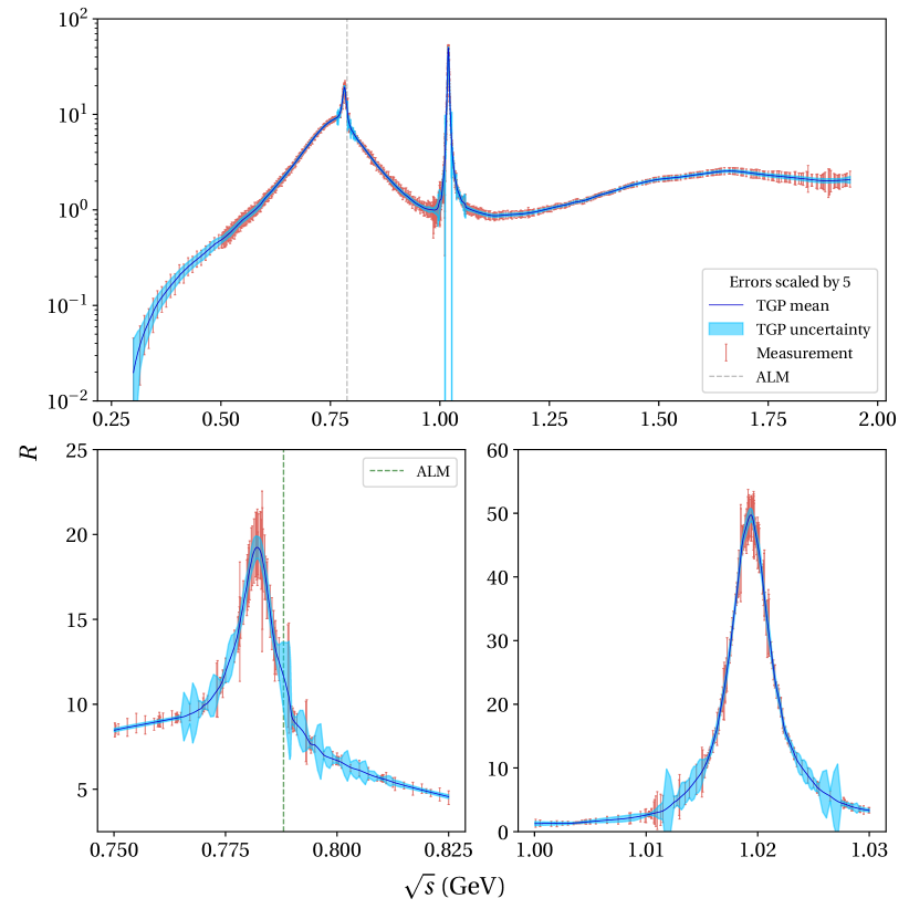
Figure 2: Predicted $R$-ratio from the TGP model. The experimental errors and uncertainty in the TGP predictions are scaled by $5$ and the $\rho$ – $\omega$ and $\phi$ resonances are plotted separately for visibility.

4  Results

4.1  Data selection

We investigated the public dataset from the Particle Data Group (PDG; [32, 67]. See also Ref. [68] for further details), which primarily comprises data on the inclusive $R$-ratio, asymmetric statistical errors, and point-to-point systematic errors from electron-positron annihilation to hadrons at different CM energies. Certain CM energies may have multiple point-to-point systematic uncertainties stemming from different sources. We symmetrized errors and combined systematic ($\tau$) and statistical errors ($\sigma$) in quadrature:

$$\tau^{2}=\sum_{i}\tau_{i}^{2} \quad\text{where}\quad\tau_{i}=\frac{1}{2}(\tau_{\text{up}}+\left|\tau_{\text{down}}\right|),$$ (14)

$$\sigma_{\text{total}}=\sqrt{\sigma^{2}+\tau^{2}} \quad\text{where}\quad\sigma=\frac{1}{2}(\sigma_{\text{up}}+\left|\sigma_{\text{down}}\right|).$$ (15)

We selected $859$ data points inside the CM energy interval $0.3$ – $1.937\,\text{GeV}$. This interval was selected to facilitate a comparison with Ref. [33]. The maximum $\sqrt{s}=1.937\,\text{GeV}$ was chosen as it is the point at which summing exclusive $R$-ratio data becomes unfeasible and perturbative QCD may be reliable. The minimum $\sqrt{s}=0.3\,\text{GeV}$ was the minimum energy in the public PDG dataset.

To model this data set, we utilized a treed Gaussian process (TGP), as described in section 3. Besides selecting the data, we must specify the locations at which we want to predict the $R$-ratio. In our study, we predicted at every input location and at two uniformly spaced locations between every pair of consecutive input locations.

4.2  Computational methods and modelling choices

We model the $R$-ratio by a TGP in which the input space is divided into partitions using a binary tree. Each partition in our TGP is governed by a mean, $\mu$, and a Matérn-3/2 kernel with independent scale, $\sigma$, and length, $\ell$, hyperparameters. We use a uniform prior between $0$ and $150$ for the mean, a uniform prior between $0$ and $500$ for the scale, and a uniform prior between $0\,\text{GeV}$ to $5\,\text{GeV}$ for the length. These choices were motivated by the maximum measured $R$-ratio and the CM interval $0.3$ – $1.937\,\text{GeV}$ under consideration. Following Ref. [39], the structure of the tree itself is controlled by a CGM prior with hyperparameters $\alpha=0.5$ and $\beta=2$; see Ref. [41] for explanation of these parameters. These choices favor smaller and more balanced trees.

We marginalize the tree structure and hyperparamters using RJ-MCMC. To improve computational efficiency, we thin the chains by a factor of four and only compute predictions for the states in the thinned chains. This reduces the computational time but only slightly reduces the effective sample size as the states in the unthinned chain are strongly correlated. We run RJ-MCMC for 300 000 steps but discard 5000 burn-in steps to minimize bias from the beginning of the chain. For computational efficiency and following a multistart heuristic, we run 10 chains in parallel and combine them.

4.3  Predictions

The predictions from our TGP model for the $R$-ratio are shown in fig. 2 as a mean and an error band. The mean predictions pass smoothly around the data points without any undue fluctuations near the data points that are characteristic of over-fitting. The $\rho$ – $\omega$ and $\phi$ resonances are typically fitted by their own tree partitions with separate hyperparameters. They aren’t forced to be as smooth as the rest of the spectrum and appear well-fitted. Our model predictions are noticeably more uncertain in regions with fewer or noisy measurements. We identify no anomalous features and tentatively conclude that the RJ-MCMC marginalization adequately converged. We ran standard MCMC diagnostics on the mean of the $R$-ratio using ArviZ [69]; finding $n_{\text{eff}}\simeq 600$ bulk effective samples and Gelman-Rubin diagnostic $1.01$ [70]. There are typically five or six partitions, as the two peaks and the three flatter regions are modeled separately as shown in fig. 3. In fig. 4 we show the result when using an ordinary GP. To accommodate the narrow peaks in the measured $R$-ratio, the GP model permits substantial wiggles between data points, especially where the data points are sparse.

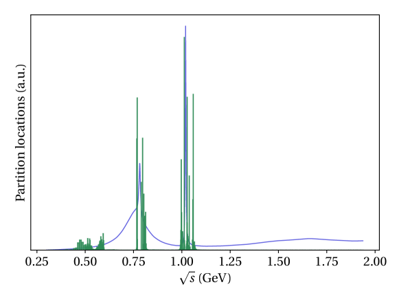
Figure 3: Histogram of locations of partition edges in the TGP model. The mean prediction for the $R$-ratio is shown for reference (blue).

The TGP model outputs the mean, $\textsf{E}\mathopen{}\mathclose{{}\left[\vphantom{R_{i},R_{j}}R_{i}}\right]$, and covariance, $\textsf{Cov}\mathopen{}\mathclose{{}\left[\vphantom{R_{i},R_{j}}R_{i},R_{j}}\right]$, of the $R$-ratio at the prediction locations $\sqrt{s}_{i}$. The mean function represents the expected or average output value for a given input value, while the covariance function represents the covariance between predictions at different CM energies. As the RJ-MCMC can be computationally expensive and time-consuming, we saved these results to disk and made them publicly available [71]. We used the mean and covariance predictions for $R$ in combination with the dispersion integrals to predict contributions to $a_{\mu}^{\textsc{hvp}}$ and $\Delta\alpha_{\text{had}}$ from the CM energy interval of $0.3$ – $1.937\,\text{GeV}$. As $a_{\mu}^{\textsc{hvp}}$ and $\Delta\alpha_{\text{had}}$ are linear functions of $R$, we propagate $\textsf{E}\mathopen{}\mathclose{{}\left[\vphantom{R_{i},R_{j}}R_{i}}\right]$ and $\textsf{Cov}\mathopen{}\mathclose{{}\left[\vphantom{R_{i},R_{j}}R_{i},R_{j}}\right]$ to obtain predictions. In all subsequent integration processes, we employ the trapezoidal rule [72], and in subsequent formulae $\sqrt{s}$ denotes the locations of our TGP predictions rather than the locations of the measurements.

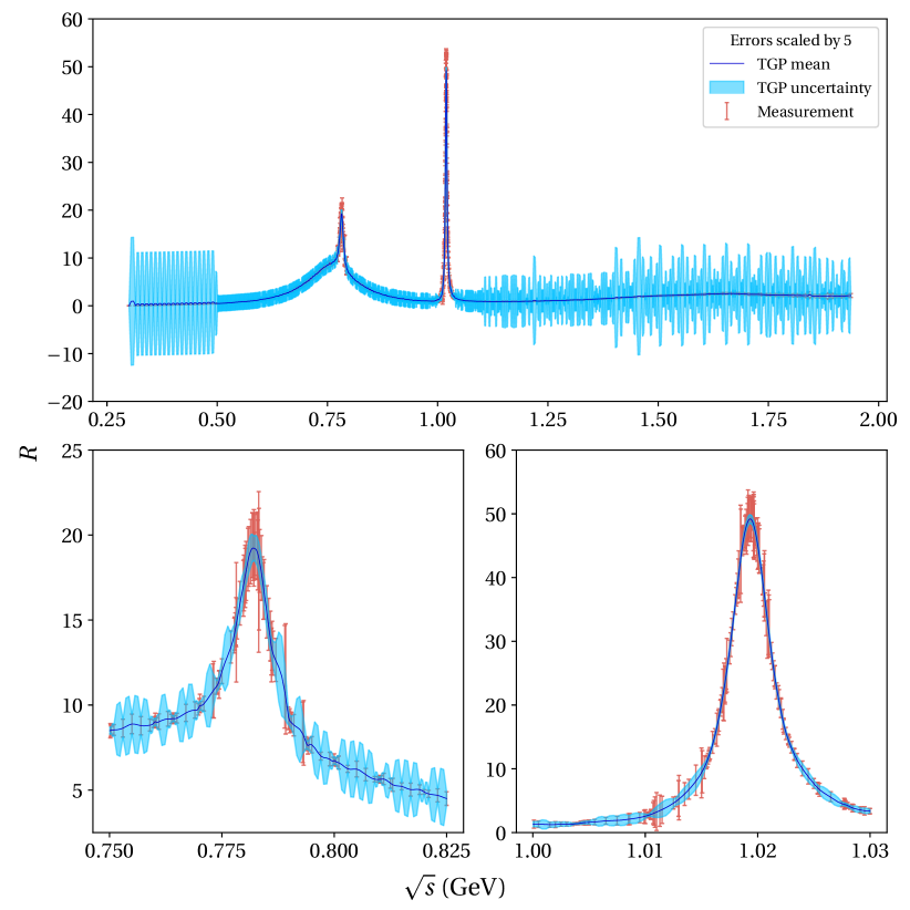
Figure 4: Similar to fig. 2, though showing results from an ordinary GP.

The calculation of $a_{\mu}^{\textsc{hvp}}$ is based on eq. 4. However, since the independent variable in this case is the CM energy, a simple deformation of eq. 4 is necessary,

$$a_{\mu}^{\textsc{hvp}}=\frac{2\alpha^{2}}{3\pi^{2}}\int_{m_{\pi}^{2}}^{\infty}\frac{K(s)R(\sqrt{s})}{\sqrt{s}}\,\text{d}\sqrt{s}$$ (16)

Then we calculate the value of $a_{\mu}^{\textsc{hvp}}$ through numerical quadrature,

$$a_{\mu}^{\textsc{hvp}}=\sum_{i}C^{\textsc{hvp}}_{i}R_{i}$$ (17)

where we defined

$$C^{\textsc{hvp}}_{i}\equiv\frac{2\alpha^{2}}{3\pi^{2}}\frac{K(\sqrt{s}_{i})}{\sqrt{s}_{i}}w_{i}$$ (18)

where $w_{i}$ are the quadrature weights. We use the trapezoid rule such that

$$w_{i}=\frac{1}{2}\begin{cases}\sqrt{s}_{2}-\sqrt{s}_{1}&i=1\\ \sqrt{s}_{N}-\sqrt{s}_{N-1}&i=N\\ \sqrt{s}_{i+1}-\sqrt{s}_{i-1}&\text{otherwise.}\end{cases}$$ (19)

From eq. 17 and by linearity, the mean can be found through

$$\textsf{E}\mathopen{}\mathclose{{}\left[\vphantom{R_{i},R_{j}}a_{\mu}^{\textsc{hvp}}}\right]=\sum_{i}C^{\textsc{hvp}}_{i}\textsf{E}\mathopen{}\mathclose{{}\left[\vphantom{R_{i},R_{j}}R_{i}}\right],$$ (20)

and from the covariance matrix for predictions of the $R$-ratio, the uncertainty in our prediction of $a_{\mu}^{\textsc{hvp}}$ can be calculated using

$$\textsf{Var}\mathopen{}\mathclose{{}\left[\vphantom{R_{i},R_{j}}a_{\mu}^{\textsc{hvp}}}\right]=\textsf{Var}\mathopen{}\mathclose{{}\left[\vphantom{R_{i},R_{j}}\sum_{i}C^{\textsc{hvp}}_{i}R_{i}}\right]=\sum_{i,j=1}^{n}C^{\textsc{hvp}}_{i}\,C^{\textsc{hvp}}_{j}\,\textsf{Cov}\mathopen{}\mathclose{{}\left[\vphantom{R_{i},R_{j}}R_{i},R_{j}}\right].$$ (21)

We compute $\Delta\alpha_{\text{had}}$ similarly using,

$$\Delta\alpha_{\text{had}}=\frac{2\alpha M_{Z}^{2}}{3\pi}\fint\limits_{m_{\pi}^{2}}^{\infty}\frac{R(\sqrt{s})}{\sqrt{s}(M_{Z}^{2}-(\sqrt{s})^{2})}\text{d}\sqrt{s}.$$ (22)

We use eqs. 20 and 21 though with coefficients,

$$C^{\text{had}}_{i}=\frac{2\alpha M_{Z}^{2}}{3\pi}\frac{w_{i}}{\sqrt{s}_{i}\left[M_{Z}^{2}-s_{i}\right]}.$$ (23)

Because our calculation is performed at CM energies from $0.3$ – $1.937\,\text{GeV}$, the principal-value prescription does not need to be considered.

For the sake of comparison and to verify parts of our tool-chain, we calculate $a_{\mu}^{\textsc{hvp}}$ and $\Delta\alpha_{\text{had}}$ naively without utilizing a TGP. We consider a naive model that at the locations of the measurements of the $R$-ratio predicts

$$R_{i}=\hat{R}_{i}\pm\sigma_{i}$$ (24)

where $\hat{R}_{i}$ are the central values and $\sigma_{i}$ are the errors of the measurements. In this naive model there is no covariance between predictions, that is, $\textsf{Cov}\mathopen{}\mathclose{{}\left[\vphantom{R_{i},R_{j}}R_{i},R_{j}}\right]=0$ for $i\neq j$. Equations 20 and 21 apply to this simple case, although it should be noted that in this case $\sqrt{s}$ are a series of data points, whereas in the TGP $\sqrt{s}$ are the chosen prediction locations.

The results of the above calculations are summarized in table 1. We show the predictions from KNT18 [33] and KNT19 [34] for comparison, which are found by summing data-based exclusive channels in tables 2 and 1, respectively, and combing errors in quadrature. We see that the TGP prediction for $a_{\mu}^{\textsc{hvp}}$ is smaller than predictions from the naive model, KNT18 [33] and KNT19 [34]. This would make tension between data-driven estimates and lattice QCD and the experimental measurements worse. The uncertainties in our TGP predictions are nearly identical to those from the naive model — we explain this similarity in uncertainties in appendix A — though substantially smaller than those from KNT18 [33] and KNT19 [34]. We don’t anticipate that the smaller TGP uncertainties are a consequence of the TGP model itself; rather, KNT18 [33] and KNT19 [34] are based on a different dataset and treatment of systematics. For example, they include uncertainties from vacuum polarization (VP) effects and final-state radiation (FSR) that we omit. We thus find no clear evidence of mismodelling or that our more careful modeling can shed light on the tension between data-driven estimates, lattice estimates and experiments. It is possible, however, that for an identical dataset to that in KNT18 [33] and KNT19 [34], the TGP predictions could be greater than KNT18 [33] and KNT19 [34]— the impact of reducing overfitting with a TGP could work in the opposite direction in that dataset.

	Treed GP Model	Naive Model	KNT18 [33]	KNT19 [34]
$a_{\mu}^{\textsc{hvp}}\times 10^{10}$	$636.34\pm 0.83$	$637.73\pm 0.84$	$638.59\pm 2.35$	$638.25\pm 2.32$
$\Delta\alpha_{\text{had}}\times 10^{4\phantom{0}}$	$57.28\pm 0.05$	$57.41\pm 0.05$	$57.83\pm 0.29$	$57.88\pm 0.29$

Table 1: Contributions to $a_{\mu}^{\textsc{hvp}}$ and $\Delta\alpha_{\text{had}}$ in the CM energy range of $0.3$ – $1.937\,\text{GeV}$ from our TGP model, a naive model, KNT18 [33] and KNT19 [34].

4.4  Sequential design

We may use our TGP result to identify locations that contribute most to the uncertainty in the $a_{\mu}^{\textsc{hvp}}$ and $\Delta\alpha_{\text{had}}$ predictions and where future measurements would be most beneficial. For both $a_{\mu}^{\textsc{hvp}}$ and $\Delta\alpha_{\text{had}}$, the ALM estimate from eq. 13 yields

$${\sqrt{s}}_{\text{ALM}}=0.788\,\text{GeV}.$$ (25)

This lies near noisy measurements after the $\rho$ – $\omega$ resonance; see fig. 2. Besides lying close to noisy measurements, the uncertainty at this location is substantial because it is a boundary between partitions of the TGP — the behavior of the function changes abruptly here and so is hard to predict.

4.5  Correlation

Lastly, let us consider the relationship between the predictions for $a_{\mu}^{\textsc{hvp}}$ and $\Delta\alpha_{\text{had}}$. From eqs. 4 and 5, we observe that the dispersion integral formulas used to calculate $a_{\mu}^{\textsc{hvp}}$ and $\Delta\alpha_{\text{had}}$ both involve the $R$-ratio. To quantify this relationship, covariance can be used to measure the correlation between two variables. The sign of covariance indicates whether the trends between the two variables are consistent. The correlation coefficient is usually utilized to reflect the strength of the correlation between two variables. Thus, to gain more understanding about the relationship between $a_{\mu}^{\textsc{hvp}}$ and $\Delta\alpha_{\text{had}}$, we computed their covariance and correlation,

$$\textsf{Cov}\mathopen{}\mathclose{{}\left[\vphantom{R_{i},R_{j}}a_{\mu}^{\textsc{hvp}},\Delta\alpha_{\text{had}}}\right] =\sum_{i,j=1}^{n}C^{\textsc{hvp}}_{i}\,C^{\text{had}}_{j}\,\textsf{Cov}\mathopen{}\mathclose{{}\left[\vphantom{R_{i},R_{j}}R_{i},R_{j}}\right]$$ (26)

$$\rho\mathopen{}\mathclose{{}\left[\vphantom{R_{i},R_{j}}a_{\mu}^{\textsc{hvp}},\Delta\alpha_{\text{had}}}\right] =\frac{\textsf{Cov}\mathopen{}\mathclose{{}\left[\vphantom{R_{i},R_{j}}a_{\mu}^{\textsc{hvp}},\Delta\alpha_{\text{had}}}\right]}{\sqrt{\textsf{Var}\mathopen{}\mathclose{{}\left[\vphantom{R_{i},R_{j}}a_{\mu}^{\textsc{hvp}}}\right]\textsf{Var}\mathopen{}\mathclose{{}\left[\vphantom{R_{i},R_{j}}\Delta\alpha_{\text{had}}}\right]}}$$ (27)

where the (co)variances were computed under the TGP as described. As anticipated, we obtained a positive correlation between the two. Specifically, when $\Delta\alpha_{\text{had}}$ increases, the value of $a_{\mu}^{\textsc{hvp}}$ also increases, and vice versa. The calculated correlation coefficient was $\rho\simeq 0.8$, which is close to $1$, quantifying the strong correlation between $a_{\mu}^{\textsc{hvp}}$ and $\Delta\alpha_{\text{had}}$.

5  Discussion and conclusions

The BNL and FNAL measurements of the anomalous magnetic moment of the muon disagree with the Standard Model (SM) prediction by more than $4\sigma$. This has led to renewed scrutiny of new physics explanations and the SM prediction. With that as motivation, we extracted the hadronic vacuum polarization (HVP) contributions, $a_{\mu}^{\textsc{hvp}}$, from electron cross-section data using a treed Gaussian process (TGP) to model the unknown $R$-ratio as a function of CM energy. This is a principled and general method from data-science, that allows complete uncertainty quantification and automatically balances over- and under-fitting to noisy data.

The challenges in the data-driven approach are common in data-science. A competitive estimate of $a_{\mu}^{\textsc{hvp}}$, however, requires domain-specific expertise, careful curation of measurements, and careful consideration of systematic errors and their correlation. This should be developed over time in collaboration with domain experts. Thus our work should be seen as preliminary and serves to explore an alternative statistical methodology based on more general principles and develop an associated toolchain. We used a dataset available from the PDG, though as noted as early as 2003 in Ref. [68], a more complete, documented and standardized database of measurements would allow further scrutiny of data-driven estimates of HVP.

Our analysis used about $n\approx 1000$ data points. The linear algebra operations in GP computations scale as $\mathcal{O}(n^{3})$. There are computational approaches and approximations to overcome this scaling (see e.g., Ref. [73, 74, 75, 76, 77]); nevertheless, working with more complete datasets could be challenging. On the other hand, splitting data channel by channel could help the situation. For a competitive estimate, we would require careful treatment of correlated systematic uncertainties. The approach started here — carefully building an appropriate statistical model — naturally allows us to model systematic uncertainties. For example, through nuisance parameters for scale uncertainties or sophisticated noise models for correlated noise (see e.g., Ref. [78]). The statistical model could include, for example, a hierarchical model of systematic uncertainties accounting for “errors on errors.”

The prediction for $a_{\mu}^{\textsc{hvp}}$ from our TGP model is slightly smaller than existing data-driven estimates. Thus, more principled modeling of the $R$-ratio in fact increases tension between the SM prediction and measurements for $g-2$. On the other hand, because the kernel functions were slowly-varying, the TGP model predicted $a_{\mu}^{\textsc{hvp}}$ with a similar uncertainty to that obtained in naive approach. This can be understood from the trade-off between variance and covariance in predictions of the $R$-ratio at different CM energies. Looking forward, by the ALM criteria, the best CM energy for future measurements was $\sqrt{s}\simeq 0.788\,\text{GeV}$ for both $a_{\mu}^{\textsc{hvp}}$ and $\Delta\alpha_{\text{had}}$, as it lies close to particularly noisy measurements of the $R$-ratio. In conclusion, we developed a statistical model for the $R$-ratio, based on general principles and publicly available toolchains. We found no indication that mismodeling the $R$-ratio could be responsible for tension with measurements or lattice predictions. We hope, however, that this work serves as a starting point for further scrutiny, principled modeling and development of associated public tools.

Data and code availability

The TGP algorithm is implemented in our public Python package kingpin [28]. The dataset and codes, which use the kingpin package, for this paper are available online; see Ref. [71].

Appendix A Similarity between TGP and naive model uncertainties

Here we explain why the uncertainties in the predictions for $a_{\mu}^{\textsc{hvp}}$ and $\Delta\alpha_{\text{had}}$ calculated under our TGP and in the naive method are approximately equal,

$$\sigma^{2}_{\text{TGP}} =\sum_{i,j=1}^{n}C_{i}C_{j}\textsf{Cov}\mathopen{}\mathclose{{}\left[\vphantom{R_{i},R_{j}}R_{i},R_{j}}\right]$$ (28)

$$\simeq\sigma^{2}_{\text{naive}}=\sum_{i=1}^{n}C_{i}^{2}\sigma_{i}^{2},$$ (29)

despite quite different predictions for the $R$-ratio. We anticipated a reduction in error in our TGP as we applied prior information about correlations between prediction points. There are two effects of introducing correlation: first, as anticipated a reduction in the variance at any prediction point, that is, $\textsf{Var}\mathopen{}\mathclose{{}\left[\vphantom{R_{i},R_{j}}R_{i}}\right]\ll\sigma^{2}_{i}$. Second, an increase in the correlation between prediction points, $\textsf{Cov}\mathopen{}\mathclose{{}\left[\vphantom{R_{i},R_{j}}R_{i},R_{j}}\right]>0$. The uncertainty in our TGP predictions includes terms containing variance and covariance,

$$\sigma^{2}_{\text{TGP}}=\sum_{i,j=1}^{n}C_{i}C_{j}\,\textsf{Cov}\mathopen{}\mathclose{{}\left[\vphantom{R_{i},R_{j}}R_{i},R_{j}}\right]=\sum_{i=1}^{n}C_{i}^{2}\,\textsf{Var}\mathopen{}\mathclose{{}\left[\vphantom{R_{i},R_{j}}R_{i}}\right]+\sum_{i\neq j}C_{i}C_{j}\,\textsf{Cov}\mathopen{}\mathclose{{}\left[\vphantom{R_{i},R_{j}}R_{i},R_{j}}\right]$$ (30)

In practice we find that the decrease in the variance is almost exactly canceled by the increase in the covariance.

To understand this effect in the simplest way, consider fitting a horizontal line ($m=0$) with an unknown intercept ($c$) through data points with errors $\sigma$ as shown in fig. 5. The uncertainty at any prediction point equals the uncertainty on the intercept,

$$\textsf{Var}\mathopen{}\mathclose{{}\left[\vphantom{R_{i},R_{j}}y_{i}}\right]=\frac{\sigma^{2}}{n}$$ (31)

This is reduced from $\sigma^{2}$ by the $100\%$ correlation between the predictions at the $n$ data points. Now consider the uncertainty on the sum,

$$\textsf{Var}\mathopen{}\mathclose{{}\left[\vphantom{R_{i},R_{j}}\sum_{i=1}^{n}y_{i}}\right] =\sum_{i,j=1}^{n}\textsf{Cov}\mathopen{}\mathclose{{}\left[\vphantom{R_{i},R_{j}}y_{i},y_{j}}\right]=\sum_{i=1}^{n}\textsf{Var}\mathopen{}\mathclose{{}\left[\vphantom{R_{i},R_{j}}y_{i}}\right]+\sum_{i\neq j}\textsf{Cov}\mathopen{}\mathclose{{}\left[\vphantom{R_{i},R_{j}}y_{i},y_{j}}\right]$$ (32)

$$=n\frac{\sigma^{2}}{n}+(n^{2}-n)\frac{\sigma^{2}}{n}=n\sigma^{2}$$ (33)

This is identical to the uncertainty from our naive model with no correlations that fits $y=\hat{y}\pm\sigma$ because the increased covariance cancels the decreased variance. Although we reduced the uncertainty at any prediction point, that reduction was offset by the covariance between predictions.

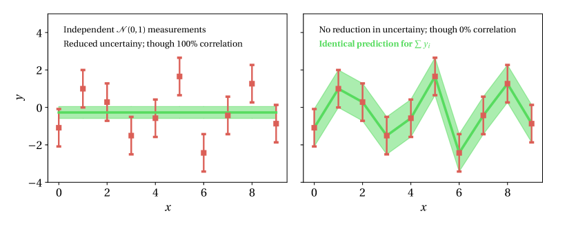
Figure 5: A horizontal line fitted to noisy data (left) and a naive model that passes through every data point (right). Despite making quite different predictions for $y$, they make identical predictions for $\sum y_{i}$.

Let us create an example closer to our TGP model and demonstrate an identical effect. In a GP with fixed hyperparameters for measurements with uniform noise $\sigma$, the covariance between prediction points $X^{\star}$ can be expressed as

$$\textsf{Cov}\mathopen{}\mathclose{{}\left[\vphantom{R_{i},R_{j}}y(X^{\star}),y(X^{\star})}\right]=K(X^{\star},X^{\star})-K(X^{\star},X)^{T}\left[K(X,X)+\sigma^{2}\right]^{-1}K(X^{\star},X)$$ (34)

where $X$ are the training points, $K$ is the choice of kernel function, and $\sigma^{2}$ is the noise. This expression is somewhat intractable due to the inverse matrix. Thus we consider $X=X^{\star}$ and a simplified covariance,

$$K_{ij}=a+b\delta_{ij}.$$ (35)

With this choice, one can compute $\textsf{Cov}\mathopen{}\mathclose{{}\left[\vphantom{R_{i},R_{j}}y(X^{\star}),y(X^{\star})}\right]$ and the sum over its elements analytically. The covariance may be written as

$$\textsf{Cov}\mathopen{}\mathclose{{}\left[\vphantom{R_{i},R_{j}}y(X^{\star}),y(X^{\star})}\right]=A\begin{pmatrix}D&a\sigma^{2}&\cdots&a\sigma^{2}\\ a\sigma^{2}&D&\cdots&a\sigma^{2}\\ \vdots&\vdots&\ddots&\vdots\\ a\sigma^{2}&a\sigma^{2}&\cdots&D\\ \end{pmatrix}$$ (36)

where

$$A \equiv\frac{\sigma^{2}}{(b+\sigma^{2})(na+b+\sigma^{2})}$$ (37)

$$D \equiv b(na+b)+(a+b)\sigma^{2}.$$ (38)

Summing the elements results in,

$$\sum\textsf{Cov}\mathopen{}\mathclose{{}\left[\vphantom{R_{i},R_{j}}y(X^{\star}),y(X^{\star})}\right]=\frac{n(na+b)\sigma^{2}}{na+b+\sigma^{2}}$$ (39)

where $n$ represents the size of $X^{\star}$. By performing a Taylor expansion about $\sigma=0$, we discover

$$\sum\textsf{Cov}\mathopen{}\mathclose{{}\left[\vphantom{R_{i},R_{j}}y(X^{\star}),y(X^{\star})}\right]=n\sigma^{2}+\mathcal{O}(\sigma^{4}).$$ (40)

Although the structure eq. 35 isn’t particularly realistic, our result holds for any $a$, including $0\%$ and $100\%$ correlation. When $C_{i}\approx C\equiv\text{const.}$, the uncertainties from the TGP and naive method are both around $C\sqrt{n}\sigma$. The decrease in variance and increase in covariance cancel in the TGP uncertainties. For the case in which the prediction locations are denser than the input locations, this result may hold if the TGP predictions don’t change substantially between input locations.

References

- [1] The Muon Collaboration, Final Report of the Muon E821 Anomalous Magnetic Moment Measurement at BNL, Phys. Rev. D 73 (2006) 072003 [hep-ex/0602035].
- [2] The Muon Collaboration, Measurement of the Positive Muon Anomalous Magnetic Moment to 0.46 ppm, Phys. Rev. Lett. 126 (2021) 141801 [2104.03281].
- [3] P. Athron, C. Balázs, D.H.J. Jacob, W. Kotlarski, D. Stöckinger and H. Stöckinger-Kim, New physics explanations of in light of the FNAL muon measurement, JHEP 09 (2021) 080 [2104.03691].
- [4] T. Aoyama et al., The anomalous magnetic moment of the muon in the Standard Model, Phys. Rept. 887 (2020) 1 [2006.04822].
- [5] P. Athron, A. Fowlie, C.-T. Lu, L. Wu, Y. Wu and B. Zhu, Hadronic uncertainties versus new physics for the W boson mass and Muon anomalies, Nature Commun. 14 (2023) 659 [2204.03996].
- [6] T. Teubner, K. Hagiwara, R. Liao, A.D. Martin and D. Nomura, Update of of the Muon and Delta Alpha, Chin. Phys. C 34 (2010) 728 [1001.5401].
- [7] The KLOE-2 Collaboration, Combination of KLOE measurements and determination of in the energy range , JHEP 03 (2018) 173 [1711.03085].
- [8] The BaBar Collaboration, Study of the process using initial state radiation, Phys. Rev. D 97 (2018) 052007 [1801.02960].
- [9] The BaBar Collaboration, The , , and Cross Sections Measured with Initial-State Radiation, Phys. Rev. D 76 (2007) 092005 [0708.2461], [Erratum: Phys. Rev. D 77 (2008) 119902].
- [10] The BaBar Collaboration, Measurement of the cross section using initial-state radiation at BaBar, Phys. Rev. D 96 (2017) 092009 [1709.01171].
- [11] The BaBar Collaboration, Study of the reactions and at center-of-mass energies from threshold to 4.35 GeV using initial-state radiation, Phys. Rev. D 98 (2018) 112015 [1810.11962].
- [12] The SND Collaboration, Study of the reaction with the SND detector at the VEPP-2M collider, Phys. Rev. D 93 (2016) 092001 [1601.08061].
- [13] The CMD-3 Collaboration, Study of the process in the c.m. energy range 1394 – 2005 MeV with the CMD-3 detector, Phys. Lett. B 773 (2017) 150 [1706.06267].
- [14] The CMD-3 Collaboration, Study of the process in the C.M. Energy range 1.6 – 2.0 GeV with the CMD-3 detector, Phys. Lett. B 792 (2019) 419 [1902.06449].
- [15] B.E. Lautrup and E. De Rafael, Calculation of the sixth-order contribution from the fourth-order vacuum polarization to the difference of the anomalous magnetic moments of muon and electron, Phys. Rev. 174 (1968) 1835.
- [16] S.J. Brodsky and E. De Rafael, Suggested Boson-Lepton Pair Couplings And The Anomalous Magnetic Moment Of The Muon, Phys. Rev. 168 (1968) 1620.
- [17] H. Wittig, Progress on from Lattice QCD, in Proceedings of the 2023 Electroweak Session of the 57th Rencontres de Moriond, June, 2023 [2306.04165].
- [18] G. Benton, D. Boito, M. Golterman, A. Keshavarzi, K. Maltman and S. Peris, Data-driven determination of the light-quark connected component of the intermediate-window contribution to the muon , 2306.16808.
- [19] S. Borsanyi et al., Leading hadronic contribution to the muon magnetic moment from lattice QCD, Nature 593 (2021) 51 [2002.12347].
- [20] M. Cè et al., Window observable for the hadronic vacuum polarization contribution to the muon from lattice QCD, Phys. Rev. D 106 (2022) 114502 [2206.06582].
- [21] The Extended Twisted Mass Collaboration, Lattice calculation of the short and intermediate time-distance hadronic vacuum polarization contributions to the muon magnetic moment using twisted-mass fermions, Phys. Rev. D 107 (2023) 074506 [2206.15084].
- [22] T. Blum et al., An update of Euclidean windows of the hadronic vacuum polarization, 2301.08696.
- [23] P. Masjuan, A. Miranda and P. Roig, data-driven evaluation of Euclidean windows for the hadronic vacuum polarization, 2305.20005.
- [24] The CMD-3 Collaboration, Measurement of the cross section from threshold to 1.2 GeV with the CMD-3 detector, 2302.08834.
- [25] The CMD-2 Collaboration, High-statistics measurement of the pion form factor in the rho-meson energy range with the CMD-2 detector, Phys. Lett. B 648 (2007) 28 [hep-ex/0610021].
- [26] M. Hansen, A. Lupo and N. Tantalo, Extraction of spectral densities from lattice correlators, Phys. Rev. D 99 (2019) 094508 [1903.06476].
- [27] The Extended Twisted Mass Collaboration (ETMC) Collaboration, Probing the Energy-Smeared Ratio Using Lattice QCD, Phys. Rev. Lett. 130 (2023) 241901 [2212.08467].
- [28] A. Fowlie, “kingpin — treed Gaussian process algorithm.” https://github.com/andrewfowlie/kingpin, 2023.
- [29] M. Davier, A. Hoecker, B. Malaescu, C.Z. Yuan and Z. Zhang, Reevaluation of the hadronic contribution to the muon magnetic anomaly using new cross section data from BaBar, Eur. Phys. J. C 66 (2010) 1 [0908.4300].
- [30] M. Davier, A. Hoecker, B. Malaescu and Z. Zhang, Reevaluation of the hadronic vacuum polarisation contributions to the Standard Model predictions of the muon and using newest hadronic cross-section data, Eur. Phys. J. C 77 (2017) 827 [1706.09436].
- [31] M. Davier, A. Hoecker, B. Malaescu and Z. Zhang, A new evaluation of the hadronic vacuum polarisation contributions to the muon anomalous magnetic moment and to , Eur. Phys. J. C 80 (2020) 241 [1908.00921], [Erratum: Eur. Phys. J. C 80 (2020) 410].
- [32] The Particle Data Group, Review of Particle Physics, PTEP 2022 (2022) 083C01.
- [33] A. Keshavarzi, D. Nomura and T. Teubner, Muon and : a new data-based analysis, Phys. Rev. D 97 (2018) 114025 [1802.02995].
- [34] A. Keshavarzi, D. Nomura and T. Teubner, of charged leptons, , and the hyperfine splitting of muonium, Phys. Rev. D 101 (2020) 014029 [1911.00367].
- [35] C.K. Williams and C.E. Rasmussen, Gaussian processes for machine learning, MIT press, Cambridge, MA (2006).
- [36] D.J. MacKay, Information theory, inference and learning algorithms, Cambridge University Press (2003).
- [37] D. Foreman-Mackey, E. Agol, S. Ambikasaran and R. Angus, Fast and Scalable Gaussian Process Modeling with Applications to Astronomical Time Series, The Astronomical Journal 154 (2017) 220 [1703.09710].
- [38] S.O. Rice, Mathematical analysis of random noise, The Bell System Technical Journal 23 (1944) 282.
- [39] R.B. Gramacy and H.K.H. Lee, Bayesian treed Gaussian process models with an application to computer modeling, J. Amer. Statist. Assoc. 103 (2008) 1119 [0710.4536].
- [40] R.B. Gramacy, Surrogates: Gaussian Process Modeling, Design and Optimization for the Applied Sciences, Chapman Hall/CRC, Boca Raton, Florida (2020).
- [41] H.A. Chipman, E.I. George and R.E. McCulloch, Bayesian CART model search, J. Amer. Statist. Assoc. 93 (1998) 935.
- [42] H.A. Chipman, E.I. George and R.E. McCulloch, Bayesian treed models, Machine Learning 48 (2002) 299.
- [43] D. Denison, N. Adams, C. Holmes and D. Hand, Bayesian partition modelling, Computational Statistics & Data Analysis 38 (2002) 475.
- [44] H.-M. Kim, B.K. Mallick and C.C. Holmes, Analyzing nonstationary spatial data using piecewise Gaussian processes, J. Amer. Statist. Assoc. 100 (2005) 653.
- [45] A. Lederer, A.J.O. Conejo, K. Maier, W. Xiao, J. Umlauft and S. Hirche, Real-time regression with dividing local Gaussian processes, 2006.09446.
- [46] C.J. Paciorek and M.J. Schervish, Nonstationary Covariance Functions for Gaussian Process Regression, in Proceedings of the 16th International Conference on Neural Information Processing Systems, NIPS’03, (Cambridge, MA, USA), p. 273–280, MIT Press, 2003.
- [47] A. Damianou and N.D. Lawrence, Deep Gaussian Processes, in Proceedings of the Sixteenth International Conference on Artificial Intelligence and Statistics, C.M. Carvalho and P. Ravikumar, eds., vol. 31 of Proceedings of Machine Learning Research, (Scottsdale, Arizona, USA), pp. 207–215, PMLR, May, 2013.
- [48] A.G. Wilson, Z. Hu, R. Salakhutdinov and E.P. Xing, Deep Kernel Learning, in Proceedings of the 19th International Conference on Artificial Intelligence and Statistics, A. Gretton and C.C. Robert, eds., vol. 51 of Proceedings of Machine Learning Research, (Cadiz, Spain), pp. 370–378, PMLR, 09–11 May, 2016 [1511.02222].
- [49] V. Tolvanen, P. Jylänki and A. Vehtari, Expectation propagation for nonstationary heteroscedastic Gaussian process regression, in 2014 IEEE International Workshop on Machine Learning for Signal Processing (MLSP), pp. 1–6, 2014, DOI.
- [50] M. Heinonen, H. Mannerström, J. Rousu, S. Kaski and H. Lähdesmäki, Non-Stationary Gaussian Process Regression with Hamiltonian Monte Carlo, in Proceedings of the 19th International Conference on Artificial Intelligence and Statistics, A. Gretton and C.C. Robert, eds., vol. 51 of Proceedings of Machine Learning Research, (Cadiz, Spain), pp. 732–740, PMLR, 09–11 May, 2016.
- [51] A. Sauer, R.B. Gramacy and D. Higdon, Active learning for deep Gaussian process surrogates, Technometrics (2022) 1 [2012.08015].
- [52] A. Sauer, A. Cooper and R.B. Gramacy, Vecchia-approximated Deep Gaussian Processes for Computer Experiments, Journal of Computational and Graphical Statistics (2022) 1 [2204.02904].
- [53] P.J. Green, Reversible jump Markov chain Monte Carlo computation and Bayesian model determination, Biometrika 82 (1995) 711.
- [54] P.J. Green and D.I. Hastie, Reversible jump MCMC, Genetics 155 (2009) 1391.
- [55] D.I. Hastie and P.J. Green, Model choice using reversible jump Markov chain Monte Carlo, Statistica Neerlandica 66 (2012) 309.
- [56] S.A. Sisson, Transdimensional Markov chains: A decade of progress and future perspectives, J. Amer. Statist. Assoc. 100 (2005) 1077.
- [57] A. O’Hagan, Bayes–Hermite quadrature, Journal of Statistical Planning and Inference 29 (1991) 245.
- [58] Z. Ghahramani and C. Rasmussen, Bayesian Monte Carlo, in Advances in Neural Information Processing Systems, S. Becker, S. Thrun and K. Obermayer, eds., vol. 15, MIT Press, 2002.
- [59] M. Fisher, C. Oates, C. Powell and A. Teckentrup, A Locally Adaptive Bayesian Cubature Method, in Proceedings of the Twenty Third International Conference on Artificial Intelligence and Statistics, S. Chiappa and R. Calandra, eds., vol. 108 of Proceedings of Machine Learning Research, pp. 1265–1275, PMLR, 26–28 Aug, 2020 [1910.02995].
- [60] R. Jagadeeswaran and F.J. Hickernell, Fast automatic Bayesian cubature using lattice sampling, Statistics and Computing 29 (2019) 1215 [1809.09803].
- [61] F.-X. Briol, C.J. Oates, M. Girolami, M.A. Osborne and D. Sejdinovic, Probabilistic Integration: A Role in Statistical Computation?, Statistical Science 34 (2019) 1 [1512.00933].
- [62] H. Zhu, X. Liu, R. Kang, Z. Shen, S. Flaxman and F.-X. Briol, Bayesian Probabilistic Numerical Integration with Tree-Based Models, in Advances in Neural Information Processing Systems, H. Larochelle, M. Ranzato, R. Hadsell, M. Balcan and H. Lin, eds., vol. 33, pp. 5837–5849, Curran Associates, Inc., 2020.
- [63] D.J. MacKay, Information-based objective functions for active data selection, Neural computation 4 (1992) 590.
- [64] S. Seo, M. Wallat, T. Graepel and K. Obermayer, Gaussian process regression: Active data selection and test point rejection, in Proceedings of the IEEE-INNS-ENNS International Joint Conference on Neural Networks. IJCNN 2000. Neural Computing: New Challenges and Perspectives for the New Millennium, vol. 3, pp. 241–246, 2000, DOI.
- [65] P. Wei, X. Zhang and M. Beer, Adaptive experiment design for probabilistic integration, Computer Methods in Applied Mechanics and Engineering 365 (2020) 113035.
- [66] R.B. Gramacy and H.K.H. Lee, Adaptive Design and Analysis of Supercomputer Experiments, Technometrics 51 (2009) 130 [0805.4359].
- [67] The Particle Data Group, “Data files and plots of cross-sections and related quantities in the 2022 Review of Particle Physics.” https://pdg.lbl.gov/2023/hadronic-xsections/hadron.html, 2023.
- [68] V.V. Ezhela, S.B. Lugovsky and O.V. Zenin, Hadronic part of the muon estimated on the evaluated data compilation, hep-ph/0312114.
- [69] R. Kumar, C. Carroll, A. Hartikainen and O. Martin, ArviZ a unified library for exploratory analysis of Bayesian models in Python, Journal of Open Source Software 4 (2019) 1143.
- [70] A. Vehtari, A. Gelman, D. Simpson, B. Carpenter and P.-C. Bürkner, Rank-normalization, folding, and localization: An improved for assessing convergence of MCMC, Bayesian Analysis 16 (2019) [1903.08008].
- [71] Q. Li, “Code and data associated with this paper.” https://github.com/qiao688/TGP, 2023.
- [72] W.H. Press, S.A. Teukolsky, W.T. Vetterling and B.P. Flannery, Numerical recipes in C: The art of scientific computing, Cambridge University Press (1992).
- [73] M.W. Seeger, C.K.I. Williams and N.D. Lawrence, Fast Forward Selection to Speed Up Sparse Gaussian Process Regression, in Proceedings of the Ninth International Workshop on Artificial Intelligence and Statistics, C.M. Bishop and B.J. Frey, eds., vol. R4 of Proceedings of Machine Learning Research, pp. 254–261, PMLR, 03–06 Jan, 2003.
- [74] J. Quinonero-Candela and C.E. Rasmussen, A unifying view of sparse approximate Gaussian process regression, The Journal of Machine Learning Research 6 (2005) 1939.
- [75] E. Snelson and Z. Ghahramani, Local and global sparse Gaussian process approximations, in Proceedings of the Eleventh International Conference on Artificial Intelligence and Statistics, M. Meila and X. Shen, eds., vol. 2 of Proceedings of Machine Learning Research, (San Juan, Puerto Rico), pp. 524–531, PMLR, 21–24 Mar, 2007.
- [76] H. Liu, Y.-S. Ong, X. Shen and J. Cai, When Gaussian Process Meets Big Data: A Review of Scalable GPs, IEEE Transactions on Neural Networks and Learning Systems 31 (2020) 4405.
- [77] J. Hensman, N. Fusi and N.D. Lawrence, Gaussian Processes for Big Data, in Proceedings of the Twenty-Ninth Conference on Uncertainty in Artificial Intelligence, pp. 282–290, 2013 [1309.6835].
- [78] J.-B. Delisle, N. Hara and D. Ségransan, Efficient modeling of correlated noise, Astronomy & Astrophysics 638 (2020) A95 [2004.106].