Capturing functional connectomics using Riemannian partial least squares

Abstract

For neurological disorders and diseases, functional and anatomical connectomes of the human brain can be used to better inform targeted interventions and treatment strategies. Functional magnetic resonance imaging (fMRI) is a non-invasive neuroimaging technique that captures spatio-temporal brain function through blood flow over time. FMRI can be used to study the functional connectome through the functional connectivity matrix; that is, Pearson’s correlation matrix between time series from the regions of interest of an fMRI image. One approach to analysing functional connectivity is using partial least squares (PLS), a multivariate regression technique designed for high-dimensional predictor data. However, analysing functional connectivity with PLS ignores a key property of the functional connectivity matrix; namely, these matrices are positive definite. To account for this, we introduce a generalisation of PLS to Riemannian manifolds, called R-PLS, and apply it to symmetric positive definite matrices with the affine invariant geometry. We apply R-PLS to two functional imaging datasets: COBRE, which investigates functional differences between schizophrenic patients and healthy controls, and; ABIDE, which compares people with autism spectrum disorder and neurotypical controls. Using the variable importance in the projection statistic on the results of R-PLS, we identify key functional connections in each dataset that are well represented in the literature. Given the generality of R-PLS, this method has potential to open up new avenues for multi-model imaging analysis linking structural and functional connectomics.

[acronym]long-short

Introduction

The functional and anatomical connections of the human brain form complex networks that link the infrastructure of our minds. Understanding these connectomes has the potential to provide insight into the effect of neurological diseases which can be used to better inform targeted interventions and treatment strategies[(1), (2)]. In particular, the functional connectome can shed new light onto neurological conditions such as schizophrenia and autism spectrum disorder (ASD), two conditions that alter brain function from healthy, neurotypical controls[(3), (4)].

A popular approach used to investigate brain function is functional magnetic resonance imaging (fMRI), a non-invasive neuroimaging technique that measures blood flow through the brain over time[(5)]. An fMRI image is a complex spatio-temporal picture of the brain with voxels (volumetric pixels) describing the spatial location and a time series for each voxel describing the blood flow over time. To reduce the spatial complexity, voxels can be collated into user-specified regions of interest (ROIs). Functional connectomes can then be investigated through the Pearson correlation matrix between ROIs, known as the functional connectivity matrix.

One approach to investigating functional connectivity is using the partial least squares (PLS) regression method. Introduced by Wold (1975)[(6)] for use in chemometrics, PLS is an extension of multivariate multiple regression to high-dimensional data that predicts the response data from a set of lower-dimensional latent variables constructed from the predictor data. Popularised for fMRI by McIntosh et. al. (1996)[(7)], PLS has been used to explore the relationships between fMRI data and either behavioural data, experimental designs, or seed region activation (Krishnan2011, ). However, standard PLS ignores the structure of functional connectivity data – functional connectivity matrices are correlation matrices and hence positive definite.

The space of $R\times R$ symmetric positive definite matrices – which includes functional connectivity matrices – forms a convex cone in $R(R+1)/2$-dimensional Euclidean space. However, when considered with the affine invariant geometryPennec2006 , the space of symmetric positive definite matrices becomes a complete Riemannian manifold with non-positive curvature. By considering this non-linear geometry on symmetric positive definite matrices we can glean interesting new insights into functional connectivity (see Pennec et. al. (2019)Pennec2019 and citations therein).

Here we propose an extension of the PLS model to allow Riemannian manifold response and predictor data, which we call Riemannian partial least squares (R-PLS). The R-PLS model then allows us to predict from functional connectivity data while accounting for the intricate relationships enforced by the positive definite criteria. To fit the R-PLS model, we propose the tangent non-linear iterative partial least squares (tNIPALS) algorithm, which is related to previously proposed applications of PLS for functional connectivity data in the literatureWong2018 ; Chu2020 ; Zhang2018a ; Perez2013 . We determine the optimal number of latent variables using cross validation. To aid in interpretability of the high-dimensional functional connectivity data, we determine significant functional connections identified by R-PLS using permutation tests on the variable importance in the projection (VIP) statisticWold1993 , a popular measure of variable importance from standard PLS.

We apply R-PLS to two datasets and two different ROI atlases to demonstrate its versatility. First is the COBRE datasetAine2017 which investigates differences in functional connectivity between health controls and patients with schizophrenia; we consider the fMRI in the COBRE dataset in the functional multi-subject dictionary learning (MSDL) atlasVaroquaux2010 . Second is the ABIDE datasetCraddock2013 which investigates differences in functional connectivity between typical health controls and subjects with ASD; we consider the ABIDE data in the automated anatomic labelling (AAL) atlas Tzourio-Mazoyer2002 .

Results

COBRE

Ten-fold cross validation showed that $K=2$ latent variables was the most parsimonious, within one standard error of the minimum root mean square error (RMSE) ($K=3$). When compared with Euclidean PLS using raw and Fisher-transformed correlations, R-PLS outperformed both methods across all metrics except for specificity in group prediction (Table 1) . However, all three methods produced similar results for every metric.

A permutation test of the $\mathrm{VIP}$ statistic (Equation 5) with $200$ permutations found $45$ significant functional connections between ROIs as being predictive of age and subject group (Figure 1). To aid interpretability, we have reduced the $39$ ROIs of the MSDL atlas into the $17$ resting state networks associated to the atlas Varoquaux2011 by taking the mean coefficient value within the ROIs of each network, as suggested by Wong et. al. (2018) Wong2018 .

An increase in subject age tended towards a decrease of within-network connectivity (as measured by a mean decrease in functional connectivity within-networks) with particular emphasis on the auditory network, cingulate insula, and left and right ventral attention networks (Figure 1 (left)). Further, increased age was associated with an increase in between-network connectivity with focus on connectivity involving the cingulate insula and the motor network.

For subjects in the schizophrenic group, the basal ganglia exhibited both increased and decreased connectivity with other networks (Figure 1 (right)). In particular, there was a decrease in connectivity between the basal ganglia and the cerebellum and salience networks, whereas we observed an increase in connectivity between the basal ganglia and auditory and language networks for the schizophrenic group. We also note that the default mode network was highly discriminatory for the schizophrenic group showing increased within-network connectivity and both increased and decreased between-network connectivity.

ABIDE

Ten-fold cross validation found $K=3$ latent variables was the most parsimonious, within one standard error of the minimum RMSE ($K=6$). When compared with Euclidean PLS using the raw and Fisher-transformed correlations, R-PLS outperformed both methods across all metrics except for specificity in group classification (Table 1). In particular, the $R^{2}$ value for R-PLS was substantially larger than the Euclidean methods.

A permutation test of the $\mathrm{VIP}$ statistic (Equation 5) with $200$ permutations found $208$ significant functional connections between ROIs as being predictive of age, subject group, sex and eye status (Figure 2). We aid interpretability by associating the $116$ ROIs of the AAL atlas to the seven resting-state networks suggested by Parente and Colosimo (2020)Parente2020 and an eighth containing the cerebellum and vermis, which we call the cerebellum network.

In the ABIDE dataset, increased age was associated to both increased and decreased functional connectivity within resting-state networks (Figure 2 (a)). Although we observed increased between-network connectivity for the thalamus and occipital networks, the cerebellum and default mode network exhibited decreased between-network connectivity with age.

For subjects with ASD we observed increased within-network connectivity with the exception of the limbic network and the thalamus (Figure 2 (b)). We also observed decreased between-network connectivity particularly for the cerebellum and the limbic networks. We observed the same connectivity patterns for subject sex (Figure 2 (c))

For subjects with their eyes closed, our model suggests there was decreased within-network connectivity (Figure 2 (d)). With the exception of the default mode network and the limbic network, we saw decreased between-network connectivity with particular emphasis on the occipital network.

Discussion

The R-PLS model has identified many functional connections associated to age, ASD, schizophrenia, sex, and eye status that are well represented in the literature. In both the COBRE and ABIDE datasets, we identified the reduction of within-network connectivity with age that has been previously observed(Varangis2019, ; Edde2021, ; Ferreira2016, ), with exceptions in the temporo-parietal, fronto-parietal, limbic and thalamus networks in the ABIDE dataset and the salience network in the COBRE dataset, which all show an increase in connectivity with age. Further, both datasets exhibit the decreased connectivity with the default mode network, consistent with existing literature (Tomasi2011, ; Pinero2014, ).

For subjects with ASD, the decreased connectivity with the cerebellumRamos2019 and the limbicPascual2018 networks have been previously observed. However, the decreased between-network connectivity suggested by R-PLS is in contradiction with existing literature(Assaf2010, ; Wong2018, ); in particular, Wong et. al. (2018)Wong2018 showed an increase in between-network connectivity associated to ASD on the full ABIDE dataset using logistic regression. Also, observe that the connectivity for subject sex is highly correlated with the connectivity for the ASD group. Although interactions between subject sex and ASD have been identified (Smith2019, ), we believe this highlights a possible limitation of R-PLS and requires further investigation in future research.

The role of the basal ganglia in schizophrenic patients has been previously observed, particularly the decrease in connectivity between the salience network and the basal ganglia (Zhang2019, ; Orliac2013, ) and the decreased connectivity between the cerebellum and basal ganglia (Duan2015, ). Further, the connectivity patterns involving the default mode network have been previously reported in schizophrenic patients (Karbasforoushan2012, ; Woodward2011, ; Dong2018, ; Yu2012, ; Wang2015, ).

The results for eye status during scan are also well represented in the literature. The decreased within-network connectivity for the default mode network for patients with closed eyes has been previously reported by Yan et. al. (2009)Yan2009 , and the increased between-network connectivity for the default mode network has recently been discussed by Han et. al. (2023)Han2023 . Further, the observed decrease in connectivity for the occipital network agrees with Agcaoglu et. al. (2019)Agcaoglu2019 .

The use of the VIP statistic to identify significant connections in functional connectivity has not been previously studied. We have demonstrated that this statistic can identify many functional connections that have been addressed previously in the literature, but it is not without its limitations. First, with our focus on generalising partial least squares to Riemannian manifolds, the VIP statistic does not take into account the Riemannian geometry we are considering. This is mitigated by the tangent space approximation we are performing, which directly accounts for the geometry of the data, but further research could help better generalise the VIP statistic for R-PLS. Further, the VIP statistic associates the effects of a single predictor on the full multivariate response. In situations like we consider here, this makes it difficult to determine which functional connections are associated to which outcome variable. For example, the connectivity within the default mode network is deemed significant by the VIP statistic in the ABIDE dataset, but it is unclear whether this connectivity is significance for every outcome variable or a subset of them. Work has been done to generalise the VIP statistic when the outcome variable is multivariateRyan2023 , but further research is needed to investigate this generalisation.

These results suggest that R-PLS can provide insight into the functional connectome and how it relates to subject phenotype data. Further, due to the specification and generality of the R-PLS model, this method is readily applicable to other imaging modalities, and in particular to multimodal imaging studies. The application of R-PLS to multimodal imaging studies is an area of future research that may help to us to understand the functional networks that make up the human connectome.

Methods

Data

The International Neuroimaging Data-Sharing Initiative (INDI) is an initiative set to encourage free open access to neuroimaging datasets from around the world. We consider two datasets that are accessible as a part of the INDI.

COBRE

The Center for Biomedical Research Excellence (COBRE) have contributed structural and functional MRI images to the INDI that compare schizophrenic patients with healthy controls Aine2017 . The data were collected with single-shot full k-space echo-planar imaging with a TR of $2000$ milliseconds, matrix size of $64\times 64$ and $32$ slices (giving a voxel size of $3\times 3\times 4\,mm^{3}$). These data were downloaded using the Python package nilearn v 0.6.2, and contains $146$ subjects (Control $=74$), each with phenotype information on subject group and age; further information is available in Table S1 of the supplementary material.

The fMRI data were preprocessed using NIAK 0.17 under CentOS version 6.3 with Octave version 4.0.2 and the Minc toolkit version 0.3.18 Bellec2011 . The data were subjected to nuisance regression where we removed six motion parameters, the frame-wise displacement, five slow-drift parameters, average parameters for white matter, lateral ventricles, and global signal, as well as 5 estimates for component based noise correction Behzadi2007 .

For the COBRE dataset, we consider each fMRI in the MSDL atlas, a functional ROI decomposition of $39$ nodes across $17$ resting state networks Varoquaux2011 . Time series were extracted for each ROI by taking the mean time series across the voxels in each region.

ABIDE

The Autism Brain Imaging Data Exchange (ABIDE) is part of the Preprocessed Connectomes Project in INDI Craddock2013 . The ABIDE data is a collection of preprocessed fMRI images from $16$ international imaging sites with 539 individuals diagnosed with ASD and 573 neurotypical controls (NTC). The ABIDE initiative provides data preprocessed under four separate standard pipelines, as well as options for band-pass filtering and global signal regression.

Here we consider the $172$ subjects (NTC = $98$) of the New York University imaging site. We restrict to this site to reduce inter-site variation in imaging and because it is the largest individual imaging site. The data were collected with a 3 Tesla Allegra MRI using echo-planar imaging with a TR of $2000$ milliseconds, matrix size of $64\times 64$ and $33$ slices (giving a voxel size of $3\times 3\times 4mm^{3}$). The fMRI data were downloaded using the Python package nilearn v 0.6.2 preprocessed using the NIAK 0.7.1 pipeline Bellec2011 . The data were subjected to: motion realignment; non-uniformity correction using the median volume; motion scrubbing; nuisance regression which removed the first principal component of 6 motion parameters, their squares, mean white matter and cerebrospinal fluid signals, and low frequency drifts measured by a discrete cosine basis with a 0.01 Hz high-pass cut-off; band-pass filtering and; global signal regression. We consider the subjects preprocessed fMRI as well as subject group, age, sex, and eye status during scan (open or closed); further information is available in Table S2 of the supplementary material.

For the ABIDE dataset, we consider each fMRI in the AAL atlasTzourio-Mazoyer2002 , an anatomical atlas of $116$ nodes across the brain. Time series were extracted by taking the mean time series across the voxels in each ROI.

Partial least squares in Euclidean space

PLS is a predictive modelling technique that predicts a response matrix $\boldsymbol{Y}_{n\times q}$ from a set of predictors $\boldsymbol{X}_{n\times p}$. Originally introduced in the chemometrics literature by Wold (1975) Wold1975 , PLS has found application in bioinformatics (Nguyen2002, ), social sciences (Hulland1999, ), and neuroimaging (Krishnan2011, ; McIntosh2004, ; Lin2003, ); see Rosipal and Krämer (2006)Rosipal2006 and citations therein for further examples. As an extension of multivariate multiple regression, PLS has been shown to have better predictive accuracy than multivariate multiple regression when the standard regression assumptions are met (Garthwaite1994, ). A further advantage of PLS is that it is effective when $q>n$ or $p>n$ since it performs prediction from lower dimensional latent variables, that is, PLS constructs a new set of predictor variables from $\boldsymbol{X}$ to predict $\boldsymbol{Y}$ (Garthwaite1994, ).

Let $\boldsymbol{X}_{n\times p}$ and $\boldsymbol{Y}_{n\times q}$ be predictor and response matrices respectively. Suppose $\boldsymbol{X}$ and $\boldsymbol{Y}$ are column centred, that is, suppose the means of each column of $\boldsymbol{X}$ and $\boldsymbol{Y}$ are $0$. PLS proposes the existence of $L\leq\min\{p,n\}$ latent variables such that $\boldsymbol{X}$ and $\boldsymbol{Y}$ decompose into a set of scores matrices $\boldsymbol{T}_{n\times L}$ and $\boldsymbol{U}_{n\times L}$, and loadings matrices $\boldsymbol{P}_{p\times L}$ and $\boldsymbol{Q}_{q\times L}$ with

$$\boldsymbol{X} =\boldsymbol{T}\boldsymbol{P}^{T}+\boldsymbol{E}\,,$$ (1)

$$\boldsymbol{Y} =\boldsymbol{U}\boldsymbol{Q}^{T}+\boldsymbol{F}\,,$$ (2)

where $\boldsymbol{E}_{n\times p}$ and $\boldsymbol{F}_{n\times q}$ are error matrices, assumed to be a small as possible (Geladi1986, ), and the superscript $T$ denotes the matrix transpose. Further, PLS assumes that there is a diagonal matrix $\boldsymbol{B}_{L\times L}$ with

$$\boldsymbol{U}=\boldsymbol{T}\boldsymbol{B}+\boldsymbol{H}_{n\times L}\,,$$ (3)

where $\boldsymbol{H}$ is a matrix of residuals. Equations 1 and 2 are called the outer relationships while Equation 3 defines the inner relationship that connects $\boldsymbol{X}$ and $\boldsymbol{Y}$. Combining the inner relationship and the outer relationship for $\boldsymbol{Y}$ gives

$$\boldsymbol{Y}=\boldsymbol{T}\boldsymbol{B}\boldsymbol{Q}^{T}+(\boldsymbol{H}\boldsymbol{Q}^{T}+\boldsymbol{F})\,,$$

which highlights that $\boldsymbol{Y}$ is a regression on the latent scores $\boldsymbol{T}$. Further, notice that the error in $\boldsymbol{Y}$ is given by $\boldsymbol{H}\boldsymbol{Q}^{T}+\boldsymbol{F}$, that is, error in $\boldsymbol{Y}$ is a combination of error inherent to the response data ($\boldsymbol{F}$) and error from the estimation of the inner relationship ($\boldsymbol{H}\boldsymbol{Q}^{T}$). The inclusion of the residual matrix $\boldsymbol{H}$ can complicate discussion of the PLS method, so it is common to consider the estimated inner relationship $\boldsymbol{\hat{U}}\approx\boldsymbol{T}\boldsymbol{B}$ instead (Hoskuldsson1988, ; Geladi1986, ).

Estimation of the PLS model (Equations 1–3) is commonly done through the non-linear iterative partial least squares (NIPALS) algorithm (Algorithm S1 in the supplementary material). The inputs for the NIPALS algorithm are the data matrices $\boldsymbol{X}$ and $\boldsymbol{Y}$ and the pre-specified number of latent variables $K$; noting that the true number of latent variables $L$ is unknown, the value $K$ can be chosen with methods such as cross validation. The NIPALS algorithm outputs estimates of the scores, loadings, and regression coefficients as well as matrices $\boldsymbol{W}_{p\times K}$ and $\boldsymbol{C}_{q\times K}$ known as the weights. The weight matrices $\boldsymbol{W}$ and $\boldsymbol{C}$ are linear transformations of $\boldsymbol{P}$ and $\boldsymbol{Q}$ that more efficiently fit the PLS model and are defined within the NIPALS algorithm; see the supplementary material for further information. Using the results of the NIPALS algorithm and Equations 1–3, we can write

$$\boldsymbol{\hat{Y}}=\boldsymbol{X}\boldsymbol{\hat{\beta}}_{PLS}$$

where

$$\boldsymbol{\hat{\beta}}_{PLS}=\boldsymbol{W}(\boldsymbol{P}^{T}\boldsymbol{W})^{-1}\boldsymbol{B}\boldsymbol{C}^{T}$$ (4)

is the matrix of regression coefficients. Using $\boldsymbol{\hat{\beta}}_{PLS}$ we see that PLS is a linear regression technique similar to ordinary least squares and ridge regression.

The VIP statistic

To determine significant predictors of the response variables in the PLS model, we use the VIP statistic (Wold1993, ). Suppose there are $p$ predictor variables, $q$ response variables, and $K$ latent variables extracted using NIPALS. Following Tennenhaus (1998)Tenenhaus1998 , the VIP statistic for the $j^{th}$ predictor variable is

$$\mathrm{VIP}_{j}=\sqrt{\frac{p}{\mathrm{Rd}(\boldsymbol{Y},\boldsymbol{T})}\sum\limits_{k=1}^{K}\mathrm{Rd}(\boldsymbol{Y},\boldsymbol{t_{k}})\left(w_{jk}\right)^{2}}\,,$$ (5)

where $\boldsymbol{t}_{k}$ is the $k^{th}$ column of the score matrix $\boldsymbol{T}$, $w_{jk}$ is the $k^{th}$ weight for the $j^{th}$ predictor, $\mathrm{Rd}(\boldsymbol{Y},\boldsymbol{t_{k}})=\frac{1}{q}\sum\limits_{i=1}^{q}\mathrm{cor}(\boldsymbol{Y}_{i},\boldsymbol{t}_{k})^{2}$, and $\mathrm{Rd}(\boldsymbol{Y},\boldsymbol{T})=\sum\limits_{k=1}^{K}\mathrm{Rd}(\boldsymbol{Y},\boldsymbol{t_{k}})$. The coefficient $\mathrm{cor}(\boldsymbol{Y}_{i},\boldsymbol{t}_{k})^{2}$ is the squared correlation between the $i^{th}$ response variable and the $k^{th}$ score. The denominator $\mathrm{Rd}(\boldsymbol{Y},\boldsymbol{T})$ in Equation 5 measures the proportion of variance in $\boldsymbol{Y}$ explained by $\boldsymbol{T}$, and the numerator $\mathrm{Rd}(\boldsymbol{Y},\boldsymbol{t_{k}})(w_{jk})^{2}$ measures the proportion of variance in $\boldsymbol{Y}$ described by the $k^{th}$ latent variable that is explained by the $j^{th}$ predictor (Tran2014, ). Thus the VIP statistic measures the influence of each predictor on the explained variation in the model (Galindo2014, ).

Commonly, the “greater than one”  rule is used to find predictors significantly associated with the response. However, this rule is motivated by the mathematical properties of $\mathrm{VIP}_{j}$ rather than statistical properties (Tran2014, ). Thus, we use a permutation test to determine significance of $\mathrm{VIP}_{j}$. This is an alternative to Afanador et. al. (2013)Afanador2013 who used $95\%$ jackknife confidence intervals to determine significance of VIP.

Specifically, for each predictor variable $j$ we permute the values $H$ times. For each permutation $h=1,2,\dots,H$ we refit the PLS model and calculate $\mathrm{VIP}_{j,h}$. The P-value for the $j^{th}$ $\mathrm{VIP}$ score is then

$$\text{{P}-value}_{j}=\frac{\#\,\left\{\mathrm{VIP}_{j,h}>\mathrm{VIP}_{j}\right\}}{H}\,.$$ (6)

For our data, the predictors are functional connectivity matrices. Thus, we know a priori that the diagonal elements are uninformative since they are identically one. Hence, if predictor $j$ describes a diagonal element we set $\text{{P}-value}_{j}=1$ for all $i$. To account for the multiple comparisons problem, we adjust all P-values using the false discovery rateBenjamini1995 and determine significance at a significance level of $\alpha=0.05$.

Mathematical preliminaries

Riemannian manifolds

Intuitively speaking, a Riemannian manifold $M$ is a space where we can perform calculus, measure distances, and measure angles between tangent vectors. More specifically, a smooth $d$-dimensional manifold $M$ is a connected, Hausdorff, second countable topological space that is covered by a set of coordinate charts $\{(U_{i},\varphi_{i}:U_{i}\rightarrow\mathbb{R}^{d})\}_{i\in I}$, defined by some indexing set $I$, such that every point in $M$ belongs to a $U_{i}$ for some $i\in I$ and the intersection maps $\varphi_{i}\circ\varphi_{j}^{-1}$ are smooth as maps $\mathbb{R}^{d}\rightarrow\mathbb{R}^{d}$ for every $i,j\in I$. These coordinate charts make the space $M$ “locally Euclidean” in the sense that every point has a neighbourhood that looks like Euclidean space. Since concepts from differential calculus are local in nature, the construction of a smooth manifold allows us to perform calculus on these more general spaces.

An important concept in the study of manifolds is the tangent bundle $TM=\bigsqcup_{a\in M}T_{a}M$, where $T_{a}M$ is the tangent space at $a$. The space $T_{a}M$ is defined as the set of equivalence classes of curves through $a$ such that $\gamma_{1}$ and $\gamma_{2}$ are equivalent if $\gamma_{1}^{\prime}(0)=\gamma_{2}^{\prime}(0)$, where the prime denotes the derivative. Then $T_{a}M$ is a vector space that generalises the notion of vectors tangent to a surface to arbitrary smooth manifolds.

A Riemannian manifold is a manifold $M$ together with a smooth map $g:M\times TM\times TM\rightarrow\mathbb{R}$ such that $g(a,\cdot,\cdot)=g_{a}:T_{a}M\times T_{a}M\rightarrow\mathbb{R}$ is an inner product for every $a\in M$. The Riemannian metric $g$ allows us to measure angles between tangent vectors and measure distances between points on the manifold $M$. Further, $g$ is used to define geodesics (locally length minimising curves) $\gamma:[t_{0},t_{1}]\rightarrow M$ between two points $a,b\in M$. We only consider complete Riemannian manifolds here, which are spaces where every geodesic $\gamma$ has domain $\mathbb{R}$.

Through geodesics we get the concepts of the Riemannian exponential and logarithm maps which allow us to smoothly move between the manifold and the tangent space. The Riemannian exponential at a point $a\in M$ is a map $\operatorname{Exp}_{a}:T_{a}M\rightarrow M$ defined by $\operatorname{Exp}(a,\cdot)(\gamma)=\operatorname{Exp}_{a}(\gamma)=\gamma(1)$, where $\gamma$ is a geodesic such that $\gamma(0)=a$. The Riemannian exponential is a smooth map that is locally diffeomorphic and hence has a local inverse denoted $\operatorname{Log}(a,\cdot)=\operatorname{Log}_{a}:M\rightarrow T_{a}M$ defined by $\operatorname{Log}_{a}(b)=\gamma^{\prime}(0)$ where $\gamma(t)$ is a geodesic from $a$ to $b$. For a point $b\in M$ close to $a$, we think of $\operatorname{Log}_{a}(b)$ as the shortest initial velocity vector based at $a$ pointing in the direction of $b$. Further information on Riemannian manifolds can be found in the books by Lee (2011, 2012, 2018) Lee2011 ; Lee2012 ; Lee2018 or do Carmo (1992) Carmo1992 . An accessible introduction for medical imaging can be found in the book edited by Pennec et. al. (2019)Pennec2019 .

Fréchet mean

To capture the centre of data on a manifold we consider the Fréchet (or intrinsic) mean of data $X_{1},X_{2},\dots,X_{n}\in M$. First, consider the Riemannian distance between two close points $X_{1},X_{2}\in M$ defined by

$$d_{g}(X_{1},X_{2})=\left\|\operatorname{Log}_{X_{1}}(X_{2})\right\|\,,$$

where $\|\cdot\|$ is the norm in $T_{X_{1}}M$ induced by the Riemannian metric. By generalising the sum of squared distances definition of the arithmetic mean, the Fréchet meanFrechet1948 is given by

$$\mu_{X}=\operatorname{argmin}\sum_{i=1}^{n}d_{g}(X_{i},\mu_{X})^{2}\,.$$

We solve for $\mu_{X}$ using gradient decentPennec2019 ; see Algorithm S2 in the supplementary material for further information.

The affine invariant geometry for symmetric positive definite matrices

Let $GL_{R}\mathbb{R}$ be the set of $R\times R$ real invertible matrices. The set of symmetric positive definite matrices is defined by

$$S^{+}_{R}=\left\{\boldsymbol{A}\in GL_{R}\mathbb{R}:\boldsymbol{A}^{T}=\boldsymbol{A}\text{ and }\boldsymbol{v}^{T}\boldsymbol{A}\boldsymbol{v}>0\text{ for all }\boldsymbol{v}\in\mathbb{R}^{R}\backslash\{\boldsymbol{0}\}\right\}\,,$$

where superscript $T$ denotes matrix transpose. The set $S_{R}^{+}$ is a smooth manifold, which can be easily seen by embedding $S_{R}^{+}$ into $\mathbb{R}^{R(R+1)/2}$ as a convex cone. This construction shows that the tangent space at each $\boldsymbol{A}\in S_{R}^{+}$ is given by the set of symmetric $R\times R$ matrices.

However, $S_{R}^{+}$ has an interesting intrinsic geometry known as the affine-invariant geometry Pennec2006 . Under the affine invariant geometry $S_{R}^{+}$ becomes a complete Hadamard manifold – a Riemannian manifold of non-positive curvature where $\operatorname{Exp}_{\boldsymbol{A}}$ is a diffeomorphism for every $\boldsymbol{A}\in S_{R}^{+}$.

The affine-invariant metric $g$ is defined by

$$g_{\boldsymbol{A}}(\boldsymbol{U},\boldsymbol{V})=\operatorname{Tr}\left(\boldsymbol{U}\boldsymbol{A}^{-1}\boldsymbol{V}\boldsymbol{A}^{-1}\right)\,,$$

where $\boldsymbol{A}\in S_{R}^{+}$, $\boldsymbol{U},\boldsymbol{V}\in T_{\boldsymbol{A}}S_{R}^{+}$, and $\operatorname{Tr}$ denotes the trace operator. Using $g$, we can calculate the Riemannian distance between $\boldsymbol{A},\boldsymbol{B}\in S_{R}^{+}$ as

$$d_{g}(\boldsymbol{A},\boldsymbol{B})^{2}=\sum_{r=1}^{R}\left(\log\left(\sigma_{r}\left(\boldsymbol{A}^{-1/2}\boldsymbol{B}\boldsymbol{A}^{-1/2}\right)\right)\right)^{2}\,,$$

where $\sigma_{r}\left(\boldsymbol{A}^{-1/2}\boldsymbol{B}\boldsymbol{A}^{-1/2}\right)$ are the eigenvalues of $\boldsymbol{A}^{-1/2}\boldsymbol{B}\boldsymbol{A}^{-1/2}$, $r=1,2,\dots,R$. Further, letting $\boldsymbol{A},\boldsymbol{B}\in S_{R}^{+}$ and $\boldsymbol{U}\in T_{\boldsymbol{A}}S_{R}^{+}$, we get

$$\operatorname{Exp}_{\boldsymbol{A}}(\boldsymbol{U})=\boldsymbol{A}^{1/2}\operatorname{Exp}\left(\boldsymbol{A}^{-1/2}\boldsymbol{U}\boldsymbol{A}^{-1/2}\right)\boldsymbol{A}^{1/2}$$

and

$$\operatorname{Log}_{\boldsymbol{A}}(\boldsymbol{B})=\boldsymbol{A}^{1/2}\operatorname{Log}\left(\boldsymbol{A}^{-1/2}\boldsymbol{B}\boldsymbol{A}^{-1/2}\right)\boldsymbol{A}^{1/2}\,,$$

where $\operatorname{Exp}$ and $\operatorname{Log}$ are the matrix exponential and logarithm respectively. The Riemannian distance, exponential, and logarithm are essential in the definition and fitting of the R-PLS model defined below.

Riemannian PLS

Let $M$ and $N$ be complete Riemannian manifolds. Let $X_{1},X_{2},\dots,X_{n}\in M$ and $Y_{1},Y_{2},\dots,Y_{n}\in N$, and let $\mu_{X}$ and $\mu_{Y}$ denote the respective Fréchet means. Let $L\leq\min\{\dim(M),n\}$. The R-PLS model proposes the existence of loadings $\boldsymbol{p}_{1},\boldsymbol{p}_{2},\dots,\boldsymbol{p}_{L}\in T_{\mu_{X}}M$ and $\boldsymbol{q}_{1},\boldsymbol{q}_{2},\dots,\boldsymbol{q}_{L}\in T_{\mu_{Y}}N$ such that, for each subject $i=1,2,\dots,n$, there are scores $t_{i1},t_{i2},\dots,t_{iL}\in\mathbb{R}$ and $u_{i1},u_{i2},\dots,u_{iL}\in\mathbb{R}$ with

$$X_{i} =\operatorname{Exp}\left(\operatorname{Exp}_{\mu_{X}}\left(\sum_{l=1}^{L}t_{il}\boldsymbol{p}_{l}\right),\boldsymbol{e}_{i}\right)\,,$$ (7)

$$Y_{i} =\operatorname{Exp}\left(\operatorname{Exp}_{\mu_{Y}}\left(\sum_{l=1}^{L}u_{il}\boldsymbol{q}_{l}\right),\boldsymbol{f}_{i}\right)\,,\text{ and }$$ (8)

$$\hat{u}_{il} =\hat{\beta}_{0l}+\hat{\beta}_{1l}t_{il}\text{ for all }l=1,2,\dots,L\text{ and }i=1,2,\dots,n\,,$$ (9)

where $\boldsymbol{e}_{i}\in T_{\operatorname{Exp}_{\mu_{X}}\left(\sum_{l=1}^{L}t_{il}\boldsymbol{p}_{l}\right)}M$ and $\boldsymbol{f}_{i}\in T_{\operatorname{Exp}_{\mu_{Y}}\left(\sum_{l=1}^{L}u_{il}\boldsymbol{q}_{l}\right)}M$ are error vectors with $\|\boldsymbol{e}_{i}\|$, $\|\boldsymbol{f}_{i}\|$ small. Equations 7 and 8 are the outer relationships for Riemannian data, and Equation 9 is the inner relationship connecting our response and predictor. Note that, since the Riemannian exponential map on Euclidean space is vector addition, if $M=\mathbb{R}^{p}$ and $N=\mathbb{R}^{q}$ the R-PLS model (Equations 7–9) reduce to the standard PLS model (Equations 1–3).

One approach to fitting R-PLS is by directly generalising NIPALS (Algorithm S1) to Riemannian manifolds (see, for example, Ryan (2023)Ryan2023 ), but this becomes computationally intensive and fails to converge for sample sizes above $20$. Instead, we propose a tangent space approximation to fitting R-PLS when our data is close to the Fréchet mean, similar to methods such as Riemannian canonical correlations analysis Kim2014 and principal geodesic analysis Fletcher2013 .

The tNIPALS algorithm (Algorithm 1) works by first linearising the manifold data in a neighbourhood of the Fréchet mean using the Riemannian logarithm (see supplementary material for further information), and then applying the Euclidean NIPALS algorithm to the linearised data which is now vector-valued. Thus, tNIPALS provides a combination of the simplicity and efficiency of Euclidean NIPALS with the geometry of the Riemannian manifold.

The tNIPALS algorithm provides a more general approach to Wong et. al.’s (2018) Wong2018 method for constructing predictors from functional connectivity matrices to predict ASD using PLS and logistic regression by considering a Euclidean response and symmetric positive definite predictor. Similarly, the methods of Zhang and Liu (2018)Zhang2018a and Chu et. al. (2020) Chu2020 are also generalised by tNIPALS. The tNIPALS algorithm for R-PLS is also closely related to the PLS method for symmetric positive definite matrices offered by Perez and Gonzalez-Farias (2013) Perez2013 .

Model fitting

For each dataset we predict the phenotype information (age, group, sex, eye status) from the functional connectivity data using the R-PLS model. To deal with low-rank functional connectivity matrices in the ABIDE dataset (which are not positive definite), we consider regularised functional connectivity matrices $\boldsymbol{\tilde{F}}=\boldsymbol{F}+\boldsymbol{I}$ following Venkatesh et. al. (2020) Venkatesh2020 , where $\boldsymbol{I}$ is the $116\times 116$ identity matrix. For comparison, we also fit the standard PLS model using the upper triangle of the functional connectivity matrices as the predictors (raw correlations), as well as their Fisher transformed values (Fisher correlations).

We determine the optimal number of latent variables through ten-fold cross validation using the “within one standard error”  rule Hastie2009 when minimising the root mean square error. Due to the interest in the COBRE and ABIDE datasets in investigating the differences between healthy controls and patients, we also present the group classification metrics of accuracy, sensitivity, and specificity.

To investigate the functional connectomes associated to each phenotype variable, we consider the regression coefficient matrix $\boldsymbol{\beta}_{PLS}$ (Equation 4) where the $i^{th}$ column represents the effect of the functional connectivity matrix on the $i^{th}$ response variable. We visualise the columns of the matrix $\boldsymbol{\beta}_{PLS}$ as symmetric matrices in the tangent space of the Fréchet mean for each dataset. All analysis was performed using R Rcore .

Author contributions statement

M.R. developed the methods and analysed the data with consultation from G.G., J.T. and M.H. All authors reviewed the manuscript.

Data availability statement

The data and R package (spdMatrices) used to complete this work are available on GitHub (Matthew-Ryan1995/Riemannian-statistical-techniques-with-applications-in-fMRI). The code to perform the analyses and generate the figures is also found on GitHub (Matthew-Ryan1995/R-PLS-for-functional-connectivity).

Additional information

Competing interests

The authors declare no competing interests.

Figures

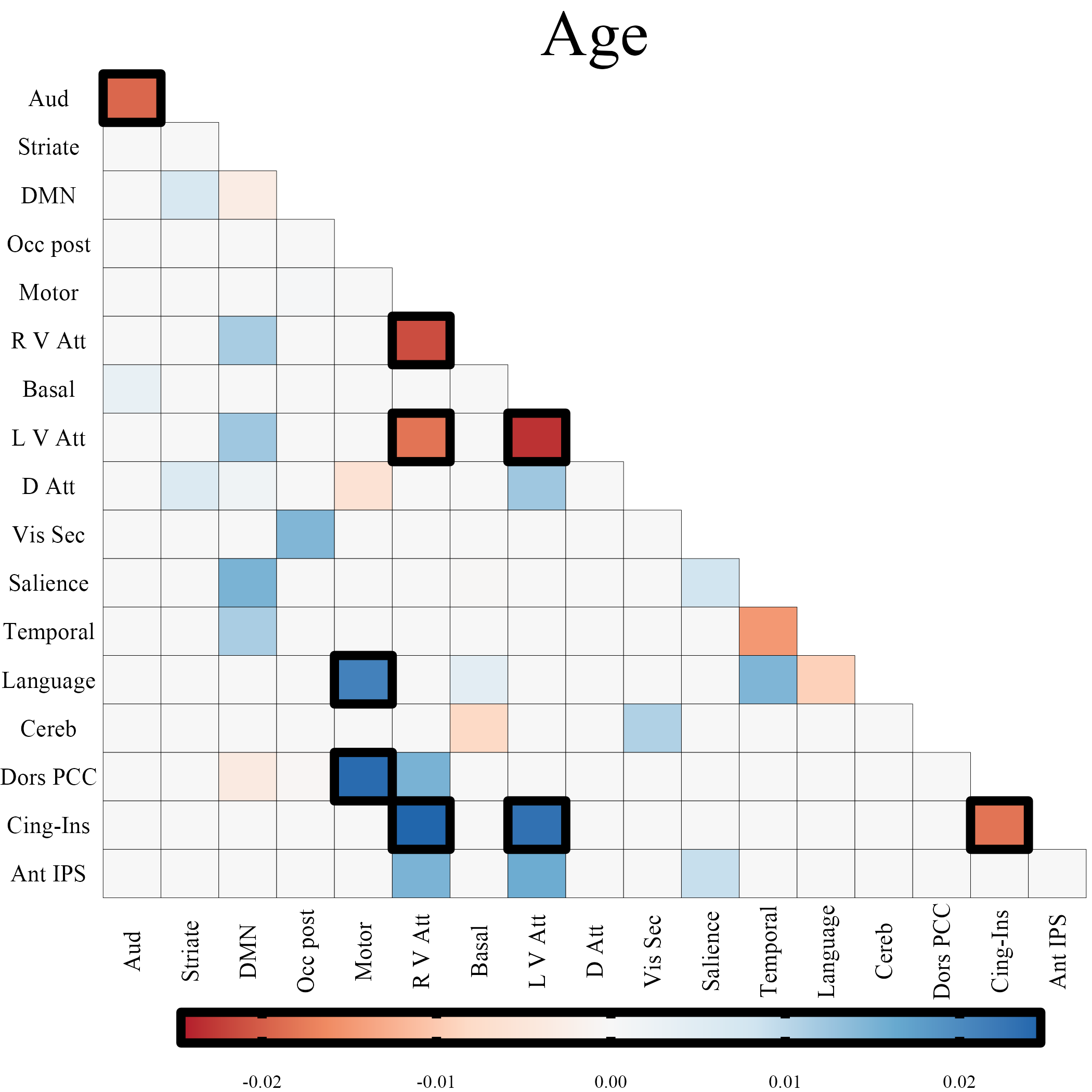
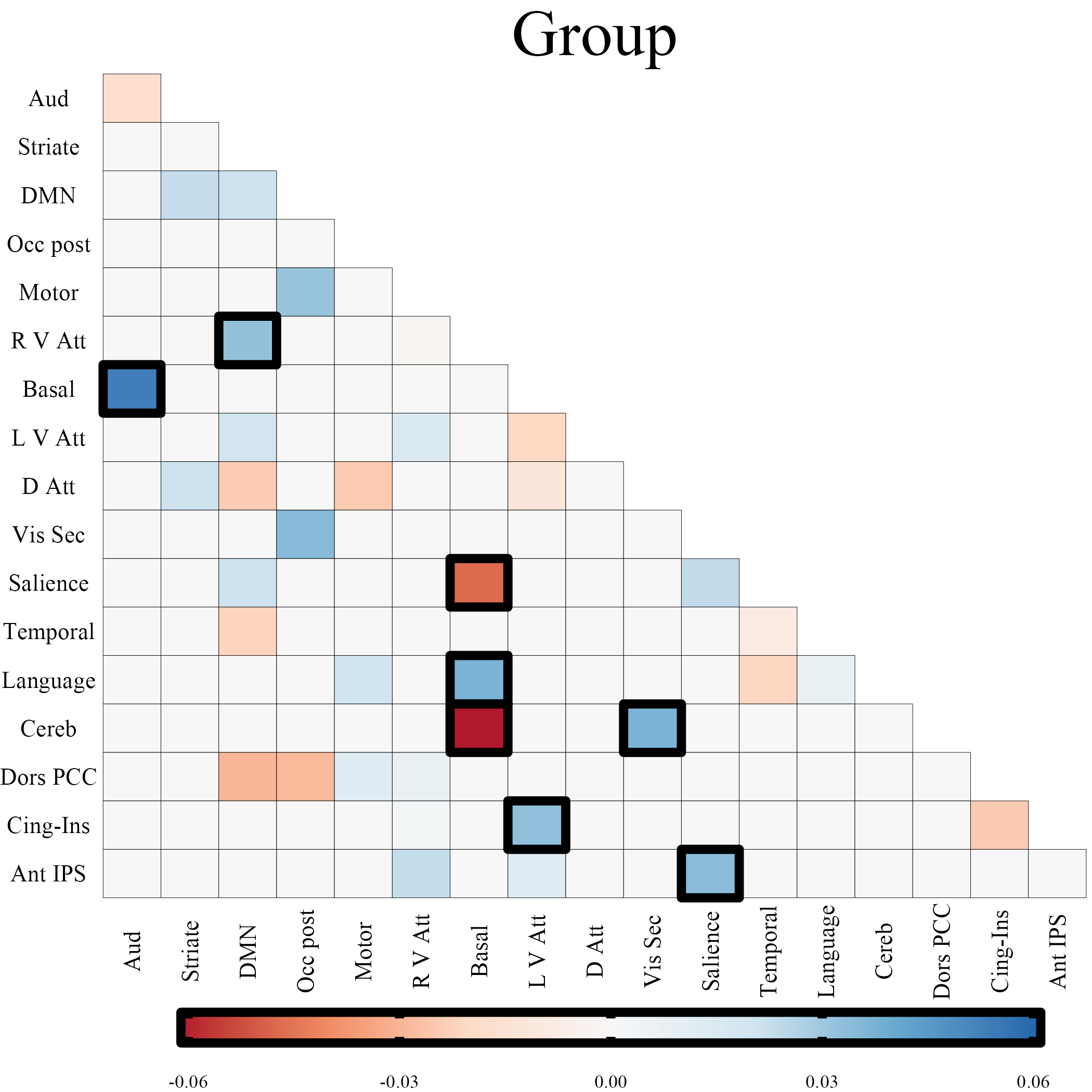
Figure 1:

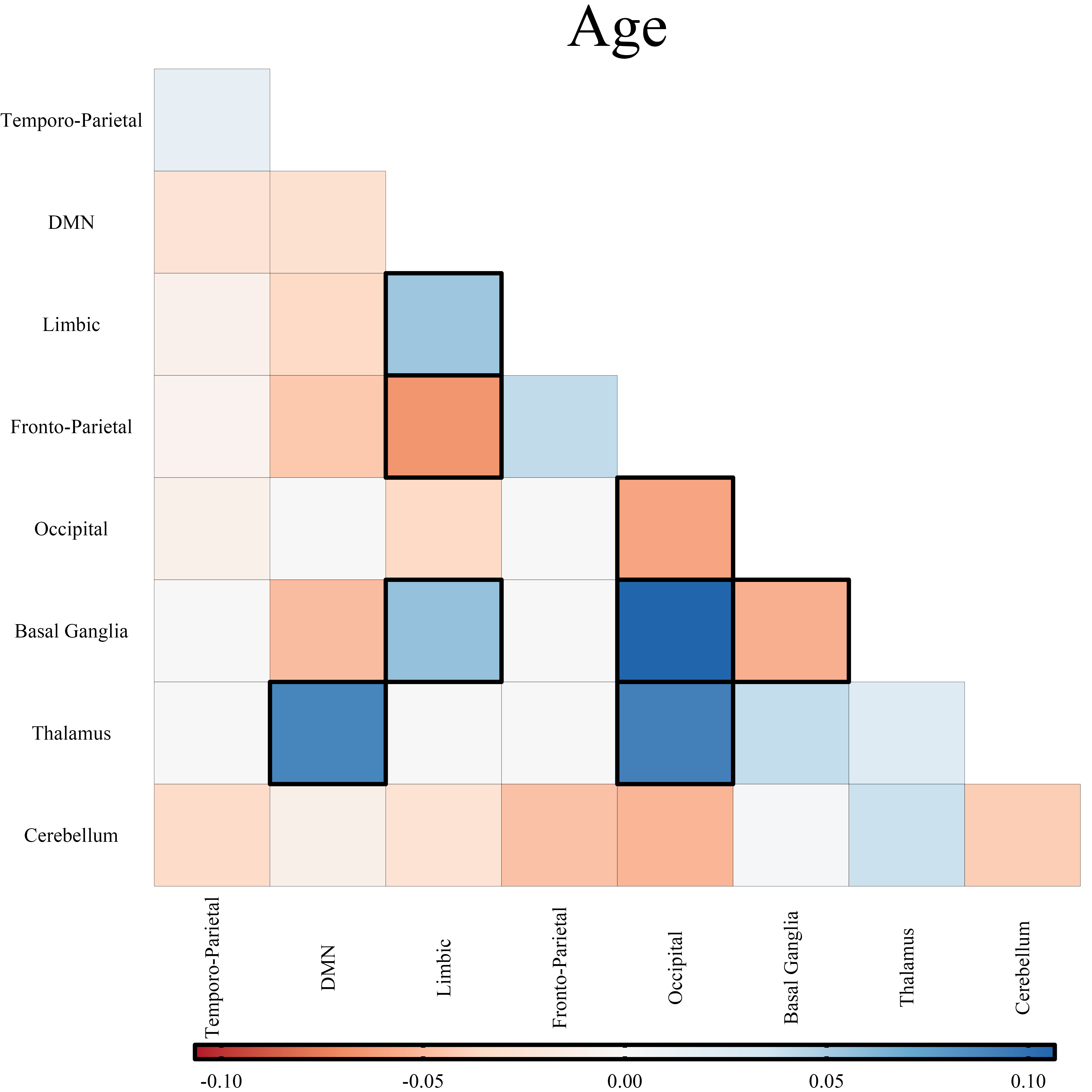
(a)

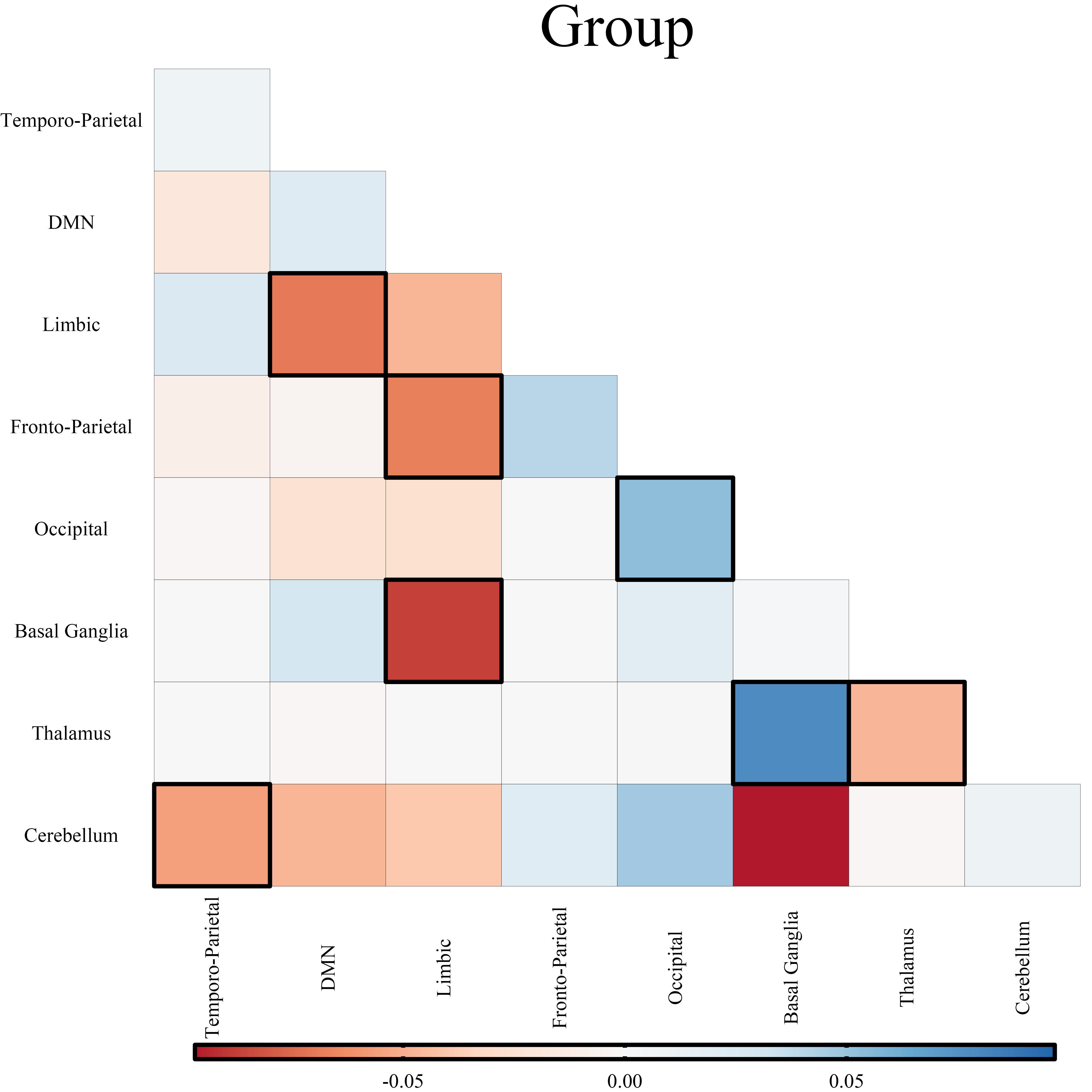
(b)

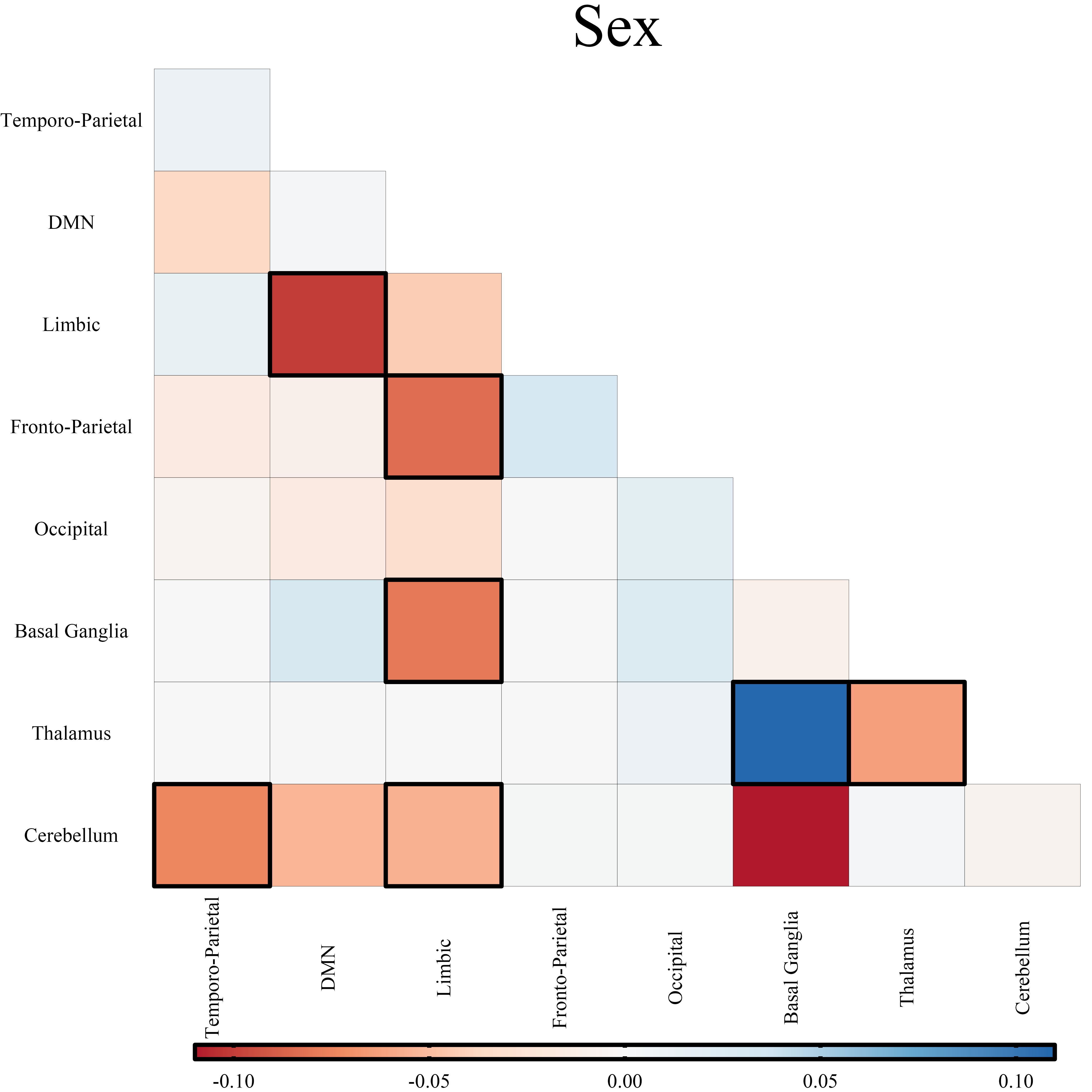
(c)

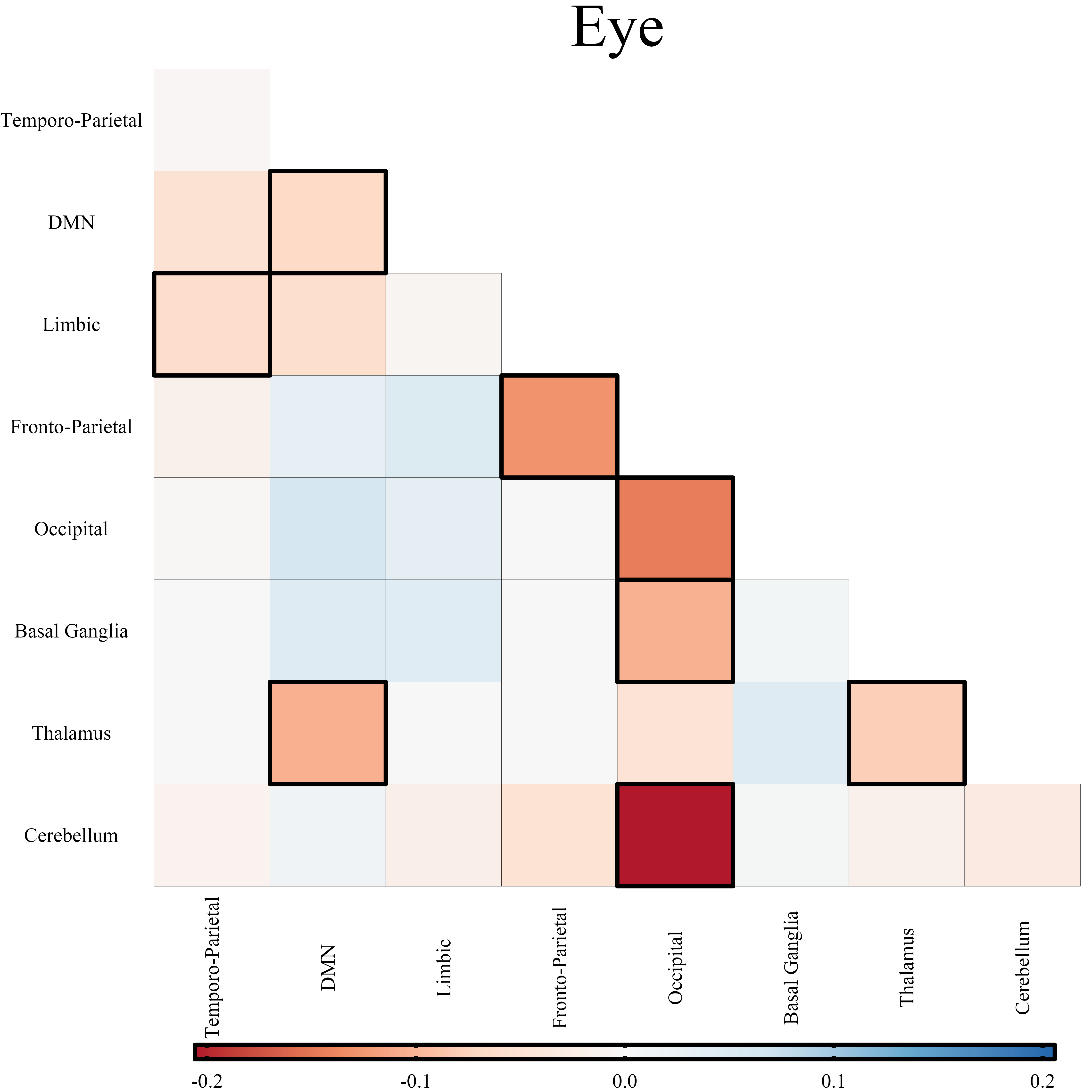
(d)

Figure 2:

Figure captions

1. Significant regression coefficients as measured by $\mathrm{VIP}$ for the R-PLS model on the COBRE dataset with $K=2$ latent variables, visualised as symmetric matrices. The regression coefficients have been averaged over the $17$ resting state networks of the MSDL atlas and show the coefficients for age (left) and subject group (right). The darker outlined boxes show the top $25\%$ influential regions as measured by the absolute coefficient value within and between each network.

2. Significant regression coefficients as measured by $\mathrm{VIP}$ for the R-PLS model on the ABIDE dataset with $K=3$ latent variables, visualised as symmetric matrices. The regression coefficients have been averaged over the $7$ resting state networks identified by Parente and Colosimo (2020)Parente2020 as well as the cerebellum network comprising the cerebellum and vermis. (a) shows the coefficients that predict age, (b) shows the coefficients that predict group, (c) shows the coefficients that predict sex, and (d) shows the coefficients that predict eye status. The darker outlined boxes show the top $25\%$ influential regions as measured by the absolute coefficient value within and between each network.

Tables

Table 1: Mean (SE) 10-fold cross validation results for R-PLS on the COBRE and ABIDE datasets, and Euclidean PLS using the raw and Fisher transformed correlations. The value $K$ represents the optimal number of latent variables for each model using the within one standard error rule. The full model metrics are the multivariate $R^{2}$ and RMSE. The group classification metrics look at the classification for subject group only. R-PLS is the best model for both datasets over all model metrics, except for specificity (bold values).

	Riemannian	Raw correlations	Fisher correlations
COBRE
K	2	3	3
Full model metrics (SE)
$R^{2}$	0.25 (0.035)	0.23 (0.033)	0.23 (0.036)
RMSE	1.20 (0.036)	1.21 (0.025)	1.21 (0.026)
Group classification (SE)
Accuracy	0.75 (0.045)	0.73 (0.032)	0.74 (0.032)
Sensitivity	0.81 (0.035)	0.70 (0.057)	0.72 (0.055)
Specificity	0.69 (0.071)	0.76 (0.048)	0.76 (0.048)
ABIDE
K	3	3	3
Full model metrics (SE)
$R^{2}$	0.15 (0.015)	0.07 (0.016)	0.07 (0.016)
RMSE	1.80 (0.051)	1.89 (0.059)	1.89 (0.059)
Group classification (SE)
Accuracy	0.58 (0.027)	0.55 (0.032)	0.54 (0.032)
Sensitivity	0.61 (0.058)	0.52 (0.064)	0.51 (0.063)
Specificity	0.53 (0.063)	0.58 (0.065)	0.58 (0.065)

Algorithms

Input: Data $X_{1},X_{2},\dots,X_{n}$, $Y_{1},Y_{2},\dots,Y_{n}$, Desired number of components $K$.

Output: PLS weights $\{\boldsymbol{w}_{k}\}_{k=1}^{K},\{\boldsymbol{c}_{k}\}_{k=1}^{K}$, Scores $\{\boldsymbol{t}_{k}\}_{k=1}^{K},\{\boldsymbol{u}_{k}\}_{k=1}^{K}$, Loadings $\{\boldsymbol{p}_{k}\}_{k=1}^{K}$, and Regression coefficients $\{\hat{\beta}_{1k}\}_{k=1}^{K}$.

1 Calculate Fréchet means $\mu_{X},\mu_{Y}$ (Algorithm S2^∗);

2 Linearise the data by;

3   $\boldsymbol{x}_{i}\leftarrow\operatorname{Log}_{\mu_{X}}{X_{i}}$;

4   $\boldsymbol{y}_{i}\leftarrow\operatorname{Log}_{\mu_{Y}}{Y_{i}}$;

5 Map $\boldsymbol{x}_{i}$, $\boldsymbol{y}_{i}$ to Euclidean space via coordinates $\phi$ on $T_{\mu_{X}}M$ and $\psi$ on $T_{\mu_{Y}}M$;

6 Perform NIPALS (Algorithm S1^∗) on $\{(\boldsymbol{x}_{i},\boldsymbol{y}_{i})\}$ to get weights $\{\boldsymbol{w}_{k}\}_{k=1}^{K},\{\boldsymbol{c}_{k}\}_{k=1}^{K}$, scores $\{\boldsymbol{t}_{k}\}_{k=1}^{K},\{\boldsymbol{u}_{k}\}_{k=1}^{K}$, loadings $\{\boldsymbol{p}_{k}\}_{k=1}^{K}$, and regression coefficients $\{\hat{\beta}_{1k}\}_{k=1}^{K}$;

Map $\boldsymbol{w}_{k},\boldsymbol{c}_{k}$ and $\boldsymbol{p}_{k}$ back to their appropriate tangent spaces using $\phi^{-1}$ and $\psi^{-1}$. ^∗Found in the supplementary material.

Algorithm 1 Tangent non-linear iterative partial least squares.

References

- (1) Contreras, J. A., Goñi, J., Risacher, S. L., Sporns, O. & Saykin, A. J. The structural and functional connectome and prediction of risk for cognitive impairment in older adults. \JournalTitleCurrent behavioral neuroscience reports 2, 234–245 (2015).
- (2) Yang, F. N., Liu, T. T. & Wang, Z. Functional connectome mediates the association between sleep disturbance and mental health in preadolescence: a longitudinal mediation study. \JournalTitleHuman Brain Mapping 43, 2041–2050 (2022).
- (3) Woodward, N. D. & Cascio, C. J. Resting-State Functional Connectivity in Psychiatric Disorders. \JournalTitleThe Journal of the American Medical Association Psychiatry 72, 743–744, DOI: 10.1001/JAMAPSYCHIATRY.2015.0484 (2015).
- (4) Shi, Y. & Toga, A. W. Connectome imaging for mapping human brain pathways. \JournalTitleMolecular psychiatry 22, 1230–1240 (2017).
- (5) Ogawa, S., Lee, T. M., Kay, A. R. & Tank, D. W. Brain magnetic resonance imaging with contrast dependent on blood oxygenation. \JournalTitleProceedings of the National Academy of Sciences of the United States of America 87, 9868–9872 (1990).
- (6) Wold, H. Soft Modelling by Latent Variables: The Non-Linear Iterative Partial Least Squares (NIPALS) Approach. \JournalTitleJournal of Applied Probability 12, 117–142, DOI: 10.1017/S0021900200047604 (1975).
- (7) McIntosh, A. R., Bookstein, F. L., Haxby, J. V. & Grady, C. L. Spatial Pattern Analysis of Functional Brain Images Using Partial Least Squares. \JournalTitleNeuroImage 3, 143–157, DOI: 10.1006/NIMG.1996.0016 (1996).
- (8) Krishnan, A., Williams, L. J., McIntosh, A. R. & Abdi, H. Partial Least Squares (PLS) methods for neuroimaging: A tutorial and review. \JournalTitleNeuroImage 56, 455–475, DOI: 10.1016/j.neuroimage.2010.07.034 (2011).
- (9) Pennec, X., Fillard, P. & Ayache, N. A Riemannian Framework for Tensor Computing. \JournalTitleInternational Journal of Computer Vision 66, 41–66, DOI: 10.1007/s11263-005-3222-z (2006).
- (10) Pennec, X., Sommer, S. & Fletcher, T. Riemannian Geometric Statistics in Medical Image Analysis (Elsevier, 2019).
- (11) Wong, E., Anderson, J. S., Zielinski, B. A. & Fletcher, P. T. Riemannian Regression and Classification Models of Brain Networks Applied to autism. \JournalTitleConnectomics in neuroImaging : second international workshop, CNI 2018, held in conjunction with MICCAI 2018, Granada, Spain, September 20, 2018 : proceedings. CNI (Workshop) (2nd : 2018 : Granada, Spain) 11083, 78, DOI: 10.1007/978-3-030-00755-3_9 (2018).
- (12) Chu, Y. et al. Decoding multiclass motor imagery EEG from the same upper limb by combining Riemannian geometry features and partial least squares regression. \JournalTitleJournal of Neural Engineering 17, 046029, DOI: 10.1088/1741-2552/ABA7CD (2020).
- (13) Zhang, C. & Liu, Q. Region Constraint Person Re-Identification via Partial Least Square on Riemannian Manifold. \JournalTitleIEEE Access 6, 17060–17066, DOI: 10.1109/ACCESS.2018.2808602 (2018).
- (14) Perez, R. A. & Gonzalez-Farias, G. Partial Least Squares Regression on Symmetric Positive-Definite Matrices. \JournalTitleRevista Colombiana de Estadistica 36, 177–192 (2013).
- (15) Wold, S., Johansson, E. & Cocchi, M. PLS: partial least squares projections to latent structures. \JournalTitle3D QSAR Drug Des 523–550 (1993).
- (16) Aine, C. J. et al. Multimodal Neuroimaging in Schizophrenia: Description and Dissemination. \JournalTitleNeuroinformatics 15, 343–364, DOI: 10.1007/s12021-017-9338-9 (2017).
- (17) Varoquaux, G., Baronnet, F., Kleinschmidt, A., Fillard, P. & Thirion, B. LNCS 6361 - Detection of Brain Functional-Connectivity Difference in Post-stroke Patients Using Group-Level Covariance Modeling (2010).
- (18) Craddock, C. et al. The Neuro Bureau Preprocessing Initiative: open sharing of preprocessed neuroimaging data and derivatives. \JournalTitleFrontiers in Neuroinformatics 7, DOI: 10.3389/CONF.FNINF.2013.09.00041/EVENT_ABSTRACT (2013).
- (19) Tzourio-Mazoyer, N. et al. Automated anatomical labeling of activations in SPM using a macroscopic anatomical parcellation of the MNI MRI single-subject brain. \JournalTitleNeuroImage 15, 273–289, DOI: 10.1006/nimg.2001.0978 (2002).
- (20) Varoquaux, G., Gramfort, A., Pedregosa, F., Michel, V. & Thirion, B. Multi-subject dictionary learning to segment an atlas of brain spontaneous activity. vol. 6801 LNCS, 562–573, DOI: 10.1007/978-3-642-22092-0_46 (Springer, 2011).
- (21) Parente, F. & Colosimo, A. Functional connections between and within brain subnetworks under resting-state. \JournalTitleScientific Reports 2020 10:1 10, 1–13, DOI: 10.1038/s41598-020-60406-7 (2020).
- (22) Varangis, E., Habeck, C. G., Razlighi, Q. R. & Stern, Y. The Effect of Aging on Resting State Connectivity of Predefined Networks in the Brain. \JournalTitleFrontiers in Aging Neuroscience 11, 234, DOI: 10.3389/FNAGI.2019.00234/BIBTEX (2019).
- (23) Edde, M., Leroux, G., Altena, E. & Chanraud, S. Functional brain connectivity changes across the human life span: From fetal development to old age. \JournalTitleJournal of Neuroscience Research 99, 236–262, DOI: 10.1002/JNR.24669 (2021).
- (24) Ferreira, L. K. et al. Aging Effects on Whole-Brain Functional Connectivity in Adults Free of Cognitive and Psychiatric Disorders. \JournalTitleCerebral Cortex 26, 3851–3865, DOI: 10.1093/CERCOR/BHV190 (2016).
- (25) Tomasi, D. & Volkow, N. D. Aging and functional brain networks. \JournalTitleMolecular Psychiatry 2012 17:5 17, 549–558, DOI: 10.1038/mp.2011.81 (2011).
- (26) Vidal-Piñiro, D. et al. Decreased Default Mode Network connectivity correlates with age-associated structural and cognitive changes. \JournalTitleFrontiers in Aging Neuroscience 6, 256, DOI: 10.3389/FNAGI.2014.00256/BIBTEX (2014).
- (27) Ramos, T. C., Balardin, J. B., Sato, J. R. & Fujita, A. Abnormal cortico-cerebellar functional connectivity in autism spectrum disorder. \JournalTitleFrontiers in systems neuroscience 12, 74 (2019).
- (28) Pascual-Belda, A., Díaz-Parra, A. & Moratal, D. Evaluating functional connectivity alterations in autism spectrum disorder using network-based statistics. \JournalTitleDiagnostics 8, 51 (2018).
- (29) Assaf, M. et al. Abnormal functional connectivity of default mode sub-networks in autism spectrum disorder patients. \JournalTitleNeuroImage 53, 247–256, DOI: 10.1016/J.NEUROIMAGE.2010.05.067 (2010).
- (30) Smith, R. E. et al. Sex differences in resting-state functional connectivity of the cerebellum in autism spectrum disorder. \JournalTitleFrontiers in Human Neuroscience 13, 104, DOI: 10.3389/FNHUM.2019.00104/BIBTEX (2019).
- (31) Zhang, B. et al. Altered Functional Connectivity of Striatum Based on the Integrated Connectivity Model in First-Episode Schizophrenia. \JournalTitleFrontiers in Psychiatry 10, 756, DOI: 10.3389/FPSYT.2019.00756/BIBTEX (2019).
- (32) Orliac, F. et al. Links among resting-state default-mode network, salience network, and symptomatology in schizophrenia. \JournalTitleSchizophrenia research 148, 74–80, DOI: 10.1016/J.SCHRES.2013.05.007 (2013).
- (33) Duan, M. et al. Altered basal ganglia network integration in schizophrenia. \JournalTitleFrontiers in Human Neuroscience 9, 561, DOI: 10.3389/FNHUM.2015.00561/BIBTEX (2015).
- (34) Karbasforoushan, H. & Woodward, N. Resting-state networks in schizophrenia. \JournalTitleCurrent topics in medicinal chemistry 12, 2404–2414, DOI: 10.2174/156802612805289863 (2012).
- (35) Woodward, N. D., Rogers, B. & Heckers, S. Functional resting-state networks are differentially affected in schizophrenia. \JournalTitleSchizophrenia Research 130, 86–93, DOI: 10.1016/J.SCHRES.2011.03.010 (2011).
- (36) Dong, D., Wang, Y., Chang, X., Luo, C. & Yao, D. Dysfunction of Large-Scale Brain Networks in Schizophrenia: A Meta-analysis of Resting-State Functional Connectivity. \JournalTitleSchizophrenia Bulletin 44, 168–181, DOI: 10.1093/SCHBUL/SBX034 (2018).
- (37) Yu, Q. et al. Brain connectivity networks in schizophrenia underlying resting state functional magnetic resonance imaging. \JournalTitleCurrent topics in medicinal chemistry 12, 2415, DOI: 10.2174/156802612805289890 (2012).
- (38) Wang, H. et al. Evidence of a dissociation pattern in default mode subnetwork functional connectivity in schizophrenia. \JournalTitleScientific reports 5, 14655 (2015).
- (39) Yan, C. et al. Spontaneous Brain Activity in the Default Mode Network Is Sensitive to Different Resting-State Conditions with Limited Cognitive Load. \JournalTitlePLOS ONE 4, e5743, DOI: 10.1371/JOURNAL.PONE.0005743 (2009).
- (40) Han, J. et al. Eyes-Open and Eyes-Closed Resting State Network Connectivity Differences. \JournalTitleBrain Sciences 13, 122 (2023).
- (41) Agcaoglu, O., Wilson, T. W., Wang, Y. P., Stephen, J. & Calhoun, V. D. Resting state connectivity differences in eyes open versus eyes closed conditions. \JournalTitleHuman Brain Mapping 40, 2488, DOI: 10.1002/HBM.24539 (2019).
- (42) Ryan, M. Riemannian statistical techniques with applications in fMRI. Ph.D. thesis, The University of Adelaide (2023).
- (43) Bellec, P. et al. A neuroimaging analyses kit for Matlab and Octave. 1–5 (Organization on Human Brain Mapping, 2011).
- (44) Behzadi, Y., Restom, K., Liau, J. & Liu, T. T. A component based noise correction method (CompCor) for BOLD and perfusion based fMRI. \JournalTitleNeuroImage 37, 90–101, DOI: 10.1016/j.neuroimage.2007.04.042 (2007).
- (45) Nguyen, D. V. & Rocke, D. M. Tumor classification by partial least squares using microarray gene expression data. \JournalTitleBioinformatics 18, 39–50, DOI: 10.1093/BIOINFORMATICS/18.1.39 (2002).
- (46) Hulland, J. Use of partial least squares (PLS) in strategic management research: A review of four recent studies. \JournalTitleStrategic Management Journal 20, 195–204, DOI: 10.1002/(SICI)1097-0266(199902)20:2 (1999).
- (47) McIntosh, A. R. & Lobaugh, N. J. Partial least squares analysis of neuroimaging data: applications and advances. \JournalTitleNeuroImage 23, S250–S263, DOI: 10.1016/J.NEUROIMAGE.2004.07.020 (2004).
- (48) Lin, F. H. et al. Multivariate analysis of neuronal interactions in the generalized partial least squares framework: simulations and empirical studies. \JournalTitleNeuroImage 20, 625–642, DOI: 10.1016/S1053-8119(03)00333-1 (2003).
- (49) Rosipal, R. & Krämer, N. Overview and Recent Advances in Partial Least Squares. \JournalTitleLecture Notes in Computer Science (including subseries Lecture Notes in Artificial Intelligence and Lecture Notes in Bioinformatics) 3940 LNCS, 34–51, DOI: 10.1007/11752790_2 (2006).
- (50) Garthwaite, P. H. An interpretation of partial least squares. \JournalTitleJournal of the American Statistical Association 89, 122–127, DOI: 10.1080/01621459.1994.10476452 (1994).
- (51) Geladi, P. & Kowalski, B. R. Partial least-squares regression: a tutorial. \JournalTitleAnalytica Chimica Acta 185, 1–17, DOI: 10.1016/0003-2670(86)80028-9 (1986).
- (52) Höskuldsson, A. PLS regression methods. \JournalTitleJournal of Chemometrics 2, 211–228, DOI: 10.1002/CEM.1180020306 (1988).
- (53) Tenenhaus, M. La régression PLS: Théorie et pratique (Technip, 1998).
- (54) Tran, T. N., Afanador, N. L., Buydens, L. M. & Blanchet, L. Interpretation of variable importance in Partial Least Squares with Significance Multivariate Correlation (sMC). \JournalTitleChemometrics and Intelligent Laboratory Systems 138, 153–160, DOI: 10.1016/J.CHEMOLAB.2014.08.005 (2014).
- (55) Galindo-Prieto, B., Eriksson, L. & Trygg, J. Variable influence on projection (VIP) for orthogonal projections to latent structures (OPLS). \JournalTitleJournal of Chemometrics 28, 623–632, DOI: 10.1002/cem.2627 (2014).
- (56) Afanador, N. L., Tran, T. N. & Buydens, L. M. Use of the bootstrap and permutation methods for a more robust variable importance in the projection metric for partial least squares regression. \JournalTitleAnalytica Chimica Acta 768, 49–56, DOI: 10.1016/J.ACA.2013.01.004 (2013).
- (57) Benjamini, Y. & Hochberg, Y. Controlling the False Discovery Rate: A Practical and Powerful Approach to Multiple Testing. \JournalTitleJournal of the Royal Statistical Society: Series B (Methodological) 57, 289–300, DOI: 10.1111/j.2517-6161.1995.tb02031.x (1995).
- (58) Lee, J. M. Introduction to Topological Manifolds, vol. 202 (Springer New York, 2011).
- (59) Lee, J. M. Introduction to Smooth Manifolds, vol. 218 (Springer New York, 2012).
- (60) Lee, J. M. Introduction to Riemannian Manifolds, vol. 176 (Springer International Publishing, 2018).
- (61) do Carmo, M. P. Riemannian Geometry (Birkhauser Boston Inc, 1992).
- (62) Fréchet, M. Les éléments aléatoires de nature quelconque dans un espace distancié. \JournalTitleAnnales de l’institut Henri Poincaré 10, 215–310 (1948).
- (63) Kim, H. J. et al. Canonical Correlation Analysis on Riemannian Manifolds and Its Applications. 251–267, DOI: 10.1007/978-3-319-10605-2_17 (Springer, 2014).
- (64) Fletcher, P. T. Geodesic regression and the theory of least squares on Riemannian manifolds. \JournalTitleInternational Journal of Computer Vision 105, 171–185, DOI: 10.1007/s11263-012-0591-y (2013).
- (65) Venkatesh, M., Jaja, J. & Pessoa, L. Comparing functional connectivity matrices: A geometry-aware approach applied to participant identification. \JournalTitleNeuroImage 207, 116398, DOI: 10.1016/j.neuroimage.2019.116398 (2020).
- (66) Hastie, T., Tibshirani, R. & Friedman, J. The Elements of Statistical Learning (Springer New York, 2009).
- (67) R Core Team. R: A Language and Environment for Statistical Computing (2022).
Acknowledgements
M.R. acknowledges the Australian Government Research Training Program Scholarship that funded this research.