Adaptive sieving: A dimension reduction technique for sparse optimization problems

Abstract

In this paper, we propose an adaptive sieving (AS) strategy for solving general sparse machine learning models by effectively exploring the intrinsic sparsity of the solutions, wherein only a sequence of reduced problems with much smaller sizes need to be solved. We further apply the proposed AS strategy to generate solution paths for large-scale sparse optimization problems efficiently. We establish the theoretical guarantees for the proposed AS strategy including its finite termination property. Extensive numerical experiments are presented in this paper to demonstrate the effectiveness and flexibility of the AS strategy to solve large-scale machine learning models.

Keywords: Adaptive sieving, dimension reduction, sparse optimization problems
AMS subject classification: 90C06, 90C25, 90C90

1 Introduction

Consider the convex composite optimization problems of the following form:

$$\min_{x\in\mathbb{R}^{n}}\ \displaystyle\Big{\{}\Phi(x)+P(x)\Big{\}},$$ (1)

where $\Phi:\mathbb{R}^{n}\rightarrow\mathbb{R}$ is a convex twice continuously differentiable function and $P:\mathbb{R}^{n}\to(-\infty,+\infty]$ is a closed and proper convex function. The optimization problems in this form cover a wide class of models in modern data science applications and statistical learning. In practice, the regularizer $P(\cdot)$ is usually chosen to enforce sparsity with desirable structure in the estimators obtained from the model, especially in high-dimensional cases. For example, the Lasso regularizer [24] is proposed to force element-wise sparsity in the predictors, and the group lasso regularizer [30] is proposed to impose group-wise sparsity. Moreover, many more complicated regularizers have also been proposed to study other structured sparsity, such as the sparse group lasso regularizer [8, 13], the Sorted L-One Penalized Estimation (SLOPE) [3] and the exclusive lasso regularizer [34, 15].

Currently, many popular first-order methods have been proposed to solve the problems in the form of (1), such as the accelerated proximal gradient (APG) method [1], the alternating direction method of multipliers (ADMM) [7, 11] and the block coordinate descent (BCD) method [26, 12, 23]. Each algorithm is designed to solve only a highly specialized subset of large-scale optimization problems having a specific structure that is conducive for the method to carry out low-cost computations in each iteration. These algorithms are especially popular in machine learning and statistics in recent years. However, first-order methods are often not robust and generally are only able to deliver low accuracy solutions. More recently, the highly efficient and robust second-order algorithms based on the augmented Lagrangian method have achieved increasing attention for solving important classes of large-scale structured convex programming problems in the form of (1), including those involving the Lasso regularizer [17], the sparse group lasso regularizer [33], the SLOPE [20] and the exclusive lasso regularizer [18].

However, both the first-order and second-order algorithms for solving the problems in the form of (1) are often susceptible to the curse of dimensionality [2]. Fortunately, the desired solutions to the model in practice are usually highly sparse, where the nonzero entries correspond to selected features. Inspired by this property, in this paper, we propose an adaptive sieving strategy for solving sparse optimization models in the form of (1), by sieving out a large proportion of inactive features to significantly reduce the dimension of the problems, which can then highly accelerate the computation. The proposed AS strategy does not depend on the specific form of the regularizer $P(\cdot)$, as long as the proximal mapping of $P(\cdot)$ can be computed in an efficient way. It is worth emphasizing that our AS strategy can be applied to any solver providing that it is able to solve the reduced problems to the required accuracy. Numerical experiments demonstrate that our AS strategy is very effective in reducing the problem dimensions and accelerating the computation for solving sparse optimization models.

We will then apply the proposed AS strategy to generate solution paths for large-scale machine learning models, which is necessary for model selection via cross-validation in practice. In particular, we are interested in solving the following problem for a sequence of values of the parameter $\lambda$:

$$\min_{x\in\mathbb{R}^{n}}\ \displaystyle\Big{\{}\Phi(x)+\lambda P(x)\Big{\}}. P_{\lambda}$$ ()

Here the hyper-parameter $\lambda>0$ is added to control the trade-off between the loss and the sparsity level of the solutions. To reduce the computation time of obtaining a solution path, especially for high-dimensional cases, various feature screening rules, which attempt to drop some inactive features based on prior analysis, have been proposed. Tibshirani et al. [25] proposed a strong screening rule (SSR) based on the “unit-slope” bound assumption for the Lasso model and the regression problem with the elastic net regularizer. This idea has been extended to the SLOPE model recently [16]. Compared to this unsafe screening rule where some active features may be screened out by mistake, safe screening rules have been extensively studied. The first safe screening rule was proposed by El Ghaoui et al. [10] for Lasso models. Later on, Wang et al. [28, 27] proposed a dual polytope projection based screening rule (DPP) and an enhanced version (EDPP) for Lasso and group lasso models via carefully analyzing the geometry of the corresponding dual problems. Other safe screening rules, like Sphere test [29], have been proposed via different strategies for estimating compact regions containing the optimal solutions to the dual problems. The safe screening rules will not exclude active features, but in many instances they only exclude a small subset of inactive features due to their conservative nature. In addition, the safe screening rules are usually not applicable to generate a solution path for a sequence of the hyperparameters with large gaps. Recently, Zeng et al. [32] combined the SSR and the EDPP to propose a hybrid safe-strong screening rule, which was implemented in an R package biglasso [31]. However, these screening rules are usually problem specific and they are difficult to be applied to the models with general regularizers, like the exclusive lasso regularizer, as they are highly dependent on the separability and positive homogeneity of the regularizers. Also, they implicitly require the reduced problems to be solved exactly.

Based on our proposed AS strategy for solving the problem (1), we design a path generation method for generating solution paths of the machine learning model ($P_{\lambda}$), wherein a sequence of reduced problems with much smaller sizes need to be solved. Our path generation method exhibits great improvement over the existing screening rules in three aspects. First, it applies to the models with general regularizers, including those are non-separable or not positively homogeneous. Second, it does not require the reduced problems to be solved exactly. Third, as we will see in the numerical experiments, it is more aggressive, and is able to sieve out more inactive features. Here, it is worth mentioning that, the aforementioned screening rules are only for generating the solution path and they cannot be applied directly for solving a single problem with a fixed parameter.

The remaining part of the paper is organized as follows. In Section 2, we propose the adaptive sieving strategy for solving the sparse optimization models in the form of (1), followed by its theoretical analysis including the finite termination property in Section 3. In Section 4, we will design a path generation method for general sparse optimization models based on the proposed AS strategy. Section 5 provides the numerical performance of the proposed AS strategy for solving various machine learning models on both synthetic data and real data. Experiments are also conducted to demonstrate the superior performance of the path generation method based on the AS strategy compared to other popular screening rules. Finally, we conclude the paper.

Notations: Denote the set $[n]=\{1,2,\cdots,n\}$. For any $I\subseteq[n]$, $\overline{I}$ denotes the complement of $I$ in $[n]$. For any $z\in\mathbb{R}$, ${\rm sign}(z)$ denotes the sign function of $z$. For any $x\in\mathbb{R}^{n}$, denotes its $p$-norm as $\|x\|_{p}=(\sum_{i=1}^{p}|x_{i}|^{p})^{1/p}$. For simplicity, we denote $\|\cdot\|=\|\cdot\|_{2}$. For any vector $x\in\mathbb{R}^{n}$ and any index set $I\subseteq[n]$, denote $x_{I}$ as the subvector generated by the elements of $x$ indexed by $I$. For any closed and proper convex function $q:\mathbb{R}^{n}\rightarrow(-\infty,\infty]$, the proximal mapping of $q(\cdot)$ is defined by

$${\rm Prox}_{q}(x):=\underset{y\in\mathbb{R}^{n}}{\arg\min}\ \Big{\{}q(y)+\frac{1}{2}\|y-x\|^{2}\Big{\}},$$ (2)

for any $x\in\mathbb{R}^{n}$. It is known that ${\rm Prox}_{q}(\cdot)$ is Lipschitz continuous with modulus $1$ [22].

2 Dimension reduction via adaptive sieving

Throughout this paper, we make the following blanket assumption, which is satisfied for many popular machine learning models, as discussed in [35, Section 2.1].

Assumption 1.

Assume that the solution set of (1), denoted as $\Omega$, is nonempty and compact.

2.1 The adaptive sieving strategy

We propose an adaptive sieving strategy for solving sparse optimization models in the form of (1). An appealing property of this strategy is that it does not depend on the specific form of the regularizer and thus can be applied to sparse optimization problems with general regularization functions. More importantly, due to the adaptive nature of the AS strategy, it can sieve out a very large proportion of inactive features to significantly reduce the dimension of the problems and accelerate the computation by a large margin. This further shows that the AS strategy actually serves as a powerful dimension reduction technique for sparse optimization models.

Algorithm 1 An adaptive sieving strategy for solving (1)

1:  Input: an initial index set $I^{0}\subseteq[n]$, a given tolerance $\epsilon\geq 0$ and a given positive integer $k_{\max}$ (e.g., $k_{\max}=500$).

2:  Output: an approximate solution $x^{*}$ to the problem (1) satisfying $\|R(x^{*})\|\leq\epsilon$.

3:  1. Find

$$x^{0}\in\underset{x\in\mathbb{R}^{n}}{\arg\min}\ \Big{\{}\Phi(x)+P(x)-\langle\delta^{0},x\rangle\ \mid\ x_{\overline{I^{0}}}=0\Big{\}},$$ (3)

where $\delta^{0}\in\mathbb{R}^{n}$ is an error vector such that $\|\delta^{0}\|\leq\epsilon$ and $(\delta^{0})_{\overline{I^{0}}}=0$. 2. Compute $R(x^{0})$ and set $s=0$.

4:  while $\|R(x^{s})\|>\epsilon$ do

5:     3.1. Create $J^{s+1}$ as

$$J^{s+1}=\Big{\{}j\in\overline{I^{s}}\;\mid\;(R(x^{s}))_{j}\neq 0\Big{\}}.$$ (4)

If $J^{s+1}=\emptyset$, let $I^{s+1}\leftarrow I^{s}$; otherwise, let $k$ be a positive integer satisfying $k\leq\min\{|J^{s+1}|,k_{\max}\}$ and define

$$\widehat{J}^{s+1}=\Big{\{}j\in J^{s+1}~{}|~{}\mbox{ $|(R(x^{s}))_{j}|$ is among the first $k$ largest values in $\{|(R(x^{s}))_{i}|\}_{i\in J^{s+1}}$ }\Big{\}}.$$

Update $I^{s+1}$ as:

$$I^{s+1}\leftarrow I^{s}\cup\widehat{J}^{s+1}.$$

6:     3.2. Solve the constrained problem:

$$x^{s+1}\in\underset{x\in\mathbb{R}^{n}}{\arg\min}\ \Big{\{}\Phi(x)+P(x)-\langle\delta^{s+1},x\rangle\ \mid\ x_{\overline{I^{s+1}}}=0\Big{\}},$$ (5)

where $\delta^{s+1}\in\mathbb{R}^{n}$ is an error vector such that $\|\delta^{s+1}\|\leq\epsilon$ and $(\delta^{s+1})_{\overline{I^{s+1}}}=0$.

7:     3.3: Compute $R(x^{s+1})$ and set $s\leftarrow s+1$.

8:  end while

9:  return: Set $x^{*}=x^{s}$.

We give the details of the AS strategy in Algorithm 1. Here in order to measure the accuracy of the approximate solutions, we define the proximal residual function $R:\mathbb{R}^{n}\rightarrow\mathbb{R}^{n}$ associated with the problem (1) as

$$R(x):=x-{\rm Prox}_{P}(x-\nabla\Phi(x)),\quad x\in\mathbb{R}^{n}.$$ (6)

The KKT condition of (1) implies that $\bar{x}\in\Omega$ if and only if $R(\bar{x})=0$.

A few remarks of Algorithm 1 are in order. First, in Algorithm 1, the introduction of the error vectors $\delta^{0}$, $\{\delta^{s+1}\}$ in (3) and (5) implies that the corresponding minimization problems can be solved inexactly. It is important to emphasize that the vectors are not a priori given but they are the errors incurred when the original problems (with $\delta^{0}=0$ in (3) and $\delta^{s+1}=0$ in (5)) are solved inexactly. We will explain how the error vectors $\delta^{0}$, $\{\delta^{s+1}\}$ in (3) and (5) can be obtained in Section 3. Second, the initial active feature index set $I^{0}$ is suggested to be chosen such that $|I^{0}|\ll n$, in consideration of the computational cost. Third, the sizes of the reduced problems (3) and (5) are usually much smaller than $n$, which will be demonstrated in the numerical experiments.

We take the least squares linear regression problem as an example to show an efficient initialization of the index set $I^{0}$ via the correlation test, which is similar to the idea of the surely independent screening rule in [9]. Consider $\Phi(x)=\frac{1}{2}\|Ax-b\|^{2}$, where $A=[a_{1},a_{2},\cdots,a_{n}]\in\mathbb{R}^{m\times n}$ is a given feature matrix, $b\in\mathbb{R}^{m}$ is a given response vector. One can choose $k\lceil\sqrt{n}\rceil$ initial active features based on the correlation test between each feature vector $a_{i}$ and the response vector $b$. That is, one can compute $s_{i}:=|\langle a_{i},b\rangle|/(\|a_{i}\|\|b\|)$ for $i=1,\cdots,n$, and choose the initial guess of $I^{0}$ as

$$I^{0}=\left\{i\in[n]:s_{i}\mbox{ is among the first }k\lceil\sqrt{n}\rceil\mbox{ largest values in}\;s_{1},\ldots,s_{n}\right\}.$$

In practice, we usually choose $k=10$.

2.2 Examples of the regularizer

As we shall see in Algorithm 1, there is no restriction on the form of the regularizer $P(\cdot)$. In particular, it is not necessary to be separable or positively homogeneous, which is an important generalization compared to the existing screening rules [25, 10, 28, 27, 29, 32, 31]. The only requirement for $P(\cdot)$ is that its proximal mapping ${\rm Prox}_{P}(\cdot)$ can be computed in an efficient way. Fortunately, it is the case for almost all popular regularizers used in practice. Below, We list some examples of the regularizers for better illustration.

• Lasso regularizer [24]:

  $$P(x)=\lambda\|x\|_{1},\quad x\in\mathbb{R}^{n},$$

  where $\lambda>0$ is a given parameter.

• Elastic net regularizer [36]:

  $$P(x)=\lambda_{1}\|x\|_{1}+\lambda_{2}\|x\|^{2},\quad x\in\mathbb{R}^{n},$$

  where $\lambda_{1},\lambda_{2}>0$ are given parameters.

• Sparse group lasso regularizer [8, 13]:

  $$P(x)=\lambda_{1}\|x\|_{1}+\lambda_{2}\sum_{l=1}^{g}w_{l}\|x_{G_{l}}\|,\quad x\in\mathbb{R}^{n},$$

  where $\lambda_{1},\lambda_{2}>0$, $w_{1},\cdots,w_{g}\geq 0$ are parameters, and $\{G_{1},\cdots,G_{g}\}$ is a disjoint partition of the set $[n]$. For the limiting case when $\lambda_{1}=0$, we get the group lasso regularizer [30].

• Exclusive lasso regularizer [34, 15]:

  $$P(x)=\lambda\sum_{l=1}^{g}\|w_{G_{l}}\circ x_{G_{l}}\|_{1}^{2},\quad x\in\mathbb{R}^{n},$$

  where $\lambda>0$ is a given parameter, $w\in\mathbb{R}^{n}_{++}$ is a weight vector and $\{G_{1},\cdots,G_{g}\}$ is a disjoint partition of the index set $[n]$.

• Sorted L-One Penalized Estimation (SLOPE) [3]:

  $$P(x)=\sum_{i=1}^{n}\lambda_{i}|x|_{(i)},$$

  with parameters $\lambda_{1}\geq\cdots\geq\lambda_{n}\geq 0$ and $\lambda_{1}>0$. For a given vector $x\in\mathbb{R}^{n}$, we denote $|x|$ to be the vector in $\mathbb{R}^{n}$ obtained from $x$ by taking the absolute value of its components. We define $|x|_{(i)}$ to be the $i$-th largest component of $|x|$ such that $|x|_{(1)}\geq\cdots\geq|x|_{(n)}$.

Among the above examples, the screening rules of the Lasso regularizer and the group lasso regularizer have been intensively studied in [25, 10, 28, 27, 29, 32, 31]. Recently, a strong screening rule has been proposed for SLOPE [16]. However, no unified approach has been proposed for sparse optimization problems with general regularizers. Fortunately, our proposed AS strategy is applicable to all the above examples, which includes three different kinds of “challenging” regularizers. In particular, 1) the sparse group lasso regularizer is a combination of two regularizers; 2) the SLOPE is not separable; 3) the exclusive lasso regularizer is not positively homogeneous.

3 Theoretical analysis of the AS strategy

In this section, we provide the theoretical analysis of the proposed AS strategy for solving sparse optimization problems presented in Algorithm 1. An appealing advantage of our proposed AS strategy is that it allows the involved reduced problems to be solved inexactly due to the introduction of the error vectors $\delta^{0}$, $\{\delta^{s+1}\}$ in (3) and (5). It is important to emphasize that the vectors are not a priori given but they are the errors incurred when the original problems (with $\delta^{0}=0$ in (3) and $\delta^{s+1}=0$ in (5)) are solved inexactly. The following proposition explains how the error vectors $\delta^{0}$, $\{\delta^{s+1}\}$ in (3) and (5) can be obtained.

Proposition 1.

Given any $s=0,1,\cdots$. The updating rule of $x^{s}$ in Algorithm 1 can be interpreted in the procedure as follows. Let $M_{s}$ be a linear map from $\mathbb{R}^{|I^{s}|}$ to $\mathbb{R}^{n}$ defined as

$$(M_{s}z)_{I^{s}}=z,\quad(M_{s}z)_{\overline{I^{s}}}=0,\quad z\in\mathbb{R}^{|I^{s}|},$$

and $\Phi^{s}$, $P^{s}$ be functions from $\mathbb{R}^{|I^{s}|}$ to $\mathbb{R}$ defined as $\Phi^{s}(z):=\Phi(M_{s}z)$, $P^{s}(z):=P(M_{s}z)$ for all $z\in\mathbb{R}^{|I^{s}|}$. Then $x^{s}\in\mathbb{R}^{n}$ can be computed as

$$(x^{s})_{I^{s}}:={\rm Prox}_{P^{s}}(\hat{z}-\nabla\Phi^{s}(\hat{z})),$$

and $(x^{s})_{\overline{I^{s}}}=0$, where $\hat{z}$ is an approximate solution to the problem

$$\min_{z\in\mathbb{R}^{|I^{s}|}}\ \Big{\{}\Phi^{s}(z)+P^{s}(z)\Big{\}},$$ (7)

which satisfies

$$\|\hat{z}-{\rm Prox}_{P^{s}}(\hat{z}-\nabla\Phi^{s}(\hat{z}))+\nabla\Phi^{s}({\rm Prox}_{P^{s}}(\hat{z}-\nabla\Phi^{s}(\hat{z})))-\nabla\Phi^{s}(\hat{z})\|\leq\epsilon,$$ (8)

where $\epsilon$ is the parameter given in Algorithm 1.

If the function $\Phi(\cdot)$ is $L$-smooth, that is, it is continuously differentiable and its gradient is Lipschitz continuous with constant $L$:

$$\|\nabla\Phi(x)-\nabla\Phi(y)\|\leq L\|x-y\|,\quad\forall x,y\in\mathbb{R}^{n},$$

then the condition (8) can be achieved by

$$\|\hat{z}-{\rm Prox}_{P^{s}}(\hat{z}-\nabla\Phi^{s}(\hat{z}))\|\leq\frac{\epsilon}{1+L}.$$

Proof.

Let $\{z^{i}\}$ be a sequence that converges to a solution of the problem (7). For any $i=1,2,\cdots$, define $\varepsilon^{i}:=z^{i}-{\rm Prox}_{P^{s}}(z^{i}-\nabla\Phi^{s}(z^{i}))+\nabla\Phi^{s}({\rm Prox}_{P^{s}}(z^{i}-\nabla\Phi^{s}(z^{i})))-\nabla\Phi^{s}(z^{i})$. By the continuous differentiability of $\Phi^{s}(\cdot)$ and [6, Lemma 4.5], we know that $\lim_{i\rightarrow\infty}\|\varepsilon^{i}\|=0$, which implies the existence of $\hat{z}$ in (8).

Next we explain the reason why the updating rule of $x^{s}$ in Algorithm 1 can be interpreted as the one stated in the proposition. Since $(x^{s})_{I^{s}}:={\rm Prox}_{P^{s}}(\hat{z}-\nabla\Phi^{s}(\hat{z}))$, we have

$$\hat{z}-(x^{s})_{I^{s}}-\nabla\Phi^{s}(\hat{z})\in\partial P^{s}((x^{s})_{I^{s}}).$$

If we choose $\hat{\delta}:=\hat{z}-(x^{s})_{I^{s}}+\nabla\Phi^{s}((x^{s})_{I^{s}})-\nabla\Phi^{s}(\hat{z})\in\mathbb{R}^{|I^{s}|}$, then we have

$$\hat{\delta}\in\nabla\Phi^{s}((x^{s})_{I^{s}})+\partial P^{s}((x^{s})_{I^{s}}),$$

which means that $x^{s}$ is the exact solution to the problem

$$\min_{x\in\mathbb{R}^{n}}\ \Big{\{}\Phi(x)+P(x)-\langle\delta^{s},x\rangle\ \mid\ x_{\overline{I^{s}}}=0\Big{\}},$$

with $\delta^{s}:=M_{s}\hat{\delta}$. Moreover, we can see that $(\delta^{s})_{\overline{I^{s}}}=(M_{s}\hat{\delta})_{\overline{I^{s}}}=0$ and

$$\|\delta^{s}\|=\|\hat{\delta}\|=\|\hat{z}-(x^{s})_{I^{s}}+\nabla\Phi^{s}((x^{s})_{I^{s}})-\nabla\Phi^{s}(\hat{z})\|\leq\epsilon.$$

If $\Phi(\cdot)$ is $L$-smooth, we have that

$$\|\hat{\delta}\| =\|\hat{z}-(x^{s})_{I^{s}}+\nabla\Phi^{s}((x^{s})_{I^{s}})-\nabla\Phi^{s}(\hat{z})\|$$

$$\leq\|\hat{z}-(x^{s})_{I^{s}}\|+\|\nabla\Phi^{s}((x^{s})_{I^{s}})-\nabla\Phi^{s}(\hat{z})\|$$

$$=\|\hat{z}-(x^{s})_{I^{s}}\|+\|M_{s}^{T}\nabla\Phi(M_{s}(x^{s})_{I^{s}})-M_{s}^{T}\nabla\Phi(M_{s}\hat{z})\|$$

$$\leq\|\hat{z}-(x^{s})_{I^{s}}\|+\|\nabla\Phi(M_{s}(x^{s})_{I^{s}})-\nabla\Phi(M_{s}\hat{z})\|$$

$$\leq\|\hat{z}-(x^{s})_{I^{s}}\|+L\|M_{s}(x^{s})_{I^{s}}-M_{s}\hat{z}\|$$

$$=(1+L)\|\hat{z}-(x^{s})_{I^{s}}\|,$$

which means that (8) can be achieved by

$$\|\hat{z}-{\rm Prox}_{P^{s}}(\hat{z}-\nabla\Phi^{s}(\hat{z}))\|\leq\frac{\epsilon}{1+L}.$$

This completes the proof. ∎

Next, we will show the convergence properties of Algorithm 1 in the following proposition, which states that the algorithm will terminate after a finite number of iterations.

Theorem 1.

The while loop in Algorithm 1 will terminate after a finite number of iterations.

Proof.

We first prove that when $\|R(x^{s})\|>\epsilon\geq 0$ for some $s\geq 0$, the index set $J^{s+1}$ defined in (4) is nonempty. We prove this by contradiction. Suppose that $J^{s+1}=\emptyset$, which means

$$(R(x^{s}))_{\overline{I^{s}}}=0.$$

According to the definition of $R(\cdot)$ in (6), we have

$$R(x^{s})-\nabla\Phi(x^{s})\in\partial P(x^{s}-R(x^{s})).$$

Note that $x^{s}$ satisfies

$$x^{s}\in\underset{x\in\mathbb{R}^{n}}{\arg\min}\ \Big{\{}\Phi(x)+P(x)-\langle\delta^{s},x\rangle\ \mid\ x_{\overline{I^{s}}}=0\Big{\}},$$

where $\delta^{s}\in\mathbb{R}^{n}$ is an error vector such that $(\delta^{s})_{\overline{I^{s}}}=0$ and $\|\delta^{s}\|\leq\epsilon$. By the KKT condition of the above minimization problem, we know that there exists a multiplier $y\in\mathbb{R}^{n}$ with $y_{I^{s}}=0$ such that

$$\left\{\begin{aligned} &0\in\nabla\Phi(x^{s})+\partial P(x^{s})-\delta^{s}-y,\\ &\Big{(}x^{s}\Big{)}_{\overline{I^{s}}}=0,\end{aligned}\right.$$

which means

$$\delta^{s}+y-\nabla\Phi(x^{s})\in\partial P(x^{s}).$$

By the maximal monotonicity of the operator $\partial P$, we have

$$\langle R(x^{s})-\delta^{s}-y,-R(x^{s})\rangle\geq 0,$$

which implies that

$$\|R(x^{s})\|^{2}\leq\langle\delta^{s}+y,R(x^{s})\rangle=\langle(\delta^{s})_{I^{s}},(R(x^{s}))_{I^{s}}\rangle\leq\|\delta^{s}\|\|R(x^{s})\|\leq\epsilon\|R(x^{s})\|.$$

Thus, we get $\|R(x^{s})\|\leq\epsilon$, which is a contradiction.

Therefore, we have that for any $s\geq 0$, $J^{s+1}\neq\emptyset$ as long as $R(x^{s})>\epsilon$, which further implies that $\widehat{J}^{s+1}\neq\emptyset$. In other words, new indices will be added to the index set $I^{s+1}$ as long as the KKT residual has not achieved at the required accuracy. Since the total number of features $n$ is finite, the while loop in Algorithm 1 will terminate after a finite number of iterations. ∎

Although we only have the finite termination guarantee for the proposed AS strategy, the superior empirical performance of the AS strategy will be demonstrated later in Section 5 with extensive numerical experiments. In particular, the number of AS iterations is no more than 5 (less than 3 for most of the cases) for solving a single sparse optimization problem in our experiments on both synthetic and real datasets.

4 An efficient path generation method based on the AS strategy

When solving machine learning models in practice, we need to solve the model with a sequence of hyper-parameters and then select appropriate values for the hyper-parameters based on some methodologies, such as cross-validation. In this section, we are going to propose a path generation method based on the AS strategy to obtain solution paths of general sparse optimization models. Specifically, we will borrow the idea of the proposed AS strategy to solve the model ($P_{\lambda}$) for a sequence of $\lambda$ in a highly efficient way.

Before presenting our path generation method, we first briefly discuss the ideas behind the two most popular screening rules for obtaining solution paths of various machine learning models, namely the strong screening rule (SSR) [25] and the dual polytope projection based screening rule (DPP) [28, 27]. For convenience, we take the Lasso model as an illustration, with $\Phi(x)=\frac{1}{2}\|Ax-b\|^{2}$ and $P(x)=\|x\|_{1}$ in ($P_{\lambda}$), where $A=[a_{1},a_{2},\cdots,a_{n}]\in\mathbb{R}^{m\times n}$ is the feature matrix and $b\in\mathbb{R}^{m}$ is the response vector. Let $x^{*}(\lambda)$ be an optimal solution to ($P_{\lambda}$). The KKT condition implies that:

$$a_{i}^{T}\theta^{*}(\lambda)\in\left\{\begin{array}[]{ll}\{\lambda\ {\rm sign}(x^{*}(\lambda))\}&\mbox{if}\;x^{*}(\lambda)_{i}\not=0\\ \left[-\lambda,\lambda\right]&\mbox{if}\;x^{*}(\lambda)_{i}=0\\ \end{array}\right.,$$

where $\theta^{*}(\lambda)$ is the optimal solution of the associated dual problem:

$$\max_{\theta\in\mathbb{R}^{m}}\ \Big{\{}\frac{1}{2}\|b\|^{2}-\frac{1}{2}\|\theta-b\|^{2}\;\mid\;|a_{i}^{T}\theta|\leq\lambda,\ i=1,2,\dots,n\Big{\}}.$$ (9)

The existing screening rules for the Lasso model are based on the fact that $x^{*}(\lambda)_{i}=0$ if $|a_{i}^{T}\theta^{*}(\lambda)|<\lambda$. The difference is how to estimate $a_{i}^{T}\theta^{*}(\lambda)$ based on an optimal solution $x^{*}(\tilde{\lambda})$ of $({\rm P}_{\tilde{\lambda}})$ for some $\tilde{\lambda}>\lambda$, without solving the dual problem (9). The SSR [25] discards the $i$-th predictor if

$$|a_{i}^{T}\theta^{*}(\tilde{\lambda})|\leq 2\lambda-\tilde{\lambda},$$

by assuming the “unit slope” bound condition: $|a_{i}^{T}\theta^{*}(\lambda_{1})-a_{i}^{T}\theta^{*}(\lambda_{2})|\leq|\lambda_{1}-\lambda_{2}|$, for all $\lambda_{1},\lambda_{2}>0$. Since this assumption may fail, the SSR may screen out some active features by mistake. Also, the SSR only works for consecutive hyper-parameters with a small gap, since it requires $\lambda>\frac{\tilde{\lambda}}{2}$. Wang et al. [28, 27] proposed the DPP by carefully analysing the properties of the optimal solution to the dual problem (9). The key idea is, if we can estimate a region $\Theta_{\lambda}$ containing $\theta^{*}(\lambda)$, then

$$\sup_{\theta\in\Theta_{\lambda}}|a_{i}^{T}\theta|<\lambda\quad\Longrightarrow\quad x^{*}(\lambda)_{i}=0.$$

They estimate the region $\Theta_{\lambda}$ by realizing that the optimal solution of (9) is the projection onto a polytope. As we can see, a tighter estimation of $\Theta_{\lambda}$ will induce a better safe screening rule.

The bottlenecks of applying the above screening rules to solve general machine learning models in the form of (1) are: 1) the subdifferential of a general regularizer may be much more complicated than the Lasso regularizer, whose subdifferential is separable; 2) a general regularizer may not be positively homogeneous, which means that the optimal solution to the dual problem may not be the projection onto some convex set [21, Theorem 13.2]; 3) These screening rules may only exclude a small portion of zeros in practice even if the solutions of the problem are highly sparse, thus we still need to solve large-scale problems after the screening; 4) they implicitly require the reduced problems to be solved exactly, which is unrealistic for many machine learning models in practice.

To overcome these challenges, we propose a path generation method based on the AS strategy for solving the problem ($P_{\lambda}$) presented in Algorithm 2. Here we denote the proximal residual function $R_{\lambda}:\mathbb{R}^{n}\rightarrow\mathbb{R}^{n}$ associated with ($P_{\lambda}$) as

$$R_{\lambda}(x):=x-{\rm Prox}_{\lambda P}(x-\nabla\Phi(x)),\quad x\in\mathbb{R}^{n}.$$ (10)

Assume that for any $\lambda>0$, the solution set of ($P_{\lambda}$) is nonempty and compact.

Algorithm 2 An AS-based path generation method for ($P_{\lambda}$)

1:  Input: a sequence of hyper-parameters: $\lambda_{0}>\lambda_{1}>\dots>\lambda_{k}>0$, and given tolerances $\epsilon\geq 0$ and $\hat{\epsilon}\geq 0$.

2:  Output: a solution path: $x^{*}(\lambda_{0}),x^{*}(\lambda_{1}),x^{*}(\lambda_{2}),\dots,x^{*}(\lambda_{k})$.

3:  1. Apply Algorithm 1 to solve the problem $(\mbox{P}_{\lambda_{0}})$ with the tolerance $\epsilon$, and then denote the output as $x^{*}(\lambda_{0})$. Let

$$I^{*}(\lambda_{0}):=\{j\;\mid\;|x^{*}(\lambda_{0})_{j}|>\hat{\epsilon},\ j=1,\cdots,n\}.$$

4:  for $i=1,2,\dots,k$ do

5:     2.1. Let $I^{0}(\lambda_{i})=I^{*}(\lambda_{i-1})$.

6:     2.2. Apply Algorithm 1 to solve the problem $(\mbox{P}_{\lambda_{i}})$ with the initial index set $I^{0}(\lambda_{i})$ and the tolerance $\epsilon$. Denote the output as $x^{*}(\lambda_{i})$.

7:     2.3. Let

$$I^{*}(\lambda_{i}):=\{j\;\mid\;|x^{*}(\lambda_{i})_{j}|>\hat{\epsilon},\ j=1,\cdots,n\}.$$

8:  end for

The design of the above algorithm directly leads us to the following theorem regarding its convergence property. The proof of the theorem can be obtained directly due to Theorem 1.

Theorem 2.

The solution path $x^{*}(\lambda_{0}),x^{*}(\lambda_{1}),\dots,x^{*}(\lambda_{k})$ generated by Algorithm 2 forms a sequence of approximate solutions to the problems $(\mbox{P}_{\lambda_{0}}),(\mbox{P}_{\lambda_{1}}),\cdots,(\mbox{P}_{\lambda_{k}})$, in the sense that

$$\|R_{\lambda_{i}}(x^{*}(\lambda_{i}))\|\leq\epsilon,\quad i=0,1,\cdots,k.$$

In practice, we usually choose $\hat{\epsilon}=10^{-10}$. We will compare the numerical performance of the proposed AS strategy to the popular screening rules in Section 5, our experiment results will show that the AS strategy is much more efficient for solving large-scale sparse optimization problems.

5 Numerical Experiments

In this section, we will present extensive numerical results to demonstrate the performance of the AS strategy. We will test the performance of the AS strategy on the sparse optimization problems of the following form:

$$\min_{x\in\mathbb{R}^{n}}\ \Big{\{}h(Ax)+\lambda P(x)\Big{\}},$$ (11)

where $A:\mathbb{R}^{n}\to\mathbb{R}^{m}$ is a given data matrix, $h:\mathbb{R}^{m}\to\mathbb{R}$ is a twice continuously differentiable loss function, $P:\mathbb{R}^{n}\to(-\infty,+\infty]$ is a proper closed convex regularization function, and $\lambda>0$ is the hyper-parameter. More specifically, we consider the following two most commonly used loss functions for $h(\cdot)$:

• (linear regression) $h(y)=\sum_{i=1}^{m}(y_{i}-b_{i})^{2}/2$, for some given vector $b\in\mathbb{R}^{m}$;

• (logistic regression) $h(y)=\sum_{i=1}^{m}\log(1+\exp(-b_{i}y_{i}))$, for some given vector $b\in\{-1,1\}^{m}$.

For the regularization function $P(\cdot)$, we consider four important regularizers in statistical learning models: lasso, sparse group lasso, exclusive lasso, and SLOPE. Details of the regularizers can be found in Section 2.2. The algorithms used for solving each sparse optimization model and its corresponding reduced problems when applying the AS strategy will be specified later in the related subsections.

In our experiments, we measure the accuracy of the obtained solution by the relative KKT residual:

$$\eta_{\rm KKT}:=\frac{\|x-{\rm Prox}_{\lambda P}(x-A^{T}\nabla h(Ax)\|}{1+\|x\|+\|A^{T}\nabla h(Ax)\|}.$$

We terminate the tested algorithm when $\eta_{\rm KKT}\leq\varepsilon$, where $\varepsilon>0$ is a given tolerance, which is set to be $10^{-6}$ by default. We choose $\hat{\epsilon}=10^{-10}$ in Algorithm 2. We set the maximum running time for solving each individual problem on the solution path to be $30$ minutes for all solvers used later in this section. All our numerical results are obtained by running MATLAB(2022a version) on a Windows workstation (Intel Xeon E5-2680 @2.50GHz).

The numerical experiments will be organized as follows. First, we will present the numerical performance of the AS strategy on the mentioned models on synthetic data sets in Section 5.1 and Section 5.2. Second, we will present the numerical results on nine real data sets in Section 5.3. To further demonstrate the superior performance of the AS strategy, we will compare it with other popular feature screening rules in Section 5.4.

5.1 Performance of the AS strategy for linear regression on synthetic data

In this subsection, we conduct numerical experiments to demonstrate the performance of the AS strategy for linear regression on synthetic data. In order to better illustrate the effect of the AS in the numerical results, we will use Sieving_round to represent the total number of the AS rounds during the path generation, and use Avg_dim (Max_dim) to denote the average (maximum) dimension of the reduced problems on the solution path generated by the AS strategy.

We first describe the generation of the synthetic data sets. We consider the models with group structure (e.g., sparse group lasso and exclusive lasso) and without group structure (e.g., Lasso and SLOPE). For simplicity, we randomly generate data with groups and test all the models on these data. Motivated by [4], we generate the synthetic data using the model $b=Ax^{*}+\xi$, where $x^{*}$ is the predefined true solution and $\xi\sim\mathcal{N}(0,I_{m})$ is a random noise vector. Given the number of observations $m$, the number of groups $g$ and the number of features $p$ in each group, we generate each row of the matrix $A\in\mathbb{R}^{m\times gp}$ by independently sampling a vector from a multivariate normal distribution $\mathcal{N}(0,\Sigma)$, where $\Sigma$ is a Toeplitz covariance matrix with entries $\Sigma_{ij}=0.9^{|i-j|}$ for the features in the same group, and $\Sigma_{ij}=0.3^{|i-j|}$ for the features in different groups. For the ground-truth $x^{*}$, we randomly generate $r$ nonzero elements in each group with i.i.d values drawn from the uniform distribution on $[0,10]$. In particular, we test for $r\in\{\lfloor 0.1\%\times p\rfloor,\lfloor 1\%\times p\rfloor\}$.

Here, we mainly focus on solving the regression models in high-dimensional settings. In our experiments, we set $m\in\{500,1000,2000\}$. For the number of features, for simplicity, we fix $g$ to be $20$, but vary the number of features $p$ in each group from $5000$ to $60000$. That is, we vary the total number of features $n=gp$ from $100000$ to $1200000$.

5.1.1 Numerical results on Lasso linear regression problems

In this subsection, we present the numerical results of the Lasso linear regression model. We will apply the state-of-the-art semismooth Newton based augmented Lagrangian (SSNAL) method [17] to solve the Lasso model and its corresponding reduced problems generated by the AS strategy. The comparison of the efficiency between the SSNAL method and other popular algorithms for solving Lasso models can be found in [17]. Following the numerical experiment settings in [17], we test the numerical performance of the AS strategy for generating a solution path for the Lasso linear regression model with $\lambda=\lambda_{c}\|A^{T}b\|_{\infty}$, where $\lambda_{c}$ is taken from $10^{-1}$ to $10^{-4}$ with 20 equally divided grid points on the $\log_{10}$ scale.

Table 1: Numerical performance of the AS strategy applied to the generation of solution paths for the Lasso linear regression model on synthetic data sets with sparsity level $0.1\%$.

		Total time (hh:mm:ss)	Information of the AS
$m$	$n(=g\times p)$	Warmstart $|$ With AS	Sieving_round	Avg_dim $|$ Max_dim
$500$	$100,000$	00:00:32 $|$ 00:00:08	30	665 $|$ 3312
	$200,000$	00:01:01 $|$ 00:00:08	28	761 $|$ 4523
	$600,000$	00:02:56 $|$ 00:00:09	23	842 $|$ 7766
	$1,200,000$	00:08:14 $|$ 00:00:12	21	1018 $|$ 10954
$1000$	$100,000$	00:01:31 $|$ 00:00:19	33	1087 $|$ 3783
	$200,000$	00:03:01 $|$ 00:00:26	28	1344 $|$ 5308
	$600,000$	00:09:30 $|$ 00:00:32	30	1551 $|$ 7914
	$1,200,000$	00:17:39 $|$ 00:00:37	25	1681 $|$ 11037
$2000$	$100,000$	00:02:45 $|$ 00:01:27	36	1715 $|$ 3347
	$200,000$	00:05:07 $|$ 00:01:49	37	2076 $|$ 5847
	$600,000$	00:13:03 $|$ 00:02:25	33	2542 $|$ 9341
	$1,200,000$	00:24:59 $|$ 00:02:47	32	2744 $|$ 11610

We show the numerical results in Tables 1-2, where the performance of the AS strategy and the well-known warm-start technique for generating solution paths of Lasso linear regression problems are compared with different sparsity levels $r$ and different problem sizes $(m,n)$. From the numerical results, we can see that the AS strategy can effectively reduce the dimension of the optimization problems. Moreover, from the running time perspective, the AS strategy can accelerate the SSNAL method up to $\mathbf{43}$ times for generating solution paths for the Lasso linear regression model.

Table 2: Numerical performance of the AS strategy applied to the generation of solution paths for the Lasso linear regression model on synthetic data sets with sparsity level $1\%$.

		Total time (hh:mm:ss)	Information of the AS
$m$	$n(=g\times p)$	Warmstart $|$ With AS	Sieving_round	Avg_dim $|$ Max_dim
$500$	$100,000$	00:00:53 $|$ 00:00:07	31	682 $|$ 3310
	$200,000$	00:01:14 $|$ 00:00:07	26	765 $|$ 4503
	$600,000$	00:04:49 $|$ 00:00:09	25	830 $|$ 7760
	$1,200,000$	00:08:46 $|$ 00:00:12	23	997 $|$ 10956
$1000$	$100,000$	00:01:17 $|$ 00:00:25	29	1304 $|$ 4958
	$200,000$	00:02:28 $|$ 00:00:27	29	1345 $|$ 5180
	$600,000$	00:07:03 $|$ 00:00:34	31	1554 $|$ 7898
	$1,200,000$	00:12:55 $|$ 00:00:38	27	1644 $|$ 11035
$2000$	$100,000$	00:03:20 $|$ 00:02:14	33	2372 $|$ 11074
	$200,000$	00:05:04 $|$ 00:02:17	34	2574 $|$ 11172
	$600,000$	00:13:27 $|$ 00:02:22	32	2557 $|$ 9357
	$1,200,000$	00:25:30 $|$ 00:02:39	31	2773 $|$ 11757

5.1.2 Numerical results on exclusive lasso linear regression problems

In this subsection, we present the numerical results of the exclusive lasso linear regression model.

Table 3: Numerical performance of the AS strategy applied to the generation of solution paths for the exclusive lasso linear regression model on synthetic data sets with sparsity level $0.1\%$.

		Total time (hh:mm:ss)	Information of the AS
$m$	$n(=g\times p)$	Warmstart $|$ With AS	Sieving_round	Avg_dim $|$ Max_dim
$500$	$100,000$	00:00:34 $|$ 00:00:07	32	225 $|$ 3161
	$200,000$	00:01:05 $|$ 00:00:08	32	268 $|$ 4471
	$600,000$	00:03:10 $|$ 00:00:11	30	330 $|$ 7751
	$1,200,000$	00:06:57 $|$ 00:00:16	28	386 $|$ 10951
$1000$	$100,000$	00:01:06 $|$ 00:00:12	28	208 $|$ 3161
	$200,000$	00:01:58 $|$ 00:00:16	30	310 $|$ 4471
	$600,000$	00:05:19 $|$ 00:00:23	30	341 $|$ 7751
	$1,200,000$	00:10:44 $|$ 00:00:30	29	417 $|$ 10951
$2000$	$100,000$	00:01:33 $|$ 00:00:24	22	146 $|$ 3161
	$200,000$	00:02:53 $|$ 00:00:28	20	236 $|$ 4471
	$600,000$	00:09:11 $|$ 00:00:50	27	381 $|$ 7751
	$1,200,000$	00:19:28 $|$ 00:01:03	26	441 $|$ 10951

We apply the state-of-the-art dual Newton based proximal point algorithm (PPDNA) [18] to solve the exclusive lasso model and its corresponding reduced problems generated by the AS strategy. The comparison of the efficiency between the PPDNA and other popular algorithms for solving exclusive lasso models can be found in [18]. We follow the numerical experiment settings in [18] and test the numerical performance of generating a solution path for the exclusive lasso regression model with $\lambda=\lambda_{c}\|A^{T}b\|_{\infty}$ and $w$ being the vector of all ones. Here, $\lambda_{c}$ is taken from $10^{-1}$ to $10^{-4}$ with 20 equally divided grid points on the $\log_{10}$ scale.

We summarize the numerical results in Tables 3-4. We can see that the AS strategy gives excellent performance when generating solution paths for the exclusive lasso linear regression problems, in the sense that it highly reduces the dimension of the optimization problems and also accelerates the PPDNA algorithm up to 30 times.

Table 4: Numerical performance of the AS strategy applied to the generation of solution paths for the exclusive lasso linear regression model on synthetic data sets with sparsity level $1\%$.

		Total time (hh:mm:ss)	Information of the AS
$m$	$n(=g\times p)$	Warmstart $|$ With AS	Sieving_round	Avg_dim $|$ Max_dim
$500$	$100,000$	00:00:34 $|$ 00:00:05	29	199 $|$ 3161
	$200,000$	00:01:09 $|$ 00:00:05	30	206 $|$ 4471
	$600,000$	00:03:06 $|$ 00:00:08	24	284 $|$ 7751
	$1,200,000$	00:07:03 $|$ 00:00:14	22	343 $|$ 10951
$1000$	$100,000$	00:00:49 $|$ 00:00:10	29	213 $|$ 3161
	$200,000$	00:01:37 $|$ 00:00:12	31	234 $|$ 4471
	$600,000$	00:04:19 $|$ 00:00:17	22	298 $|$ 7751
	$1,200,000$	00:08:18 $|$ 00:00:23	21	348 $|$ 10951
$2000$	$100,000$	00:01:35 $|$ 00:00:26	25	196 $|$ 3161
	$200,000$	00:02:54 $|$ 00:00:29	25	241 $|$ 4471
	$600,000$	00:08:04 $|$ 00:00:35	23	302 $|$ 7751
	$1,200,000$	00:16:02 $|$ 00:00:50	22	356 $|$ 10951

5.1.3 Numerical results on sparse group lasso linear regression problems

In this subsection, we present the numerical results on the sparse group lasso linear regression model. We are going to apply the state-of-the-art SSNAL method [33] to solve the sparse group lasso model and its corresponding reduced problems generated by the AS strategy during the path generation. The comparison of the efficiency and robustness between the SSNAL method and other popular algorithms for solving sparse group lasso models is presented in [33].

Following the settings in [33], we test the numerical performance of the AS strategy for generating a solution path for the sparse group lasso linear regression model with $w_{l}=\sqrt{|G_{l}|}$ for each $l=1,\cdots,g$. For the parameters $\lambda_{1}$ and $\lambda_{2}$ in the sparse group lasso regularizer, we take $\lambda_{1}=\lambda_{c}\|A^{T}b\|_{\infty}$, $\lambda_{2}=\lambda_{1}/w_{\max}$ with $w_{\max}=\max\{w_{1},\dots,w_{g}\}$. Here, $\lambda_{c}$ is taken from $10^{-1}$ to $10^{-4}$ with 20 equally divided grid points on the $\log_{10}$ scale.

We summarize the numerical results of the comparison of the AS strategy and the warm-start technique for generating solution paths of sparse group lasso linear regression problems in Tables 5-6. As we can see from the tables, the AS strategy significantly accelerates the path generation of the sparse group lasso linear regression models. For example, on the synthetic data set of size $(m,n)=(2000,1200000)$ with sparsity level $1\%$ in Table 6, generating a solution path of the sparse group lasso problem with the warm-start technique takes around $2$ hours, while with our proposed AS strategy, it only takes less than $6$ minutes. The superior performance of the AS strategy can also been seen from the much smaller sizes of the reduced problems compared with the original problem sizes.

Table 5: Numerical performance of the AS strategy applied to the generation of solution paths for the sparse group lasso linear regression model on synthetic data sets with sparsity level $0.1\%$.

		Total time (hh:mm:ss)	Information of the AS
$m$	$n(=g\times p)$	Warmstart $|$ With AS	Sieving_round	Avg_dim $|$ Max_dim
$500$	$100,000$	00:03:00 $|$ 00:00:35	17	1743 $|$ 3588
	$200,000$	00:04:58 $|$ 00:00:38	16	2234 $|$ 4829
	$600,000$	00:14:11 $|$ 00:00:55	21	2764 $|$ 7839
	$1,200,000$	00:27:34 $|$ 00:01:00	20	3215 $|$ 10998
$1000$	$100,000$	00:05:47 $|$ 00:02:36	22	2000 $|$ 4259
	$200,000$	00:10:28 $|$ 00:02:16	19	2827 $|$ 6295
	$600,000$	00:31:02 $|$ 00:02:16	17	3570 $|$ 8311
	$1,200,000$	00:52:40 $|$ 00:02:21	16	4286 $|$ 11252
$2000$	$100,000$	00:15:46 $|$ 00:06:19	34	2062 $|$ 3464
	$200,000$	00:23:18 $|$ 00:06:46	33	3006 $|$ 6321
	$600,000$	00:58:03 $|$ 00:05:31	25	4742 $|$ 11063
	$1,200,000$	01:55:24 $|$ 00:07:07	26	5327 $|$ 12557

Table 6: Numerical performance of the AS strategy applied to the generation of solution paths for the sparse group lasso linear regression model on synthetic data sets with sparsity level $1\%$.

		Total time (hh:mm:ss)	Information of the AS
$m$	$n(=g\times p)$	Warmstart $|$ With AS	Sieving_round	Avg_dim $|$ Max_dim
$500$	$100,000$	00:02:46 $|$ 00:00:35	19	1993 $|$ 3783
	$200,000$	00:04:54 $|$ 00:00:33	15	2277 $|$ 4757
	$600,000$	00:13:28 $|$ 00:00:40	15	2864 $|$ 7842
	$1,200,000$	00:32:21 $|$ 00:00:51	16	3154 $|$ 11000
$1000$	$100,000$	00:05:59 $|$ 00:01:58	16	2684 $|$ 6558
	$200,000$	00:10:30 $|$ 00:02:08	19	3001 $|$ 6532
	$600,000$	00:27:42 $|$ 00:02:06	16	3578 $|$ 8196
	$1,200,000$	00:54:15 $|$ 00:02:12	16	4115 $|$ 11206
$2000$	$100,000$	00:14:06 $|$ 00:05:34	25	4078 $|$ 12657
	$200,000$	00:23:27 $|$ 00:05:27	23	4615 $|$ 13895
	$600,000$	01:03:53 $|$ 00:06:08	26	5035 $|$ 11284
	$1,200,000$	01:55:16 $|$ 00:05:28	19	5476 $|$ 12693

5.1.4 Numerical results on SLOPE linear regression problems

Here, we present the results on SLOPE linear regression model. We will apply the state-of-the-art SSNAL method [20] to solve the SLOPE regression model and its corresponding reduced problems generated by the AS strategy. The comparison of the efficiency between the SSNAL method and other popular algorithms for solving SLOPE models can be found in [20]. For the weights $\lambda_{(i)}$ in the SLOPE model, we follow the experiment settings in [3]. We test the numerical performance on generating a solution path for the SLOPE regression model with $\lambda=\lambda_{c}\|A^{T}b\|_{\infty}$, where $\lambda_{c}$ is taken from $10^{-1}$ to $10^{-4}$ with 20 equally divided grid points on the $\log_{10}$ scale.

The results are presented in Tables 7-8. We again observe the superior performance of the AS strategy on solving sparse optimization models. Specifically, when we apply the warm-start technique to generate solution paths for the SLOPE linear regression model with $(m,n)=(2000,1200000)$, it runs out of memory, while with our AS strategy, it takes less than 12 minutes. Moreover, our AS strategy gives great performance in reducing the problem sizes during the path generation.

Table 7: Numerical performance of the AS strategy applied to the generation of solution paths for the SLOPE linear regression model on synthetic data sets with sparsity level $0.1\%$.

		Total time (hh:mm:ss)	Information of the AS
$m$	$n(=g\times p)$	Warmstart $|$ With AS	Sieving_round	Avg_dim $|$ Max_dim
$500$	$100,000$	00:01:38 $|$ 00:00:38	22	1484 $|$ 3122
	$200,000$	00:02:42 $|$ 00:00:36	19	1962 $|$ 4474
	$600,000$	00:06:30 $|$ 00:00:37	17	2314 $|$ 3922
	$1,200,000$	00:13:31 $|$ 00:00:44	14	3140 $|$ 10954
$1000$	$100,000$	00:04:30 $|$ 00:02:33	21	2007 $|$ 3000
	$200,000$	00:05:46 $|$ 00:02:09	19	2981 $|$ 4701
	$600,000$	00:14:44 $|$ 00:02:44	21	4476 $|$ 7988
	$1,200,000$	00:27:17 $|$ 00:02:38	17	5050 $|$ 11151
$2000$	$100,000$	00:10:24 $|$ 00:05:39	21	2514 $|$ 4914
	$200,000$	00:17:31 $|$ 00:09:38	21	3571 $|$ 5553
	$600,000$	00:31:42 $|$ 00:10:29	22	7038 $|$ 8619
	$1,200,000$	out-of-memory $|$ 00:11:26	23	8322 $|$ 11234

Table 8: Numerical performance of the AS strategy applied to the generation of solution paths for the SLOPE linear regression model on synthetic data sets with sparsity level $1\%$.

		Total time (hh:mm:ss)	Information of the AS
$m$	$n(=g\times p)$	Warmstart $|$ With AS	Sieving_round	Avg_dim $|$ Max_dim
$500$	$100,000$	00:01:21 $|$ 00:00:43	19	2105 $|$ 3162
	$200,000$	00:02:31 $|$ 00:00:39	19	2284 $|$ 4472
	$600,000$	00:07:04 $|$ 00:00:42	17	2574 $|$ 6696
	$1,200,000$	00:14:14 $|$ 00:00:46	19	2643 $|$ 6426
$1000$	$100,000$	00:03:16 $|$ 00:02:16	22	3359 $|$ 3943
	$200,000$	00:05:09 $|$ 00:02:24	21	4022 $|$ 4955
	$600,000$	00:12:50 $|$ 00:02:17	20	4311 $|$ 8219
	$1,200,000$	00:25:22 $|$ 00:02:31	20	4567 $|$ 10965
$2000$	$100,000$	00:10:51 $|$ 00:10:05	26	5070 $|$ 6318
	$200,000$	00:13:28 $|$ 00:10:26	24	6246 $|$ 7623
	$600,000$	00:29:47 $|$ 00:10:34	24	7928 $|$ 9231
	$1,200,000$	out-of-memory $|$ 00:11:10	21	8137 $|$ 11315

5.2 Performance of the AS strategy for logistic regression on synthetic data

To test the regularized logistic regression problem, we generate $A$ and $x^{*}$ following the same settings as in Section 5.1 and define $b_{i}=1$ if $Ax^{*}+\tilde{\xi}\geq 0$, and $-1$ otherwise, where $\tilde{\xi}\sim\mathcal{N}(0,I_{m})$.

5.2.1 Numerical results on Lasso logistic regression problems

We present the results on the Lasso logistic regression model, where the (reduced) problems are again solved by the SSNAL method [17]. We test the performance on generating a solution path for the Lasso logistic regression model with $\lambda=\lambda_{c}\|A^{T}b\|_{\infty}$, where $\lambda_{c}$ is taken from $10^{-1}$ to $10^{-4}$ with 20 equally divided grid points on the $\log_{10}$ scale.

Table 9: Numerical performance of the AS strategy applied to the generation of solution paths for the Lasso logistic regression model on synthetic data sets with sparsity level $0.1\%$.

		Total time (hh:mm:ss)	Information of the AS
$m$	$n(=g\times p)$	Warmstart $|$ With AS	Sieving_round	Avg_dim $|$ Max_dim
$500$	$100,000$	00:02:30 $|$ 00:00:06	23	564 $|$ 3170
	$200,000$	00:04:18 $|$ 00:00:05	18	622 $|$ 4473
	$600,000$	00:11:40 $|$ 00:00:08	19	764 $|$ 7752
	$1,200,000$	00:23:06 $|$ 00:00:11	20	668 $|$ 10951
$1000$	$100,000$	00:05:55 $|$ 00:00:12	23	843 $|$ 3227
	$200,000$	00:10:12 $|$ 00:00:14	22	949 $|$ 4512
	$600,000$	00:28:29 $|$ 00:00:21	20	1119 $|$ 7763
	$1,200,000$	00:53:27 $|$ 00:00:28	18	1335 $|$ 10954
$2000$	$100,000$	00:17:27 $|$ 00:01:12	26	1237 $|$ 3251
	$200,000$	00:26:19 $|$ 00:01:15	25	1553 $|$ 4656
	$600,000$	01:09:52 $|$ 00:01:23	22	1956 $|$ 7859
	$1,200,000$	02:01:53 $|$ 00:01:42	19	2282 $|$ 11010

Table 10: Numerical performance of the AS strategy applied to the generation of solution paths for the Lasso logistic regression model on synthetic data sets with sparsity level $1\%$.

		Total time (hh:mm:ss)	Information of the AS
$m$	$n(=g\times p)$	Warmstart $|$ With AS	Sieving_round	Avg_dim $|$ Max_dim
$500$	$100,000$	00:02:12 $|$ 00:00:05	20	607 $|$ 3177
	$200,000$	00:04:06 $|$ 00:00:05	17	506 $|$ 4471
	$600,000$	00:12:03 $|$ 00:00:07	17	600 $|$ 7751
	$1,200,000$	00:23:10 $|$ 00:00:11	16	681 $|$ 10951
$1000$	$100,000$	00:05:35 $|$ 00:00:12	23	916 $|$ 3299
	$200,000$	00:09:41 $|$ 00:00:16	25	1054 $|$ 4529
	$600,000$	00:28:41 $|$ 00:00:21	21	1156 $|$ 7762
	$1,200,000$	00:53:42 $|$ 00:00:28	19	1323 $|$ 10956
$2000$	$100,000$	00:16:05 $|$ 00:01:21	25	1592 $|$ 3854
	$200,000$	00:24:03 $|$ 00:01:26	27	1813 $|$ 4885
	$600,000$	01:10:29 $|$ 00:01:37	25	2039 $|$ 7888
	$1,200,000$	02:09:26 $|$ 00:01:34	20	2050 $|$ 10983

The detailed numerical results are shown in Tables 9-10. We can see from the tables that the AS strategy also works extremely well for solving the Lasso logistic regression problems, in the sense that it reduces the problem size by a large margin for each case and highly accelerates the computation of the path generation.

5.2.2 Numerical results on exclusive lasso logistic regression problems

In this subsection, we present the numerical results on the exclusive lasso logistic regression model, where the (reduced) problems are solved by the PPDNA [18].

Table 11: Numerical performance of the AS strategy applied to the generation of solution paths for the exclusive lasso logistic regression model on synthetic data sets with sparsity level $0.1\%$.

		Total time (hh:mm:ss)	Information of the AS
$m$	$n(=g\times p)$	Warmstart $|$ With AS	Sieving_round	Avg_dim $|$ Max_dim
$500$	$100,000$	00:01:03 $|$ 00:00:08	31	306 $|$ 3161
	$200,000$	00:01:47 $|$ 00:00:10	34	385 $|$ 4471
	$600,000$	00:04:41 $|$ 00:00:13	30	443 $|$ 7751
	$1,200,000$	00:10:16 $|$ 00:00:19	30	497 $|$ 10951
$1000$	$100,000$	00:01:36 $|$ 00:00:21	36	429 $|$ 3161
	$200,000$	00:03:03 $|$ 00:00:27	34	566 $|$ 4471
	$600,000$	00:07:26 $|$ 00:00:35	36	623 $|$ 7751
	$1,200,000$	00:14:44 $|$ 00:00:48	34	702 $|$ 10951
$2000$	$100,000$	00:02:58 $|$ 00:01:16	36	499 $|$ 3161
	$200,000$	00:05:12 $|$ 00:01:36	37	661 $|$ 4471
	$600,000$	00:13:30 $|$ 00:02:11	38	899 $|$ 7751
	$1,200,000$	00:26:45 $|$ 00:02:40	38	1038 $|$ 10951

Table 12: Numerical performance of the AS strategy applied to the generation of solution paths for the exclusive lasso logistic regression model on synthetic data sets with sparsity level $1\%$.

		Total time (hh:mm:ss)	Information of the AS
$m$	$n(=g\times p)$	Warmstart $|$ With AS	Sieving_round	Avg_dim $|$ Max_dim
$500$	$100,000$	00:01:04 $|$ 00:00:08	31	338 $|$ 3161
	$200,000$	00:01:53 $|$ 00:00:09	30	374 $|$ 4471
	$600,000$	00:05:09 $|$ 00:00:13	29	452 $|$ 7751
	$1,200,000$	00:09:26 $|$ 00:00:19	28	521 $|$ 10951
$1000$	$100,000$	00:01:44 $|$ 00:00:25	35	491 $|$ 3161
	$200,000$	00:02:56 $|$ 00:00:31	38	569 $|$ 4471
	$600,000$	00:08:14 $|$ 00:00:38	36	651 $|$ 7751
	$1,200,000$	00:15:43 $|$ 00:00:46	32	702 $|$ 10951
$2000$	$100,000$	00:03:34 $|$ 00:01:46	39	751 $|$ 3161
	$200,000$	00:05:38 $|$ 00:01:55	37	834 $|$ 4471
	$600,000$	00:13:16 $|$ 00:02:09	37	961 $|$ 7751
	$1,200,000$	00:27:14 $|$ 00:02:28	36	1022 $|$ 10951

We test the numerical performance of the AS strategy for generating a solution path for the exclusive lasso logistic regression model with uniform weights and $\lambda=\lambda_{c}\|A^{T}b\|_{\infty}$, where $\lambda_{c}$ is taken from $10^{-1}$ to $10^{-4}$ with 20 equally divided grid points on the $\log_{10}$ scale. The results are shown in Tables 11-12. Once again, the AS strategy showcases its exceptional performance in reducing the problem sizes during the path generation and further accelerating the computation.

5.3 Performance of the AS strategy on real data sets

In this subsection, we present the numerical performance of the AS strategy on the real data sets for the aforementioned four linear regression models. We test the AS strategy for the Lasso model and the SLOPE model on eight UCI data sets, where the group information is not required. In addition, we test the AS strategy for the sparse group lasso model and the exclusive lasso model on one climate data set, where the group information is available.

To better illustrate the generality and flexibility of the proposed AS strategy, in addition to applying the aforementioned SSNAL method or the PPDNA to solve the corresponding models and their reduced problems, when applying the AS strategy, we also present the results when we use the alternating direction method of multipliers (ADMM) to solve the problems. For the ADMM, we set the maximum iteration number to be 20000.

5.3.1 Dataset description

Test instances from the UCI data repository.

In this paper, we will test eight data sets from the UCI data repository [5]. The details are summarized in Table 13.

Table 13: Details of the UCI test instances. $\lambda_{\max}(AA^{T})$ denotes the largest eigenvalue of $AA^{T}$.

name	$(m,n)$	$\lambda_{\max}(AA^{T})$
abalone7	$(4177,6435)$	5.21e+05
bcTCGA	$(536,17322)$	1.13e+07
bodyfat7	$(252,116280)$	5.29e+04
housing7	$(506,77520)$	3.28e+05
mpg7	$(392,3432)$	1.28e+04
pyrim5	$(74,201376)$	1.22e+06
space-ga9	$(3107,5005)$	4.01e+03
triazines4	$(186,635376)$	2.07e+07

Following the settings in [17], we expand the original features by using polynomial basis functions over those features for the data sets pyrim, triazines, abalone, bodyfat, housing, mpg, and space-ga. For instance, the digit $5$ in the name pyrim5 means that an order 5 polynomial is used to generate the basis functions.

NCEP/NCAR reanalysis 1 dataset.

The data set [14] contains the monthly means of climate data measurements spread across the globe in a grid of $2.5^{o}\times 2.5^{o}$ resolutions (longitude and latitude 144×73) from 1948/1/1 to 2018/5/31. Each grid point (location) constitutes a group of 7 predictive variables (Air Temperature, Precipitable Water, Relative Humidity, Pressure, Sea Level Pressure, Horizontal Wind Speed and Vertical Wind Speed). Such data sets have two natural group structures: (i) groups over locations: $144\times 73$ groups, where each group is of length 7; (ii) groups over features: 7 groups, where each group is of length 10512. For both cases, the corresponding data matrix A is of dimension $845\times 73584$.

5.3.2 Numerical results on Lasso linear regression model

In this subsection, we present the numerical results of the AS strategy for the Lasso linear regression model on the test instances from the UCI data repository, wherein the problem and the reduced problems are solved by the SSNAL algorithm and the ADMM algorithm, respectively. For the choice of the values for the parameter $\lambda$, we follow the same setting as described in Section 5.1.1. The results are summarized in Table 14. Here in the table, $\eta^{*}_{\rm KKT}$ denotes the worst relative KKT residual of the problems solved on the solution path and Org_dim denotes the original problem dimension. The values highlighted in bold in the table mean that the corresponding algorithms cannot achieve the required accuracy when the maximum iteration or the preset maximum computation time for the solver is attained.

Table 14: Numerical performance of the AS strategy applied to the generation of solution paths for Lasso linear regression models on UCI instances.

		Warmstart	With AS
Data	Algorithm	Time $|$ $\eta^{*}_{\rm KKT}$ $|$ Org_dim	Time $|$ $\eta^{*}_{\rm KKT}$ $|$ Sieving_round $|$ Avg_dim $|$ Max_dim
abalone7	SSNAL	00:00:32 $|$ 8.02e-07 $|$ 6435	00:00:22 $|$ 9.82e-07 $|$ 41 $|$ 291 $|$ 1505
	ADMM	01:16:54 $|$ 1.00e-06 $|$ 6435	00:18:13 $|$ 9.99e-07 $|$ 41 $|$ 293 $|$ 1505
bcTCGA	SSNAL	00:00:11 $|$ 9.82e-07 $|$ 17322	00:00:08 $|$ 9.89e-07 $|$ 38 $|$ 547 $|$ 1908
	ADMM	00:14:24 $|$ 1.00e-06 $|$ 17322	00:00:11 $|$ 9.76e-07 $|$ 39 $|$ 547 $|$ 1908
bodyfat7	SSNAL	00:00:23 $|$ 9.05e-07 $|$ 116280	00:00:03 $|$ 9.87e-07 $|$ 39 $|$ 574 $|$ 6390
	ADMM	02:07:17 $|$ 8.44e-06 $|$ 116280	00:00:21 $|$ 9.94e-07 $|$ 38 $|$ 578 $|$ 6391
housing7	SSNAL	00:00:37 $|$ 9.56e-07 $|$ 77520	00:00:13 $|$ 9.78e-07 $|$ 57 $|$ 1129 $|$ 12634
	ADMM	02:30:10 $|$ 3.01e-05 $|$ 77520	00:02:14 $|$ 9.98e-07 $|$ 57 $|$ 1129 $|$ 12634
mpg7	SSNAL	00:00:03 $|$ 9.81e-07 $|$ 3432	00:00:04 $|$ 9.37e-07 $|$ 45 $|$ 259 $|$ 654
	ADMM	00:01:02 $|$ 1.00e-06 $|$ 3432	00:00:12 $|$ 9.95e-07 $|$ 47 $|$ 270 $|$ 654
pyrim5	SSNAL	00:00:57 $|$ 9.75e-07 $|$ 201376	00:00:03 $|$ 9.79e-07 $|$ 41 $|$ 492 $|$ 4693
	ADMM	03:00:55 $|$ 1.45e-04 $|$ 201376	00:00:53 $|$ 9.92e-07 $|$ 44 $|$ 491 $|$ 4693
space-ga9	SSNAL	00:00:19 $|$ 9.72e-07 $|$ 5005	00:00:12 $|$ 9.93e-07 $|$ 40 $|$ 318 $|$ 992
	ADMM	00:28:48 $|$ 1.00e-06 $|$ 5005	00:08:48 $|$ 9.99e-07 $|$ 41 $|$ 324 $|$ 993
triazines4	SSNAL	00:08:05 $|$ 9.88e-07 $|$ 635376	00:00:44 $|$ 9.90e-07 $|$ 53 $|$ 10187 $|$ 55935
	ADMM	10:00:09 $|$ 9.10e-03 $|$ 635376	02:46:28 $|$ 1.23e-05 $|$ 68 $|$ 16179 $|$ 55932

As one can see from Table 14, the SSNAL algorithm together with the warm-start technique already gives great performance, which takes less than 1 minute to generate a solution path on each of the first seven data sets and takes around 8 minutes to generate a solution path on the last data set. Surprisingly, the SSNAL algorithm together with our proposed AS strategy can further speed up the path generation by a large margin, which can generate solution paths on all data sets within 45 seconds. In addition, the AS strategy also shows excellent performance when the reduced problems are solved by the ADMM algorithm. For example, for bodyfat7 data set, the ADMM algorithm with the warm-start technique takes more than 2 hours to generate a solution path, while it only takes around 20 seconds with the AS strategy. Moreover, for the pyrim5 data set, the AS strategy allows the ADMM algorithm to generate a solution path with the required accuracy within 1 minute, while it takes 3 hours with the warm-start technique to generate a solution path with low accuracy.

5.3.3 Numerical results on SLOPE linear regression model

In this subsection, we present the numerical results of the AS strategy for the SLOPE linear regression model on the test instances from the UCI data repository. For the choice of the values for the parameter $\lambda$, we follow the same setting as described in Section 5.1.4. The results are summarized in Table 15.

Table 15: Numerical performance of the AS strategy applied to the generation of solution paths for SLOPE linear regression models on UCI instances.

		Warmstart	With AS
Data	Algorithm	Time $|$ $\eta^{*}_{\rm KKT}$ $|$ Org_dim	Time $|$ $\eta^{*}_{\rm KKT}$ $|$ Sieving_round $|$ Avg_dim $|$ Max_dim
abalone7	SSNAL	00:01:02 $|$ 9.69e-07 $|$ 6435	00:00:31 $|$ 4.12e-07 $|$ 19 $|$ 1010 $|$ 4565
	ADMM	00:42:14 $|$ 6.35e-06 $|$ 6435	00:09:34 $|$ 9.58e-07 $|$ 22 $|$ 1049 $|$ 4565
bcTCGA	SSNAL	00:00:33 $|$ 6.09e-07 $|$ 17322	00:00:23 $|$ 3.61e-07 $|$ 24 $|$ 571 $|$ 899
	ADMM	00:02:44 $|$ 9.99e-07 $|$ 17322	00:00:05 $|$ 9.29e-07 $|$ 24 $|$ 571 $|$ 899
bodyfat7	SSNAL	00:01:24 $|$ 8.81e-07 $|$ 116280	00:01:11 $|$ 7.93e-07 $|$ 14 $|$ 19275 $|$ 65275
	ADMM	00:35:35 $|$ 1.16e-05 $|$ 116280	00:02:54 $|$ 9.06e-07 $|$ 15 $|$ 16871 $|$ 41866
housing7	SSNAL	00:01:09 $|$ 8.52e-07 $|$ 77520	00:00:23 $|$ 5.84e-07 $|$ 16 $|$ 3036 $|$ 11191
	ADMM	00:18:29 $|$ 1.03e-06 $|$ 77520	00:00:23 $|$ 5.86e-07 $|$ 16 $|$ 2974 $|$ 9299
mpg7	SSNAL	00:00:06 $|$ 6.70e-07 $|$ 3432	00:00:04 $|$ 6.15e-07 $|$ 21 $|$ 321 $|$ 982
	ADMM	00:00:25 $|$ 1.00e-06 $|$ 3432	00:00:04 $|$ 9.32e-07 $|$ 22 $|$ 310 $|$ 544
pyrim5	SSNAL	00:01:27 $|$ 9.87e-07 $|$ 201376	00:00:10 $|$ 4.04e-07 $|$ 16 $|$ 1948 $|$ 12191
	ADMM	01:23:55 $|$ 9.92e-04 $|$ 201376	00:00:12 $|$ 7.49e-07 $|$ 16 $|$ 1948 $|$ 12191
space-ga9	SSNAL	00:00:31 $|$ 8.54e-07 $|$ 5005	00:00:10 $|$ 5.56e-07 $|$ 18 $|$ 246 $|$ 1427
	ADMM	00:07:30 $|$ 9.90e-07 $|$ 5005	00:01:56 $|$ 8.50e-07 $|$ 21 $|$ 205 $|$ 616
triazines4	SSNAL	00:16:39 $|$ 8.26e-07 $|$ 635376	00:00:42 $|$ 4.64e-07 $|$ 16 $|$ 3779 $|$ 29465
	ADMM	08:52:56 $|$ 1.22e-04 $|$ 635376	00:01:19 $|$ 8.05e-07 $|$ 16 $|$ 3778 $|$ 29465

From Table 15, we again observe the extremely good performance of the proposed AS strategy when combined with the SSNAL algorithm or the ADMM algorithm. For example, for the triazines4 data set, the SSNAL algorithm together with the warm-start technique takes more than 16 minutes to generate a solution path, while it only takes 42 seconds with the AS strategy. For the pyrim5 data set, the ADMM algorithm together with the warm-start technique takes more than one hour and 23 minutes to generate a solution path, while with the help of the AS strategy, it only takes 12 seconds for the path generation. From these experimental results, we can see that our proposed AS strategy can accelerate optimization algorithms for solving large-scale sparse optimization problems with intrinsic structured sparsity.

5.3.4 Numerical results on exclusive lasso linear regression model

We test the performance of the AS strategy for the exclusive lasso linear regression model on the NCEP/NCAR reanalysis 1 dataset. Since the exclusive lasso regularizer induces intra-group feature selections, we choose the group structure over features. In other words, there will be seven groups, and each group includes feature values of 10512 different locations. For the choice of the values for the parameter $\lambda$ and the weight vector $w$, we follow the same setting as described in Section 5.1.2. The results are summarized in Table 16. We can observe that the AS strategy can accelerate the PPDNA algorithm by around 10 times and can accelerate the ADMM algorithm by more than 228 times. In addition, it also gives great performance in reducing the dimensions of the problems to be solved.

Table 16: Numerical performance of the AS strategy applied to the generation of solution paths for the exclusive lasso linear regression models on the NCEP/NCAR reanalysis 1 dataset.

	Warmstart	With AS
Algorithm	Time $|$ $\eta^{*}_{\rm KKT}$ $|$ Org_dim	Time $|$ $\eta^{*}_{\rm KKT}$ $|$ Sieving_round $|$ Avg_dim $|$ Max_dim
PPDNA	00:01:18 $|$ 9.85e-07 $|$ 73584	00:00:08 $|$ 9.25e-07 $|$ 14 $|$ 178 $|$ 2810
ADMM	03:10:27 $|$ 3.96e-04 $|$ 73584	00:00:50 $|$ 9.39e-07 $|$ 14 $|$ 179 $|$ 2810

5.3.5 Numerical results on sparse group lasso linear regression model

We test the performance of the AS strategy for the sparse group lasso linear regression model on the NCEP/NCAR reanalysis 1 dataset. We follow the numerical experiment settings in [33], and we choose the group structure over locations. In other words, there will be 10512 groups, and each group includes 7 features. For the choice of the values for the parameters $\lambda_{1}$, $\lambda_{2}$ and $w$, we follow the same setting as described in Section 5.1.3, and $\lambda_{c}$ is taken from $10^{-1}$ to $10^{-3}$ with 20 equally divided grid points on the $\log_{10}$ scale. The results are summarized in Table 17. It can be seen from the table that, the AS strategy can accelerate the SSNAL algorithm by around 54 times and accelerate the ADMM algorithm by around 187 times.

Table 17: Numerical performance of the AS strategy applied to the generation of solution paths for the sparse group lasso linear regression models on the NCEP/NCAR reanalysis 1 dataset.

	Warmstart	With adaptive sieving
Algorithm	Time $|$ $\eta^{*}_{\rm KKT}$ $|$ Org_dim	Time $|$ $\eta^{*}_{\rm KKT}$ $|$ Sieving_round $|$ Avg_dim $|$ Max_dim
SSNAL	00:24:33 $|$ 4.81e-07 $|$ 73584	00:00:27 $|$ 9.81e-07 $|$ 22 $|$ 146 $|$ 2711
ADMM	02:48:46 $|$ 4.40e-03 $|$ 73584	00:00:54 $|$ 8.83e-07 $|$ 24 $|$ 145 $|$ 2711

5.4 Comparison between AS and other feature screening techniques

To further demonstrate the superior performance of the AS strategy, we will compare it with other popular feature screening rules on the generation of solution paths for both the Lasso models [24] and the group lasso models [30], which are implemented in the high-quality publicly available packages.

5.4.1 Comparison on the Lasso linear regression problems

We first present the results on the Lasso linear regression problems. As we mentioned in the introduction, there exist various feature screening rules to reduce the computation time of obtaining solution paths for Lasso linear regression models. Here we give the numerical results comparing different combinations of screening strategies and algorithms for generating solution paths of Lasso models with $\lambda$ varying from $1$ to $10^{-4}$ in Figure 1.

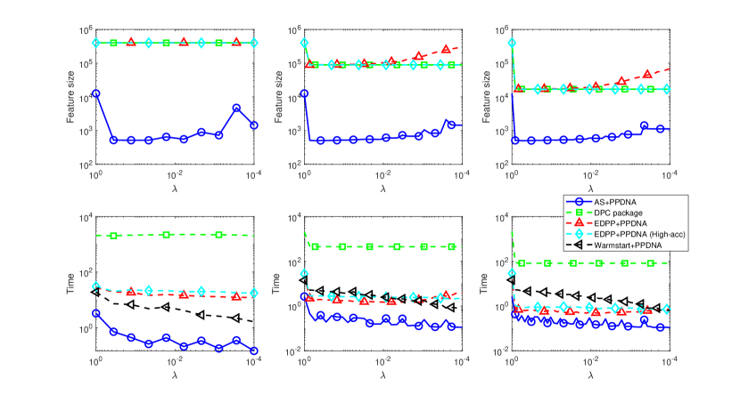
Fig. 1: Comparison among different combinations of screening strategies and algorithms for generating solution paths for the Lasso model of size $(m,g,p)=(500,20,20000)$ with $\lambda$ from $1$ to $10^{-4}$. Left: $10$ equally divided grid points on the $\log_{10}$ scale; Middle: $30$ equally divided grid points on the $\log_{10}$ scale; $50$ equally divided grid points on the $\log_{10}$ scale.

Specifically, we compare AS+SSNAL with the following algorithms.

• The algorithm implemented in the DPC Package. Note that the screening rule implemented in the DPC Package is the Enhanced Dual Projection onto Polytope (EDPP), which is a state-of-the-art safe elimination method for Lasso problems. In order to solve the reduced Lasso problems, the DPC package employs the function “LeastR” in the solver SLEP [19].

• Here we combine the safe elimination method EDPP with the SSNAL to fairly compare the AS and the EDPP. We consider two scenarios where the SSNAL solves the reduced problems to a median accuracy ($\epsilon=10^{-6}$) and a high accuracy ($\epsilon=10^{-10}$). The reason why we run the experiments for both median accuracy and high accuracy is that, the safe elimination method EDPP is based on the assumption that the reduced problems are solved exactly.

• Warmstart+SSNAL. For comparison, we also generate the solution paths with the warm-start technique.

In Figure 1, the upper row shows the (averaged) feature size for each $\lambda$ during the path generation and the lower row shows the running time required for each algorithm. We can see from the aspect of performance of dimension reduction that the AS performs much better than the EDPP by a large margin. It should be mentioned that, the AS is an aggressive dimension reduction strategy which needs several rounds of sieving to solve the problem with a given $\lambda$, while the EDPP is a safe elimination method which only needs to solve one larger reduced problem for each $\lambda$. For example, when we choose $30$ grid points of $\lambda$ for generating solution paths of Lasso problems, for each $\lambda$ except the first one, the EDPP results in a reduced problem with the feature size of around $10^{5}$, while the AS needs to solve two or three reduced problems with the feature sizes of around $10^{3}$. Another important observation is that, the AS gives good performance in dimension reduction for the sequence of $\lambda$ with various different gaps, while the EDPP only works well for that with smaller gaps. From the aspect of running time, we can see that AS+SSNAL outperforms other algorithms by a large margin, while the algorithm implemented in the DPC package gives the worst performance. The reason is that the “aggressive” AS enables us to obtain reduced problems with much smaller sizes than the “safe” EDPP, and the SSNAL is the state-of-the-art method for solving Lasso problems, especially for high-dimensional cases. We note that EDPP+SSNAL also gives better performance than the algorithm implemented in the DPC package, which again demonstrates the advantage of the SSNAL, as all of them use the EDPP and need to solve the reduced problems with similar sizes for each $\lambda$.

5.4.2 Comparison on the group lasso linear regression problems

Now, we are going to generate solution paths for the group lasso models.

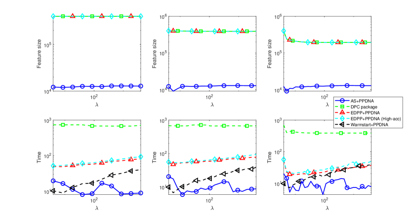
Fig. 2: Comparison among different combinations of screening strategies and algorithms for generating solution paths for the group lasso model of size $(m,g,p)=(400,10000,40)$ with $w$ being the vector of all ones, $\lambda_{1}=0$, and $\lambda_{2}$ from $2500$ to $2.5$. Left: $10$ equally divided grid points on the $\log_{10}$ scale; Middle: $20$ equally divided grid points on the $\log_{10}$ scale; $30$ equally divided grid points on the $\log_{10}$ scale.

The comparison among different combinations of screening strategies and algorithms for generating solution paths for the group lasso model is shown in Figure 2. Note that in the algorithm implemented in the DPC package, the reduced group lasso problems are solved by the function “glLeastR” in the solver SLEP. We can see from the figure that AS+SSNAL gives the best performance for all instances and the algorithm implemented in the DPC package gives the worst. EDPP+SSNAL also gives satisfactory results due to the superior performance of SSNAL for solving group lasso problems.

6 Conclusion

In this paper, we design an adaptive sieving strategy for solving general sparse optimization models and further generating solution paths for a given sequence of parameters. For each reduced problem involved in the AS strategy, we allow it to be solved inexactly. The finite termination property of the AS strategy has also been established. Extensive numerical experiments have been conducted to demonstrate the effectiveness and flexibility of the AS strategy to solve large-scale machine learning models.

References

- [1] A. Beck and M. Teboulle, A fast iterative shrinkage-thresholding algorithm for linear inverse problems, SIAM Journal on Imaging Sciences, 2 (2009), pp. 183–202.
- [2] R. Bellman, Adaptive control processes: A guided tour, 1961.
- [3] M. Bogdan, E. Van Den Berg, C. Sabatti, W. Su, and E. J. Candès, SLOPE—adaptive variable selection via convex optimization, The Annals of Applied Statistics, 9 (2015), p. 1103.
- [4] F. Campbell and G. I. Allen, Within group variable selection through the exclusive lasso, Electronic Journal of Statistics, 11 (2017), pp. 4220–4257.
- [5] C.-C. Chang and C.-J. Lin, LIBSVM: A library for support vector machines, ACM Transactions on Intelligent Systems and Technology, 2 (2011), pp. 1–27.
- [6] M. Du, An Inexact Alternating Direction Method of Multipliers for Convex Composite Conic Programming with Nonlinear Constraints, PhD thesis, Department of Mathematics, National University of Singapore, Singapore, 2015.
- [7] J. Eckstein and D. P. Bertsekas, On the Douglas-Rachford splitting method and the proximal point algorithm for maximal monotone operators, Mathematical Programming, 55 (1992), pp. 293–318.
- [8] Y. C. Eldar and M. Mishali, Robust recovery of signals from a structured union of subspaces, IEEE Transactions on Information Theory, 55 (2009), pp. 5302–5316.
- [9] J. Fan and J. Lv, Sure independence screening for ultrahigh dimensional feature space, Journal of the Royal Statistical Society: Series B (Statistical Methodology), 70 (2008), pp. 849–911.
- [10] L. E. Ghaoui, V. Viallon, and T. Rabbani, Safe feature elimination for the lasso and sparse supervised learning problems, Pacific Journal of Optimization, 8 (2012), pp. 667–698.
- [11] R. Glowinski and A. Marroco, Sur l’approximation, par éléments finis d’ordre un, et la résolution, par pénalisation-dualité d’une classe de problèmes de dirichlet non linéaires, Revue française d’automatique, informatique, recherche opérationnelle. Analyse numérique, 9 (1975), pp. 41–76.
- [12] L. Grippo and M. Sciandrone, On the convergence of the block nonlinear Gauss–Seidel method under convex constraints, Operations Research Letters, 26 (2000), pp. 127–136.
- [13] L. Jacob, G. Obozinski, and J.-P. Vert, Group lasso with overlap and graph lasso, in Proceedings of the 26th Annual International Conference on Machine Learning, 2009, pp. 433–440.
- [14] E. Kalnay, M. Kanamitsu, R. Kistler, W. Collins, D. Deaven, L. Gandin, M. Iredell, S. Saha, G. White, J. Woollen, Y. Zhu, M. Chelliah, W. Ebisuzaki, W. Higgins, J. Janowiak, K. C. Mo, C. Ropelewski, J. Wang, A. Leetmaa, R. Reynolds, R. Jenne, and D. Joseph, The NCEP/NCAR 40-year reanalysis project, Bulletin of the American Meteorological Society, 77 (1996), pp. 437–472.
- [15] M. Kowalski, Sparse regression using mixed norms, Applied and Computational Harmonic Analysis, 27 (2009), pp. 303–324.
- [16] J. Larsson, M. Bogdan, and J. Wallin, The strong screening rule for slope, in Proceedings of the 34th International Conference on Neural Information Processing Systems, NIPS’20, 2020.
- [17] X. Li, D. F. Sun, and K.-C. Toh, A highly efficient semismooth Newton augmented Lagrangian method for solving Lasso problems, SIAM Journal on Optimization, 28 (2018), pp. 433–458.
- [18] M. Lin, Y. Yuan, D. F. Sun, and K.-C. Toh, A highly efficient algorithm for solving exclusive lasso problems, arXiv preprint arXiv:2306.14196, (2023).
- [19] J. Liu, S. Ji, and J. Ye, SLEP: Sparse learning with efficient projections, Arizona State University, 6 (2009), p. 7.
- [20] Z. Luo, D. F. Sun, K.-C. Toh, and N. Xiu, Solving the OSCAR and SLOPE models using a semismooth Newton-based augmented Lagrangian method., Journal of Machine Learning Research, 20 (2019), pp. 1–25.
- [21] R. T. Rockafellar, Convex Analysis, Princeton University Press, 1970.
- [22] R. T. Rockafellar, Monotone operators and the proximal point algorithm, SIAM Journal on Control and Optimization, 14 (1976), pp. 877–898.
- [23] S. Sardy, A. G. Bruce, and P. Tseng, Block coordinate relaxation methods for nonparametric wavelet denoising, Journal of Computational and Graphical Statistics, 9 (2000), pp. 361–379.
- [24] R. Tibshirani, Regression shrinkage and selection via the lasso, Journal of the Royal Statistical Society: Series B (Methodological), 58 (1996), pp. 267–288.
- [25] R. Tibshirani, J. Bien, J. Friedman, T. Hastie, N. Simon, J. Taylor, and R. J. Tibshirani, Strong rules for discarding predictors in lasso-type problems, Journal of the Royal Statistical Society: Series B (Statistical Methodology), 74 (2012), pp. 245–266.
- [26] P. Tseng, Dual coordinate ascent methods for non-strictly convex minimization, Mathematical Programming, 59 (1993), pp. 231–247.
- [27] J. Wang, P. Wonka, and J. Ye, Lasso screening rules via dual polytope projection, Journal of Machine Learning Research, 16 (2015), pp. 1063–1101.
- [28] J. Wang, J. Zhou, P. Wonka, and J. Ye, Lasso screening rules via dual polytope projection, in Advances in Neural Information Processing Systems, 2013, pp. 1070–1078.
- [29] Z. J. Xiang, Y. Wang, and P. J. Ramadge, Screening tests for lasso problems, IEEE Transactions on Pattern Analysis and Machine Intelligence, 39 (2016), pp. 1008–1027.
- [30] M. Yuan and Y. Lin, Model selection and estimation in regression with grouped variables, Journal of the Royal Statistical Society: Series B (Statistical Methodology), 68 (2006), pp. 49–67.
- [31] Y. Zeng and P. Breheny, The biglasso package: A memory- and computation-efficient solver for Lasso model fitting with big data in R, The R Journal, 12 (2021), pp. 6–19.
- [32] Y. Zeng, T. Yang, and P. Breheny, Hybrid safe–strong rules for efficient optimization in lasso-type problems, Computational Statistics & Data Analysis, 153 (2021), p. 107063.
- [33] Y. Zhang, N. Zhang, D. F. Sun, and K.-C. Toh, An efficient Hessian based algorithm for solving large-scale sparse group Lasso problems, Mathematical Programming, (2020), pp. 1–41.
- [34] Y. Zhou, R. Jin, and S. C.-H. Hoi, Exclusive lasso for multi-task feature selection, in Proceedings of the Thirteenth International Conference on Artificial Intelligence and Statistics, 2010, pp. 988–995.
- [35] Z. Zhou and A. M.-C. So, A unified approach to error bounds for structured convex optimization problems, Mathematical Programming, 165 (2017), pp. 689–728.
- [36] H. Zou and T. Hastie, Regularization and variable selection via the elastic net, Journal of the Royal Statistical Society: Series B (Statistical Methodology), 67 (2005), pp. 301–320.