Quantum optimization algorithm based on multistep quantum computation

Abstract

We present a quantum algorithm for finding the minimum of a function based on multistep quantum computation and apply it for optimization problems with continuous variables, in which the variables of the problem are discretized to form the state space of the problem. Usually the cost for solving the problem increases dramatically with the size of the problem. In this algorithm, the dimension of the search space of the problem can be reduced exponentially step by step. We construct a sequence of Hamiltonians such that the search space of a Hamiltonian is nested in that of the previous one. By applying a multistep quantum computation process, the optimal vector is finally located in a small state space and can be determined efficiently. One of the most difficult problems in optimization is that a trial vector is trapped in a deep local minimum while the global minimum is missed, this problem can be alleviated in our algorithm and the runtime is proportional to the number of the steps of the algorithm, provided certain conditions are satisfied. We have tested the algorithm for some continuous test functions.

I Introduction

Optimization problem is one of the most important problems in science and engineering. It includes a wide class of problems ranging from molecular modeling, quantum mechanical calculations, machine learning, to combinatorial optimization. These problems can be classified into different categories, e.g., continuous or discrete optimization, constrained or unconstrained optimization, convex or nonconvex optimization, differentiable or nondifferentiable optimization, deterministic or stochastic optimization weise ; boyd ; noce ; flet ; flou , etc. There is no universal optimization algorithm. Most classical optimization algorithms start with a trial vector that is varied by using different techniques to find the optimum of an objective function. The cost of the algorithms can become very expensive due to the increase of the dimension of the state space of the problem, which is known as “the curse of dimension”. Another problem that often happens for optimization algorithms is that the trial vector is trapped in a deep local minimum, while missing the global minimum of the objective function.

Optimization has also been studied in the framework of quantum computation. Adiabatic quantum computing (AQC) is designed for solving combinatorial optimization problems farhi , in which starting with the ground state of a simple initial Hamiltonian, the system is evolved adiabatically to a final Hamiltonian whose ground state encodes the solution to the optimization problem. Despite the theoretical guarantee of the adiabatic theorem, the condition of adiabaticity in AQC is difficult to maintain in practice, since the allowed rate of evolution is determined by the minimum energy gap between the ground and the first excited states of the adiabatic evolution Hamiltonian, which is not known a priori. Quantum annealing is a heuristic quantum optimization algorithm fin ; kad ; bro ; san ; joh that can be viewed as a relaxation of AQC, where the conditions of adiabaticity are not met and the evolution time from an initial Hamiltonian to the final Hamiltonian is determined heuristically. Whether or not quantum annealing can provide quantum speed-up over classical heuristic algorithms is still not clear. Variational quantum algorithms such as quantum approximate optimization algorithm (QAOA) qaoa are hybrid quantum-classical algorithms designed for near-term noisy intermediate-scale quantum computers nisq without performance guarantees. It is known that in the infinite depth limit, the QAOA recovers adiabatic evolution and would converge to the optimal solution. The gradient decent methods are used for optimization problems with continuous variables. The methods find local minima of a smooth function by moving along the direction of the steepest descent. Quantum algorithm provides an efficient way in calculating numerical gradients jor , and has been used in iterative algorithms for polynomial optimization reb . Optimization algorithms based on gradient decent require that the objective function to be smooth, and they have the problem of being trapped in a local minimum and missing the global minimum. Besides, as the dimensionality of the problem increases, the search of the phase space becomes more and more complicated, and the complexity of the algorithm increases. Another approach for continuous optimization is by using Grover’s search algorithm grover . Continuous optimization problems can be discretized and mapped to a search problem, thereby solved by using Grover’s algorithm. The Grover adaptive search algorithms iteratively apply Grover search to find the optimum value of an objective function durr ; pro ; bul ; bari ; kowa ; liu ; gill , and can achieve quadratic speedup over classical search algorithms. However, these brute force methods are prohibitively expensive due to the large search space of the problems.

In a recent work wyx , we proposed an efficient quantum algorithm for solving a search problem with nested structure through multistep quantum computation. The problem can be decomposed and the search space of the problem can be reduced in a polynomial rate. The runtime of the algorithm is proportional to the number of steps of the algorithm. In this work, we generalize this algorithm for optimization problems with continuous variables.

The nested structured search problem wyx is a search problem that contains $N$ items with one target item, and can be decomposed by using $m$ [$O(\log N)$] oracles to construct $m$ Hamiltonians, respectively, as

$$H_{P_{i}}=-\sum_{\eta_{i}\in\Pi_{i}}|\eta_{i}\rangle\langle\eta_{i}|,\text{ \ \ }i=1,\ldots,m$$ (1)

and

$$H_{P_{m}}=H_{m}=H_{P}=-|\eta\rangle\langle\eta|,$$ (2)

where the set $\Pi_{i}$ contains $N_{i}$ marked items in the $N$ items and $|\eta_{i}\rangle$ are the marked states associated with the marked items, and $|\eta\rangle$ is the target state that defines the problem Hamiltonian of the search problem. These sets are nested as $\Pi_{1}\supset\cdots\supset\Pi_{m-1}\supset\Pi_{m}$ with sizes $N_{1}$, $\cdots$, $N_{m-1}$, $N_{m}=1$, respectively. The ratio $N_{i-1}/N_{i}$ are polynomial large, and $N_{0}=N$. The goal is to find the the target state $|\eta\rangle$ that is associated with the target item in the set $\Pi_{m}$.

Our algorithm solves the nested structured search problem by finding the ground state of the problem Hamiltonian $H_{P}$ via a multistep quantum computation process, which is realized through quantum resonant transition (QRT) whf0 ; whf2 . In this algorithm, a probe qubit is coupled to an $n$-qubit register $R$ that represents the problem. We construct a sequence of intermediate Hamiltonians to form a Hamiltonian evolution path to the problem Hamiltonian as

$$H_{i}=\frac{N_{i}}{N}H_{0}+\left(1-\frac{N_{i}}{N}\right)H_{P_{i}},\text{ \ \ }i=0,1,\ldots,m-1,$$ (3)

where $H_{0}=-|\psi_{0}\rangle\langle\psi_{0}|$ and $|\psi_{0}\rangle=\frac{1}{\sqrt{N}}\sum_{j=0}^{N-1}|j\rangle$. Then we start from the ground state of the initial Hamiltonian, and evolve it through the ground states of the intermediate Hamiltonians sequentially through QRT to reach the ground state of the problem Hamiltonian. The ground state of an intermediate Hamiltonian is protected in an entangled state of the probe qubit and the register $R$, such that it can be used repeatedly without making copies. Therefore the algorithm circumvents the restriction of the no-cloning theorem noclone1 ; noclone2 and realizes the multistep quantum computation. The algorithm can be run efficiently provided that: ($i$) the energy gap between the ground and the first excited states of each Hamiltonian $H_{i}$ and, ($ii$) the overlaps between ground states of any two adjacent Hamiltonians are not exponentially small. For the nested structured search problem, the conditions of the algorithm are satisfied since the ratio $N_{i-1}/N_{i}$ are polynomial large, therefore it can be solved efficiently, and the conditions for efficiently running our algorithm are not equivalent to those of the AQC algorithms wyx .

In this algorithm, by using the Hamiltonians $H_{P_{i}}$ sequentially in each step, the dimension of the search space of the problem is reduced in a polynomial rate, the solution state to the problem Hamiltonian is obtained step by step. The idea of reducing the search space in a polynomial rate step by step in our algorithm has a classical analogue as follows: suppose there are $80$ balls, all of them have equal weights except one that is lighter than the others. How to find the lighter ball? If we randomly pick up a ball and compare its weight with the other balls, this will take about $40$ trials on average. If we have a balance, then how many times do we have to use the balance to find the lighter ball? According to information theory, the number of times the balance has to be used is $\log 80/\log 3\approx 4$. The procedure is as follows: we divide all the $80$ balls into $3$ groups, each group has $27$, $27$ and $26$ balls, respectively; then pick up the two groups that both have $27$ balls, and use the balance to determine if they have equal weights. If the answer is positive, pick the group with $26$ balls and divide it into $3$ groups again: $9,9,8$; otherwise, take the group that is lighter and divide it into three new groups: $9,9,9$. This process can be repeated until the lighter ball is found. In this example, we can see that the problem is divided into a series of nested sub-problems and the size of the search space is reduced in a rate about $1/3$ by using a balance. The target ball is found through an iterative procedure and the cost is reduced exponentially. By using a different oracle in each step, the QRT procedure in our algorithm emulates the usage of the balance in solving the nested structured search problem.

The procedure for solving the nested structured search problem can be applied for optimization problems that are transformed to finding the ground state of a problem Hamiltonian in quantum computation. Here, we propose a quantum algorithm based on multistep quantum computation for optimization problems with continuous variables. We first discretize the variables of the objective function to construct the state space of the problem. Then we construct a sequence of intermediate Hamiltonians to reach the problem Hamiltonian by decomposing the problem using a set of threshold values, and apply a multistep quantum computation process to reduce the search space of the problem step by step. The solution vector to the optimization problem is narrowed in a small state space and can be determined efficiently through measurements. If the search spaces of the Hamiltonians are reduced in a polynomial rate by using an appropriate set of threshold values, then the optimum of the function can be obtained efficiently. Meanwhile if the global minimum of the optimization problem is in the state space of the problem, then it can be obtained efficiently. The problem in many optimization algorithms where the trial vector is trapped in a deep local minimum and missing the global minimum can be avoided in our algorithm, provided the above conditions are satisfied. In quantum computing, the dimension of the Hilbert space of the qubits increases exponentially with the number of qubits, it is more efficient to represent a large state space on a quantum computer than on a classical computer, therefore increasing the probability of finding the global minimum of the problem.

This paper is organized as follows: in Sec. II, we describe the quantum algorithm for optimization problems with continuous variables based on multistep quantum computation; in Sec. III, we apply the algorithm for some test optimization problems, and we close with a discussion.

II Quantum optimization algorithm based on multistep quantum computation

Let $S$ be the domain of $\mathbf{x}$, an optimization problem can be formulated as a minimization problem:

$$\text{minimize }F(\mathbf{x})\text{: subject to }\mathbf{x}\in S,$$ (4)

where $F$ is a real-valued objective function and $\mathbf{x}$ is the vector of the variables. Here we focus on optimization problems with continuous variables, which can be described as follows: for a real-valued function of $r$ variables, $F\left(x_{1},x_{2},\cdots,x_{r}\right)$, find a vector of the variables such that the function has the minimum value. In the following, we present a quantum optimization algorithm based on multistep quantum computation for this problem.

We discretize the continuous variables in the function domain into intervals of same length for all the variables, and map the problem on a quantum computer. For simplicity, suppose each variable is discretized into $l$ elements in its definition domain, the dimension of the state space of the function is $l^{r}$. We prepare $r$ quantum registers and each register contains $\lceil\log_{2}l\rceil$ qubits that represents the elements of the variable. Therefore $n=r\lceil\log_{2}l\rceil$ qubits form the register $R$ that represents the problem with state space of size $N=2^{n}$ on a quantum computer. A vector of the discretized variables $x_{1}^{(i)}$, $x_{2}^{(j)}$, $\ldots$, $x_{r}^{(k)}$ is represented by state $|ij\cdots k\rangle$, where $x_{s}^{(j)}$ represents the $j$th element of the variable $x_{s}$. The states $|i\rangle$, $|j\rangle$, $\cdots$, $|k\rangle$ are binary representation of the elements $x_{1}^{(i)}$, $x_{2}^{(j)}$, $\ldots$, $x_{r}^{(k)}$ on the quantum registers. These vectors form the computational basis states (CBS) of $r$ quantum registers of dimension $N$ as $|J\rangle=|i\rangle|j\rangle\ldots|k\rangle$, $J=0$, $1$, $\ldots$, $N-1$, and the corresponding function value is $F\left(x_{1}^{(i)},x_{2}^{(j)},\ldots,x_{r}^{(k)}\right)=F\left(J\right)=F_{J}$. The task is to find the vector $|Q\rangle=|q_{1}\rangle|q_{2}\rangle\ldots|q_{r}\rangle$ such that $F\left(x_{1}^{(q_{1})},x_{2}^{(q_{2})},\ldots,x_{r}^{(q_{r})}\right)$ is the minimum of the function $F$.

By using an oracle $O_{F}$ where $O_{F}|J\rangle|0\rangle=|J\rangle|F\left(J\right)\rangle$, the Hamiltonian of the optimization problem can be constructed as

$$H_{F}|J\rangle=F_{J}|J\rangle,$$ (5)

where $F_{J}$ are eigenvalues of $H_{F}$ with corresponding eigenstates $|J\rangle$. The problem of finding the minimum of the function $F$ is transformed to finding the ground state of the Hamiltonian $H_{F}$ and its corresponding eigenvalue. We apply a multistep quantum computation process for solving this problem. We first estimate the range of the function value as $\left[F_{\min}\text{, }F_{\max}\right]$, and prepare a set of threshold values {$d_{1}$, $d_{2}$, $\ldots$, $d_{m}$}, and $F_{\max}>d_{1}>d_{2}>\ldots>d_{m}>F_{\min}$. Then we construct $m$ Hamiltonians as:

$$H_{P_{i}}|J\rangle=h_{J}|J\rangle,\text{ \ \ }i=1,\ldots,m$$ (6)

where

$$h_{J}=\Bigg{\{}\begin{array}[]{c}\!\!-1,\,\mathrm{if}\,F_{J}\leq d_{i},\\ \!\!\hskip 0.02205pt0,\,\mathrm{if}\,F_{J}>d_{i}\,,\end{array}$$ (7)

and $H_{P_{m}}=H_{m}=H_{P}$. This can be achieved by using an oracle that recognizes whether $F_{J}$ is larger or less than a threshold value $d_{i}$. It is a comparison logic circuitry and can be implemented efficiently on a quantum computer (nc, , p.264) durr ; bari ; grandunif . The CBS associated with integers that are less than or equal to $d_{i}$ form a set $A_{i}$ with size $N_{i}$. They have the nested structure as $A_{m}\subset A_{m-1}\subset\cdots\subset A_{1}$. The ground state of the problem Hamiltonian $H_{P}$ contains CBS in $A_{m}$ with eigenvalues that are below the threshold value $d_{m}$. We construct a sequence of Hamiltonians that form a Hamiltonian evolution path to the problem Hamiltonian $H_{P}$ as

$$H_{i}=\frac{M_{i}}{N}H_{0}+\left(1-\frac{M_{i}}{N}\right)H_{P_{i}},\text{ \ \ }i=0,1,\ldots,m-1,$$ (8)

where $H_{0}=-|\psi_{0}\rangle\langle\psi_{0}|$ and $|\psi_{0}\rangle=\frac{1}{\sqrt{N}}\sum_{j=0}^{N-1}|j\rangle$, and $M_{i}$ is an approximate estimation of $N_{i}$. We have demonstrated that as $M_{i}=N_{i}$, the conditions for efficiently running the algorithm are satisfied provided that the ratio $N_{i-1}/N_{i}$ are polynomial large wyx . The parameters $M_{i}$ can be estimated efficiently by using the Monte Carlo sampling method wanglandau , and we can adjust the threshold values such that the ratio $N_{i-1}/N_{i}$ are polynomial large. Detailed analysis of the effect of $M_{i}$ on the efficiency of the algorithm is presented in the appendix. The ground state of $H_{P}$ can be obtained through the following multistep quantum computation process based on QRT in $m$ steps. We use the $i$th step of the algorithm to illustrate the procedures.

In the $i$th step, given the Hamiltonian $H_{i-1}$, its ground state eigenvalue $E_{0}^{\left(i-1\right)}$ and the ground state $|\varphi_{0}^{\left(i-1\right)}\rangle$ obtained from the previous step, we are to prepare the ground state $|\varphi_{0}^{\left(i\right)}\rangle$ of $H_{i}$ by using the QRT method. The algorithm requires ($n+1$) qubits with a probe qubit coupling to the $n$-qubit register $R$. The algorithm Hamiltonian of the $i$th step is constructed as

$$H^{\left(i\right)}=-\frac{1}{2}\omega\sigma_{z}\otimes I_{N}+H_{R}^{\left(i\right)}+c\sigma_{x}\otimes I_{N},$$ (9)

where

$$H_{R}^{\left(i\right)}=\alpha_{i}|1\rangle\langle 1|\otimes H_{i-1}+|0\rangle\langle 0|\otimes H_{i}\mathbf{,}\text{\ }i=1,2,\cdots,m,$$ (10)

$I_{N}$ is the $N$-dimensional identity operator, and $\sigma_{x}$ and $\sigma_{z}$ are the Pauli matrices. The first term in Eq. ($9$) is the Hamiltonian of the probe qubit, the second term contains the Hamiltonian of the register $R$ and describes the interaction between the probe qubit and $R$, and the third term is a perturbation with $c\ll 1$. The parameter $\alpha_{i}$ is used to re-scale the energy levels of $H_{i-1}$, and the ground state energy of $\alpha_{i}H_{i-1}$ is used as a reference energy level to the ground state eigenvalue $E_{0}^{\left(i\right)}$ of $H_{i}$. The initial state of the $(n+1)$ qubits is set as $|1\rangle|\varphi_{0}^{\left(i-1\right)}\rangle$, which is an eigenstate of $H_{R}^{\left(i\right)}$ with eigenvalue $\alpha_{i}E_{0}^{\left(i-1\right)}$. First we obtain the eigenvalue $E_{0}^{\left(i\right)}$ of $H_{i}$ by using the QRT method through varying the frequency of the probe qubit as shown in Ref. wyx . Then we set $\alpha_{i}=\left(E_{0}^{\left(i\right)}-\omega\right)/E_{0}^{\left(i-1\right)}$, such that the condition of $E_{0}^{\left(i\right)}-\alpha_{i}E_{0}^{\left(i-1\right)}=\omega$ for resonant transition between the probe qubit and the transition between states $|\varphi_{0}^{\left(i-1\right)}\rangle$ and $|\varphi_{0}^{\left(i\right)}\rangle$ is satisfied. When obtaining the eigenvalue $E_{0}^{\left(i\right)}$ of $H_{i}$, we can also obtain the overlap $g_{0}^{(i)}=\langle\varphi_{0}^{(i-1)}|\varphi_{0}^{(i)}\rangle$ between the ground states of $H_{i-1}$ and $H_{i}$ through the Rabi’s formula cohen . Then we can set the optimal runtime $t_{i}=\pi/(2cg_{0}^{(i)})$ at which the probability for the system to be evolved to the state $|0\rangle|\varphi_{0}^{\left(i\right)}\rangle$ reaches its maximum. The procedures for obtaining the ground state of $H_{i}$ are summarized as follows:

($i$) Initialize the probe qubit to its excited state $|1\rangle$ and the register $R$ in state $|\varphi_{0}^{\left(i-1\right)}\rangle$;

($ii$) Implement the unitary evolution operator $U(t_{i})=\exp\left(-iH^{\left(i\right)}t_{i}\right)$;

($iii$) Read out the state of the probe qubit.

The system is approximately in state $\sqrt{1-p_{0}^{\left(i\right)}}|1\rangle|\varphi_{0}^{\left(i-1\right)}\rangle+\sqrt{p_{0}^{\left(i\right)}}|0\rangle|\varphi_{0}^{\left(i\right)}\rangle$ as the resonant transition occurs, where $p_{0}^{\left(i\right)}=\sin^{2}\left(ct_{i}g_{0}^{(i)}\right)$ is the decay probability of the probe qubit of the $i$th step. The state $|\varphi_{0}^{\left(i-1\right)}\rangle$ from the previous step is protected in this entangled state. By performing a measurement on the probe qubit, if the probe decays to its ground state $|0\rangle$, it indicates that the resonant transition occurs and the system evolves from the state $|1\rangle|\varphi_{0}^{\left(i-1\right)}\rangle$ to the state $|0\rangle|\varphi_{0}^{\left(i\right)}\rangle$; otherwise if the probe qubit stays in state $|1\rangle$, it means that the register $R$ remains in state $|\varphi_{0}^{\left(i-1\right)}\rangle$, then we repeat procedures $ii$)-$iii$) until the probe qubit decays to its ground state $|0\rangle$. Therefore we can obtain the ground state $|\varphi_{0}^{\left(i\right)}\rangle$ of $H_{i}$ deterministically. By protecting the state $|\varphi_{0}^{\left(i-1\right)}\rangle$ through entanglement, the state can be used repeatedly without copying it, such that the algorithm realizes multistep quantum computation. The runtime of the algorithm is proportional to the number of steps of the algorithm, and the success probability of the algorithm is polynomial large by setting the coupling coefficient $c$ appropriately wyx . After running the algorithm for $m$ steps, we obtain the ground state of the problem Hamiltonian $H_{P}$, which is a superposition state of a few CBS with eigenvalues below the threshold value $d_{m}$. Then we can perform measurement on the state and find the CBS that has the minimum function value, therefore solving the optimization problem. We can run the algorithm for a few rounds by discretizing the variables in the neighborhood of the optimized vector to improve the precision of the solution to the optimization problem.

The algorithm can be run efficiently if both the energy gap between the ground and the first excited states of each Hamiltonian $H_{i}$ and the overlap between ground states of any two adjacent Hamiltonians $g_{0}^{(i)}$ are not exponentially small. By solving the eigen-problem of the Hamiltonian $H_{i}$, these conditions can be satisfied if the ratio $N_{i-1}/N_{i}$ are polynomial large, and the parameters $M_{i}$ are set such that: the point $\left(N_{i}/N,M_{i}/N\right)$ is far away from the neighborhood of the point $\left(0,1/2\right)$, and $2M_{i}\left(N-N_{i}\right)<N^{2}$. Detailed analysis is shown in the appendix.

III Application of the algorithm for some test functions

We now apply the quantum optimization algorithm described above for some test functions of optimization problem: the Damavandi function, the Griewank function and the Price function.

III.1 The Damavandi function

The two dimensional Damavandi function is defined as

$$f_{\text{Damavandi}}\left(x_{1},x_{2}\right)=\left[1-\left|\frac{\sin\left[\pi\left(x_{1}-2\right)\right]\sin\left[\pi\left(x_{2}-2\right)\right]}{\pi^{2}\left(x_{1}-2\right)\left(x_{2}-2\right)}\right|^{5}\right]\left[2+\left(x_{1}-7\right)^{2}+2\left(x_{2}-7\right)^{2}\right],$$ (11)

and the graph of this function is shown in Fig. $1$. It has a very sharp global minimum of zero at {$x_{1}=2$, $x_{2}=2$}. For classical optimization algorithms based on the gradients methods, it is very easy for a trial vector to be trapped in the bowl-like local minimum, while missing the global minimum. The overall success probability of current global optimization algorithms for finding the global minimum of this function is about $0.25\%$ testfunc .

To apply our algorithm for this optimization problem, the two variables of the Damavandi function are discretized into $281$ elements evenly with an interval of $0.05$ in the range $\left[0,14\right]$. The dimension of the state space of the function is $78961$. By discretizing the value of the function in an interval of $0.01$ in the range of $\left[0,149\right]$, and counting the number of states in each interval, we can obtain the distribution of states of the function in each energy interval as shown in Fig. $2$. The largest degeneracy is about $56$, which is a small number compare to the dimension of the state space. We construct a set of threshold values as {$d_{1}=70$, $d_{2}=30$, $d_{3}=15$, $d_{4}=7$, $d_{5}=4$, $d_{6}=3$, $d_{7}=2.5$, $d_{8}=2.2$, $d_{9}=2.1$, $d_{10}=2.02$, $d_{11}=2.0$, $d_{12}=1.0$}, and run the algorithm. The dimension of the corresponding state space in each step of the algorithm are reduced to {$56634$, $24939$, $11573$, $4452$, $1772$, $892$, $448$, $178$, $94$, $20$, $5$, $1$}, respectively. The dimension of the state space is reduced smoothly with reduction rates of {$0.717$, $0.440$, $0.464$, $0.385$, $0.398$, $0.503$, $0.502$, $0.397$, $0.528$, $0.213$, $0.250$, $0.200$} in each step of the algorithm, respectively. The parameter $M_{i}$ can be estimated through Monte Carlo sampling, if it is set approximately as $N_{i}$ above, the conditions of the algorithm can be satisfied. The ratio $M_{i}/N$ that are closest to $1/2$ is $0.316$.

We can see that the dimension of the state space is reduced to a few CBS after a number of steps. Therefore the final state that encodes the solution to the optimization problem can be readout and checked efficiently to find the global optimum of the function.

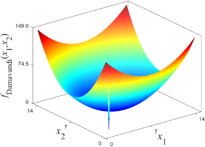
Figure 1: (Color online) The graph of the Damavandi function.

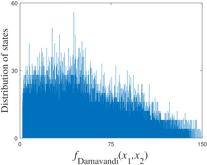
Figure 2: Distribution of states by discretizing the value of the Damavandi function in intervals of $0.01$.

III.2 The Griewank function

The Griewank function has the form

$$f_{\text{Griewank}}\!\left(\!x_{1},\cdots,x_{n}\!\right)\!=\!\frac{1}{4000}\sum_{k=1}^{n}\!x_{k}^{2}\!-\!\prod_{k=1}^{n}\!\cos\!\left(\!\frac{x_{k}}{\sqrt{k}}\!\right)\!+\!1.$$ (12)

Fig. $3$ shows the second-order Griewank function with two variables, we can see that the function has many local minima. For classical optimization algorithms, it is very easy for a trial vector to be trapped in one of the local minima, while missing the global minimum of the function. This situation can be avoided in our algorithm.

We discretize the two variables of the Griewank function into $801$ elements evenly with interval of $0.1$ in the range $\left[-40,40\right]$. The dimension of the state space of the function is $641601$. By discretizing the function value in intervals of $0.0001$, the distribution of states in each energy interval of the function is shown in Fig. $4$. The largest degeneracy is $32$. The threshold value set is constructed as {$d_{1}=1.0$, $d_{2}=0.6$, $d_{3}=0.4$, $d_{4}=0.3$, $d_{5}=0.2$, $d_{6}=0.1$, $d_{7}=0.06$, $d_{8}=0.04$, $d_{9}=0.02$, $d_{10}=0.01$, $d_{11}=0.005$, $d_{12}=0.002$}. The sizes of the corresponding state spaces for each step of the algorithm are {$197363$, $76951$, $34453$, $18937$, $8283$, $2033$, $723$, $319$, $77$, $23$, $5$, $1$}, respectively. The dimension of the state space of the problem is reduced smoothly in each step of the algorithm in rate of {$0.31$, $0.39$, $0.45$, $0.55$, $0.44$, $0.25$, $0.36$, $0.44$, $0.24$, $0.30$, $0.22$, $0.20$}, respectively. After running the algorithm for a number of steps, the state space of the problem is reduced to a very small space and can be readout to calculate the corresponding function value and find the global minimum.

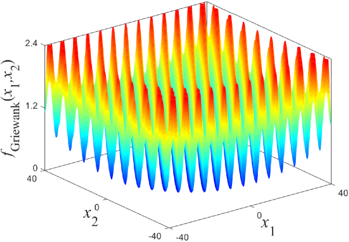
Figure 3: (Color online) The second-order Griewank function.

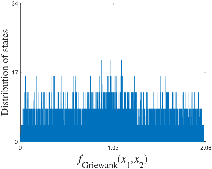
Figure 4: Distribution of states by discretizing the value of the second-order Griewank function in intervals of $0.0001$.

III.3 The Price function

The Price$01$ function can be written in form of

$$f_{\text{Price}}\left(x_{1},x_{2}\right)=\left(\left|x_{1}\right|-5\right)^{2}+\left(\left|x_{2}\right|-5\right)^{2},$$ (13)

with four minima as shown in Fig. $5$. Our algorithm can be applied to obtain the four vectors corresponding to the minimum of the function in a degenerate state.

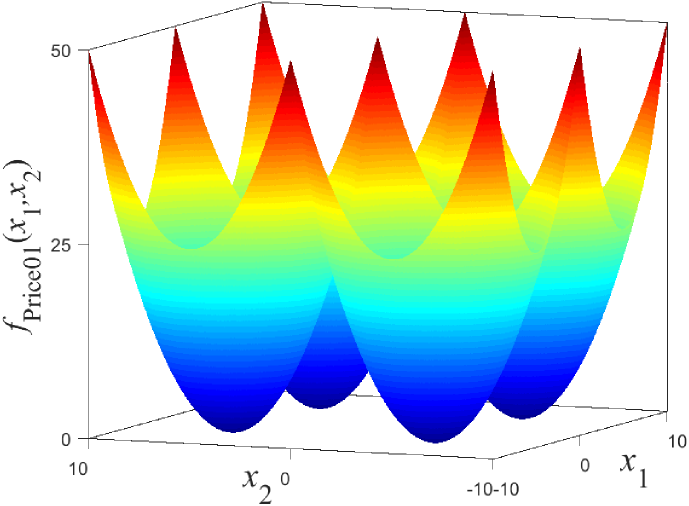
Figure 5: (Color online) The Price$01$ function.

The two variables of the Price function are discretized into $201$ elements evenly with an interval of $0.1$ in the range $\left[-10,10\right]$. The dimension of the state space of the problem is $40401$. A set of threshold values is constructed as {$d_{1}=20$, $d_{2}=10$, $d_{3}=5$, $d_{4}=2$, $d_{5}=1$, $d_{6}=0.5$, $d_{7}=0.2$, $d_{8}=0.1$, $d_{9}=0.05$, $d_{10}=0.02$, $d_{11}=0.01$}. The dimension of the corresponding state space in each round of the algorithm are reduced to {$25108$, $12532$, $6260$, $2484$, $1220$, $596$, $244$, $116$, $52$, $20$, $4$}, respectively. The corresponding reduction rates in each round of the algorithm are {$0.62$, $0.50$, $0.50$, $0.40$, $0.49$, $0.49$, $0.41$, $0.48$, $0.45$, $0.38$, $0.20$}. The final state is in an equal superposition of the four global minima of the function and can be obtained by readout of the state of the circuit.

IV Discussion

In this work, we present a quantum optimization algorithm for solving optimization problems with continuous variables based on multistep quantum computation. The state space of the problem is constructed by discretizing the variables of the objective function. By applying a multistep quantum computation process, the search space of the problem can be reduced step by step. We construct a sequence of Hamiltonians based on a set of threshold values, such that the search spaces corresponding to the Hamiltonians form a nested structure. If the dimension of search spaces is reduced sequentially in polynomial rate, then the algorithm can be run efficiently. The reduction rate can be adjusted by setting the threshold values appropriately. The final state obtained by the algorithm is a superposition of a few CBS (or a CBS) and the minimum of the function can be determined efficiently by measuring the state and evaluating the corresponding function value.

One of the most difficult problems for optimization algorithms is that a trial vector is trapped in a deep local minimum, while missing the global minimum. In our algorithm, we locate the global minimum of the problem by using a number of threshold values, and obtain the corresponding state vector through a multistep quantum computation process by narrowing the search space of the problem step by step. The global minimum can be obtained if it is in the state space of the problem and the conditions of the algorithm are satisfied. One advantage of quantum computing is that exponential number of CBS can be stored in polynomial number of qubits. Therefore we can construct a large state space of the problem by using a small number of qubits, such that increasing the probability of finding the global minimum of the objective function. The precision of the algorithm can be improved by running the algorithm for a few rounds in the neighborhood of the minimum being found.

Appendix A Solving the eigen-problem of the intermediate Hamiltonians

In the following, we solve the eigen-problem of the intermediate Hamiltonian to calculate the energy gap between the ground and the first excited states of the Hamiltonian, and the overlap between the ground states of two adjacent Hamiltonians.

In the quantum optimization algorithm, we construct a sequence of intermediate Hamiltonians to form a Hamiltonian evolution path to the problem Hamiltonian as

$$H_{i}=\frac{M_{i}}{N}H_{0}+\left(1-\frac{M_{i}}{N}\right)H_{P_{i}},\text{ \ }i=1,2,\cdots,m$$ (14)

where

$$H\!_{0}\!\!=-|\psi_{0}\rangle\langle\psi_{0}|,$$ (15)

with $|\psi_{0}\rangle=\frac{1}{\sqrt{N}}\sum_{j=0}^{N-1}|j\rangle$, and

$$H_{P_{i}}=-\sum_{q_{i}\in A_{i}}|q_{i}\rangle\langle q_{i}|,$$ (16)

where $A_{1}\supset\cdots\supset A_{m-1}\supset A_{m}$ are determined by Eqs. ($6$) and ($7$), and the sizes of the sets $A_{1}$, $\cdots$, $A_{m}$ are $N_{1}$, $\cdots$, $N_{m}$, respectively, and $N_{1}>\cdots>N_{m}$. Let $H_{m}=H_{P}=H_{P_{m}}$ and the set $A_{m}$ contains the target states $|q\rangle$ with size $N_{m}$. We construct a Hamiltonian evolution path $H_{0}\rightarrow H_{1}\rightarrow\cdots\rightarrow H_{m}=H_{P}$ and start from the ground state $|\varphi_{0}^{(0)}\rangle$ of $H_{0}$, evolve it through ground states of the intermediate Hamiltonians sequentially via quantum resonant transition (QRT), finally reach the ground state $|\varphi_{0}^{(m)}\rangle$ of $H_{P}$ in $m$ steps. The algorithm can be run efficiently provided: ($i$) the energy gap between the ground and the first excited states of each Hamiltonian and, ($ii$) the overlaps between ground states of any two adjacent Hamiltonians are not exponentially small.

In the following we solve the eigen-problem of the Hamiltonian $H_{i}$. Let

$$|\psi_{0}\rangle=\frac{1}{\sqrt{N}}\sum_{j=0}^{N-1}|j\rangle=\frac{1}{\sqrt{N}}\sum_{q_{i}\in A_{i}}|q_{i}\rangle+\sqrt{\frac{N-N_{i}}{N}}|q_{i}^{\bot}\rangle.$$ (17)

where

$$|q_{i}^{\bot}\rangle=\frac{1}{\sqrt{N-N_{i}}}\sum_{k\notin A_{i}}|k\rangle.$$ (18)

Then in basis $\left(\left\{|q_{i}\rangle\right\}_{q_{i}\in A_{i}}\text{, }|q_{i}^{\bot}\rangle\right)$, we have

$$H\!_{0}\! = -|\psi_{0}\rangle\langle\psi_{0}|$$ (23)

$$= -\left(\!\begin{array}[]{cccc}\frac{1}{N}&\cdots&\frac{1}{N}&\frac{\sqrt{\!N\!-\!N_{i}}}{N}\\ \vdots&\ddots&\vdots&\vdots\\ \frac{1}{N}&\cdots&\frac{1}{N}&\frac{\sqrt{N\!-\!N_{i}}}{N}\\ \frac{\sqrt{\!N\!-\!N_{i}}}{N}&\cdots&\frac{\sqrt{\!N\!-\!N_{i}}}{N}&\frac{\!N\!-\!N_{i}\!}{N}\!\end{array}\!\right),$$

and

$$H_{P_{i}} = -\sum_{q_{i}\in A_{i}}|q_{i}\rangle\langle q_{i}|$$ (28)

$$= -\!\left(\!\begin{array}[]{cccc}1&\cdots&0&0\\ \vdots&\ddots&\vdots&\vdots\\ 0&\cdots&1&0\\ 0&\cdots&0&0\end{array}\!\right).$$

Then

$$H_{i} = \frac{M_{i}}{N}H_{0}+\left(1-\frac{M_{i}}{N}\right)H_{P_{i}}$$ (34)

$$= -\!\!\left(\!\begin{array}[]{ccccc}\frac{M_{i}}{N^{2}}+1-\frac{M_{i}}{N}&\frac{M_{i}}{N^{2}}&\cdots&\frac{M_{i}}{N^{2}}&\frac{M_{i}\sqrt{\!N\!-\!N_{i}}}{N^{2}}\\ \frac{M_{i}}{N^{2}}&\frac{M_{i}}{N^{2}}+1-\frac{M_{i}}{N}&\cdots&\vdots&\vdots\\ \vdots&\vdots&\ddots&&\\ \frac{M_{i}}{N^{2}}&\frac{M_{i}}{N^{2}}&\cdots&\frac{M_{i}}{N^{2}}+1-\frac{M_{i}}{N}&\frac{M_{i}\sqrt{N\!-\!N_{i}}}{N^{2}}\\ \frac{M_{i}\sqrt{\!N\!-\!N_{i}}}{N^{2}}&\frac{M_{i}\sqrt{\!N\!-\!N_{i}}}{N^{2}}&\cdots&\frac{M_{i}\sqrt{\!N\!-\!N_{i}}}{N^{2}}&\frac{M_{i}\left(N\!-\!N_{i}\right)\!\!}{N^{2}}\end{array}\!\right).$$

Let $n=N_{i}+1$,

$$\mathbf{e}=\left(\begin{array}[]{cccc}1&\cdots&1&1\end{array}\right)_{1\times n}^{T},\qquad\mathbf{e}_{n}=\left(\begin{array}[]{cccc}0&\cdots&0&1\end{array}\right)_{1\times n}^{T},$$ (35)

then $H_{0}$ can be rewritten as

$$H_{0} = -\left(\frac{1}{\sqrt{N}}\mathbf{e}+\frac{\sqrt{N-N_{i}}-1}{\sqrt{N}}\mathbf{e}_{n}\right)\left(\frac{1}{\sqrt{N}}\mathbf{e}+\frac{\sqrt{N-N_{i}}-1}{\sqrt{N}}\mathbf{e}_{n}\right)^{T}$$ (36)

$$= -\frac{1}{N}\mathbf{e}\mathbf{e}^{T}-\frac{\sqrt{N-N_{i}}-1}{N}\left(\mathbf{e}\mathbf{e}_{n}^{T}+\mathbf{e}_{n}\mathbf{e}^{T}\right)-\frac{\left(\sqrt{\!N\!-\!N_{i}}-1\right)^{2}}{N}\mathbf{e}_{n}\mathbf{e}_{n}^{T},$$

and

$$H_{P_{i}}=-\left(I_{n}-\mathbf{e}_{n}\mathbf{e}_{n}^{T}\right),$$ (37)

where $I_{n}$ is the $(N_{i}+1)$-dimensional identity operator. Thus

$$H_{i} = \frac{M_{i}}{N}H_{0}+\left(1-\frac{M_{i}}{N}\right)H_{P_{i}}$$ (38)

$$= \!-\frac{M_{i}}{N}\!\left[\!\frac{1}{N}\mathbf{e}\mathbf{e}^{T}\!+\!\frac{\sqrt{N\!-\!N_{i}}\!-\!1}{N}\left(\!\mathbf{e}\mathbf{e}_{n}^{T}\!+\!\mathbf{e}_{n}\mathbf{e}^{T}\!\right)\!+\!\frac{\left(\!\sqrt{\!N\!-\!N_{i}}\!-\!1\!\right)^{2}}{N}\mathbf{e}_{n}\mathbf{e}_{n}^{T}\!\right]\!\!-\!\!\left(\!1\!-\!\frac{M_{i}}{N}\!\right)\left(\!I_{n}\!-\!\mathbf{e}_{n}\mathbf{e}_{n}^{T}\!\right)$$

$$= -\frac{M_{i}}{N^{2}}\mathbf{e}\mathbf{e}^{T}\!-\!\frac{M_{i}\left(\!\sqrt{N-N_{i}}\!-\!1\!\right)}{N^{2}}\left(\mathbf{e}\mathbf{e}_{n}^{T}\!+\!\mathbf{e}_{n}\mathbf{e}^{T}\right)\!+\!\left[\!\left(\!1\!-\!\frac{M_{i}}{N}\!\right)\!-\!\frac{M_{i}\left(\!\sqrt{\!N\!-\!N_{i}}\!-\!1\!\right)^{2}}{N^{2}}\!\right]\mathbf{e}_{n}\mathbf{e}_{n}^{T}$$

$$-\left(1-\frac{M_{i}}{N}\right)I_{n}$$

$$\equiv \alpha\mathbf{e}\mathbf{e}^{T}+\beta\left(\mathbf{e}\mathbf{e}_{n}^{T}+\mathbf{e}_{n}\mathbf{e}^{T}\right)+\left(\gamma-2\beta\right)\mathbf{e}_{n}\mathbf{e}_{n}^{T}-\left(1-\frac{M_{i}}{N}\right)I_{n},$$

where $\alpha=-\frac{M_{i}}{N^{2}}$, $\beta=-\frac{M_{i}\left(\sqrt{N-N_{i}}-1\right)}{N^{2}}$, $\gamma=2\beta+1-\frac{M_{i}}{N}-\frac{M_{i}\left(\sqrt{\!N\!-\!N_{i}}-1\right)^{2}}{N^{2}}$. Please note that, with a bit abuse of notation, in the following we will reuse the notations $\mathbf{e}$, $\mathbf{e}_{n}$, $\alpha$, $\beta$ and $\gamma$, and their dimensions and values can be determined easily from the context.

Define $\tilde{\mathbf{e}}$ to be an $N_{i}\times 1$ vector of all ones and we can rewrite $H_{i}$ as

$$H_{i} = \alpha\mathbf{e}\mathbf{e}^{T}\!+\!\left(\begin{array}[]{cc}\mathbf{0}_{N_{i}}&\beta\tilde{\mathbf{e}}\\ \beta\tilde{\mathbf{e}}^{T}&\gamma\end{array}\right)-\left(1-\frac{M_{i}}{N}\right)I_{n}$$ (41)

$$\equiv \alpha\mathbf{e}\mathbf{e}^{T}+G-\left(1-\frac{M_{i}}{N}\right)I_{n}.$$ (42)

($i$) Define the vector space $V=\left\{\mathbf{e},\mathbf{e}_{n}\right\}$ of dimension $2$. Then from Eq. (38), $\forall x\in V^{\perp}$, we have $H_{i}x=-\left(1-\frac{M_{i}}{N}\right)x$, therefore the eigenvalues are $-\left(1-\frac{M_{i}}{N}\right)$, corresponding to $N_{i}-1$ eigenvectors.

($ii$) The vector space of $V$ can be spanned by vectors

$$W=\left[\frac{1}{\sqrt{N_{i}}}\left(\begin{array}[]{c}1\\ \vdots\\ 1\\ 0\end{array}\right),\left(\begin{array}[]{c}0\\ \vdots\\ 0\\ 1\end{array}\right)\right].$$ (43)

It is easy to check that

$$W^{T}GW=\left(\begin{array}[]{cc}0&\beta\sqrt{N_{i}}\\ \beta\sqrt{N_{i}}&\gamma\end{array}\right),$$ (44)

and

$$W^{T}\mathbf{e}=\left(\begin{array}[]{c}\sqrt{N_{i}}\\ 1\end{array}\right).$$ (45)

Then we can verify that

$$W^{T}H_{i}W = \alpha W^{T}\mathbf{e}\mathbf{e}^{T}W+W^{T}GW-\left(1-\frac{M_{i}}{N}\right)\!I$$ (48)

$$= \left(\!\!\begin{array}[]{cc}\!\alpha N_{i}&\left(\!\alpha\!+\!\beta\!\right)\!\sqrt{N_{i}}\\ \left(\!\alpha\!+\!\beta\!\right)\!\sqrt{\!N_{i}}&\alpha\!\!+\!\!\gamma\end{array}\!\!\right)\!\!-\!\!\left(\!\!1\!\!-\!\!\frac{M_{i}}{N}\!\!\right)\!I.$$

Solving the eigen-problem of the above matrix, we can obtain the eigenvalues:

$$E_{\pm}\! = \frac{1}{2}\left(\alpha N_{i}\!+\!\alpha\!+\!\gamma\right)\pm\frac{1}{2}\sqrt{(\alpha N_{i}\!+\!\alpha\!+\!\gamma)^{2}\!+\!4(\alpha\!+\!\beta)^{2}N_{i}\!-\!4\alpha N_{i}(\alpha\!+\!\gamma)}\!-\!\left(1\!-\!\frac{M_{i}}{N}\right)$$ (49)

$$= -\frac{1}{2}\pm\frac{1}{2}\sqrt{1-4\frac{M_{i}}{N}+4\frac{M_{i}N_{i}}{N^{2}}+4\left(\frac{M_{i}}{N}\right)^{2}-4\frac{N_{i}M_{i}^{2}}{N^{3}}}.$$

Besides these $N_{i}+1$ eigenvalues above, there are also $N-(N_{i}+1)$ degenerate eigenstates with eigenvalue $0$, and they are orthogonal to both the vector space $V=\left\{\mathbf{e},\mathbf{e}_{n}\right\}$ and the vector space $V^{\perp}$ of dimension $N_{i}-1$.

In the following, we evaluate the energy gap between the ground and the first excited states of the intermediate Hamiltonians, and the overlap between the ground states of two adjacent intermediate Hamiltonians, to figure out how to satisfy the conditions of the algorithm.

($i$) Estimation of the energy gap between the ground and the first excited states of the intermediate Hamiltonians. Define $\frac{N_{i}}{N}=a$, $\frac{M_{i}}{N}=b$, the energy gap is $\Delta E=\sqrt{1-4b+4ab+4b^{2}-4ab^{2}}$. In Fig. $6$, we show $\Delta E$ as a function of $a$ and $b$. By solving the equation $\frac{\partial\left(\Delta E\right)}{\partial b}=0$, we have $b=1/2$. For a given $a$, the minimum of the energy gap $\Delta E$ is at $b=1/2$. The minimum of $\Delta E$ is $0$ at $a=0$ and $b=1/2$. In Fig. $7$, we show the energy gap as a function of $b$ for $a=0,0.01,0.05$, respectively. In the algorithm we have to set $M_{i}$ appropriately such that the point $\left(a,b\right)$ should be far away from the neighborhood of the point $\left(0,1/2\right)$.

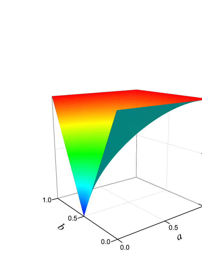
Figure 6: (Color online) Energy gap between the ground and the first excited states of the Hamiltonian $H_{i}$ as a function of $a$ and $b$.

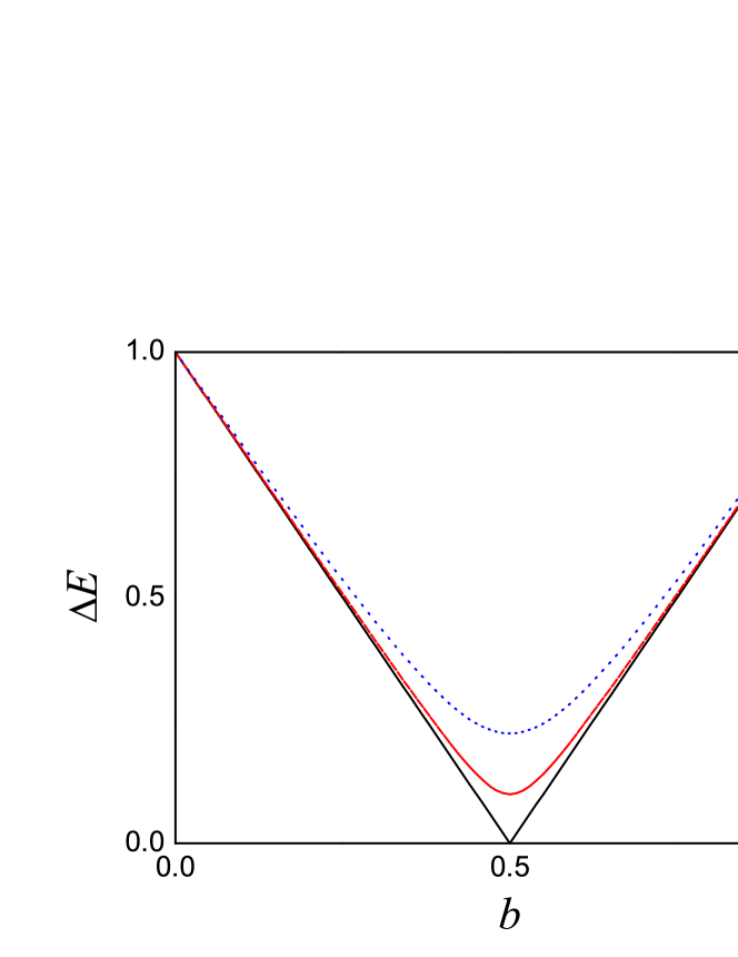
Figure 7: (Color online) Energy gap between the ground and the first excited states of the Hamiltonian $H_{i}$ as a function of $b$ by setting $a=0,0.01,0.05$, respectively.

In our algorithm, $M_{i}$ is an approximate estimation of $N_{i}$ by using Monte Carlo sampling. Let $b=a+\delta$, where $\delta$ is a small number, the energy gap can be expanded as

$$\Delta E = \sqrt{1-4a+8a^{2}-4a^{3}}-\frac{2\left(1-a\right)\left(1-2a\right)}{\sqrt{1-4a+8a^{2}-4a^{3}}}\delta$$ (50)

$$+\frac{2a\left(1-a\right)}{\left(1-4a+8a^{2}-4a^{3}\right)^{3/2}}\delta^{2}+O\left(\delta^{3}\right).$$

The first term has a minimum of $\sqrt{11}/3\sqrt{3}\approx 0.638$ at $a=1/3$.

Figure 8: Ratio $x_{1}^{(i)}/x_{2}^{(i)}$ between components $x_{1}^{(i)}$ and $x_{2}^{(i)}$ of the ground state of the Hamiltonian $H_{i}$.

($ii$) Evaluation of the overlap between the ground states of two adjacent Hamiltonians. Let $\mathbf{e}=\left(1,\cdots,1\right)^{\text{T}}$ and $\mathbf{0}=\left(0,\cdots,0\right)^{\text{T}}$ be $N_{i}\times 1$ vectors, respectively. The ground state of $H_{i}$ is $|V_{-}^{\left(i\right)}\rangle=x_{1}^{\left(i\right)}\left(\mathbf{e},0\right)^{\text{T}}+x_{2}^{\left(i\right)}\left(\mathbf{0},1\right)^{\text{T}}$, where $\left[x_{1}^{\left(i\right)}\right]^{2}+\left[x_{2}^{\left(i\right)}\right]^{2}=1$. The components $x_{1}^{\left(i\right)}$ and $x_{2}^{\left(i\right)}$ are in the following form:

$$x_{1}^{(i)}=\frac{1}{A}\left[\frac{1+\sqrt{\!1-4b-4ab^{2}+4b(a+b)}}{2b\sqrt{a\left(1-a\right)}}-\sqrt{\frac{1}{a}-1}\right].$$ (51)

and $x_{2}^{(i)}\!=\frac{1}{A}$, where $A=\sqrt{1+\left[\frac{1+\sqrt{1-4b-4ab^{2}+4b(a+b)}}{2b\sqrt{\!a\left(1-a\right)}}-\sqrt{\frac{1}{a}-1}\right]^{2}}$.

In basis $\left(\left\{|q_{i}\rangle\right\}_{q_{i}\in A_{i}}\text{, }|q_{i}^{\bot}\rangle\right)$, where $|q_{i}^{\bot}\rangle=\frac{1}{\sqrt{N-N_{i}}}\sum_{k\notin A_{i}}|k\rangle$, the state $|V_{-}^{\left(i\right)}\rangle$ can be written as:

$$|V_{-}^{\left(i\right)}\rangle\!=\!x_{1}^{\left(i\right)}\!\frac{1}{\sqrt{N_{i}}}\sum_{q_{i}\in A_{i}}|q_{i}\rangle+x_{2}^{\left(i\right)}\!\frac{1}{\sqrt{N-N_{i}}}\sum_{k\notin A_{i}}|k\rangle.$$ (52)

Correspondingly, the state $|V_{-}^{\left(i-1\right)}\rangle$ can be written as:

$$|V_{-}^{\left(i-1\right)}\rangle\! = \!x_{1}^{\left(i-1\right)}\!\frac{1}{\sqrt{N_{i-1}}}\sum_{q_{i-1}\in A_{i-1}}|q_{i-1}\rangle+x_{2}^{\left(i-1\right)}\!\frac{1}{\sqrt{N-N_{i-1}}}\sum_{k\notin A_{i-1}}|k\rangle$$ (53)

$$= \!x_{1}^{\left(i-1\right)}\!\frac{1}{\sqrt{N_{i-1}}}\left(\sum_{k\in A_{i-1}\setminus A_{i}}|k\rangle+\sum_{k\in A_{i}}|k\rangle\right)+x_{2}^{\left(i-1\right)}\!\frac{1}{\sqrt{N-N_{i-1}}}\sum_{k\notin A_{i-1}}|k\rangle.$$

Thus the overlap between the ground states $|V_{-}^{\left(i-1\right)}\rangle$ and $|V_{-}^{\left(i\right)}\rangle$ is

$$g_{0}^{(i)}\! = \!\langle V_{-}^{\left(i\!-\!1\right)}|V_{-}^{\left(i\right)}\rangle\!=\!\sqrt{\!\frac{N_{i}}{N_{i-1}}}x_{1}^{\left(i\!-\!1\right)\ast}x_{1}^{\left(i\right)}\!+\!\frac{N_{i\!-\!1}\!-\!N_{i}}{\sqrt{\!N_{i\!-\!1}\!(N\!-\!N_{i})}}x_{1}^{\left(i\!-\!1\right)\ast}x_{2}^{(i)}\!+\!\sqrt{\frac{N\!-\!N_{i\!-\!1}}{N\!-\!N_{i}}}x_{2}^{\left(i\!-\!1\right)\ast}x_{2}^{\left(i\right)}.$$ (54)

By setting $b=a+\delta$, the ratio $x_{1}^{(i)}/x_{2}^{(i)}$ can be expanded as

$$x_{1}^{(i)}/x_{2}^{(i)} = \frac{-2a+2a^{2}+1+\sqrt{\!1-4a+8a^{2}-4a^{3}}}{2a\sqrt{a\left(1-a\right)}}+\frac{-1\!+\!2a\!-\!2a^{2}\!-\!\sqrt{1\!-\!4a\!+\!8a^{2}\!-\!4a^{3}}}{2a^{2}\!\sqrt{a\left(1\!-\!a\right)}\!\sqrt{\!1-\!4a\!+\!8a^{2}\!-\!4a^{3}}}\delta\!+\!O\left(\delta^{2}\right).$$ (55)

The first term of the above expansion is shown in Fig. $8$, which has a minimum of $2.21$ at $a=\left(3-\sqrt{3}\right)/2$.

In order to make the overlap $g_{0}^{(i)}$ not to be exponentially small, we require that $x_{1}^{\left(i\right)}>x_{2}^{\left(i\right)}$, such that the overlap $g_{0}^{(i)}$ is guaranteed to be polynomial large when the ratio $N_{i-1}/N_{i}$ is polynomial large. This can be achieved by setting $M_{i}$ or $b$ appropriately. By solving the inequality $x_{1}^{\left(i\right)}>x_{2}^{\left(i\right)}$, we have $b<\frac{1}{2\left(1-a\right)}$, which also can be written as $2M_{i}\left(N-N_{i}\right)<N^{2}$. Both $M_{i}$ and $N_{i}$ are in decreasing order with the increasing of the steps of the algorithm, therefore the condition is easily satisfied in the last few steps of the algorithm. While at the beginning steps, $N_{i}$ can be obtained approximately by using the Monte Carlo sampling. Then we can set $M_{i}$ accordingly to satisfy the condition.

Summarizing the above calculation results, we find that the parameters $M_{i}$ should be set such that: the point $\left(a,b\right)$ should be far away from the neighborhood of the point $\left(0,1/2\right)$, and $2M_{i}\left(N-N_{i}\right)<N^{2}$.

References

- (1) T. Weise, Global Optimization Algorithms – Theory and Application. (Thomas Weise, University of Kassel, Germany, 2007).
- (2) S. Boyd, L. Vandenberghe, Convex Optimization, (Cambridge University Press, 2004).
- (3) J. Nocedal, S. J. Wright, Numerical Optimization, (Springer, 2006).
- (4) R. Fletcher, Practical Method of Optimization. (2nd Edition, Wiley, New York, 1987).
- (5) C. Floudas and C. Gounaris, A review of recent advances in global optimization, J. of Glob. Optim., 45, 3 (2009).
- (6) E. Farhi, J. Goldstone, S. Gutmann and M. Sipser, Quantum computation by adiabatic evolution, ArXiv:quant-ph/0001106.
- (7) A. Finnila, M. Gomez, C. Sebenik, C. Stenson, and J. Doll, Chem. Phys. Lett., 219, 343 (1994).
- (8) T. Kadowaki and H. Nishimori, Phys. Rev. E, 58, 5355 (1998).
- (9) J. Brooke, D. Bitko, T. Rosenbaum, and G. Aeppli, Science, 284, 779 (1999).
- (10) G. Santoro, R. Martoňák, E. Tosatti, and R. Car, Science, 295, 2427 (2002).
- (11) M. Johnson, et al. Quantum annealing with manufactured spins, Nature, 473, 194 (2011).
- (12) E. Farhi, J. Goldstone, and S. Gutmann. A Quantum Approximate Optimization Algorithm, ArXiv: 1411.4028.
- (13) J. Preskill, Quantum Computing in the NISQ era and beyond, Quantum 2, 79 (2018).
- (14) S. Jordan, Fast quantum algorithm for numerical gradient estimation Phys. Rev. Lett., 95, 050501 (2005).
- (15) P. Rebentrost, M. Schuld, L. Wossnig, F. Petruccione and S. Lloyd, Quantum gradient descent and Newton’s method for constrained polynomial optimization, New J. Phys. 21, 073023 (2019).
- (16) L. Grover, QuantumMechanics Helps in Searching for a Needle in a Haystack, Phys. Rev. Lett. 79, 325 (1997).
- (17) C. Dürr and Peter Høyer. A quantum algorithm for finding the minimum, arXiv: quant-ph/9607014.
- (18) V. Protopopescu and J. Barhen. Solving a Class of Continuous Global Optimization Problems using Quantum Algorithms. Physics Letters A, 296, 9 (2002).
- (19) D. Bulger, W. Baritompa, and G. R. Wood. Implementing pure adaptive search with grover’s quantum algorithm. Journal of Optimization Theory and Applications, 116, 517 (2003).
- (20) W. Baritompa, D. Bulger, and G. Wood. Grover’s quantum algorithm applied to global optimization. SIAM J. on Optimization, 15, 1170 (2005).
- (21) L. A. B. Kowada, C. Lavor, R. Portugal, and C. H. Figueiredo, Int. J. of Quant. Inf. 6, 427 (2008).
- (22) Y. Liu and G. J. Koehler, Eur. J. of Operational Research, 207, 620 (2010); J. of Glob. Optim. 52, 607 (2011).
- (23) A. Gilliam, S. Woerner and C. Gonciulea, Grover Adaptive Search for Constrained Polynomial Binary Optimization, Quantum 5, 428 (2021).
- (24) H. Wang, S. Yu and H. Xiang, Efficient quantum algorithm for solving structured problems via multistep quantum computation, Phys. Rev. Res. 5, L012004 (2023).
- (25) H. Wang, Quantum algorithm for obtaining the eigenstates of a physical system, Phys. Rev. A 93, 052334 (2016).
- (26) Z. Li, et al., Quantum simulation of resonant transitions for solving the Eigenproblem of an effective water Hamiltonian, Phys. Rev. Lett. 122, 090504 (2019).
- (27) W. K. Wootters and W. H. Zurek, A single quantum cannot be cloned, Nature, 299, 802 (1982).
- (28) D. Dieks, Communication by EPR devices, Phys. Lett. A, 92, 271 (1982).
- (29) M. A. Nielsen and I. L. Chuang, Quantum computation and quantum information. (Cambridge Univ. Press, Cambridge, England, 2000).
- (30) J. M. Martyn, Z. M. Rossi, A. K. Tan and I. L. Chuang, Grand unification of quantum algorithms, PRX Quantum, 2, 040203 (2021).
- (31) F. Wang and D. P. Landau, Phys. Rev. Lett. 86, 2050 (2001).
- (32) C. Cohen-Tannoudji, B. Diu, and F. Laloë, Quantum Mechanics Vol. 1, p414, (Wiley-Interscience Publication 1977).
- (33) http://www.infinity77.net/global_optimization /test_functions.html.