Recurring Auctions with Costly Entry:
Theory and Evidence

Abstract

Recurring auctions are ubiquitous for selling durable assets like artworks and homes, with follow-up auctions held for unsold items. We investigate such auctions theoretically and empirically. Theoretical analysis demonstrates that recurring auctions outperform single-round auctions when buyers face entry costs, enhancing efficiency and revenue due to sorted entry of potential buyers. Optimal reserve price sequences are characterized. Empirical findings from home foreclosure auctions in China reveal significant annual gains in efficiency (3.40 billion USD, 16.60%) and revenue (2.97 billion USD, 15.92%) using recurring auctions compared to single-round auctions. Implementing optimal reserve prices can further improve efficiency (3.35%) and revenue (3.06%).

Keywords:

recurring auctions, auction design, sorting, entry.

JEL Classification Codes:

D44, D82, R31.

1 Introduction

Auctions for durable assets like houses and artworks are commonly recurring: a subsequent auction will often be held if the initial one fails to sell the item. Despite the prevalence of recurring auctions, there has been limited scholarly effort to understand why they exist, let alone their equilibrium properties. One possible explanation for their existence is that sellers are subject to limited commitment: they cannot commit to withholding the item for sale forever after a failed auction. However, this cannot be the whole story: if a single-round auction is indeed optimal, there are many ways to address the limited commitment problem. For example, sellers can build a reputation of no follow-up auctions by donating unsold items to charity when auctions fail. Moreover, in many high-stake auctions of valuable assets or resources, the government acts as the seller, and limited commitment may be less of an issue.

In this paper, we provide both a theoretical model and an empirical analysis of recurring auctions. By showing that recurring auctions can outperform single-round mechanisms in both efficiency and revenue, and by evaluating the related gains in an empirical setting, we offer a new explanation for the ubiquity of such mechanisms. Our analyses also shed light on how to fine-tune recurring auctions to further promote efficiency and revenue.

Recurring and single-round auctions may differ significantly because entry costs are often important in the real world. For example, it may take time and effort to qualify as a bidder and prepare a bid. In particular, a deposit is often required in auctions for valuable assets, which imposes a liquidity cost on the bidder. However, participation costs are usually assumed away in the auction design literature. This leads to a biased prediction in terms of efficiency maximization, as the social cost of entry is neglected. Failing to account for entry costs may also mislead the revenue-maximizing design.

In an equilibrium model, we show that recurring auctions outperform single-round auctions in efficiency and revenue when entry is costly for potential buyers. Our model setup is as follows. We consider an independent private value environment with costly entry. Specifically, a seller has one item for sale, and there is a fixed pool of potential buyers whose values are independently drawn from the same distribution. The seller holds auctions in a recurring way: if an auction fails, either because no bidder shows up or because the reserve price is not met, she will hold a follow-up auction in the next period, until some time limit is reached. Potential buyers decide whether to incur an entry cost to participate in an auction and become a bidder, as time progresses. To align with our empirical context, where the majority of the entry cost comes from the financial constraints and the eligibility screening process, we assume that potential buyers know their private values before they make entry decisions. We characterize the equilibrium of the recurring auction game with any arbitrary time limit and reserve price sequence.

The intuition for recurring auctions’ dominance is straightforward: in a recurring auction, potential buyers sort their timing of entry according to their private values for the item. Strong potential buyers (who have high values) tend to enter early, while weak potential buyers (who have low values) tend to wait until they have a good chance of winning. This is because strong potential buyers lose more from waiting, and weak potential buyers’ entry costs are more likely wasted if they enter early.

The sorted entry pattern increases the expected total surplus in two ways. First, it reduces the probability that two or more bidders simultaneously incur the entry cost, and thereby reduces waste. In particular, weak potential buyers wait until they are sure that others are not too strong either, and then enter into the auction. This way, their entry costs are less often incurred and wasted in early rounds. Second, it increases the probability that the item is ultimately sold. When an auction fails, the potential buyers update their beliefs about the others’ private values. In late rounds, they infer that the market is less competitive, as no potential rivals had high enough values to enter in previous rounds. This encourages them to enter into the auction, which reduces the likelihood that the item goes unsold. Because of these two benefits, recurring auctions with appropriately chosen reserve prices always generate higher expected total surplus than single-round auctions (Theorem 1). Similarly, we obtain a revenue dominance result (Theorem 2).

We then derive the optimal sequence of reserve prices in a recurring auction. If the seller aims to maximize efficiency, she trades off between making a marginal potential buyer enter at time $t$ or at time $t+1$. Consider the thought experiment where the marginal potential buyer enters at time $t+1$ instead of time $t$. Then there is a social gain as the marginal potential buyer’s entry cost is less often incurred, because his entry is conditional on no entry by other potential buyers at time $t$. However, there are also two kinds of social loss. First, there is a loss from discounting as the item may be allocated one period later. Second, entry at time $t+1$ by other potential buyers could have been avoided had the marginal potential buyer entered at time $t$. In the optimum, the choice of reserve prices equalizes the social gain and loss from making a marginal potential buyer enter at time $t+1$ instead of time $t$ (Theorem 3). If the seller aims to maximize profit, she faces a similar tradeoff, and the optimal reserve prices can be characterized accordingly (Theorem 4). In particular, the profit-maximizing condition can be obtained by replacing the marginal potential buyer’s value with his virtual value in the efficiency-maximizing condition. This is intuitive, as we know from the mechanism design literature that the virtual value accrues to the seller while the value contributes to social surplus.

Given the theoretical results, it is natural to ask the following quantitative questions in an empirical setting: (i) What are the magnitudes of the efficiency gain and the revenue gain from using a recurring auction relative to a single-round auction? (ii) How much can efficiency and revenue be improved for recurring auctions in practice?

We apply our theory to home foreclosure auctions in China, which represent a significant market. In 2019, over 118,000 foreclosed houses were transacted with a transaction volume of 28 billion USD. The market size continues to grow at a high speed due to high levels of leverage in the country’s real estate sector. Using home foreclosure auction data in Fujian province from 2017 to 2019, we estimate structural parameters in a recurring auction model. The data attest to the important features in our theoretical model setup: up to three auctions were held in a row for a foreclosed property; the failure rate of the initial auctions was high (38%), while only 7% of the foreclosed homes went unsold after all the follow-up auctions; and entry costs were considerable due to the financial constraints and the eligibility screening process.

Using simulated maximum likelihood with importance sampling (Ackerberg, 2009), our structural estimation comprises two steps. First, for each auction round and each simulation, we solve for the equilibrium entry thresholds using the intertemporal indifference conditions. Second, we calculate the likelihood using the entry thresholds and observable auction outcomes. Our results suggest that intertemporal considerations play an important role in potential buyers’ entry decisions, which affirms the necessity of incorporating dynamics in the empirical analysis.

Our counterfactual analyses support the theoretical predictions: compared to single-round auctions with the same (first-period) reserve price, the recurring auctions raise the annual efficiency by 3.40 billion USD (16.60%) and revenue by 2.97 billion USD (15.92%) in China’s home foreclosure market. Using the optimal reserve price sequences derived from our model can further improve efficiency by 0.80 billion USD (3.35%) and revenue by 0.66 billion USD (3.06%), respectively. Most of the efficiency and revenue gain is realized by holding a two-round recurring auction. Increasing the recurring auction rounds from 2 to 3 has a relatively small impact on the auction outcome.

This paper contributes to the literature on mechanism design with costly entry. Stegeman (1996) investigates efficiency-maximizing mechanisms in an independent private value (IPV) setting with costly entry. Lu (2009) and Celik and Yilankaya (2009) study revenue-maximizing mechanisms within the same framework. These studies all focus on single-round mechanisms in the sense that messaging and allocation happen within the same period. This single-round assumption is innocuous with free entry. However, it misleads the auction design when entry is costly. Notably, in the single-round mechanism design problem, it is impossible for the potential buyers to acquire any information about others’ values before deciding whether to enter, because the mechanism only assigns allocation conditional on entry. This paper complements the existing literature by incorporating the time dimension and considering a dynamic auction setting. We demonstrate how sorted entry emerges in recurring auctions, which allows potential buyers to update their beliefs about competitors’ values and make more efficient entry decisions. McAfee and Vincent (1997), Skreta (2015), and Liu et al. (2019) also consider auction games with the possibility of follow-up auctions. However, they abstract away from entry costs and focus on the implications of limited seller commitment on the reserve price sequence and optimal auction design.

A voluminous literature theoretically studies auctions with costly entry. One strand of the literature, interpreting entry costs as information acquisition costs, assumes that potential buyers are uninformed of their values when they make entry decisions (e.g., Levin and Smith, 1994; Burguet and Sakovics, 1996). Another strand of literature focuses on the costs of preparing bids or obtaining eligibility and assumes that potential buyers are fully informed of their values (e.g., Samuelson, 1985; McAdams, 2015). Recently, a growing literature combines the two modeling approaches and allows potential buyers to receive an arbitrarily informative signal before deciding whether to enter (Roberts and Sweeting, 2013; Gentry et al., 2017). The current paper follows the second strand of literature and considers fully informed entry, which seems plausible in our empirical application.

The existing literature typically focuses on single-round auctions. The only exception we know is Burguet and Sakovics (1996), where the authors consider two-period recurring auctions while assuming uninformed entry and no discounting. Because potential buyers do not know their values, the sorted entry pattern does not appear, and the benefit that weak potential buyers wait to avoid wasting entry costs does not exist. Still, an encouraging entry effect exists in the second round because potential buyers infer that first-round entrants have bad draws upon observing auction failure. Due to this effect, the authors conclude that a recurring auction can generically achieve greater efficiency and higher revenue than a single-round auction. In the informed entry case, the current paper demonstrates two benefits of the recurring auction, as mentioned previously. We establish the efficiency and revenue dominance result and provide a complete characterization of optimal reserve price sequences with any number of auction rounds and any discount rate.

Previous studies have considered other types of dynamics in auction games with costly entry. Ye (2007) and Quint and Hendricks (2018) analyze auction games where an indicative bidding round precedes the actual auction to screen potential buyers. McAdams (2015) studies sequential costly bidding in a second-price auction. Bulow and Klemperer (2009) and Roberts and Sweeting (2013) also consider sequential costly bidding but fix the order in which potential buyers move.

We contribute to the empirical literature in two ways. First, we introduce and study a new dynamic setting where multiple auctions can be held across time for the same item. To our knowledge, this is the first empirical study to incorporate the possibility of follow-up auctions upon auction failure. Building upon previous research on single-round auction estimation (Laffont et al., 1995; Guerre et al., 1995; Guerre et al., 2000; Hortaçsu and Perrigne, 2021), this paper proposes a framework for estimating recurring auctions with costly entry. Our findings suggest that ignoring the dynamics when auctions are recurring can result in underestimating bidders’ value distribution and overestimating entry costs. This is because the single-round model overlooks potential buyers’ self-selection across time and incorrectly attributes low transaction prices in late auction rounds to low values and high entry costs.

While a plethora of auction dynamics has been explored by the theoretical literature, related empirical studies remain scarce, and most of them focus on repeated sales or procurement of homogeneous items. In the repeated highway procurement setting, Jofre-Bonet and Pesendorfer (2000, 2003) and Groeger (2014) empirically investigate the effects of backlog or experience on bidders’ behavior. Jeziorski and Krasnokutskaya (2016) point out that subcontracting allows suppliers to control their capacities more flexibly and thus alleviates dynamic concerns.

Second, we contribute to the literature by structurally analyzing the foreclosure market. Despite being a sizable market with rapidly growing transaction volumes, it has received little attention in the literature. This paper represents one of the first attempts to utilize a structural approach in this market. Our structural estimation affords a wide variety of counterfactual analyses and thus helps inform better designs to promote important social objectives.

The remainder of this paper proceeds as follows: Section 2 lays out the recurring auction model and discusses the single-round benchmark. Section 3 provides some illustrative examples and the theoretical results. Section 4 discusses the data and institutional background of home foreclosure auctions and presents descriptive evidence. Section 5 proposes an empirical framework to estimate the recurring auction model. Section 6 presents the estimation results. Section 7 shows the counterfactual analyses. Section 8 concludes the paper. All proofs are relegated to Appendix A.

2 Model

A seller has one item for sale, and her value for the item is $v_{s}$. There are $N$ potential buyers, indexed by the set $\mathcal{N}:=\{1,2,\ldots,N\}$. Each potential buyer $n\in\mathcal{N}$ has a private value $v_{n}$ for the item. The values of the potential buyers are independently and identically distributed on the interval $[\underline{v},\overline{v}]$ according to the cumulative distribution function $F(\cdot)$. The seller holds an English auction or possibly a sequence of English auctions to sell the item. We focus on English auctions for ease of exposition and to be consistent with the empirical application, in which the data is from open-outcry auctions. However, it is worth noting that a revenue equivalence can be established in the current setting, so our results hold for all standard auction formats. Participation or entry in an auction is costly for potential buyers. The entry cost is $K>0$. Potential buyers know their values at the time they make entry decisions. It is natural to require that $v_{s}<\overline{v}-K$.

The timing of the auction game is as follows. An auction is held at time $t=1$. If no buyer shows up and an auction fails at time $t$, the seller will hold another auction at time $t+1$ until time $T\geq 1$, after which the seller keeps the item forever. Before the game starts, the seller sets a reserve price sequence $\bm{r}:=(r_{t})_{1\leq t\leq T}$, where $r_{t}$ is the reserve price in the auction (possibly) held at time $t$. If $T=1$, we have a single-round auction; if $T>1$, we refer to the auction as a recurring auction.

While paying the entry cost grants a potential buyer access to the current and all subsequent auctions, in equilibrium, the potential buyer always participates immediately in the current auction (and bids above the reserve price) after incurring the entry cost. Consequently, whenever someone enters, the item is sold in the current period and there is no continuation game. At the beginning of each period, if an auction is held, implying no one had entered previously, the potential buyers simultaneously and independently decide whether to incur an entry cost of $K$ to participate in the auction. If any potential buyers choose to enter, the auction begins and a price clock ascends continuously from the reserve price. The price clock continues to ascend so long as two or more bidders remain in the auction and stops when all but one have dropped out. The last bidder remaining in the auction wins the item at the final clock price, and the auction game ends. If no one enters, the game proceeds to the next period or ends if this is the last period $T$.

The common discount factor for the seller and potential buyers is $\delta\in(0,1)$. As long as the item has not been sold, the seller derives a flow utility $(1-\delta)v_{s}$ from the item in each period. Everything described above, apart from potential buyers’ private values, is common knowledge.

For the equilibrium analysis, which will be detailed in the next section, it is useful to note that, conditional on participation, bidding truthfully is the best a bidder can do in both the single-round auction and the recurring auction. Therefore, throughout the paper, we focus on equilibria in cutoff strategies, under which a potential buyer participates and bids his value if and only if his value is above a cutoff. Given that the potential buyers are ex-ante symmetric, we further restrict our attention to the symmetric equilibrium of the auction game, where the entry thresholds are identical for the potential buyers.

Assumption 1 (Symmetric Equilibrium in Cutoff Strategies)

Throughout the paper, unless otherwise mentioned, we focus on symmetric equilibria in cutoff strategies.

We take the single-round auction as a benchmark since it performs well in terms of both efficiency and revenue. Celik and Yilankaya (2009) point out that the single-round auction, with an appropriately chosen reserve price, is optimal among all symmetric single-round mechanisms. That is, with an appropriately chosen reserve price, the single-round auction can maximize either the efficiency or the seller’s expected profit. Moreover, the authors provide conditions under which the single-round auction is optimal among all single-round mechanisms, symmetric or not.

Notably, a disadvantage of the single-round auction, or any other single-round mechanism, is that potential buyers cannot learn anything about their rivals’ values before making entry decisions. This foreshadows an efficiency loss in wasteful entry. In contrast, the recurring auction incorporates the time dimension, which allows potential buyers to make dynamic entry decisions. As such, potential buyers have the opportunity to update their beliefs about others’ realized values and to economize on their entry decisions. For example, if a potential buyer observes that no one has participated in the previous periods, he would infer that others do not have high values for the item and thus feel more confident about entry into the auction. This comparison underlies the superior performance of the recurring auction. We elaborate more on this point in the following section.

3 Illustrative Examples and Equilibrium Analysis

3.1 Illustrative Examples

Before we analyze the general model in detail, it would be beneficial to demonstrate the main insights through simple examples.

Example 1

There are $N=2$ potential buyers whose values are independently and identically drawn from the uniform distribution on $[0,1]$. The seller’s value is $v_{s}=0$. A potential buyer’s entry cost is $K=0.2$. The common discount factor is $\delta=0.97$.

In this example, there is a unique equilibrium of the single-round auction with no reserve price (Tan and Yilankaya, 2006). In the equilibrium, the potential buyers use a cutoff entry strategy: potential buyer $n$ participates and bids $v_{n}$ in the auction if and only if $v_{n}\geq 0.45$. This equilibrium maximizes the expected total surplus among all single-round mechanisms (Stegeman, 1996). The expected total surplus in this case is 0.39.

Now consider a two-period recurring auction (i.e., $T=2$) with a reserve price sequence $(r_{1},r_{2})=(0.14,0)$. By 1, to characterize the equilibrium, we only need to pin down entry thresholds. Intuitively, a strong potential player (who has a high realized value) tends to enter early while a weak player tends to wait, because: (i) the strong player loses more if he waits and the item is bought by other potential buyers, he also loses more to discounting if he wins in the next period as compared with winning now; and (ii) the weak player has a lower chance of winning in the current period, which means the entry cost is more likely wasted. We therefore consider the following cutoff equilibrium structure: potential buyers whose values are above $v_{1}^{*}$ enter in the first period; those with values in between $v_{1}^{*}$ and $v_{2}^{*}$, with $v_{2}^{*}\leq v_{1}^{*}$, enter in the second period; and those whose values fall below $v_{2}^{*}$ never enter. The entry cutoffs can be pinned down by the indifference conditions of the marginal potential buyers. The idea is that a potential buyer with a cutoff value should be indifferent between entering now or in the next period (or, if the current period is the last period, not entering at all). In Example 1, we have that $(v_{1}^{*},v_{2}^{*})=(0.66,0.36)$. The expected total surplus in this case is 0.42, which is higher than that in the single-round auction.

To understand the reason behind the comparison in efficiency, it is useful to note that the recurring auction allows the potential buyers to sort their entry over time. This provides an opportunity for the players to condition their entry on some information they can obtain about potential rivals. Sorting brings about two benefits to the total surplus: First, weak potential buyers can wait until they are sure that others are not too strong either, and then enter into the auction. This way, their entry costs are wasted less often. We refer to this as the economizing on entry benefit. Second, when an auction fails, the potential buyers update their beliefs about the others. They infer that the market is less competitive, as no potential rivals have a high enough value to enter in the previous period. So they would be encouraged to enter into the auction, which reduces the possibility that the item goes unsold. This is reflected by the fact that the entry threshold in the single-round auction (0.45) is higher than the entry threshold in the recurring auction at $t=2$ (0.36). In the single-round auction, the item remains unsold with a probability of 0.2; whereas in the recurring auction, the probability is reduced to 0.13. We refer to this as the reducing auction failure benefit.

We use Figure 1 to visualize the two benefits mentioned above. Figure 1(a) shows the entry decisions in the single-round auction. When both potential buyers’ values are above the entry cutoff 0.45, there is excessive entry: The ex post efficiency would be maximized if the strong potential buyer is the only participant. The value profiles corresponding to excessive entry are reflected by the shaded area in the upper right corner. When both potential buyers’ values are below the entry cutoff, but one of the potential buyers has a value higher than the entry cost (the shaded area close to the lower left corner), there is no entry, which is not efficient: the total surplus would be raised if the strong potential buyer were to enter. In all the other unshaded areas, (no) entry is efficient in equilibrium. We similarly plot the efficient and inefficient areas in terms of entry for the recurring auction in Figure 1(b). Because players sort their entry over time, both the areas of excessive entry and inefficient no entry are much smaller as compared with the single-round auction case. The difference between the excessive entry areas reflects the economizing on entry benefit, and the difference between the inefficient no entry areas reflects the reducing auction failure benefit.

Figure 1: Equilibrium Entry in Recurring and Single-Round Auctions.

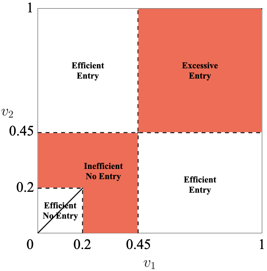
(a) Entry in the Single-Round Auction.

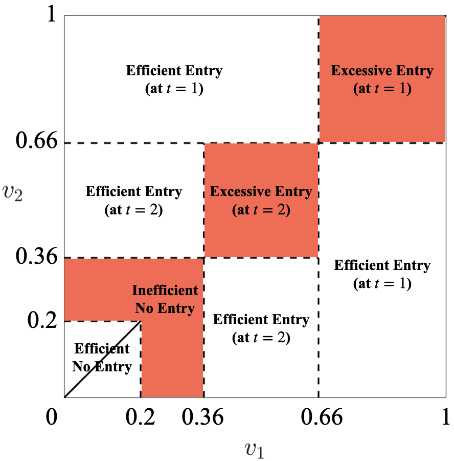
(b) Entry in the Recurring Auction.

Notably, as is pointed out by Samuelson (1985), setting the reserve price equal to the seller’s valuation maximizes the expected total surplus in the single-round auction. In contrast, to maximize efficiency in the recurring auction, a non-trivial reserve price at $t=1$ would be used in the recurring auction. This is because the first-period reserve price affects the extent of sorting. If $r_{1}$ is 0, too many potential buyers would participate in the first period, and this reduces the informativeness of observing whether or not the first auction has failed. As a result, the gain from sorting is not maximized. In Figure 1(b), varying $r_{1}$ effectively changes the entry threshold in the first period and thus the areas of the two shaded squares. If the entry threshold is too low (resp. too high), the excessive entry at $t=1$ (resp. $t=2$) area will grow too big and squeeze out the economizing on entry benefit.

Figure 2 plots how the maximized efficiency (by varying reserve prices) changes along with the total number of periods. Compared to the single-round auction, the 6-period recurring auction increases efficiency by around 11% of the first-best efficiency level, given by $\mathbf{E}\{\max_{n\in\mathcal{N}}[\max(v_{n}-K-v_{s},0)]\}$. It is clear that the value of having one more auction or period diminishes over time. The majority of the efficiency improvement over the single-round auction is realized after having the second and the third period.

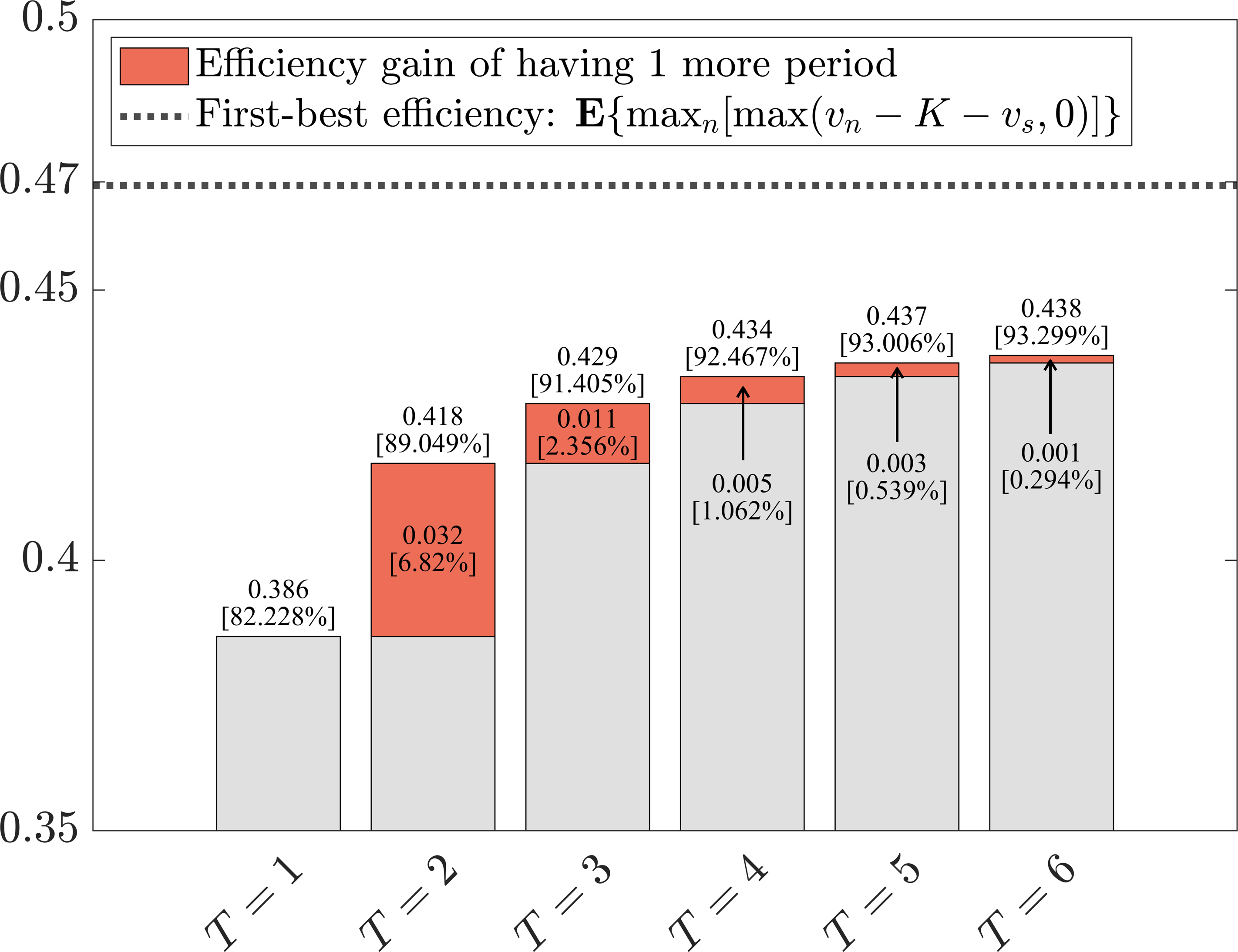
Figure 2: Maximized Expected Total Surplus in Single-Round and Recurring Auctions While Varying $T$.

Notes: The numbers above the bars (and not in the square brackets) are the values of maximized expected total surplus in the auctions, and the numbers in the square brackets are those values as a percentage of the full efficiency. The numbers in or pointing to the upper (red) parts of the bars are the efficiency gain of extending the auction game for 1 more period. Again, the numbers in the square brackets are those values as a percentage of the full efficiency.

Next, we consider the revenue comparison between the revenue-maximizing single-round mechanism and the recurring auction. Because the recurring auction outperforms single-round mechanisms in terms of efficiency, one might expect the recurring auction (with appropriately chosen reserve prices) to also generate more revenue for the seller. After all, the seller’s revenue is part of the total surplus. Celik and Yilankaya (2009) set up the single-round mechanism design problem with costly entry and study revenue maximization. From their results, it follows that a second-price auction with a reserve price of 0.35 maximizes the revenue across all single-round mechanisms in Example 1. The maximized revenue is 0.25. In contrast, with the reserve price sequence set to $(r_{1},r_{2})=(0.4,0.37)$, the recurring auction generates a revenue of 0.26.

Finally, we briefly discuss another example to further illustrate the recurring auction’s efficiency dominance over the single-round auction. With costly entry, it is well-known that the efficiency may not be monotonically increasing in the number of potential buyers (Samuelson, 1985). This is because, with more potential buyers, each potential buyer worries more about prospective competition and is more inclined to skip the auction to save entry costs. We demonstrate that recurring auctions can reverse this counterintuitive result using the following example taken from Stegeman (1996).

Example 2

There are $N\geq 1$ potential buyers whose values are independently and identically drawn from the uniform distribution on $[1,2]$. The seller’s value is $v_{s}=0$. A potential buyer’s entry cost is $K=0.3$. The common discount factor is $\delta=0.97$.

The diamond markers in Figure 3 show how the expected total surplus in the single-round auction changes with the number of potential buyers. It can be seen that the efficiency actually decreases with more potential buyers. This reflects that coordinating and economizing on entry is difficult in a single-round setting. Without coordination, the prospect of excessive competition distorts entry and harms efficiency. The triangle and circle markers show the maximized expected total surplus (across all reserve price sequences) in 2- and 3-period recurring auctions, respectively. As the potential buyers sort their entry over time in recurring auctions, the efficiency is monotonically increasing in the number of potential buyers.

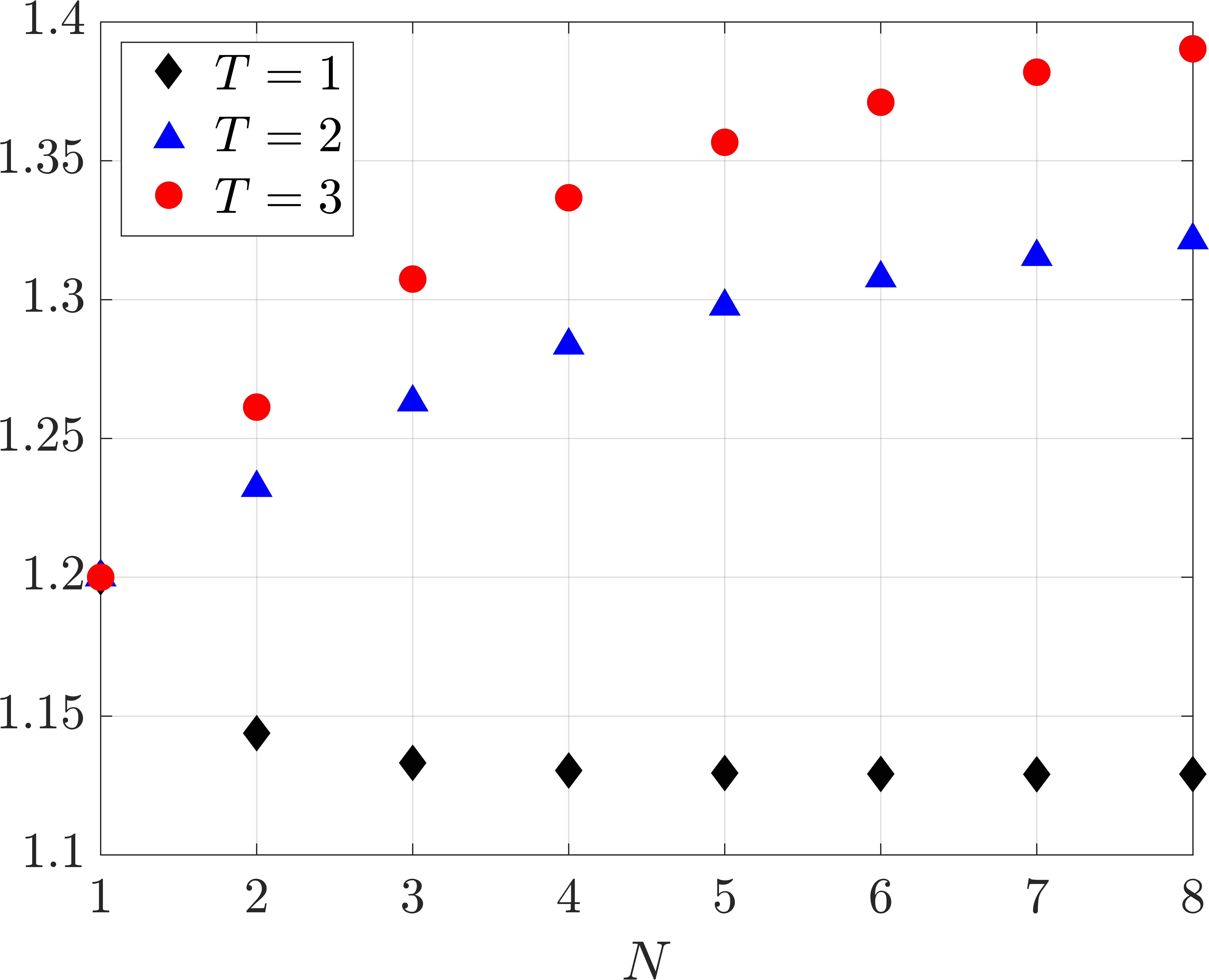
Figure 3: Maximized Expected Total Surplus in Single-Round and Recurring Auctions While Varying $N$.

Stegeman (1996) points out that coordination may happen in single-round auctions in the form of asymmetric equilibria. Consider the $N=2$ case: apart from the symmetric equilibrium where a potential buyer enters if his value is above 1.24, there is also an asymmetric equilibrium where one bidder always enters and the other enters if his value is above 1.77. The expected total surplus is 1.22 in the asymmetric equilibrium, which is greater than that in the symmetric equilibrium, 1.20. However, relying on asymmetric equilibria to coordinate entry and improve efficiency is precarious, as an asymmetric equilibrium need not always exist. Moreover, coordination in the form of asymmetric equilibrium may not be very effective as compared with the sorted entry pattern in recurring auctions. As Figure 3 shows, in the $N=2$ case, the efficiencies in the 2- and 3-period recurring auctions are 1.23 and 1.26, respectively.

In a similar vein, Celik and Yilankaya (2009) and Lu (2009) provide examples where asymmetric equilibria in single-round auctions generate higher expected revenue for the seller. However, these improvements are insignificant and once dynamics are incorporated, the symmetric equilibria in recurring auctions lead to much more sizable improvements.^,

3.2 Equilibrium Analysis

We now proceed to the formal analysis of the model. For notational ease, we denote the CDF of the highest value among $N-1$ potential buyers by $G(\cdot)$. That is,

$$G(\cdot):=[F(\cdot)]^{N-1}.$$

Note that when bidders compete in an auction, there will be no continuation games as the item will be sold in the current period. As a result, truthful bidding is the best that a bidder can do conditional on entry. We focus on the symmetric Perfect Bayesian Equilibrium (PBE) with a cutoff structure of the recurring auction game. In equilibrium, potential buyers’ entry is governed by a sequence of cutoffs $\bm{v}^{*}:=(v_{t}^{*})_{1\leq t\leq T}$, where $v_{t}^{*}$ is the lowest type that will enter at time $t$ if an auction is held at that time (which implies all previous auctions have failed). Given that all the other potential buyers enter according to the cutoff strategy and bid truthfully upon entry, a type-$v$ potential buyer’s interim expected payoff from entering in the time-$t$ auction is given by $\Pi_{t}(v;\bm{v}^{*})/G(v_{t-1}^{*})$, where

$$\Pi_{t}(v;\bm{v}^{*})=\delta^{t-1}\left[\int_{v_{t}^{*}}^{\min\{\max\{v,v_{t}^{*}\},v_{t-1}^{*}\}}(v-x)dG(x)+(v-r_{t})G(v_{t}^{*})-G(v_{t-1}^{*})K\right].$$ (1)

We are now ready to characterize the symmetric PBE using the marginal potential buyers’ indifference conditions. Again, the idea is that a potential buyer with a cutoff type should be indifferent between entering in the current period or not.

Proposition 1 (Equilibrium Characterization)

A PBE is characterized by a sequence of (weakly) decreasing entry thresholds, $\bm{v}^{*}:=(v_{t}^{*})_{t=0}^{T}$, with $v_{0}^{*}:=\overline{v}$. In equilibrium, potential buyers with values between $v_{t-1}^{*}$ and $v_{t}^{*}$ enter at time $t$. If no period is skipped for sure—i.e., $v_{t-1}^{*}>v_{t}^{*}$ for all $1\leq t\leq T$—the entry thresholds solve the following indifference conditions: $\Pi_{t}(v_{t}^{*};\bm{v}^{*})=\Pi_{t+1}(v_{t}^{*};\bm{v}^{*})$, or equivalently,

$$G(v_{t}^{*})(v_{t}^{*}-r_{t})-KG(v_{t-1}^{*})=\begin{cases}\delta\left[G(v_{t}^{*})(v_{t}^{*}-K)-\int_{v_{t+1}^{*}}^{v_{t}^{*}}xdG(x)-r_{t+1}G(v_{t+1}^{*})\right],&\text{ if }t<T,\\ 0,&\text{ if }t=T.\end{cases}$$ (2)

If some periods, say, the periods from $t_{0}$ to $t_{1}$, are skipped for sure, then the equilibrium conditions for these periods become

$$v_{t_{0}-1}^{*}=v_{t_{0}}^{*}=\ldots=v_{t_{1}}^{*}\text{ and }$$

$$\begin{cases}\Pi_{t_{0}-1}(v_{t_{0}-1}^{*};\bm{v}^{*})=\Pi_{t_{1}+1}(v_{t_{0}-1}^{*};\bm{v}^{*})\geq\max_{t_{0}\leq t\leq t_{1}}\Pi_{t}(v_{t_{0}-1}^{*};\bm{v}^{*}),&\text{ if }t_{0}>1;\\ \Pi_{t_{1}+1}(v_{t_{0}-1}^{*};\bm{v}^{*})\geq\max_{t_{0}\leq t\leq t_{1}}\Pi_{t}(v_{t_{0}-1}^{*};\bm{v}^{*}),&\text{ if }t_{0}=1.\end{cases}$$

Conditional on entry, bidders bid truthfully in the auction.

With the equilibrium characterization, we now compare the efficiency in recurring auctions and that in single-round auctions. Because of the economizing on entry benefit and the reducing auction failure benefit laid out in Section 3.1, the following efficiency dominance result can be obtained.

Theorem 1 (Efficiency Dominance)

Suppose that $N\geq 2$ and $K>0$. Then a recurring auction with an appropriately chosen reserve price sequence will achieve strictly higher efficiency than the symmetric equilibrium in any single-round auction.

Further, we show that the dominance of recurring auctions over single-round auctions also applies to the seller’s expected profit.

Theorem 2 (Revenue Dominance)

Suppose that $N\geq 2$ and $K>0$. Then a recurring auction with an appropriately chosen reserve price sequence will generate strictly higher profit for the seller than the symmetric equilibrium in any single-round auction.

3.3 Recurring Auction Design

In this part, we study the design of recurring auctions to maximize either efficiency or the seller’s profit. It is useful to note that the equilibrium conditions in Proposition 1 establish a mapping between reserve price sequences and the entry threshold sequences. The mapping allows us to reformulate the problem of choosing a reserve price sequence to that of choosing an entry threshold sequence. The reformulation will greatly simplify things, since it is generally infeasible to obtain an analytical solution of the entry threshold sequence given an arbitrary reserve price sequence, but the reverse is easy. In fact, an arbitrary entry threshold sequence $\bm{v}^{*}$ which is weakly decreasing can be induced by the reserve price sequence $\bm{r}(\bm{v}^{*})$, with $r_{t}(\bm{v}^{*})$ given by the following:

$$r_{t}(\bm{v}^{*})=\frac{1}{G(v_{t}^{*})}\left[\begin{array}[]{c}\sum_{\tau=t}^{T}(1-\delta)\delta^{\tau-t}G(v_{\tau}^{*})v_{\tau}^{*}-KG(v_{t-1}^{*})+\\ \sum_{\tau=t}^{T-1}\delta^{\tau-t+1}\int_{v_{\tau+1}^{*}}^{v_{\tau}^{*}}xdG(x)+\delta^{T-t+1}G(v_{T}^{*})v_{T}^{*}\end{array}\right].$$ (3)

We now present and solve the efficiency and revenue maximization problem with respect to entry thresholds.

Efficiency Maximization

Given a weakly decreasing entry threshold sequence $\bm{v}^{*}$, the expected total surplus in the recurring auction is

$$TS(\bm{v}^{*})=\sum_{t=1}^{T}\delta^{t-1}\bigg{\{}\int_{v_{t}^{*}}^{v_{t-1}^{*}}(x-v_{s})d[F(x)]^{N}-N[F(v_{t-1}^{*})]^{N-1}[F(v_{t-1}^{*})-F(v_{t}^{*})]K\bigg{\}}+v_{s},$$ (4)

where $\int_{v_{t}^{*}}^{v_{t-1}^{*}}(x-v_{s})d[F(x)]^{N}$ is the expected gain in allocative efficiency in period $t$, and the second term in the bracket is the expected entry cost in period $t$. The efficiency maximization problem is

$$\max_{\bm{v}^{*}}\leavevmode\nobreak\ TS(\bm{v}^{*})\leavevmode\nobreak\ \text{s.t.}\leavevmode\nobreak\ v_{t-1}^{*}\geq v_{t}^{*}\text{ for all }1\leq t\leq T.$$ (5)

The key to solving the problem is to show that the constraint $v_{t-1}^{*}\geq v_{t}^{*}$ does not bind. The reason that $v_{t-1}^{*}>v_{t}^{*}$ in the optimum can be seen by discussing two cases. First, if some final periods are skipped—i.e., $v_{t_{0}-1}^{*}>v_{t_{0}}^{*}=v_{t_{0}+1}^{*}=\ldots=v_{T}^{*}$ for some $t_{0}$—then the seller is effectively holding a single-round auction at time $t_{0}-1$, which cannot be efficient by Theorem 1. Second, if some periods other than the final periods are skipped—i.e., $v_{t_{0}}^{*}=v_{t_{0}+1}^{*}>v_{T}^{*}$ for some $t_{0}$—then the seller could in effect move every period after $t_{0}$ to one period earlier by using the entry threshold sequence $\bm{v}^{*^{\prime}}=(v_{1}^{*},\ldots,v_{t_{0}}^{*},v_{t_{0}+2}^{*},\ldots,v_{T}^{*},v_{T}^{*})$. This is more efficient than the original entry threshold sequence $\bm{v}^{*}$ since the efficiency gains in periods after $t_{0}$ are realized earlier. Having established that the constraint does not bind, the solution to (5) is characterized by the first-order conditions. Formally, we have the following result.

Theorem 3 (Efficient Recurring Auction)

Suppose the seller aims to maximize the expected total surplus by selecting a reserve price sequence of the recurring auction. Then in the efficient design, the equilibrium entry thresholds $\bm{v}^{*}$ solve the following:

$$\begin{cases}\left\{\left[\frac{F(v_{t-1}^{*})}{F(v_{t}^{*})}\right]^{N-1}-\delta\frac{NF(v_{t}^{*})-(N-1)F(v_{t+1}^{*})}{F(v_{t}^{*})}\right\}K-(1-\delta)(v_{t}^{*}-v_{s})=0,&\text{ if }t<T,\\ \left[\frac{F(v_{t-1}^{*})}{F(v_{t}^{*})}\right]^{N-1}K-(v_{t}^{*}-v_{s})=0,&\text{ if }t=T.\end{cases}$$ (6)

The corresponding reserve price sequence can be obtained from (3).

To see the intuition behind Theorem 3, let us consider the social gain and loss of making the marginal potential buyer with value $v_{t}^{*}$ enter at time $t+1$, instead of time $t$. The social gain manifests as saving in entry costs. Conditional on time $t$ is reached (i.e., no one has shown up in previous auction rounds), the cost of participating at time $t$ is $K$. However, if the marginal seller participates at time $t+1$, he incurs entry cost only if no one shows up at time $t$, so the expected entry cost is $\delta[F(v_{t}^{*})/F(v_{t-1}^{*})]^{N-1}K$. Consequently, the social gain of cost saving is $\{1-\delta[F(v_{t}^{*})/F(v_{t-1}^{*})]^{N-1}\}K$. The social loss consists of two parts. First, in the event that all the other potential buyers have values below $v_{t}^{*}$, there is a loss of allocating the item one period later. Specifically, the loss from discounting is $(1-\delta)[F(v_{t}^{*})/F(v_{t-1}^{*})]^{N-1}(v_{t}^{*}-v_{s})$. Second, if the marginal potential buyer had entered in period $t$, entry by other potential buyers in period $t+1$ could have been avoided. Since there are $N-1$ other potential buyers and the probability of each one of them entering in period $t+1$, conditional on period $t+1$ is reached, is $[F(v_{t}^{*})-F(v_{t+1}^{*})]/F(v_{t}^{*})$, the waste of period-$(t+1)$ entry is $\delta[F(v_{t}^{*})/F(v_{t-1}^{*})]^{N-1}(N-1)[F(v_{t}^{*})-F(v_{t+1}^{*})]/F(v_{t}^{*})K$.

To maximize the expected social surplus, the choice of the entry thresholds must equalize the social gain and the social loss. We rewrite the condition in Theorem 3 for the $t<T$ case as follows to reflect the tradeoff.

$$\underbrace{\left\{1-\delta\left[\frac{F(v_{t}^{*})}{F(v_{t-1}^{*})}\right]^{N-1}\right\}K}_{\text{social gain in entry cost saving}}=\underbrace{(1-\delta)(v_{t}^{*}-v_{s})}_{\begin{subarray}{c}\text{social loss of}\\ \text{delayed allocation}\end{subarray}}+\underbrace{\delta\left[\frac{F(v_{t}^{*})}{F(v_{t-1}^{*})}\right]^{N-1}(N-1)\frac{F(v_{t}^{*})-F(v_{t+1}^{*})}{F(v_{t}^{*})}K}_{\text{social loss of period-$(t+1)$ entry}}.$$

Profit Maximization

The problem of maximizing profits requires additional effort as it is non-trivial to derive the expression of the seller’s expected profit in terms of entry thresholds $\bm{v}^{*}$. To do that, we first express the seller’s expected profit as a function of both entry thresholds and reserve prices:

$$R(\bm{v}^{*};\bm{r})=\sum_{t=1}^{T}\delta^{t-1}\left\{\begin{array}[]{c}N(N-1)\int_{v_{t}^{*}}^{v_{t-1}^{*}}(x-v_{s})f(x)[F(v_{t-1}^{*})-F(x)][F(x)]^{N-2}dx\\ +N[F(v_{t-1}^{*})-F(v_{t}^{*})][F(v_{t}^{*})]^{N-1}(r_{t}-v_{s})\end{array}\right\},$$

where the first line in the bracket is the expected profit in the event that at least two bidders show up at time $t$, and the second line in the bracket is the expected profit when exactly one bidder presents at time $t$ (so the reserve price is charged).

Next, we plug $\bm{r}(\bm{v}^{*})$ given by (3) into $R(\bm{v}^{*};\bm{r})$. After algebraic manipulation, we have that

$$\begin{split}R(\bm{v}^{*};&\bm{r}(\bm{v}^{*}))=\delta^{T}N[1-F(v_{T}^{*})]G(v_{T}^{*})v_{T}^{*}+\\ &\sum_{t=1}^{T}\delta^{t-1}\left\{\begin{array}[]{cc}N\int_{v_{t}^{*}}^{v_{t-1}^{*}}x[1-F(x)]dG(x)+N(1-\delta)\left[1-F(v_{t}^{*})\right]G(v_{t}^{*})v_{t}^{*}\\ -NG(v_{t-1}^{*})[F(v_{t-1}^{*})-F(v_{t}^{*})]K-v_{s}\left[(F(v_{t-1}^{*}))^{N}-(F(v_{t}^{*}))^{N}\right]\end{array}\right\}.\end{split}$$ (7)

The profit maximization problem becomes

$$\max_{\bm{v}^{*}}\leavevmode\nobreak\ R(\bm{v}^{*};\bm{r}(\bm{v}^{*}))\leavevmode\nobreak\ \text{s.t.}\leavevmode\nobreak\ v_{t-1}^{*}\geq v_{t}^{*}\text{ for all }1\leq t\leq T.$$ (8)

A similar technique as in the efficiency part would establish that the constraint $v_{t-1}^{*}\geq v_{t}^{*}$ does not bind in the optimum. As a result, Theorem 4 characterizes the profit-maximizing recurring auction.

Theorem 4 (Profit-Maximizing Recurring Auction)

Suppose the seller aims to maximize the seller’s profit by selecting a reserve price sequence of the recurring auction. Then in the profit-maximizing design, the equilibrium entry thresholds $\bm{v}^{*}$ solve the following:

$$\begin{cases}\left\{\left[\frac{F(v_{t-1}^{*})}{F(v_{t}^{*})}\right]^{N-1}-\delta\frac{NF(v_{t}^{*})-(N-1)F(v_{t+1}^{*})}{F(v_{t}^{*})}\right\}K-(1-\delta)\left[v_{t}^{*}-\frac{1-F(v_{t}^{*})}{f(v_{t}^{*})}-v_{s}\right]=0,&\text{ if }t<T,\\ \left[\frac{F(v_{t-1}^{*})}{F(v_{t}^{*})}\right]^{N-1}K-\left[v_{t}^{*}-\frac{1-F(v_{t}^{*})}{f(v_{t}^{*})}-v_{s}\right]=0,&\text{ if }t=T.\end{cases}$$ (9)

The corresponding reserve price sequence can be obtained from (3).

Notably, the condition for profit-maximizing (9) is similar to the condition for efficiency-maximizing (6). In fact, the profit-maximizing condition can be obtained by replacing $v_{t}^{*}$ with the virtual value $v_{t}^{*}-[1-F(v_{t}^{*})]/f(v_{t}^{*})$ in the relevant places of the efficiency-maximizing condition. This is intuitive, as the mechanism design literature suggests that the virtual value accrues to the seller while the value contributes to social surplus.

In what follows, we take our model to a practical setting and empirically estimate the model parameters. The structural estimation allows us to quantitatively identify the efficiency gain and revenue gain brought about by recurring auctions. We also conduct counterfactual analyses to inform a better auction design.

4 Industry Background, Data, and Descriptive Evidence

This section introduces the background of the home foreclosure auction market in China and presents the data, summary statistics, and some descriptive evidence.

4.1 Industry Background

In China, the market for home foreclosure auctions is substantial, with a transaction volume of 196 billion CNY (28 billion USD) in 2019. Since 2014, it has become a common practice for Chinese local courts to conduct foreclosure auctions through online platforms, with over 90% of these auctions taking place on Alibaba. Starting in 2017, the supreme court mandates that auctions for foreclosed properties must be held publicly and online.

When a foreclosed property is up for auction, the government will commission a company to assess the property’s market value. This assessment price will be used as a benchmark to determine the reserve price in the auction and any follow-up auctions. In the initial auction, it is required by law that the reserve price is set above 70% of the assessment price. For more than 60% of the properties in our sample, the initial reserve price is between 70% to 80% of the assessment price. Information regarding the property, the assessment price, and the reserve price will be posted online one month prior to the auction date. An open outcry auction is held on the auction date if any potential buyer qualifies as a bidder and participates. The open outcry stage lasts for 24 hours. During this stage, bidders can observe the standing bid and decide whether to raise their own bid. If no bid (above the reserve price) is received, the auction fails. If a property is not successfully sold in the initial auction, the government will hold a follow-up auction within two months. The median time gap between two auction rounds in our sample is 36 days. Figure 4 presents the distribution of the time gap between two auction rounds.

The law mandates that the reserve price in the second auction is set above 80% of the reserve price in the initial auction. In practice, the vast majority of second-round reserve prices are set at exactly 80%. If the second auction also fails, the property will be listed again for the third and final auction. According to the law, the reserve price in the third round must remain the same as it was in the second auction.

Figure 4: Distribution of the Time Gap between Two Consecutive Auctions.

Notes: The medium of the time gap is 36 days.

Purchase and reselling restrictions in the housing market discourage speculators from participating in home foreclosure auctions. Households in most cities within our sample are allowed to buy at most one or two houses. Some cities have stricter purchase restrictions. Reselling the property within two years of purchase will result in an additional tax of 5.6%. As a result, participants in home foreclosure auctions are likely to be ordinary buyers rather than speculators.

Entry costs in the auction market are non-negligible. Potential buyers must fulfill several requirements to qualify as bidders, including depositing 10% to 20% of the reserve price before the auction to demonstrate their eligibility. It is worthwhile to note that the deposit itself is not an entry cost, as it is refundable. However, the interest proceedings (or costs) during the period that the deposit is frozen are considered entry costs. In the event that a potential has to borrow to meet the deposit requirement, the efforts to obtain funds are also entry costs. Furthermore, the winning bidder must pay the full amount within 5 working days, which poses a financial challenge for home buyers as obtaining a mortgage from a bank within 5 working days is infeasible. Along with the liquidity cost, there are also bureaucracy costs associated with preparing documents to participate in the auction.

4.2 Data

The home foreclosure auction data used in this paper comes from CnOpenData, a data consulting company. CnOpenData has collected information on home foreclosure auctions via Alibaba’s digital platform since 2017 (CnOpenData, 2023). The dataset contains detailed information about each auction, including a unique identification number, the deal price (if any), the reserve price, the number of bidders, and the bidding records of each bidder. We also observe the assessed value, area, and location of the property being sold.

Our data consists of home foreclosure auctions that took place in Fujian province from 2017 to 2019. The province’s population is approximately 41 million, roughly equivalent to that of California. Its per capita GDP is 15,500 USD. Our sample includes a total of 11675 auctions for 7973 foreclosed homes. During the sample period, the total transaction volume of home foreclosure auctions in Fujian is 9.2 billion CNY, or 1.3 billion USD.

Table 1 presents the recurring pattern of the home foreclosure auctions. The auction failure rate stands at 38% in the first round and becomes 31% in the second round. It increases to 68% in the third and final round, possibly due to that there is no reserve price reduction from the second to the third round. As can be seen in the table, there is some attrition across auction rounds. In the first round, 3,002 houses were unsold, out of which 150 houses never appeared in subsequent auctions. In the second round, 889 auctions failed, and 850 of those houses entered the third stage afterward. Overall, the attrition rate is around 5%. Attrition between auction rounds may be caused by various reasons, such as the foreclosed property owner securing enough funds to pay off their outstanding debts, legal complications arising for either the lender or the foreclosed property owner, or the lender and owner achieving an agreement. We incorporate the possibility of houses “disappearing” when setting a discount factor. For our empirical analysis, we exclude the unsold properties that disappeared from the market before the third round.

Table 1: Number of Auctions across Rounds.

	First auction	Second auction	Third auction
Success	4971	1963	271
Fail	3002	889	579
Total	7973	2852	850
Auction failure rate	0.38	0.31	0.68

Table 2 presents the summary statistics of the main variables used in this paper. In Table 2, auctions are pooled together across rounds. The average assessed value for a house is about 1.43 million CNY (210 thousand USD), which is approximately 108 thousand CNY (16 thousand USD) higher than the average deal price. The average reserve price is 1.12 million CNY (165 thousand USD). The overall auction success (resp. failure) rate is 63% (resp. 37%). As the number of potential buyers cannot be directly observed, we construct a proxy using the number of individuals who have bookmarked and browsed the properties online. Specifically, the number of potential buyers is defined as the number of individuals who have shown interest online, divided by 1000, plus the number of entrants. We use the properties’ geographical locations to compute their distance to the city center.

Table 2: Summary Statistics.

			Percentiles
	Mean	Std. dev.	0.25	0.5	0.75	Obs
Deal price (10K CNY)	132.71	123.71	56.00	88.35	157.24	7201
Assessment price (10K CNY)	143.52	144.00	59.09	90.52	162.69	11411
Reserve price (10K CNY)	111.79	119.70	44.00	69.23	124.50	11411
Success	0.631	0.483				11411
Number of bidders	3.29	3.98	0	1	5	11411
Number of potential entrants	9.58	6.01	5	8	13	11411
Area ($m^{2}$)	130.11	45.75	97.19	127.90	155.67	11411
Distance to city center (km)	7.24	14.00	1.26	2.40	5.55	11411

• Notes: (1) We pool auctions across rounds. (2) The number of potential entrants is constructed using the number of individuals who have bookmarked and browsed the properties online and the number of actual entrants.

The home foreclosure auction market represents an exemplary empirical setting for our recurring auction model. In particular, the auction failure rates are high, and the entry costs are sizable. Before diving into the structural analysis, we first present some reduced-form evidence of dynamics and intertemporal tradeoffs in the market.

4.3 Hedonic Housing Price Regression

We use the following hedonic regression to investigate how various factors affect the deal price in home foreclosure auctions, with special emphasis on the effects of auction rounds:

$$\begin{split}\log(p_{i})=\alpha_{0}&+\alpha_{1}\log(assess_{i})+\alpha_{2}area_{i}+\alpha_{3}\log(dist_{i})\\ &+\alpha_{4}D_{round=2,i}+\alpha_{5}D_{round=3,i}+\alpha_{6}\log(reserve_{i})+\eta_{t}+\epsilon_{i}.\end{split}$$ (10)

Specifically, $p_{i}$ is the deal price, $assess_{i}$ represents the assessment price, $area_{i}$ is the construction area of the property, and $dist_{i}$ denotes property $i$’s distance to the city center. $D_{round=2,i}$ and $D_{round=3,i}$ are dummies that switch on if the auction round is two and three, respectively. The auctions in the first round are set as the base group. $reserve_{i}$ is the reserve price in the (successful) auction. $\eta_{t}$ controls for the year-by-month fixed effects. Table 3 reports the regression results with gradually added controls. Column (5) corresponds to the specification in Equation 10. All coefficients are significant at the $p<0.01$ level.

Table 3: Hedonic Regression Results

	(1)	(2)	(3)	(4)	(5)
	log(deal price)
log(assessment price)	0.981	0.981	0.988	0.991	0.277
	(0.003)	(0.003)	(0.003)	(0.003)	(0.015)
round=2		-0.204	-0.199	-0.194	-0.098
		(0.005)	(0.005)	(0.005)	(0.005)
round=3		-0.306	-0.299	-0.289	-0.216
		(0.011)	(0.011)	(0.011)	(0.010)
area			-0.016	-0.025	-0.016
			(0.005)	(0.005)	(0.005)
log(distance to city center)			-0.022	-0.023	-0.014
			(0.002)	(0.002)	(0.002)
log(reserve)					0.714
					(0.014)
Year-by-month fixed effects				X	X
Observations	7201	7201	7201	7201	7201
$R^{2}$	0.933	0.949	0.950	0.953	0.965

• Notes: (1) The first-round auctions (round=1) are set as the base group, and the corresponding coefficient is absorbed. (2) Standard errors in parenthesis. (3) All coefficients are significant at the $p<0.01$ level.

The regression results suggest that the assessment price accurately reflects the housing value, as its coefficients are close to 1 in all specifications, except for Column (5). In Column (5), the reserve price is also included in the regression, which is highly correlated with the assessment price. Column (1) shows that assessment price alone can explain 93% of the variation in the deal price.

Column (5) demonstrates the effects of auction rounds on the deal price after controlling for the reserve price. The transaction price for a property sold in the second round is 9.8% lower than a property sold in the first round. The price reduction is 21.6% for a property sold in the third round.

These findings support the sorted entry pattern predicted by our theoretical model. That is, potential buyers with high private values tend to participate in early auction rounds, while weak potential buyers tend to wait and enter late. The sorted entry pattern offers an explanation for lower prices in later auction rounds. Alternatively, if sorting is absent and each auction independently draws a new set of potential buyers, the auction round should not have a significant impact on the deal price. While other factors such as the “stigma” effect may also negatively impact the auction prices, they are likely to be much smaller in magnitude than the estimates in Table 3.

Finally, we note that conditional on the assessment price, the area and the distance to the city center negatively affect the deal price, but the magnitude is small. One explanation is that the construction area is over-accounted, and the distance to the city center is under-accounted in the calculation of the assessment price.

5 Empirical Strategy

In this section, we specify our empirical model, introduce the simulated maximum likelihood method, and briefly discuss the sources of identification.

5.1 Empirical Model

Our empirical model is specified as follows. For property $i$, we assume each potential buyer’s value follows a truncated log-normal distribution, i.e., $v_{n}\sim TRLN(\mu_{i},\sigma_{i},\underline{v},\overline{v})$, where $\mu_{i}$ and $\sigma_{i}$ are the location parameters of the log-normal distribution, and $\underline{v}$ and $\overline{v}$ are the lower and upper truncation bounds. Then the auction setting for property $i$ is described by the vector of parameters $\widetilde{\Lambda}_{i}=(\mu_{i},\sigma_{i},K_{i};N_{i},T,\delta,\bm{r}_{i})$, where $K_{i}$ is the entry cost, $N_{i}$ is the number of potential buyers, $T$ is the maximum number of auction rounds, $\delta$ is the discount factor, and $\bm{r}_{i}=(r_{ti})_{1\leq t\leq T}$ is the reserve price sequence.

The parameters $(N_{i},T,\delta,\bm{r}_{i})$ can be obtained using information from data. As discussed in Section 4.2, the number of potential buyers is proxied using the number of individuals who have bookmarked and browsed the property online. We set $T=3$ to reflect the institutional setup and let $\delta=0.95$, which encompasses both discounting and the probability of a property being withdrawn from the market. For the auctions that actually happened, we can observe the reserve prices. But if a property is sold in either the first period or the second period, we cannot observe the full reserve price sequence, as the subsequent auctions never took place. In such cases, we follow the common practice we see in the data and assume that the second-period reserve price is 80% of the initial reserve price, and the third-period reserve price is the same as the second-period reserve price.

Our objective is to identify the value distribution parameters $(\mu_{i},\sigma_{i})$ and the entry cost $K_{i}$ in the home foreclose auctions. For notational ease, we define

$$\Lambda_{i}:=(\mu_{i},\sigma_{i},K_{i}).$$

Given a set of observables $X_{i}$, including a constant, the logarithm of the assessment price, the area, and the logarithm of the distance to city center, we assume the auction parameters $\Lambda_{i}=(\mu_{i},\sigma_{i},K_{i})$ are governed by the following truncated normal distributions:^,

$$\mu_{i} \sim TRN(X_{i}\beta_{\mu},\omega_{\mu},1,7),$$ (11)

$$\sigma_{i} \sim TRN(X_{i}\beta_{\sigma},\omega_{\sigma},0.01,3),$$ (12)

$$K_{i} \sim TRN(X_{i}\beta_{K},\omega_{K},0,15),$$ (13)

where $(\beta_{\mu},\beta_{\sigma},\beta_{K})$ are the coefficients of the covariates, and $(\omega_{\mu},\omega_{\sigma},\omega_{K})$ are the standard deviations of the untruncated distributions. We denote the set of parameters to be estimated by $B$. Formally,

$$B:=(\beta_{\mu},\beta_{\sigma},\beta_{K},\omega_{\mu},\omega_{\sigma},\omega_{K}).$$

Our model specification allows for cross-auction heterogeneity in the structural parameters, which is crucial given the considerable variation in assessment price, deal price, area, and location across the auctions in our sample, as shown in Table 2.

5.2 Simulated Maximum Likelihood

To estimate our structural model, we adopt the simulated maximum likelihood (SML) method with importance sampling (Ackerberg, 2009; Roberts and Sweeting, 2013). We denote the observable auction outcome for property $i$ by $y_{i}$, which consists of the number of bidders, the winning bid, and the transaction round. Given the outcome $y_{i}$ and the auction parameters $\Lambda_{i}$, one can calculate the likelihood of the outcome, denoted by $L_{i}(y_{i}|\Lambda_{i})$. The calculation steps are detailed in Section B.1. Then the log-likelihood function can be written as:

$$L(B;X)=\sum_{i}^{P}\log\left[\int L_{i}(y_{i}|\Lambda_{i})\phi(\Lambda_{i}|B,X_{i})d\Lambda_{i}\right],$$ (14)

where $P$ denotes the number of properties, $\phi(\Lambda_{i}|B,X_{i})$ is the probability density of $\Lambda_{i}$ conditional on $X_{i}$ and $B$, which can be calculated from (11), (12), and (13).

Since evaluating the log-likelihood by simulation is computationally expensive, we follow Ackerberg (2009) to reduce the computational burden using importance sampling. Specifically, we rewrite the integral in equation (14) as follows:

$$\int L_{i}(y_{i}|\Lambda_{i})\phi(\Lambda_{i}|B,X_{i})d\Lambda_{i}=\int L_{i}(y_{i}|\Lambda_{i})\frac{\phi(\Lambda_{i}|B,X_{i})}{g(\Lambda_{i}|X_{i})}g(\Lambda_{i}|X_{i})d\Lambda_{i},$$ (15)

where $g(\Lambda_{i}|X_{i})$ is the importance sampling density which does not depend on the parameters $B$. In practice, we pick an initial guess $B_{0}$ and use $\phi(\Lambda_{i}|B_{0},X_{i})$ as the importance sampling density.

We then simulate the right-hand side of (15) by drawing $S=1000$ realizations of $\Lambda_{i}$ according to the importance sampling density, $g(\Lambda_{i}|X_{i})$. As compared to $\phi(\Lambda_{i}|B,X_{i})$, the importance sampling density makes $\Lambda_{i}$ draws independent of $B$. The simulation is given by

$$\frac{1}{S}\sum_{s}L_{is}(y_{is}|\Lambda_{is})\frac{\phi(\Lambda_{is}|B,X_{i})}{g(\Lambda_{i}|X_{i})},$$ (16)

where $\Lambda_{is}$ denotes a representative draw. The benefit of the importance sampling approach can be clearly seen from (16): When $B$ changes, it is not necessary to draw a new set of realizations of $\Lambda_{i}$ and reevaluate $L_{is}(y_{is}|\Lambda_{is})$. Instead, the same set of $S=1000$ simulations can be used, and only $\phi(\Lambda_{is}|B,X_{i})/g(\Lambda_{i}|X_{i})$ needs to be reevaluated, which is significantly less time-consuming.

The flow chart in panel (b) of Figure 5 shows the estimation steps of the simulated maximum likelihood method with importance sampling. As a comparison, panel (a) displays the estimation process that does not involve importance sampling.

Figure 5: Estimation Steps with and without Importance Sampling.

(a) SML without Importance Sampling.

(b) SML with Importance Sampling.

We utilize a computer cluster to evaluate $L_{is}(y_{is}|\Lambda_{is})$ for all properties and simulations in parallel, further reducing the computation time for Step 1 in Figure 5(b). After obtaining the results, we search for $B$ that maximizes the simulated likelihood. Standard errors are computed using a bootstrapping method where properties are resampled 200 times.

5.3 Identification

While we use a parametric model for estimation, we informally discuss identification here. Absent unobserved heterogeneity across auctions, the identification would be straightforward (Gentry and Li, 2014). To see the intuition, suppose there is sufficient exogenous variation in equilibrium entry thresholds, which may be driven by variation in the number of potential entrants, entry costs, and reserve prices. Then bidders’ value distributions can be obtained from empirical bid distributions when the entry threshold (in the first auction round) is sufficiently low. As entry thresholds vary, the bid distribution in a particular auction round will be truncated at the corresponding entry threshold. Then the expected payoff of the marginal type can be calculated using the recovered value distribution. In the final auction round, the expected payoff of the marginal type should equal 0, which helps identify the entry costs.

Recent empirical studies of auctions have pointed out the importance of accounting for auction-specific heterogeneity that is known to the market participants, but not the econometrician (Krasnokutskaya, 2011; Athey et al., 2011; Roberts and Sweeting, 2013). In particular, unobserved heterogeneity helps explain within-auction bid correlation conditional on observable sale characteristics. Because unobserved heterogeneity brings difficulty to identification (Athey and Haile, 2002), this literature adopts a parametric approach. In the home foreclosure auction market, it is plausible that potential buyers may be better informed about some traits of the foreclosed home and the neighborhood than the econometrician. We therefore follow the literature and estimate a parameterized model with unobserved heterogeneity.

The sources of identification for our model parameters are as follows. First, the identification of the mean value parameter $\mu$ is based on winning bids or transaction prices. Higher transaction prices correspond to a higher $\mu$. Second, the scale parameter $\sigma$ reflects the extent to which potential buyers disagree on the value of a given property, and is identified through variations in transaction prices across auctions, conditional on auction characteristics. Third, the entry cost $K$ is identified through potential buyers’ entry decisions across auction rounds. If the entry cost is high, potential buyers would be reluctant to enter in the first period and tend to wait until the next period to ensure that there are no strong competitors.

6 Parameter Estimates

Having discussed our empirical strategies, we now report our parameter estimates in Table 4. The estimation results of the recurring auction model are reported in Panel A. As a comparison, we also estimate a single-round model using the same data and the same parametric distribution assumptions. In the single-round model, we ignore the links between auction rounds for the same property and treat them as independent auctions. The estimation results for the single-round model are presented in Panel B of Table 4.

Table 4: Parameter Estimates.

	constant	$\log\left(\begin{array}[]{c}\text{assess.}\\ \text{price}\end{array}\right)$	log(dist.)	area (100 $m^{2}$)	$\omega$	mean
Panel A: Recurring auction model results
$\mu\sim TRN$	-0.198	0.994	-0.040	-0.036	0.162	4.330
$(X\beta_{\mu},\omega_{\mu},1,7)$	(0.018)	(0.004)	(0.002)	(0.007)	(0.003)
$\sigma\sim TRN$	0.249	-0.028	0.023	0.031	0.100	0.192
$(X\beta_{\sigma},\omega_{\sigma},0.01,3)$	(0.019)	(0.004)	(0.002)	(0.007)	(0.003)
$K\sim TRN$	-2.971	0.634	-0.260	0.301	0.479	0.509
$(X\beta_{K},\omega_{K},0,15)$	(0.131)	(0.027)	(0.018)	(0.048)	(0.014)
Mean of $v\sim TRLN(4.330,0.192,10^{-4},1200)$: 77.4
Panel B: Single-round auction model results
$\mu\sim TRN$	-0.294	1.012	-0.057	-0.080	0.209	4.212
$(X\beta_{\mu},\omega_{\mu},1,7)$	(0.019)	(0.004)	(0.003)	(0.008)	(0.003)
$\sigma\sim TRN$	0.190	-0.018	0.020	0.037	0.083	0.180
$(X\beta_{\sigma},\omega_{\sigma},0.01,3)$	(0.014)	(0.003)	(0.003)	(0.007)	(0.002)
$K\sim TRN$	-2.370	0.567	-0.301	0.212	0.560	0.607
$(X\beta_{K},\omega_{K},0,15)$	(0.139)	(0.029)	(0.024)	(0.050)	(0.016)
Mean of $v\sim TRLN(4.212,0.180,10^{-4},1200)$: 68.6

• Notes: (1) Potential buyers’ valuation is assumed to follow a truncated lognormal distribution: $v\sim TRLN(\mu,\sigma,10^{-4},1200)$. (2) Standard errors in parentheses are obtained through 200 times bootstrapping. (3) The rightmost column shows the mean of $\Lambda=\{\mu,\sigma,K\}$ obtained through simulation. (4) All coefficients are significant at the $p<0.01$ level.

As Panel A shows, the assessment price accurately reflects potential buyers’ mean value parameter $\mu$. The coefficient is close to the hedonic regression results reported in Table 3. This is consistent with the observation that the assessment price strongly correlates with the deal price, which, in turn, captures the bidders’ valuation. Conditional on the assessment price, $\mu$ is negatively affected by the property’s distance to the city center and its construction area. This is reminiscent of the reduced-form results reported in Table 3. The magnitude of the coefficients is also comparable to the reduced-form results. Again, this could mean that the price assessment overvalues the construction area and undervalues the distance to the city center.

The estimation results for $\sigma$ suggest that there is greater variation in potential buyers’ private valuations for properties located in the suburbs and those with larger construction areas. However, there is more consensus among potential buyers regarding the value of properties with higher assessment prices.

The mean values of $\mu$ and $\sigma$ in our sample are 4.330 and 0.192, respectively. The corresponding value distribution $TRLN(4.330,0.192,10^{-4},1200)$ has a mean of 77.4, which implies that the mean of the private value distribution is 774 thousand CNY (114 thousand USD).

Our estimation indicates that entry costs are higher for properties with higher assessed values, larger construction areas, and shorter distances to the city center. As discussed in Section 4.1, the requirement to deposit 10% to 20% of the assessed value and to pay the full amount within five working days of winning poses a financial challenge for potential buyers, who must make costly efforts to tackle the liquidity constraint. For properties with higher assessed values, the liquidity constraint binds more tightly. The mean entry cost in our sample is 5,090 CNY (748 USD).

Panel B reports the estimation results of a single-round auction model, revealing the extent of bias when the recurring structure is ignored in auction estimation. The main difference between estimating the recurring auction model and the single-round auction model is that the former is based on observations at the property level, whereas the latter is estimated at the auction level. As a result, the single-round auction model misses information on the linkage between auction rounds. Since the single-round auction model does not incorporate the sorted entry pattern across auction rounds, it is “unaware” of the downward updates in the upper bound of potential buyers’ value distribution. By treating the subsequent auction rounds in the same way as the initial round, the single-round auction model may well underestimate potential buyers’ values and overestimate entry costs. As panel B shows, the mean of $\mu$ is notably lower, and the mean of $K$ is higher than the estimation results for a recurring auction model. In this case, the mean value for a property becomes 686 thousand CNY (101 thousand USD), which is underestimated by 11.4%. The mean entry cost is 6,070 CNY (867 USD), representing a 16.1% overestimation.

7 Counterfactuals

We conduct two counterfactual exercises based on the structural estimation results. First, to quantify the efficiency and revenue gains associated with recurring auctions, we reduce the number of possible auction rounds and examine the outcomes of single-round auctions and 2-period recurring auctions. We keep the reserve prices unchanged for this exercise. Specifically, the reserve prices in the single-round auctions are the observed first-period reserve prices, and the reserve prices in the 2-period recurring auctions are the observed first- and second-period reserve prices. The results are presented in Panel A of Table 5. The rightmost column reports the efficiency and revenue of the observed 3-period recurring auctions. Compared to single-round auctions, 3-period recurring auctions increase the efficiency and revenue by 16.6% and 15.9%, respectively. This translates to an efficiency gain of 1.46 billion CNY (0.21 billion USD) and a revenue gain of 1.28 billion CNY (0.19 billion USD) from 2017 to 2019 in Fujian province alone. Extrapolating to the entire country, the annual efficiency and revenue gains amount to 23.13 and 20.19 billion CNY (3.40 and 2.97 billion USD), respectively.

Table 5: Counterfactual Analyses.

	Single-Round ($T=1$)	Recurring ($T=2$)	Recurring ($T=3$)
Panel A: current reserve price
Mean efficiency (10K CNY)	114.28	132.48	133.26
Mean revenue (10K CNY)	104.06	119.98	120.62
Panel B: optimal reserve price
Mean efficiency (10K CNY)	136.88	137.68	137.72
Mean revenue (10K CNY)	123.49	124.27	124.31

• Notes: (1) We report the mean revenue and efficiency for the sample of 7,772 houses. (2) “Single-Round (T=1)” refers to single-round auctions; “Recurring (T=2)” refers to two-period recurring auctions; “Recurring (T=3)” refers to three-period recurring auctions. (3) For Panel A, we use the current reserve prices, i.e., the reserve prices used in the estimation of the three-period recurring auctions. A single-round auction is a three-period recurring auction with the last two periods removed. A two-period recurring auction is a three-period recurring auction with the last period removed. For Panel B, we use the optimal reserve prices for efficiency and revenue, respectively, in each of the three cases where $T=1$, $T=2$, and $T=3$.

It is worth pointing out that most of the efficiency and revenue gain from using recurring auctions is realized when there are two possible rounds, i.e., $T=2$. Adding an additional auction round beyond the second improves the auction outcome to a lesser degree. Interestingly, prior to 2017, foreclosed homes were auctioned up to four times in a row. Our findings provide justification for the policy change that reduced the number of auction rounds by one.

Second, we explore optimal auction design in practice by applying the pricing rules in Theorem 3 and Theorem 4. The results are presented in Panel B of Table 5. Figure 6 visualizes the reserve prices in 3-period recurring auctions to maximize efficiency or revenue for the properties in our sample. The box plots of the observed reserve prices are also presented. The figure indicates that the observed reserve prices in the first two periods are fairly close to optimal for either efficiency or revenue maximization. However, the observed reserve prices in the final period are too high, causing excessive auction failures and leaving room for improvements. In fact, the optimal reserve price sequences can raise efficiency by 3.35% and revenue by 3.06% over actual outcomes. On a national scale, these improvements translate to an efficiency gain of 5.43 billion CNY (0.80 billion USD) and a revenue gain of 4.50 billion CNY (0.66 billion USD).

Figure 6: Efficiency-Maximizing, Revenue-Maximizing, and Observed Reserve Prices (as Fractions of Assessment Price) in 3-Period Recurring Auctions.

Recurring auctions continue to outperform single-round auctions in both revenue and efficiency with optimal reserve prices (respectively for both kinds of auctions). While the relative gain is modest, sellers may still benefit from holding recurring auctions for practical reasons. For example, the optimal single-round auctions require relatively low reserve prices, but in the home foreclosure market, the reserve price in the initial auction must be set above 70% of the assessment price, as mandated by law. To put it into perspective, in single-round auctions, the efficiency-maximizing reserve price is 0 and the average revenue-maximizing reserve price is 240 thousand CNY, both of which are nowhere close to the law-required amount, 1.005 million CNY. This is less of an issue for recurring auctions, wherein the mean efficiency-maximizing reserve price sequence is $(1.057,0.964,0)$ in million CNY, and the mean revenue-maximizing reserve price sequence is $(1.074,0.989,0.362)$ in million CNY.

8 Conclusion

This paper studies recurring auctions where an item can be auctioned again if a previous attempt fails. These auctions are common in practice, especially for durable goods, such as artworks, homes, land, and used trucks. Despite its prevalence in practice, the literature has paid little attention to the recurring feature of these auctions. The current paper represents an effort to fill in this gap. We investigate the theoretical properties of recurring auctions, and propose an empirical framework to estimate the model parameters. We apply our empirical framework in China’s home foreclosure auction market. The data align well with our model: The auction failure rate is considerable, and the government will hold follow-up auctions if a previous auction fails.

Our theoretical analysis shows that a recurring auction with an appropriately chosen reserve price sequence can generate greater expected total surplus than any single-round auction. This is because potential buyers sort their entry over time, and participation in later rounds is contingent on no entry in previous rounds. Sorting brings about two benefits to the expected total surplus. First, sorting allows potential buyers to economize on their entry, as weak potential buyers can wait and enter until the market is less competitive. Second, weak potential buyers are encouraged to enter if nobody has entered in previous rounds, which reduces the auction failure rate. Similarly, recurring auctions can always raise the seller’s expected profit compared to single-round auctions.

In the literature, dynamic mechanism design problems are considered when the fundamentals (supply, demand, and information) change over time (Bergemann and Välimäki, 2019). However, we show that in the presence of costly entry, even absent fundamental changes over time, a dynamic mechanism may improve total surplus and seller’s profit as it allows more efficient sorted entry. It remains an interesting open question of how to design an efficiency- or revenue-maximizing dynamic mechanism when participating in the mechanism is costly.

In light of the prevalence of recurring auctions in practice, we take our theoretical results to a highly relevant real-world setting. Our structural results shed light on the estimation biases that arise when the dynamics are ignored in auctions for durable goods: potential buyers’ mean valuation will be considerably underestimated, and entry costs overestimated.

In line with our theoretical results, our empirical analysis suggests that recurring auctions lead to a large efficiency and revenue gain in China’s home foreclosure market. Compared to single-round auctions with the same (first-period) reserve price, recurring auctions raise efficiency by 16.60% and revenue by 15.92%. Using the optimal reserve price sequences derived from our model can further improve efficiency by 3.35% and revenue by 3.06%, respectively.

Appendix A Proofs

Proof of Proposition 1. The necessity of the equilibrium conditions stated in Proposition 1 is obvious. The sufficiency part requires that no deviation is profitable given that $\bm{v}^{*}$ satisfies the stated conditions. We show the proof for the case where $v_{t-1}^{*}>v_{t}^{*}$ for all $1\leq t\leq T$. Proof for the case where some periods are skipped is similar and thus omitted.

It suffices to show that at any given time $t$, a potential buyer finds it optimal to enter if and only if $v_{n}\geq v_{t}^{*}$. Note that at time $t$, if a potential buyer with value $v$ enters, his expected payoff is $\Pi_{t}(v;\bm{v}^{*})/G(v_{t-1}^{*})$; if he chooses to delay and enter at time $t+1$, his expected payoff is $\Pi_{t+1}(v;\bm{v}^{*})/G(v_{t-1}^{*})$. Simple algebra yields that

$$\frac{d[\Pi_{t}(v;\bm{v}^{*})-\Pi_{t+1}(v;\bm{v}^{*})]}{dv}=\delta^{t-1}\{G[\max(v,v_{t-1}^{*})]-\delta G[\max(v,v_{t}^{*})]\}>0.$$ (A1)

Equation A1 together with the fact that $\Pi_{t}(v_{t}^{*};\bm{v}^{*})=\Pi_{t+1}(v_{t}^{*};\bm{v}^{*})$ imply that

$$\Pi_{t}(v;\bm{v}^{*})\gtreqless\Pi_{t+1}(v;\bm{v}^{*})\iff v\gtreqless v_{t}^{*}.$$

Therefore, if $v<v_{t}^{*}$, the potential buyer will choose to delay. If $v>v_{t}^{*}$, the above analysis can be applied iteratively to show that $\Pi_{t}(v;\bm{v}^{*})>\Pi_{t+1}(v;\bm{v}^{*})>\ldots\Pi_{t+\tau}(v;\bm{v}^{*})$ for any $T-t\geq\tau\geq 1$. As a result, the potential buyer will choose to enter at time $t$. This completes the proof.   

Proof of Theorem 1. First, it is useful to note the following result.

Lemma 1 (Samuelson, 1985)

In a single-round auction, a reserve price equal to the seller’s valuation maximizes efficiency.

Proof of Lemma 1. Samuelson (1985) provides a proof in the context of procurement auctions. For completeness, a proof for forward auctions is provided here.

For any reserve price $r\geq 0$, in equilibrium, the entry threshold in value $v^{*}$ satisfies the following indifference condition: $(v^{*}-r)[F(v^{*})]^{N-1}=K.$ That is, potential buyers with values above $v^{*}$ participate in the auction, while those with values below $v^{*}$ do not. It is useful to note that at $r=v_{s}$, the threshold, denoted by $v^{**}$, satisfies

$$(v^{**}-v_{s})[F(v^{**})]^{N-1}=K.$$ (A2)

For any given threshold $v^{*}$, the expected total surplus is

$$TS(v^{*})=\int_{v^{*}}^{\overline{v}}(x-v_{s})d[F(x)]^{N}-N[1-F(v^{*})]K+v_{s}.$$

Note that

$$\frac{\partial TS(v^{*})}{\partial v^{*}}=Nf(v^{*})\left\{K-(v^{*}-v_{s})[F(v^{*})]^{N-1}\right\}\gtreqless 0\iff v^{**}\gtreqless v^{*}.$$

Therefore, $TS(v^{*})$ is maximized at $v^{*}=v^{**}$. Since $r=v_{s}$ induces the threshold $v^{**}$, it maximizes efficiency.   

By Lemma 1, in a single-round auction, efficiency is maximized at the reserve price $r=v_{s}$. In this case, the entry threshold in value $v^{**}$ is given by (A2). The expected total surplus is $TS(v^{**})=\int_{v^{**}}^{\overline{v}}(x-v_{s})d[F(x)]^{N}-N[1-F(v^{**})]K+v_{s}$.

Consider a two-period recurring auction. If $r_{1}=v_{s}$ and $r_{2}=v^{**}-K$, then the entry threshold in period 1 is exactly $v^{**}$ and no one enters in the second period. That is, $v_{1}^{*}=v_{2}^{*}=v^{**}$. Therefore, the equilibrium outcome coincides with that in the single-round auction with $r=v_{s}$. To complete the proof, it suffices to show that lowering $r_{2}$ improves efficiency.

Note that the expected total surplus in the two-period auction is

$$\begin{split}TS(v_{1}^{*},v_{2}^{*})=&\int_{v_{1}^{*}}^{\overline{v}}(x-v_{s})d[F(x)]^{N}+\delta\int_{v_{2}^{*}}^{v_{1}^{*}}(x-v_{s})d[F(x)]^{N}\\ &-N\left\{[1-F(v_{1}^{*})]K+\delta[F(v_{1}^{*})-F(v_{2}^{*})][F(v_{1}^{*})]^{N-1}K\right\}+v_{s}.\end{split}$$

Simple algebra shows that

$$\left.\frac{\partial TS(v_{1}^{*},v_{2}^{*})}{\partial v_{1}^{*}}\right|_{v_{1}^{*}=v_{2}^{*}=v^{**}} =\delta(v^{**}-v_{s}-K)\frac{\partial[F(v^{**})]^{N}}{\partial v^{**}},\text{ and }$$

$$\left.\frac{\partial TS(v_{1}^{*},v_{2}^{*})}{\partial v_{2}^{*}}\right|_{v_{1}^{*}=v_{2}^{*}=v^{**}} =-\delta(v^{**}-v_{s}-K)\frac{\partial[F(v^{**})]^{N}}{\partial v^{**}}.$$

Therefore, after a marginal decrease in $r_{2}$, the change in $TS(v_{1}^{*},v_{2}^{*})$ is

$$\delta(v^{**}-v_{s}-K)\frac{\partial[F(v^{**})]^{N}}{\partial v^{**}}\frac{\partial(v_{1}^{*}-v_{2}^{*})}{\partial r_{2}}.$$

In fact, given $r_{1}=0$, a decrease in $r_{2}$ from $v^{**}-K$ must increase $(v_{1}^{*}-v_{2}^{*})$. Otherwise, if $(v_{1}^{*}-v_{2}^{*})$ were not increased, no one would enter in the second period. Then the entry threshold in period 1 stays at $v^{**}$, and a potential buyer with value $v^{**}$ gets a payoff of 0. But for the potential buyer, deviating to the second period generates a positive payoff of $\delta[F(v^{**})]^{N}[v^{**}-(r_{2}-\Delta r_{2})-K]=\delta[F(v^{**})]^{N}\Delta r_{2}$. A contradiction.

Since $\frac{\partial(v_{1}^{*}-v_{2}^{*})}{\partial r_{2}}<0$ and $\delta(v^{**}-v_{s}-K)\frac{\partial[F(v^{**})]^{N}}{\partial v^{**}}>0$, the change in $TS(v_{1}^{*},v_{2}^{*})$ is positive after a decrease in $r_{2}$. This completes the proof.   

Proof of Theorem 2. In Section 3.3, we derive the seller’s expected profit as a function of $\bm{v}^{*}$, (7). In the $T=1$ case, simple algebra yields that

$$\frac{dR(v_{1}^{*};r_{1}(v_{1}^{*}))}{dv_{1}^{*}}=\frac{d[F(v_{1}^{*})]^{N}}{dv_{1}^{*}}\left\{\left[\frac{1}{F(v_{1}^{*})}\right]^{N-1}K-\left[v_{1}^{*}-\frac{1-F(v_{1}^{*})}{f(v_{1}^{*})}-v_{s}\right]\right\}.$$ (A3)

Since $v_{1}^{*}=\overline{v}$ or $v_{1}^{*}=\underline{v}$ does not maximize $R(v_{1}^{*};r_{1}(v_{1}^{*}))$, (A3) must equal 0 in the optimum. We denote the maximizer by $v^{**}$.

Consider a two-period recurring auction, with $\bm{v}^{*}=(v^{**},v^{**})$. Clearly, this recurring auction generates the same expected profit for the seller as the optimal single-round auction. However, by taking derivative of (7) with respect to $v_{1}^{*}$, we have that

$$\frac{dR(\bm{v}^{*};r_{1}(\bm{v}^{*}))}{dv_{1}^{*}}\bigg{|}_{v_{1}^{*}=v_{2}^{*}=v^{**}}=\delta K\frac{d[F(v^{**})]^{N}}{dv^{**}}\left\{\left[\frac{1}{F(v^{**})}\right]^{N-1}-1\right\}>0.$$

As a result, the seller’s expected profit can be improved by raising $v_{1}^{*}$ in the recurring auction.   

Proof of Theorem 3. We prove the theorem in two steps. First, we show that a solution to (5) exists. Second, we establish that (6) is the necessary condition for the optimum and has at most one solution. As a result, the solution to (6) must exist and be optimal.

Step 1: Existence.

It is useful to note that to maximize efficiency, it is never optimal to have types below $v_{s}-K$ enter into the auction. So it is without loss to impose the constraint $v_{T}\geq\min\{v_{s}+K,\underline{v}\}$. This constraint and the constraints of (5) form a compact set. Since $TS(\bm{v}^{*})$ is continuous in $\bm{v}^{*}$, the compactness of the feasible set guarantees the existence of a solution.

Moreover, the constraint $v_{T}\geq\min\{v_{s}-K,\underline{v}\}$ never binds. That is, $v_{T}>\min\{v_{s}-K,\underline{v}\}$ in the optimum. Suppose to the contrary that $v_{T}^{*}=\min\{v_{s}+K,\underline{v}\}$ in the optimum. It is without loss to assume that $v_{T-1}^{*}>\min\{v_{s}+K,\underline{v}\}$, because, otherwise, if $v_{T-1}^{*}=v_{T}^{*}=\min\{v_{s}+K,\underline{v}\}$, we can think of $T-1$ as the last period. For a given $v_{T-1}^{*}>\min\{v_{s}+K,\underline{v}\}$, choosing the last-period entry threshold is like a single-round problem considered in Lemma 1. From (A2), it follows that the efficiency-maximizing entry threshold should be strictly greater than $\min\{v_{s}+K,\underline{v}\}$, which contradicts with $v_{T}^{*}=\min\{v_{s}+K,\underline{v}\}$ being optimal.

Step 2: The Necessary Condition.

First, we show that the constraint $v_{t-1}^{*}\geq v_{t}^{*}$ does not bind in the optimum. To see that, consider the entry threshold sequence $\bm{v}^{*}$ and assume that $v_{t_{0}}^{*}=v_{t_{0}+1}^{*}$ for some period $t_{0}$. It suffices to show that $\bm{v}^{*}$ is never optimal. If $v_{t_{0}}^{*}=v_{t_{0}+1}^{*}\leq\min\{v_{s}+K,\underline{v}\}$, then it follows from Step 1 that $\bm{v}^{*}$ cannot be optimal. So we focus on the $v_{t_{0}}^{*}=v_{t_{0}+1}^{*}>\min\{v_{s}+K,\underline{v}\}$ case. If $v_{t_{0}}^{*}=v_{t_{0}+1}^{*}=v_{T}^{*}$, it is like using a single-round auction at time $t_{0}$. It follows from Theorem 1 that efficiency can be improved for the subgame starting from $t_{0}$, so $\bm{v}^{*}$ is not optimal. If $v_{t_{0}}^{*}=v_{t_{0}+1}^{*}>v_{T}^{*}$, consider an alternative entry threshold sequence, in which all the entry thresholds after time $t_{0}$ are moved to one period earlier—i.e., $\bm{v}^{*^{\prime}}=(v_{1}^{*},\ldots,v_{t_{0}}^{*},v_{t_{0}+2}^{*},\ldots,v_{T}^{*},v_{T}^{*})$. $\bm{v}^{*^{\prime}}$ improves over $\bm{v}^{*}$ since the efficiency gain after time $t_{0}$ is realized one period earlier.

Since the constraint $v_{t-1}^{*}\geq v_{t}^{*}$ does not bind, the necessary condition is given by the first-order condition of the unconstrained maximization problem. Simple algebra would verify that the first order condition (with respect to $v_{t}^{*}$) is equivalent to (6).   

Proof of Theorem 4. The proof of Theorem 4 is omitted since it closely follows that of Theorem 3.   

Appendix B Details in Empirical Analysis

B.1 Likelihood Function

Four scenarios emerge as the outcomes of recurring auctions. The likelihood function for each scenario can be calculated as follows.

Scenario 1: No one enters for three consecutive auctions. This implies that nobody’s valuation is higher than the entry threshold in the last auction ($v_{3}^{*}$), so the likelihood is:

$$L_{1}=[F(v_{3}^{*})]^{N}.$$

Scenario 2: Only one potential buyer enters and wins at the reserve price. This implies that there is only one potential buyer whose private value is above the entry threshold. The probability for that event is:

$$L_{2}={N\choose 1}\ [F(v_{t-1}^{\ast})-F(v_{t}^{\ast}\ )]F(v_{t}^{*})^{N-1}.$$

Scenario 3: There are multiple entrants, and the deal price is higher than the reserve price. We calculate the likelihood as the unconditional probability of $N_{e}$ entrants, multiplied by the conditional density of the second highest value being the deal price:

$$L_{3}={N\choose N_{e}}N_{e}(N_{e}-1)[F(v_{t}^{*})]^{N-N_{e}}f(\hat{p})[F(\hat{p})-F(v_{t}^{*})]^{N_{e}-2}[F(v_{t-1}^{*})-F(\hat{p})],$$

where $\hat{p}$ is the observed winning bid.

Scenario 4: Zero probability events given the equilibrium, such as the winning bid being lower than the predicted entry threshold. The likelihood is 0 for these events. However, this does not imply that the simulated likelihood is 0, since this is only for one particular simulation. If, in all simulations for property $i$, there is at least one simulation draw of where the outcome can be rationalized, the simulated likelihood $\frac{1}{S}\sum_{s}L_{si}$ would be positive.

B.2 Alternative Definitions of Potential Buyers

We examine the robustness of our results to alternative definitions of potential buyers. In the baseline setting, we compute the number of potential buyers as the number of individuals who have shown interest online, divided by 1000, plus the number of actual entrants. In this section, we change the factor from 1/1000 to 1/500 and 1/1500 and reestimate the recurring auction model. The estimation results reported in Table B1 suggest that our results are robust to these variations.

Table B1: Estimation Results for Alternative Definitions of Potential Buyers.

	constant	$\log\left(\begin{array}[]{c}\text{assess.}\\ \text{price}\end{array}\right)$	log(dist.)	area (100 $m^{2}$)	$\omega$	mean
Panel A: Factor=1/500
$\mu\sim TRN$	-0.288	1.002	-0.048	-0.038	0.167	4.268
$(X\beta_{\mu},\omega_{\mu},1,7)$	(0.022)	(0.005)	(0.003)	(0.010)	(0.003)
$\sigma\sim TRN$	0.250	-0.023	0.021	0.018	0.096	0.196
$(X\beta_{\sigma},\omega_{\sigma},0.01,3)$	(0.020)	(0.004)	(0.002)	(0.008)	(0.003)
$K\sim TRN$	-2.876	0.605	-0.251	0.337	0.480	0.513
$(X\beta_{K},\omega_{K},0,15)$	(0.154)	(0.031)	(0.020)	(0.045)	(0.003)
Panel B: Factor=1/1500
$\mu\sim TRN$	-0.158	0.989	-0.035	-0.029	0.157	4.364
$(X\beta_{\mu},\omega_{\mu},1,7)$	(0.015)	(0.003)	(0.002)	(0.007)	(0.003)
$\sigma\sim TRN$	0.257	-0.032	0.022	0.035	0.104	0.188
$(X\beta_{\sigma},\omega_{\sigma},0.01,3)$	(0.018)	(0.004)	(0.002)	(0.008)	(0.004)
$K\sim TRN$	-3.011	0.642	-0.249	0.304	0.478	0.514
$(X\beta_{K},\omega_{K},0,15)$	(0.132)	(0.027)	(0.018)	(0.039)	(0.013)

• Notes: (1) We use the same data and the same parametrization for Panel A and Panel B. The only difference lies in the definition of potential buyers. (2) Potential buyers’ valuation is assumed to follow a truncated lognormal distribution: $v\sim TRLN(\mu,\sigma,10^{-4},1200)$. (3) Standard errors in parentheses are obtained through 200 times bootstrapping. (4) The rightmost column shows the mean of $\Lambda=\{\mu,\sigma,K\}$.

B.3 Estimation Results by Year

In this section, we divide our sample into two groups: houses auctioned in 2017 and houses auctioned in 2018 and 2019. The estimation results reported in table B2 suggest that coefficient estimates are similar across the two groups.

Table B2: Estimation Results by Year.

	constant	$\log\left(\begin{array}[]{c}\text{assess.}\\ \text{price}\end{array}\right)$	log(dist.)	area (100 $m^{2}$)	$\omega$	mean
Panel A: Year=2017
$\mu\sim TRN$	-0.318	1.033	-0.025	-0.052	0.159	4.336
$(X\beta_{\mu},\omega_{\mu},1,7)$	(0.028)	(0.007)	(0.004)	(0.014)	(0.005)
$\sigma\sim TRN$	0.246	-0.025	0.033	0.014	0.099	0.191
$(X\beta_{\sigma},\omega_{\sigma},0.01,3)$	(0.032)	(0.007)	(0.004)	(0.014)	(0.006)
$K\sim TRN$	-3.476	0.719	-0.374	0.398	0.495	0.506
$(X\beta_{K},\omega_{K},0,15)$	(0.142)	(0.033)	(0.036)	(0.064)	(0.022)
Panel B: Year=2018 or 2019
$\mu\sim TRN$	-0.175	0.987	-0.044	-0.039	0.157	4.329
$(X\beta_{\mu},\omega_{\mu},1,7)$	(0.019)	(0.004)	(0.003)	(0.008)	(0.003)
$\sigma\sim TRN$	0.257	-0.031	0.020	0.038	0.099	0.192
$(X\beta_{\sigma},\omega_{\sigma},0.01,3)$	(0.018)	(0.004)	(0.003)	(0.009)	(0.003)
$K\sim TRN$	-2.890	0.618	-0.235	0.294	0.477	0.514
$(X\beta_{K},\omega_{K},0,15)$	(0.164)	(0.034)	(0.021)	(0.058)	(0.016)

• Notes: (1) #Obs.=2,303 in Panel A; #Obs.=5,469 in Panel B. (2) Potential buyers’ valuation is assumed to follow a truncated lognormal distribution: $v\sim TRLN(\mu,\sigma,10^{-4},1200)$. (3) Standard errors in parentheses are obtained through 200 times bootstrapping. (4) The rightmost column shows the mean of $\Lambda=\{\mu,\sigma,K\}$.

B.4 Balance Test for Attrited Houses

A balance test is performed to determine if the observable characteristics of the attrited houses differ significantly from those of the other houses. As Table B3 shows, there are no significant differences in any of the observed variables we analyze between the attrited houses and the others.

Table B3: Balance Test for Attrited Houses.

	log(reserve)	log(assess. price)	area (100 $m^{2}$)	log(dist.)
attrition=1	0.010	-0.002	-0.013	0.001
	(0.062)	(0.060)	(0.035)	(0.095)
Year-by-month fixed effects	X	X	X	X
Observations	3891	3891	3891	3891
R-squared	0.056	0.050	0.031	0.041

• Notes: (1) Standard errors in parentheses. (2) We remove the houses sold in the first period from the balance test since no attrition can happen in the first period.

References

- (1)
- Ackerberg (2009) Ackerberg, Daniel A, “A new use of importance sampling to reduce computational burden in simulation estimation,” Quantitative Marketing and Economics, 2009, 7 (4), 343–376.
- Athey and Haile (2002) Athey, Susan and Philip A Haile, “Identification of standard auction models,” Econometrica, 2002, 70 (6), 2107–2140.
- Athey et al. (2011) , Jonathan Levin, and Enrique Seira, “Comparing open and sealed bid auctions: Evidence from timber auctions,” The Quarterly Journal of Economics, 2011, 126 (1), 207–257.
- Bergemann and Välimäki (2019) Bergemann, Dirk and Juuso Välimäki, “Dynamic mechanism design: An introduction,” Journal of Economic Literature, 2019, 57 (2), 235–274.
- Bulow and Klemperer (2009) Bulow, Jeremy and Paul Klemperer, “Why do sellers (usually) prefer auctions?,” American Economic Review, 2009, 99 (4), 1544–1575.
- Burguet and Sakovics (1996) Burguet, Roberto and Jozsef Sakovics, “Reserve prices without commitment,” Games and Economic Behavior, 1996, 15 (2), 149–164.
- Celik and Yilankaya (2009) Celik, Gorkem and Okan Yilankaya, “Optimal auctions with simultaneous and costly participation,” The BE Journal of Theoretical Economics, 2009, 9 (1).
- CnOpenData (2023) CnOpenData, “Home foreclosure auction dataset,” 2023, (https://www.cnopendata.com/data/fapaifang.html, accessed February 13, 2023).
- Cortés et al. (2022) Cortés, Kristle, Mandeep Singh, David H Solomon, and Philip Strahan, “The Stench of Failure: How Perception Affects House Prices,” Technical Report, National Bureau of Economic Research 2022.
- Gentry and Li (2014) Gentry, Matthew and Tong Li, “Identification in auctions with selective entry,” Econometrica, 2014, 82 (1), 315–344.
- Gentry et al. (2017) , , and Jingfeng Lu, “Auctions with selective entry,” Games and Economic Behavior, 2017, 105, 104–111.
- Groeger (2014) Groeger, Joachim R, “A study of participation in dynamic auctions,” International Economic Review, 2014, 55 (4), 1129–1154.
- Guerre et al. (1995) Guerre, Elodie, Isabelle Perrigne, and Quang Vuong, “Nonparametric estimation of first-price auctions,” Mimeo, 1995.
- Guerre et al. (2000) Guerre, Emmanuel, Isabelle Perrigne, and Quang Vuong, “Optimal nonparametric estimation of first-price auctions,” Econometrica, 2000, 68 (3), 525–574.
- Hortaçsu and Perrigne (2021) Hortaçsu, Ali and Isabelle Perrigne, “Empirical perspectives on auctions,” in “Handbook of Industrial Organization,” Vol. 5 2021, pp. 81–175.
- Jeziorski and Krasnokutskaya (2016) Jeziorski, Przemyslaw and Elena Krasnokutskaya, “Dynamic auction environment with subcontracting,” The RAND Journal of Economics, 2016, 47 (4), 751–791.
- Jofre-Bonet and Pesendorfer (2000) Jofre-Bonet, Mireia and Martin Pesendorfer, “Bidding behavior in a repeated procurement auction: A summary,” European Economic Review, 2000, 44 (4-6), 1006–1020.
- Jofre-Bonet and Pesendorfer (2003) and , “Estimation of a dynamic auction game,” Econometrica, 2003, 71 (5), 1443–1489.
- Krasnokutskaya (2011) Krasnokutskaya, Elena, “Identification and estimation of auction models with unobserved heterogeneity,” The Review of Economic Studies, 2011, 78 (1), 293–327.
- Krasnokutskaya and Seim (2011) and Katja Seim, “Bid preference programs and participation in highway procurement auctions,” American Economic Review, 2011, 101 (6), 2653–2686.
- Laffont et al. (1995) Laffont, Jean-Jacques, Herve Ossard, and Quang Vuong, “Econometrics of first-price auctions,” Econometrica: Journal of the Econometric Society, 1995, pp. 953–980.
- Levin and Smith (1994) Levin, Dan and James L Smith, “Equilibrium in auctions with entry,” The American Economic Review, 1994, pp. 585–599.
- Li and Zheng (2009) Li, Tong and Xiaoyong Zheng, “Entry and competition effects in first-price auctions: Theory and evidence from procurement auctions,” The Review of Economic Studies, 2009, 76 (4), 1397–1429.
- Liu et al. (2019) Liu, Qingmin, Konrad Mierendorff, Xianwen Shi, and Weijie Zhong, “Auctions with limited commitment,” American Economic Review, 2019, 109 (3), 876–910.
- Lu (2009) Lu, Jingfeng, “Auction design with opportunity cost,” Economic Theory, 2009, 38, 73–103.
- McAdams (2015) McAdams, David, “On the benefits of dynamic bidding when participation is costly,” Journal of Economic Theory, 2015, 157, 959–972.
- McAfee and Vincent (1997) McAfee, R Preston and Daniel Vincent, “Sequentially optimal auctions,” Games and Economic Behavior, 1997, 18 (2), 246–276.
- Quint and Hendricks (2018) Quint, Daniel and Kenneth Hendricks, “A theory of indicative bidding,” American Economic Journal: Microeconomics, 2018, 10 (2), 118–151.
- Roberts and Sweeting (2013) Roberts, James W and Andrew Sweeting, “When should sellers use auctions?,” American Economic Review, 2013, 103 (5), 1830–61.
- Samuelson (1985) Samuelson, William F, “Competitive bidding with entry costs,” Economics Letters, 1985, 17 (1-2), 53–57.
- Skreta (2015) Skreta, Vasiliki, “Optimal auction design under non-commitment,” Journal of Economic Theory, 2015, 159, 854–890.
- Stegeman (1996) Stegeman, Mark, “Participation costs and efficient auctions,” Journal of Economic Theory, 1996, 71 (1), 228–259.
- Tan and Yilankaya (2006) Tan, Guofu and Okan Yilankaya, “Equilibria in second price auctions with participation costs,” Journal of Economic Theory, 2006, 130 (1), 205–219.
- Ye (2007) Ye, Lixin, “Indicative bidding and a theory of two-stage auctions,” Games and Economic Behavior, 2007, 58 (1), 181–207.