Flat Energy Spectrum of Primordial Gravitational Waves vs Peaks and the NANOGrav 2023 Observation

Abstract

In this work we present several characteristic examples of theories of gravity and particle physics scenarios that may yield an observable energy spectrum of stochastic primordial gravitational waves, compatible with the 2023 NANOGrav observations. The resulting theories yield a flat or a peak-like energy spectrum, and we further seek the conditions which if hold true, the energy spectrum can be compatible with the recent NANOGrav stochastic gravitational wave detection. As we show, in most cases a blue tilted spectrum combined with a relatively low reheating temperature is needed, the scale of which is determined by whether the radiation domination era is ordinary or it is an abnormal radiation domination era. One intriguing Higgs-axion model, which predicts short slow-roll eras for the axion field at the post-electroweak breaking epoch, which eventually change the total equation of state parameter at the reheating era, can explain the NANOGrav signal, if a blue tilted tensor spectral index inflationary era precedes the reheating era, and a reheating temperature of the order $\mathcal{O}(400)\,$GeV. This specific model produces an energy spectrum of primordial gravitational waves with a characteristic peak that is detectable from both the NANOGrav and future LISA experiment, but not from the future Einstein telescope.

I Introduction

The focus in modern theoretical physics experiments is now turned to the sky and not to terrestrial accelerators. Indeed, the fundamental theoretical physics concepts, like inflation [1, 2, 3, 4], will be thoroughly tested by gravitational wave experiments [5, 6, 7, 8, 9, 10, 11, 12, 13], and by the stage 4 Cosmic Microwave Background (CMB) experiments [14, 15]. The gravitational wave experiments will directly probe primordial tensor modes which re-entered the Hubble horizon shortly after the inflationary era, for huge redshifts and frequencies corresponding to the early stages of the reheating era (DECIGO, LISA, BBO, Einstein Telescope).

Recently, the NANOGrav collaboration reported on the first detection of an isotropic stochastic gravitational wave signal in a very narrow frequency range in the nHz order, around $f=32\,$nHz [16] by exploiting the 15 years data set coming from 67 pulsars. The pulsar timing arrays (PTA) are very precise clocks so the detection of the signal is indeed a striking measurement and in contrast to the 2020 report of the NANOGrav collaboration, this 2023 report also included the observation of Hellings-Downs correlation, so the signal is a gravitational wave for sure. The 2023 NANOGrav announcement [16] for a stochastic gravitational wave background was also confirmed by the EPTA [17], the PPTA [18] and the CPTA [19] announcements on the same day. It is not certain though if the gravitational wave background is of astrophysical origin coming from supermassive black holes binaries, or it has a cosmological origin or even if it results from exotic astrophysical mergers, or even from combinations of astrophysical and cosmological sources, see the recent review on prospects of ground detectors with respect to the astrophysical perspective [20]. The spectral index of the NANOGrav observation already significantly constraints the astrophysical nature of the signal. In this paper we shall consider the cosmological perspective of the detected signal and we shall present two classes of models that may explain the detected signal in the narrow nHz band. The models we shall present are models of modified gravity [21, 22, 23, 24, 25, 26] such as $f(R)$ gravity with an abnormal reheating era generated by geometric terms in the Lagrangian, Einstein-Gauss-Bonnet models which predict a positive tensor spectral index of the primordial tensor perturbations, and a model with axion-Higgs higher order non-renormalizable interactions. Models that belong to the same class as the $f(R)$ gravity, like single scalar field inflationary models, predict a flat energy spectrum for the primordial gravitational waves which can be enhanced only via an abnormal reheating era generated by geometric terms in the Lagrangian, while the Einstein-Gauss-Bonnet models predict a positive tensor spectral index, thus a blue tensor spectrum, and also predict a peak in the energy spectrum of the primordial gravitational waves. As we demonstrate the NANOGrav signal can be due to a simple $f(R)$ gravity inflationary era complemented with a geometrically generated reheating era, by slow-roll axion disruptions of the reheating era caused by higher order axion-Higgs interactions, accompanied with a blue tensor spectrum, or some Einstein-Gauss-Bonnet theory with significant blue-tilted tensor spectrum and low-reheating temperature. It is interesting to point out that the necessity for a blue spectrum is also pointed out in the recent work [27], see also older similar works [28, 30], however in this work we shall point out that the detection of the signal can also be explained by higher reheating temperatures, not however in the context of ordinary Einstein-Gauss-Bonnet theory. The key ingredient of our approach is that the NANOGrav result can be explained by the existence of some abnormality during the reheating era, with relatively low ($\mathcal{O}(400)\,$GeV) reheating temperature, otherwise, the only possibility for explaining the NANOGrav signal is described by the recent [27].

II Flat Primordial Waves Energy Spectrum: Modified Gravity with an Abnormal Reheating Era

The motivation for using modifications of general relativity is multi-fold. Firstly the late-time era can also be described by modified gravity in its various forms [21, 22, 23, 24, 25], without resorting to phantom scalar fields for generating a slightly phantom dark energy era, and also in the context of modified gravity, the dark energy era might be dynamical too. Also the inflationary era can also be described by means of a geometric theory like $f(R)$ gravity, with the appealing feature of the geometric description of the inflationary era being the fact that there is no necessity to account for multiple inflaton couplings to the Standard Model particles in order to reheat the Universe post-inflationary. The matter content of a modified gravity like $f(R)$ gravity is reheated post-inflationary due to curvature fluctuations after the unstable de Sitter point is reached, with the most promising model being the $R^{2}$ model. It is worth discussing in brief the differences between standard general relativity action,

$$S_{\mathrm{EH}}=\int d^{4}x\sqrt{-g}\left(\frac{R}{2\kappa^{2}}+\mathcal{L}_{\mathrm{matter}}\right)\,,$$ (1)

and the $f(R)$ gravity action,

$$S_{f(R)}=\int d^{4}x\sqrt{-g}\left(\frac{f(R)}{2\kappa^{2}}+\mathcal{L}_{\mathrm{matter}}\right)\,.$$ (2)

ndequation where $\mathcal{L}_{\mathrm{matter}}$ denotes the perfect matter fluids present. As it can be seen, in the case of $f(R)$ gravity, the Ricci scalar is replaced by an arbitrary function of the Ricci scalar. In this case, the field equations can be written in the standard Einstein-Hilbert way, with the difference that there is an extra geometric contribution to the energy momentum tensor caused solely by the terms that contain the function $f(R)$ and its derivatives, see for example the review [21] for more details.

In the context of $f(R)$ gravity the energy spectrum of the primordial gravitational waves is practically flat and well below the sensitivity curves of all the future interferometers and below the NANOGrav sensitivity curves. However, there is a possibility that the $f(R)$ gravity gravitational wave signal is significantly enhanced, if an abnormal reheating era is generated by non-trivial powers of the Ricci scalar. From a generic point of view, if some modification of the standard Einstein-Hilbert gravity controls the inflationary and late-time dynamics, then it is quite possible that some intermediate era during the standard reheating and/or the matter domination era, might shortly be controlled by some $f(R)$ gravity. Such a possibility was demonstrated in Refs. [31, 32], so let us here describe how such a result may be obtained. The general study of primordial gravitational waves is quite well studied in the literature, see for example [33, 34, 35, 36, 37, 38, 39, 40, 41, 30, 42, 43, 44, 45, 46, 47, 48, 49, 40, 50, 51, 52, 53, 54, 55, 28, 29, 56, 57, 58, 59, 60, 61, 62, 63, 64, 65, 66, 67, 68, 69, 70, 71, 72, 73] and also Ref. [74] for a recent review on the topic of extracting the modified gravity effects on primordial gravitational waves. Let us recall how to extract the overall effect of $f(R)$ gravity on the general relativistic primordial gravitational wave waveform, from the present day redshift up to a redshift $z$, see [55, 74] for details. The crucial parameter which quantifies the effect of $f(R)$ gravity on the waveform of general relativity is denoted by the parameter $a_{M}$, which for the case of $f(R)$ gravity is,

$$a_{M}=\frac{f_{RR}\dot{R}}{f_{R}H}\,,$$ (3)

where $f_{RR}=\frac{d^{2}f}{dR^{2}}$ and $f_{R}=\frac{df}{dR}$, and the “dot” indicates differentiation with respect to the cosmic time.

The method of extracting and finding the modified gravity effect and deformation on the general relativistic waveform, is based on a WKB approach, which we shall now briefly demonstrate. The Fourier transformed primordial tensor perturbation $h_{ij}$ satisfies the following evolution equation,

$$\ddot{h}(k)+\left(3+a_{M}\right)H\dot{h}(k)+\frac{k^{2}}{a^{2}}h(k)=0\,,$$ (4)

where the parameter $a_{M}$ is defined in Eq. (3) for the case of an $f(R)$ gravity. The evolution equation for the tensor perturbations expressed in terms of the conformal time $\tau$ takes the following form,

$$h^{\prime\prime}(k)+\left(2+a_{M}\right)\mathcal{H}h^{\prime}(k)+k^{2}h(k)=0\,,$$ (5)

with the “prime” indicating differentiation with respect to the conformal time $\tau$, and also $\mathcal{H}=\frac{a^{\prime}}{a}$. The deformation of the primordial gravitational wave waveform corresponding to the general relativistic case $h_{GR}$ is, [75, 76],

$$h=e^{-\mathcal{D}}h_{GR}\,,$$ (6)

and the parameter $\mathcal{D}$ is,

$$\mathcal{D}=\frac{1}{2}\int^{\tau}a_{M}\mathcal{H}{\rm d}\tau_{1}=\frac{1}{2}\int_{0}^{z}\frac{a_{M}}{1+z^{\prime}}{\rm dz^{\prime}}\,.$$ (7)

Note that the general relativistic waveform $h_{GR}$ appearing in Eq. (9) is a solution of the differential equation (5) in the case $a_{M}=0$, and the perturbation of the FRW metric expressed in conformal time has the following form,

$${\rm d}s^{2}=a^{2}[-{\rm d}\tau^{2}+(\delta_{ij}+h_{ij}){\rm d}x^{i}{\rm d}x^{j}]\,.$$ (8)

Hence the modified gravity waveform $h$ describes the deformation of the general relativistic waveform caused by the presence of $a_{M}$. Seeking a WKB solution of Eq. (5) of the form, $h_{ij}=\mathcal{A}e^{i\mathcal{B}}h_{ij}^{GR}$, it was shown in [75, 76] that the deformed general relativistic waveform is,

$$h=e^{-\mathcal{D}}h_{GR}\,,$$ (9)

where $h_{ij}=he_{ij}$. Thus, the energy spectrum of the $f(R)$ gravity is [55],

$$\Omega_{\rm gw}(f)=e^{-2\mathcal{D}}\times\frac{k^{2}}{12H_{0}^{2}}r\mathcal{P}_{\zeta}(k_{ref})\left(\frac{k}{k_{ref}}\right)^{n_{T}}\left(\frac{\Omega_{m}}{\Omega_{\Lambda}}\right)^{2}\left(\frac{g_{*}(T_{\rm in})}{g_{*0}}\right)\left(\frac{g_{*s0}}{g_{*s}(T_{\rm in})}\right)^{4/3}\left(\overline{\frac{3j_{1}(k\tau_{0})}{k\tau_{0}}}\right)^{2}T_{1}^{2}\left(x_{\rm eq}\right)T_{2}^{2}\left(x_{R}\right)\,,$$

where the CMB pivot scale is $k_{ref}=0.002$ Mpc^-1, while $n_{T}$ and $r$ stand for the tensor spectral index of the primordial tensor perturbations and the tensor-to-scalar ratio. Hence the total energy spectrum of the $f(R)$ gravity can be calculated by simply computing the parameter $\mathcal{D}$ for a given redshift range. As it was shown in previous works [31, 32] for a standard evolution of the Universe during the reheating and the matter domination era the amplification factor is trivial and the same applies for the late-time era even if it is realized by a non-trivial $f(R)$ gravity. The only non-trivial effect on primordial gravitational waves is obtained if a non-trivial constant equation of state (EoS) era is geometrically realized by $f(R)$ gravity during the reheating era. This is not hard to think in order to be convinced since, if one accepts that $f(R)$ gravity controls the inflationary era and the dark energy era, it might also be possible to control even for a short period of time, some intermediate era, like a short period during the reheating era. It was shown that a constant EoS era, with the EoS parameter being $w$, is realized by the following $f(R)$ gravity,

$$F_{w}(R)=\left[\frac{c_{2}\rho_{1}}{\rho_{2}}-\frac{c_{1}\rho_{1}}{\rho_{2}(\rho_{2}-\rho_{1}+1)}\right]R^{\rho_{2}+1}+\sum_{i}\left[\frac{c_{1}S_{i}}{\rho_{2}(\delta_{i}+2+\rho_{2}-\rho_{1})}\right]R^{\delta_{i}+2+\rho_{2}}-\sum_{i}B_{i}c_{2}R^{\delta_{i}+\rho_{2}}+c_{1}R^{\rho_{1}}+c_{2}R^{\rho_{2}}\,,$$ (10)

where $c_{1},c_{2}$ are integration constants, and $\delta_{i}$ and $B_{i}$ are,

$$\delta_{i}=\frac{3(1+w_{i})-23(1+w)}{3(1+w)}-\rho_{2}+2,\,\,\,B_{i}=\frac{S_{i}}{\rho_{2}\delta_{i}}\,,$$ (11)

where, $a_{1}$ and $a_{2}$, $S_{i}$ and $A$ are,

$$a_{1}=\frac{3(1+w)}{4-3(1+w)},\,\,\,a_{2}=\frac{2-3(1+w)}{2(4-3(1+w))},\,\,\,S_{i}=\frac{\kappa^{2}\rho_{i0}a_{0}^{-3(1+w_{i})}}{[3A(4-3(1+w))]^{\frac{3(1+w_{i})}{3(1+w)}}},\,\,\,A=\frac{4}{3(w+1)}$$ (12)

Hence, from inflation to the dark energy era, there are three periods controlled by $f(R)$ gravity, as follows,

$$f(R)=\left\{\begin{array}[]{ccc}R+\frac{R^{2}}{6M^{2}}&R\sim R_{I}\,,\\ F_{w}(R)&R\sim R_{PI}\ll R_{I}\,,\\ F_{DE}(R)&R\sim R_{0}\ll R_{PI}\,,\\ \end{array}\right.$$

where $R_{I}$ is the curvature during inflation ,$R_{PI}$ the curvature during constant EoS parameter era and also $R_{0}$ is the curvature at late times. Also for late times, the functional form of the $f(R)$ gravity $F_{DE}(R)$, must be chosen to be some viable model, for example [55],

$$F_{DE}(R)=-\gamma\Lambda\Big{(}\frac{R}{3m_{s}^{2}}\Big{)}^{\delta}\,,$$ (13)

where $m_{s}$ in Eq. (13) is $m_{s}^{2}=\frac{\kappa^{2}\rho_{m}^{(0)}}{3}$, and also $\rho_{m}^{(0)}$ denotes the present day energy density of cold dark matter. Also, the parameter $\delta$ is assumed to be in the interval $0<\delta<1$, and also $\gamma$ is some dimensionless parameter, while $\Lambda$ denotes the present day cosmological constant. Hence, at early times, the inflationary era is generated by an $R^{2}$ gravity, at late times by a viable $f(R)$ gravity model $F_{DE}(R)$ and also $f(R)$ gravity controls an intermediate era during reheating. It is hard to find an explicit functional form of the $f(R)$ gravity which will generate such evolutionary patches, but one simple example could be,

$$f(R)=e^{-\frac{\Lambda}{R}}\left(R+\frac{R^{2}}{6M^{2}}\right)+e^{-\frac{R}{\Lambda}}\tanh\left(\frac{R-R_{PI}}{\Lambda}\right)F_{DE}(R)+e^{-\frac{R}{\Lambda}}\tanh\left(\frac{R-R_{0}}{\Lambda}\right)\left(F_{w}(R)-R-\frac{R^{2}}{6M^{2}}\right)\,.$$ (14)

Let us assume that a sudden early dark energy era with constant EoS parameter $w=-0.35$ is realized purely geometrically by $f(R)$ gravity at the reheating era, and specifically in the redshift interval $z=[10^{15},4\times 10^{16}]$, so in the temperature range $T=10^{9}-10^{11}\,$GeV, deeply in the reheating era. In order to find the amplification factor for $f(R)$ gravity, we need to perform the integrals of Eq. (7) for the redshift intervals $z=[0,z_{pr}]$ and $z=[z_{pr},z_{end}]$, with $z_{pr}=10^{15}$ and $z_{end}=4\times 10^{16}$. The dominant form of $f(R)$ is different in these two redshift intervals, thus,

$$\mathcal{D}=\frac{1}{2}\left(\int_{0}^{z_{pr}}\frac{a_{M_{1}}}{1+z^{\prime}}{\rm dz^{\prime}}+\int_{z_{pr}}^{z_{end}}\frac{a_{M_{2}}}{1+z^{\prime}}{\rm dz^{\prime}}\right)\,.$$ (15)

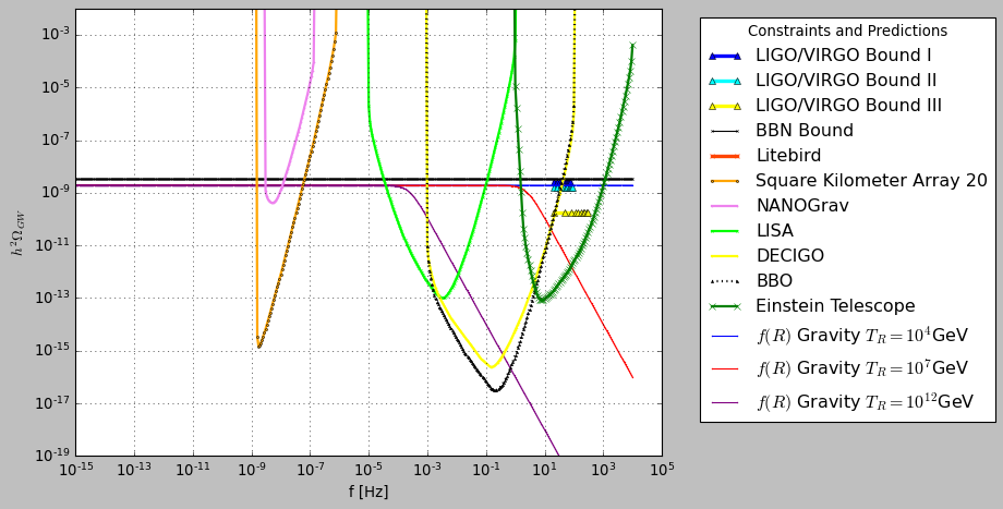
Figure 1: The $h^{2}$-scaled gravitational wave energy spectrum for a geometrically realized constant EoS $w$-era by $f(R)$ gravity for the reheating temperature being $T_{R}=10^{12}$GeV (purple), $T_{R}=10^{7}$GeV (red) and to (blue) $T_{R}=10^{4}$GeV.

The first integral in Eq. (15) is negligible, but the second integration yields, $\int_{z_{pr}}^{z_{end}}\frac{a_{M_{2}}}{1+z^{\prime}}{\rm dz^{\prime}}\sim-24$. Therefore, the overall amplification factor is of the order $e^{-2\mathcal{D}}\sim\mathcal{O}(10^{10})$, and in Fig. 1 we plot the $h$-scaled energy spectrum of the primordial gravitational waves for three distinct reheating temperatures, namely a high $T_{R}=10^{12}$GeV (purple), an intermediate reheating temperature $T_{R}=10^{7}$GeV (red) and a low reheating temperature $T_{R}=10^{4}$GeV (blue). Apparently for the current model, the results presented in Fig. 1 indicate firstly that the predicted gravitational wave signal is compatible with the NANOGrav observation [16] since it is detectable and only the purple curve which corresponds to the highest reheating temperature is excluded because it violates the LIGO-Virgo constraints. Also we need to note that in the context of the present model, there is no need to have a significantly low reheating temperature, which is a mentionable feature indicating that the reheating temperature requirement for explaining the NANOGrav results is model dependent. We need now to discuss the fundamental features of this kind of signals. Firstly it is quite characteristic since it is quite flat. Thus, this is a characteristic $f(R)$ gravity spectrum, which is the same as the single field inflation spectrum, which are flat, but enhanced by a significant factor, however it still remains quite flat. Also it is noticeable that the signal can also be detected by the LISA and the Einstein Telescope in the future. This is the first characteristic signal which can be obtained by a specific class of theories, like an $f(R)$ gravity.

III Peaks in the Primordial Waves Energy Spectrum I: Einstein-Gauss-Bonnet Theories

Another class of possible observations in the current and future gravitational waves interferometers is related with peaks in the energy spectrum of primordial gravitational waves. We shall commence with pure Einstein-Gauss-Bonnet theories, which have the characteristic to predict a blue tilted tensor spectral index. These theories are plagued by the unappealing characteristic of predicting a non-trivial gravitational wave speed, different from that of light’s in vacuum. This obstacle can be overcome if the scalar field potential and the Gauss-Bonnet coupling are not free to chose, but they satisfy a specific relation. Such formalism was developed in Refs. [62, 69, 77]. The action for the Einstein-Gauss-Bonnet theory, [62, 69, 77],

$$\centering S=\int{d^{4}x\sqrt{-g}\left(\frac{R}{2\kappa^{2}}-\frac{1}{2}\partial_{\mu}\phi\partial^{\mu}\phi-V(\phi)-\frac{1}{2}\xi(\phi)\mathcal{G}\right)}\,,\@add@centering$$ (16)

with $R$ denoting the Ricci scalar, $\kappa=\frac{1}{M_{p}}$ with $M_{p}$ being the reduced Planck mass and also $\mathcal{G}$ denotes the Gauss-Bonnet invariant which is explicitly $\mathcal{G}=R^{2}-4R_{\alpha\beta}R^{\alpha\beta}+R_{\alpha\beta\gamma\delta}R^{\alpha\beta\gamma\delta}$ with $R_{\alpha\beta}$ and $R_{\alpha\beta\gamma\delta}$ denoting the Ricci and Riemann tensors respectively.

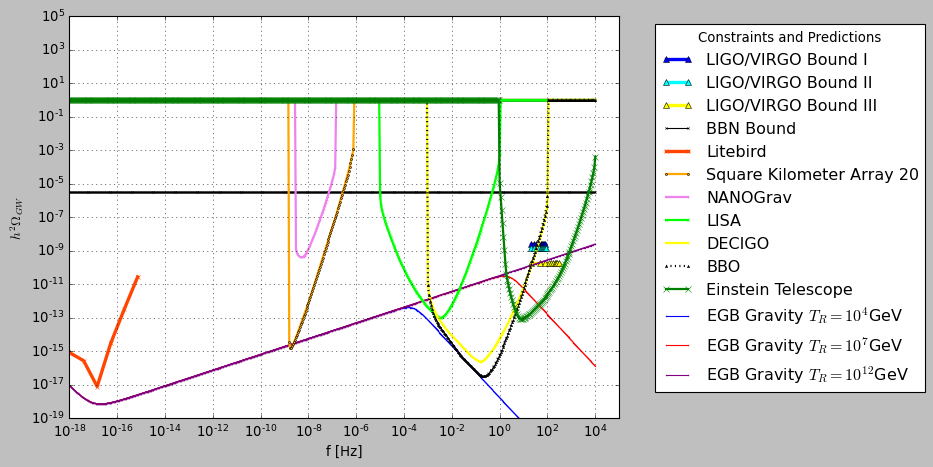
Figure 2: The $h^{2}$-scaled gravitational wave energy spectrum for Einstein-Gauss-Bonnet theory vs the sensitivity curves of future gravitational waves experiments for three reheating temperatures, with a blue tensor spectral index $n_{\mathcal{T}}\sim 0.37$.

Following Refs. [62, 69, 77], if the gravitational wave speed is demanded to be equal to unity in natural units, and thus equal to that of light’s, the slow-roll indices take the following form [69],

$$\centering\epsilon_{1}\simeq\frac{\kappa^{2}}{2}\left(\frac{\xi^{\prime}}{\xi^{\prime\prime}}\right)^{2}\,,\@add@centering$$ (17)

$$\centering\epsilon_{2}\simeq 1-\epsilon_{1}-\frac{\xi^{\prime}\xi^{\prime\prime\prime}}{\xi^{\prime\prime 2}}\,,\@add@centering$$ (18)

$$\centering\epsilon_{3}=0\,,\@add@centering$$ (19)

$$\centering\epsilon_{4}\simeq\frac{\xi^{\prime}}{2\xi^{\prime\prime}}\frac{\mathcal{E}^{\prime}}{\mathcal{E}}\,,\@add@centering$$ (20)

$$\centering\epsilon_{5}\simeq-\frac{\epsilon_{1}}{\lambda}\,,\@add@centering$$ (21)

$$\centering\epsilon_{6}\simeq\epsilon_{5}(1-\epsilon_{1})\,,\@add@centering$$ (22)

with $\mathcal{E}=\mathcal{E}(\phi)$ and $\lambda=\lambda(\phi)$ which are defined in the following way,

$$\mathcal{E}(\phi)=\frac{1}{\kappa^{2}}\left(1+72\frac{\epsilon_{1}^{2}}{\lambda^{2}}\right),\,\,\,\lambda(\phi)=\frac{3}{4\xi^{\prime\prime}\kappa^{2}V}\,.$$ (23)

The inflationary observational indices are defined as follows,

$$\centering n_{\mathcal{S}}=1-4\epsilon_{1}-2\epsilon_{2}-2\epsilon_{4}\,,\@add@centering$$ (24)

$$n_{\mathcal{T}}=-2\left(\epsilon_{1}+\epsilon_{6}\right)\,,$$ (25)

$$r=16\left|\left(\frac{\kappa^{2}Q_{e}}{4H}-\epsilon_{1}\right)\frac{2c_{A}^{3}}{2+\kappa^{2}Q_{b}}\right|\,,$$ (26)

with $c_{A}$ being the sound speed,

$$\centering c_{A}^{2}=1+\frac{Q_{a}Q_{e}}{3Q_{a}^{2}+\dot{\phi}^{2}(\frac{2}{\kappa^{2}}+Q_{b})}\,,\@add@centering$$ (27)

and also with,

$$Q_{a}=-4\dot{\xi}H^{2},\,\,\,Q_{b}=-8\dot{\xi}H,\,\,\,Q_{t}=F+\frac{Q_{b}}{2},$$ (28)

$$Q_{c}=0,\,\,\,Q_{e}=-16\dot{\xi}\dot{H}\,.$$

Using the above, the observational indices of inflation can be significantly simplified in the following way,

$$r\simeq 16\epsilon_{1}\,,$$ (29)

$$n_{\mathcal{T}}\simeq-2\epsilon_{1}\left(1-\frac{1}{\lambda}+\frac{\epsilon_{1}}{\lambda}\right)\,.$$ (30)

There are various Einstein-Gauss-Bonnet models in the recent literature [69] which can be compatible with the GW170817 event while at the same time provide a viable phenomenology with a blue tilted tensor spectral index. Without getting into a detailed analysis of some model here, we shall consider the model,

$$\xi(\phi)=\beta\exp\left(\left(\frac{\phi}{M}\right)^{2}\right)\,,$$ (31)

where $\beta$ is a dimensionless parameter, and also $M$ is a free parameter with mass dimensions $[m]^{1}$. In the formalism of Ref. [69], the scalar potential and the Gauss-Bonnet coupling are constrained via a non-trivial differential equation, so for the case at hand the scalar potential is found to be,

$$\centering V(\phi)=\frac{3}{3\gamma\kappa^{4}+4\beta\kappa^{4}e^{\frac{\phi^{2}}{M^{2}}}}\,,\@add@centering$$ (32)

where $\gamma$ is a dimensionless integration constant. It should be noted that for large field values, decays quite fast, but note here that the slow-roll conditions are not realized and controlled solely from the scalar potential, but also for the non-minimal Gauss-Bonnet coupling function $\xi(\phi)$. For this model, the slow-roll indices become,

$$\centering\epsilon_{1}\simeq\frac{\kappa^{2}M^{4}\phi^{2}}{2\left(M^{2}+2\phi^{2}\right)^{2}}\,,\@add@centering$$ (33)

$$\centering\epsilon_{2}\simeq\frac{M^{4}\left(2-\kappa^{2}\phi^{2}\right)-4M^{2}\phi^{2}}{2\left(M^{2}+2\phi^{2}\right)^{2}}\,,\@add@centering$$ (34)

$$\centering\epsilon_{3}=0\,,\@add@centering$$ (35)

$$\centering\epsilon_{5}\simeq-\frac{4\beta\phi^{2}e^{\frac{\phi^{2}}{M^{2}}}}{\left(M^{2}+2\phi^{2}\right)\left(3\gamma+4\beta e^{\frac{\phi^{2}}{M^{2}}}\right)}\,,\@add@centering$$ (36)

$$\centering\epsilon_{6}\simeq-\frac{2\beta\phi^{2}e^{\frac{\phi^{2}}{M^{2}}}\left(M^{4}\left(2-\kappa^{2}\phi^{2}\right)+8M^{2}\phi^{2}+8\phi^{4}\right)}{\left(M^{2}+2\phi^{2}\right)^{3}\left(3\gamma+4\beta e^{\frac{\phi^{2}}{M^{2}}}\right)}\,,\@add@centering$$ (37)

and the observational indices of inflation are,

$$n_{\mathcal{S}}\simeq-1-\frac{\kappa^{2}M^{4}\phi^{2}}{\left(M^{2}+2\phi^{2}\right)^{2}}+\frac{4\phi^{2}\left(3M^{2}+2\phi^{2}\right)}{\left(M^{2}+2\phi^{2}\right)^{2}}$$ (38)

$$+\frac{4608\beta^{2}\phi^{6}e^{\frac{2\phi^{2}}{M^{2}}}\left(6\gamma\phi^{2}+16\beta e^{\frac{\phi^{2}}{M^{2}}}\left(M^{2}+\phi^{2}\right)+9\gamma M^{2}\right)}{\left(M^{2}+2\phi^{2}\right)^{4}\left(3\gamma+4\beta e^{\frac{\phi^{2}}{M^{2}}}\right)^{3}}\,,$$

regarding the spectral index of scalar perturbations, while spectral index of tensor perturbations reads,

$$n_{\mathcal{T}}\simeq\frac{\phi^{2}\left(-4\beta e^{\frac{\phi^{2}}{M^{2}}}\left(M^{4}\left(3\kappa^{2}\phi^{2}-2\right)+\kappa^{2}M^{6}-8M^{2}\phi^{2}-8\phi^{4}\right)-3\gamma\kappa^{2}M^{4}\left(M^{2}+2\phi^{2}\right)\right)}{\left(M^{2}+2\phi^{2}\right)^{3}\left(3\gamma+4\beta e^{\frac{\phi^{2}}{M^{2}}}\right)}\,.$$ (39)

and finally, the tensor-to-scalar ratio takes the form,

$$r\simeq\frac{8\kappa^{2}M^{4}\phi^{2}}{\left(M^{2}+2\phi^{2}\right)^{2}}\,.$$ (40)

which yields a tensor spectral index values of the order $n_{\mathcal{T}}=[0.378856,0.379088]$ and a tensor-to-scalar ratio $r\sim 0.003$, for $\mu=[22.09147657871,22.09147657877]$, $\beta=-1.5$, $\gamma=2$, for $N=60$ $e$-foldings. Also we assume three reheating temperatures, like in the $f(R)$ gravity case, namely a high reheating temperature $T_{R}=10^{12}$GeV, an intermediate reheating $T_{R}=10^{7}$GeV and a low reheating temperature $T_{R}=10^{4}$GeV. In Fig. 2 we plot the $h^{2}-$scaled energy spectrum of the primordial gravitational waves for the above Einstein-Gauss-Bonnet model with $n_{\mathcal{T}}\sim 0.37$ for the three distinct reheating temperatures. As it can be seen, the spectrum has a characteristic peak-like form, with the peak being affected by the reheating temperature and by the tensor spectral index. Also in Fig. 3 we plot the $h^{2}$-scaled energy spectrum of the primordial gravitational waves for $n_{\mathcal{T}}\sim 0.97$ (purple curve) and $n_{\mathcal{T}}=1.1$ (blue and red curves).

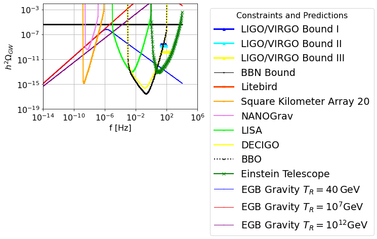
Figure 3: The $h^{2}$-scaled gravitational wave energy spectrum for Einstein-Gauss-Bonnet theory vs the sensitivity curves of future gravitational waves experiments for three reheating temperatures, with a blue tensor spectral index $n_{\mathcal{T}}\sim 0.97$.

From both Figs. 2 and 3 we can see that a single Einstein-Gauss-Bonnet gravity yields a peak-like signal and in order for the signal to be detected by the NANOGrav experiment, it is required that the tensor spectral index must be quite large of the order $n_{\mathcal{T}}=1.1$ and the reheating temperature must be quite low of the order $\mathcal{O}(40)\,$GeV, see the blue curve in Fig. 3. For higher reheating temperatures and for $n_{\mathcal{T}}=1.1$, the signal violates the BBN bound, see the red curve in Fig. 3.

In conclusion, Einstein-Gauss-Bonnet theories yield a peak-like gravitational wave energy spectrum, which can be compatible with the NANOGrav result if the tensor spectral index is of the order unity and the reheating temperature is of the GeV order. This result is compatible with the findings of Ref. [27] which also requires a low-reheating temperature and a large blue tilted tensor spectrum. However, a low-reheating temperature puts in peril theories which predict primordial gravitational waves via the electroweak phase transitions. Specifically the first order electroweak phase transition requires a reheating temperature of the order of $100\,$GeV, so if the NANOGrav result is correct, a low reheating temperature can put the electroweak phase transition theory into peril. This reheating temperature issue however proves to be model dependent as we show in the next section.

IV Peaks in the Primordial Waves Energy Spectrum II: Axion-Higgs Higher Order Interactions with a Blue Tilted Tensor Spectral Index

Another class of models that may yield a peak-like energy spectrum of primordial gravitational waves involves higher order non-renormalizable couplings between the axion and the Higgs particle [78]. The axion is one among several currently considered dark matter candidates, for a mainstream of research and review articles on the axion see [79, 80, 81, 82, 83, 84, 85, 86, 87, 88, 89, 90, 91, 92, 93, 94, 95, 96, 97]. It is also mentionable that in the future, experiments will probe extremely small axion masses in the range $10^{-8}-10^{-16}\,$eV [98]. In general, couplings between the Higgs and the axion are quite frequently used in the literature [99, 100, 101], but recently higher order non-renormalizable couplings were considered [78]. These higher order non-renormalizable terms belong to an effective theory that is active at a scale $M$ which is higher than the electroweak scale. Once the electroweak breaking occurs during the reheating era, when the temperature was of the order $T\sim 100\,$GeV, the effective operators directly modify the axion potential, causing new interesting physics in the axion sector which may have a direct effect on the primordial gravitational waves energy spectrum, see [78] for details. In this paper we shall present in brief the mechanism described in Ref. [78], we shall show that the energy spectrum of the primordial gravitational waves has a peak-like form and we shall investigate the conditions needed in order for the energy spectrum to be detectable from the NANOGrav collaboration. The result is quite interesting as we now discuss in brief. Once the electroweak breaking occurs, the axion potential acquires a new minimum and the axion oscillations around the origin are destabilized. The axion is free to move along the potential to reach the new minimum. This can be done in a quick way, in which case the total EoS during the reheating era is disturbed and it takes values larger than $w=1/3$, so it is similar to a short kination era only in the axion dynamics [102, 103, 104, 105, 106, 107, 108]. However, this roll down to the axion new minimum can occur in a slow-roll way, thus the total EoS during the reheating era is smaller than $w=1/3$. It is actually this scenario that may yield a detectable primordial gravitational wave energy spectrum, if accompanied by a reheating temperature of the order $T\sim 400\,$GeV. Regardless of the way that the axion approaches its new minimum, once it reaches it, the new vacuum instantly decays to the Higgs vacuum which is energetically more favorable in the Universe. We assume that the axion dynamics is described by the misalignment axion scenario [82, 84], in which case the primordial Peccei-Quinn $U(1)$ symmetry is broken during inflation and the axion is the radial component of the primordial complex scalar field that has the $U(1)$ Peccei-Quinn symmetry. During the inflationary era, the axion has a large misaligned value, of the order $\phi_{i}\sim f_{a}$, with $f_{a}$ being the axion decay constant, which is larger than $f_{a}>10^{9}\,$GeV. In the misalignment scenario, the axion potential is primordially,

$$V_{a}(\phi)=m_{a}^{2}f_{a}^{2}\left(1-\cos\left(\frac{\phi}{f_{a}}\right)\right)\,,$$ (41)

hence during inflation and thereafter we have $\phi/f_{a}<1$, so the potential is approximately equal to,

$$V_{a}(\phi)\simeq\frac{1}{2}m_{a}^{2}\phi^{2}\,.$$ (42)

Once the axion mass becomes of the same order as the Hubble rate, the axion reaches the minimum of its potential and commences oscillations around the origin, and redshifts as cold dark matter.

In the present model we shall assume that the axion couples to the Higgs sector via higher order non-renormalizable operators as follows,

$$V(\phi,h)=V_{a}(\phi)-m_{H}^{2}|H|^{2}+\lambda_{H}|H|^{4}-\lambda\frac{|H|^{2}\phi^{4}}{M^{2}}+g\frac{|H|^{2}\phi^{6}}{M^{4}}\,,$$ (43)

where $V_{a}(\phi)$ is defined in Eq. (41), and the Higgs field before the electroweak symmetry breaking is $H=\frac{h+ih_{1}}{\sqrt{2}}$, with the Higgs mass being $m_{H}=125$ GeV [109] and $\lambda_{H}$ stands for the Higgs self-coupling $\frac{v}{\sqrt{2}}=\left(\frac{-m_{H}^{2}}{\lambda_{H}}\right)^{\frac{1}{2}}$, with $v$ being the electroweak symmetry breaking scale $v\simeq 246\,$GeV. The axion mass shall be assumed to be of the order $m_{a}\sim 10^{-10}\,$eV and the effective non-renormalizable operators are assumed to originate from an effective theory with energy scale of the order $M=20-100\,$TeV These six and eight dimensional operators are motivated by the lack of any new particle detection in the LHC in the energy range $125\,$GeV-15 TeV center of mass. The Wilson coefficients will be assumed to be $\lambda\sim\mathcal{O}(10^{-20})$ and $g\sim\mathcal{O}(10^{-5})$. Also, we shall assume that the electroweak phase transition actually occurs at $T\sim 100\,$GeV, and it is first order [110, 111, 112, 113, 114, 115, 116, 117, 118, 119, 120, 113, 121, 122, 123, 124, 125, 126, 114, 127, 123, 128, 129, 130]. After the electroweak phase transition occurs, the Higgs acquires a vacuum expectation value $H=v+\frac{h+ih_{1}}{\sqrt{2}}$, and thus at leading order, the tree order axion potential is modified and takes the following form,

$$\mathcal{V}_{a}(\phi)=V_{a}(\phi)-\lambda\frac{v^{2}\phi^{4}}{M^{2}}+g\frac{v^{2}\phi^{6}}{M^{6}}\,,$$ (44)

where $V_{a}(\phi)$ is defined in Eq. (41). In order to have a concrete idea on the deformation of the axion potential, after the electroweak symmetry breaking, assume that $m_{a}\sim 10^{-10}$eV, $M=20\,$TeV and the Wilson coefficients are $\lambda\sim\mathcal{O}(10^{-20})$ and $g\sim\mathcal{O}(10^{-5})$, and we plot the new axion potential in Fig. 4 (left plot) and the Higgs effective potential (right plot). Notice that the Higgs minimum $(h,\phi)=(v,0)$ is energetically more favorable than the axion potential minimum $(h,\phi)=(0,v_{s})$.

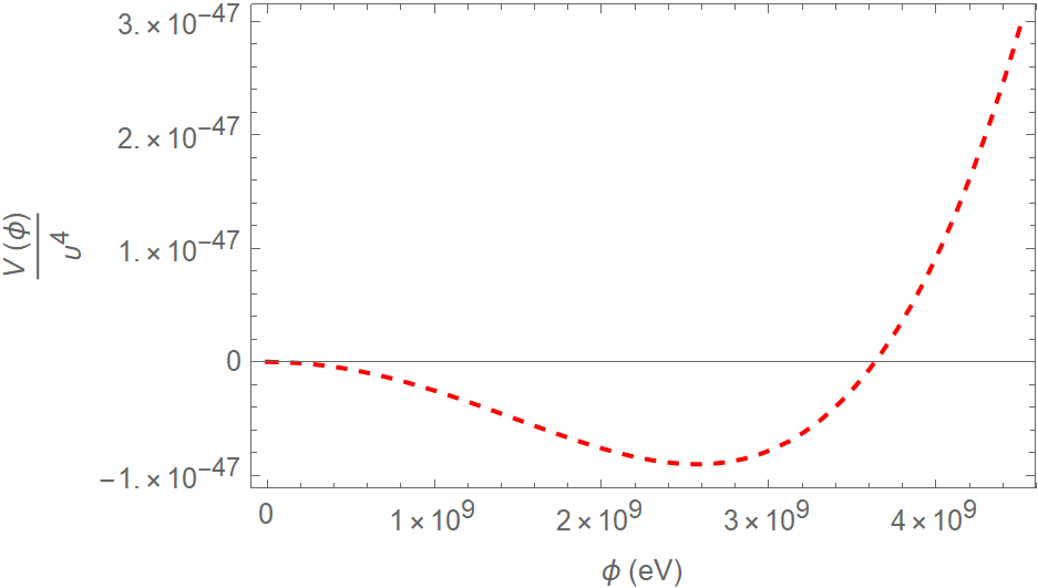
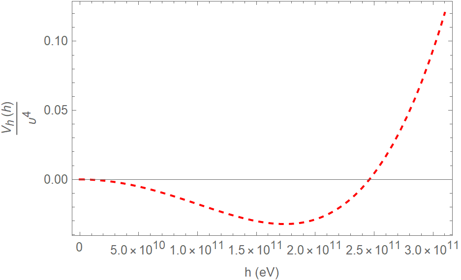
Figure 4: The modified axion effective potential for $m_{a}\sim 10^{-10}$eV, and the effective theory parameters being $M=20\,$TeV and $\lambda\sim\mathcal{O}(10^{-20})$ and $g\sim\mathcal{O}(10^{-5})$ (left plot). Also the Higgs potential after the electroweak symmetry breaking is depicted in the right plot.

This said behavior for the axion potential after the electroweak breaking also holds true even if the one-loop corrections are added in the axionic sector,

$$V^{1-loop}(\phi)=\frac{m_{eff}^{4}(\phi)}{64\pi^{2}}\left(\ln\left(\frac{m_{eff}^{2}(\phi)}{\mu^{2}}\right)-\frac{3}{2}\right)\,,$$ (45)

with $m_{eff}^{2}(\phi)$,

$$m_{eff}^{2}(\phi)=\frac{\partial^{2}V(\phi,h)}{\partial\phi^{2}}=m_{a}^{2}-\frac{6\lambda v^{2}\phi^{2}}{M^{2}}+\frac{15gv^{2}\phi^{4}}{M^{4}}\,,$$ (46)

and $\mu$ stands for the renormalization scale. Now since two different vacua occur in the theory, one the axion new minimum and the competing Higgs vacuum, the dominant vacuum will be determined by the depths of the competing vacua, and in our case we have,

$$V_{h}(h)=(v)\gg V(\phi)=(v_{s})\,,$$ (47)

thus once the axion reaches its minimum, the new vacuum decays instantly in the Higgs vacuum. A detailed analysis on this can be found in Ref. [78]. The instant decay of the axion scalar field newly developed new vacuum state is unavoidable since the axion vacuum is competing with the Higgs vacuum state, thus the Higgs vacuum is energetically more favorable and therefore the axion vacuum instantly decays to the Higgs vacuum. A pictorial representation of this procedure can be seen in Fig. 5.

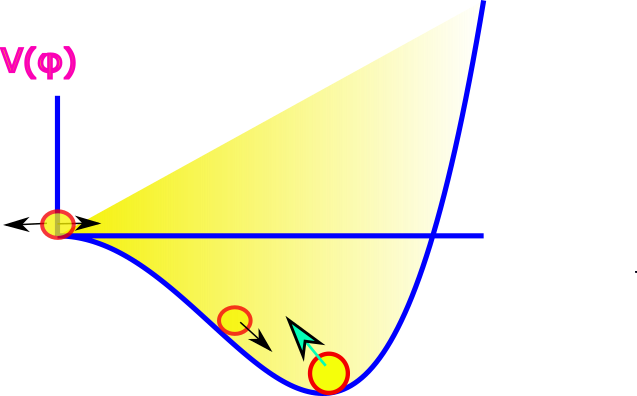
Figure 5: The axion scalar potential $V(\phi)$ in the post-electroweak symmetry breaking epoch develops a deeper minimum at the direction $(\phi)=(v_{s})$. This new minimum disrupts the axion oscillations at the origin and the axion is free to move toward to its minimum, either in a slow-roll way or following a kination trajectory. Once the axion reaches its new minimum, the new axion scalar minimum in the Universe is not energetically preferable compared to the Higgs minimum $(h)=(v)$, thus the axion minimum decays to the Higgs minimum and the potential energy of the decay is transferred to axion kinetic energy, which makes the axion to oscillate around the origin in an unbounded way. The oscillations become destabilized after some time and the same procedure is repeated perpetually.

Now let us discuss the way that the axion reaches the its new vacuum. Before the electroweak breaking, the axion behaved as cold dark matter and it oscillated around the minimum of its potential. However, in the post-electroweak breaking epoch, the axion potential develops a new minimum and thus the axion is destabilized. The oscillations are disrupted and the axion is free to move along the trajectory in the field space, that leads to the new minimum. There are two ways for the axion evolution once the axion oscillations are disrupted, the first is to swiftly evolve to its new minimum, and the second is to evolve in a slow-roll way. These two distinct evolutions which have different kinetic energy for the axion, affect in a different way the total background EoS of the Universe, which gets disturbed from the radiation domination value $w=1/3$. In fact, if the axion evolves swiftly to its new minimum, its kinetic energy dominates over its potential energy and the axion EoS is described by a stiff EoS $w_{a}\simeq 1$, thus the total EoS of the Universe $w$ becomes larger than the radiation domination value $w=1/3$. This possibility was examined in Ref. [78] but by our analysis performed in this paper, it seems that the NANOGrav result can be explained only if the axion actually slow-rolls to its new minimum and the total EoS of the Universe is actually smaller than the radiation domination value $w=1/3$. So in this paper we shall study the second scenario, in which the axion slow-rolls down to its new minimum. Its EoS is thus $w_{a}\sim-1$, thus this could perceived as an early dark energy era caused by the axion and this might significantly affect the total EoS of the Universe during the radiation domination era. For the purposes of this paper we shall be more moderate and we shall assume that the axion slow-roll era affects the total EoS of the Universe in a minimal way and it changes it from the radiation domination value $w=1/3$ to $w=0.28$. As we shall see, this plays an important role for the explanation of the detected gravitational wave signal from the NANOGrav collaboration.

The destabilization of the axion during the reheating era can have observable effects on the energy spectrum of the primordial gravitational waves via the modes that re-enter the Hubble horizon at exactly the era at which the axion slow-rolls to its new minimum. For the purposes of this paper, we shall assume that the axion slow-roll and decay process occurs two and four times during the radiation domination era, and at two and four distinct frequencies. Also we shall assume three different reheating temperatures, a high reheating temperature $T_{R}=10^{12}\,$GeV, an intermediate $T_{R}=10^{7}\,$GeV and a low reheating temperature $T_{R}=400\,$GeV. The modes that reenter the horizon at a reheating temperature of the order $T_{R}=10^{7}\,$GeV have a wavenumber of the order $k_{R}=1.19\times 10^{15}$Mpc^-1. Therefore, for modes that reentered the horizon during the era which NANOGrav probes, should have wavenumbers larger than $k_{t_{1}}=15\times 10^{5}$Mpc^-1. So we shall assume that the axion slow-roll and decay process occurs firstly at two frequencies and specifically at $k_{t_{1}}=15\times 10^{5}$Mpc^-1 , $k_{t_{2}}=10\times 10^{9}$Mpc^-1 and secondly at four distinct frequencies at $k_{t_{1}}=15\times 10^{5}$Mpc^-1, $k_{t_{2}}=6.5\times 10^{9}$Mpc^-1, $k_{t_{3}}=10\times 10^{9}$Mpc^-1 and $k_{t_{4}}=15\times 10^{9}$Mpc^-1. We shall explore the effect of these decays on the energy spectrum of the primordial gravitational waves. As we will show, in order for the NANOGrav result to be explained, one needs a low reheating temperature of the order $T_{R}\sim 400\,$GeV, and a blue tilted tensor spectrum coming from inflation of the order $n_{\mathcal{T}}=0.97$ if the tensor-to-scalar ratio is of the order $\sim\mathcal{O}(10^{-3})$. However, if the tensor-to-scalar ratio is assumed to be larger, the tensor spectral index can be smaller, and specifically larger than $n_{\mathcal{T}}=0.55$. Such a blue tilt can come from an Einstein-Gauss-Bonnet theory or some other inflationary or more exotic scenario. This kind of behavior was also stressed in the recent work [27], but in our case the required tensor spectral index is smaller and the reheating temperature can be 10 times larger than the one used in Ref. [27].

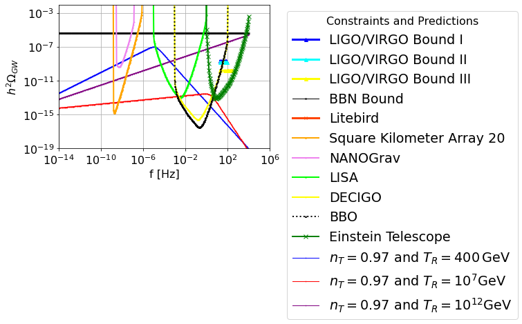
Figure 6: The $h^{2}$-scaled gravitational wave energy spectrum for and inflationary theory with a blue tensor spectral index, with three distinct reheating temperatures, for two axion vacuum decays. The NANOGrav result is verified in the case of a low reheating temperature of the order $T\sim 400\,$GeV. We assumed a preceding inflationary era with $n_{\mathcal{T}}=0.97$ and $r\sim\mathcal{O}(10^{-3})$.

Now, if during the radiation domination era the axion slow-rolls its potential and the new vacuum decays at some wavenumber $k_{\mu}$, and if the background EoS is changed from the radiation domination value $w=1/3$ to some $w$, then the $h^{2}$-scaled energy spectrum of the primordial gravitational waves changes by the following multiplication factor, $\sim\left(\frac{k}{k_{\mu}}\right)^{r_{c}}$, with $r_{c}=-2\left(\frac{1-3w}{1+3w}\right)$ [131]. For the purposes of this paper we shall assume that the total EoS parameter is changed from the $w=1/3$ value to $w=0.28$ two or four distinct times during the radiation domination era, thus, the $h^{2}$-scaled energy spectrum is changed as follows,

$$\Omega_{\rm gw}(f)=S_{k}(f)\times\frac{k^{2}}{12H_{0}^{2}}r\mathcal{P}_{\zeta}(k_{ref})\left(\frac{k}{k_{ref}}\right)^{n_{T}}\left(\frac{\Omega_{m}}{\Omega_{\Lambda}}\right)^{2}\left(\frac{g_{*}(T_{\rm in})}{g_{*0}}\right)\left(\frac{g_{*s0}}{g_{*s}(T_{\rm in})}\right)^{4/3}\left(\overline{\frac{3j_{1}(k\tau_{0})}{k\tau_{0}}}\right)^{2}T_{1}^{2}\left(x_{\rm eq}\right)T_{2}^{2}\left(x_{R}\right)\,,$$

with the multiplication factor $S_{k}(f)$ being,

$$S_{k}(f)=\left(\frac{k}{k_{t_{1}}}\right)^{r_{c}}\times\left(\frac{k}{k_{t_{2}}}\right)^{r_{c}}\,,$$ (48)

for two distinct axion slow-roll and decays, while for four distinct decays the multiplication factor becomes,

$$S_{k}(f)=\left(\frac{k}{k_{t_{1}}}\right)^{r_{c}}\times\left(\frac{k}{k_{t_{2}}}\right)^{r_{c}}\times\left(\frac{k}{k_{t_{3}}}\right)^{r_{c}}\times\left(\frac{k}{k_{t_{4}}}\right)^{r_{c}}\,.$$ (49)

In Figs. 6 and 7 we have plotted the $h^{2}$-scaled energy spectrum of the primordial gravitational waves with two and four axion decays respectively, for various reheating temperatures and a blue tilted tensor spectrum with $n_{\mathcal{T}}=0.97$ and a tensor-to-scalar ratio of the order $r\sim 0.003$. As it can be seen in both plots, the energy spectrum of the primordial gravitational waves has a peak-like form in characteristic frequencies. Regarding the NANOGrav observation, in order for this axion-Higgs scenario to produce a detectable gravitational wave signal, it is required that the tensor-spectral index is blue tilted of the order $n_{\mathcal{T}}=0.97$ or larger, a low reheating temperature of the order $T_{R}\sim 400\,$GeV and two or higher axion slow-roll evolution and decays during the radiation domination era. Actually, for the case that four decays take place, the signal is more pronounced, see for example Fig. 7.

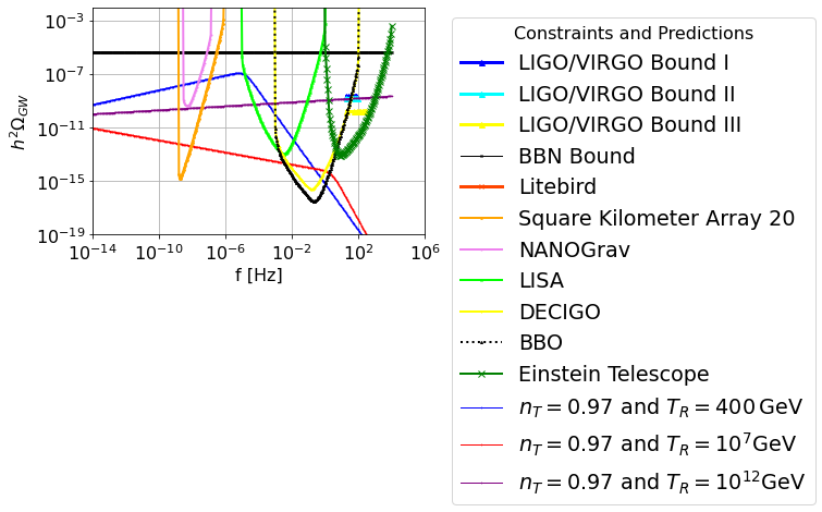
Figure 7: The $h^{2}$-scaled gravitational wave energy spectrum for and inflationary theory with a blue tensor spectral index, with three distinct reheating temperatures, for four axion vacuum decays. The NANOGrav result is verified in the case of a low reheating temperature of the order $T\sim 400\,$GeV.

It is mentionable that in both cases in which the signal is detectable by the NANOGrav collaboration, it is also detectable by LISA but not from the Einstein Telescope. In conclusion, in the Higgs-axion model we analyzed in this section, the energy spectrum of the primordial gravitational waves has a peak-like form at a specific frequency which depends on when and how many times the axion slow-rolls its potential and its vacuum decays to the Higgs vacuum. Moreover, the recent NANOGrav result can be explained if the inflationary era produces a blue tilted tensor spectral index, larger than $n_{\mathcal{T}}\geq 0.9$ and if the reheating temperature is low enough of the order $T_{R}\sim 400\,$GeV. Qualitatively similar conclusions regarding the blue tilted tensor spectrum and the low reheating temperature were reported in Ref. [27], regarding the NANOGrav result. However in our case, the reheating temperature is low, but not as low as in Ref. [27]. In our case, the lowest reheating temperature that is needed in order to explain the NANOGrav result is four times larger than the electroweak symmetry breaking temperature.

V Conclusions and Discussion

In this article we presented the various distinct forms of the energy spectrum of the primordial gravitational waves using several characteristic theories. We showed that the energy spectrum can either be flat or it can have a peak-like form. We used three typical theories that can produce such kind of spectrums, $f(R)$ gravity, Einstein-Gauss-Bonnet gravity and finally an inflationary theory with a blue spectrum with abnormal reheating era caused by axion-Higgs higher order couplings. As we showed for the case of $f(R)$ gravity, the signal can only be observed if an abnormal reheating era is generated by geometric $f(R)$ gravity terms. In this case the spectrum is flat and also can be detected by all the future gravitational wave experiments, including the current NANOGrav experiment. Regarding the Einstein-Gauss-Bonnet theory, only a theory with a blue tilted tensor spectral index of the order $n_{\mathcal{T}}\sim\mathcal{O}(1)$ and a low reheating temperature of the order $T_{R}\sim\mathcal{O}(40)\,$GeV can be compatible with the NANOGrav result and also compatible with the BBN bounds. In all the cases, the Einstein-Gauss-Bonnet class of modified gravity theories produce a peak-like energy spectrum. Accordingly we examined another class of theories which leads to an observable energy spectrum of primordial gravitational waves. This theory contains higher order non-renormalizable couplings between the Higgs and the axion and in effect the radiation domination era is disrupted by short early dark energy axion eras. In order for the signal to be detected by the NANOGrav experiment, it is important to have a blue tilted tensor inflationary spectrum and also to have two to four axion slow-roll eras.

In conclusion, in order for these theories to describe successfully the NANOGrav signal one must have either one of the following:

• An abnormal reheating era geometrically realized by an $f(R)$ gravity.

• An abnormal reheating era combined with a relatively low reheating temperature $T_{R}\sim 400\,$GeV and a blue tilted tensor spectral index $n_{\mathcal{T}}\geq 0.97$.

• A sufficiently low reheating temperature of the order $T_{R}\sim 40\,$GeV and a sufficiently blue tensor spectral index $n_{\mathcal{T}}\geq 1.1$, regarding Einstein-Gauss-Bonnet theories of gravity. This is highly non-trivial to achieve though in the context of Einstein-Gauss-Bonnet gravity as it can be shown.

Thus in most of the cases, the low reheating temperature, the blue tilted tensor spectrum and an abnormal reheating era seem to be the factors that determine whether the model can produce the NANOGrav signal. The next steps after the astonishing NANOGrav detection of the first stochastic signal is the commence of the other two well anticipated experiments, LISA and Einstein Telescope. Only the joint observations of a stochastic signal may shed some light on which theory describes the detected stochastic gravitational wave signal. Also the joint signal can also give hints on the reheating temperature itself and may also determine whether the electroweak phase transition ever occurred. Indeed, if it proven that the reheating temperature never reached 100 GeV, then this feature would put the theory of electroweak phase transition in peril, and an alternative mechanism, distinct from a thermal phase transition, will be needed to explain the electroweak symmetry breaking.

Finally, it is worth commenting on the cosmological perspective of the NANOGrav signal. It seems that the spectral slope of the 2023 NANOGrav signal is 3$\sigma$ off the astrophysical prediction coming from supermassive black holes mergers [27]. This feature was also reluctantly discussed in [132], based on the 2020 NANOGrav article. Although specific astrophysical models can be marginally compatible with the NANOGrav 2023 result [134], for the moment there are too many arguments to be explained for the astrophysical perspective. Specifically, the complete absence of anisotropies [133], the incomplete theoretical solution to the final parsec problem [134] which is a theoretical riddle to date, the absence of single supermassive black hole binaries merger events in the NANOGrav 2023 announcements, makes us think that from the Occam’s razor perspective, the cosmological perspective of the 2023 signal is more likely, compared to the astrophysical perspective. This argument is statistically supported currently by the fact that the many cosmological models are found to provide a better fit to the NANOGrav 2023 stochastic gravitational wave background than the astrophysical sources, a better fit which in Bayes factors ranges from 10 to 100 [135]. However, it is rather too early to make conclusions on the source of the stochastic gravitational wave background. Surely though, a decisive conclusion can be made once the spatial anisotropies are measured, see Ref. [136] for a recent study on this. As expected, this bright new observation has attracted a lot of attention for new physics explanations [137, 138, 139, 140, 141, 142, 143, 144, 145, 146, 147, 148, 149, 150, 151, 152, 153, 154, 155], see also [72, 156, 157, 158, 159, 160, 161] for older works which pointed out the ability of NANOGrav to detect a stochastic gravitational wave signal coming from various sources. Also it is notable that the stochastic signal detected may be explained by axion physics too [139, 140], see also [97] for preceding works.

Lastly, let us further specify the cosmologically viable theories that can describe the NANOGrav signal. It seems that conventional theories like Einstein-Gauss-Bonnet gravity requires a large blue-tilted tensor-spectral index, which is hard to achieve in the slow-roll approximation. In fact, other theories that also yield blue-tilted tensor spectral index like string-gas theories [162, 163, 164], do not yield such a large tensor spectral index, without violating the Planck 2018 constraints. In fact, the only theory of inflation which can be potentially compatible with the 2023 NANOGrav signal is the non-local version of the Starobinsky model [165, 166, 167], which also yields non-Gaussianities of the order unity. Thus although most theories that yield blue tensor spectral index are incapable to describe the NANOGrav signal, the non-local version of the Starobinsky model can provide a significantly large blue tilted, thus combined with the Higgs-axion model can in principle explain the NANOGrav 2023 signal. Also the $f(R)$ gravity realized abnormal reheating era can also explain the NANOGrav signal, but this is not the end of the story for sure. One cannot be conclusive at this point for any solution give, phase transition, cosmic strings or some combinations of inflation with the models and scenarios we presented in this paper. NANOGrav 2023 was the start of a new era for physics, the era of the stochastic gravitational wave background. To fully understand it, it is compelling to have available the results from the future experiments like LISA and the Einstein telescope and of course the Square Kilometer Array, combined with more data from NANOGrav. Only then we will be sure, if the signal is astrophysical, cosmological, or a combination of these. Also the shape of the signal across a large frequency range will only give hints for the underlying theory. For example a flat signal appearing in all future experiments, with the same amplitude and energy spectrum will indicate a theory like the model of $f(R)$ gravity with a geometrically realized reheating era we described in a previous section. Or a signal appearing only in the LISA and NANOGrav can point to another direction. For the moment we are excited to be blessed to live in the era that the stochastic background is finally observed and verified. Now a long, exciting and thorny road awaits till we determine the underlying theory that controls the cosmos.

References

- [1] A. D. Linde, Lect. Notes Phys. 738 (2008) 1 [arXiv:0705.0164 [hep-th]].
- [2] D. S. Gorbunov and V. A. Rubakov, “Introduction to the theory of the early universe: Cosmological perturbations and inflationary theory,” Hackensack, USA: World Scientific (2011) 489 p;
- [3] A. Linde, arXiv:1402.0526 [hep-th];
- [4] D. H. Lyth and A. Riotto, Phys. Rept. 314 (1999) 1 [hep-ph/9807278].
- [5] S. Hild, M. Abernathy, F. Acernese, P. Amaro-Seoane, N. Andersson, K. Arun, F. Barone, B. Barr, M. Barsuglia and M. Beker, et al. Class. Quant. Grav. 28 (2011), 094013 doi:10.1088/0264-9381/28/9/094013 [arXiv:1012.0908 [gr-qc]].
- [6] J. Baker, J. Bellovary, P. L. Bender, E. Berti, R. Caldwell, J. Camp, J. W. Conklin, N. Cornish, C. Cutler and R. DeRosa, et al. [arXiv:1907.06482 [astro-ph.IM]].
- [7] T. L. Smith and R. Caldwell, Phys. Rev. D 100 (2019) no.10, 104055 doi:10.1103/PhysRevD.100.104055 [arXiv:1908.00546 [astro-ph.CO]].
- [8] J. Crowder and N. J. Cornish, Phys. Rev. D 72 (2005), 083005 doi:10.1103/PhysRevD.72.083005 [arXiv:gr-qc/0506015 [gr-qc]].
- [9] T. L. Smith and R. Caldwell, Phys. Rev. D 95 (2017) no.4, 044036 doi:10.1103/PhysRevD.95.044036 [arXiv:1609.05901 [gr-qc]].
- [10] N. Seto, S. Kawamura and T. Nakamura, Phys. Rev. Lett. 87 (2001), 221103 doi:10.1103/PhysRevLett.87.221103 [arXiv:astro-ph/0108011 [astro-ph]].
- [11] S. Kawamura, M. Ando, N. Seto, S. Sato, M. Musha, I. Kawano, J. Yokoyama, T. Tanaka, K. Ioka and T. Akutsu, et al. [arXiv:2006.13545 [gr-qc]].
- [12] A. Weltman, P. Bull, S. Camera, K. Kelley, H. Padmanabhan, J. Pritchard, A. Raccanelli, S. Riemer-Sørensen, L. Shao and S. Andrianomena, et al. Publ. Astron. Soc. Austral. 37 (2020), e002 doi:10.1017/pasa.2019.42 [arXiv:1810.02680 [astro-ph.CO]].
- [13] P. Auclair et al. [LISA Cosmology Working Group], [arXiv:2204.05434 [astro-ph.CO]].
- [14] K. N. Abazajian et al. [CMB-S4], [arXiv:1610.02743 [astro-ph.CO]].
- [15] M. H. Abitbol et al. [Simons Observatory], Bull. Am. Astron. Soc. 51 (2019), 147 [arXiv:1907.08284 [astro-ph.IM]].
- [16] G. Agazie et al. [NANOGrav], doi:10.3847/2041-8213/acdac6 [arXiv:2306.16213 [astro-ph.HE]].
- [17] J. Antoniadis, P. Arumugam, S. Arumugam, S. Babak, M. Bagchi, A. S. B. Nielsen, C. G. Bassa, A. Bathula, A. Berthereau and M. Bonetti, et al. [arXiv:2306.16214 [astro-ph.HE]].
- [18] D. J. Reardon, A. Zic, R. M. Shannon, G. B. Hobbs, M. Bailes, V. Di Marco, A. Kapur, A. F. Rogers, E. Thrane and J. Askew, et al. doi:10.3847/2041-8213/acdd02 [arXiv:2306.16215 [astro-ph.HE]].
- [19] H. Xu, S. Chen, Y. Guo, J. Jiang, B. Wang, J. Xu, Z. Xue, R. N. Caballero, J. Yuan and Y. Xu, et al. doi:10.1088/1674-4527/acdfa5 [arXiv:2306.16216 [astro-ph.HE]].
- [20] T. Regimbau, Symmetry 14 (2022) no.2, 270 doi:10.3390/sym14020270
- [21] S. Nojiri, S. D. Odintsov and V. K. Oikonomou, Phys. Rept. 692 (2017) 1 [arXiv:1705.11098 [gr-qc]].
-
[22]
S. Capozziello, M. De Laurentis,
Phys. Rept. 509, 167 (2011);
V. Faraoni and S. Capozziello, Fundam. Theor. Phys. 170 (2010). - [23] S. Nojiri, S.D. Odintsov, eConf C0602061, 06 (2006) [Int. J. Geom. Meth. Mod. Phys. 4, 115 (2007)].
- [24] S. Nojiri, S.D. Odintsov, Phys. Rept. 505, 59 (2011);
- [25] G. J. Olmo, Int. J. Mod. Phys. D 20 (2011) 413 [arXiv:1101.3864 [gr-qc]].
- [26] L. Sebastiani, S. Vagnozzi and R. Myrzakulov, Adv. High Energy Phys. 2017 (2017), 3156915 doi:10.1155/2017/3156915 [arXiv:1612.08661 [gr-qc]].
- [27] Sunny Vagnozzi, [arXiv:2306.16912 [astro-ph.CO]].
- [28] M. Benetti, L. L. Graef and S. Vagnozzi, Phys. Rev. D 105 (2022) no.4, 043520 doi:10.1103/PhysRevD.105.043520 [arXiv:2111.04758 [astro-ph.CO]].
- [29] M. Khlopov and S. R. Chowdhury, Symmetry 15 (2023) no.4, 832 doi:10.3390/sym15040832
- [30] S. Vagnozzi, Mon. Not. Roy. Astron. Soc. 502 (2021) no.1, L11-L15 doi:10.1093/mnrasl/slaa203 [arXiv:2009.13432 [astro-ph.CO]].
- [31] V. K. Oikonomou, Annalen Phys. 534 (2022) no.8, 2200134 doi:10.1002/andp.202200134 [arXiv:2205.15405 [gr-qc]].
- [32] S. D. Odintsov and V. K. Oikonomou, Fortsch. Phys. 70 (2022) no.5, 2100167 doi:10.1002/prop.202100167 [arXiv:2203.10599 [gr-qc]].
- [33] M. Kamionkowski and E. D. Kovetz, Ann. Rev. Astron. Astrophys. 54 (2016), 227-269 doi:10.1146/annurev-astro-081915-023433 [arXiv:1510.06042 [astro-ph.CO]].
- [34] M. S. Turner, M. J. White and J. E. Lidsey, Phys. Rev. D 48 (1993), 4613-4622 doi:10.1103/PhysRevD.48.4613 [arXiv:astro-ph/9306029 [astro-ph]].
- [35] L. A. Boyle and P. J. Steinhardt, Phys. Rev. D 77 (2008), 063504 doi:10.1103/PhysRevD.77.063504 [arXiv:astro-ph/0512014 [astro-ph]].
- [36] Y. Zhang, Y. Yuan, W. Zhao and Y. T. Chen, Class. Quant. Grav. 22 (2005), 1383-1394 doi:10.1088/0264-9381/22/7/011 [arXiv:astro-ph/0501329 [astro-ph]].
- [37] C. Caprini and D. G. Figueroa, Class. Quant. Grav. 35 (2018) no.16, 163001 doi:10.1088/1361-6382/aac608 [arXiv:1801.04268 [astro-ph.CO]].
- [38] T. J. Clarke, E. J. Copeland and A. Moss, JCAP 10 (2020), 002 doi:10.1088/1475-7516/2020/10/002 [arXiv:2004.11396 [astro-ph.CO]].
- [39] T. L. Smith, M. Kamionkowski and A. Cooray, Phys. Rev. D 73 (2006), 023504 doi:10.1103/PhysRevD.73.023504 [arXiv:astro-ph/0506422 [astro-ph]].
- [40] M. Giovannini, Class. Quant. Grav. 26 (2009), 045004 doi:10.1088/0264-9381/26/4/045004 [arXiv:0807.4317 [astro-ph]].
- [41] X. J. Liu, W. Zhao, Y. Zhang and Z. H. Zhu, Phys. Rev. D 93 (2016) no.2, 024031 doi:10.1103/PhysRevD.93.024031 [arXiv:1509.03524 [astro-ph.CO]].
- [42] M. Giovannini, [arXiv:2303.11928 [gr-qc]].
- [43] M. Giovannini, Eur. Phys. J. C 82 (2022) no.9, 828 doi:10.1140/epjc/s10052-022-10800-4 [arXiv:2206.08217 [gr-qc]].
- [44] M. Giovannini, Phys. Rev. D 105 (2022) no.10, 103524 doi:10.1103/PhysRevD.105.103524 [arXiv:2203.13586 [gr-qc]].
- [45] M. Giovannini, Phys. Lett. B 810 (2020), 135801 doi:10.1016/j.physletb.2020.135801 [arXiv:2006.02760 [gr-qc]].
- [46] M. Giovannini, Prog. Part. Nucl. Phys. 112 (2020), 103774 doi:10.1016/j.ppnp.2020.103774 [arXiv:1912.07065 [astro-ph.CO]].
- [47] M. Giovannini, Phys. Rev. D 100 (2019) no.8, 083531 doi:10.1103/PhysRevD.100.083531 [arXiv:1908.09679 [hep-th]].
- [48] M. Giovannini, Phys. Rev. D 91 (2015) no.2, 023521 doi:10.1103/PhysRevD.91.023521 [arXiv:1410.5307 [hep-th]].
- [49] M. Giovannini, PMC Phys. A 4 (2010), 1 doi:10.1186/1754-0410-4-1 [arXiv:0901.3026 [astro-ph.CO]].
- [50] M. Kamionkowski, A. Kosowsky and M. S. Turner, Phys. Rev. D 49 (1994), 2837-2851 doi:10.1103/PhysRevD.49.2837 [arXiv:astro-ph/9310044 [astro-ph]].
- [51] W. Giarè and F. Renzi, Phys. Rev. D 102 (2020) no.8, 083530 doi:10.1103/PhysRevD.102.083530 [arXiv:2007.04256 [astro-ph.CO]].
- [52] W. Zhao and Y. Zhang, Phys. Rev. D 74 (2006), 043503 doi:10.1103/PhysRevD.74.043503 [arXiv:astro-ph/0604458 [astro-ph]].
- [53] P. D. Lasky, C. M. F. Mingarelli, T. L. Smith, J. T. Giblin, D. J. Reardon, R. Caldwell, M. Bailes, N. D. R. Bhat, S. Burke-Spolaor and W. Coles, et al. Phys. Rev. X 6 (2016) no.1, 011035 doi:10.1103/PhysRevX.6.011035 [arXiv:1511.05994 [astro-ph.CO]].
- [54] R. G. Cai, C. Fu and W. W. Yu, [arXiv:2112.04794 [astro-ph.CO]].
- [55] S. D. Odintsov, V. K. Oikonomou and F. P. Fronimos, Phys. Dark Univ. 35 (2022), 100950 doi:10.1016/j.dark.2022.100950 [arXiv:2108.11231 [gr-qc]].
- [56] J. Lin, S. Gao, Y. Gong, Y. Lu, Z. Wang and F. Zhang, [arXiv:2111.01362 [gr-qc]].
- [57] F. Zhang, J. Lin and Y. Lu, Phys. Rev. D 104 (2021) no.6, 063515 [erratum: Phys. Rev. D 104 (2021) no.12, 129902] doi:10.1103/PhysRevD.104.063515 [arXiv:2106.10792 [gr-qc]].
- [58] L. Visinelli, N. Bolis and S. Vagnozzi, Phys. Rev. D 97 (2018) no.6, 064039 doi:10.1103/PhysRevD.97.064039 [arXiv:1711.06628 [gr-qc]].
- [59] J. R. Pritchard and M. Kamionkowski, Annals Phys. 318 (2005), 2-36 doi:10.1016/j.aop.2005.03.005 [arXiv:astro-ph/0412581 [astro-ph]].
- [60] V. V. Khoze and D. L. Milne, [arXiv:2212.04784 [hep-ph]].
- [61] A. Casalino, M. Rinaldi, L. Sebastiani and S. Vagnozzi, Phys. Dark Univ. 22 (2018), 108 doi:10.1016/j.dark.2018.10.001 [arXiv:1803.02620 [gr-qc]].
- [62] V. K. Oikonomou, Astropart. Phys. 141 (2022), 102718 doi:10.1016/j.astropartphys.2022.102718 [arXiv:2204.06304 [gr-qc]].
- [63] A. Casalino, M. Rinaldi, L. Sebastiani and S. Vagnozzi, Class. Quant. Grav. 36 (2019) no.1, 017001 doi:10.1088/1361-6382/aaf1fd [arXiv:1811.06830 [gr-qc]].
- [64] K. El Bourakadi, B. Asfour, Z. Sakhi, Z. M. Bennai and T. Ouali, Eur. Phys. J. C 82 (2022) no.9, 792 doi:10.1140/epjc/s10052-022-10762-7 [arXiv:2209.08585 [gr-qc]].
- [65] R. Sturani, Symmetry 13 (2021) no.12, 2384 doi:10.3390/sym13122384
- [66] S. Vagnozzi and A. Loeb, Astrophys. J. Lett. 939 (2022) no.2, L22 doi:10.3847/2041-8213/ac9b0e [arXiv:2208.14088 [astro-ph.CO]].
- [67] A. S. Arapoğlu and A. E. Yükselci, [arXiv:2210.16699 [gr-qc]].
- [68] W. Giarè, M. Forconi, E. Di Valentino and A. Melchiorri, [arXiv:2210.14159 [astro-ph.CO]].
- [69] V. K. Oikonomou, Class. Quant. Grav. 38 (2021) no.19, 195025 doi:10.1088/1361-6382/ac2168 [arXiv:2108.10460 [gr-qc]].
- [70] M. Gerbino, K. Freese, S. Vagnozzi, M. Lattanzi, O. Mena, E. Giusarma and S. Ho, Phys. Rev. D 95 (2017) no.4, 043512 doi:10.1103/PhysRevD.95.043512 [arXiv:1610.08830 [astro-ph.CO]].
- [71] M. Breitbach, J. Kopp, E. Madge, T. Opferkuch and P. Schwaller, JCAP 07 (2019), 007 doi:10.1088/1475-7516/2019/07/007 [arXiv:1811.11175 [hep-ph]].
- [72] P. Schwaller, Phys. Rev. Lett. 115 (2015) no.18, 181101 doi:10.1103/PhysRevLett.115.181101 [arXiv:1504.07263 [hep-ph]].
- [73] S. Pi, M. Sasaki and Y. l. Zhang, JCAP 06 (2019), 049 doi:10.1088/1475-7516/2019/06/049 [arXiv:1904.06304 [gr-qc]].
- [74] S. D. Odintsov, V. K. Oikonomou and R. Myrzakulov, Symmetry 14 (2022) no.4, 729 doi:10.3390/sym14040729 [arXiv:2204.00876 [gr-qc]].
- [75] A. Nishizawa, Phys. Rev. D 97 (2018) no.10, 104037 doi:10.1103/PhysRevD.97.104037 [arXiv:1710.04825 [gr-qc]].
- [76] S. Arai and A. Nishizawa, Phys. Rev. D 97 (2018) no.10, 104038 doi:10.1103/PhysRevD.97.104038 [arXiv:1711.03776 [gr-qc]].
- [77] S. D. Odintsov, V. K. Oikonomou and F. P. Fronimos, Nucl. Phys. B 958 (2020), 115135 doi:10.1016/j.nuclphysb.2020.115135 [arXiv:2003.13724 [gr-qc]].
- [78] V. K. Oikonomou, Phys. Rev. D 107 (2023) no.6, 064071 doi:10.1103/PhysRevD.107.064071 [arXiv:2303.05889 [hep-ph]].
- [79] J. Preskill, M. B. Wise and F. Wilczek, Phys. Lett. 120B (1983) 127. doi:10.1016/0370-2693(83)90637-8
- [80] L. F. Abbott and P. Sikivie, Phys. Lett. 120B (1983) 133. doi:10.1016/0370-2693(83)90638-X
- [81] M. Dine and W. Fischler, Phys. Lett. 120B (1983) 137. doi:10.1016/0370-2693(83)90639-1
- [82] D. J. E. Marsh, Phys. Rept. 643 (2016) 1 [arXiv:1510.07633 [astro-ph.CO]].
- [83] P. Sikivie, Lect. Notes Phys. 741 (2008) 19 [astro-ph/0610440].
- [84] R. T. Co, L. J. Hall and K. Harigaya, Phys. Rev. Lett. 124 (2020) no.25, 251802 doi:10.1103/PhysRevLett.124.251802 [arXiv:1910.14152 [hep-ph]].
- [85] R. T. Co, L. J. Hall, K. Harigaya, K. A. Olive and S. Verner, JCAP 08 (2020), 036 doi:10.1088/1475-7516/2020/08/036 [arXiv:2004.00629 [hep-ph]].
- [86] Y. Chen, R. Roy, S. Vagnozzi and L. Visinelli, Phys. Rev. D 106 (2022) no.4, 043021 doi:10.1103/PhysRevD.106.043021 [arXiv:2205.06238 [astro-ph.HE]].
- [87] V. K. Oikonomou, EPL 139 (2022) no.6, 69004 doi:10.1209/0295-5075/ac8fb2 [arXiv:2209.08339 [hep-ph]].
- [88] R. Roy, S. Vagnozzi and L. Visinelli, Phys. Rev. D 105 (2022) no.8, 083002 doi:10.1103/PhysRevD.105.083002 [arXiv:2112.06932 [astro-ph.HE]].
- [89] Y. D. Tsai, Y. Wu, S. Vagnozzi and L. Visinelli, JCAP 04 (2023), 031 doi:10.1088/1475-7516/2023/04/031 [arXiv:2107.04038 [hep-ph]].
- [90] L. Visinelli and S. Vagnozzi, Phys. Rev. D 99 (2019) no.6, 063517 doi:10.1103/PhysRevD.99.063517 [arXiv:1809.06382 [hep-ph]].
- [91] V. K. Oikonomou, Phys. Rev. D 106 (2022) no.4, 044041 doi:10.1103/PhysRevD.106.044041 [arXiv:2208.05544 [gr-qc]].
- [92] S. D. Odintsov and V. K. Oikonomou, EPL 129 (2020) no.4, 40001 doi:10.1209/0295-5075/129/40001 [arXiv:2003.06671 [gr-qc]].
- [93] V. K. Oikonomou, Phys. Rev. D 103 (2021) no.4, 044036 doi:10.1103/PhysRevD.103.044036 [arXiv:2012.00586 [astro-ph.CO]].
- [94] S. Vagnozzi, R. Roy, Y. D. Tsai, L. Visinelli, M. Afrin, A. Allahyari, P. Bambhaniya, D. Dey, S. G. Ghosh and P. S. Joshi, et al. doi:10.1088/1361-6382/acd97b [arXiv:2205.07787 [gr-qc]].
- [95] A. Banerjee, E. Madge, G. Perez, W. Ratzinger and P. Schwaller, Phys. Rev. D 104 (2021) no.5, 055026 doi:10.1103/PhysRevD.104.055026 [arXiv:2105.12135 [hep-ph]].
- [96] C. S. Machado, W. Ratzinger, P. Schwaller and B. A. Stefanek, Phys. Rev. D 102 (2020) no.7, 075033 doi:10.1103/PhysRevD.102.075033 [arXiv:1912.01007 [hep-ph]].
- [97] C. S. Machado, W. Ratzinger, P. Schwaller and B. A. Stefanek, JHEP 01 (2019), 053 doi:10.1007/JHEP01(2019)053 [arXiv:1811.01950 [hep-ph]].
- [98] J. Heinze, A. Gill, A. Dmitriev, J. Smetana, T. Yan, V. Boyer, D. Martynov and M. Evans, [arXiv:2307.01365 [astro-ph.CO]].
- [99] J. R. Espinosa, C. Grojean, G. Panico, A. Pomarol, O. Pujolàs and G. Servant, Phys. Rev. Lett. 115 (2015) no.25, 251803 doi:10.1103/PhysRevLett.115.251803 [arXiv:1506.09217 [hep-ph]].
- [100] S. H. Im and K. S. Jeong, Phys. Lett. B 799 (2019), 135044 doi:10.1016/j.physletb.2019.135044 [arXiv:1907.07383 [hep-ph]].
- [101] P. S. B. Dev, F. Ferrer, Y. Zhang and Y. Zhang, JCAP 11 (2019), 006 doi:10.1088/1475-7516/2019/11/006 [arXiv:1905.00891 [hep-ph]].
- [102] L. H. Ford, Phys. Rev. D 35 (1987), 2955 doi:10.1103/PhysRevD.35.2955
- [103] M. Kamionkowski and M. S. Turner, Phys. Rev. D 42 (1990), 3310-3320 doi:10.1103/PhysRevD.42.3310
- [104] D. Grin, T. L. Smith and M. Kamionkowski, Phys. Rev. D 77 (2008), 085020 doi:10.1103/PhysRevD.77.085020 [arXiv:0711.1352 [astro-ph]].
- [105] L. Visinelli and P. Gondolo, Phys. Rev. D 81 (2010), 063508 doi:10.1103/PhysRevD.81.063508 [arXiv:0912.0015 [astro-ph.CO]].
- [106] M. Giovannini, Class. Quant. Grav. 16 (1999), 2905-2913 doi:10.1088/0264-9381/16/9/308 [arXiv:hep-ph/9903263 [hep-ph]].
- [107] M. Giovannini, Phys. Rev. D 60 (1999), 123511 doi:10.1103/PhysRevD.60.123511 [arXiv:astro-ph/9903004 [astro-ph]].
- [108] M. Giovannini, Phys. Rev. D 58 (1998), 083504 doi:10.1103/PhysRevD.58.083504 [arXiv:hep-ph/9806329 [hep-ph]].
- [109] G. Aad et al. [ATLAS], Phys. Lett. B 716 (2012), 1-29 doi:10.1016/j.physletb.2012.08.020 [arXiv:1207.7214 [hep-ex]].
- [110] S. Profumo, M. J. Ramsey-Musolf and G. Shaughnessy, JHEP 08 (2007), 010 doi:10.1088/1126-6708/2007/08/010 [arXiv:0705.2425 [hep-ph]].
- [111] P. H. Damgaard, D. O’Connell, T. C. Petersen and A. Tranberg, Phys. Rev. Lett. 111 (2013) no.22, 221804 doi:10.1103/PhysRevLett.111.221804 [arXiv:1305.4362 [hep-ph]].
- [112] A. Ashoorioon and T. Konstandin, JHEP 07 (2009), 086 doi:10.1088/1126-6708/2009/07/086 [arXiv:0904.0353 [hep-ph]].
- [113] D. O’Connell, M. J. Ramsey-Musolf and M. B. Wise, Phys. Rev. D 75 (2007), 037701 doi:10.1103/PhysRevD.75.037701 [arXiv:hep-ph/0611014 [hep-ph]].
- [114] J. M. Cline and K. Kainulainen, JCAP 01 (2013), 012 doi:10.1088/1475-7516/2013/01/012 [arXiv:1210.4196 [hep-ph]].
- [115] M. Gonderinger, H. Lim and M. J. Ramsey-Musolf, Phys. Rev. D 86 (2012), 043511 doi:10.1103/PhysRevD.86.043511 [arXiv:1202.1316 [hep-ph]].
- [116] S. Profumo, L. Ubaldi and C. Wainwright, Phys. Rev. D 82 (2010), 123514 doi:10.1103/PhysRevD.82.123514 [arXiv:1009.5377 [hep-ph]].
- [117] M. Gonderinger, Y. Li, H. Patel and M. J. Ramsey-Musolf, JHEP 01 (2010), 053 doi:10.1007/JHEP01(2010)053 [arXiv:0910.3167 [hep-ph]].
- [118] V. Barger, P. Langacker, M. McCaskey, M. Ramsey-Musolf and G. Shaughnessy, Phys. Rev. D 79 (2009), 015018 doi:10.1103/PhysRevD.79.015018 [arXiv:0811.0393 [hep-ph]].
- [119] C. Cheung, M. Papucci and K. M. Zurek, JHEP 07 (2012), 105 doi:10.1007/JHEP07(2012)105 [arXiv:1203.5106 [hep-ph]].
- [120] T. Alanne, K. Tuominen and V. Vaskonen, Nucl. Phys. B 889 (2014), 692-711 doi:10.1016/j.nuclphysb.2014.11.001 [arXiv:1407.0688 [hep-ph]].
- [121] J. R. Espinosa, T. Konstandin and F. Riva, Nucl. Phys. B 854 (2012), 592-630 doi:10.1016/j.nuclphysb.2011.09.010 [arXiv:1107.5441 [hep-ph]].
- [122] J. R. Espinosa and M. Quiros, Phys. Rev. D 76 (2007), 076004 doi:10.1103/PhysRevD.76.076004 [arXiv:hep-ph/0701145 [hep-ph]].
- [123] V. Barger, P. Langacker, M. McCaskey, M. J. Ramsey-Musolf and G. Shaughnessy, Phys. Rev. D 77 (2008), 035005 doi:10.1103/PhysRevD.77.035005 [arXiv:0706.4311 [hep-ph]].
- [124] J. M. Cline, K. Kainulainen, P. Scott and C. Weniger, Phys. Rev. D 88 (2013), 055025 [erratum: Phys. Rev. D 92 (2015) no.3, 039906] doi:10.1103/PhysRevD.88.055025 [arXiv:1306.4710 [hep-ph]].
- [125] C. P. Burgess, M. Pospelov and T. ter Veldhuis, Nucl. Phys. B 619 (2001), 709-728 doi:10.1016/S0550-3213(01)00513-2 [arXiv:hep-ph/0011335 [hep-ph]].
- [126] M. Kakizaki, S. Kanemura and T. Matsui, Phys. Rev. D 92 (2015) no.11, 115007 doi:10.1103/PhysRevD.92.115007 [arXiv:1509.08394 [hep-ph]].
- [127] K. Enqvist, S. Nurmi, T. Tenkanen and K. Tuominen, JCAP 08 (2014), 035 doi:10.1088/1475-7516/2014/08/035 [arXiv:1407.0659 [astro-ph.CO]].
- [128] M. Chala, C. Krause and G. Nardini, JHEP 07 (2018), 062 doi:10.1007/JHEP07(2018)062 [arXiv:1802.02168 [hep-ph]].
- [129] A. Noble and M. Perelstein, Phys. Rev. D 78 (2008), 063518 doi:10.1103/PhysRevD.78.063518 [arXiv:0711.3018 [hep-ph]].
- [130] A. Katz and M. Perelstein, JHEP 07 (2014), 108 doi:10.1007/JHEP07(2014)108 [arXiv:1401.1827 [hep-ph]].
- [131] Y. Gouttenoire, G. Servant and P. Simakachorn, [arXiv:2111.01150 [hep-ph]].
- [132] T. Bringmann, P. F. Depta, T. Konstandin, K. Schmidt-Hoberg and C. Tasillo, [arXiv:2306.09411 [astro-ph.CO]].
- [133] G. Agazie et al. [NANOGrav], [arXiv:2306.16221 [astro-ph.HE]].
- [134] L. Sampson, N. J. Cornish and S. T. McWilliams, Phys. Rev. D 91 (2015) no.8, 084055 doi:10.1103/PhysRevD.91.084055 [arXiv:1503.02662 [gr-qc]].
- [135] A. Afzal et al. [NANOGrav], doi:10.3847/2041-8213/acdc91 [arXiv:2306.16219 [astro-ph.HE]].
- [136] G. Sato-Polito and M. Kamionkowski, [arXiv:2305.05690 [astro-ph.CO]].
- [137] Y. F. Cai, X. C. He, X. Ma, S. F. Yan and G. W. Yuan, [arXiv:2306.17822 [gr-qc]].
- [138] C. Han, K. P. Xie, J. M. Yang and M. Zhang, [arXiv:2306.16966 [hep-ph]].
- [139] S. Y. Guo, M. Khlopov, X. Liu, L. Wu, Y. Wu and B. Zhu, [arXiv:2306.17022 [hep-ph]].
- [140] J. Yang, N. Xie and F. P. Huang, [arXiv:2306.17113 [hep-ph]].
- [141] A. Addazi, Y. F. Cai, A. Marciano and L. Visinelli, [arXiv:2306.17205 [astro-ph.CO]].
- [142] S. P. Li and K. P. Xie, [arXiv:2307.01086 [hep-ph]].
- [143] X. Niu and M. H. Rahat, [arXiv:2307.01192 [hep-ph]].
- [144] A. Yang, J. Ma, S. Jiang and F. P. Huang, [arXiv:2306.17827 [hep-ph]].
- [145] S. Datta, [arXiv:2307.00646 [hep-ph]].
- [146] X. K. Du, M. X. Huang, F. Wang and Y. K. Zhang, [arXiv:2307.02938 [hep-ph]].
- [147] A. Salvio, [arXiv:2307.04694 [hep-ph]].
- [148] Z. Yi, Q. Gao, Y. Gong, Y. Wang and F. Zhang, [arXiv:2307.02467 [gr-qc]].
- [149] Z. Q. You, Z. Yi and Y. Wu, [arXiv:2307.04419 [gr-qc]].
- [150] S. Wang and Z. C. Zhao, [arXiv:2307.04680 [astro-ph.HE]].
- [151] D. G. Figueroa, M. Pieroni, A. Ricciardone and P. Simakachorn, [arXiv:2307.02399 [astro-ph.CO]].
- [152] S. Choudhury, [arXiv:2307.03249 [astro-ph.CO]].
- [153] S. A. Hosseini Mansoori, F. Felegray, A. Talebian and M. Sami, [arXiv:2307.06757 [astro-ph.CO]].
- [154] S. Ge, [arXiv:2307.08185 [gr-qc]].
- [155] L. Bian, S. Ge, J. Shu, B. Wang, X. Y. Yang and J. Zong, [arXiv:2307.02376 [astro-ph.HE]].
- [156] W. Ratzinger and P. Schwaller, SciPost Phys. 10 (2021) no.2, 047 doi:10.21468/SciPostPhys.10.2.047 [arXiv:2009.11875 [astro-ph.CO]].
- [157] A. Ashoorioon, K. Rezazadeh and A. Rostami, Phys. Lett. B 835 (2022), 137542 doi:10.1016/j.physletb.2022.137542 [arXiv:2202.01131 [astro-ph.CO]].
- [158] S. Choudhury, M. R. Gangopadhyay and M. Sami, [arXiv:2301.10000 [astro-ph.CO]].
- [159] S. Choudhury, S. Panda and M. Sami, [arXiv:2302.05655 [astro-ph.CO]].
- [160] S. Choudhury, S. Panda and M. Sami, [arXiv:2303.06066 [astro-ph.CO]].
- [161] L. Bian, S. Ge, C. Li, J. Shu and J. Zong, [arXiv:2212.07871 [hep-ph]].
- [162] V. Kamali and R. Brandenberger, Phys. Rev. D 101 (2020) no.10, 103512 doi:10.1103/PhysRevD.101.103512 [arXiv:2002.09771 [hep-th]].
- [163] R. H. Brandenberger, Class. Quant. Grav. 32 (2015) no.23, 234002 doi:10.1088/0264-9381/32/23/234002 [arXiv:1505.02381 [hep-th]].
- [164] R. H. Brandenberger, S. Kanno, J. Soda, D. A. Easson, J. Khoury, P. Martineau, A. Nayeri and S. P. Patil, JCAP 11 (2006), 009 doi:10.1088/1475-7516/2006/11/009 [arXiv:hep-th/0608186 [hep-th]].
- [165] G. Calcagni and S. Kuroyanagi, JCAP 03 (2021), 019 doi:10.1088/1475-7516/2021/03/019 [arXiv:2012.00170 [gr-qc]].
- [166] A. S. Koshelev, K. Sravan Kumar, A. Mazumdar and A. A. Starobinsky, JHEP 06 (2020), 152 doi:10.1007/JHEP06(2020)152 [arXiv:2003.00629 [hep-th]].
- [167] A. S. Koshelev, K. Sravan Kumar and A. A. Starobinsky, JHEP 03 (2018), 071 doi:10.1007/JHEP03(2018)071 [arXiv:1711.08864 [hep-th]].