A Unified Framework for Online Data-Driven Predictive Control with Robust Safety Guarantees

Abstract

Despite great successes, model predictive control (MPC) relies on an accurate dynamical model and requires high onboard computational power, impeding its wider adoption in engineering systems, especially for nonlinear real-time systems with limited computation power. These shortcomings of MPC motivate this work to make such a control framework more practically viable for real-world applications. Specifically, to remove the required accurate dynamical model and reduce the computational cost for nonlinear MPC (NMPC), this paper develops a unified online data-driven predictive control pipeline to efficiently control a system with guaranteed safety without incurring large computational complexity. The new aspect of this idea is learning not only the real system but also the control policy, which results in a reasonable computational cost for the data-driven predictive controllers. More specifically, we first develop a spatial temporal filter (STF)-based concurrent learning scheme to systematically identify system dynamics for general nonlinear systems. We then develop a robust control barrier function (RCBF) for safety guarantees in the presence of model uncertainties and learn the RCBF-based NMPC policy. Furthermore, to mitigate the performance degradation due to the existing model uncertainties, we propose an online policy correction scheme through perturbation analysis and design of an ancillary feedback controller. Finally, extensive simulations on two applications, cart-inverted pendulum and automotive powertrain control, are performed to demonstrate the efficacy of the proposed framework, which shows comparable performance with much lower computational cost in comparison with several benchmark algorithms.

I Introduction

Attaining peak performance while guaranteeing safety is a common goal in many engineering systems. Model predictive control (MPC) arises as a promising framework to accomplish this task by solving a constrained optimization problem with future state predictions [1, 2, 3, 4]. However, MPC relies on an accurate dynamical model, which is challenging to obtain, especially for nonlinear and complex systems [5, 6, 7, 8]. Towards that end, in our prior work [9], we developed an online nonlinear system identification that exploits spatial-temporal filters (STF) to systematically decompose a nonlinear system into local composite models using input-output data. Compared to black-box models, using neural network (NN) [10, 11, 12, 13, 14] and Gaussian process regression (GPR) [15, 16], the STF has simpler form with greater interpretability, and the resultant MPC has a reasonable performance [17]. Despite promising empirical results, the STF needs to satisfy the persistence of excitation (PE) conditions, which is very important in learning and will be treated in this paper.

In addition, the typical MPC implementation involves solving an online optimization problem at each step and thus requires high onboard computational capabilities that are not generally available in many embedded systems. To tackle this issue, one prevalent approach involves the utilization of model-reduction techniques to simplify the system dynamics [18, 19, 20, 21]. However, employing such techniques necessitates a trade-off between system performance and computational complexity, and even after model reduction, the computational burden often remains substantial. Another sound approach involves the implementation of function approximators, such as the NNs [22, 23] and the GPR [24, 25], to effectively learn the MPC policy. However, the trained controllers suffer from several shortcomings: i) Unlike the MPC that ensures system safety, the trained controllers offer no assurance on safety, and ii) The trained controllers inevitably cause performance degradation due to control learning error, system identification error, and unknown disturbance. These issues have significantly hindered the adoption of such controllers in real-world engineering applications.

As such, several lines of work has been conducted to address the aforementioned challenges. For example, to guarantee system safety, control barrier function (CBF) has recently emerged as a promising framework to efficiently handle constraints [26, 27, 28]. The CBF implies forward invariance of a safety set based on system dynamics [29, 30]. Moreover, robust CBF (RCBF) and adaptive CBF (ACBF) approaches have been proposed to maintain system safety in the presence of system uncertainties such as unknown disturbance, model mismatch, and state estimation error [31, 32, 33, 34, 35]. On the other hand, to minimize the performance loss caused by the controller learning error, an online adaptive control policy has been proposed for the MPC policy learning [23]. However, a holistic treatment of the control learning error, the system identification error, and the unknown disturbance – necessary for real-world engineering systems – has not been developed.

In this paper, we develop a unified data-driven safe predictive control framework that efficiently regulates system states with guaranteed safety for general nonlinear systems. Specifically, we first develop a discrete-time STF-based concurrent learning for efficient online nonlinear system identification. Compared to noise-injection PE satisfaction schemes, the concurrent learning uses a memory of collected data to propose a rank condition instead of the PE condition, which makes it easy to monitor online and removes the requirement of noise signal [36, 37, 38]. An extended RCBF scheme is further developed to guarantee system safety by systematically considering all model uncertainties. A nonlinear MPC (NMPC) is then developed based on the composite local model structure and the RCBF constraint, and another STF function approximator is exploited to learn the NMPC policy. Finally, a policy correction scheme is proposed for efficient online implementation.

The novelty and contributions of this paper include the following. First, the proposed discrete-time STF-based concurrent learning technique handles both structured and unstructured uncertainties as well as unknown external disturbance without requiring derivatives of system states or filter regressors to remove the PE condition compared to [38, 37, 36]. Second, the developed RCBF guarantees system safety in the presence of not only the system identification error and the external disturbance but also the control learning error. Different from [31, 32, 33, 34, 35], this framework provides a holistic treatment to guarantee system safety in the presence of control learning error, system identification error, and unknown disturbance – necessary for the real-world engineering systems. Third, an online adaptive control policy, including a KKT adaptation and a feedback control, is proposed to mitigate the performance loss due to the existing approximation errors such that it keeps the real trajectory around the ideal nominal trajectory. Last but not least, the efficacy of the proposed control synthesis is demonstrated in applications of cart-inverted pendulum and automotive powertrain control.

The remainder of this paper is organized as follows. The problem formulation and preliminaries on the MPC and the CBF are provided in Section II. Section III presents the proposed online STF-based data-driven safe predictive control. Section IV presents simulation results on the cart inverted pendulum and the automotive powertrain control. Finally, conclusions are drawn in Section V.

Notations. Throughout the paper, the following notations are adopted. $\mathbb{R}^{n}$ and $\mathbb{R}^{n\times m}$ denote the set of $n$-dimensional real vectors and the set of $n\times m$-dimensional real matrices, respectively. $A>0$ denotes that the matrix $A$ is positive definite. $x^{T}$ and $A^{T}$ denote the transpose of the vector $x$ and the matrix $A$, respectively. $\lVert.\rVert$ represents the Euclidean norm of a vector or the induced $2$-norm of a matrix. $\lambda_{min}(A)$ and $\lambda_{max}(A)$ denote the minimum eigenvalue and the maximum eigenvalue of $A$, respectively. The identity matrix with $n$-dimension is denoted by $I_{n}$. Moreover, Table I represents the used abbreviations in this paper.

TABLE I: Abbreviations

Abbreviations	Meaning
MPC	Model Predictive Control
NMPC	Nonlinear Model Predictive Control
STF	Spatial-Temporal Filter
NN	Neural Network
GPR	Gaussian Process Regression
PE	Persistence of Excitation
CBF	Control Barrier Function
RCBF	Robust Control Barrier Function
ACBF	Adaptive Control Barrier Function
CL	Concurrent Learning
RLS	Recursive Least Squares
UUB	Uniformly Ultimately Bounded
QP	Quadratic Programming

II Preliminaries and Problem Formulation

In this section, preliminaries on model predictive control (MPC) and control barrier function (CBF) are first reviewed, and problem of online data-driven predictive control with safety guarantees is then formulated for nonlinear discrete-time systems.

II-A Model Predictive Control

Consider a class of nonlinear discrete-time system that has the following form:

$$x(k+1)=f(x(k),u(k))+w(k),\quad y(k)=g(x(k)),\\$$ (1)

where $k\in\mathbb{N}^{+}$ denotes the time step, $x\in\mathbb{R}^{n}$ is the state vector, $u\in{\mathbb{R}^{m}}$ represents the control input, $w\in\mathbb{R}^{n}$ is an unknown external disturbance, and $y\in\mathbb{R}^{l}$ denotes the output of the system. Moreover, $f:\mathbb{R}^{n}\times\mathbb{R}^{m}\rightarrow\mathbb{R}^{n}$ is the system dynamics with $f(0,0)=0$, and $g:\mathbb{R}^{n}\rightarrow\mathbb{R}^{l}$ represents the output dynamics. We assume the system states are measurable.

The system state and controls are subject to the following constraints:

$$u(k)\in\mathbb{U}\subset\mathbb{R}^{m},\quad x(k)\in\mathbb{X}\subset\mathbb{R}^{n},$$ (2)

where the input constraints are generic subsets of $R^{m}$, and the state constraints can be represented as a set of nonlinear inequalities, including box, ellipsoidal, or polytopic constraints.

Definition 1 (Closed-Loop Performance).

Consider the nonlinear system (1) and a control problem of tracking a desired time-varying reference $r$ by the output $y$. Starting from an initial state $x_{0}$, the closed-loop system performance over $N$ steps is characterized by the following cost term:

$$J_{N}(\bf{x},\bf{u})$$ (3)

$$=\sum^{N-1}_{k=0}\phi(x(k),u(k),y(k),r(k))+\psi(x(N),y(N),r(N)),$$

where $\mathbf{u}=\left[u(0),\,u(1),\,\cdots,\,u(N-1)\right]$, $\mathbf{x}=\left[x(0),\,x(1),\,\cdots,\,x(N)\right]$, and $\phi(x,u,y,r)$ and $\psi(x,y,r)$ are respectively the stage cost and the terminal cost that take the following forms:

$$\phi(x,u,y,r)=x^{T}Qx+u^{T}Ru+(y-r)^{T}P(y-r),$$ (4)

$$\psi(x,y,r)=x^{T}Q_{N}x+(y-r)^{T}P_{N}(y-r),$$

where $Q$, $R$, $P$, $Q_{N}$, and $P_{N}$ are positive-definite matrices of appropriate dimensions.

With the defined cost, the control goal is now to minimize the cost function (3) while adhering to the constraints in (1) and (2). In practice, the real nonlinear system (1) may not be available; thus, system identification algorithms are typically used to identify the system model. We denote the identified (nominal) model as

$$\hat{x}(k+1)=\hat{f}(\hat{x}(k),u(k)),\quad\hat{y}(k)=g(\hat{x}(k)),$$ (5)

where $\hat{x}$, $\hat{y}$, and $\hat{f}$ denote the states, outputs, and dynamics of the identified model, respectively.

The MPC aims at optimizing the system performance over $N$ future steps using the nominal model (5), and at each time step $k$, it is reduced to the following constrained optimization problem:

$$\qquad\qquad(\mathbf{x}^{*},\mathbf{u}^{*})=\underset{\mathbf{\hat{x}},\mathbf{u}}{\arg\min}\hskip 2.84526ptJ_{N}(\mathbf{\hat{x}},\mathbf{u})$$ (6)

$$s.t.\quad\hat{x}(k+1)=\hat{f}(\hat{x}(k),u(k)),\quad\hat{y}(k)=g(\hat{x}(k))$$

$$\hskip 24.18483pt\hat{x}(0)=x(k),\quad u(k)\in U,\quad\hat{x}(k)\in X,$$

In a typical MPC implementation, only the first optimal control $u^{*}(0)$ is executed, the system evolves one step, and the process is then repeated. The MPC has enjoyed great success in numerous applications; however, there are still a few challenges that remain, including high computational cost (especially for nonlinear systems) and robustness to the model uncertainties, which will be treated in Section III.

II-B Control Barrier Function

Consider a closed set $S$ that is defined as the sublevel set of a continuously differentiable function $h:\mathbb{X}\subset\mathbb{R}^{n}\rightarrow\mathbb{R}$:

$$S=\{x\in\mathbb{R}^{n}:h(x)\leq 0\},$$ (7)

$$\partial S=\{x\in\mathbb{R}^{n}:h(x)=0\},$$

$$Int(S)=\{x\in\mathbb{R}^{n}:h(x)<0\}.$$

The set $S$ can be used to define the safe set of a system and is forward invariant if the function $h(x)$ is a CBF, i.e.,

$$\triangle h(x(k))\leq-\gamma h(x(k)),\quad 0<\gamma\leq 1,$$ (8)

where $\triangle h(x(k)):=h(x(k+1))-h(x(k))$, and $\gamma$ is a design parameter. Using the CBF constraint (8), it can be shown that the upper bound of the CBF $h(x)$ decreases exponentially with a rate of $1-\gamma$ as

$$h(x(k+1))\leq(1-\gamma)h(x(k)).$$ (9)

The CBF is widely used in engineering systems to avoid unsafe regions and guarantee system safety; however, robustness to the model uncertainties must be addressed, which will be treated in Section III-B.

II-C Problem Statement

The MPC scheme in (LABEL:NMPC) poses two major challenges. First, the nonlinear constrained optimization problem is solved at each time step, incurring heavy computations that are often too computationally expensive for systems with limited onboard computations and real-time constraints. Second, the control performance highly relies on the accuracy of the identified model (5). As such, the goal of this paper is to develop a unified data-driven predictive control framework to address the challenges. Specifically, to overcome the first issue, we aim to learn the nonlinear MPC (NMPC) policy using a function approximator such that we have $\tilde{u}\approx\pi_{\text{MPC}}$, where $\tilde{u}$ and $\pi_{\text{MPC}}$ represent the NMPC policy approximation and the NMPC policy, respectively. To address the second issue, we aim at developing an online adaptation scheme to robustly handle the model uncertainties. More specifically, from (1), (5), and $\tilde{u}$, the following drift dynamics errors are defined:

$$e_{s}(k)=\hat{f}(\hat{x}(k),u(k))-f(x(k),u(k)),$$ (10)

$$e_{c}(k)=\hat{f}(\hat{x}(k),\tilde{u}(k))-\hat{f}(\hat{x}(k),u(k)),$$

where $e_{s}$ and $e_{c}$ represent the drift dynamics errors due to the imperfections on the system identification and the NMPC policy learning, respectively. As a result, one can express the real system (1) in the following form:

$$x(k+1)=\hat{f}(\hat{x}(k),\tilde{u}(k))-e_{c}(k)-e_{s}(k)+w(k).$$ (11)

Note that due to the system identification error $e_{s}$ and the unknown disturbance $w$, the NMPC (LABEL:NMPC) may not optimize the closed-loop performance (3) for the real system (1). Moreover, the control policy learning error $e_{c}$ further exacerbates the complexity to achieve a satisfactory performance for the real system. Therefore, the function-approximated control policy $\tilde{u}$ needs to adapt online so that the performance loss, caused by $e_{c}$, $e_{s}$, and $w$, is mitigated. The objective is thus to develop an online data-driven safe predictive control such that it efficiently identifies the real system and subsequently learns a discrete-time RCBF-based NMPC policy offline, and then adapts the NMPC policy approximation online to optimize the closed-loop performance for the real system with the existing model uncertainties. This objective is stated as follows.

Problem 1 (Online Data-Driven Safe Predictive Control).

Consider the nonlinear system (11) with the safety constraint (9). Design an online data-driven safe predictive control to achieve the following properties:

i) For the offline part, $e_{s}$ and $e_{c}$ converge to zero if $w=0$ and to a bounded region around zero if $w\neq 0$.

ii) For the online part, the safety constraint (9) is guaranteed for the real system.

iii) For the online part, the appeared performance loss due to $e_{c}$, $e_{s}$, and $w$ is mitigated.

Assumption 1 (Bounded Terms).

1) $f(x,u)$ is bounded for bounded inputs, 2) There exists $\varepsilon_{w}>0$ such that $\|w(k)\|\leq\varepsilon_{w}$ for all time steps $k$, and 3) $\eta$ is the Lipschitz constant of the discrete CBF $h(x)$ such that

$$\left|h(x)-h(\hat{x})\right|\leq\eta\left\|x-\hat{x}\right\|.$$ (12)

Definition 2 (Persistently Exciting [39]).

The bounded vector signal $Z(\cdot)\in\mathbb{R}^{n}$ is persistently exciting (PE), in $\bar{k}$ steps if there exists $\bar{k}\in\mathbb{Z}^{+}$ and $\beta>0$ such that

$$\sum^{\sigma+\bar{k}}_{k=\sigma}Z(k)Z^{T}(k)\geq\beta I,$$ (13)

where $\sigma\geq k_{0}$ with $k_{0}\in\mathbb{N}$ being the initial time step.

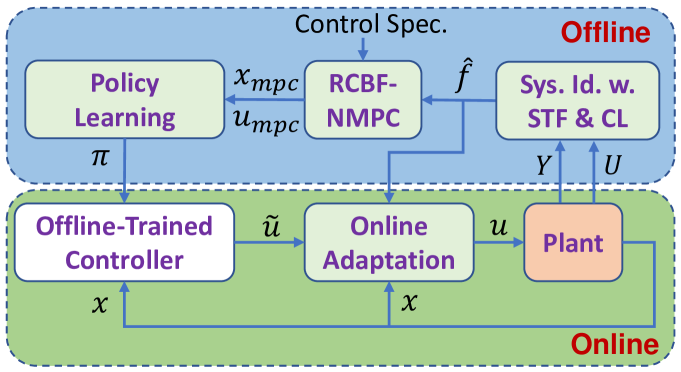
Figure 1: Schematic of online data-driven safe predictive control.

III Main Results

The developed data-driven safe predictive control pipeline is shown in Fig. 1. First, the discrete-time concurrent learning (CL) technique is integrated with the spatial temporal filter (STF) [9] for efficient nonlinear system identification with relaxed PE conditions. With the identified model and control specifications, the RCBF-based NMPC is exploited to optimize the system performance such that the safety is guaranteed despite the control policy learning error, the system identification error, and the unknown disturbances. A function approximator is then trained to approximate the RCBF-based NMPC policy for efficient online implementation, and an adaptation scheme is developed to minimize the performance loss due to the learning errors. The main components of the framework are detailed in the following subsections.

III-A Nonlinear System Identification with STF-based Concurrent Learning

In this subsection, we present a unified nonlinear system identification to obtain (5) and enable the nominal NMPC design. Specifically, we identify a nonlinear autoregressive exogenous model (NARX) using the input-output data as follows

$$y(k) =G(U_{d}(k),Y_{d}(k)),$$ (14)

$$U_{d}(k) =[u^{T}(k-1),u^{T}(k-2),\ldots,u^{T}(k-d_{u})],$$

$$Y_{d}(k) =[y^{T}(k-1),y^{T}(k-2),\ldots,y^{T}(k-d_{y})].$$

Here $d_{u}$ and $d_{y}$ are the input delay and the output delay, respectively, and $G$ is a nonlinear output prediction function.

Towards that end, we follow our prior work on STF-based system identification that exploits evolving clustering and recursive least squares to systematically decompose the nonlinear system into multiple local models and simultaneously identify the validity zone of each local model [9]. Specifically, let $U_{stf}(k)=[U_{d}(k),Y_{d}(k)]^{T}$, the nonlinear model (14) is expressed as a composite local model structure, where each local model has a certain valid operating regime, in the following form:

$$y(k) =F(U_{stf}(k),\omega(k);\Phi,\Psi)$$ (15)

$$=\sum\limits_{i=1}^{L}{\alpha}_{i}({U}_{stf}(k);\phi_{i},{\psi}_{i}){f}_{i}({U}_{stf}(k),\omega_{i}(k);{\phi}_{i}),$$

where ${f}_{i}({U}_{stf}(k),\omega_{i}(k);{\phi}_{i})$ is the $i$th local model that can take the form of a point, linear model, Markov chain, neural network etc, parameterized by ${\phi}_{i}$ in the presence of unstructured uncertainty $\omega_{i}(k)$. ${\alpha}_{i}({U}_{stf}(k);{\psi}_{i})$ is the weighting functions that interpolates the local models and is parameterized by ${\psi}_{i}$. It is based on a dissimilarity metric that combines clustering [40, 41, 42] and local model prediction error measures. $L$ is the number of local models, and $\Phi=[{\phi}_{1},{\phi}_{2},\ldots,{\phi}_{L}]$, $\Psi=[{\psi}_{1},{\psi}_{2},\ldots,{\psi}_{L}]$, and $\omega(k)=[w_{1}(k),w_{2}(k),\ldots,w_{L}(k)]$ are the collection of local model parameters, local interpolating function parameters, and unknown local unmodeled disturbance $w(k)$, respectively.

In particular, we consider linear local models and a softmax-like interpolation function:

$${f}_{i}({U}_{stf}(k),\omega_{i}(k);{\phi}_{i})={A}_{i}{U}_{stf}(k)+{b}_{i}+\omega_{i}(k),$$ (16)

$${\alpha}_{i}({U}_{stf}(k);{\psi}_{i},\phi_{i})=\frac{\exp(-D_{i}({U}_{stf});{\psi}_{i},\phi_{i}))}{\sum\limits_{j=1}^{L}{\exp(-D_{j}({U}_{stf});{\psi}_{i},\phi_{i}))}}.$$

Here $A_{i}\in\mathbb{R}^{n_{y}\times n_{U}}$ and $B_{i}\in\mathbb{R}^{n_{y}}$ are local model parameters, and $\omega_{i}(k)\in\mathbb{R}^{n_{y}}$ is the unstructured uncertainty for local model $i$. Moreover, ${\alpha}_{i}({U}_{stf}(k);{\psi}_{i},\phi_{i})$ resembles the softmax-like function, and $D_{i}({U}_{stf});{\psi}_{i},\phi_{i})$ is the dissimilarity metric that combines a Mahalanobis distance and the model residual [9]. Essentially, the STF uses evolving clusters of ellipsoidal shape as function bases for local model interpolation. Each local model ${f}_{i}$ is associated with an evolving cluster such that the clusters and the local model parameters are updated simultaneously. The readers are referred to [9] for more details about the STF.

The standard STF [9] uses the recursive least squares (RLS) to update the local model parameters $\{A_{i},b_{i}\}$, which requires a noise signal added to the system control input so that the PE condition is satisfied for learning error convergence. However, this will inevitably increase the complexity and may not be applicable in systems where the control inputs are not completely programmable. Therefore, in this subsection, we propose a discrete-time concurrent learning technique for the STF to relax the PE condition with a rank condition that is convenient for inspection and implementations.

Specifically, using the local linear models (LABEL:local_models), the nonlinear model (15) is rewritten as

$$y(k)=\sum\limits_{i=1}^{L}{\alpha}_{i}({U}_{stf}(k);{\psi}_{i})({A}_{i}{U}_{stf}(k)+{b}_{i}+\omega_{i}(k)),$$ (17)

which can be further written in the following compact form:

$$y(k)=\Phi\zeta({U}_{stf}(k),\alpha(k))+\omega(k),$$ (18)

where $\Phi=\left[A_{1},b_{1},\ldots,A_{L},b_{L}\right]\in\mathbb{R}^{n_{y}\times q}$, $\zeta({U}_{stf},\alpha)=\left[\alpha_{1}{U}^{T}_{stf},\,\alpha_{1},\ldots,\alpha_{L}{U}^{T}_{stf},\,\alpha_{L}\right]^{T}\in\mathbb{R}^{q}$, and $q=L(n_{U}+1)$. Moreover, the total unknown disturbance is given as $\omega=\alpha_{1}\omega_{1}+\ldots+\alpha_{L}\omega_{L}\in\mathbb{R}^{n_{y}}$, where $\|\omega(k)\|\leq\varepsilon$ and $\varepsilon=\alpha_{1}\varepsilon_{1}+\ldots+\alpha_{L}\varepsilon_{L}$ with $\varepsilon_{i}$ being the bound of $\omega_{i}$, i.e., $\|\omega_{i}(k)\|\leq\varepsilon_{i}$.

Therefore, the identified model can be represented as

$$\hat{y}(k)=\hat{\Phi}(k)\zeta({U}_{stf}(k),\alpha(k)),$$ (19)

where $\hat{\Phi}=\left[\hat{A}_{1},\hat{b}_{1},\ldots,\hat{A}_{L},\hat{b}_{L}\right]$. Thus, at each time step $k$, the system identification error is defined as

$${e}_{si}(k)=\hat{y}(k)-y(k)$$ (20)

$$\hskip 24.89615pt=\tilde{\Phi}(k)\zeta({U}_{stf}(k),\alpha(k))-\omega(k),$$

where $\tilde{\Phi}(k)=\hat{\Phi}(k)-\Phi$ describes the parameter identification errors. Note that the system identification error ${e}_{si}$ is measurable since the output $y$ is available for measurement.

The concurrent learning technique records past data and collects them in a history stack as

$$Z=\left[\zeta({U}_{stf}(k_{1}),\alpha(k_{1})),\ldots,\zeta({U}_{stf}(k_{s}),\alpha(k_{s}))\right],$$ (21)

where $k_{1},\ldots,k_{s}$ are the past historic recording time steps, and $s$ denotes the number of recorded data in the history stack. At the current time step $k$, the system identification error for the $j$th recorded sample $\zeta({U}_{stf}(k_{j}),\alpha(k_{j}))$ is given as

$${e}_{si}(k_{j})=\tilde{\Phi}(k)\zeta({U}_{stf}(k_{j}),\alpha(k_{j}))-\omega(k_{j}),\hskip 2.84526ptj=1,2,\ldots,s,$$ (22)

where $\tilde{\Phi}(k)$ is the parameter identification error at the current time step. Then, defining the normalizing signal $m(k)=\sqrt[]{\varrho+\zeta(k)^{T}\zeta(k)},\varrho>0$, one has

$$\bar{e}_{si}(k) =\tilde{\Phi}(k)\bar{\zeta}({U}_{stf}(k),\alpha(k))-\bar{\omega}(k),$$ (23)

$$\bar{e}_{si}(k_{j}) =\tilde{\Phi}(k)\bar{\zeta}({U}_{stf}(k_{j}),\alpha(k_{j}))-\bar{\omega}(k_{j}),$$

where $\bar{\zeta}(k)=\frac{\zeta(k)}{m(k)}$, $\bar{\omega}(k)=\frac{\omega(k)}{m(k)}$, $\bar{\zeta}(k_{j})=\frac{\zeta(k_{j})}{m(k_{j})}$, and $\bar{\omega}(k_{j})=\frac{\omega(k_{j})}{m(k_{j})}$.

Condition 1 (Rank Condition).

The number of linearly independent elements in the history stack $Z$ (LABEL:Recorded_Data) is the same as the dimension of $\zeta({U}_{stf},\alpha)$; i.e., $rank(Z)=q$.

Under Condition 1, it is obvious that the following inequalities hold:

$$H_{1}=\sum\limits_{j=1}^{s}\bar{\zeta}({U}_{stf}(k_{j}),\alpha(k_{j}))\bar{\zeta}^{T}({U}_{stf}(k_{j}),\alpha(k_{j}))>0,$$ (24)

$$H_{2}=\bar{\zeta}({U}_{stf}(k),\alpha(k))\bar{\zeta}^{T}({U}_{stf}(k),\alpha(k))+H_{1}>0.$$ (25)

Now, a discrete-time STF-based concurrent learning law is presented in the following theorem.

Theorem 1 (Discrete-Time STF-based Concurrent Learning).

Suppose Condition 1 is satisfied. Consider the nonlinear model (LABEL:Regressor_Format) and the identified model (LABEL:Regressor_Identified_Model). Then, the discrete-time concurrent learning law

$$\hat{\Phi}(k+1)=\hat{\Phi}(k)-\bar{e}_{si}(k)\bar{\zeta}^{T}({U}_{stf}(k),\alpha(k))\hskip 1.42262pt\Omega$$ (26)

$$\hskip 45.5244pt-\sum\limits_{j=1}^{s}\bar{e}_{si}(k_{j})\bar{\zeta}^{T}({U}_{stf}(k_{j}),\alpha(k_{j}))\hskip 1.42262pt\Omega$$

with the learning rate matrix $\Omega=rI_{q}$,

$$0<r<\frac{2\lambda_{min}(H_{2})}{\lambda_{max}^{2}(H_{2})}$$ (27)

guarantees that
i) the parameter identification errors $\tilde{\Phi}$ converges to zero when $\omega(k)=0$.
ii) the parameter identification errors $\tilde{\Phi}$ is uniformly ultimately bounded (UUB) when $\omega(k)\neq 0$.

Proof.

Consider the following Lyapunov function candidate:

$$V(k)=tr\{\tilde{\Phi}(k)\Omega^{-1}\tilde{\Phi}^{T}(k)\},$$ (28)

where $\tilde{\Phi}(k)$ and $\Omega=rI_{q}$ are the parameter identification errors and the learning rate matrix defined in (LABEL:System_Identification_Error) and (LABEL:Learning_rate), respectively. The derivative of the Lyapunov candidate (LABEL:Lyapunov_Candidate) in the discrete-time domain is obtained as

$$V(k+1)-V(k)$$ (29)

$$=tr\{\tilde{\Phi}(k+1)\Omega^{-1}\tilde{\Phi}^{T}(k+1)-\tilde{\Phi}(k)\Omega^{-1}\tilde{\Phi}^{T}(k)\}$$

$$=tr\{(\tilde{\Phi}(k+1)-\tilde{\Phi}(k))\Omega^{-1}(\tilde{\Phi}(k+1)+\tilde{\Phi}(k))^{T}\}$$

$$=tr\{(-\bar{e}_{si}(k)\bar{\zeta}^{T}(k)\hskip 1.42262pt\Omega-\sum\limits_{j=1}^{s}\bar{e}_{si}(k_{j})\bar{\zeta}^{T}(k_{j})\hskip 1.42262pt\Omega)\Omega^{-1}$$

$$\hskip 12.80373pt(-\bar{e}_{si}(k)\bar{\zeta}^{T}(k)\hskip 1.42262pt\Omega-\sum\limits_{j=1}^{s}\bar{e}_{si}(k_{j})\bar{\zeta}^{T}(k_{j})\hskip 1.42262pt\Omega+2\tilde{\Phi}(k))^{T}\}$$

$$=tr\{(-\tilde{\Phi}(k)H_{2}+H_{3})\hskip 1.42262pt(-\tilde{\Phi}(k)H_{2}\Omega+H_{3}\Omega+2\tilde{\Phi}(k))^{T}\},$$

where $H_{3}=\bar{\omega}(k)\bar{\zeta}^{T}(k)+\sum\limits_{j=1}^{s}\bar{\omega}(k_{j})\bar{\zeta}^{T}(k_{j})$, and $\|H_{3}\|\leq\bar{\varepsilon}_{n}$. Here, one can obtain $\bar{\varepsilon}_{n}$ using the bound of $\omega$. Now, one has

$$V(k+1)-V(k)$$ (30)

$$=tr\{\tilde{\Phi}(k)P_{1}\tilde{\Phi}^{T}(k)+\tilde{\Phi}(k)P_{2}+P_{3}\tilde{\Phi}^{T}(k)+P_{4}\},$$

where $P_{1}=H_{2}\Omega^{T}H^{T}_{2}-2H_{2}$, $P_{2}=-H_{2}\Omega^{T}H^{T}_{3}$, $P_{3}=-H_{3}\Omega^{T}H^{T}_{2}+2H_{3}$, and $P_{4}=H_{3}\Omega^{T}H^{T}_{3}$. Thus, one has

$$V(k+1)-V(k)\leq Q_{1}\|\tilde{\Phi}(k)\|^{2}+Q_{2}\|\tilde{\Phi}(k)\|+Q_{3},$$ (31)

where $Q_{1}=r\lambda^{2}_{max}(H_{2})-2\lambda_{min}(H_{2})$, $Q_{2}=r\lambda_{min}(H_{2})\bar{\varepsilon}_{n}$ $+r\lambda_{min}(H_{2})\bar{\varepsilon}_{n}+2\bar{\varepsilon}_{n}$, and $Q_{3}=r\bar{\varepsilon}^{2}_{n}$. Now, using (LABEL:Learning_rate), it is clear that $Q_{1}<0$; therefore, using (LABEL:Lyapunov_Candidate), one has the following inequality when $\omega(k)=0$:

$$V(k+1)-V(k)\leq Q_{1}\|\tilde{\Phi}(k)\|^{2}\leq r\hskip 1.42262ptQ_{1}V(k)<0.$$ (32)

Thus, the parameter identification errors $\tilde{\Phi}$ converge to zero. Consequently, from (LABEL:System_Identification_Error), the convergence of $\tilde{\Phi}$ indicates that the system identification error $e_{si}$ converges to zero. This completes the proof of the first part.

Now, for $\omega(k)\neq 0$, since $\|\tilde{\Phi}(k)\|\geq 0$, $Q_{1}<0$, $Q_{2}\geq 0$, and $Q_{3}\geq 0$, the only valid non-negative root of (LABEL:Lyapunov_Candidate_Derivative_3) is

$$\tilde{\Phi}_{b}=\frac{-Q_{2}-\sqrt{Q^{2}_{2}-4Q_{1}Q_{3}}}{2Q_{1}}.$$ (33)

Thus, when $\|\tilde{\Phi}(k)\|>\tilde{\Phi}_{b}$, one has

$$V(k+1)-V(k)<0,$$ (34)

which makes $\tilde{\Phi}(k)$ to enter and stay in the compact set $S_{\tilde{\Phi}}=\{\tilde{\Phi}:\|\tilde{\Phi}\|\leq\tilde{\Phi}_{b}\}$; therefore, one can conclude that the system identification error $e_{si}$ converges to a small region around zero using (LABEL:System_Identification_Error). This completes the proof of the second part. ∎

Remark 1 (System Identification).

Theorem 1 presents a learning law to guarantee a reasonable performance for the proposed STF-based concurrent learning. We investigate two cases: i) the real system without any external disturbances, and ii) the real system with external disturbances. For the first case, i.e., $\omega(k)=0$, we prove that the system identification error converges to zero, and the real system is identified perfectly. For the second case with $\omega(k)\neq 0$, although it is known that the system identification error does not converge to zero, we prove that it is uniformly ultimately bounded (UUB), which means that the system identification error converges to a small region around zero (LABEL:parameter_bound). Thus, it is clear that the real system is identified with a reasonable performance even in the presence of external disturbances. To see how we use the learning law in the proposed identifier, we present Algorithm 1 and the corresponding explanations later.

Remark 2 (Rich Data).

The singular value maximizing approach [43] is used for recording rich data in the history stack (LABEL:Recorded_Data). When Condition 1 is satisfied, the richness of the history stack (LABEL:Recorded_Data) suffices to achieve the results in Theorem 1. However, replacing new rich data with old data in the history stack can improve the learning performance if the new data increases $\lambda_{min}(H_{2})$ and/or decreases $\lambda_{max}(H_{2})$, leading to a reduced convergence time.

Remark 3 (Comparison).

As compared to [9], the regressor vector $\zeta({U}_{stf},\alpha)$ has to be persistently exciting (see Definition 2), imposing conditions on past, current, and future regressor vectors that is difficult or impossible to verify online. Instead, Condition 1 only deals with a subset of past data, which makes it easy to monitor. Also, it is convenient to check whether replacing new data will increase $\lambda_{min}(H_{2})$ and/or decrease $\lambda_{max}(H_{2})$ to reduce the convergence time. In comparison with [38], the STF-based concurrent learning does not require the measurement or estimation of the derivatives of the system states (1). In comparison with [37, 36], the STF-based concurrent learning does not require a filter regressor for obviating the derivatives of the system states. Compared to our previous work [44], the discrete-time concurrent learning technique is extended to handle both structured and unstructured uncertainties.

The steps for transferring from the STF model structure to the state-space form are provided in Appendix A. For the offline system identification and control policy learning, using Theorem 1 and Appendix A, one can see that $e_{s}$ and $e_{c}$ converge to zero when $\omega(k)=0$ and are UUB when $w\neq 0$. Therefore, after learning process, one can conclude that $e_{s}$ and $e_{c}$ are zero for $w=0$ and around zero for $w\neq 0$.

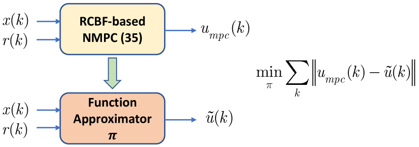
Figure 2: Schematic of NMPC policy function approximation.

III-B Data-Driven Safe Predictive Control with Function Approximations

With the identified STF model, one can use the steps in Appendix A to transform the STF model to a state-space model and implement the NMPC (LABEL:NMPC). However, in many real-time engineering systems, it is very computationally expensive, especially for nonlinear systems, to implement the NMPC. Therefore, in this section, we develop a data-driven safe predictive control framework using policy function approximators. As illustrated in Fig. 2, we utilize a function approximator (e.g., neural network, Gaussian process regression, or STF) to approximate the NMPC policy, which can be viewed as a mapping from the state $x(k)$ and the reference $r(k)$ to the control $u_{mpc}(k)$. The function approximator can be obtained by minimizing the accumulated loss, i.e., the difference between the NMPC $u_{mpc}$ and the predicted control $\tilde{u}(k)$.

With the trained function approximator, the online control computation is greatly reduced as only simple algebraic computations are needed as compared to the original constrained nonlinear optimization. Due to the control policy learning error, the system identification error, and the unknown disturbances, the constraints in (2) may not be satisfied. Therefore, we develop a RCBF-based NMPC such that the function-approximated control policy can still guarantee constraint satisfaction in the presence of $e_{c}$, $e_{s}$, and $w$.

Specifically, suppose that the dynamics drifting (LABEL:identification_error) due to the system identification error and the control policy learning error are bounded by $\varepsilon_{s}$ and $\varepsilon_{c}$, respectively, i.e., $\|e_{s}(k)\|\leq\varepsilon_{s}$ and $\|e_{c}(k)\|\leq\varepsilon_{c}$ for all time steps $k$. Note $\varepsilon_{s}$ and $\varepsilon_{c}$ can be obtained by empirically evaluating the bounds using trajectories from design of experiments. Consider the state constraints $X=\{x\in\mathbb{R}^{n}:h(x)\leq 0\}$. We modify the nominal NMPC in (LABEL:NMPC) with the following RCBF-based NMPC design:

$$(\mathbf{x}^{*},\mathbf{u}^{*},\mathbf{\gamma}^{*})=\underset{\mathbf{\hat{x}},\mathbf{u},\mathbf{\gamma}}{\arg\min}\hskip 2.84526ptJ_{N}(\mathbf{\hat{x}},\mathbf{u})+\varphi(\gamma)$$ (35)

$$s.t.\quad\hat{x}(k+1)=\hat{f}(\hat{x}(k),u(k)),\quad\hat{y}(k)=g(\hat{x}(k)),$$

$$\hskip 24.18483pt\hat{x}(0)=\hat{x}_{0},\quad u(k)\in U,$$

$$\hskip 24.18483pth(\hat{x}(k+1))\leq(1-\gamma)h(\hat{x}(k))-\gamma\eta(\varepsilon_{w}+\varepsilon_{s}+\varepsilon_{c}),$$

$$\hskip 24.18483pt0<\gamma\leq 1,$$

where $\varphi(\gamma)=P\gamma^{2}$ is a regularization term on the optimal variable $\gamma$ with $P>0$ being a weighting factor. The following theorem shows that approximating the NMPC policy based on the RCBF-based NMPC (LABEL:RCBF-based_NMPC), particularly the last constraint, can robustly guarantee constraint satisfaction when using the function-approximated control policy $\tilde{u}(k)$ for online controls.

The following theorem enables us to consider a robust safety constraint using the identified model such that the nonlinear system (1) is safe in the presence of the model uncertainties (i.e., $w,e_{s},e_{c}$). If the optimization problem (35) is feasible, it is guaranteed to give a control input that satisfies the true CBF constraint (9).

Theorem 2 (Robust Constraint Satisfaction).

Consider the real system (1), the identified model (5), the drift dynamics error (LABEL:identification_error), and the safe set (LABEL:Safe_set). Define $h_{r}(\hat{x})=h(\hat{x})+\eta(\varepsilon_{w}+\varepsilon_{s}+\varepsilon_{c})$ as the RCBF. The safety constraint

$$h(\hat{x}(k+1))\leq(1-\gamma)h(\hat{x}(k))-\gamma\eta(\varepsilon_{w}+\varepsilon_{s}+\varepsilon_{c})$$ (36)

guarantees that the safe set $S$ is forward invariant in the presence of control learning error $e_{c}$, system identification error $e_{s}$, and unknown disturbance $w$.

Proof.

For notational simplicity, we use $x_{k}$ to denote $x(k)$ in the following equation. Using the mean value theorem, the identified model (5), and the nonlinear system (11), one has

$$h(x_{k})=h(\hat{x}_{k}+(x_{k}-\hat{x}_{k}))$$ (37)

$$\hskip 24.18483pt=h(\hat{x}_{k})+(h(x_{k})-h(\hat{x}_{k}))$$

$$\hskip 24.18483pt\leq h(\hat{x}_{k})+\left|h(x_{k})-h(\hat{x}_{k})\right|$$

$$\hskip 24.18483pt\leq h(\hat{x}_{k})+\eta\left\|x_{k}-\hat{x}_{k}\right\|$$

$$\hskip 24.18483pt\leq h(\hat{x}_{k})+\eta\left(\left\|w_{k-1}\right\|+\left\|{e_{fs}}_{k-1}\right\|+\left\|{e_{fc}}_{k-1}\right\|\right)$$

$$\hskip 24.18483pt\leq h(\hat{x}_{k})+\eta(\varepsilon_{w}+\varepsilon_{s}+\varepsilon_{c})$$

$$\hskip 24.18483pt=h_{r}(\hat{x}_{k}).$$

Thus, $h_{r}(\hat{x}_{k})\leq 0$ implies that $h(x_{k})\leq 0$.
Using (8), the following safety constraint guarantees that $h_{r}(\hat{x}(k))\leq 0$ for all time steps $k$ as

$$\triangle h_{r}(\hat{x}(k))\leq-\gamma h_{r}(\hat{x}(k)).$$ (38)

Now, using (LABEL:Mean_Value), one can rewrite (LABEL:Robust_CBF_condition) as

$$h(\hat{x}(k+1))-h(\hat{x}(k))\leq-\gamma\left(h(\hat{x}(k))+\eta(\varepsilon_{w}+\varepsilon_{s}+\varepsilon_{c})\right),$$ (39)

which is (LABEL:RCBF_Constraint), and the proof is completed. ∎

Remark 4 (Relaxed RCBF).

In the optimization problem (LABEL:RCBF-based_NMPC), if $\gamma$ becomes relatively small, the sublevel set of the RCBF $h$ will be smaller, and the system tends to be safer; however, the intersection between the reachable set and the sublevel set might be infeasible. When $\gamma$ becomes larger, the sublevel set will be increased in the state space, which makes the optimization problem more likely to be feasible; however, the RCBF constraint might not be active during the optimization. If $\gamma=1$, the relaxed RCBF constraint becomes equivalent to a simple distance constraint; consequently, the NMPC needs a longer horizon of prediction to generate an expected system safety performance in the closed-loop trajectory. Therefore, it is not recommended to set a relatively too small value for $P$, which would over-relax the RCBF constraint and make the optimized value $\gamma$ closer to 1.

Remark 5 (Feasibility).

The recursive feasibility is generally not guaranteed for the MPC in the presence of both safety constraint and control input constraint [45, 46]. In [35], the control input constraint is relaxed to ensure the feasibility of the optimization problem with the safety constraint. However, in this paper, the decay rate of the RCBF is relaxed from a fixed value to an optimal variable so that it improves both safety and feasibility of the NMPC problem (LABEL:RCBF-based_NMPC). Formal guarantee on the recursive feasibility in the presence of both safety and control input constraints requires more analysis and will be addressed in our future work. It is worth noting that even in the absence of control input constraint, the optimization problem (LABEL:RCBF-based_NMPC) will be infeasible if the model uncertainties in the RCBF constraint are too high. The optimization problem (LABEL:RCBF-based_NMPC) is formulated with an identified model, and the proposed offline system identification technique is utilized to well capture the system dynamics, ensuring that the model uncertainties will be varying within bounded compatible sets online (i.e., $\varepsilon_{w},\varepsilon_{s},\varepsilon_{c}$). In particular, under the assumption that the external disturbance $w$ is bounded (see Assumption 1), our STF-based concurrent learning ensures that the bounds on the system identification error and the control learning error are zero and small values close to zero for $w=0$ and $w\neq 0$, respectively (see Theorem 1 and Remark 1). Therefore, thanks to Theorem 1, the RCBF constraint (LABEL:RCBF_Constraint) will be satisfied, and the optimization problem (LABEL:RCBF-based_NMPC) without control input constraints will be feasible at all times.

Now, the proposed discrete-time STF-based concurrent learning is used again to learn the RCBF-based NMPC policy (LABEL:RCBF-based_NMPC), which $(x(k),r(k:k+N))$ and $u_{mpc}(k)$ are respectively considered as the input and the output of the policy.

III-C Online Adaptive Control Policy

Although the function-approximated control policy $\tilde{u}(k)$ may already lead to a reasonable closed-loop performance for many cases, one can see a performance loss for a system due to i) the choice of the hyperparameters that decide the architecture of the STF-based identification law and the function-approximated control policy, and ii) insufficient training data in some regions of the feasible state space. To minimize this performance loss, caused by $e_{c}$, $e_{s}$, and $w$, it may be desirable to adapt $\tilde{u}(k)$ online.

Corollary 1 (Steady-State Optimization Problem [23]).

Using the RCBF-based NMPC policy, a unique equilibrium pair $(x_{e},u_{e})$ minimizes the steady-state optimization problem

$$(\mathbf{x}_{e},\mathbf{u}_{e},\mathbf{\gamma}_{e})=\underset{\mathbf{\hat{x}},\mathbf{u},\mathbf{\gamma}}{\arg\min}\hskip 2.84526ptl(\hat{x},u,\gamma)$$ (40)

$$s.t.\quad\hat{x}=\hat{f}(\hat{x},u),\quad\hat{y}=g(\hat{x})$$

$$\hskip 24.18483ptu\in U,$$

$$\hskip 24.18483pth(\hat{x})\leq(1-\gamma)h(\hat{x})-\gamma\eta(\varepsilon_{w}+\varepsilon_{s}+\varepsilon_{c}),$$

where $l(\hat{x},u,\gamma)=\phi(\hat{x},u,\hat{y},r)+\psi(\hat{x},\hat{y},r)+\varphi(\gamma)$ represents the steady-state cost function.                                      $\square$

Condition 2 (Steady-State Function-Approximated Control).

$(x^{\prime}_{e},u^{\prime}_{e})$ is the asymptotically stable equilibrium point of the nominal model (5) under the approximated control policy $\tilde{u}$.

Lemma 1 (Modified Steady-State Optimization Problem).

For the equilibrium point $(x_{e},u_{e})$, the steady-state optimization problem (LABEL:Steady-State_NMPC) can implicitly be written as

$$\mathbf{u}_{e}=\underset{\mathbf{u}}{\arg\min}\hskip 2.84526pt\tilde{l}(u)$$ (41)

$$s.t.\quad\tilde{h}(u)\leq 0,$$

where the constraints of the optimization problem (LABEL:Steady-State_NMPC) are collectively denoted as $\tilde{h}(u)$.

Proof.

Let $\hat{x}(k)$ and $\tilde{u}(k)$ denote the nominal trajectory using the function-approxiamted control policy. Thus, the nominal trajectory for the RCBF-based NMPC policy (LABEL:RCBF-based_NMPC) is expressed as

$$\hat{x}_{mpc}(k)=\hat{x}(k)+\delta\hat{x}(k),$$ (42)

$$u_{mpc}(k)=\tilde{u}(k)+\delta u(k),$$

where $\delta u(k)$ represents the difference between the NMPC and function-approximated control policy at each time step $k$, and $\delta\hat{x}(k)$ denotes the resulting change in the states. Using the nominal model (5), one has

$$\delta\hat{x}(k+1)=\hat{f}_{\hat{x}}(k)\delta\hat{x}(k)+\hat{f}_{u}(k)\delta u(k),$$ (43)

$$\delta l(k)=l_{\hat{x}}(k)\delta\hat{x}(k)+l_{u}(k)\delta u(k),$$

where $\hat{f}_{\hat{x}}(k)$, $\hat{f}_{u}(k)$, $l_{\hat{x}}(k)$, and $l_{u}(k)$ are partial derivatives with respect to $\hat{x}$ and $u$, respectively, and obtained using $\hat{x}(k)$ and $\tilde{u}(k)$.

Now, it is clear that $\delta\hat{x}(k+1)=\delta\hat{x}(k)$ for the steady-state condition; therefore, one has

$$\delta\hat{x}(k)=(I_{n}-\hat{f}_{\hat{x}}(k))^{-1}\hat{f}_{u}(k)\hskip 2.13394pt\delta u(k),$$ (44)

and

$$\delta l(k)=(l_{\hat{x}}(k)(I_{n}-\hat{f}_{\hat{x}}(k))^{-1}\hat{f}_{u}(k)+l_{u}(k))\hskip 2.13394pt\delta u(k).$$ (45)

Using (45), one has $\delta\tilde{l}(u)=(l_{\hat{x}}(I_{n}-\hat{f}_{\hat{x}})^{-1}\hat{f}_{u}+l_{u})$ and can obtain $\tilde{l}(u)$. Similarly, $\tilde{h}(u)$ is obtained using the same process. This completes the proof. ∎

Now, consider $\tilde{x}=\hat{x}-x$ and define an auxiliary variable $s$ as

$$s(k)=\Gamma\tilde{x}(k),$$ (46)

where $\Gamma\in\mathbb{R}^{m\times n}$ is designed such that $\Gamma\hat{f}_{u}\in\mathbb{R}^{m\times m}$ is a diagonal matrix. The following theorem presents the proposed online correction scheme, including an KKT adaptation and an ancillary feedback control.

Theorem 3 (Online Adaptive Control Policy).

Considering the real system (1), the nominal model (5), Corollary 1, Lemma 1, and the auxiliary variable $s$ (46), the online adaptation policy

$$u(k)=\tilde{u}(k)+\delta u(k)+K(\hat{x}(k),x(k)),$$ (47)

$$\delta u(k)\approx\delta u(k-1)-K_{0}\begin{bmatrix}\tilde{h}_{a}(u(k-1))\\ N^{T}\delta\tilde{l}(u(k-1))\end{bmatrix},$$

$$K_{0}=\begin{bmatrix}\delta\tilde{h}_{a}(u(k-1))\\ N^{T}\delta^{2}\tilde{l}(u(k-1))\end{bmatrix}^{-1},$$

$$K(\hat{x}(k),x(k))=\frac{1}{\Gamma\hat{f}_{u}(\hat{x}(k),\tilde{u}_{mpc}(k))}(\Upsilon s(k)+\Gamma\varepsilon_{w}+\Gamma\varepsilon_{s}).$$

with the design matrix $\Upsilon\in\mathbb{R}^{m\times m}$ $(0\leq\Upsilon_{ii}<1,\hskip 2.84526pti=1,...,m)$ and $\tilde{u}_{mpc}(k)=\tilde{u}(k)+\delta u(k)$ minimizes the performance loss due to the control learning error, the system identification error, and the unknown disturbance.

Proof.

The first part of the proof focuses on minimizing the performance loss for the nominal model (5) due to the control learning error. Considering Corollary 1 and Lemma 1, one can conclude that $(x_{e},u_{e})$ is an asymptotically stable equilibrium point of the nominal model under the RCBF-based NMPC policy. Hence, $u_{mpc}$ satisfies the KKT conditions of (LABEL:Modified_Steady-State_NMPC), which are expressed as

$$\delta\tilde{l}(u)+\delta\tilde{h}_{a}(u)^{T}\lambda=0,$$ (48)

$$\lambda^{T}\tilde{h}(u)=0,$$

where $\tilde{h}_{a}(u)$ denotes the active constraints, and $\lambda\geq 0$ is the Lagrange multiplier. Now, one can rewrite (LABEL:KKT) as

$$\mathcal{A}^{T}\delta\tilde{l}(u)=0,$$ (49)

$$\tilde{h}_{a}(u)=0,$$

where $\mathcal{A}$ lies in the null space of the active constraint variation, i.e., $\mathcal{A}^{T}\delta\tilde{h}_{a}(u)^{T}=0$.

Due to the control learning error $e_{c}$, one may have $(x^{\prime}_{e},u^{\prime}_{e})\neq(x_{e},u_{e})$; therefore, the goal is that the function-approximated control policy $\tilde{u}(k)$ is adapted online such that it guarantees $(x^{\prime}_{e},u^{\prime}_{e})=(x_{e},u_{e})$. Using Lemma 1, it is clear that $(x^{\prime}_{e},u^{\prime}_{e})$ does not satisfy the KKT conditions (LABEL:KKT_2) if $(x^{\prime}_{e},u^{\prime}_{e})\neq(x_{e},u_{e})$. Thus, the deviation from the KKT condition (LABEL:KKT_2) indicates asymptotic performance loss stemming from the RCBF-based NMPC policy approximation. Consequently, $\delta u$ minimizes the asymptotic performance loss due to $e_{c}$, and the gain $K_{0}$ is chosen such that it does not significantly affect the dynamics, but adjusts the asymptotic performance. Therefore, the first part of the proof is completed.

Now, we have a reasonable performance for the nominal model under the function-approximated control policy $\tilde{u}(k)$; however, the performance loss still exists for the real system (1) due to the system identification error and the unknown disturbance. Considering the nominal model (5) under $\tilde{u}_{mpc}$, one has

$$\tilde{x}(k+1)=\hat{x}(k+1)-x(k+1)$$ (50)

$$=\hat{f}(\hat{x}(k),\tilde{u}_{mpc}(k))-f(x(k),u(k))-w(k)$$

$$=\hat{f}(\hat{x}(k),\tilde{u}_{mpc}(k))-\hat{f}(\hat{x}(k),u(k))+e_{s}(k)-w(k)$$

$$=\hat{f}_{u}(\hat{x}(k),\tilde{u}_{mpc}(k))\hskip 1.99168pt(\tilde{u}_{mpc}(k)-u(k))+e_{s}(k)-w(k)$$

$$=-\hat{f}_{u}(\hat{x}(k),\tilde{u}_{mpc}(k))\hskip 1.99168ptK(\hat{x}(k),x(k))+e_{s}(k)-w(k).$$

Now, the Lyapunov function candidate is considered as

$$V(k)=s(k)^{T}s(k),$$ (51)

where $V(k)$ is a positive definite function. The derivative of the Lyapunov candidate (51) in the discrete-time domain is obtained as

$$V(k+1)-V(k)=s(k+1)^{T}s(k+1)-s(k)^{T}s(k).$$ (52)

Using (46)-(LABEL:x_tilde), one has

$$s(k+1)=\Gamma\tilde{x}(k+1)$$ (53)

$$=-\Upsilon s(k)-\Gamma\varepsilon_{w}-\Gamma\varepsilon_{s}+\Gamma e_{f}(k)-\Gamma w(k)$$

$$\leq-\Upsilon s(k)-\Gamma\varepsilon_{w}-\Gamma\varepsilon_{s}+\Gamma\|e_{f}(k)\|+\Gamma\|w(k)\|$$

$$\leq-\Upsilon s(k).$$

Using (52) and (LABEL:s_2), considering $P=I_{m}-\Upsilon^{T}\Upsilon$, one has

$$V(k+1)-V(k)\leq-s(k)^{T}Ps(k)$$ (54)

$$\hskip 72.26997pt\leq-\lambda_{min}(P)V(k)$$

$$\hskip 72.26997pt<0.$$

Consequently, one can conclude that $\delta u(k)$ minimizes the difference between $u_{mpc}$ and $\tilde{u}$, and $K(\hat{x},x)$ keeps the actual states $x$ of the real system around the nominal trajectory $\hat{x}$ under $\tilde{u}_{mpc}$; therefore, $K(\hat{x},x)$ minimizes the performance loss due to system identification error $e_{s}$ and the unkknown disturbance $w$. This completes the proof. ∎

Remark 6 (KKT Condition).

To develop the proposed adaptation law (LABEL:Online_Adaptation), Condition 2 must be satisfied for the nominal model, which means that its closed-loop performance under the function-approximated control policy $\tilde{u}(k)$ converges to an equilibrium point $(x^{\prime}_{e},u^{\prime}_{e})$, but it may not be the desired equilibrium point $(x_{e},u_{e})$ from the RCBF-based NMPC policy $u_{mpc}(k)$ because of the policy approximation error. When training $\tilde{u}(k)$ using the RCBF-based NMPC policy $u_{mpc}(k)$, one wants the equilibrium solution to converge to the same limit point $(x_{e},u_{e})$, where the KKT conditions hold. Consequently, we adapt $\tilde{u}(k)$ online to ensure that $(x^{\prime}_{e},u^{\prime}_{e})$ satisfies the KKT conditions and make $(x^{\prime}_{e},u^{\prime}_{e})=(x_{e},u_{e})$.

Remark 7 (Offline Probabilistic Verification).

To guarantee that Condition 2 is satisfied, using the offline data-driven safe predictive control, the nominal model is simulated for $N_{v}$ randomly selected initial states in the training data range as

$$N_{v}\geq\frac{\log\frac{1}{\kappa}}{\log\frac{1}{1-\epsilon}},$$ (55)

where $\epsilon\in(0,1)$ and $\kappa\in(0,1)$ denote the accuracy and confidence of the offline probabilistic verification. If all $N_{v}$ closed-loop trajectories are stable ($E=0$), one can conclude that the nominal model under the function-approximated control policy converges to $(x^{\prime}_{e},u^{\prime}_{e})$ for all initial states with the probability [23]

$$Pr\{Pr\{E=0\}\geq 1-\epsilon\}\geq 1-\kappa.$$ (56)

However, if any closed-loop trajectory from $N_{v}$ samples is unstable, the control learning procedure must be repeated.

Remark 8 (Safety and Performance).

Using Theorem 3, it is clear that the online adaptive control policy (LABEL:Online_Adaptation) keeps the actual states $x$ around the nominal trajectory $\hat{x}$ under $\tilde{u}_{mpc}$. Therefore, using the fourth line in (LABEL:Mean_Value), one can make sure that the online adaptive control policy improves the safety for the real system. Moreover, since the performance loss caused by $e_{c}$, $e_{s}$, and $w$ is mitigated, the online adaptive control policy (LABEL:Online_Adaptation) has better performance than the function-approximated control policy $\tilde{u}(k)$ and the RCBF-based NMPC policy (LABEL:RCBF-based_NMPC) for online controls.

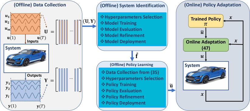
Figure 3: Sequence of Steps of online data-driven safe predictive control.

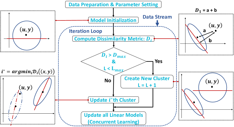
Figure 4: Sequence of Steps of discrete-time STF-based Concurrent Learning: i) First cluster-model is initialized for the first I/O data, ii) For next data, the dissimilarity metric is computed to either create a new cluster-model or update one of the existing ones, iii) For each iteration, all linear models are updated using the CL, and iv) The process is repeated until all training I/O data is used.

Remark 9 (Computational Cost).

The online data-driven safe predictive control is much less computationally costly than the RCBF-based NMPC problem (LABEL:RCBF-based_NMPC) since the proposed control policy learns the NMPC policy while keeping the real system safe; however, it does not need to solve an optimization problem at each time step $k$ (only algebraic computations are needed). In comparison with our previous work [44], the RCBF is extended to guarantee system safety in the presence of not only the system identification error and the external disturbance but also the control learning error. Therefore, we have removed the QP safety filter from the algorithm. Moreover, the proposed online adaptive control policy enables us to minimize the performance loss; thus, we do not need to consider a switching criteria for returning the NMPC. These two contributions effectively reduce the computational cost for the proposed algorithm.

The procedure for determining the online data-driven safe predictive control is summarized in Fig. 3 and Algorithm 1. Fig. 3 shows a flowchart that represents the sequence of the steps of the proposed data-driven control framework, and Algorithm 1 describes each step in the flowchart. Moreover, Fig. 4 presents a flowchart that describes the step of model training using the discrete-time STF-based concurrent learning, and the readers are referred to see Algorithms 1 and 2 in [9] for more details about the sequence of the steps of the STF framework. It is worth noting that we have modified the Algorithm 2 in [9] such that we use the concurrent learning law instead of the recursive least squares (RLS) law to remove the PE requirement.

Algorithm 1 Online data-driven safe predictive control

I. Offline System Identification:
1- Data Collection: Collect the raw input/output data $(u/y)$ from the real system.
2- Data Processing: Process the data to prepare it for model learning, which includes data normalization and data partitioning to training data and validation data.
3- Hyperparameters Selection: Determine the appropriate STFs’ hyperparameters to use for model learning, which can be done through trial and error, feature selection, or genetic algorithm (GA).
4- Model Training: Train a model on the processed data using the discrete-time STF-based concurrent learning on the training data to identify the real system and obtain the identified model (5).
5- Model Evaluation: Evaluate the performance of the trained model using the best fitting rate, which analyzes the goodness of fit between the measured output and the simulated output of the trained model on the validation data.
6- Model Refinement: If the performance of the trained model is not satisfactory, refine the model by adjusting the hyperparameters.
7- Model Deployment: Once the model is trained and validated, it can be deployed for real-world use. This may involve retraining the trained model with new data, which may need updating STFs’ hyperparameters.
II. Offline NMPC Learning: Using the identified model (5), we collect raw data from the RCBF-based NMPC (LABEL:RCBF-based_NMPC) such that $x,r$ and $u$ are considered as the input and the output of the control policy. Doing same procedure as the step I (i.e., offline system identification), we use the discrete-time STF-based concurrent learning as a function approximator to learn the RCBF-based NMPC policy. Once the policy is trained and validated, it can be deployed for real-world use. This may involve retraining the trained policy with new data, which may need updating STFs’ hyperparameters.
III. Online Adaptation: The adaptation law (LABEL:Online_Adaptation) is used online to minimize the performance loss caused by the control learning error, the system identification error, and the unknown disturbance.

IV Simulation Results

In this section, two simulation examples are considered to demonstrate the effectiveness of the proposed online data-driven safe predictive control. The simulation results are presented for a cart-inverted pendulum and a gasoline engine controls. The cart-inverted pendulum has a known model, where we use it for NMPC to compare its result with the proposed online data-driven safe predictive control. However, there is not any known model for the gasoline engine vehicle; thus, we use the collected data from the system to identify a nominal model for the NMPC and compare its result with the proposed online data-driven safe predictive control.

Figure 5: Cart-inverted pendulum.

IV-A Cart-Inverted Pendulum

As shown in Fig. 5, an inverted pendulum mounted to a cart is modeled in continuous-time domain as

$$\ddot{z}=\frac{F-{K}_{d}\dot{z}-{m}_{pend}(L{\dot{\theta}}^{2}\sin(\theta)-g\sin(\theta)\cos(\theta))}{{m}_{cart}+{m}_{pend}{\sin}^{2}(\theta)},$$ (57)

$$\ddot{\theta}=\frac{\ddot{z}\cos(\theta)+g\sin(\theta)}{L},$$

where $z$ and $\theta$ are the cart position and the pendulum angle, respectively. ${m}_{cart}=5kg$, ${m}_{pend}=1kg$, $L=2m$, ${K}_{d}=10Ns/m$, and $g=9.81m/s^{2}$ present the cart mass, the pendulum mass, the length of the pendulum, the damping parameter, and the gravity acceleration, respectively. The system is controlled by a variable force $F$, and the model (LABEL:Cart-inverted_pendulum) is discretized with a sampling time $T=0.1s$.

Now, the states and the outputs of the model (LABEL:Cart-inverted_pendulum), the safety constraint, and the input constraint are considered as

$$x={[{x}_{1},{x}_{2},{x}_{3},{x}_{4}]}^{T}={[z,\dot{z},\theta,\dot{\theta}]}^{T},$$ (58)

$$y={[{x}_{1},{x}_{3}]}^{T}={[z,\theta]}^{T},$$ (59)

$$-5\leq z\leq 5,$$ (60)

$$-100\leq F\leq 100.$$ (61)

Using (LABEL:Safe_set), (LABEL:Mean_Value), and (60), the CBF and the RCBF are considered as

$$h(x)=\left\|x\right\|-0.5,$$ (62)

$${h}_{r}(\hat{x})=\left\|\hat{x}\right\|-0.5+\eta(\varepsilon_{w}+\varepsilon_{s}+\varepsilon_{c}),$$ (63)

where $\eta=1$, $\varepsilon_{w}=0.01$, $\varepsilon_{s}=0.01$, and $\varepsilon_{c}=0.01$ are considered in (63). Using (58) and (60), it is clear that the RCBF is only considered for $x_{1}$.

According to Algorithm 1, the online data-driven safe predictive control is applied to the discrete-time version of the cart-inverted pendulum (LABEL:Cart-inverted_pendulum), which yields 1) 97.54% accuracy for 30000 training data with 10 clusters and local linear models in the offline system identification, and 2) 98.66% accuracy for 100000 training data with 20 clusters and local linear models in the offline RCBF-based NMPC learning.

For the proposed online data-driven safe predictive control, the nonlinear system (LABEL:Cart-inverted_pendulum) is considered in the presence of disturbance ${w}(k)=-0.01+0.02\times rand(4,1)$. Fig. 6 depicts the control input signal $F$ using the RCBF-based NMPC, the offline data-driven safe predictive control, and the online data-driven safe predictive control with four future state predictions $N=4$ for the cart-inverted pendulum. For this example, it should be mentioned that the RCBF-based NMPC policy (LABEL:RCBF-based_NMPC) works with the well-known model (LABEL:Cart-inverted_pendulum); however, we adapt it using the feedback controller in (LABEL:Online_Adaptation) to minimize the performance loss caused by the considered external disturbance ${w}(k)$. Moreover, one can see that the proposed online adaptive control policy corrects the offline data-driven safe predictive control and approximates the RCBF-based NMPC policy better. Fig. 7 shows that the outputs of the cart-inverted pendulum (LABEL:Cart-inverted_pendulum) converge to zero using three control schemes whereas one can see the performance loss if only the offline data-driven safe predictive control is used. From Figs. 6 and 7, one can see that Condition 2 is satisfied such that the system converges to an equilibrium point $(x^{\prime}_{e},u^{\prime}_{e})$ using the offline data-driven safe predictive control; however, it is not same as the equilibrium point $(x_{e},u_{e})$ obtained by the RCBF-based NMPC policy. Therefore, the role of the online adaptive control policy is clearly demonstrated so that it makes same equilibrium point $(x_{e},u_{e})$ for the real system. Furthermore, Figs. 7 shows that the system safety is achieved using three presented control schemes; however, one can see that the online adaptive control policy improves the system safety in comparison with the offline data-driven safe predictive control.

Figure 6: Control input for cart-inverted pendulum using RCBF-based NMPC and data-driven safe predictive control.

Figure 7: Outputs of cart-inverted pendulum using RCBF-based NMPC and data-driven safe predictive control.

Figure 8: Turbocharged internal combustion engine.

IV-B Turbocharged Internal Combustion Engine

In this subsection, we apply our control framework on the turbocharged internal combustion engine as shown in Fig. 8 [9]. There are seven main actuators: throttle position, intake cam (ICAM) position, exhaust cam (ECAM) position, spark timing, fuel pulsewidth, fuel injection timing, and wastegate position. However, we use the first four actuators for STF-based nonlinear system identification as they play most significant roles on the gasoline engine controls. Moreover, the system outputs are considered as the fuel consumption rate and the vehicle speed. Apparently, the input–output relationship of this engine system is nonlinear and complex, which makes the system identification a challenging task. For this case, we aim to minimize the fuel consumption rate and track a reference for the vehicle speed.

According to Algorithm 1, the online data-driven safe predictive control is applied to the turbocharged internal combustion engine based on data collected from a high-fidelity simulator provided by Ford, which yields 1) 96.12% accuracy for 30000 training data with 20 clusters and local linear models in the offline system identification, and 2) 98.05% accuracy for 100000 training data with 20 clusters and local linear models in the offline RCBF-based NMPC learning.

For this case, the RCBF-based NMPC policy (LABEL:RCBF-based_NMPC) works with the trained model obtained by the STF, and we adapt it using the feedback controller in (LABEL:Online_Adaptation) to minimize the performance loss caused by the the system identification error and the unknown disturbance for the real system. Considering four future state predictions $N=4$, Fig. 9 shows the control input signals for the turbocharged internal combustion engine, i.e., the throttle position, the intake cam (ICAM) position, the exhaust cam (ECAM) position, and the spark timing. Like the previous example, one can see that the proposed online adaptive control policy corrects the offline data-driven safe predictive control and learns the RCBF-based NMPC policy better. Fig. 10 shows the outputs of the turbocharged internal combustion engine, where the fuel consumption is minimized, and the vehicle speed tracks the desired reference while it satisfies the constraint. One can see that the offline data-driven safe predictive control causes a performance loss for the real system; however, the online data-driven safe predictive control minimizes the performance loss by removing the KKT deviations caused by the control learning error and state perturbations caused by the system identification error and unknown disturbance. Fig. 11 shows the distribution of the identification performance along the number of clusters and local models for the turbocharged internal combustion engine. As it is obvious from Fig. 11, there is no major change for the performance after 20 clusters; thus, we have considered this number for the engine vehicle identification. Moreover, Fig. 12 illustrates the distribution of the identification performance along the input delay $d_{u}$ and output delay $d_{y}$ for the turbocharged internal combustion engine. One can see that $d_{u}=3,d_{y}=2$ makes the best identification performance for the engine vehicle, where these values are considered for the engine vehicle identification.

Figure 9: Control inputs for engine vehicle using RCBF-based NMPC and data-driven safe predictive control.

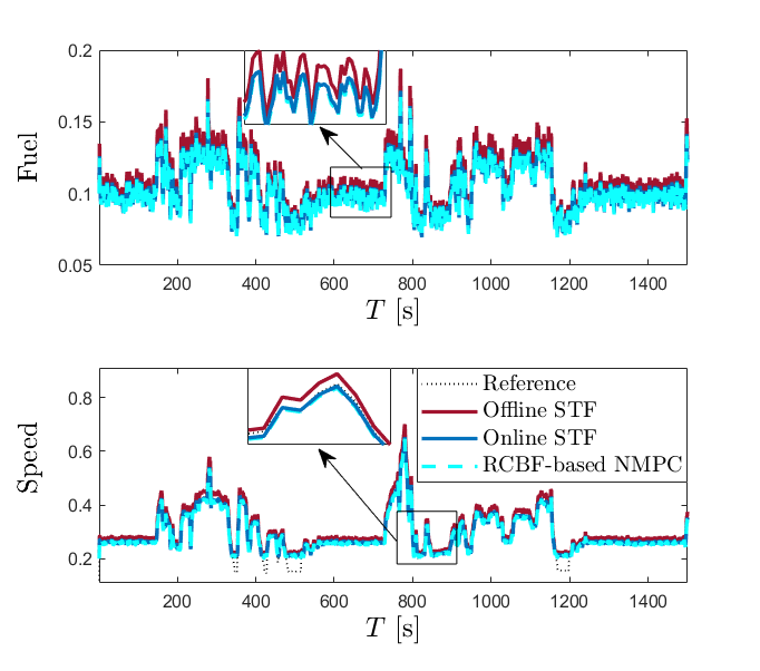
Figure 10: States for engine vehicle using RCBF-based NMPC and data-driven safe predictive control.

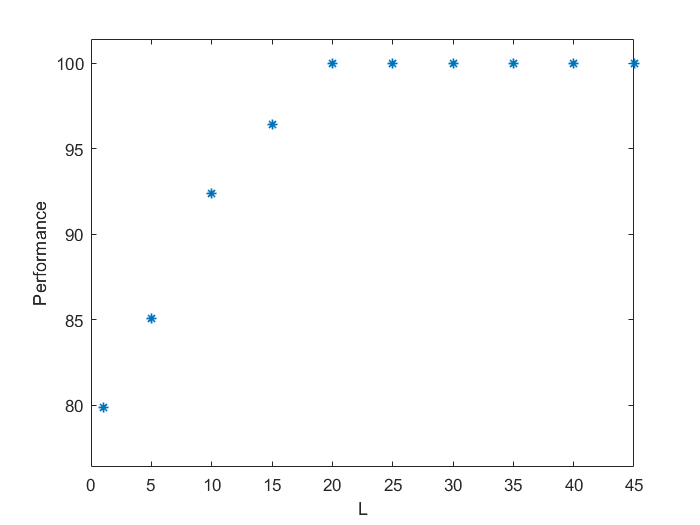
Figure 11: Number of clusters and local models for engine vehicle identification.

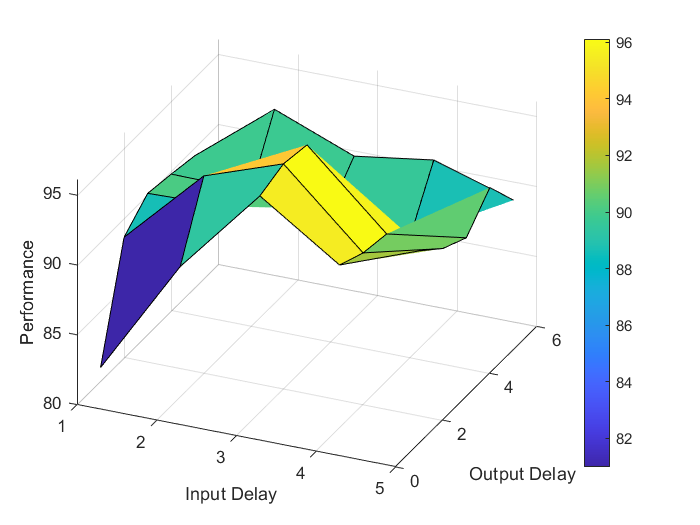
Figure 12: Input delay and output delay for engine vehicle identification.

For the offline part, Table II presents the performance and computational cost of the discrete-time STF-based concurrent learning in comparison with the NNs and the GPR for the engine vehicle identification, and Table III demonstrates the same task for the RCBF-based NMPC policy learning. We evaluate the performance of each function approximator using the best fitting rate (BFR), which analyzes the goodness of fit between the validation data (i.e., measured data) and the simulated output of the trained model (or trained policy) based on the normalized root mean squared error (NRMSE). Thus, the performance represents $(1-\frac{\lVert y-\hat{y}\rVert}{\lVert y-mean(y)\rVert})\times 100\hskip 2.84526pt\%$ and $(1-\frac{\lVert u_{mpc}-\tilde{u}\rVert}{\lVert u_{mpc}-mean(u_{mpc})\rVert})\times 100\hskip 2.84526pt\%$ for Tables II and III, respectively, and 100% performance means that the simulated output from the trained model (or trained policy) is perfectly matched with the measured data. It is worth noting that the measured data for Tables II and III are the collected system output from the engine vehicle and the collected control input from the RCBF-based NMPC, respectively. As shown in Tables II and III, the STF-based concurrent learning effectively reduces the computational cost of the learning process while

TABLE II: Comparison of Performance and Computational Cost for System Identification

Learning	Performance	Time (per loop)
NNs	$96.15\%$	$32.8\hskip 2.84526ptms$
GPR	$96.48\%$	$99.3\hskip 2.84526ptms$
STF	$96.12\%$	$04.3\hskip 2.84526ptms$

TABLE III: Comparison of Performance and Computational Cost for NMPC Policy Learning

Fun. Forms	Performance	Time (per loop)
NNs	$98.12\%$	$19.4\hskip 2.84526ptms$
GPR	$98.57\%$	$58.1\hskip 2.84526ptms$
STF	$98.05\%$	$03.5\hskip 2.84526ptms$

TABLE IV: Comparison of Performance and Computational Cost for Different Controllers

Control	Performance	Time (per loop)
NMPC (N=1)	$98.76\%$	$05.7\hskip 2.84526ptms$
NMPC (N=4)	$99.23\%$	$25.2\hskip 2.84526ptms$
NMPC (N=8)	$99.86\%$	$68.1\hskip 2.84526ptms$
Online STF (N=1)	$98.66\%$	$66.2\hskip 2.84526pt\mu s$
Online STF (N=4)	$99.15\%$	$78.9\hskip 2.84526pt\mu s$
Online STF (N=8)	$99.79\%$	$90.8\hskip 2.84526pt\mu s$

it shows high performance for system identification and NMPC learning compared to the NNs and the GPR. Moreover, for the online part, the online data-driven safe predictive control is compared with the RCBF-based NMPC for various future predictions $N$ in Table IV. This table demonstrates the performance of each controller using the NRMSE between the desired reference trajectory and the simulated system output (using the trained model). Thus, the performance represents $(1-\frac{\lVert r-\hat{y}\rVert}{\lVert r-mean(r)\rVert})\times 100\hskip 2.84526pt\%$, and 100% performance means that the simulated system output is perfectly matched with the desired reference trajectory. One can see that the online data-driven safe predictive control provides high performance to track the desired reference trajectory while it effectively reduces the computational cost of the NMPC.

V Conclusions

In this paper, we developed a unified online data-driven predictive control framework with robust safety guarantees, which includes a discrete-time STF-based concurrent learning for efficient nonlinear system identification with relaxed PE conditions, a RCBF-based NMPC policy approximator to explicitly deal with control learning error, system identification error, and unknown disturbances, and an online adaptation law based on KKT sensitivity analysis and feedback control. The framework was applied to the cart-inverted pendulum as well as an automotive engine with promising results demonstrated. The main contribution of this paper is mainly on the proposed new framework with control law derivations and analysis. The main purpose of the simulation is to demonstrate the effectiveness of the proposed framework by showing that the developed online data-driven safe predictive control is able to achieve a reasonable performance with negligible online computation as compared to the NMPC. The considered cart-inverted pendulum is a classical system frequently used for nonlinear control benchmarks. Moreover, for the second example of simulation part, we have experimentally collected input/output (I/O) data from a turbocharged internal combustion engine and identified a nominal model for the system using the collected data. The proposed data-driven control is applied on the obtained identified model and demonstrates a reasonable performance as shown in the simulation results. We acknowledge a few limitations of our method as follows. Like the NNs and the GPR, the STF framework requires comprehensive data collection to ensure an adequate coverage of operating conditions. Moreover, in the control design, a bounded external disturbance is assumed, and we will extend this framework with more general unbounded stochastic disturbances in our future work. Another assumption we make is on the recursive feasibility of the optimization problem with control input and safety constraints to guarantee the closed-loop performance. Future work will include addressing the mentioned shortcomings by exploring a finite sample approach to reduce the required collected data for the STF and carrying out a formal discussion on the recursive feasibility of the optimization problem, e.g., with an iteration approach. Finally, applications to real-world nonlinear and complex systems such as robots and autonomous vehicles will be performed.

Appendix A (Transferring STF Model to State-Space Model)

Considering (14)-(LABEL:local_models), the input vector of the STF function approximator, i.e., ${U}_{stf}(k+1)$, can be written in the format of $[u(k);x(k)]$ as

$${f}_{i}(k+1)={A}_{i}{U}_{stf}(k+1)+{b}_{i}+\omega_{i}(k+1)$$ (64)

$$\hskip 38.41121pt=A_{i_{2}}x(k)+{A}_{i_{1}}u(k)+{b}_{i}+\omega_{i}(k+1),$$

where ${A}_{i_{1}}$ is the first element of ${A}_{i}$, and $A_{i_{2}}$ represents the rest of the elements, i.e.,

$${A}_{i}=[a_{i_{1}},a_{i_{2}},a_{i_{3}},\ldots,a_{i_{d_{u}+d_{y}}}],$$ (65)

$$A_{i_{1}}=a_{i_{1}},{A}_{i_{2}}=[a_{i_{2}},a_{i_{3}},\ldots,a_{i_{d_{u}+d_{y}}}],$$

$$x(k)=[u(k-1);\ldots;u(k-d_{u}+1);y(k);\ldots;y(k-d_{y}+1)].$$

where $x(k)$ is considered as the states of the system, and $u(k)$ represents the control input.

Now, the nonlinear model (15) is rewritten as

$$y(k+1)=\sum\limits_{i=1}^{L}{\alpha}_{i}(k+1)(A_{i_{2}}x(k)+{A}_{i_{1}}u(k)+{b}_{i}+\omega_{i}(k+1)),$$ (66)

where ${\alpha}_{i}(k+1)$ represents ${\alpha}_{i}([u(k);x(k)],{\psi}_{i})$.

Using (LABEL:parameters_state) and (66), the state-space model (1) is obtained in the following form:

$$x(k+1)=f(x(k),u(k))+w(k),$$ (67)

$$\hskip 36.98857pt=A_{t_{2}}(k)x(k)+{A}_{t_{1}}(k)u(k)+{b}_{t}(k)+w(k),$$

where $A_{t_{2}}$, ${A}_{t_{1}}$, and ${b}_{t}$ are nonlinear matrices as

$$A_{t_{2}}(k)=\begin{bmatrix}0_{n_{u}\times n_{u}(d_{u}-1)}&0_{n_{u}\times n_{y}(d_{y})}\\ \tau_{1}&0_{n_{u}(d_{u}-2)\times n_{y}(d_{y})}\\ \rho_{1}(k)&\rho_{2}(k)\\ 0_{n_{y}(d_{y}-1)\times n_{u}(d_{u}-1)}&\tau_{2}\end{bmatrix},$$ (68)

$$A_{t_{1}}(k)=\begin{bmatrix}I_{n_{u}}\\ 0_{n_{u}(d_{u}-2)\times n_{u}}\\ \sum\limits_{i=1}^{L}{\alpha}_{i}([u(k);x(k)],{\psi}_{i}){A}_{i_{1}},\\ 0_{n_{y}(d_{y}-1)\times n_{u}}\end{bmatrix},$$

$$b_{t}(k)=\begin{bmatrix}0_{n_{u}\times 1}\\ 0_{n_{u}(d_{u}-2)\times 1}\\ \sum\limits_{i=1}^{L}{\alpha}_{i}([u(k);x(k)],{\psi}_{i})b_{i},\\ 0_{n_{y}(d_{y}-1)\times 1}\end{bmatrix},$$

$$w(k)=\begin{bmatrix}0_{n_{u}\times 1}\\ 0_{n_{u}(d_{u}-2)\times 1}\\ \sum\limits_{i=1}^{L}{\alpha}_{i}([u(k);x(k)],{\psi}_{i})\omega_{i}(k+1),\\ 0_{n_{y}(d_{y}-1)\times 1}\end{bmatrix},$$

where

$$\tau_{1}=[I_{n_{u}(d_{u}-2)}\hskip 14.22636pt0_{n_{u}(d_{u}-2)\times n_{u}}],$$ (69)

$$\tau_{2}=[I_{n_{y}(d_{y}-1)}\hskip 14.22636pt0_{n_{y}(d_{y}-1)\times n_{y}}],$$

$$\rho_{1}(k)=\sum\limits_{i=1}^{L}{\alpha}_{i}([u(k);x(k)],{\psi}_{i})[a_{i_{2}},\ldots,a_{i_{d_{u}}}],$$

$$\rho_{2}(k)=\sum\limits_{i=1}^{L}{\alpha}_{i}([u(k);x(k)],{\psi}_{i})[a_{i_{d_{u}+1}},\ldots,a_{i_{d_{u}+d_{y}}}].$$

References

- [1] R. A. Zidek, I. V. Kolmanovsky, and A. Bemporad, “Model predictive control for drift counteraction of stochastic constrained linear systems,” Automatica, vol. 123, p. 109304, 2021.
- [2] C. A. Alonso, J. S. Li, N. Matni, and J. Anderson, “Robust distributed and localized model predictive control,” arXiv preprint arXiv:2103.14171, 2021.
- [3] B. T. Lopez, J.-J. E. Slotine, and J. P. How, “Dynamic tube mpc for nonlinear systems,” in 2019 American Control Conference (ACC), pp. 1655–1662, IEEE, 2019.
- [4] M. Wytock, N. Moehle, and S. Boyd, “Dynamic energy management with scenario-based robust mpc,” in 2017 American Control Conference (ACC), pp. 2042–2047, IEEE, 2017.
- [5] A. Vahidi-Moghaddam, K. Zhang, Z. Li, X. Yin, Z. Song, and Y. Wang, “Extended neighboring extremal optimal control with state and preview perturbations,” arXiv preprint arXiv:2306.04830, 2023.
- [6] A. Vahidi-Moghaddam, Z. Li, N. Li, K. Zhang, and Y. Wang, “Event-triggered cloud-based nonlinear model predictive control with neighboring extremal adaptations,” in 2022 IEEE 61st Conference on Decision and Control (CDC), pp. 3724–3731, IEEE, 2022.
- [7] F. Yazdandoost, H. Razavi, and A. Izadi, “Optimization of agricultural patterns based on virtual water considerations through integrated water resources management modeling,” International Journal of River Basin Management, vol. 20, no. 2, pp. 255–263, 2022.
- [8] M. R. Hajidavalloo, A. Gupta, Z. Li, and W.-C. Tai, “MPC-based vibration control and energy harvesting using stochastic linearization for a new energy harvesting shock absorber,” in 2021 IEEE Conference on Control Technology and Applications (CCTA), pp. 38–43, IEEE, 2021.
- [9] K. Chen, Z. Li, D. Filev, Y. Wang, K. Wu, and J. Wang, “Online nonlinear dynamic system identification with evolving spatial-temporal filters: Case study on turbocharged engine modeling,” IEEE Transactions on Control Systems Technology, vol. 29, no. 3, pp. 1364–1371, 2020.
- [10] S. Akbari, P. H. Dabaghian, and O. San, “Blending machine learning and sequential data assimilation over latent spaces for surrogate modeling of boussinesq systems,” Physica D: Nonlinear Phenomena, vol. 448, p. 133711, 2023.
- [11] A. Ahmadi, M. Talaei, M. Sadipour, A. M. Amani, and M. Jalili, “Deep federated learning-based privacy-preserving wind power forecasting,” IEEE Access, vol. 11, pp. 39521–39530, 2022.
- [12] S. Akbari, S. Pawar, and O. San, “Numerical assessments of a nonintrusive surrogate model based on recurrent neural networks and proper orthogonal decomposition: Rayleigh benard convection,” arXiv preprint arXiv:2212.05384, 2022.
- [13] R. Jamali, G. Battista, M. Martarelli, P. Chiariotti, D. S. Kunte, C. Colangeli, and P. Castellini, “Objective-subjective sound quality correlation performance comparison of genetic algorithm based regression models and neural network based approach,” in Journal of Physics: Conference Series, vol. 2041, p. 012015, IOP Publishing, 2021.
- [14] I. Jebellat, H. N. Pishkenari, and E. Jebellat, “Training microrobots via reinforcement learning and a novel coding method,” in 2021 9th RSI International Conference on Robotics and Mechatronics (ICRoM), pp. 105–111, IEEE, 2021.
- [15] A. Yousefpour, M. Shishehbor, Z. Z. Foumani, and R. Bostanabad, “Unsupervised anomaly detection via nonlinear manifold learning,” arXiv preprint arXiv:2306.09441, 2023.
- [16] Z. Z. Foumani, M. Shishehbor, A. Yousefpour, and R. Bostanabad, “Multi-fidelity cost-aware bayesian optimization,” Computer Methods in Applied Mechanics and Engineering, vol. 407, p. 115937, 2023.
- [17] K. Chen, K. Zhang, Z. Li, Y. Wang, K. Wu, and U. V. Kalabić, “Stochastic model predictive control for quasi-linear parameter varying systems: Case study on automotive engine control,” Journal of Dynamic Systems, Measurement, and Control, vol. 144, no. 6, p. 061005, 2022.
- [18] K. Zhang, Y. Zheng, and Z. Li, “Dimension reduction for efficient data-enabled predictive control,” arXiv preprint arXiv:2211.03697, 2022.
- [19] A. Amiri-Margavi and H. Babaee, “On-the-fly reduced-order modeling of transient flow response subject to high-dimensional external forcing,” Bulletin of the American Physical Society, 2022.
- [20] Y. Zhong, A. Amiri-Margavi, H. Babaee, and K. Taira, “Optimally time-dependent mode analysis of vortex gust-airfoil wake interactions,” Bulletin of the American Physical Society, 2022.
- [21] J. Lore, S. De Pascuale, P. Laiu, B. Phathanapirom, S. Brunton, J. Canik, S. Cetiner, N. Kutz, and P. Stangeby, “Model predictive control of boundary plasmas using reduced models derived from solps-iter,” in APS Division of Plasma Physics Meeting Abstracts, vol. 2021, pp. NM09–002, 2021.
- [22] Y. Bao, K. J. Chan, A. Mesbah, and J. M. Velni, “Learning-based adaptive-scenario-tree model predictive control with probabilistic safety guarantees using bayesian neural networks,” in 2022 American Control Conference (ACC), pp. 3260–3265, IEEE, 2022.
- [23] D. Krishnamoorthy, A. Mesbah, and J. A. Paulson, “An adaptive correction scheme for offset-free asymptotic performance in deep learning-based economic mpc,” IFAC-PapersOnLine, vol. 54, no. 3, pp. 584–589, 2021.
- [24] E. Arcari, M. V. Minniti, A. Scampicchio, A. Carron, F. Farshidian, M. Hutter, and M. N. Zeilinger, “Bayesian multi-task learning mpc for robotic mobile manipulation,” IEEE Robotics and Automation Letters, 2023.
- [25] E. Arcari, A. Carron, and M. N. Zeilinger, “Meta learning mpc using finite-dimensional gaussian process approximations,” arXiv preprint arXiv:2008.05984, 2020.
- [26] S. Dean, A. J. Taylor, R. K. Cosner, B. Recht, and A. D. Ames, “Guaranteeing safety of learned perception modules via measurement-robust control barrier functions,” arXiv preprint arXiv:2010.16001, 2020.
- [27] Y. Chen, J. Anderson, K. Kalsi, A. D. Ames, and S. H. Low, “Safety-critical control synthesis for network systems with control barrier functions and assume-guarantee contracts,” IEEE Transactions on Control of Network Systems, vol. 8, no. 1, pp. 487–499, 2020.
- [28] A. D. Ames, S. Coogan, M. Egerstedt, G. Notomista, K. Sreenath, and P. Tabuada, “Control barrier functions: Theory and applications,” in 2019 18th European control conference (ECC), pp. 3420–3431, IEEE, 2019.
- [29] A. Isaly, B. C. Allen, R. G. Sanfelice, and W. E. Dixon, “Zeroing control barrier functions for safe volitional pedaling in a motorized cycle,” IFAC-PapersOnLine, vol. 53, no. 5, pp. 218–223, 2020.
- [30] S. Shivam, Y. Wardi, M. Egerstedt, A. Kanellopoulos, and K. G. Vamvoudakis, “Intersection-traffic control of autonomous vehicles using newton-raphson flows and barrier functions,” IFAC-PapersOnLine, vol. 53, no. 2, pp. 15733–15738, 2020.
- [31] K. Garg and D. Panagou, “Robust control barrier and control lyapunov functions with fixed-time convergence guarantees,” in 2021 American Control Conference (ACC), pp. 2292–2297, IEEE, 2021.
- [32] M. Black, E. Arabi, and D. Panagou, “A fixed-time stable adaptation law for safety-critical control under parametric uncertainty,” in 2021 European Control Conference (ECC), pp. 1328–1333, IEEE, 2021.
- [33] A. Isaly, O. S. Patil, R. G. Sanfelice, and W. E. Dixon, “Adaptive safety with multiple barrier functions using integral concurrent learning,” in 2021 American Control Conference (ACC), pp. 3719–3724, IEEE, 2021.
- [34] B. T. Lopez, J.-J. E. Slotine, and J. P. How, “Robust adaptive control barrier functions: An adaptive & data-driven approach to safety (extended version),” arXiv preprint arXiv:2003.10028, 2020.
- [35] A. J. Taylor and A. D. Ames, “Adaptive safety with control barrier functions,” in 2020 American Control Conference (ACC), pp. 1399–1405, IEEE, 2020.
- [36] A. Vahidi-Moghaddam, M. Mazouchi, and H. Modares, “Learning dynamics system models with prescribed-performance guarantees using experience-replay,” in 2021 American Control Conference (ACC), pp. 1941–1946, IEEE, 2021.
- [37] A. Vahidi-Moghaddam, M. Mazouchi, and H. Modares, “Memory-augmented system identification with finite-time convergence,” IEEE Control Systems Letters, vol. 5, no. 2, pp. 571–576, 2020.
- [38] G. Chowdhary and E. Johnson, “Concurrent learning for convergence in adaptive control without persistency of excitation,” in 49th IEEE Conference on Decision and Control (CDC), pp. 3674–3679, IEEE, 2010.
- [39] E. W. Bai and S. S. Sastry, “Persistency of excitation, sufficient richness and parameter convergence in discrete time adaptive control,” Systems & control letters, vol. 6, no. 3, pp. 153–163, 1985.
- [40] S. P. H. Boroujeni and E. Pashaei, “A hybrid chimp optimization algorithm and generalized normal distribution algorithm with opposition-based learning strategy for solving data clustering problems,” arXiv preprint arXiv:2302.08623, 2023.
- [41] S. P. H. Boroujeni and E. Pashaei, “Data clustering using chimp optimization algorithm,” in 2021 11th international conference on computer engineering and knowledge (ICCKE), pp. 296–301, IEEE, 2021.
- [42] A. Derakhshan, I. G. Harris, and M. Behzadi, “Detecting telephone-based social engineering attacks using scam signatures,” in Proceedings of the 2021 ACM Workshop on Security and Privacy Analytics, pp. 67–73, 2021.
- [43] G. Chowdhary and E. Johnson, “A singular value maximizing data recording algorithm for concurrent learning,” in Proceedings of the 2011 American Control Conference, pp. 3547–3552, IEEE, 2011.
- [44] A. Vahidi-Moghaddam, K. Chen, Z. Li, Y. Wang, and K. Wu, “Data-driven safe predictive control using spatial temporal filter-based function approximators,” 2022 American Control Conference (ACC), 2022.
- [45] F. Borrelli, A. Bemporad, and M. Morari, Predictive control for linear and hybrid systems. Cambridge University Press, 2017.
- [46] G. Lars and P. Jürgen, “Nonlinear model predictive control theory and algorithms,” 2011.