LISA Dynamics & Control: Closed-loop Simulation and Numerical Demonstration of Time Delay Interferometry

Abstract

The Laser Interferometer Space Antenna (LISA), space-based gravitational wave observatory involves a complex multidimensional closed-loop dynamical system. Its instrument performance is expected to be less efficiently isolated from platform motion than was its simpler technological demonstrator, LISA Pathfinder. It is of crucial importance to understand and model LISA dynamical behavior accurately to understand the propagation of dynamical excitations through the response of the instrument down to the interferometer data streams. More generally, simulation of the system allows for the preparation of the processing and interpretation of in-flight metrology data. In this work, we present a comprehensive mathematical modeling of the closed-loop system dynamics and its numerical implementation within the LISA Consortium simulation suite. We provide, for the first time, a full time-domain numerical demonstration of post-processing Time Delay Interferometer techniques combining multiple position measurements with realistic control loops to create a synthetic Michelson interferometer. We show that in the absence of physical coupling to spacecraft and telescope motion (through tilt-to-length, stiffness and actuation cross-talk) the effect of noisy spacecraft motion is efficiently suppressed to a level below the noise originating in the rest of the instrument.

I Space-based gravitational waves astronomy and LISA detector

The Laser Interferometer Space Antenna (LISA) is a space-based, gravitational wave (GW) observatory planned to launch in 2035 [1]. It aims to open a new window on the Universe in the milliHertz bandwidth of the GW sky, which is expected to harbor a rich and diverse collection of astrophysical and cosmological sources, including the merger events of supermassive black hole binaries [2, 3], believed as among the most energetic events in the observable Universe.

The mission, led by the European Space Agency, consists of three spacecraft arranged in a nearly equilateral triangular constellation, whose barycenter follows the Earth in a heliocentric orbit. Interferometric measurements of the spacecraft separation will be used to measure GW as they pass through the constellation. The scale of the detector and its space environment allow for operation in the millihertz bandwidth. The 2.5 million km arm-lengths result in picometer optical path length variations due to GW, and antenna nulls in the $\displaystyle 40\,$\displaystyle\mathrm{mHz}$$ regime. Operation in space eliminates acoustic, seismic and Newtonian noise disturbances which limit the sensitivity of ground-based detectors below 1 Hz [4].

I.1 Picometer laser interferometry in space

To observe GW with strain amplitudes of order 10^-20, the LISA instrument must overcome two major challenges. Firstly, the satellites are poor references of inertia, being subjected to force noise, from solar wind, solar radiation pressure, and their own micro-propulsion system [5]. To overcome this obstacle, cubic Au-Pt alloy $\displaystyle 1.92\,$\displaystyle\mathrm{kg}$$ test-masses within the spacecraft are used as the end-mirrors of the interferometer. Protected from environmental force noise, they constitute a very good approximation to local inertial reference frames on-board the spacecraft. They are housed in vacuum chambers and surrounded by electrodes which allow for position sensing and actuation [6]. Interferometric sensing is preferred to probe the test-mass displacement relative to their housings along the directions of the arm lengths [7, 8] (cf. constellation and geometry spacecraft in Figure 1 and 2). These test-mass interferometers (TMIs) are exploited to monitor and suppress the spacecraft acceleration in the long-range science interferometers—called inter-spacecraft interferometers (ISIs) [9]. The ability to fly $\displaystyle 1.92\,$\displaystyle\mathrm{kg}$$ cubic references of inertia with stability performance compatible with GW astronomy has been successfully demonstrated by the LISA Pathfinder mission [10, 11, 12].

Secondly, a Michelson-type interferometer with million-km arm-lengths cannot be realized in space without post-processing techniques. Reflected laser roundtrips along the arms are prohibited by the available laser power on-board, and frequency noise suppression by optical path length matching is made impossible as the spacecraft orbital mechanics result in arm-lengths that are mismatched and changing over time. Instead, a collection of heterodyne interferometric measurements between local laser beams and propagated distant laser beams is performed across the constellation [9], and the resulting beat notes are time synchronized on-ground accounting for light propagation time delays, and linearly combined so that the laser noise is suppressed: this post-processing technique is called Time Delay Interferometry (TDI) [13, 14].

Tackling these two technological challenges renders the measurement complex and composite, relying strongly on multiple post-processing steps to produce data exploitable for astronomy. Preparing for the successful operation of the mission, it is therefore crucial to understand, model, and simulate the instrument response and data generation in order to test with a high degree of representativity data interpretation and analysis strategies and methods.

I.2 Metrology on-board

To guarantee the best stability of the apparatus, and precise centering and alignment of the test-masses in their housings, the spacecraft embed high-precision sensor and actuation systems. Local optical Interferometry Systems (IFOs) provide picometer-stable test-mass displacement sensing along the telescope axes (see Figure 2 for the spacecraft geometry). These optical readouts are used as TMI in the overall TDI and contribute to the final interferometer data streams. An alternative combination of the interferometer quadrant photodiode readout signals allows for a high-precision sensing of test-mass angular motion in two degrees of freedom using a method known as Differential Wavefront Sensing (DWS) [8]. The Gravitational Reference System (GRS) provides $\displaystyle\sim$nm and $\displaystyle\sim$100 nRad electrostatic sensing of all test-mass longitudinal and angular displacements, through the measurement of differential capacitance changes on a set of electrodes surrounding the test-mass [6]. This set of capacitors is also used to exert correction forces and torques on the test-masses through audio frequency voltages applied to the electrodes [15]. Control forces on the test-masses are triggered only by their differential motion [16]. The DWS technique is exploited again to sense the angle of the long-range inter-spacecraft laser beam w.r.t. the telescope axes. The magnification of the telescope allows for sub-nanoradian sensing of spacecraft attitude and telescopes: this measurement is referred to as the Long-arm Differential Wavefront Sensing (LDWS). The assembly of the telescope, the optical bench, and the GRS housing the test-masses is named the Moving Optical Sub-Assembly (MOSA). It will rotate about the test-mass axis to allow for the variation in the opening angle of the constellation due to orbital variations known as breathing. Spacecraft longitudinal and attitude control are performed using a system of micronewton thrusters [5], which allows the satellite to track the test-masses in their free-fall (drag-free control), and to lock its attitude on the laser beam received from the distant spacecraft (attitude control). A rotation mechanism is used for slow actuation of the MOSA ensuring the pointing direction tracks the incoming laser beam direction and nulls the LDWS output. The sensing, actuation, and control systems are summarized in Table 1. Noise performance values, which will be considered in the simulation, will be discussed in section V and summarized in Table 2. Performance estimates are based on the current LISA design and measurements from the LISA Pathfinder mission [10, 12, 8].

Table 1: For each control coordinate, the table lists the respective control type and actuator used, as well as the subsystem they are sensed with. Capital letters are used for spacecraft coordinates, while lower case and indices are used for test-mass coordinates. The table is adapted from Table I. of [16], to which the control of the telescopes’ opening angle $\displaystyle\hat{\phi}_{m}$ has been added in row 7.

#	Coord.	Sensor	Control Mode	Actuator	Command
1	$\displaystyle\hat{x}_{\scriptscriptstyle 1}$	IFO	Drag-Free	$\displaystyle\mu$-thrust	$\displaystyle f_{X}^{\text{drag-free}}$
2	$\displaystyle\hat{x}_{\scriptscriptstyle 2}$	IFO	Drag-Free	$\displaystyle\mu$-thrust	$\displaystyle f_{Y}^{\text{drag-free}}$
3	$\displaystyle\hat{z}_{\scriptscriptstyle 1}$	GRS	Drag-Free	$\displaystyle\mu$-thrust	$\displaystyle f_{Z}^{\text{drag-free}}$
4	$\displaystyle\hat{\Theta}$	LDWS	Attitude	$\displaystyle\mu$-thrust	$\displaystyle t_{X}^{\text{att}}$
5	$\displaystyle\hat{H}$	LDWS	Attitude	$\displaystyle\mu$-thrust	$\displaystyle t_{Y}^{\text{att}}$
6	$\displaystyle\hat{\Phi}$	LDWS	Attitude	$\displaystyle\mu$-thrust	$\displaystyle t_{Z}^{\text{att}}$
7	$\displaystyle\hat{\phi}_{m}$	LDWS	Tel. Pointing	MOSA mechanism	$\displaystyle t_{z_{\scriptscriptstyle 1}}^{\text{tel}}$ / $\displaystyle t_{z_{\scriptscriptstyle 2}}^{\text{tel}}$
8	$\displaystyle\hat{y}_{\scriptscriptstyle 1}$	GRS	Suspension	GRS	$\displaystyle f_{y_{1}}^{\text{sus}}$
9	$\displaystyle\hat{y}_{\scriptscriptstyle 2}$	GRS	Suspension	GRS	$\displaystyle f_{y_{2}}^{\text{sus}}$
10	$\displaystyle\hat{z}_{\scriptscriptstyle 2}$	GRS	Suspension	GRS	$\displaystyle f_{z_{1}}^{\text{sus}}$ / $\displaystyle f_{z_{2}}^{\text{sus}}$
11	$\displaystyle\hat{\theta}_{\scriptscriptstyle 1}$	GRS	Suspension	GRS	$\displaystyle t_{x_{1}}^{\text{sus}}$
12	$\displaystyle\hat{\eta}_{\scriptscriptstyle 1}$	IFO	Suspension	GRS	$\displaystyle t_{y_{1}}^{\text{sus}}$
13	$\displaystyle\hat{\phi}_{\scriptscriptstyle 1}$	IFO	Suspension	GRS	$\displaystyle t_{z_{1}}^{\text{sus}}$
14	$\displaystyle\hat{\theta}_{\scriptscriptstyle 2}$	GRS	Suspension	GRS	$\displaystyle t_{x_{2}}^{\text{sus}}$
15	$\displaystyle\hat{\eta}_{\scriptscriptstyle 2}$	IFO	Suspension	GRS	$\displaystyle t_{y_{2}}^{\text{sus}}$
16	$\displaystyle\hat{\phi}_{\scriptscriptstyle 2}$	IFO	Suspension	GRS	$\displaystyle t_{z_{2}}^{\text{sus}}$

I.3 Operating without a direct optical differential channel

A key difference LISA Pathfinder and LISA is that no direct, differential optical measurements between test-masses will be available for LISA, neither locally within the spacecraft, nor at the constellation scale between distant test-masses. Indeed, as will be discussed in more detail in the final section of this work (cf. Figure 7), the long-range optical measurement is split into three pieces: one local test-mass to spacecraft TMI measurement, one long-range ISI measurement, and a second TMI measurement at the other end of the interferometer arm. The necessary decomposition of the long-range interferometers makes the detector performance more liable to spacecraft and telescope dynamical stability than in the LISA Pathfinder case, where test-mass-to-test-mass measurements were by construction efficiently isolated from noisy spacecraft motion. [12, 10]. In particular, optical geometrical misalignment and off-centering will introduce Tilt-To-Length (TTL) coupling to the spacecraft and telescope noisy angular motion [17, 18]. This effect is expected to be one of the leading noise contributors to the overall noise budget of the instrument. In addition, electrostatic and gravitational fields create a force gradient at the test-mass—referred to as stiffnesses—that couples to spacecraft motion and generates acceleration noise.

Dynamical stability plays a driving role in both of these disturbances and is a key property for LISA performance. It is of crucial importance to model the closed-loop dynamics of the spacecraft-telescopes-test-masses system to assess accurately such dynamical noise, and demonstrate our ability to mitigate the impact of dynamical artifacts on LISA data analysis. LISA dynamics modeling has been already addressed in recent literature [19], in the scope of Drag-Free and Attitude Control System (DFACS) design, and implemented in a proprietary software Matlab/Simscape. Here we present an implementation of a full closed-loop dynamics simulation integrated into the python based consortium End-To-End (E2E) simulation suite and dedicated to LISA data processing and analysis. We provide the modeling framework and the Equations Of Motion (EOM) at play in comprehensive detail, as we believe it deserves an elaborated and formalized reference in the scope of future LISA in-flight data diagnostics and interpretation.

I.4 Simulating LISA dynamics

Among the simulation tools developed by the LISA consortium, the LISANode software [20] is particularly well-suited for spacecraft dynamics and control simulation. Its graph-based, modular framework naturally lends itself to control system implementation (in a similar way to commonly-used Matlab-Simulink tools) and its generation and management of time series data, operating on quantities as they flow between graphs, enables long simulations with efficient use of memory [21].

In this paper, the full derivation of the EOM of the LISA dynamical system is developed and its implementation in the LISANode simulation tool is described. This includes implementation of the EOM, simulations of the sensing systems, and implementation of the feedback loop, interface with the interferometer measurements, and post-processing the resulting beat notes with TDI. For the first time, the impact of spacecraft and test-mass dynamics, and control on LISA data at the level of heterodyne beat notes fluctuations and the TDI channels can be studied.

This article is organized as follows: We introduce the LISA dynamical system, describing the relevant reference frames in Section II. Simulation of the EOM for the test-masses and spacecraft are detailed in Section III. These equations are simplified in Section IV by linearizing around a stable working point, which is maintained by the controllers detailed in Section V. Numerical solving methods used for the linear system approximation, as well as the full non-linear dynamical system, are detailed in Section VI. Results of the dynamics simulations are shown in Section VII, and in particular a demonstration of jitter suppression in Section VIII.

II Dynamical system and Reference Frames

This section is dedicated to the full derivation of LISA EOMs and their insertion into the closed-loop system, including sensors and actuators. The EOM are indeed a core piece of the simulation and deserve thorough attention. A preliminary step is the definition of the dynamical coordinates and reference frames necessary to describe fully the dynamical state of the system. We based our mathematical modeling on a rigid-body approximation in which the dynamical state of a body is described by the motion of its center of mass (CoM) and its angular velocity w.r.t. an inertial frame: $\displaystyle\left\{\overrightarrow{{\bf\it r}}_{\scriptscriptstyle\text{body}},\overrightarrow{{\bf\it\omega}}_{\scriptscriptstyle\text{body}/\text{gal.}}\right\}$. Each LISA spacecraft is a 20 Degree of Freedom (DoF) system, six for each of the spacecraft and test-mass translational and rotational dynamics, and an additional two for the MOSAs that will rotate along with the constellation orbital breathing. The remaining MOSA DoFs are assumed rigidly fixed to the spacecraft. We note that in nominal operations, MOSA angle actuation is designed to be symmetric, hence suppressing one DoF. However, other modes of operation where this rotation is asymmetric are possible, so it is preferable at this stage to maintain generality.

The LISA dynamics will be operated in closed-loop control by the onboard DFACS, locking the test-mass and spacecraft DoFs onto specific target points as described in Section V. To simulate the system, it is therefore required to express the dynamics of the system in the frame of reference from which they are observed. For example, the test-mass dynamics need to be expressed in the frame attached to its housing they are lodged in, since it is, to first approximation, the reference for the GRS and IFO sensing. This requirement results in the presence of several imbricated, non-inertial reference frames, which, when coupled with the multidimensionality of the system increases the complexity of its description. As a first step, we list and define the set of reference frames we use in the simulation, after which we will select a state representation of the dynamics which facilitates mapping of sensing and actuation.

II.1 Frames of reference

The dynamical model invokes six different types of reference frame—each with its own system of coordinates. One reference frame per rotating, rigid body (spacecraft, test-mass, MOSA) will be used to describe relative orientation between bodies. Two frames associated with the fiducial rotation of the spacecraft and MOSA about their operation point, that facilitate linearization (as discussed in Section IV) and one inertial reference frame. These frames are defined as follows:

• Galilean (inertial) $\displaystyle\mathcal{J}$-frame, fixed w.r.t. distant stars, and with orientation defined according to the International Celestial Reference System (ICRS) convention [22].

• The $\displaystyle\mathcal{O}$-frames (or $\displaystyle\mathcal{B^{*}}$-frames) which set the target attitude for the spacecraft. It is built following the diagram in Figure 1:

  • $\displaystyle x$-axis $\displaystyle\hat{\mathbf{e}}_{x,\mathcal{O}_{\scriptscriptstyle i}}$ is constructed as the bisector of constellation, through local summit spacecraft.

  • $\displaystyle z$-axis $\displaystyle\hat{\mathbf{e}}_{z,\mathcal{O}_{\scriptscriptstyle i}}$ is the unit vector normal to the constellation plane.

  • $\displaystyle y$-axis $\displaystyle\hat{\mathbf{e}}_{y,\mathcal{O}_{\scriptscriptstyle i}}$ is built from the cross product of the two above.

  • The origin $\displaystyle O_{i}$ of the frame $\displaystyle\mathcal{O}_{i}$ follows the ideal orbit of the spacecraft.

• The $\displaystyle\mathcal{B}$-frames rigidly attached to the spacecraft and describing its attitude, whether w.r.t to $\displaystyle\mathcal{O}$-frame or $\displaystyle\mathcal{J}$-frame:

  • $\displaystyle x$-axis $\displaystyle\hat{\mathbf{e}}_{x,\mathcal{B}_{i}}$ is constructed as the bisector to the angle between the two MOSAs axes of spacecraft $\displaystyle i$.

  • $\displaystyle z$-axis $\displaystyle\hat{\mathbf{e}}_{z,\mathcal{B}_{i}}$ is the unit vector normal to the solar panel plane (defining the $\displaystyle xOy$ plane).

  • $\displaystyle y$-axis $\displaystyle\hat{\mathbf{e}}_{y,\mathcal{B}_{i}}$ is deduced from the two above.

  • The origin $\displaystyle B_{i}$ of the frame $\displaystyle\mathcal{B}_{i}$ are the centers of mass of the spacecraft.

• The $\displaystyle\mathcal{H^{*}}$-frames define the target attitude of the MOSA s w.r.t to $\displaystyle\mathcal{J}$-frame.

  • $\displaystyle x$-axis $\displaystyle\hat{\mathbf{e}}_{x,\mathcal{H}^{*}_{j}}$ is the unit vector aligned to the axis normal to the incoming wavefront as intercepted by the telescope $\displaystyle j=(1,2)$ of the local spacecraft $\displaystyle i$. It can be deduced from a rotation of the unit vector $\displaystyle\hat{\mathbf{e}}_{x,\mathcal{O}_{\scriptscriptstyle i}}$ around $\displaystyle\hat{\mathbf{e}}_{z,\mathcal{O}_{\scriptscriptstyle i}}$ of an angle $\displaystyle[-1]^{\scriptscriptstyle j+1}\ \tfrac{\phi_{m}^{*}}{2}$ equal to half the constellation’s opening angle at local spacecraft $\displaystyle i$ location.

  • $\displaystyle z$-axis $\displaystyle\hat{\mathbf{e}}_{z,\mathcal{H}^{*}_{j}}$ is the unit vector normal to LISA constellation plane. It is equal to $\displaystyle\hat{\mathbf{e}}_{z,\mathcal{O}_{\scriptscriptstyle i}}$.

  • $\displaystyle y$-axis $\displaystyle\hat{\mathbf{e}}_{y,\mathcal{H}^{*}_{j}}$ is deduced from the two above.

  • The origin $\displaystyle H_{j}$ of the frame $\displaystyle\mathcal{H}_{j}$ is the geometrical center of the housing $\displaystyle j$ of the spacecraft $\displaystyle i$.

• The $\displaystyle\mathcal{H}$-frames are rigidly attached to their respective MOSA and define their actual attitude, whether w.r.t to $\displaystyle\mathcal{H}^{*}$-frame, $\displaystyle\mathcal{B}$-frame, $\displaystyle\mathcal{O}$-frame or $\displaystyle\mathcal{J}$-frame.

  • $\displaystyle x$-axis $\displaystyle\hat{\mathbf{e}}_{x,\mathcal{H}_{j}}$ is the axis along which local OMS measurement of spacecraft to test-mass $\displaystyle j=(1,2)$ is performed. It is a drag-free axis. It can be deduced from a rotation of the unit vector $\displaystyle\hat{\mathbf{e}}_{x,\mathcal{B}_{\scriptscriptstyle i}}$ around $\displaystyle\hat{\mathbf{e}}_{z,\mathcal{B}_{\scriptscriptstyle i}}$ of an angle $\displaystyle[-1]^{\scriptscriptstyle j+1}\ \tfrac{\phi_{m}}{2}$ equal to half the MOSA’s opening angle of the spacecraft $\displaystyle i$.

  • $\displaystyle z$-axis $\displaystyle\hat{\mathbf{e}}_{z,\mathcal{H}_{j}}$ is the unit vector normal to the solar panel plane (defining the $\displaystyle(xOy)$ plane). It is equal to $\displaystyle\hat{\mathbf{e}}_{z,\mathcal{B}_{i}}$ in the simulator.

  • $\displaystyle y$-axis $\displaystyle\hat{\mathbf{e}}_{y,\mathcal{H}_{j}}$ is deduced from the two above.

  • The origin $\displaystyle H_{j}$ of the frame $\displaystyle\mathcal{H}_{j}$ is the geometrical center of the housing $\displaystyle j$ of the spacecraft $\displaystyle i$.

  • The pivot points $\displaystyle P_{j}$ denote the center of rotation of the MOSA $\displaystyle j$ in the satellite $\displaystyle i$, and coincide with $\displaystyle H_{j}$ in the nominal, geometrical configuration.

• The $\displaystyle\mathcal{T}$-frames are rigidly attached to the corresponding test-masses and describe their attitude, whether w.r.t to $\displaystyle\mathcal{H}$-frame, $\displaystyle\mathcal{B}$-frame, $\displaystyle\mathcal{O}$-frame or $\displaystyle\mathcal{J}$-frame:

  • $\displaystyle x$-axis $\displaystyle\hat{\mathbf{e}}_{x,\mathcal{T}_{j}}$ is constructed as the unit vector normal the $\displaystyle x$-faces of the Test Mass (TM) $\displaystyle j$ and aligned with $\displaystyle\hat{\mathbf{e}}_{x,\mathcal{H}_{j}}$ when nominally oriented.

  • $\displaystyle z$-axis $\displaystyle\hat{\mathbf{e}}_{z,\mathcal{T}_{j}}$ is constructed as a unit vector normal to the $\displaystyle z$-faces of the TM $\displaystyle j$ and aligned with $\displaystyle\hat{\mathbf{e}}_{z,\mathcal{H}_{j}}$ when nominally oriented.

  • $\displaystyle y$-axis $\displaystyle\hat{\mathbf{e}}_{y,\mathcal{T}_{j}}$ is deduced from the two above.

  • The origin $\displaystyle T_{j}$ of the frame $\displaystyle\mathcal{T}_{j}$ is the center of mass of the test-mass $\displaystyle j$.

Figure 1: Figure cut of constellation geometry in the triangle plane. The geometrical construction of the $\displaystyle\mathcal{O}_{1}$ is illustrated. The satellite positions considered in order to build the $\displaystyle\mathcal{O}$-frames are computed from the macroscopic orbital motions only, that is, neglecting the (dynamical state-dependent) stray forces inducing spacecraft jitter. However, state-independent dc forces deviating the spacecraft from pure free-fall can be accounted for in the definition of $\displaystyle\mathcal{O}$-frames.

Figure 2: Figure cut of spacecraft geometry on the $\displaystyle xOy$ plane of the spacecraft body frame $\displaystyle\mathcal{B}$. The reference frames attached to the spacecraft, the housings and the test-masses, resp. $\displaystyle\mathcal{B}$, $\displaystyle\mathcal{H}$ and $\displaystyle\mathcal{T}$, are drawn. Short notation has been preferred for readability to label the axes and coordinates associated to these frames, as explained in section II.3, Equations (28), (29), (32) and (33).

We finally mention the important mathematical relationship in Equation (1), which will be used throughout the document: the so-called transport equation, sometimes called the Varignon formula, named after the late 17th century french mathematician Pierre Varignon. It relates time-derivatives of a given vector w.r.t. to different reference frames (here $\displaystyle\mathcal{B}$ and $\displaystyle\mathcal{J}$)

$$\derivative{t}\Bigg{|}_{\scriptscriptstyle\mathcal{\mathcal{J}}}\mspace{-10.0mu}\left[\ -\ \right]=\derivative{t}\Bigg{|}_{\scriptscriptstyle\mathcal{\mathcal{B}}}\mspace{-10.0mu}\left[\ -\ \right]+\overrightarrow{{\bf\it\omega}}_{\scriptscriptstyle\mathcal{B}/\mathcal{J}}\times\left[\ -\ \right]\ .$$ (1)

II.2 Geometrical construction of target frames

While $\displaystyle\mathcal{J}$, $\displaystyle\mathcal{B}$, $\displaystyle\mathcal{H}$ and $\displaystyle\mathcal{T}$ reference frames are self-defining as each of them rely on existing bodies (distant stars, spacecraft, MOSA s and test-masses), the targeted frames $\displaystyle\mathcal{O}$ and $\displaystyle\mathcal{H}^{*}$ required a physical definition to be utilized as coordinate systems in LISA EOM. Their objective is to encode the nominal orientation of the spacecraft and the MOSA s w.r.t. the Galilean frame $\displaystyle\mathcal{J}$. They are formed using idealized bodies, that is, from the trajectory the spacecraft would follow if they were subject to solar system gravitational field only, hence freely following their respective geodesics. Indeed, given the dimension of the LISA constellation compared to spacecraft dimension and noisy deviation from geodesics, target frames can reliably be constructed from orbits in a very solid approximation (hence neglecting in their definition the microscopic local jittering from geodesics).

As stated in section II.1, $\displaystyle\mathcal{O}$ frame $\displaystyle X$-axis is defined as the bisector of the constellation from the spacecraft $\displaystyle i$ at study. The bisector vector, $\displaystyle\vv{\mathbf{O}_{\scriptscriptstyle i}\mathbf{I}_{\scriptscriptstyle i}}$, for spacecraft $\displaystyle i$ is then

$$\begin{split}\vv{\mathbf{O}_{\scriptscriptstyle i}\mathbf{I}_{\scriptscriptstyle i}}=\overrightarrow{{\bf\it r}}_{\scriptscriptstyle ij}+\left[\frac{r_{ij}}{r_{ij}+r_{ik}}\right]\overrightarrow{{\bf\it r}}_{\scriptscriptstyle jk}=\overrightarrow{{\bf\it r}}_{\scriptscriptstyle ij}+u_{i}\overrightarrow{{\bf\it r}}_{\scriptscriptstyle jk}\ ,\end{split}$$ (2)

using the angle bisector theorem, and where $\displaystyle\overrightarrow{{\bf\it r}}_{\scriptscriptstyle ij}$ is the relative position between two of the three spacecraft (see Equation (3)), which are labeled with $\displaystyle\{i,j,k\}$ letters triplet, $\displaystyle i$ denoting the local spacecraft, $\displaystyle j$ the distant spacecraft facing TM $\displaystyle 1$ of spacecraft $\displaystyle i$, and $\displaystyle k$ facing its TM $\displaystyle 2$ (cf. Figure 1).

$$\overrightarrow{{\bf\it r}}_{\scriptscriptstyle ij}=\overrightarrow{{\bf\it r}}_{\scriptscriptstyle j}-\overrightarrow{{\bf\it r}}_{\scriptscriptstyle i}=\overrightarrow{{\bf\it r}}_{\scriptscriptstyle O_{\scriptscriptstyle j}/J}-\overrightarrow{{\bf\it r}}_{\scriptscriptstyle O_{\scriptscriptstyle i}/J}\ .$$ (3)

Therefore, the $\displaystyle\hat{\mathbf{e}}_{x,\mathcal{O}_{\scriptscriptstyle i}}$ basis vector is defined as

$$\hat{\mathbf{e}}_{x,\mathcal{O}_{\scriptscriptstyle i}}=\frac{\vv{\mathbf{O}_{\scriptscriptstyle i}\mathbf{I}_{\scriptscriptstyle i}}}{\norm{\vv{\mathbf{O}_{\scriptscriptstyle i}\mathbf{I}_{\scriptscriptstyle i}}}}\ .$$ (4)

Finally, the $\displaystyle\hat{\mathbf{e}}_{y,\mathcal{O}_{\scriptscriptstyle i}}$ and $\displaystyle\hat{\mathbf{e}}_{z,\mathcal{O}_{\scriptscriptstyle i}}$ basis vectors are determined by

$$\displaystyle\hat{\mathbf{e}}_{z,\mathcal{O}_{\scriptscriptstyle i}}=\frac{\vv{\mathbf{O}_{\scriptscriptstyle i}\mathbf{I}_{\scriptscriptstyle i}}\times\overrightarrow{{\bf\it r}}_{\scriptscriptstyle jk}}{\norm{\vv{\mathbf{O}_{\scriptscriptstyle i}\mathbf{I}_{\scriptscriptstyle i}}\times\overrightarrow{{\bf\it r}}_{\scriptscriptstyle jk}}}\ ,$$ (5)

$$\displaystyle\hat{\mathbf{e}}_{y,\mathcal{O}_{\scriptscriptstyle i}}=\hat{\mathbf{e}}_{z,\mathcal{O}_{\scriptscriptstyle i}}\times\hat{\mathbf{e}}_{x,\mathcal{O}_{\scriptscriptstyle i}}\ .$$ (6)

The basis vectors of the $\displaystyle\mathcal{O}$ frame are now completely defined from orbital position data $\displaystyle\overrightarrow{{\bf\it r}}_{\scriptscriptstyle i}$, $\displaystyle\overrightarrow{{\bf\it r}}_{\scriptscriptstyle j}$, and $\displaystyle\overrightarrow{{\bf\it r}}_{\scriptscriptstyle k}$. The dynamics of this frame—that is, angular velocity and acceleration—relatively to the Galilean frame $\displaystyle\mathcal{J}$ will come into play when deriving LISA EOM. To avoid numerical difficulties arising from the differentiation of orbits necessary to compute these angular quantities, we should derive them purely symbolically from orbital positions, velocities and accelerations w.r.t. $\displaystyle\mathcal{J}$-frame.

Indeed, angular velocity can be related to the rate of changes of basis vector (mathematical proof in appendix A) from the following expression

$$\displaystyle\begin{split}\overrightarrow{{\bf\it\omega}}_{\scriptscriptstyle\mathcal{O}_{\scriptscriptstyle i}/\mathcal{J}}=\ &\frac{1}{2}\ \hat{\mathbf{e}}_{x,\mathcal{O}_{\scriptscriptstyle i}}\times\derivative{t}\Bigg{|}_{\scriptscriptstyle\mathcal{J}}\mspace{-10.0mu}\left[\hat{\mathbf{e}}_{x,\mathcal{O}_{\scriptscriptstyle i}}\right]\\ &+\frac{1}{2}\ \hat{\mathbf{e}}_{y,\mathcal{O}_{\scriptscriptstyle i}}\times\derivative{t}\Bigg{|}_{\scriptscriptstyle\mathcal{J}}\mspace{-10.0mu}\left[\hat{\mathbf{e}}_{y,\mathcal{O}_{\scriptscriptstyle i}}\right]\\ &+\frac{1}{2}\ \hat{\mathbf{e}}_{z,\mathcal{O}_{\scriptscriptstyle i}}\times\derivative{t}\Bigg{|}_{\scriptscriptstyle\mathcal{J}}\mspace{-10.0mu}\left[\hat{\mathbf{e}}_{z,\mathcal{O}_{\scriptscriptstyle i}}\right]\ ,\end{split}$$ (7)

which then implies an analytical differentiation of expressions (4), (6) and (5) w.r.t. time. These basis vectors being functions $\displaystyle\overrightarrow{\mathbf{f}}$ of orbital elements only—that is $\displaystyle\hat{\mathbf{e}}_{x,\mathcal{O}_{\scriptscriptstyle i}}=\overrightarrow{\mathbf{f}}_{e_{x}}(\overrightarrow{{\bf\it r}}_{\scriptscriptstyle i},\overrightarrow{{\bf\it r}}_{\scriptscriptstyle j},\overrightarrow{{\bf\it r}}_{\scriptscriptstyle k})$ taking the $\displaystyle X$-axis of $\displaystyle\mathcal{O}$-frame as example—it is clear that the angular velocity and acceleration can also be written as mere functions $\displaystyle\overrightarrow{\mathbf{f}}$ of orbital positions, velocities and accelerations, respectively $\displaystyle\overrightarrow{{\bf\it\omega}}_{\scriptscriptstyle\mathcal{O}_{\scriptscriptstyle i}/\mathcal{J}}=\overrightarrow{\mathbf{f}}_{\omega}(\overrightarrow{{\bf\it r}}_{\scriptscriptstyle i,j,k},\overrightarrow{{\bf\it v}}_{\scriptscriptstyle i,j,k})$ and $\displaystyle\derivative{t}\Bigg{|}_{\scriptscriptstyle\mathcal{J}}\mspace{-10.0mu}\left[\overrightarrow{{\bf\it\omega}}_{\scriptscriptstyle\mathcal{O}_{\scriptscriptstyle i}/\mathcal{J}}\right]=\overrightarrow{\mathbf{f}}_{\dot{\omega}}(\overrightarrow{{\bf\it r}}_{\scriptscriptstyle i,j,k},\overrightarrow{{\bf\it v}}_{\scriptscriptstyle i,j,k},\overrightarrow{{\bf\it w}}_{\scriptscriptstyle i,j,k})$. Starting with differentiation of Equation (4), we have

$$\begin{split}\derivative{t}\Bigg{|}_{\scriptscriptstyle\mathcal{J}}\mspace{-10.0mu}\left[\hat{\mathbf{e}}_{x,\mathcal{O}_{\scriptscriptstyle i}}\right]=\frac{\text{O}_{\scriptscriptstyle i}\text{I}_{\scriptscriptstyle i}\derivative{\vv{\mathbf{O}_{\scriptscriptstyle i}\mathbf{I}_{\scriptscriptstyle i}}{}}{t}-\derivative{\text{O}_{\scriptscriptstyle i}\text{I}_{\scriptscriptstyle i}}{t}\vv{\mathbf{O}_{\scriptscriptstyle i}\mathbf{I}_{\scriptscriptstyle i}}}{\text{O}_{\scriptscriptstyle i}\text{I}_{\scriptscriptstyle i}^{2}}\end{split}$$ (8)

from which one can find its contribution to $\displaystyle\overrightarrow{\mathbf{f}}_{\omega}(\overrightarrow{{\bf\it r}}_{\scriptscriptstyle i,j,k},\overrightarrow{{\bf\it v}}_{\scriptscriptstyle i,j,k})$ in expanding Equation (8) using

$$\displaystyle\text{O}_{\scriptscriptstyle i}\text{I}_{\scriptscriptstyle i}=\sqrt{(\overrightarrow{{\bf\it r}}_{\scriptscriptstyle ij}+u_{i}\overrightarrow{{\bf\it r}}_{\scriptscriptstyle jk})\cdot(\overrightarrow{{\bf\it r}}_{\scriptscriptstyle ij}+u_{i}\overrightarrow{{\bf\it r}}_{\scriptscriptstyle jk})}\ ,$$ (9)

$$\displaystyle\derivative{\vv{\mathbf{O}_{\scriptscriptstyle i}\mathbf{I}_{\scriptscriptstyle i}}}{t}=\overrightarrow{{\bf\it v}}_{\scriptscriptstyle ij}+{\dot{u}_{i}}\overrightarrow{{\bf\it r}}_{\scriptscriptstyle jk}+u_{i}\overrightarrow{{\bf\it v}}_{\scriptscriptstyle jk}\ ,$$ (10)

$$\displaystyle\derivative{\text{O}_{\scriptscriptstyle i}\text{I}_{\scriptscriptstyle i}}{t}=\derivative{\vv{\mathbf{O}_{\scriptscriptstyle i}\mathbf{I}_{\scriptscriptstyle i}}}{t}\cdot\hat{\mathbf{e}}_{x,\mathcal{O}_{\scriptscriptstyle i}}\ ,$$ (11)

$$\displaystyle{\dot{u}_{i}}=\frac{(r_{ik}+r_{ij})\dot{r}_{ij}-r_{ij}(\dot{r}_{ij}+\dot{r}_{ik})}{(r_{ij}+r_{ik})^{2}}\ ,$$ (12)

$$\displaystyle r_{ij}=\sqrt{\overrightarrow{{\bf\it r}}_{\scriptscriptstyle ij}\cdot\overrightarrow{{\bf\it r}}_{\scriptscriptstyle ij}}\ ,\hskip 28.45274pt\dot{r}_{ij}=\frac{\overrightarrow{{\bf\it v}}_{\scriptscriptstyle ij}\cdot\overrightarrow{{\bf\it r}}_{\scriptscriptstyle ij}}{r_{ij}}\ .$$ (13)

Now treating the $\displaystyle Z$-axis, we define the following intermediate vectorial and scalar terms

$$\displaystyle\!\!\!\!\overrightarrow{{\bf\it w}}_{\scriptscriptstyle i}=\vv{\mathbf{O}_{\scriptscriptstyle i}\mathbf{I}_{\scriptscriptstyle i}}\times\overrightarrow{{\bf\it r}}_{\scriptscriptstyle jk}\ , \displaystyle w_{i}=\norm{\overrightarrow{{\bf\it w}}_{\scriptscriptstyle i}}$$ (14)

$$\displaystyle\!\!\!\!\derivative{\overrightarrow{{\bf\it w}}_{\scriptscriptstyle i}}{t}=\derivative{\vv{\mathbf{O}_{\scriptscriptstyle i}\mathbf{I}_{\scriptscriptstyle i}}}{t}\times\overrightarrow{{\bf\it r}}_{\scriptscriptstyle jk}+\vv{\mathbf{O}_{\scriptscriptstyle i}\mathbf{I}_{\scriptscriptstyle i}}\times\overrightarrow{{\bf\it v}}_{\scriptscriptstyle jk}\ , \displaystyle\dot{w}_{i}=\frac{\derivative{\overrightarrow{{\bf\it w}}_{\scriptscriptstyle i}}{t}\cdot\overrightarrow{{\bf\it w}}_{\scriptscriptstyle i}}{w_{i}}$$ (15)

and the time derivative of the basis vector $\displaystyle\hat{\mathbf{e}}_{z,\mathcal{O}_{\scriptscriptstyle i}}$ is simply written as

$$\derivative{t}\Bigg{|}_{\scriptscriptstyle\mathcal{J}}\mspace{-10.0mu}\left[\hat{\mathbf{e}}_{z,\mathcal{O}_{\scriptscriptstyle i}}\right]=\frac{w_{i}\derivative{\overrightarrow{{\bf\it w}}_{\scriptscriptstyle i}}{t}-\dot{w}_{i}\overrightarrow{{\bf\it w}}_{\scriptscriptstyle i}}{w_{i}^{2}}\ ,$$ (16)

from which the deduction of the derivative of the third axis is straightforward

$$\begin{split}\derivative{t}\Bigg{|}_{\scriptscriptstyle\mathcal{J}}\mspace{-10.0mu}\left[\hat{\mathbf{e}}_{y,\mathcal{O}_{\scriptscriptstyle i}}\right]=\,&\derivative{t}\Bigg{|}_{\scriptscriptstyle\mathcal{J}}\mspace{-10.0mu}\left[\hat{\mathbf{e}}_{z,\mathcal{O}_{\scriptscriptstyle i}}\right]\times\hat{\mathbf{e}}_{x,\mathcal{O}_{\scriptscriptstyle i}}\\ &+\hat{\mathbf{e}}_{z,\mathcal{O}_{\scriptscriptstyle i}}\times\derivative{t}\Bigg{|}_{\scriptscriptstyle\mathcal{J}}\mspace{-10.0mu}\left[\hat{\mathbf{e}}_{x,\mathcal{O}_{\scriptscriptstyle i}}\right]\,.\end{split}$$ (17)

We now have derived all the terms necessary to expand the $\displaystyle\mathcal{O}$-frame angular velocity in Equation (7) as an analytical function $\displaystyle\overrightarrow{\mathbf{f}}_{\omega}(\overrightarrow{{\bf\it r}}_{\scriptscriptstyle i,j,k},\overrightarrow{{\bf\it v}}_{\scriptscriptstyle i,j,k})$ of the constellation’s orbital positions and velocities only.

The angular accelerations require further expansion of Equation (7). Without giving full details, one can find an expression of the angular acceleration vector as a function of the second order time derivatives of the basis vectors

$$\displaystyle\!\!\derivative{t}\Bigg{|}_{\scriptscriptstyle\mathcal{\mathcal{J}}}\mspace{-10.0mu}\left[\overrightarrow{{\bf\it\omega}}_{\scriptscriptstyle\mathcal{O}_{\scriptscriptstyle i}/\mathcal{J}}\right]=\, \displaystyle\frac{1}{2}\ \hat{\mathbf{e}}_{x,\mathcal{O}_{\scriptscriptstyle i}}\times\derivative[2]{t}\Bigg{|}_{\scriptscriptstyle\mathcal{J}}\mspace{-10.0mu}\left[\hat{\mathbf{e}}_{x,\mathcal{O}_{\scriptscriptstyle i}}\right]$$

$$\displaystyle+\frac{1}{2}\ \hat{\mathbf{e}}_{y,\mathcal{O}_{\scriptscriptstyle i}}\times\derivative[2]{t}\Bigg{|}_{\scriptscriptstyle\mathcal{J}}\mspace{-10.0mu}\left[\hat{\mathbf{e}}_{y,\mathcal{O}_{\scriptscriptstyle i}}\right]$$ (18)

$$\displaystyle+\frac{1}{2}\ \hat{\mathbf{e}}_{z,\mathcal{O}_{\scriptscriptstyle i}}\times\derivative[2]{t}\Bigg{|}_{\scriptscriptstyle\mathcal{J}}\mspace{-10.0mu}\left[\hat{\mathbf{e}}_{z,\mathcal{O}_{\scriptscriptstyle i}}\right]\ .$$

Treating the $\displaystyle X$-axis first, Equation (8) is differentiated again, which gives

$$\displaystyle\!\!\derivative[2]{t}\Bigg{|}_{\scriptscriptstyle\mathcal{J}}\mspace{-10.0mu}\left[\hat{\mathbf{e}}_{x,\mathcal{O}_{\scriptscriptstyle i}}\right]=\, \displaystyle\frac{\derivative[2]{\vv{\mathbf{O}_{\scriptscriptstyle i}\mathbf{I}_{\scriptscriptstyle i}}{}}{t}}{\text{O}_{\scriptscriptstyle i}\text{I}_{\scriptscriptstyle i}}\,-\,\frac{\left[2\derivative{\text{O}_{\scriptscriptstyle i}\text{I}_{\scriptscriptstyle i}}{t}\derivative{\vv{\mathbf{O}_{\scriptscriptstyle i}\mathbf{I}_{\scriptscriptstyle i}}{}}{t}+\derivative[2]{\text{O}_{\scriptscriptstyle i}\text{I}_{\scriptscriptstyle i}}{t}\vv{\mathbf{O}_{\scriptscriptstyle i}\mathbf{I}_{\scriptscriptstyle i}}{}\right]}{\text{O}_{\scriptscriptstyle i}\text{I}_{\scriptscriptstyle i}^{2}}$$

$$\displaystyle\ +\ \frac{2\left(\derivative{\text{O}_{\scriptscriptstyle i}\text{I}_{\scriptscriptstyle i}}{t}\right)^{2}\vv{\mathbf{O}_{\scriptscriptstyle i}\mathbf{I}_{\scriptscriptstyle i}}{}}{\text{O}_{\scriptscriptstyle i}\text{I}_{\scriptscriptstyle i}^{3}}\ ,$$ (19)

where

$$\displaystyle\derivative[2]{\vv{\mathbf{O}_{\scriptscriptstyle i}\mathbf{I}_{\scriptscriptstyle i}}{}}{t}=\overrightarrow{{\bf\it a}}_{\scriptscriptstyle ij}+\ddot{u}_{i}\overrightarrow{{\bf\it r}}_{\scriptscriptstyle jk}+2\dot{u}_{i}\overrightarrow{{\bf\it v}}_{\scriptscriptstyle jk}+u_{i}\overrightarrow{{\bf\it a}}_{\scriptscriptstyle jk}\ ,$$ (20)

$$\displaystyle\derivative[2]{\text{O}_{\scriptscriptstyle i}\text{I}_{\scriptscriptstyle i}}{t}=\derivative{\vv{\mathbf{O}_{\scriptscriptstyle i}\mathbf{I}_{\scriptscriptstyle i}}{}}{t}\cdot\derivative{t}\Bigg{|}_{\scriptscriptstyle\mathcal{J}}\mspace{-10.0mu}\left[\hat{\mathbf{e}}_{x,\mathcal{O}_{\scriptscriptstyle i}}\right]+\derivative[2]{\vv{\mathbf{O}_{\scriptscriptstyle i}\mathbf{I}_{\scriptscriptstyle i}}{}}{t}\cdot\hat{\mathbf{e}}_{x,\mathcal{O}_{\scriptscriptstyle i}}\ ,$$ (21)

$$\displaystyle{\ddot{u}_{i}}=\frac{\ddot{r}_{ij}r_{ik}-\ddot{r}_{ik}r_{ij}}{(r_{ij}+r_{ik})^{2}}$$

$$\displaystyle\qquad-\frac{2(\dot{r}_{ij}r_{ik}-\dot{r}_{ik}r_{ij})(\dot{r}_{ij}+\dot{r}_{ik})}{(r_{ij}+r_{ik})^{3}}\ ,$$ (22)

$$\displaystyle\ddot{r}_{ij}=\frac{\left[(\overrightarrow{{\bf\it a}}_{\scriptscriptstyle ij}\cdot\overrightarrow{{\bf\it r}}_{\scriptscriptstyle ij})+(\overrightarrow{{\bf\it v}}_{\scriptscriptstyle ij}\cdot\overrightarrow{{\bf\it v}}_{\scriptscriptstyle ij})\right]r_{ij}-(\overrightarrow{{\bf\it v}}_{\scriptscriptstyle ij}\cdot\overrightarrow{{\bf\it r}}_{\scriptscriptstyle ij})\ \dot{r}_{ij}}{r_{ij}^{2}}\ .$$ (23)

The derivatives of the variables in Equation (15) are evaluated as

$$\displaystyle\!\!\derivative[2]{\overrightarrow{{\bf\it w}}_{\scriptscriptstyle i}}{t}=\derivative[2]{\vv{\mathbf{O}_{\scriptscriptstyle i}\mathbf{I}_{\scriptscriptstyle i}}}{t}\times\overrightarrow{{\bf\it r}}_{\scriptscriptstyle jk}+2\derivative{\vv{\mathbf{O}_{\scriptscriptstyle i}\mathbf{I}_{\scriptscriptstyle i}}}{t}\times\overrightarrow{{\bf\it v}}_{\scriptscriptstyle jk}+\vv{\mathbf{O}_{\scriptscriptstyle i}\mathbf{I}_{\scriptscriptstyle i}}\times\overrightarrow{{\bf\it a}}_{\scriptscriptstyle jk}\,,$$ (24)

$$\displaystyle\!\!\ddot{w}_{i}=\frac{\left(\derivative[2]{\overrightarrow{{\bf\it w}}_{\scriptscriptstyle i}}{t}\cdot\overrightarrow{{\bf\it w}}_{\scriptscriptstyle i}+\derivative{\overrightarrow{{\bf\it w}}_{\scriptscriptstyle i}}{t}\cdot\derivative{\overrightarrow{{\bf\it w}}_{\scriptscriptstyle i}}{t}\right)w_{i}-\left(\derivative{\overrightarrow{{\bf\it w}}_{\scriptscriptstyle i}}{t}\cdot\overrightarrow{{\bf\it w}}_{\scriptscriptstyle i}\right)\dot{w}_{i}}{w_{i}^{2}}.$$ (25)

The second-order rate of change of the $\displaystyle\hat{\mathbf{e}}_{z,\mathcal{O}_{\scriptscriptstyle i}}$-basis can now be calculated with

$$\begin{split}\!\!\!\derivative[2]{t}\Bigg{|}_{\scriptscriptstyle\mathcal{J}}\mspace{-10.0mu}\left[\hat{\mathbf{e}}_{z,\mathcal{O}_{\scriptscriptstyle i}}\right]\!=\!\frac{\derivative[2]{\overrightarrow{{\bf\it w}}_{\scriptscriptstyle i}}{t}}{w_{i}}-\frac{\overrightarrow{{\bf\it w}}_{\scriptscriptstyle i}\ddot{w_{i}}}{w_{i}^{2}}-\frac{2\derivative{\overrightarrow{{\bf\it w}}_{\scriptscriptstyle i}}{t}\dot{w_{i}}}{w_{i}^{2}}+\frac{2\overrightarrow{{\bf\it w}}_{\scriptscriptstyle i}\dot{w_{i}}^{2}}{w_{i}^{3}}\,.\end{split}$$ (26)

Additionally, the second-order rate of change of the $\displaystyle\hat{\mathbf{e}}_{y,\mathcal{O}_{\scriptscriptstyle i}}$-basis is given by

$$\begin{split}\derivative[2]{t}\Bigg{|}_{\scriptscriptstyle\mathcal{J}}\mspace{-10.0mu}\left[\hat{\mathbf{e}}_{y,\mathcal{O}_{\scriptscriptstyle i}}\right]=\,&\derivative[2]{t}\Bigg{|}_{\scriptscriptstyle\mathcal{J}}\mspace{-10.0mu}\left[\hat{\mathbf{e}}_{z,\mathcal{O}_{\scriptscriptstyle i}}\right]\times\hat{\mathbf{e}}_{x,\mathcal{O}_{\scriptscriptstyle i}}\\ &+2\ \derivative{t}\Bigg{|}_{\scriptscriptstyle\mathcal{J}}\mspace{-10.0mu}\left[\hat{\mathbf{e}}_{z,\mathcal{O}_{\scriptscriptstyle i}}\right]\times\derivative{t}\Bigg{|}_{\scriptscriptstyle\mathcal{J}}\mspace{-10.0mu}\left[\hat{\mathbf{e}}_{x,\mathcal{O}_{\scriptscriptstyle i}}\right]\\ &+\hat{\mathbf{e}}_{z,\mathcal{O}_{\scriptscriptstyle i}}\times\derivative[2]{t}\Bigg{|}_{\scriptscriptstyle\mathcal{J}}\mspace{-10.0mu}\left[\hat{\mathbf{e}}_{x,\mathcal{O}_{\scriptscriptstyle i}}\right]\ .\end{split}$$ (27)

Finally, we have all the materials needed to build the function $\displaystyle\overrightarrow{\mathbf{f}}_{\dot{\omega}}(\overrightarrow{{\bf\it r}}_{\scriptscriptstyle i,j,k},\overrightarrow{{\bf\it v}}_{\scriptscriptstyle i,j,k},\overrightarrow{{\bf\it a}}_{\scriptscriptstyle i,j,k})$ giving the target angular acceleration of the spacecraft as a function of orbital positions, velocities, and accelerations. This is an interesting result, as now, target attitude, angular velocity and acceleration are derivable purely analytically from the orbit information. It fully solves the question of numerical treatment of orbits regarding attitude in LISA dynamics simulations.

We will not treat the case of the target MOSA frames $\displaystyle\mathcal{H}_{\scriptscriptstyle 1}^{*}$ and $\displaystyle\mathcal{H}_{\scriptscriptstyle 2}^{*}$ in this article, as the procedure would be mathematically identical. Starting from the $\displaystyle\mathcal{O}$-frame, the derivation would consist in adding another rotation to the $\displaystyle\mathcal{O}$-frame corresponding to $\displaystyle\pm\nicefrac{{1}}{{2}}$ the constellation opening angle $\displaystyle\phi^{*}_{m}$.

II.3 Dynamical state vector

In the previous sections, we have listed and discussed all the reference frames used in the dynamics modeling, which were introduced to account for any actual or targets entities being non-rigid w.r.t. each other. It also defines the set of coordinates with which we describe longitudinal or angular displacement of the bodies involved. For each quantity, a system of coordinates will be preferred, mainly driven by the reference frame in which those dynamical DoFs are observed.

• Position and orientation of test-masses are sensed either through IFO or GRS which can be to first approximation assumed to be attached rigidly to the housing frames $\displaystyle\mathcal{H}_{1}$ and $\displaystyle\mathcal{H}_{2}$. The nominal position for the test-masses are the centers of the housings $\displaystyle H_{1}$ and $\displaystyle H_{2}$, and their nominal attitude is to be aligned with the respective $\displaystyle\mathcal{H}$-frame. Consequently, test-mass $\displaystyle 1$ dynamics are described by the vector quantity $\displaystyle[\overrightarrow{{\bf\it r}}_{\scriptscriptstyle T_{\scriptscriptstyle 1}/H_{\scriptscriptstyle 1}},\overrightarrow{{\bf\it\alpha}}_{\scriptscriptstyle\mathcal{T}_{\scriptscriptstyle 1}/\mathcal{H}_{\scriptscriptstyle 1}}]$ (respectively for test mass $\displaystyle 2$), where $\displaystyle\overrightarrow{{\bf\it r}}_{\scriptscriptstyle T_{\scriptscriptstyle 1}/H_{\scriptscriptstyle 1}}$ denotes a position vector from point $\displaystyle H_{\scriptscriptstyle 1}$ to $\displaystyle T_{\scriptscriptstyle 1}$ ($\displaystyle\overrightarrow{H_{\scriptscriptstyle 1}T_{\scriptscriptstyle 1}}$) and $\displaystyle\overrightarrow{{\bf\it\alpha}}_{\scriptscriptstyle\mathcal{T}_{\scriptscriptstyle 1}/\mathcal{H}_{\scriptscriptstyle 1}}$ is an attitude pseudo-vector complying with the Cardan representation for a rotation (ZYX convention) [23]. The position vectors are to be expressed in the corresponding housing frames, which gives six scalar quantities per test-mass

  $$\displaystyle r_{\scriptscriptstyle T_{\scriptscriptstyle 1}/H_{\scriptscriptstyle 1}}^{\scriptscriptstyle\mathcal{H}_{\scriptscriptstyle 1}}= \displaystyle\begin{bmatrix}\overrightarrow{{\bf\it r}}_{\scriptscriptstyle T_{\scriptscriptstyle 1}/H_{\scriptscriptstyle 1}}\cdot\hat{\mathbf{e}}_{x,\mathcal{H}_{\scriptscriptstyle 1}}\\ \overrightarrow{{\bf\it r}}_{\scriptscriptstyle T_{\scriptscriptstyle 1}/H_{\scriptscriptstyle 1}}\cdot\hat{\mathbf{e}}_{y,\mathcal{H}_{\scriptscriptstyle 1}}\\ \overrightarrow{{\bf\it r}}_{\scriptscriptstyle T_{\scriptscriptstyle 1}/H_{\scriptscriptstyle 1}}\cdot\hat{\mathbf{e}}_{z,\mathcal{H}_{\scriptscriptstyle 1}}\end{bmatrix}=\begin{bmatrix}x_{\scriptscriptstyle T_{\scriptscriptstyle 1}/H_{\scriptscriptstyle 1}}^{\scriptscriptstyle\mathcal{H}_{\scriptscriptstyle 1}}\\ y_{\scriptscriptstyle T_{\scriptscriptstyle 1}/H_{\scriptscriptstyle 1}}^{\scriptscriptstyle\mathcal{H}_{\scriptscriptstyle 1}}\\ z_{\scriptscriptstyle T_{\scriptscriptstyle 1}/H_{\scriptscriptstyle 1}}^{\scriptscriptstyle\mathcal{H}_{\scriptscriptstyle 1}},\end{bmatrix}=\begin{bmatrix}x_{\scriptscriptstyle 1}\\ y_{\scriptscriptstyle 1}\\ z_{\scriptscriptstyle 1}\end{bmatrix}\,,$$ (28)

  $$\displaystyle\overrightarrow{{\bf\it\alpha}}_{\scriptscriptstyle\mathcal{T}_{\scriptscriptstyle 1}/\mathcal{H}_{\scriptscriptstyle 1}}= \displaystyle\begin{bmatrix}\theta_{\scriptscriptstyle{\mathcal{T}_{\scriptscriptstyle 1}/\mathcal{H}_{\scriptscriptstyle 1}}}\\ \eta_{\scriptscriptstyle{\mathcal{T}_{\scriptscriptstyle 1}/\mathcal{H}_{\scriptscriptstyle 1}}}\\ \phi_{\scriptscriptstyle{\mathcal{T}_{\scriptscriptstyle 1}/\mathcal{H}_{\scriptscriptstyle 1}}}\end{bmatrix}=\begin{bmatrix}\theta_{\scriptscriptstyle 1}\\ \eta_{\scriptscriptstyle 1}\\ \phi_{\scriptscriptstyle 1}\end{bmatrix}\,,$$ (29)

  identically for test-mass $\displaystyle 2$ as well. Our convention uses $\displaystyle\theta$, $\displaystyle\eta$, and $\displaystyle\phi$ as rotations around $\displaystyle x$, $\displaystyle y$, and $\displaystyle z$ axes of a given frame. Test-mass velocities are represented as time-derivatives of the position vector w.r.t. their expression (observation) frame, that is, w.r.t. the housing frames

  $$\displaystyle\overrightarrow{{\bf\it v}}_{\scriptscriptstyle T_{\scriptscriptstyle 1}/H_{\scriptscriptstyle 1}} \displaystyle=\derivative{t}\Bigg{|}_{\scriptscriptstyle\mathcal{H}_{1}}\mspace{-10.0mu}\left[\overrightarrow{{\bf\it r}}_{\scriptscriptstyle T_{\scriptscriptstyle 1}/H_{\scriptscriptstyle 1}}\right]\,,$$ (30)

  $$\displaystyle v_{\scriptscriptstyle T_{\scriptscriptstyle 1}/H_{\scriptscriptstyle 1}}^{\scriptscriptstyle\mathcal{H}_{\scriptscriptstyle 1}} \displaystyle=\dot{r}_{\scriptscriptstyle T_{\scriptscriptstyle 1}/H_{\scriptscriptstyle 1}}^{\scriptscriptstyle\mathcal{H}_{\scriptscriptstyle 1}}=\begin{bmatrix}\dot{x}_{\scriptscriptstyle T_{\scriptscriptstyle 1}/H_{\scriptscriptstyle 1}}^{\scriptscriptstyle\mathcal{H}_{\scriptscriptstyle 1}}\\ \dot{y}_{\scriptscriptstyle T_{\scriptscriptstyle 1}/H_{\scriptscriptstyle 1}}^{\scriptscriptstyle\mathcal{H}_{\scriptscriptstyle 1}}\\ \dot{z}_{\scriptscriptstyle T_{\scriptscriptstyle 1}/H_{\scriptscriptstyle 1}}^{\scriptscriptstyle\mathcal{H}_{\scriptscriptstyle 1}}\end{bmatrix}=\begin{bmatrix}\dot{x}_{\scriptscriptstyle 1}\\ \dot{y}_{\scriptscriptstyle 1}\\ \dot{z}_{\scriptscriptstyle 1}\end{bmatrix}\,,$$ (31)

  and respectively for test-mass 2. We stress again that, throughout this article, the dot symbols over a quantity refer only to time derivative w.r.t. its reference frame of expression.

• Spacecraft attitude will refer to rotation w.r.t. the $\displaystyle\mathcal{O}$-frame in the final form of the EOM, that is, to the quantity $\displaystyle\overrightarrow{{\bf\it\alpha}}_{\scriptscriptstyle\mathcal{B}/\mathcal{O}}$, since its working point is zero. However, intermediate steps will involve angular velocity w.r.t. $\displaystyle\mathcal{J}$-frame. It follows the Cardan angles of the spacecraft, written as

  $$\displaystyle\overrightarrow{{\bf\it\alpha}}_{\scriptscriptstyle\mathcal{B}/\mathcal{O}}=\begin{bmatrix}\theta_{\scriptscriptstyle\mathcal{B}/\mathcal{O}}\\ \eta_{\scriptscriptstyle\mathcal{B}/\mathcal{O}}\\ \phi_{\scriptscriptstyle\mathcal{B}/\mathcal{O}}\end{bmatrix}=\begin{bmatrix}\Theta\\ H\\ \Phi\end{bmatrix}\,.$$ (32)

• Angular velocities of all the objects—either fiducial or actual—can appear in the EOM either w.r.t. the Galilean frame, target or actual other body frames. They must ultimately be expressed in the reference frame attached to the rotating body itself, since it will greatly simplify the rotational equation of motion, as inertial tensors are static in such frames. They can be expressed as

  $$\displaystyle\omega_{\scriptscriptstyle\mathcal{B}/\mathcal{O}}^{\scriptscriptstyle\mathcal{B}} \displaystyle=\begin{bmatrix}\overrightarrow{{\bf\it\omega}}_{\scriptscriptstyle\mathcal{B}/\mathcal{O}}\cdot\hat{\mathbf{e}}_{x,\mathcal{B}}\\ \overrightarrow{{\bf\it\omega}}_{\scriptscriptstyle\mathcal{B}/\mathcal{O}}\cdot\hat{\mathbf{e}}_{y,\mathcal{B}}\\ \overrightarrow{{\bf\it\omega}}_{\scriptscriptstyle\mathcal{B}/\mathcal{O}}\cdot\hat{\mathbf{e}}_{z,\mathcal{B}}\end{bmatrix}=\begin{bmatrix}\omega_{\scriptscriptstyle x,\mathcal{B}/\mathcal{O}}^{\scriptscriptstyle\mathcal{B}}\\ \omega_{\scriptscriptstyle y,\mathcal{B}/\mathcal{O}}^{\scriptscriptstyle\mathcal{B}}\\ \omega_{\scriptscriptstyle z,\mathcal{B}/\mathcal{O}}^{\scriptscriptstyle\mathcal{B}}\end{bmatrix}=\begin{bmatrix}\omega_{X}\\ \omega_{Y}\\ \omega_{Z}\end{bmatrix}\,,$$ (33)

  $$\displaystyle\omega_{\scriptscriptstyle\mathcal{T}_{\scriptscriptstyle 1}/\mathcal{H}_{\scriptscriptstyle 1}}^{\scriptscriptstyle\mathcal{T}_{\scriptscriptstyle 1}}\!\! \displaystyle=\begin{bmatrix}\overrightarrow{{\bf\it\omega}}_{\scriptscriptstyle\mathcal{T}_{\scriptscriptstyle 1}/\mathcal{H}_{\scriptscriptstyle 1}}\cdot\hat{\mathbf{e}}_{x,\mathcal{T}_{\scriptscriptstyle 1}}\\ \overrightarrow{{\bf\it\omega}}_{\scriptscriptstyle\mathcal{T}_{\scriptscriptstyle 1}/\mathcal{H}_{\scriptscriptstyle 1}}\cdot\hat{\mathbf{e}}_{y,\mathcal{T}_{\scriptscriptstyle 1}}\\ \overrightarrow{{\bf\it\omega}}_{\scriptscriptstyle\mathcal{T}_{\scriptscriptstyle 1}/\mathcal{H}_{\scriptscriptstyle 1}}\cdot\hat{\mathbf{e}}_{z,\mathcal{T}_{\scriptscriptstyle 1}}\end{bmatrix}=\begin{bmatrix}\omega_{\scriptscriptstyle x,\mathcal{T}_{\scriptscriptstyle 1}/\mathcal{H}_{\scriptscriptstyle 1}}^{\scriptscriptstyle\mathcal{T}_{\scriptscriptstyle 1}}\\ \omega_{\scriptscriptstyle y,\mathcal{T}_{\scriptscriptstyle 1}/\mathcal{H}_{\scriptscriptstyle 1}}^{\scriptscriptstyle\mathcal{T}_{\scriptscriptstyle 1}}\\ \omega_{\scriptscriptstyle z,\mathcal{T}_{\scriptscriptstyle 1}/\mathcal{H}_{\scriptscriptstyle 1}}^{\scriptscriptstyle\mathcal{T}_{\scriptscriptstyle 1}}\end{bmatrix}\,.$$ (34)

• Finally, the attitude and angular velocity of the MOSAs (labeled as telescopes in the equations) deserve a dedicated attention. They can be defined w.r.t their target reference frames $\displaystyle\mathcal{H}^{*}$ similarly to the spacecraft attitude—i.e. the frames w.r.t. which MOSAs orientation are observed based on the incoming wave fronts (see section I.2). However, it is also relevant to use angular coordinates in the spacecraft body frame $\displaystyle\mathcal{B}$, since this is the natural frame of the actuation mechanism, which only leaves a single degree of freedom per MOSA (rotations around $\displaystyle\hat{\mathbf{e}}_{z,\mathcal{H}_{\scriptscriptstyle 1}}$ and $\displaystyle\hat{\mathbf{e}}_{z,\mathcal{H}_{\scriptscriptstyle 2}}$) while approximating the other four fixed. Following this MOSA mechanism property in the simulation, we are using the following angular coordinates for the MOSAs in the EOM

  $$\displaystyle\overrightarrow{{\bf\it\alpha}}_{\scriptscriptstyle\mathcal{H}_{\scriptscriptstyle 1}/\mathcal{B}} \displaystyle=\begin{bmatrix}\theta_{\scriptscriptstyle\mathcal{H}_{\scriptscriptstyle 1}/\mathcal{B}}\\ \eta_{\scriptscriptstyle\mathcal{H}_{\scriptscriptstyle 1}/\mathcal{B}}\\ \phi_{\scriptscriptstyle\mathcal{H}_{\scriptscriptstyle 1}/\mathcal{B}}\end{bmatrix}=\begin{bmatrix}0.0\\ 0.0\\ \nicefrac{{\pi}}{{6}}+\delta\phi_{tel,1}\end{bmatrix}\,,$$ (35)

  $$\displaystyle\omega_{\scriptscriptstyle\mathcal{H}_{\scriptscriptstyle 1}/\mathcal{B}}^{\scriptscriptstyle\mathcal{H}_{\scriptscriptstyle 1}} \displaystyle=\begin{bmatrix}\overrightarrow{{\bf\it\omega}}_{\scriptscriptstyle\mathcal{H}_{\scriptscriptstyle 1}/\mathcal{B}}\cdot\hat{\mathbf{e}}_{x,\mathcal{H}_{\scriptscriptstyle 1}}\\ \overrightarrow{{\bf\it\omega}}_{\scriptscriptstyle\mathcal{H}_{\scriptscriptstyle 1}/\mathcal{B}}\cdot\hat{\mathbf{e}}_{y,\mathcal{H}_{\scriptscriptstyle 1}}\\ \overrightarrow{{\bf\it\omega}}_{\scriptscriptstyle\mathcal{H}_{\scriptscriptstyle 1}/\mathcal{B}}\cdot\hat{\mathbf{e}}_{z,\mathcal{H}_{\scriptscriptstyle 1}}\end{bmatrix}=\begin{bmatrix}\omega_{\scriptscriptstyle x,\mathcal{H}_{\scriptscriptstyle 1}/\mathcal{B}}^{\scriptscriptstyle\mathcal{H}_{\scriptscriptstyle 1}}\\ \omega_{\scriptscriptstyle y,\mathcal{H}_{\scriptscriptstyle 1}/\mathcal{B}}^{\scriptscriptstyle\mathcal{H}_{\scriptscriptstyle 1}}\\ \omega_{\scriptscriptstyle z,\mathcal{H}_{\scriptscriptstyle 1}/\mathcal{B}}^{\scriptscriptstyle\mathcal{H}_{\scriptscriptstyle 1}}\end{bmatrix}=\begin{bmatrix}0.0\\ 0.0\\ \delta\dot{\phi}_{tel,1}\end{bmatrix}\,,$$ (36)

  where it is made clear that only $\displaystyle 1$ DoF per MOSA remains dynamical. On the other hand, DWS will project MOSA dynamics into a different system of coordinates—implicitly containing the spacecraft angular motion—which can be denoted by

  $$\displaystyle\overrightarrow{{\bf\it\alpha}}_{\scriptscriptstyle\mathcal{H}_{\scriptscriptstyle 1}/\mathcal{H}_{\scriptscriptstyle 1}^{\scriptscriptstyle*}} \displaystyle=\begin{bmatrix}\theta_{\scriptscriptstyle\mathcal{H}_{\scriptscriptstyle 1}/\mathcal{H}_{\scriptscriptstyle 1}^{\scriptscriptstyle*}}\\ \eta_{\scriptscriptstyle\mathcal{H}_{\scriptscriptstyle 1}/\mathcal{H}_{\scriptscriptstyle 1}^{\scriptscriptstyle*}}\\ \phi_{\scriptscriptstyle\mathcal{H}_{\scriptscriptstyle 1}/\mathcal{H}_{\scriptscriptstyle 1}^{\scriptscriptstyle*}}\end{bmatrix}\,,$$ (37)

  $$\displaystyle\omega_{\scriptscriptstyle\mathcal{H}_{\scriptscriptstyle 1}/\mathcal{H}_{\scriptscriptstyle 1}^{\scriptscriptstyle*}}^{\scriptscriptstyle\mathcal{H}_{\scriptscriptstyle 1}} \displaystyle=\begin{bmatrix}\overrightarrow{{\bf\it\omega}}_{\scriptscriptstyle\mathcal{H}_{\scriptscriptstyle 1}/\mathcal{H}_{\scriptscriptstyle 1}^{\scriptscriptstyle*}}\cdot\hat{\mathbf{e}}_{x,\mathcal{H}_{\scriptscriptstyle 1}}\\ \overrightarrow{{\bf\it\omega}}_{\scriptscriptstyle\mathcal{H}_{\scriptscriptstyle 1}/\mathcal{H}_{\scriptscriptstyle 1}^{\scriptscriptstyle*}}\cdot\hat{\mathbf{e}}_{y,\mathcal{H}_{\scriptscriptstyle 1}}\\ \overrightarrow{{\bf\it\omega}}_{\scriptscriptstyle\mathcal{H}_{\scriptscriptstyle 1}/\mathcal{H}_{\scriptscriptstyle 1}^{\scriptscriptstyle*}}\cdot\hat{\mathbf{e}}_{z,\mathcal{H}_{\scriptscriptstyle 1}}\end{bmatrix}=\begin{bmatrix}\omega_{\scriptscriptstyle x,\mathcal{H}_{\scriptscriptstyle 1}/\mathcal{H}_{\scriptscriptstyle 1}^{\scriptscriptstyle*}}^{\scriptscriptstyle\mathcal{H}_{\scriptscriptstyle 1}}\\ \omega_{\scriptscriptstyle y,\mathcal{H}_{\scriptscriptstyle 1}/\mathcal{H}_{\scriptscriptstyle 1}^{\scriptscriptstyle*}}^{\scriptscriptstyle\mathcal{H}_{\scriptscriptstyle 1}}\\ \omega_{\scriptscriptstyle z,\mathcal{H}_{\scriptscriptstyle 1}/\mathcal{H}_{\scriptscriptstyle 1}^{\scriptscriptstyle*}}^{\scriptscriptstyle\mathcal{H}_{\scriptscriptstyle 1}}\end{bmatrix}\,,$$ (38)

and again identically for test-mass 2. This is an important clarification as the reference frames in which the MOSA orientation is considered can be the source of confusion, when actual ($\displaystyle\mathcal{H}$, $\displaystyle\mathcal{B}$) or fiducial bodies ($\displaystyle\mathcal{H}^{\scriptscriptstyle*}$, $\displaystyle\mathcal{O}$) are mistaken. We opt here for the convention of referring to actual bodies for writing the dynamics EOM s, and referring to targeted frames when considering DWS sensing.

Finally, we note that the absolute position of the spacecraft in the solar system $\displaystyle\overrightarrow{{\bf\it r}}_{\scriptscriptstyle B/J}$ is not part of the state vector, since this quantity is completely decoupled from the system dynamics, aside from setting the level of solar system gravity gradient on-board the spacecraft, which one can nevertheless approximate precisely enough using orbital, fiducial positions only ($\displaystyle\overrightarrow{{\bf\it r}}_{\scriptscriptstyle O/J}$).

Gathering all these dynamical DoFs within a single state vector, one can fully represent the dynamical state of the system with:

$$\displaystyle\overrightarrow{\mathbf{X}}=\begin{matrix}\Big{[}&\overrightarrow{{\bf\it\alpha}}_{\scriptscriptstyle\mathcal{B}/\mathcal{O}}&\omega_{\scriptscriptstyle\mathcal{B}/\mathcal{O}}^{\scriptscriptstyle\mathcal{B}}&r_{\scriptscriptstyle T_{\scriptscriptstyle 1}/H_{\scriptscriptstyle 1}}^{\scriptscriptstyle\mathcal{H}_{\scriptscriptstyle 1}}&\overrightarrow{{\bf\it\alpha}}_{\scriptscriptstyle\mathcal{T}_{\scriptscriptstyle 1}/\mathcal{H}_{\scriptscriptstyle 1}}&r_{\scriptscriptstyle T_{\scriptscriptstyle 2}/H_{\scriptscriptstyle 2}}^{\scriptscriptstyle\mathcal{H}_{\scriptscriptstyle 2}}\\ &\ \ \overrightarrow{{\bf\it\alpha}}_{\scriptscriptstyle\mathcal{T}_{\scriptscriptstyle 2}/\mathcal{H}_{\scriptscriptstyle 2}}&\dot{r}_{\scriptscriptstyle T_{\scriptscriptstyle 1}/H_{\scriptscriptstyle 1}}^{\scriptscriptstyle\mathcal{H}_{\scriptscriptstyle 1}}&\omega_{\scriptscriptstyle\mathcal{T}_{\scriptscriptstyle 1}/\mathcal{H}_{\scriptscriptstyle 1}}^{\scriptscriptstyle\mathcal{T}_{\scriptscriptstyle 1}}&\dot{r}_{\scriptscriptstyle T_{\scriptscriptstyle 2}/H_{\scriptscriptstyle 2}}^{\scriptscriptstyle\mathcal{H}_{\scriptscriptstyle 2}}&\omega_{\scriptscriptstyle\mathcal{T}_{\scriptscriptstyle 2}/\mathcal{H}_{\scriptscriptstyle 2}}^{\scriptscriptstyle\mathcal{T}_{\scriptscriptstyle 2}}\\ &\delta\phi_{tel,1}&\delta\dot{\phi}_{tel,1}&\delta\phi_{tel,2}&\delta\dot{\phi}_{tel,2}&\Big{]}\hskip 13.00005pt\end{matrix}$$ (39)

III LISA Equations of Motion

Equation (39) shows a state vector which fully describes the dynamical state of the spacecraft-telescopes-test-masses system of a given LISA satellite. This state vector is the solution of a second order differential system—the Equations Of Motion—relating the longitudinal and angular displacement of the spacecraft, telescopes and test-masses to the environmental and command forces and torques they are exposed to. It is important to stress that the dynamics of the three LISA satellites are treated independently, being $\displaystyle 2.5$ million kilometers apart. The incoming spherical wavefront are indeed quasi-independent of distant spacecraft rotation, and the dynamics of the three spacecraft can interact with each other through wavefront defects only. Such defects could in principle impact attitude control locked on the DWS channels, hence contribute to spacecraft attitude jitter. Their effect is however, considerably outweighed by other contributors, especially micro-propulsion noise.

We can distinguish four types of EOM in LISA Dynamics, among which one requires scrutiny and consequently a detailed derivation: the longitudinal dynamics of the test-masses. This EOM regarding the TM motion is particularly complex as it introduces several nested frames and has the most stringent performance requirements in terms of residual motion. The three other types will be angular EOM, to which angular velocities of the spacecraft, the MOSA s, and the test-masses will be solutions, provide critical information in the scope of tilt-to-length effects analysis.

III.1 Test-mass longitudinal motion

Starting with test-mass longitudinal motion—a treatment applicable to both test masses by symmetry—the first equation of motion is derived from Newton’s third law

$$\derivative[2]{t}\Bigg{|}_{\scriptscriptstyle\mathcal{\mathcal{J}}}\mspace{-10.0mu}\left[\overrightarrow{{\bf\it r}}_{\scriptscriptstyle T/J}\right]=\sum\frac{\overrightarrow{{\bf\it f}}_{\scriptscriptstyle T}}{m_{T}}\,,$$ (40)

which is valid only w.r.t. a Galilean frame, here chosen to be $\displaystyle\mathcal{J}$, and where $\displaystyle\overrightarrow{{\bf\it f}}_{\scriptscriptstyle T}$ is the net force vector applied to the test-mass and $\displaystyle m_{T}$ is its mass. The next steps will then merely consist in expanding Equation (40) in order to express quantities in the correct frames of observation, or in other words, involving elements of the state vector (39) only. The vector $\displaystyle\overrightarrow{{\bf\it r}}_{\scriptscriptstyle T/J}$ is first decomposed as

$$\overrightarrow{{\bf\it r}}_{\scriptscriptstyle T/J}=\overrightarrow{{\bf\it r}}_{\scriptscriptstyle T/H}+\overrightarrow{{\bf\it r}}_{\scriptscriptstyle H/B}+\overrightarrow{{\bf\it r}}_{\scriptscriptstyle B/J}\,.$$ (41)

We recognize the double time derivative of $\displaystyle\overrightarrow{{\bf\it r}}_{\scriptscriptstyle B/J}$ to be related to the spacecraft dynamics, and again Newton’s third law gives

$$\derivative[2]{t}\Bigg{|}_{\scriptscriptstyle\mathcal{\mathcal{J}}}\mspace{-10.0mu}\left[\overrightarrow{{\bf\it r}}_{\scriptscriptstyle B/J}\right]=\sum\frac{\overrightarrow{{\bf\it f}}_{\scriptscriptstyle B}}{m_{B}}\,,$$ (42)

where $\displaystyle m_{B}$ is the mass of the spacecraft. While the norm of the vectors $\displaystyle\overrightarrow{{\bf\it r}}_{\scriptscriptstyle H/B}$ is constant—the MOSA pivot points $\displaystyle P$ are assumed to be coincident with the center of the housing $\displaystyle H$—their orientation is dynamical and will impact the frame of observations of test-mass displacement. Using the transport theorem from Equation (1), we find

$$\displaystyle\begin{split}\derivative[2]{t}\Bigg{|}_{\scriptscriptstyle\mathcal{J}}\mspace{-10.0mu}\left[\overrightarrow{{\bf\it r}}_{\scriptscriptstyle H/B}\right]=&\derivative[2]{t}\Bigg{|}_{\scriptscriptstyle\mathcal{B}}\mspace{-10.0mu}\left[\overrightarrow{{\bf\it r}}_{\scriptscriptstyle H/B}\right]+2\overrightarrow{{\bf\it\omega}}_{\scriptscriptstyle\mathcal{B}/\mathcal{J}}\times\derivative{t}\Bigg{|}_{\scriptscriptstyle\mathcal{B}}\mspace{-10.0mu}\left[\overrightarrow{{\bf\it r}}_{\scriptscriptstyle H/B}\right]\\ &+\derivative{t}\Bigg{|}_{\scriptscriptstyle\mathcal{J}}\mspace{-10.0mu}\left[\overrightarrow{{\bf\it\omega}}_{\scriptscriptstyle\mathcal{B}/\mathcal{J}}\right]\times\overrightarrow{{\bf\it r}}_{\scriptscriptstyle H/B}\\ &+\overrightarrow{{\bf\it\omega}}_{\scriptscriptstyle\mathcal{B}/\mathcal{J}}\times\left(\overrightarrow{{\bf\it\omega}}_{\scriptscriptstyle\mathcal{B}/\mathcal{J}}\times\overrightarrow{{\bf\it r}}_{\scriptscriptstyle H/B}\right)\,.\end{split}$$ (43)

This can be simplified by remarking that for a static spacecraft CoM $\displaystyle B$, the norm of the position vector $\displaystyle\norm{\overrightarrow{{\bf\it r}}_{\scriptscriptstyle P/B}}$ is static in the body frame $\displaystyle\mathcal{B}$. Only a non-nominal offset of the point $\displaystyle H$ w.r.t to the pivot point $\displaystyle P$ may render $\displaystyle\overrightarrow{{\bf\it r}}_{\scriptscriptstyle H/B}$ dynamical in the spacecraft body frame. It is however important to enable such imperfection in the model and to introduce the position offset $\displaystyle\overrightarrow{{\bf\it r}}_{\scriptscriptstyle H/P}$ between the pivot point $\displaystyle P$ and the housing center $\displaystyle H$ of a given MOSA in Equation (44). Lever arm effects coupling the noisy MOSA attitude to the highly stable test-mass longitudinal DoF are critical dynamical features to account for [12]. Thus,

$$\displaystyle\begin{split}\derivative{t}\Bigg{|}_{\scriptscriptstyle\mathcal{B}}\mspace{-10.0mu}\left[\overrightarrow{{\bf\it r}}_{\scriptscriptstyle H/B}\right]&=\derivative{t}\Bigg{|}_{\scriptscriptstyle\mathcal{B}}\mspace{-10.0mu}\left[\overrightarrow{{\bf\it r}}_{\scriptscriptstyle H/P}\right]+\derivative{t}\Bigg{|}_{\scriptscriptstyle\mathcal{B}}\mspace{-10.0mu}\left[\overrightarrow{{\bf\it r}}_{\scriptscriptstyle P/B}\right]\\ &=\derivative{t}\Bigg{|}_{\scriptscriptstyle\mathcal{B}}\mspace{-10.0mu}\left[\overrightarrow{{\bf\it r}}_{\scriptscriptstyle H/P}\right]=\overrightarrow{{\bf\it\omega}}_{\scriptscriptstyle\mathcal{H}/\mathcal{B}}\times\overrightarrow{{\bf\it r}}_{\scriptscriptstyle H/P}\,.\end{split}$$ (44)

At this stage, the model still neglects the time variations of the distribution of mass in the satellite due to MOSA rotations, as well as, for instance, due to gas depletion for $\displaystyle\mathrm{\SIUnitSymbolMicro N}$ thruster system. Examining the contribution of MOSA dynamics, one can argue that the MOSA represents a substantial fraction of the mass of the spacecraft, and that a $\displaystyle\pm 1$\displaystyle\mathrm{\SIUnitSymbolDegree}$$ yearly modulation of the opening angle changes the CoM and the inertia tensor of the spacecraft enough to impact significantly the longitudinal dynamics of the test-mass (through levers), as well as, the rotational dynamics of the spacecraft.

However, we expect such contributions to test-mass dynamics to be second order terms, and therefore they are not currently included in the simulation. We decided not to introduce an additional layer of complexity in the body of this document, although the full EOM are provided in appendix B and future works will investigate the order of magnitude of such contributions, which are, to our knowledge, still untreated in the literature.

The last position term of Equation (41) to be treated is $\displaystyle\overrightarrow{{\bf\it r}}_{\scriptscriptstyle T/H}$ which has to be differentiated w.r.t. the housing frame $\displaystyle\mathcal{H}$. From the transport equation, we simply have

$$\begin{split}\derivative[2]{t}\Bigg{|}_{\scriptscriptstyle\mathcal{J}}\mspace{-10.0mu}\left[\overrightarrow{{\bf\it r}}_{\scriptscriptstyle T/H}\right]=&\derivative[2]{t}\Bigg{|}_{\scriptscriptstyle\mathcal{H}}\mspace{-10.0mu}\left[\overrightarrow{{\bf\it r}}_{\scriptscriptstyle T/H}\right]+2\overrightarrow{{\bf\it\omega}}_{\scriptscriptstyle\mathcal{H}/\mathcal{J}}\times\derivative{t}\Bigg{|}_{\scriptscriptstyle\mathcal{H}}\mspace{-10.0mu}\left[\overrightarrow{{\bf\it r}}_{\scriptscriptstyle T/H}\right]\\ &+\derivative{t}\Bigg{|}_{\scriptscriptstyle\mathcal{J}}\mspace{-10.0mu}\left[\overrightarrow{{\bf\it\omega}}_{\scriptscriptstyle\mathcal{H}/\mathcal{J}}\right]\times\overrightarrow{{\bf\it r}}_{\scriptscriptstyle T/H}\\ &+\overrightarrow{{\bf\it\omega}}_{\scriptscriptstyle\mathcal{H}/\mathcal{J}}\times\left(\overrightarrow{{\bf\it\omega}}_{\scriptscriptstyle\mathcal{H}/\mathcal{J}}\times\overrightarrow{{\bf\it r}}_{\scriptscriptstyle T/H}\right)\,,\end{split}$$ (45)

where the classical inertial terms, namely Coriolis, Euler, and centrifugal forces, show up. Decomposing the housing angular velocity as $\displaystyle\overrightarrow{{\bf\it\omega}}_{\scriptscriptstyle\mathcal{H}/\mathcal{J}}=\overrightarrow{{\bf\it\omega}}_{\scriptscriptstyle\mathcal{H}/\mathcal{B}}+\overrightarrow{{\bf\it\omega}}_{\scriptscriptstyle\mathcal{B}/\mathcal{J}}$, and simplifying cross-product terms thanks to the Jacobi identity,

$$\mathbf{a}\times\left(\mathbf{b}\times\mathbf{c}\right)+\mathbf{b}\times\left(\mathbf{c}\times\mathbf{a}\right)+\mathbf{c}\times\left(\mathbf{a}\times\mathbf{b}\right)=\mathbf{0}\,,$$ (46)

we get

$$\displaystyle\derivative[2]{t}\Bigg{|}_{\scriptscriptstyle\mathcal{J}}\mspace{-10.0mu}\left[\overrightarrow{{\bf\it r}}_{\scriptscriptstyle T/H}\right] \displaystyle=\derivative[2]{t}\Bigg{|}_{\scriptscriptstyle\mathcal{H}}\mspace{-10.0mu}\left[\overrightarrow{{\bf\it r}}_{\scriptscriptstyle T/H}\right]+2\overrightarrow{{\bf\it\omega}}_{\scriptscriptstyle\mathcal{H}/\mathcal{B}}\times\derivative{t}\Bigg{|}_{\scriptscriptstyle\mathcal{H}}\mspace{-10.0mu}\left[\overrightarrow{{\bf\it r}}_{\scriptscriptstyle T/H}\right]$$ (47)

$$\displaystyle+\ \displaystyle 2\overrightarrow{{\bf\it\omega}}_{\scriptscriptstyle\mathcal{B}/\mathcal{J}}\times\derivative{t}\Bigg{|}_{\scriptscriptstyle\mathcal{H}}\mspace{-10.0mu}\left[\overrightarrow{{\bf\it r}}_{\scriptscriptstyle T/H}\right]+\derivative{t}\Bigg{|}_{\scriptscriptstyle\mathcal{B}}\mspace{-10.0mu}\left[\overrightarrow{{\bf\it\omega}}_{\scriptscriptstyle\mathcal{H}/\mathcal{B}}\right]\times\overrightarrow{{\bf\it r}}_{\scriptscriptstyle T/H}$$

$$\displaystyle+\ \displaystyle\derivative{t}\Bigg{|}_{\scriptscriptstyle\mathcal{J}}\mspace{-10.0mu}\left[\overrightarrow{{\bf\it\omega}}_{\scriptscriptstyle\mathcal{B}/\mathcal{J}}\right]\times\overrightarrow{{\bf\it r}}_{\scriptscriptstyle T/H}+\overrightarrow{{\bf\it\omega}}_{\scriptscriptstyle\mathcal{H}/\mathcal{B}}\times\left(\overrightarrow{{\bf\it\omega}}_{\scriptscriptstyle\mathcal{H}/\mathcal{B}}\times\overrightarrow{{\bf\it r}}_{\scriptscriptstyle T/H}\right)$$

$$\displaystyle+\ \displaystyle\ \overrightarrow{{\bf\it\omega}}_{\scriptscriptstyle\mathcal{B}/\mathcal{J}}\times\left(\overrightarrow{{\bf\it\omega}}_{\scriptscriptstyle\mathcal{B}/\mathcal{J}}\times\overrightarrow{{\bf\it r}}_{\scriptscriptstyle T/H}\right)$$

$$\displaystyle+\ \displaystyle\ 2\overrightarrow{{\bf\it\omega}}_{\scriptscriptstyle\mathcal{B}/\mathcal{J}}\times\left(\overrightarrow{{\bf\it\omega}}_{\scriptscriptstyle\mathcal{H}/\mathcal{B}}\times\overrightarrow{{\bf\it r}}_{\scriptscriptstyle T/H}\right)\,.$$

Hence, putting back all the terms of 40 and 42 together, one writes finally the vectorial test-mass equation of motion 48, where dynamics of bodies are considered w.r.t. their frame of observations, hence progressing towards a constraint of the state vector in Equation (39). The missing steps, that is, the introduction of fiducial frames and expression in specific coordinate systems, will be addressed in section IV. This gives

$$\derivative[2]{t}\Bigg{|}_{\scriptscriptstyle\mathcal{H}}\mspace{-10.0mu}\left[\overrightarrow{{\bf\it r}}_{\scriptscriptstyle T/H}\right]+2\overrightarrow{{\bf\it\omega}}_{\scriptscriptstyle\mathcal{H}/\mathcal{B}}\times\derivative{t}\Bigg{|}_{\scriptscriptstyle\mathcal{H}}\mspace{-10.0mu}\left[\overrightarrow{{\bf\it r}}_{\scriptscriptstyle T/H}\right]+2\overrightarrow{{\bf\it\omega}}_{\scriptscriptstyle\mathcal{B}/\mathcal{J}}\times\derivative{t}\Bigg{|}_{\scriptscriptstyle\mathcal{H}}\mspace{-10.0mu}\left[\overrightarrow{{\bf\it r}}_{\scriptscriptstyle T/H}\right]+\derivative{t}\Bigg{|}_{\scriptscriptstyle\mathcal{B}}\mspace{-10.0mu}\left[\overrightarrow{{\bf\it\omega}}_{\scriptscriptstyle\mathcal{H}/\mathcal{B}}\right]\times\overrightarrow{{\bf\it r}}_{\scriptscriptstyle T/H}+\derivative{t}\Bigg{|}_{\scriptscriptstyle\mathcal{J}}\mspace{-10.0mu}\left[\overrightarrow{{\bf\it\omega}}_{\scriptscriptstyle\mathcal{B}/\mathcal{J}}\right]\times\overrightarrow{{\bf\it r}}_{\scriptscriptstyle T/H}$$ (48)

$$+2\overrightarrow{{\bf\it\omega}}_{\scriptscriptstyle\mathcal{B}/\mathcal{J}}\times\left(\overrightarrow{{\bf\it\omega}}_{\scriptscriptstyle\mathcal{H}/\mathcal{B}}\times\overrightarrow{{\bf\it r}}_{\scriptscriptstyle T/H}\right)+\overrightarrow{{\bf\it\omega}}_{\scriptscriptstyle\mathcal{H}/\mathcal{B}}\times\left(\overrightarrow{{\bf\it\omega}}_{\scriptscriptstyle\mathcal{H}/\mathcal{B}}\times\overrightarrow{{\bf\it r}}_{\scriptscriptstyle T/H}\right)+\overrightarrow{{\bf\it\omega}}_{\scriptscriptstyle\mathcal{B}/\mathcal{J}}\times\left(\overrightarrow{{\bf\it\omega}}_{\scriptscriptstyle\mathcal{B}/\mathcal{J}}\times\overrightarrow{{\bf\it r}}_{\scriptscriptstyle T/H}\right)+\derivative{t}\Bigg{|}_{\scriptscriptstyle\mathcal{\mathcal{B}}}\mspace{-10.0mu}\left[\overrightarrow{{\bf\it\omega}}_{\scriptscriptstyle\mathcal{H}/\mathcal{B}}\right]\times\overrightarrow{{\bf\it r}}_{\scriptscriptstyle H/P}$$

$$+\overrightarrow{{\bf\it\omega}}_{\scriptscriptstyle\mathcal{H}/\mathcal{B}}\times(\overrightarrow{{\bf\it\omega}}_{\scriptscriptstyle\mathcal{H}/\mathcal{B}}\times\overrightarrow{{\bf\it r}}_{\scriptscriptstyle H/P})+2\overrightarrow{{\bf\it\omega}}_{\scriptscriptstyle\mathcal{B}/\mathcal{J}}\times\left(\overrightarrow{{\bf\it\omega}}_{\scriptscriptstyle\mathcal{H}/\mathcal{B}}\times\overrightarrow{{\bf\it r}}_{\scriptscriptstyle H/P}\right)+\derivative{t}\Bigg{|}_{\scriptscriptstyle\mathcal{J}}\mspace{-10.0mu}\left[\overrightarrow{{\bf\it\omega}}_{\scriptscriptstyle\mathcal{B}/\mathcal{J}}\right]\times\overrightarrow{{\bf\it r}}_{\scriptscriptstyle H/B}+\overrightarrow{{\bf\it\omega}}_{\scriptscriptstyle\mathcal{B}/\mathcal{J}}\times\left(\overrightarrow{{\bf\it\omega}}_{\scriptscriptstyle\mathcal{B}/\mathcal{J}}\times\overrightarrow{{\bf\it r}}_{\scriptscriptstyle H/B}\right)$$

$$=\sum\frac{\overrightarrow{{\bf\it f}}_{\scriptscriptstyle T}}{m_{T}}-\sum\frac{\overrightarrow{{\bf\it f}}_{\scriptscriptstyle B}}{m_{B}}\ .$$

III.2 Angular equations of motion of spacecraft and test-masses

Analogously to Section III.1, we start from Euler’s equation, derivable from Newtonian mechanics of a rigid body and related to the conservation of angular momentum $\displaystyle\overrightarrow{\mathbf{h}}$ of an isolated body w.r.t. a Galilean frame. Treating the spacecraft dynamics first, we have

$$\derivative{t}\Bigg{|}_{\scriptscriptstyle\mathcal{\mathcal{J}}}\mspace{-10.0mu}\left[\overrightarrow{{\bf\it h}}_{\scriptscriptstyle\text{sc}/\mathcal{J}}\right]=\derivative{t}\Bigg{|}_{\scriptscriptstyle\mathcal{\mathcal{J}}}\mspace{-10.0mu}\left[\mathbf{I}_{\scriptscriptstyle\text{sc}/B}\ \overrightarrow{{\bf\it\omega}}_{\scriptscriptstyle\mathcal{B}/\mathcal{J}}\right]=\sum\overrightarrow{{\bf\it t}}_{\scriptscriptstyle B}\,,$$ (49)

where $\displaystyle\mathbf{I}_{\scriptscriptstyle\text{sc}/B}$ is the inertia tensor matrix of the spacecraft computed at its CoM, $\displaystyle B$, and $\displaystyle\overrightarrow{{\bf\it t}}_{\scriptscriptstyle B}$ are the external torques applied to the spacecraft body. Again, Equation (49) will be expanded so that quantities appear from the viewpoint of the frames in which they are observed. Firstly, angular dynamics is most conveniently treated from the body frame, where the inertia tensor is by definition static. Using the transport theorem (1) leads to

$$\derivative{t}\Bigg{|}_{\scriptscriptstyle\mathcal{\mathcal{B}}}\mspace{-10.0mu}\left[\mathbf{I}_{\scriptscriptstyle\text{sc}/B}\ \overrightarrow{{\bf\it\omega}}_{\scriptscriptstyle\mathcal{B}/\mathcal{J}}\right]+\overrightarrow{{\bf\it\omega}}_{\scriptscriptstyle\mathcal{B}/\mathcal{J}}\times\left(\mathbf{I}_{\scriptscriptstyle\text{sc}/B}\ \overrightarrow{{\bf\it\omega}}_{\scriptscriptstyle\mathcal{B}/\mathcal{J}}\right)=\sum\overrightarrow{{\bf\it t}}_{\scriptscriptstyle B}\,.$$ (50)

Here we encounter a similar difficulty as in section III.1, that is the mass distribution in the spacecraft is not strictly static, for the MOSA rotating along with constellation orbital breathing. However, accounting for this non-static mass distribution will introduce a large amount of second order terms, expected to be of little impact on spacecraft jitter dynamics. As before, we derive the model as currently implemented, and consequently, we will ignore this additional layer of complexity in this section. The interested reader will find more information about a proposed treatment in the appendix B.2.

Hence, assuming $\displaystyle\mathbf{I}_{\scriptscriptstyle\text{sc}/B}$ is time-invariant in the $\displaystyle\mathcal{B}$ frame, Equation (50) leads to the vectorial equation of motion constraining the spacecraft attitude

$$\mathbf{I}_{\scriptscriptstyle\text{sc}/B}\derivative{t}\Bigg{|}_{\scriptscriptstyle\mathcal{\mathcal{B}}}\mspace{-10.0mu}\left[\overrightarrow{{\bf\it\omega}}_{\scriptscriptstyle\mathcal{B}/\mathcal{J}}\right]+\overrightarrow{{\bf\it\omega}}_{\scriptscriptstyle\mathcal{B}/\mathcal{J}}\times\left(\mathbf{I}_{\scriptscriptstyle\text{sc}/B}\ \overrightarrow{{\bf\it\omega}}_{\scriptscriptstyle\mathcal{B}/\mathcal{J}}\right)=\sum\overrightarrow{{\bf\it t}}_{\scriptscriptstyle B}\,.$$ (51)

Examining the test-mass case, we derive an identical relationship from similar arguments

$$\begin{split}\mathbf{I}_{\scriptscriptstyle\text{tm}/T}\derivative{t}\Bigg{|}_{\scriptscriptstyle\mathcal{H}}\mspace{-10.0mu}\left[\overrightarrow{{\bf\it\omega}}_{\scriptscriptstyle\mathcal{T}/\mathcal{J}}\right]-\mathbf{I}_{\scriptscriptstyle\text{tm}/T}\left(\overrightarrow{{\bf\it\omega}}_{\scriptscriptstyle\mathcal{T}/\mathcal{H}}\times\overrightarrow{{\bf\it\omega}}_{\scriptscriptstyle\mathcal{T}/\mathcal{J}}\right)\\ +\overrightarrow{{\bf\it\omega}}_{\scriptscriptstyle\mathcal{T}/\mathcal{J}}\times\left(\mathbf{I}_{\scriptscriptstyle\text{tm}/T}\overrightarrow{{\bf\it\omega}}_{\scriptscriptstyle\mathcal{T}/\mathcal{J}}\right)=\sum\overrightarrow{{\bf\it t}}_{\scriptscriptstyle T}\,,\end{split}$$ (52)

where we have used additional geometrical properties of the cubic test-masses, which have scalar inertia matrices $\displaystyle I_{\scriptscriptstyle\text{tm}/T}^{\scriptscriptstyle\mathcal{T}}=\lambda\,{\displaystyle\mathbb{1}_{{\scriptscriptstyle 3}}}$ in their body frames $\displaystyle\mathcal{T}$. However, further decomposition is needed since $\displaystyle\overrightarrow{{\bf\it\omega}}_{\scriptscriptstyle\mathcal{T}/\mathcal{J}}$ still contains the spacecraft and MOSA rotational DoF as $\displaystyle\overrightarrow{{\bf\it\omega}}_{\scriptscriptstyle\mathcal{T}/\mathcal{J}}=\overrightarrow{{\bf\it\omega}}_{\scriptscriptstyle\mathcal{T}/\mathcal{H}}+\overrightarrow{{\bf\it\omega}}_{\scriptscriptstyle\mathcal{H}/\mathcal{B}}+\overrightarrow{{\bf\it\omega}}_{\scriptscriptstyle\mathcal{B}/\mathcal{J}}$, which leads to

$$\begin{split}&\mathbf{I}_{\scriptscriptstyle\text{tm}/T}\derivative{t}\Bigg{|}_{\scriptscriptstyle\mathcal{H}}\mspace{-10.0mu}\left[\overrightarrow{{\bf\it\omega}}_{\scriptscriptstyle\mathcal{T}/\mathcal{H}}\right]+\mathbf{I}_{\scriptscriptstyle\text{tm}/T}\derivative{t}\Bigg{|}_{\scriptscriptstyle\mathcal{B}}\mspace{-10.0mu}\left[\overrightarrow{{\bf\it\omega}}_{\scriptscriptstyle\mathcal{H}/\mathcal{B}}\right]\\ &+\mathbf{I}_{\scriptscriptstyle\text{tm}/T}\derivative{t}\Bigg{|}_{\scriptscriptstyle\mathcal{J}}\mspace{-10.0mu}\left[\overrightarrow{{\bf\it\omega}}_{\scriptscriptstyle\mathcal{B}/\mathcal{J}}\right]-\mathbf{I}_{\scriptscriptstyle\text{tm}/T}\left(\overrightarrow{{\bf\it\omega}}_{\scriptscriptstyle\mathcal{H}/\mathcal{B}}\times\overrightarrow{{\bf\it\omega}}_{\scriptscriptstyle\mathcal{B}/\mathcal{J}}\right)\\ &-\mathbf{I}_{\scriptscriptstyle\text{tm}/T}\left(\overrightarrow{{\bf\it\omega}}_{\scriptscriptstyle\mathcal{T}/\mathcal{H}}\times\overrightarrow{{\bf\it\omega}}_{\scriptscriptstyle\mathcal{H}/\mathcal{B}}\right)-\mathbf{I}_{\scriptscriptstyle\text{tm}/T}\left(\overrightarrow{{\bf\it\omega}}_{\scriptscriptstyle\mathcal{T}/\mathcal{H}}\times\overrightarrow{{\bf\it\omega}}_{\scriptscriptstyle\mathcal{B}/\mathcal{J}}\right)\\ &=\sum\overrightarrow{{\bf\it t}}_{\scriptscriptstyle T}\ .\end{split}$$ (53)

III.3 Angular equations of motion of MOSAs

Finally, addressing the MOSA angular dynamics, we again start from the Euler equation

$$\derivative{t}\Bigg{|}_{\scriptscriptstyle\mathcal{J}}\mspace{-10.0mu}\left[\mathbf{I}_{\scriptscriptstyle\text{mo}/Q}\ \overrightarrow{{\bf\it\omega}}_{\scriptscriptstyle\mathcal{H}/\mathcal{J}}\right]=\sum\overrightarrow{{\bf\it t}}_{\scriptscriptstyle H}\,,$$ (54)

which we expand to consider the angular acceleration w.r.t. the MOSA frame—in which its inertia tensor is static—and in breaking down the angular velocity $\displaystyle\overrightarrow{{\bf\it\omega}}_{\scriptscriptstyle\mathcal{H}/\mathcal{J}}=\overrightarrow{{\bf\it\omega}}_{\scriptscriptstyle\mathcal{H}/\mathcal{B}}+\overrightarrow{{\bf\it\omega}}_{\scriptscriptstyle\mathcal{B}/\mathcal{J}}$ to bring out the dynamics components that belong to the spacecraft and the MOSA independently

$$\displaystyle\mathbf{I}_{\scriptscriptstyle\text{mo}/Q}\derivative{t}\Bigg{|}_{\scriptscriptstyle\mathcal{B}}\mspace{-10.0mu}\left[\overrightarrow{{\bf\it\omega}}_{\scriptscriptstyle\mathcal{H}/\mathcal{B}}\right]+\mathbf{I}_{\scriptscriptstyle\text{mo}/Q}\derivative{t}\Bigg{|}_{\scriptscriptstyle\mathcal{J}}\mspace{-10.0mu}\left[\overrightarrow{{\bf\it\omega}}_{\scriptscriptstyle\mathcal{B}/\mathcal{J}}\right]$$ (55)

$$\displaystyle-\mathbf{I}_{\scriptscriptstyle\text{mo}/Q}\left(\overrightarrow{{\bf\it\omega}}_{\scriptscriptstyle\mathcal{H}/\mathcal{B}}\times\overrightarrow{{\bf\it\omega}}_{\scriptscriptstyle\mathcal{B}/\mathcal{J}}\right)+\overrightarrow{{\bf\it\omega}}_{\scriptscriptstyle\mathcal{H}/\mathcal{B}}\times\left(\mathbf{I}_{\scriptscriptstyle\text{mo}/Q}\ \overrightarrow{{\bf\it\omega}}_{\scriptscriptstyle\mathcal{H}/\mathcal{B}}\right)$$

$$\displaystyle+\overrightarrow{{\bf\it\omega}}_{\scriptscriptstyle\mathcal{H}/\mathcal{B}}\times\left(\mathbf{I}_{\scriptscriptstyle\text{mo}/Q}\ \overrightarrow{{\bf\it\omega}}_{\scriptscriptstyle\mathcal{B}/\mathcal{J}}\right)+\overrightarrow{{\bf\it\omega}}_{\scriptscriptstyle\mathcal{B}/\mathcal{J}}\times\left(\mathbf{I}_{\scriptscriptstyle\text{mo}/Q}\ \overrightarrow{{\bf\it\omega}}_{\scriptscriptstyle\mathcal{H}/\mathcal{B}}\right)$$

$$\displaystyle+\overrightarrow{{\bf\it\omega}}_{\scriptscriptstyle\mathcal{B}/\mathcal{J}}\times\left(\mathbf{I}_{\scriptscriptstyle\text{mo}/Q}\ \overrightarrow{{\bf\it\omega}}_{\scriptscriptstyle\mathcal{B}/\mathcal{J}}\right)=\sum\overrightarrow{{\bf\it t}}_{\scriptscriptstyle H}\ .$$

At this point, we have to examine the sum of applied torques, as for this EOM we want to focus on the telescope dynamics induced by the pointing mechanism. Indeed, if the spacecraft rotates through the thrust system, structure torque will be applied on the telescope such that they follow the spacecraft motion. The pointing mechanism only concerns relative motion between the MOSA and the spacecraft. We have accordingly

$$\sum\overrightarrow{{\bf\it t}}_{\scriptscriptstyle H}=\sum\overrightarrow{{\bf\it t}}_{\scriptscriptstyle H}^{\,\text{rel}}+\overrightarrow{{\bf\it t}}_{\scriptscriptstyle H}^{\,\text{struct}}\ .$$ (56)

We can define $\displaystyle\overrightarrow{{\bf\it t}}_{\scriptscriptstyle H}^{\,\text{struct}}$ as the torque necessary for the MOSA to rigidly follow the spacecraft in its rotation w.r.t. $\displaystyle\mathcal{J}$-frame

$$\begin{split}\overrightarrow{{\bf\it t}}_{\scriptscriptstyle H}^{\,\text{struct}}\!=&\derivative{t}\Bigg{|}_{\scriptscriptstyle\mathcal{J}}\mspace{-10.0mu}\left[\mathbf{I}_{\scriptscriptstyle\text{mo}/Q}\ \overrightarrow{{\bf\it\omega}}_{\scriptscriptstyle\mathcal{B}/\mathcal{J}}\right]\\ =&\,\mathbf{I}_{\scriptscriptstyle\text{mo}/Q}\derivative{t}\Bigg{|}_{\scriptscriptstyle\mathcal{J}}\mspace{-10.0mu}\left[\overrightarrow{{\bf\it\omega}}_{\scriptscriptstyle\mathcal{B}/\mathcal{J}}\right]-\mathbf{I}_{\scriptscriptstyle\text{mo}/Q}\!\left(\overrightarrow{{\bf\it\omega}}_{\scriptscriptstyle\mathcal{H}/\mathcal{B}}\times\overrightarrow{{\bf\it\omega}}_{\scriptscriptstyle\mathcal{B}/\mathcal{J}}\right)\\ &+\overrightarrow{{\bf\it\omega}}_{\scriptscriptstyle\mathcal{H}/\mathcal{B}}\times\left(\mathbf{I}_{\scriptscriptstyle\text{mo}/Q}\ \overrightarrow{{\bf\it\omega}}_{\scriptscriptstyle\mathcal{B}/\mathcal{J}}\right)\\ &+\overrightarrow{{\bf\it\omega}}_{\scriptscriptstyle\mathcal{B}/\mathcal{J}}\times\left(\mathbf{I}_{\scriptscriptstyle\text{mo}/Q}\ \overrightarrow{{\bf\it\omega}}_{\scriptscriptstyle\mathcal{B}/\mathcal{J}}\right)\,.\end{split}$$ (57)

Then it follows that

$$\begin{split}\mathbf{I}_{\scriptscriptstyle\text{mo}/Q}\derivative{t}\Bigg{|}_{\scriptscriptstyle\mathcal{B}}\mspace{-10.0mu}\left[\overrightarrow{{\bf\it\omega}}_{\scriptscriptstyle\mathcal{H}/\mathcal{B}}\right]+\overrightarrow{{\bf\it\omega}}_{\scriptscriptstyle\mathcal{H}/\mathcal{B}}\times\left(\mathbf{I}_{\scriptscriptstyle\text{mo}/Q}\ \overrightarrow{{\bf\it\omega}}_{\scriptscriptstyle\mathcal{H}/\mathcal{B}}\right)\\ +\overrightarrow{{\bf\it\omega}}_{\scriptscriptstyle\mathcal{B}/\mathcal{J}}\times\left(\mathbf{I}_{\scriptscriptstyle\text{mo}/Q}\ \overrightarrow{{\bf\it\omega}}_{\scriptscriptstyle\mathcal{H}/\mathcal{B}}\right)=\sum\overrightarrow{{\bf\it t}}_{\scriptscriptstyle H}^{\,\text{rel}}\,.\end{split}$$ (58)

Alternatively, we could have found an identical expression in observing that

$$\derivative{t}\Bigg{|}_{\scriptscriptstyle\mathcal{J}}\mspace{-10.0mu}\left[\mathbf{I}_{\scriptscriptstyle\text{mo}/Q}\ \overrightarrow{{\bf\it\omega}}_{\scriptscriptstyle\mathcal{H}/\mathcal{B}}\right]=\sum\overrightarrow{{\bf\it t}}_{\scriptscriptstyle H}^{\,\text{rel}}\,,$$ (59)

where only torques that cause relative rotation between the MOSA and the spacecraft are considered.

IV Working point, Linearization and State Equations of Dynamics

IV.1 Introduction of target attitude frames

The equations of motion 48, 51, 53 and 58 are obviously non-linear. They involve several quadratic terms caused by various inertial forces / torques and projections to the reference frame of observations. As previously discussed in section II.3 a convenient and yet reliable way to simplify system dynamics is to choose a state-space representation where dynamical quantities at play are deviations from their target values—or working point. It is particularly relevant in the presence of feedback systems, whose objective precisely is to lock the observables to target values. In LISA, the DFACS action will guarantee that the position and orientation of the four dynamical bodies stay locked to their working point, meaning that the nominal value for the deviation from the working point will be $\displaystyle 0.0$.

Such parameterization eases and justifies the linearization of the system, while preventing possible numerical issues arising when different scales of motion are to be compared—since it decouples small-scale and large-scale motion by construction. It requires the introduction of the three target frames described in sections II.1 and II.2 which allow us to break down the spacecraft and MOSA rotations into low-frequency angular motion and in-band jittering

$$\displaystyle\overrightarrow{{\bf\it\omega}}_{\scriptscriptstyle\mathcal{B}/\mathcal{J}}=\overrightarrow{{\bf\it\omega}}_{\scriptscriptstyle\mathcal{B}/\mathcal{O}}+\overrightarrow{{\bf\it\omega}}_{\scriptscriptstyle\mathcal{O}/\mathcal{J}}\,,$$ (60)

$$\displaystyle\overrightarrow{{\bf\it\omega}}_{\scriptscriptstyle\mathcal{H}/\mathcal{B}}=\overrightarrow{{\bf\it\omega}}_{\scriptscriptstyle\mathcal{H}/\mathcal{H^{*}}}+\overrightarrow{{\bf\it\omega}}_{\scriptscriptstyle\mathcal{H^{*}}/\mathcal{O}}+\overrightarrow{{\bf\it\omega}}_{\scriptscriptstyle\mathcal{O}/\mathcal{J}}\,.$$ (61)

The decomposition of MOSA rotation is not used in the EOM, as for angular dynamical state the relative velocity between spacecraft and telescope is used (see subsection III.3). However, the decomposition of spacecraft angular velocity (Equation (60)) is more critical for this section. In particular, derivatives such as equations (62) and (63) have to be broken down in order for the dynamical state of interest to show up—a general rule being that the angular velocities and accelerations must be computed relative to the same frame. Thus,

$$\displaystyle\derivative{t}\Bigg{|}_{\scriptscriptstyle\mathcal{J}}\mspace{-10.0mu}\left[\overrightarrow{{\bf\it\omega}}_{\scriptscriptstyle\mathcal{B}/\mathcal{O}}\right]=\derivative{t}\Bigg{|}_{\scriptscriptstyle\mathcal{O}}\mspace{-10.0mu}\left[\overrightarrow{{\bf\it\omega}}_{\scriptscriptstyle\mathcal{B}/\mathcal{O}}\right]+\overrightarrow{{\bf\it\omega}}_{\scriptscriptstyle\mathcal{O}/\mathcal{J}}\times\overrightarrow{{\bf\it\omega}}_{\scriptscriptstyle\mathcal{B}/\mathcal{O}}\,,$$ (62)

$$\displaystyle\derivative{t}\Bigg{|}_{\scriptscriptstyle\mathcal{B}}\mspace{-10.0mu}\left[\overrightarrow{{\bf\it\omega}}_{\scriptscriptstyle\mathcal{O}/\mathcal{J}}\right]=\derivative{t}\Bigg{|}_{\scriptscriptstyle\mathcal{J}}\mspace{-10.0mu}\left[\overrightarrow{{\bf\it\omega}}_{\scriptscriptstyle\mathcal{O}/\mathcal{J}}\right]+\overrightarrow{{\bf\it\omega}}_{\scriptscriptstyle\mathcal{O}/\mathcal{J}}\times\overrightarrow{{\bf\it\omega}}_{\scriptscriptstyle\mathcal{B}/\mathcal{O}}\,.$$ (63)

This decomposition of rotating frames increases the number of inertial force and torque terms to address, although several of them compensate for each other and can be simplified through the Jacobi identity (Equation (46)) such as for instance, the following inertial terms

$$\displaystyle\overrightarrow{{\bf\it\omega}}_{\scriptscriptstyle\mathcal{O}/\mathcal{J}}\times\left(\overrightarrow{{\bf\it\omega}}_{\scriptscriptstyle\mathcal{B}/\mathcal{O}}\times\overrightarrow{{\bf\it r}}_{\scriptscriptstyle T/H}\right)=$$ (64)

$$\displaystyle\left(\overrightarrow{{\bf\it\omega}}_{\scriptscriptstyle\mathcal{O}/\mathcal{J}}\times\overrightarrow{{\bf\it\omega}}_{\scriptscriptstyle\mathcal{B}/\mathcal{O}}\right)\times\overrightarrow{{\bf\it r}}_{\scriptscriptstyle T/H}+\overrightarrow{{\bf\it\omega}}_{\scriptscriptstyle\mathcal{B}/\mathcal{O}}\times\left(\overrightarrow{{\bf\it\omega}}_{\scriptscriptstyle\mathcal{O}/\mathcal{J}}\times\overrightarrow{{\bf\it r}}_{\scriptscriptstyle T/H}\right)\,.$$

We apply these composition rules to all the equations of motion 48, 53, 51 and 58 derived in section III. These are tedious but straightforward expansion steps, and we will not detail them in this document for readability. They have been, however, documented and cross-checked with Mathematica. A dedicated gitlab project containing these Mathematica validation notebooks is accessible to LISA consortium members on-demand.

IV.2 Expression in a common system of coordinates

In addition to these further expansions, it is now necessary to express the vectorial quantities into a specific system of coordinates. As discussed and motivated in details in section II.3, we are using the following rules:

• Translational dynamics of the test-masses are expressed in the housing frame coordinates systems, resp. $\displaystyle\mathcal{H}_{\scriptscriptstyle 1}$ and $\displaystyle\mathcal{H}_{\scriptscriptstyle 2}$.

• Spacecraft angular EOM s are expressed in the spacecraft body frame $\displaystyle\mathcal{B}$.

• Test-mass angular EOM s are expressed in their respective body frames $\displaystyle\mathcal{T}_{\scriptscriptstyle 1}$ and $\displaystyle\mathcal{T}_{\scriptscriptstyle 2}$

• Telescope opening motion is expressed in the MOSA body frames $\displaystyle\mathcal{H}_{\scriptscriptstyle 1}$ and $\displaystyle\mathcal{H}_{\scriptscriptstyle 2}$.

It means consequently that rotation matrices need to be introduced whenever an EOM expressed in a specific frame involves physical quantities that are preferably expressed in a different system of coordinates. For example, spacecraft angular velocities in Equation (48) require rotations into $\displaystyle\mathcal{H}$ frames

$$\displaystyle\overrightarrow{{\bf\it\omega}}_{\scriptscriptstyle\mathcal{B}/\mathcal{O}}\overset{\mathcal{H}}{=}\omega_{\scriptscriptstyle\mathcal{B}/\mathcal{O}}^{\scriptscriptstyle\mathcal{H}}=T_{\scriptscriptstyle\mathcal{B}}^{\scriptscriptstyle\mathcal{H}}\ \omega_{\scriptscriptstyle\mathcal{B}/\mathcal{O}}^{\scriptscriptstyle\mathcal{B}}\,,$$ (65)

$$\displaystyle\overrightarrow{{\bf\it\omega}}_{\scriptscriptstyle\mathcal{O}/\mathcal{J}}\overset{\mathcal{H}}{=}\omega_{\scriptscriptstyle\mathcal{O}/\mathcal{J}}^{\scriptscriptstyle\mathcal{H}}=T_{\scriptscriptstyle\mathcal{B}}^{\scriptscriptstyle\mathcal{H}}\ T_{\scriptscriptstyle\mathcal{O}}^{\scriptscriptstyle\mathcal{B}}\ T_{\scriptscriptstyle\mathcal{J}}^{\scriptscriptstyle\mathcal{O}}\ \omega_{\scriptscriptstyle\mathcal{O}/\mathcal{J}}^{\scriptscriptstyle\mathcal{J}}\,,$$ (66)

where rotation matrices are functions of the relative orientation of reference frames $\displaystyle T_{\scriptscriptstyle\mathcal{O}}^{\scriptscriptstyle\mathcal{B}}=T_{\scriptscriptstyle\mathcal{O}}^{\scriptscriptstyle\mathcal{B}}(\overrightarrow{{\bf\it\alpha}}_{\scriptscriptstyle\mathcal{B}/\mathcal{O}})$ as following

$$\displaystyle\!\!T\left(\overrightarrow{\mathbf{\alpha}}\right)\! \displaystyle=\!\begin{bmatrix}&1&0&0\\ &0&c_{\theta}&s_{\theta}\\ &0&-s_{\theta}&c_{\theta}\\ \end{bmatrix}\!\!\begin{bmatrix}&c_{\eta}&0&-s_{\eta}\\ &0&1&0\\ &s_{\eta}&0&c_{\eta}\end{bmatrix}\!\!\begin{bmatrix}&c_{\phi}&s_{\phi}&0\\ &-s_{\phi}&c_{\phi}&0\\ &0&0&1\end{bmatrix}$$

$$\displaystyle=\!\begin{bmatrix}&c_{\eta}c_{\phi}&c_{\eta}s_{\phi}&-s_{\eta}\\ &s_{\theta}s_{\eta}c_{\phi}-c_{\theta}s_{\phi}&s_{\theta}s_{\eta}s_{\phi}+c_{\theta}c_{\phi}&s_{\theta}c_{\eta}\\ &c_{\theta}s_{\eta}c_{\phi}+s_{\theta}s_{\phi}&c_{\theta}s_{\eta}s_{\phi}-s_{\theta}c_{\phi}&c_{\theta}c_{\eta}\\ \end{bmatrix}\,,$$ (67)

adopting a short notation for sine and cosine functions (e.g. $\displaystyle-\sin{\theta}=-s_{\theta}$), and again, comply with the ZYX Cardan sequence convention [23]. The matrices $\displaystyle T(\overrightarrow{{\bf\it\alpha}})$ and their respective rotation angles $\displaystyle\overrightarrow{{\bf\it\alpha}}=[\theta,\eta,\phi]$ encode for a transformation of the system of coordinates w.r.t. which the vectors are expressed: they correspond to passive rotations of vectors. We will be using the convention throughout this work.

Expressing vectors w.r.t. a specific basis now transforms tensors to matrices of $\displaystyle 3^{K}$ components where $\displaystyle K$ is the tensor order. Consequently, and as already introduced in paragraphs above, vectors become triplets of scalars encoding coordinates in a given frame. Similarly, cross products $\displaystyle\mathbf{a}\times\mathbf{b}$ can be written in a specific coordinate system as a matrix product between a skew-symmetric matrix $\displaystyle\left[a\right]^{\times}$ made out of the vector $\displaystyle\mathbf{a}$ and the target vector $\displaystyle\mathbf{b}$

$$\displaystyle\!\!\mathbf{a}\times\mathbf{b}\overset{\mathcal{H}}{=}\left[a^{\scriptscriptstyle\mathcal{H}}\right]^{\times}b^{\scriptscriptstyle\mathcal{H}}=\begin{bmatrix}&0&-a_{\scriptscriptstyle z}^{\scriptscriptstyle\mathcal{H}}&a_{\scriptscriptstyle y}^{\scriptscriptstyle\mathcal{H}}\\ &a_{\scriptscriptstyle z}^{\scriptscriptstyle\mathcal{H}}&0&-a_{\scriptscriptstyle x}^{\scriptscriptstyle\mathcal{H}}\\ &-a_{\scriptscriptstyle y}^{\scriptscriptstyle\mathcal{H}}&a_{\scriptscriptstyle x}^{\scriptscriptstyle\mathcal{H}}&0\end{bmatrix}\begin{bmatrix}&b_{\scriptscriptstyle x}^{\scriptscriptstyle\mathcal{H}}\\ &b_{\scriptscriptstyle y}^{\scriptscriptstyle\mathcal{H}}\\ &b_{\scriptscriptstyle z}^{\scriptscriptstyle\mathcal{H}}\end{bmatrix}\,\!.$$ (68)

We have now all the required material to assemble the test-mass equation of motion expressed in their reference frames of observation. Equation (48) shows such EOM, generically written so that it holds for both test-mass $\displaystyle 1$ and $\displaystyle 2$—indexing $\displaystyle T$, $\displaystyle H$ bodies and indexing $\displaystyle\mathcal{T}$, $\displaystyle\mathcal{H}$ frames with a specific test-mass label. The vectorial test-mass equation is then

$$\ddot{r}_{\scriptscriptstyle T/H}^{\scriptscriptstyle\mathcal{H}}+2\left[\omega_{\scriptscriptstyle\mathcal{H}/\mathcal{B}}^{\scriptscriptstyle\mathcal{H}}\right]^{\times}\dot{r}_{\scriptscriptstyle T/H}^{\scriptscriptstyle\mathcal{H}}+2\left[T_{\scriptscriptstyle\mathcal{B}}^{\scriptscriptstyle\mathcal{H}}\omega_{\scriptscriptstyle\mathcal{B}/\mathcal{O}}^{\scriptscriptstyle\mathcal{B}}\right]^{\times}\dot{r}_{\scriptscriptstyle T/H}^{\scriptscriptstyle\mathcal{H}}+2\left[T_{\scriptscriptstyle\mathcal{B}}^{\scriptscriptstyle\mathcal{H}}T_{\scriptscriptstyle\mathcal{O}}^{\scriptscriptstyle\mathcal{B}}T_{\scriptscriptstyle\mathcal{J}}^{\scriptscriptstyle\mathcal{O}}\omega_{\scriptscriptstyle\mathcal{O}/\mathcal{J}}^{\scriptscriptstyle\mathcal{J}}\right]^{\times}\dot{r}_{\scriptscriptstyle T/H}^{\scriptscriptstyle\mathcal{H}}+\left[\dot{\omega}_{\scriptscriptstyle\mathcal{H}/\mathcal{B}}^{\scriptscriptstyle\mathcal{H}}\right]^{\times}r_{\scriptscriptstyle T/H}^{\scriptscriptstyle\mathcal{H}}$$ (69)

$$+\left[T_{\scriptscriptstyle\mathcal{B}}^{\scriptscriptstyle\mathcal{H}}\dot{\omega}_{\scriptscriptstyle\mathcal{B}/\mathcal{O}}^{\scriptscriptstyle\mathcal{B}}\right]^{\times}r_{\scriptscriptstyle T/H}^{\scriptscriptstyle\mathcal{H}}+\left[T_{\scriptscriptstyle\mathcal{B}}^{\scriptscriptstyle\mathcal{H}}T_{\scriptscriptstyle\mathcal{O}}^{\scriptscriptstyle\mathcal{B}}T_{\scriptscriptstyle\mathcal{J}}^{\scriptscriptstyle\mathcal{O}}\dot{\omega}_{\scriptscriptstyle\mathcal{O}/\mathcal{J}}^{\scriptscriptstyle\mathcal{J}}\right]^{\times}r_{\scriptscriptstyle T/H}^{\scriptscriptstyle\mathcal{H}}+2\left[T_{\scriptscriptstyle\mathcal{B}}^{\scriptscriptstyle\mathcal{H}}\omega_{\scriptscriptstyle\mathcal{B}/\mathcal{O}}^{\scriptscriptstyle\mathcal{B}}\right]^{\times}\left[\omega_{\scriptscriptstyle\mathcal{H}/\mathcal{B}}^{\scriptscriptstyle\mathcal{H}}\right]^{\times}r_{\scriptscriptstyle T/H}^{\scriptscriptstyle\mathcal{H}}$$

$$+2\left[T_{\scriptscriptstyle\mathcal{B}}^{\scriptscriptstyle\mathcal{H}}T_{\scriptscriptstyle\mathcal{O}}^{\scriptscriptstyle\mathcal{B}}T_{\scriptscriptstyle\mathcal{J}}^{\scriptscriptstyle\mathcal{O}}\omega_{\scriptscriptstyle\mathcal{O}/\mathcal{J}}^{\scriptscriptstyle\mathcal{J}}\right]^{\times}\left[\omega_{\scriptscriptstyle\mathcal{H}/\mathcal{B}}^{\scriptscriptstyle\mathcal{H}}\right]^{\times}r_{\scriptscriptstyle T/H}^{\scriptscriptstyle\mathcal{H}}+\left[\omega_{\scriptscriptstyle\mathcal{H}/\mathcal{B}}^{\scriptscriptstyle\mathcal{H}}\right]^{\times}\left[\omega_{\scriptscriptstyle\mathcal{H}/\mathcal{B}}^{\scriptscriptstyle\mathcal{H}}\right]^{\times}r_{\scriptscriptstyle T/H}^{\scriptscriptstyle\mathcal{H}}$$

$$+\left[T_{\scriptscriptstyle\mathcal{B}}^{\scriptscriptstyle\mathcal{H}}\omega_{\scriptscriptstyle\mathcal{B}/\mathcal{O}}^{\scriptscriptstyle\mathcal{B}}\right]^{\times}\left[T_{\scriptscriptstyle\mathcal{B}}^{\scriptscriptstyle\mathcal{H}}\omega_{\scriptscriptstyle\mathcal{B}/\mathcal{O}}^{\scriptscriptstyle\mathcal{B}}\right]^{\times}r_{\scriptscriptstyle T/H}^{\scriptscriptstyle\mathcal{H}}+2\left[T_{\scriptscriptstyle\mathcal{B}}^{\scriptscriptstyle\mathcal{H}}T_{\scriptscriptstyle\mathcal{O}}^{\scriptscriptstyle\mathcal{B}}T_{\scriptscriptstyle\mathcal{J}}^{\scriptscriptstyle\mathcal{O}}\omega_{\scriptscriptstyle\mathcal{O}/\mathcal{J}}^{\scriptscriptstyle\mathcal{J}}\right]^{\times}\left[T_{\scriptscriptstyle\mathcal{B}}^{\scriptscriptstyle\mathcal{H}}\omega_{\scriptscriptstyle\mathcal{B}/\mathcal{O}}^{\scriptscriptstyle\mathcal{B}}\right]^{\times}r_{\scriptscriptstyle T/H}^{\scriptscriptstyle\mathcal{H}}+\left[T_{\scriptscriptstyle\mathcal{B}}^{\scriptscriptstyle\mathcal{H}}T_{\scriptscriptstyle\mathcal{O}}^{\scriptscriptstyle\mathcal{B}}T_{\scriptscriptstyle\mathcal{J}}^{\scriptscriptstyle\mathcal{O}}\omega_{\scriptscriptstyle\mathcal{O}/\mathcal{J}}^{\scriptscriptstyle\mathcal{J}}\right]^{\times}\left[T_{\scriptscriptstyle\mathcal{B}}^{\scriptscriptstyle\mathcal{H}}T_{\scriptscriptstyle\mathcal{O}}^{\scriptscriptstyle\mathcal{B}}T_{\scriptscriptstyle\mathcal{J}}^{\scriptscriptstyle\mathcal{O}}\omega_{\scriptscriptstyle\mathcal{O}/\mathcal{J}}^{\scriptscriptstyle\mathcal{J}}\right]^{\times}r_{\scriptscriptstyle T/H}^{\scriptscriptstyle\mathcal{H}}$$

$$-\left[r_{\scriptscriptstyle H/P}^{\scriptscriptstyle\mathcal{H}}\right]^{\times}\dot{\omega}_{\scriptscriptstyle\mathcal{H}/\mathcal{B}}^{\scriptscriptstyle\mathcal{H}}+\left[\omega_{\scriptscriptstyle\mathcal{H}/\mathcal{B}}^{\scriptscriptstyle\mathcal{H}}\right]^{\times}\left[\omega_{\scriptscriptstyle\mathcal{H}/\mathcal{B}}^{\scriptscriptstyle\mathcal{H}}\right]^{\times}r_{\scriptscriptstyle H/P}^{\scriptscriptstyle\mathcal{H}}+2\left[\left[r_{\scriptscriptstyle H/P}^{\scriptscriptstyle\mathcal{H}}\right]^{\times}\omega_{\scriptscriptstyle\mathcal{H}/\mathcal{B}}^{\scriptscriptstyle\mathcal{H}}\right]^{\times}T_{\scriptscriptstyle\mathcal{B}}^{\scriptscriptstyle\mathcal{H}}\omega_{\scriptscriptstyle\mathcal{B}/\mathcal{O}}^{\scriptscriptstyle\mathcal{B}}-2\left[T_{\scriptscriptstyle\mathcal{B}}^{\scriptscriptstyle\mathcal{H}}T_{\scriptscriptstyle\mathcal{O}}^{\scriptscriptstyle\mathcal{B}}T_{\scriptscriptstyle\mathcal{J}}^{\scriptscriptstyle\mathcal{O}}\omega_{\scriptscriptstyle\mathcal{O}/\mathcal{J}}^{\scriptscriptstyle\mathcal{J}}\right]^{\times}\left[r_{\scriptscriptstyle H/P}^{\scriptscriptstyle\mathcal{H}}\right]^{\times}\omega_{\scriptscriptstyle\mathcal{H}/\mathcal{B}}^{\scriptscriptstyle\mathcal{H}}$$

$$-\left[T_{\scriptscriptstyle\mathcal{B}}^{\scriptscriptstyle\mathcal{H}}r_{\scriptscriptstyle H/B}^{\scriptscriptstyle\mathcal{B}}\right]^{\times}T_{\scriptscriptstyle\mathcal{B}}^{\scriptscriptstyle\mathcal{H}}\dot{\omega}_{\scriptscriptstyle\mathcal{B}/\mathcal{O}}^{\scriptscriptstyle\mathcal{B}}+\left[\left[T_{\scriptscriptstyle\mathcal{B}}^{\scriptscriptstyle\mathcal{H}}r_{\scriptscriptstyle H/B}^{\scriptscriptstyle\mathcal{B}}\right]^{\times}T_{\scriptscriptstyle\mathcal{B}}^{\scriptscriptstyle\mathcal{H}}\omega_{\scriptscriptstyle\mathcal{B}/\mathcal{O}}^{\scriptscriptstyle\mathcal{B}}\right]^{\times}T_{\scriptscriptstyle\mathcal{B}}^{\scriptscriptstyle\mathcal{H}}\omega_{\scriptscriptstyle\mathcal{B}/\mathcal{O}}^{\scriptscriptstyle\mathcal{B}}-2\left[T_{\scriptscriptstyle\mathcal{B}}^{\scriptscriptstyle\mathcal{H}}T_{\scriptscriptstyle\mathcal{O}}^{\scriptscriptstyle\mathcal{B}}T_{\scriptscriptstyle\mathcal{J}}^{\scriptscriptstyle\mathcal{O}}\omega_{\scriptscriptstyle\mathcal{O}/\mathcal{J}}^{\scriptscriptstyle\mathcal{J}}\right]^{\times}\left[T_{\scriptscriptstyle\mathcal{B}}^{\scriptscriptstyle\mathcal{H}}r_{\scriptscriptstyle H/B}^{\scriptscriptstyle\mathcal{B}}\right]^{\times}T_{\scriptscriptstyle\mathcal{B}}^{\scriptscriptstyle\mathcal{H}}\omega_{\scriptscriptstyle\mathcal{B}/\mathcal{O}}^{\scriptscriptstyle\mathcal{B}}$$

$$=\sum\frac{f_{\scriptscriptstyle T}^{\scriptscriptstyle\mathcal{H}}}{m_{T}}-\sum\frac{T_{\scriptscriptstyle\mathcal{B}}^{\scriptscriptstyle\mathcal{H}}f_{\scriptscriptstyle B}^{\scriptscriptstyle\mathcal{B}}}{m_{B}}-\left[T_{\scriptscriptstyle\mathcal{B}}^{\scriptscriptstyle\mathcal{H}}T_{\scriptscriptstyle\mathcal{O}}^{\scriptscriptstyle\mathcal{B}}T_{\scriptscriptstyle\mathcal{J}}^{\scriptscriptstyle\mathcal{O}}\dot{\omega}_{\scriptscriptstyle\mathcal{O}/\mathcal{J}}^{\scriptscriptstyle\mathcal{J}}\right]^{\times}T_{\scriptscriptstyle\mathcal{B}}^{\scriptscriptstyle\mathcal{H}}r_{\scriptscriptstyle H/B}^{\scriptscriptstyle\mathcal{B}}-\left[T_{\scriptscriptstyle\mathcal{B}}^{\scriptscriptstyle\mathcal{H}}T_{\scriptscriptstyle\mathcal{O}}^{\scriptscriptstyle\mathcal{B}}T_{\scriptscriptstyle\mathcal{J}}^{\scriptscriptstyle\mathcal{O}}\omega_{\scriptscriptstyle\mathcal{O}/\mathcal{J}}^{\scriptscriptstyle\mathcal{J}}\right]^{\times}\left[T_{\scriptscriptstyle\mathcal{B}}^{\scriptscriptstyle\mathcal{H}}T_{\scriptscriptstyle\mathcal{O}}^{\scriptscriptstyle\mathcal{B}}T_{\scriptscriptstyle\mathcal{J}}^{\scriptscriptstyle\mathcal{O}}\omega_{\scriptscriptstyle\mathcal{O}/\mathcal{J}}^{\scriptscriptstyle\mathcal{J}}\right]^{\times}T_{\scriptscriptstyle\mathcal{B}}^{\scriptscriptstyle\mathcal{H}}r_{\scriptscriptstyle H/B}^{\scriptscriptstyle\mathcal{B}}\ .$$

We apply the same procedure to the angular EOM of the spacecraft, the test-mass, and the MOSA, and we get the following projected EOM:

• For the spacecraft attitude

  $$\begin{split}&I_{\scriptscriptstyle\text{sc}/B}^{\scriptscriptstyle\mathcal{B}}\dot{\omega}_{\scriptscriptstyle\mathcal{B}/\mathcal{O}}^{\scriptscriptstyle\mathcal{B}}+I_{\scriptscriptstyle\text{sc}/B}^{\scriptscriptstyle\mathcal{B}}\left[T_{\scriptscriptstyle\mathcal{O}}^{\scriptscriptstyle\mathcal{B}}T_{\scriptscriptstyle\mathcal{J}}^{\scriptscriptstyle\mathcal{O}}\omega_{\scriptscriptstyle\mathcal{O}/\mathcal{J}}^{\scriptscriptstyle\mathcal{J}}\right]^{\times}\omega_{\scriptscriptstyle\mathcal{B}/\mathcal{O}}^{\scriptscriptstyle\mathcal{B}}\\ &+\left[\omega_{\scriptscriptstyle\mathcal{B}/\mathcal{O}}^{\scriptscriptstyle\mathcal{B}}\right]^{\times}I_{\scriptscriptstyle\text{sc}/B}^{\scriptscriptstyle\mathcal{B}}\omega_{\scriptscriptstyle\mathcal{B}/\mathcal{O}}^{\scriptscriptstyle\mathcal{B}}\\ &-\left[I_{\scriptscriptstyle\text{sc}/B}^{\scriptscriptstyle\mathcal{B}}T_{\scriptscriptstyle\mathcal{O}}^{\scriptscriptstyle\mathcal{B}}T_{\scriptscriptstyle\mathcal{J}}^{\scriptscriptstyle\mathcal{O}}\omega_{\scriptscriptstyle\mathcal{O}/\mathcal{J}}^{\scriptscriptstyle\mathcal{J}}\right]^{\times}\omega_{\scriptscriptstyle\mathcal{B}/\mathcal{O}}^{\scriptscriptstyle\mathcal{B}}\\ &+\left[T_{\scriptscriptstyle\mathcal{O}}^{\scriptscriptstyle\mathcal{B}}T_{\scriptscriptstyle\mathcal{J}}^{\scriptscriptstyle\mathcal{O}}\omega_{\scriptscriptstyle\mathcal{O}/\mathcal{J}}^{\scriptscriptstyle\mathcal{J}}\right]^{\times}I_{\scriptscriptstyle\text{sc}/B}^{\scriptscriptstyle\mathcal{B}}\omega_{\scriptscriptstyle\mathcal{B}/\mathcal{O}}^{\scriptscriptstyle\mathcal{B}}\\ &=\sum t_{\scriptscriptstyle B}^{\scriptscriptstyle\mathcal{B}}-I_{\scriptscriptstyle\text{sc}/B}^{\scriptscriptstyle\mathcal{B}}T_{\scriptscriptstyle\mathcal{O}}^{\scriptscriptstyle\mathcal{B}}T_{\scriptscriptstyle\mathcal{J}}^{\scriptscriptstyle\mathcal{O}}\dot{\omega}_{\scriptscriptstyle\mathcal{O}/\mathcal{J}}^{\scriptscriptstyle\mathcal{J}}\\ &\ \ \ \ -\left[T_{\scriptscriptstyle\mathcal{O}}^{\scriptscriptstyle\mathcal{B}}T_{\scriptscriptstyle\mathcal{J}}^{\scriptscriptstyle\mathcal{O}}\omega_{\scriptscriptstyle\mathcal{O}/\mathcal{J}}^{\scriptscriptstyle\mathcal{J}}\right]^{\times}I_{\scriptscriptstyle\text{sc}/B}^{\scriptscriptstyle\mathcal{B}}T_{\scriptscriptstyle\mathcal{O}}^{\scriptscriptstyle\mathcal{B}}T_{\scriptscriptstyle\mathcal{J}}^{\scriptscriptstyle\mathcal{O}}\omega_{\scriptscriptstyle\mathcal{O}/\mathcal{J}}^{\scriptscriptstyle\mathcal{J}}\,.\end{split}$$ (70)

• For the test-mass attitude

  $$\begin{split}&I_{\scriptscriptstyle\text{tm}/T}^{\scriptscriptstyle\mathcal{T}}\dot{\omega}_{\scriptscriptstyle\mathcal{T}/\mathcal{H}}^{\scriptscriptstyle\mathcal{T}}+I_{\scriptscriptstyle\text{tm}/T}^{\scriptscriptstyle\mathcal{T}}T_{\scriptscriptstyle\mathcal{H}}^{\scriptscriptstyle\mathcal{T}}\dot{\omega}_{\scriptscriptstyle\mathcal{H}/\mathcal{B}}^{\scriptscriptstyle\mathcal{H}}+I_{\scriptscriptstyle\text{tm}/T}^{\scriptscriptstyle\mathcal{T}}T_{\scriptscriptstyle\mathcal{H}}^{\scriptscriptstyle\mathcal{T}}T_{\scriptscriptstyle\mathcal{B}}^{\scriptscriptstyle\mathcal{H}}\dot{\omega}_{\scriptscriptstyle\mathcal{B}/\mathcal{O}}^{\scriptscriptstyle\mathcal{B}}\\ &+I_{\scriptscriptstyle\text{tm}/T}^{\scriptscriptstyle\mathcal{T}}T_{\scriptscriptstyle\mathcal{H}}^{\scriptscriptstyle\mathcal{T}}T_{\scriptscriptstyle\mathcal{B}}^{\scriptscriptstyle\mathcal{H}}\left[T_{\scriptscriptstyle\mathcal{O}}^{\scriptscriptstyle\mathcal{B}}T_{\scriptscriptstyle\mathcal{J}}^{\scriptscriptstyle\mathcal{O}}\omega_{\scriptscriptstyle\mathcal{O}/\mathcal{J}}^{\scriptscriptstyle\mathcal{J}}\right]^{\times}\omega_{\scriptscriptstyle\mathcal{B}/\mathcal{O}}^{\scriptscriptstyle\mathcal{B}}\\ &+I_{\scriptscriptstyle\text{tm}/T}^{\scriptscriptstyle\mathcal{T}}T_{\scriptscriptstyle\mathcal{H}}^{\scriptscriptstyle\mathcal{T}}T_{\scriptscriptstyle\mathcal{B}}^{\scriptscriptstyle\mathcal{H}}T_{\scriptscriptstyle\mathcal{O}}^{\scriptscriptstyle\mathcal{B}}T_{\scriptscriptstyle\mathcal{J}}^{\scriptscriptstyle\mathcal{O}}\dot{\omega}_{\scriptscriptstyle\mathcal{O}/\mathcal{J}}^{\scriptscriptstyle\mathcal{J}}\\ &-I_{\scriptscriptstyle\text{tm}/T}^{\scriptscriptstyle\mathcal{T}}T_{\scriptscriptstyle\mathcal{H}}^{\scriptscriptstyle\mathcal{T}}\left[\omega_{\scriptscriptstyle\mathcal{H}/\mathcal{B}}^{\scriptscriptstyle\mathcal{H}}\right]^{\times}T_{\scriptscriptstyle\mathcal{B}}^{\scriptscriptstyle\mathcal{H}}\omega_{\scriptscriptstyle\mathcal{B}/\mathcal{O}}^{\scriptscriptstyle\mathcal{B}}\\ &-I_{\scriptscriptstyle\text{tm}/T}^{\scriptscriptstyle\mathcal{T}}T_{\scriptscriptstyle\mathcal{H}}^{\scriptscriptstyle\mathcal{T}}\left[\omega_{\scriptscriptstyle\mathcal{H}/\mathcal{B}}^{\scriptscriptstyle\mathcal{H}}\right]^{\times}T_{\scriptscriptstyle\mathcal{B}}^{\scriptscriptstyle\mathcal{H}}T_{\scriptscriptstyle\mathcal{O}}^{\scriptscriptstyle\mathcal{B}}T_{\scriptscriptstyle\mathcal{J}}^{\scriptscriptstyle\mathcal{O}}\omega_{\scriptscriptstyle\mathcal{O}/\mathcal{J}}^{\scriptscriptstyle\mathcal{J}}\\ &-I_{\scriptscriptstyle\text{tm}/T}^{\scriptscriptstyle\mathcal{T}}\left[\omega_{\scriptscriptstyle\mathcal{T}/\mathcal{H}}^{\scriptscriptstyle\mathcal{T}}\right]^{\times}T_{\scriptscriptstyle\mathcal{H}}^{\scriptscriptstyle\mathcal{T}}\omega_{\scriptscriptstyle\mathcal{H}/\mathcal{B}}^{\scriptscriptstyle\mathcal{H}}\\ &-I_{\scriptscriptstyle\text{tm}/T}^{\scriptscriptstyle\mathcal{T}}\left[\omega_{\scriptscriptstyle\mathcal{T}/\mathcal{H}}^{\scriptscriptstyle\mathcal{T}}\right]^{\times}T_{\scriptscriptstyle\mathcal{H}}^{\scriptscriptstyle\mathcal{T}}T_{\scriptscriptstyle\mathcal{B}}^{\scriptscriptstyle\mathcal{H}}\omega_{\scriptscriptstyle\mathcal{B}/\mathcal{O}}^{\scriptscriptstyle\mathcal{B}}\\ &-I_{\scriptscriptstyle\text{tm}/T}^{\scriptscriptstyle\mathcal{T}}\left[\omega_{\scriptscriptstyle\mathcal{T}/\mathcal{H}}^{\scriptscriptstyle\mathcal{T}}\right]^{\times}T_{\scriptscriptstyle\mathcal{H}}^{\scriptscriptstyle\mathcal{T}}T_{\scriptscriptstyle\mathcal{B}}^{\scriptscriptstyle\mathcal{H}}T_{\scriptscriptstyle\mathcal{O}}^{\scriptscriptstyle\mathcal{B}}T_{\scriptscriptstyle\mathcal{J}}^{\scriptscriptstyle\mathcal{O}}\omega_{\scriptscriptstyle\mathcal{O}/\mathcal{J}}^{\scriptscriptstyle\mathcal{J}}=\sum t_{\scriptscriptstyle T}^{\scriptscriptstyle\mathcal{T}}\,.\end{split}$$ (71)

• For the MOSA attitude

  $$\begin{split}&I_{\scriptscriptstyle\text{mo}/Q}^{\scriptscriptstyle\mathcal{H}}\dot{\omega}_{\scriptscriptstyle\mathcal{H}/\mathcal{B}}^{\scriptscriptstyle\mathcal{H}}+\left[\omega_{\scriptscriptstyle\mathcal{H}/\mathcal{B}}^{\scriptscriptstyle\mathcal{H}}\right]^{\times}I_{\scriptscriptstyle\text{mo}/Q}^{\scriptscriptstyle\mathcal{H}}\omega_{\scriptscriptstyle\mathcal{H}/\mathcal{B}}^{\scriptscriptstyle\mathcal{H}}\\ &+\left[T_{\scriptscriptstyle\mathcal{B}}^{\scriptscriptstyle\mathcal{H}}\omega_{\scriptscriptstyle\mathcal{B}/\mathcal{O}}^{\scriptscriptstyle\mathcal{B}}\right]^{\times}I_{\scriptscriptstyle\text{mo}/Q}^{\scriptscriptstyle\mathcal{H}}\omega_{\scriptscriptstyle\mathcal{H}/\mathcal{B}}^{\scriptscriptstyle\mathcal{H}}\\ &+\left[T_{\scriptscriptstyle\mathcal{B}}^{\scriptscriptstyle\mathcal{H}}T_{\scriptscriptstyle\mathcal{O}}^{\scriptscriptstyle\mathcal{B}}T_{\scriptscriptstyle\mathcal{J}}^{\scriptscriptstyle\mathcal{O}}\omega_{\scriptscriptstyle\mathcal{O}/\mathcal{J}}^{\scriptscriptstyle\mathcal{J}}\right]^{\times}I_{\scriptscriptstyle\text{mo}/Q}^{\scriptscriptstyle\mathcal{H}}\omega_{\scriptscriptstyle\mathcal{H}/\mathcal{B}}^{\scriptscriptstyle\mathcal{H}}\\ &=\sum t_{\scriptscriptstyle H}^{\scriptscriptstyle\mathcal{\text{rel,}H}}\ .\end{split}$$ (72)

IV.3 State-space representation

Equations 69, 70, 71 and 72 brought together provide a second order $\displaystyle 17$ differential system fully describing the dynamics of a single LISA spacecraft. To facilitate its implementation and integration, it is convenient to split these $\displaystyle 17$ second order equations into $\displaystyle 34$ first order equations using a state-space representation, introducing explicitly velocity terms in the differential equation as an intermediate step, as can be illustrated by

$$\displaystyle a=\derivative[2]{x}{t} \displaystyle\iff \displaystyle\begin{cases}v=\derivative{x}{t}\\ a=\derivative{v}{t}\end{cases}\ .$$ (73)

The velocity part of the state equations acts as identification relationships or mapping system between the second components of the state vector $\displaystyle\overrightarrow{\mathbf{X}}=[x,v]$ and the first components of its derivative $\displaystyle\dot{\overrightarrow{\mathbf{X}}}=[v,a]$. In our case, most of these relationships are straightforward—filled with $\displaystyle 1$s and $\displaystyle 0$s, aside from the mapping between angular velocity and Cardan angle rates (reckoning that our angular state representation is made of $\displaystyle[\overrightarrow{\mathbf{\alpha}},\overrightarrow{\mathbf{\omega}}]$ pairs) which relate each other non-trivially

$$\displaystyle\begin{split}\omega_{\scriptscriptstyle\mathcal{B}/\mathcal{O}}^{\scriptscriptstyle\mathcal{B}}&=E\left(\overrightarrow{{\bf\it\alpha}}_{\scriptscriptstyle\mathcal{B}/\mathcal{O}}\right)\derivative{\overrightarrow{{\bf\it\alpha}}_{\scriptscriptstyle\mathcal{B}/\mathcal{O}}}{t}\\ &=\begin{pmatrix}&1&0&-s_{\eta}\\ &0&c_{\theta}&c_{\eta}s_{\theta}\\ &0&-s_{\theta}&c_{\eta}c_{\theta}\end{pmatrix}\begin{bmatrix}&\dot{\theta}_{\scriptscriptstyle{\mathcal{B}/\mathcal{O}}}\\ &\dot{\eta}_{\scriptscriptstyle{\mathcal{B}/\mathcal{O}}}\\ &\dot{\phi}_{\scriptscriptstyle{\mathcal{B}/\mathcal{O}}}\end{bmatrix}\ ,\end{split}$$ (74)

(for a Cardan ZYX rotation convention [23]). The matrix $\displaystyle E$ in the Equation (74) provides the mapping between the angular state and its derivative, and is not merely the identity matrix $\displaystyle\mathbb{1}_{3}$ in the general case.

In this representation, the dynamical state is fully represented by the state vector $\displaystyle\overrightarrow{\mathbf{X}}$ in Equation (39) gathering all the dynamical longitudinal and angular states and their respective derivatives—hence 34 elements in total. The equations of dynamics can now be written

$$\derivative{\overrightarrow{\mathbf{X}}}{t}=\overrightarrow{\mathbf{f}}\!\left(\overrightarrow{\mathbf{X}},\overrightarrow{\mathbf{u}},t\right)=A(\overrightarrow{\mathbf{X}},t)\>\overrightarrow{\mathbf{X}}(t)+B(\overrightarrow{\mathbf{X}},t)\>\overrightarrow{\mathbf{u}}(t)$$ (75)

in the general case, and where we have introduced the so-called state matrices $\displaystyle A$ and $\displaystyle B$ and the source terms vector $\displaystyle\overrightarrow{\mathbf{u}}(t)$—here forces and torques, that is, right-hand terms of EOM (69), (70), (71) and (72). This matrix form is particularly useful and powerful when the system is linear and time-invariant, as in such case $\displaystyle A$ and $\displaystyle B$ are constant matrices and most questions are then reducible to problems of matrix algebra (solving, controllability and observability, stabilization, and control design…).

At this stage, the EOM are not yet linearized. Although the introduction of the target frames at section IV.1 has greatly facilitated the process, as large-scale motion is already well separate from small-scale jittering of bodies. We treat the terms of the EOM that are quadratic in the dynamical state—that is, involving products of elements of $\displaystyle X$—writing the element with the largest fluctuation as the rightmost factor in each term. The variations of the other elements of $\displaystyle X$ are averaged around their target point and enter into the constant A matrix. Because most elements $\displaystyle x_{i}$ of the state vector $\displaystyle\overrightarrow{\mathbf{X}}$ have as target point $\displaystyle 0.0$, these terms either vanish or have a trivial treatment, for instance: $\displaystyle\left[T_{\scriptscriptstyle\mathcal{O}}^{\scriptscriptstyle\mathcal{B}}(\overrightarrow{{\bf\it\alpha}}_{\scriptscriptstyle\mathcal{B}/\mathcal{O}})\right]_{\scriptscriptstyle\text{target}}=T_{\scriptscriptstyle\mathcal{O}}^{\scriptscriptstyle\mathcal{O}}=\mathbb{1}_{3}$. State-independent, time-varying terms are treated as source terms and incorporated in $\displaystyle\overrightarrow{\mathbf{u}}(t)$ and have been moved consequently on right-hand side of the EOMs. The only dynamical state which is non-vanishing when set at target are the orientation and angular velocities of the MOSA $\displaystyle\left[\overrightarrow{{\bf\it\alpha}}_{\scriptscriptstyle\mathcal{H}/\mathcal{B}}\>\omega_{\scriptscriptstyle\mathcal{H}/\mathcal{B}}^{\scriptscriptstyle\mathcal{H}}\right]$, since its dynamics have been described w.r.t. spacecraft body frame and not its target frames. Nevertheless, these angular parameters are being treated similarly during the linearization process

$$\displaystyle\begin{bmatrix}\overrightarrow{{\bf\it\alpha}}_{\scriptscriptstyle\mathcal{H}/\mathcal{B}}&\omega_{\scriptscriptstyle\mathcal{H}/\mathcal{B}}^{\scriptscriptstyle\mathcal{H}}\end{bmatrix}_{\text{target}}=\begin{bmatrix}\overrightarrow{{\bf\it\alpha}}_{\scriptscriptstyle\mathcal{H^{*}}/\mathcal{O}}&\omega_{\scriptscriptstyle\mathcal{H^{*}}/\mathcal{O}}^{\scriptscriptstyle\mathcal{H^{*}}}\end{bmatrix}\,.$$ (76)

In addition, to get a linear, time-invariant system that has constant $\displaystyle A$ and $\displaystyle B$ matrices with minimal approximation, time-varying multipliers of the states have to be treated and approximated. Thanks to our expansion using target frames discussed in section IV.1, these time-varying factors are well out-of-band. They involve slow varying terms such as $\displaystyle\omega_{\scriptscriptstyle\mathcal{O}/\mathcal{J}}^{\scriptscriptstyle\mathcal{J}}$ or $\displaystyle\omega_{\scriptscriptstyle\mathcal{H^{*}}/\mathcal{O}}^{\scriptscriptstyle\mathcal{H^{*}}}$ driven by orbital motion. A fair treatment consists in averaging those terms out and considering them constant over the course of a simulation run.

The final system of differential equations of motion of LISA can then be approximated by the following linear, time-invariant differential system

$$\derivative{\overrightarrow{\mathbf{X}}}{t}=\expectationvalue{A\big{(}\overrightarrow{\mathbf{X}}^{\text{target}}\big{)}}_{t}\>\overrightarrow{\mathbf{X}}(t)+\expectationvalue{B\big{(}\overrightarrow{\mathbf{X}}^{\text{target}}\big{)}}_{t}\>\overrightarrow{\mathbf{u}}(t)\,,$$ (77)

where matrices $\displaystyle A$ and $\displaystyle B$ are evaluated at the target state vector $\displaystyle\overrightarrow{\mathbf{X}}^{\text{target}}$ and averaged over simulation time

$$\displaystyle\overrightarrow{\mathbf{X}}^{\text{target}}=\begin{matrix}\Big{[}&\mathbf{0}&\mathbf{0}&\mathbf{0}&\mathbf{0}&\mathbf{0}\\ &\mathbf{0}&\mathbf{0}&\mathbf{0}&\mathbf{0}&\mathbf{0}\\ &\delta\phi_{tel,1}^{*}&\quad\delta\dot{\phi}_{tel,1}^{*}&\quad\delta\phi_{tel,2}^{*}&\quad\delta\dot{\phi}_{tel,2}^{*}&\Big{]}\hskip 13.00005pt\end{matrix}\,.$$ (78)

Note that in the simulation we use an implicit formulation of the state-space model, involving the mass matrix

$$M_{\text{im}}\derivative{\overrightarrow{\mathbf{X}}}{t}=A_{\text{im}}\overrightarrow{\mathbf{X}}(t)+B_{\text{im}}\overrightarrow{\mathbf{X}}(t)\overrightarrow{\mathbf{u}}(t)\,,$$ (79)

but this does not impact the generality of the discussion in this section, as we can—and eventually do—map the implicit and explicit matrix formulations

$$\displaystyle A_{\text{ex}}=M_{\text{im}}^{-1}A_{\text{im}}\ , \displaystyle B_{\text{ex}}=M_{\text{im}}^{-1}B_{\text{im}}\ .$$ (80)

In addition to the linearized system, we also implement and solve the full non-linear system of equations for comparison, and will test and discuss their differences with simulation experiments in section VII. The two models are important and will have their own scope, as the linearized version is faster, more flexible, and required for control design, whereas the non-linear simulation provides more realistic simulated data, and can resolve non-linearities and time-variability, which is especially interesting for system identification, diagnostics, and data analysis.

V Closing the loop: DFACS, Sensors and Actuators

The dynamics of LISA is a closed-loop control system to ensure that all dynamical DoFs stay as close as possible to working points. To realize this, the control loop will cancel any stray forces and torques deviating the bodies from their set points, hence, commanding forces and torques that are exactly opposed to the disturbances—in the limit case where control authority is infinite. The strategy of control—the DFACS—is designed to fulfil the three following, main objectives:

• The satellite motion must be locked on the test-mass average trajectories, as monitored by the local, test-mass interferometer, to compensate for the otherwise noisy spacecraft jitter, mainly driven by its own thrust noise [5]. This is called Drag-Free control. At frequencies where control gain is high, in the lower part of the LISA band, it can successfully force the spacecraft to be nearly as quiet as the test-masses.

• Any relative displacement drift between the two test-masses inside the spacecraft must—and can only be—corrected by applying direct, electrostatic forces and torques on the test-masses ($\displaystyle x_{1}$ and $\displaystyle x_{2}$ axes excluded). These are inevitable actuations for the test-masses to stay within their housings over the course of the mission, mainly compensating for spacecraft self-gravity gradients. This is called Suspension control, and its use must stay minimal.

• The MOSAs must point constantly towards their respective distant spacecraft, and so it must be ensured that the incoming wave fronts are normal to the lines of sight of the telescopes at any time. To that end, both spacecraft rotation and MOSA opening angle actuation will be commanded. In a nominal science mode, we expect the spacecraft attitude control to ensure that the $\displaystyle\hat{\mathbf{e}}_{X}$ is aligned along the constellation bisector (common-mode angle), whereas the MOSA angle mechanism control will actuate the opening angle $\displaystyle\phi_{m}$ (differential-mode angle).

A dedicated publication [16] has already thoroughly addressed the question of LISA DFACS and its optimization regarding the isolation of test-mass actuation from spacecraft jitter. Hence, here we will discuss more succinctly the question of DFACS modeling, and we will refer the reader to this past publication for further details.

The simulation we present in this article involves a detailed modeling of the closed-loop system, including models for the DFACS, the sensor and actuator systems, noise models for these systems as well as for the test-mass acceleration noise based on LISA Pathfinder output [10, 11]. Figure 3 shows a diagram of such a loop and of the way it is modeled in the simulation, emphasizing in-loop and out-of-loop physical quantities. It breaks down as:

• The EOM block, core of the loop and described thoroughly in section III, is the passive dynamical system to be controlled and stabilized. As previously discussed, it includes longitudinal and rotational dynamics of spacecraft and test-masses. It yields the time-series of $\displaystyle 17$ dynamical states per spacecraft which feed in the measurement system.

• The Measurement block then models the observations of the dynamical states from optical interferometer read-out [7, 8] (longitudinal: $\displaystyle x_{1}$, $\displaystyle x_{2}$, rotational: $\displaystyle\eta_{1}$, $\displaystyle\phi_{1}$, $\displaystyle\eta_{2}$, $\displaystyle\phi_{2}$), electrostatic capacitive sensing [6] (all test-masses longitudinal and rotational DoFs), and LDWS informing about spacecraft and MOSA rotational DoFs. Noise is added to each of these measurement outputs, and its spectral characteristics are detailed in Table 2. Geometrical imperfections are introduced with sensing cross-talk matrices for IFO and GRS sensors. The DWS measurement geometry is modeled in more details. At each instant, $\displaystyle t$ the incident angles ($\displaystyle\eta_{1}^{\scriptscriptstyle\text{{ldws}}}$, $\displaystyle\phi_{1}^{\scriptscriptstyle\text{{ldws}}}$, $\displaystyle\eta_{2}^{\scriptscriptstyle\text{{ldws}}}$, $\displaystyle\phi_{2}^{\scriptscriptstyle\text{{ldws}}}$) of the incoming beam are computed w.r.t. the telescope axes of the local spacecraft. The Cardan angles describing the spacecraft attitude are then recovered from an attitude determination matrix (cf. Equation (81)).

  $$\displaystyle\!\!\begin{bmatrix}&\Theta^{\scriptscriptstyle\text{{ldws}}}\\ &H^{\scriptscriptstyle\text{{ldws}}}\\ &\Phi^{\scriptscriptstyle\text{{ldws}}}\end{bmatrix}\!=\!\begin{pmatrix}&0.0&-1.0&0.0&1.0\\ &0.0&-\tfrac{1}{\sqrt{3}}&0.0&-\tfrac{1}{\sqrt{3}}\\ &-0.5&0.0&-0.5&0.0\end{pmatrix}\!\!\begin{bmatrix}&\phi_{1}^{\scriptscriptstyle\text{{ldws}}}\\ &\eta_{1}^{\scriptscriptstyle\text{{ldws}}}\\ &\phi_{2}^{\scriptscriptstyle\text{{ldws}}}\\ &\eta_{2}^{\scriptscriptstyle\text{{ldws}}}\end{bmatrix}$$ (81)

• The Control block is fed in with $\displaystyle 16$ error signals, made from the difference between sensor outputs and reference values to be tracked (all $\displaystyle 0.0$ due to our representation of the dynamical states, as deviation from working points). It includes the transfer functions corresponding to the four control strategies: drag-free, suspension, attitude and telescope pointing control. We refer the reader to [16] for a detailed discussion of these control strategies, and especially to Table III. of [16], which summarizes the control mapping and bandwidth.

• The Actuation block receives commands from the Control block and delivers compensation forces and torques to the EOM block. Noise time series with spectral characteristics listed in Table 2 are added to these actuation outputs. Presently, the actuation models consist merely in gains, cross-talks or time constants transfer functions.

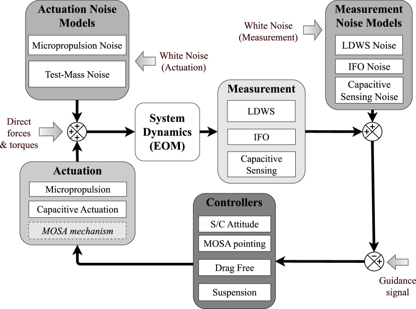
Figure 3: Block diagram of LISA closed-loop dynamics. The system EOM, intrinsically unstable, get stabilized by the application of compensation forces and torques, based on the information from in-loop sensors, and exerted by the actuation system on-board. External disturbances and noise perturb the system, and require the continuous compensation of the control to maintain the DoF at target points. While the current LISANode dynamics simulation includes white noise only, noise models will be inserted, as depicted in this diagram.

Table 2: Table of sensing and actuation noise settings in the simulations. All noises are still assumed to be white in the simulation (apart from test-mass acceleration noise along $\displaystyle x_{1}$ and $\displaystyle x_{2}$), but will account for low-frequency roll-up in upcoming upgrades, as already considered and detailed in [16].

#	Sensing Channel	Noise Floor	Actuation Channel	Noise Floor
1	$\displaystyle x_{1}^{\text{ifo}}\quad/\quad x_{2}^{\text{ifo}}$	$\displaystyle 1.0\times 10^{-12}\,$\displaystyle\mathrm{m}\text{\,}\mathrm{\text{Hz}^{-1/2}}$$	Thrust $\displaystyle X$	$\displaystyle 2.2\times 10^{-7}\,$\displaystyle\mathrm{N}\text{\,}\mathrm{\text{Hz}^{-1/2}}$$
2	$\displaystyle\eta_{1}^{\text{ifo}}\quad/\quad\eta_{2}^{\text{ifo}}$	$\displaystyle 2.0\times 10^{-9}\,$\displaystyle\mathrm{rad}\text{\,}\mathrm{\text{Hz}^{-1/2}}$$	Thrust $\displaystyle Y$	$\displaystyle 1.3\times 10^{-7}\,$\displaystyle\mathrm{N}\text{\,}\mathrm{\text{Hz}^{-1/2}}$$
3	$\displaystyle\phi_{1}^{\text{ifo}}\quad/\quad\phi_{2}^{\text{ifo}}$	$\displaystyle 2.0\times 10^{-9}\,$\displaystyle\mathrm{rad}\text{\,}\mathrm{\text{Hz}^{-1/2}}$$	Thrust $\displaystyle Z$	$\displaystyle 3.6\times 10^{-7}\,$\displaystyle\mathrm{N}\text{\,}\mathrm{\text{Hz}^{-1/2}}$$
4	$\displaystyle x_{1}^{\text{grs}}\quad/\quad x_{2}^{\text{grs}}$	$\displaystyle 1.8\times 10^{-9}\,$\displaystyle\mathrm{m}\text{\,}\mathrm{\text{Hz}^{-1/2}}$$	Thrust $\displaystyle\Theta$	$\displaystyle 7.7\times 10^{-8}\,$\displaystyle\mathrm{N}\text{\,}\mathrm{m}\text{\,}\mathrm{\text{Hz}^{-1/2}}$$
5	$\displaystyle y_{1}^{\text{grs}}\quad/\quad y_{2}^{\text{grs}}$	$\displaystyle 1.8\times 10^{-9}\,$\displaystyle\mathrm{m}\text{\,}\mathrm{\text{Hz}^{-1/2}}$$	Thrust $\displaystyle H$	$\displaystyle 6.9\times 10^{-8}\,$\displaystyle\mathrm{N}\text{\,}\mathrm{m}\text{\,}\mathrm{\text{Hz}^{-1/2}}$$
6	$\displaystyle z_{1}^{\text{grs}}\quad/\quad z_{2}^{\text{grs}}$	$\displaystyle 3.0\times 10^{-9}\,$\displaystyle\mathrm{m}\text{\,}\mathrm{\text{Hz}^{-1/2}}$$	Thrust $\displaystyle\Phi$	$\displaystyle 1.3\times 10^{-7}\,$\displaystyle\mathrm{N}\text{\,}\mathrm{m}\text{\,}\mathrm{\text{Hz}^{-1/2}}$$
7	$\displaystyle\theta_{1}^{\text{grs}}\quad/\quad\theta_{2}^{\text{grs}}$	$\displaystyle 120.0\times 10^{-9}\,$\displaystyle\mathrm{rad}\text{\,}\mathrm{\text{Hz}^{-1/2}}$$	$\displaystyle f_{y}^{\text{grs}}$	$\displaystyle 6.0\times 10^{-15}\,$\displaystyle\mathrm{N}\text{\,}\mathrm{\text{Hz}^{-1/2}}$$
8	$\displaystyle\eta_{1}^{\scriptscriptstyle\text{{ldws}}}\quad/\quad\eta_{2}^{\scriptscriptstyle\text{{ldws}}}$	$\displaystyle 0.2\times 10^{-9}\,$\displaystyle\mathrm{rad}\text{\,}\mathrm{\text{Hz}^{-1/2}}$$	$\displaystyle f_{z}^{\text{grs}}$	$\displaystyle 10.0\times 10^{-15}\,$\displaystyle\mathrm{N}\text{\,}\mathrm{\text{Hz}^{-1/2}}$$
9	$\displaystyle\phi_{1}^{\scriptscriptstyle\text{{ldws}}}\quad/\quad\phi_{2}^{\scriptscriptstyle\text{{ldws}}}$	$\displaystyle 0.2\times 10^{-9}\,$\displaystyle\mathrm{rad}\text{\,}\mathrm{\text{Hz}^{-1/2}}$$	$\displaystyle t_{x}^{\text{grs}}$	$\displaystyle 1.0\times 10^{-15}\,$\displaystyle\mathrm{N}\text{\,}\mathrm{m}\text{\,}\mathrm{\text{Hz}^{-1/2}}$$
10			$\displaystyle t_{y}^{\text{grs}}$	$\displaystyle 1.0\times 10^{-15}\,$\displaystyle\mathrm{N}\text{\,}\mathrm{m}\text{\,}\mathrm{\text{Hz}^{-1/2}}$$
11			$\displaystyle t_{z}^{\text{grs}}$	$\displaystyle 1.0\times 10^{-15}\,$\displaystyle\mathrm{N}\text{\,}\mathrm{m}\text{\,}\mathrm{\text{Hz}^{-1/2}}$$

VI Numerical solving and LISANode simulations

VI.1 LISANode software

LISANode is a graph-based prototype simulator created and used by the LISA collaboration [21, 20]. The graph encoding computations is assembled in Python either from existing graphs or from atomic nodes implemented in C++. The provided Python transcriber is then able to translate the graph into a C++ file encoding the simulation. This ensures the ease-of-use of Python while keeping the performance of C++.

In this work, the library of existing nodes was extended consistently to allow not only scalars to be passed between nodes, but also vectors and $\displaystyle 3\times 3$ matrices. This allows for a much more convenient implementation of the dynamics described here, as well as providing faster execution speeds. Additionally, this enables an easy implementation of differential equation solvers.

VI.2 Linearized Simulation

The linear differential system to be solved can be represented in the continuous state-space formalism, cf. Equation (79). Solving the system in Equation (79) amounts to translating it into a discrete state-space, i.e., the continuous equation of the form

$$\displaystyle\derivative{\overrightarrow{\mathbf{X}}}{t}=A\,\overrightarrow{\mathbf{X}}(t)+B\,\overrightarrow{\mathbf{u}}(t)$$ (82)

with constant $\displaystyle A$ and $\displaystyle B$ into the discrete

$$\displaystyle\overrightarrow{\mathbf{X}}\!\left(t^{(n+1)}\right)=A_{\text{disc.}}\overrightarrow{\mathbf{X}}\!\left(t^{(n)}\right)+B_{\text{disc.}}\overrightarrow{\mathbf{u}}\!\left(t^{(n)}\right)\ .$$ (83)

For completeness, a derivation of the solution can be found in the appendix C. The relevant relations are given by

$$\displaystyle A_{\text{disc.}} \displaystyle=\operatorname{e}^{A\,dt}\ ,$$ (84)

$$\displaystyle B_{\text{disc.}} \displaystyle=A^{-1}\left(\operatorname{e}^{A\,dt}-\mathbb{1}\right)B\ ,$$ (85)

where $\displaystyle dt$ gives the discretization of the time domain, which in this case is given as the inverse of the LISA simulation sampling frequency. With the equations in this form, getting the state vector $\displaystyle\overrightarrow{\mathbf{X}}$ at the next time point amounts to a simple matrix multiplication. As the matrices $\displaystyle A$ and $\displaystyle B$ are known beforehand, the transition to the discrete system can be handled in Python without LISANode. We use an off-the-shelf algorithm for the transformation [24]. In LISANode, the matrix multiplication in each time step is handled within one atomic node to make it more efficient. Finally, discretization of the input vector $\displaystyle\overrightarrow{\mathbf{u}}(t)$ is of importance. The simplest version would be of zero-order hold, i.e., approximating the function with step-functions. A second option would be a first-order hold, i.e., a linear interpolation. We have verified empirically that both methods yield results of equal accuracy, which is likely explained by the high sampling rate used in our simulations ($\displaystyle f_{s}=16\,$\displaystyle\mathrm{Hz}$$) relatively to the typical timescale of our experiments ($\displaystyle<0.1\,$\displaystyle\mathrm{Hz}$$). Hence, we have opted for the simple zero-order interpolation scheme, as given in Equations 84 and 85.

VI.3 Non-linear Simulation

In the non-linear case, the ordinary differential equation system must be solved for each time-step. There are many algorithms available, which usually require the problem to be stated in the form

$$\displaystyle\derivative{\overrightarrow{\mathbf{X}}}{t}=\overrightarrow{\mathbf{f}}(t;\overrightarrow{\mathbf{X}})\ .$$ (86)

The EOM derived here can easily be brought into this form, and the full set can be found in the appendix D. For discretization, we use $\displaystyle dt$ for the step-size again. We chose to implement three algorithms into LISANode, as the graph-based computations made it almost impossible to use an off-the-shelf code. There are different ways to characterize these algorithms, most important is the order of the method in terms of the Local Truncation Error (LTE), i.e., the error done in one time-step, or the Global Truncation Error (GTE), i.e., the error accumulated over multiple time-steps until a final time. Another important aspect is the computational complexity, which here amounts to how many function evaluations of $\displaystyle\overrightarrow{\mathbf{f}}$ are needed to predict the next time-step. We will use the shorthand

$$\displaystyle\overrightarrow{\mathbf{X}}_{n}=\overrightarrow{\mathbf{X}}\!\left(t^{(n)}\right)$$ (87)

for the discretized state vector. The three algorithms considered are:

• Euler Method: The simplest method, which approximates the derivative as a difference quotient

  $$\displaystyle\frac{\overrightarrow{\mathbf{X}}_{n+1}-\overrightarrow{\mathbf{X}}_{n}}{dt} \displaystyle=\overrightarrow{\mathbf{f}}(t;\overrightarrow{\mathbf{X}}_{n})\ ,$$ (88)

  $$\displaystyle\overrightarrow{\mathbf{X}}_{n+1} \displaystyle=dt\cdot\overrightarrow{\mathbf{f}}(t;\overrightarrow{\mathbf{X}}_{n})+\overrightarrow{\mathbf{X}}_{n}\ .$$ (89)

  The method is nevertheless interesting because it is quick (only requires 1 evaluation of $\displaystyle\overrightarrow{\mathbf{f}}$) and gives good results for a small step-size. The LTE is of order $\displaystyle dt^{2}$, the GTE of order $\displaystyle dt$.

• Runge-Kutta 4 (RK4): A commonly used algorithm when it comes to ordinary differential equations. It can be formulated as

  $$\displaystyle\ \ \overrightarrow{\mathbf{X}}_{n+1}=\overrightarrow{\mathbf{X}}_{n}\!+\!\frac{dt}{6}\!\left(\overrightarrow{\mathbf{k}}_{1}+2\overrightarrow{\mathbf{k}}_{2}+2\overrightarrow{\mathbf{k}}_{3}+\overrightarrow{\mathbf{k}}_{4}\right)$$ (90)

  where the $\displaystyle\overrightarrow{\mathbf{k}}_{i}$ depend successively on each other and are given by

  $$\displaystyle\begin{split}\overrightarrow{\mathbf{k}}_{1}&=\overrightarrow{\mathbf{f}}\!\left(t^{(n)};\overrightarrow{\mathbf{X}}_{n}\right)\ ,\\ \overrightarrow{\mathbf{k}}_{2}&=\overrightarrow{\mathbf{f}}\!\left(t^{(n)}+\frac{dt}{2};\overrightarrow{\mathbf{X}}_{n}+\frac{dt}{2}\overrightarrow{\mathbf{k}}_{1}\right)\ ,\\ \overrightarrow{\mathbf{k}}_{3}&=\overrightarrow{\mathbf{f}}\!\left(t^{(n)}+\frac{dt}{2};\overrightarrow{\mathbf{X}}_{n}+\frac{dt}{2}\overrightarrow{\mathbf{k}}_{2}\right)\ ,\\ \overrightarrow{\mathbf{k}}_{4}&=\overrightarrow{\mathbf{f}}\!\left(t^{(n)}+dt;\overrightarrow{\mathbf{X}}_{n}+dt\cdot\overrightarrow{\mathbf{k}}_{3}\right)\ .\end{split}$$ (91)

  It requires 4 function evaluations of $\displaystyle\overrightarrow{\mathbf{f}}$, the LTE is of order $\displaystyle dt^{5}$, and the GTE of order $\displaystyle dt^{4}$.

• Runge-Kutta-Fehlberg 4 (5) (RKF45): This is an interesting extension to RK4. The LTE and GTE are the same for RK4 and RKF45, but by using 6 function evaluations of $\displaystyle\overrightarrow{\mathbf{f}}$ the algorithm can also estimate the local error itself. The estimator is of order $\displaystyle dt^{5}$, hence the name. The constants of the algorithm were chosen in accordance with [25], the scheme is conceptually the same as for RK4, the interdependence of the $\displaystyle\overrightarrow{\mathbf{k}}_{i}$ is more complicated.

Note that due to the LISANode framework, the functions $\displaystyle\overrightarrow{\mathbf{f}}$ are represented by graphs. In the RK4 and RKF45 algorithms, this leads to 4 and 6 copies of this “function graph” due to the interdependence of the $\displaystyle\overrightarrow{\mathbf{k}}_{i}$.

The estimated truncation error of the RKF45 algorithm can be useful to provide an upper bound for the local error, providing an indication of a diverging solution. Its reliability is reduced in the presence of strongly non-linear solutions.

VI.4 Efficiency Analysis

In Table 3 there is a comparison of run times for the linear and non-linear models with different solving algorithms. We chose a simulated time of $\displaystyle 10^{5}$ seconds, but each time-step should take the same amount of time as they each have the same complexity. Thus, the results are presented as speed-ups of simulated time over computation time.

The code has not been fully optimized for run-time yet, and we expect further improvements. Several performance optimizations are possible, e.g. using multiple threads during computation. Thus, the non-linear Euler solver is currently slightly faster than the linear one. We understand this as due to their different implementation: the linear simulation uses a matrix formulation, which requires numerous matrix-vector multiplications. The matrices are quite sparse ($\displaystyle\sim\!5\%$ non-zero elements), which results in some overhead compared to the non-linear Euler implementation.

Table 3: Table comparing computation time of the linear and non-linear implementations with different solving algorithms. The results are given as dimensionless ratios of simulated time and computation time, i.e., how much speed-up is gained in the simulation. For a factor $\displaystyle 100$ this means that it takes $\displaystyle 0.01$ seconds on a computer to simulate $\displaystyle 1$ second in the model. All numbers are generated using an Apple M1 Pro processor (single-thread execution) with the native clang compiler with optimization level 1.

Simulation	Linear	NL (Euler)	NL (RK4)	NL (RKF45)
Single S/C	513	635	373	296
Full LISA	65.6	84.4	64.8	52.3

VII Simulation experiments

Solving the 17-dimensional differential systems, the simulation yields the time evolution of all the system dynamical DoFs, as well as the in-loop sensor outputs, the commanded and applied forces on each dynamical body. In addition, the possibility of injecting (sinusoidal) excitation signals is implemented, such as disturbance signals $\displaystyle\overrightarrow{\mathbf{d}}$ (“direct forces & torques” in Figure 3) or guidance signals $\displaystyle\overrightarrow{\mathbf{g}}$ (biasing the in-loop sensors, see Figure 3). These input ports are useful to probe the closed-loop transfer functions of the system and perform experiments to check the dynamical model. This is the purpose of this section.

We present a series of $\displaystyle 8$ simulated experiments realized on-board a single spacecraft, where excitation signals are injected in the closed-loop to stimulate the dynamics and probe its response to disturbances. We inject $\displaystyle 3$ guidance signal injections simultaneously at $\displaystyle 3$ distinct frequencies, and for $\displaystyle 8$ different injection amplitudes:

• On spacecraft control angle $\displaystyle H$:
  at $\displaystyle f_{g_{H}}=1\,$\displaystyle\mathrm{mHz}$$, amplitude:
  $\displaystyle A_{g_{H}}=\big{[}10^{5},10^{4},10^{3},100,10,1,0.1,10^{-2}\big{]}\,$\displaystyle\mathrm{\SIUnitSymbolMicro rad}$$

• On test-mass longitudinal $\displaystyle x$-displacement $\displaystyle x_{1}$:
  at $\displaystyle f_{g_{x_{1}}}=5\,$\displaystyle\mathrm{mHz}$$, amplitude:
  $\displaystyle A_{g_{x_{1}}}=\big{[}10^{5},10^{4},10^{3},100,10,1,0.1,10^{-2}\big{]}\,$\displaystyle\mathrm{\SIUnitSymbolMicro m}$$

• On test-mass longitudinal $\displaystyle x$-displacement $\displaystyle x_{2}$:
  at $\displaystyle f_{g_{x_{2}}}=10\,$\displaystyle\mathrm{mHz}$$, amplitude:
  $\displaystyle A_{g_{x_{2}}}=\big{[}10^{5},10^{4},10^{3},100,10,1,0.1,10^{-2}\big{]}\,$\displaystyle\mathrm{\SIUnitSymbolMicro m}$$

We refer the reader to the Figure 2 helping the visualization of the DoFs and of the geometry of these experiments. These five injection experiments are realized with both linear and non-linear models for comparison. The simulations have a duration of $\displaystyle 3\times 10^{4}\,$\displaystyle\mathrm{s}$$ and are sampled to $\displaystyle 4\,$\displaystyle\mathrm{Hz}$$ each, from which the first $\displaystyle 1\times 10^{4}\,$\displaystyle\mathrm{s}$$ have been truncated, ensuring the slow MOSA control has stabilized fully and the steady-state regime has been reached. The residual time-series (between linear and non-linear simulations) are computed for each experiment. Figures 4 and 5 show the simulation results for the largest amplitude experiments ($\displaystyle A_{g_{H}}=10.0\,$\displaystyle\mathrm{\SIUnitSymbolMicro rad}$$, $\displaystyle A_{g_{x_{1}}}=A_{g_{x_{2}}}=10.0\,$\displaystyle\mathrm{\SIUnitSymbolMicro m}$$).

VII.1 Testing spacecraft dynamics

Figure 4 shows the spacecraft angular DoFs time series $\displaystyle\left[\Theta(t),H(t),\Phi(t)\right]$ for the linear (blue) and the non-linear (orange) simulations. The green traces give the residuals. We observe the $\displaystyle 10.0\,$\displaystyle\mathrm{\SIUnitSymbolMicro rad}$$ $\displaystyle H$ injections around the $\displaystyle Y$-axis as expected. $\displaystyle\Theta$ and $\displaystyle\Phi$ are compatible with simulated noise (sensing and actuation noise). The linear and non-linear simulations use different realizations of the noise, explaining the shape of the observed residual, which yields the sum of the uncorrelated noise. The $\displaystyle H$ time series at the center shows an excellent agreement between linear and non-linear simulations. This will be investigated more quantitatively with the test-mass longitudinal motion.

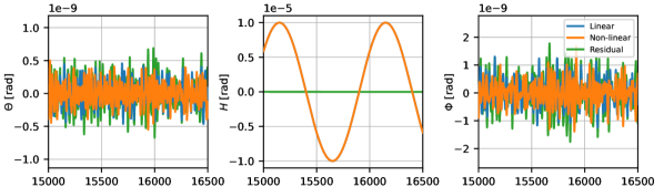
Figure 4: Time evolution of the spacecraft $\displaystyle 3$ DoFs (angular $\displaystyle[\Theta,H,\Phi]$) during the largest amplitude injection experiment. Guidance signals are injected on the spacecraft angle $\displaystyle H$, and test-masses $\displaystyle x_{1}$ and $\displaystyle x_{2}$ controlled DoFs, respectively of amplitude $\displaystyle 10\,$\displaystyle\mathrm{\SIUnitSymbolMicro rad}$$, $\displaystyle 10\,$\displaystyle\mathrm{\SIUnitSymbolMicro m}$$ and $\displaystyle 10\,$\displaystyle\mathrm{\SIUnitSymbolMicro m}$$ at $\displaystyle f=1\,$\displaystyle\mathrm{mHz}$$, $\displaystyle 5\,$\displaystyle\mathrm{mHz}$$, and $\displaystyle 10\,$\displaystyle\mathrm{mHz}$$. Simulations using the linear (in blue) and non-linear (orange) closed-loop system model are shown, together with the modeling residual (in green).

VII.2 Testing test-mass dynamics

Test-mass motion has more complex dynamics properties to probe since it is impacted by both spacecraft (lever arms, inertial forces, rotations in housing) and test-mass disturbances. Hence, in the Figure 5 one sees the imprint of the three injections altogether. While drag-free control suppresses (lever-arm) spacecraft-rotation-driven longitudinal motion of the test-masses, the stimulated rotation of spacecraft is observable on both $\displaystyle\theta$ and $\displaystyle\phi$ rotational DoFs of the test-masses, since the $\displaystyle Y$-axis of the spacecraft $\displaystyle\mathcal{B}$-frame, around which the spacecraft rotation is performed, has non-zero components along the $\displaystyle x$ and $\displaystyle y$ axes of the housing frames $\displaystyle\mathcal{H}_{1}$ and $\displaystyle\mathcal{H}_{2}$. The excitation signal is amplified compared to the stimulation signal, exceeding $\displaystyle 10\,$\displaystyle\mathrm{\SIUnitSymbolMicro rad}$$ for $\displaystyle\eta_{1}$. This is coincidentally due to the injection frequency $\displaystyle f_{g_{H}}=1\,$\displaystyle\mathrm{mHz}$$ sitting at the end of the suspension control bandwidth (see Table III. of [16] for more details), where the suspension struggles to compensate for external disturbances, amplifying them in a narrow bandwidth around the millihertz. We have verified that, when injecting at the lower frequency of $\displaystyle f_{g_{H}}=0.1\,$\displaystyle\mathrm{mHz}$$, where suspension control is still efficient, the imprint of the injection on $\displaystyle\theta_{1}$ and $\displaystyle\eta_{1}$ is mitigated down to below $\displaystyle 0.1\,$\displaystyle\mathrm{\SIUnitSymbolMicro rad}$$, and the test-masses are well forced to rotate together with the spacecraft guidance at low frequency [16].

The top subplots of Figure 5 show the longitudinal motion time series, where the $\displaystyle x_{1}$ and $\displaystyle x_{2}$ guidance injections are visible. The left-hand plot shows the $\displaystyle x_{1}$ DoF time series, which indicates that the drag-free control is doing well to force this dynamical DoF to track the guidance sinusoidal injection. The middle plot shows the $\displaystyle y_{1}$ DoF which exhibits a composition of the two injection frequencies, as an imprint of both $\displaystyle x_{1}$ and $\displaystyle x_{2}$ time-evolution. Indeed, drag-free control here has the task to force $\displaystyle x_{1}$ and $\displaystyle x_{2}$ variables to track down two different frequencies, despite $\displaystyle\hat{\mathbf{e}}_{x_{\scriptscriptstyle 1}}$ and $\displaystyle\hat{\mathbf{e}}_{x_{\scriptscriptstyle 2}}$ being not perpendicular. In practice, the command will then have to request compensation of spacecraft motion along $\displaystyle x_{2}$ in order to correct $\displaystyle f_{x_{1}}$ injected motion along $\displaystyle x_{2}$ originating from the $\displaystyle x_{1}$ control, which has necessarily leaked to the $\displaystyle x_{2}$ direction due to the non-orthogonality between $\displaystyle\hat{\mathbf{e}}_{x_{\scriptscriptstyle 1}}$ and $\displaystyle\hat{\mathbf{e}}_{x_{\scriptscriptstyle 2}}$. This explains why one sees traces of both frequencies in the $\displaystyle y_{1}$ plot of Figure 5. All the dynamics take place in the $\displaystyle XOY$ plane here; the $\displaystyle z_{1}$ dynamical DoF time-series are compatible with noise in this case. Again, Figure 5 is presenting the largest amplitude injection experiment, showing excellent agreement between the linear and non-linear simulation. There are, however, observable discrepancies when the quantities—and in particular the residuals—are represented in the frequency domain. In the next section, we show that the observed discrepancies indicate the presence of dynamical time-varying and non-linear features the Linear Time-Invariant (LTI) model is failing to capture by construction.

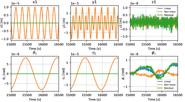
Figure 5: Time evolution of the test-mass $\displaystyle 6$ DoFs (longitudinal $\displaystyle[x_{1},y_{1},z_{1}]$ on the top subplots, angular $\displaystyle[\theta_{1},\eta_{1},\phi_{1}]$ on the bottom subplots) during the largest amplitude injection experiment. Guidance signals are injected on spacecraft angle $\displaystyle H$, and test-masses $\displaystyle x_{1}$ and $\displaystyle x_{2}$ controlled DoFs, respectively of amplitude $\displaystyle 10\,$\displaystyle\mathrm{\SIUnitSymbolMicro rad}$$, $\displaystyle 10\,$\displaystyle\mathrm{\SIUnitSymbolMicro m}$$ and $\displaystyle 10\,$\displaystyle\mathrm{\SIUnitSymbolMicro m}$$ at $\displaystyle f=1\,$\displaystyle\mathrm{mHz}$$, $\displaystyle 5\,$\displaystyle\mathrm{mHz}$$, and $\displaystyle 10\,$\displaystyle\mathrm{mHz}$$. Simulations using the linear (in blue) and non-linear (orange) closed-loop system model are shown, together with the modeling residual (in green).

VII.3 Resolution of non-linearities

Computing the frequency spectra of the time series in Figure 5, discrepancies between linear and non-linear simulations become visible. This is quantified using the relative error of spectrum amplitudes at injection frequencies

$$\delta_{\text{res}}=\absolutevalue{\frac{\absolutevalue{\tilde{X}^{\text{nl}}(f_{\text{inj}})}-\absolutevalue{\tilde{X}^{\text{l}}(f_{\text{inj}})}}{\absolutevalue{\tilde{X}^{\text{l}}(f_{\text{inj}})}}}\ .$$ (92)

Figure 6 shows the behavior of the relative error $\displaystyle\delta_{\text{res}}$ as a function of the injection amplitudes. Specific simulations with sensing and actuation noise turned off have been realized for this analysis, to better resolve small discrepancies between the linear and non-linear models. Figure 6 focuses on the dynamical behavior of the DoF $\displaystyle x_{1}$, inspected at two different injection frequencies: $\displaystyle f_{g_{x_{1}}}$ and $\displaystyle 2\ f_{g_{H}}$. The top subplot shows agreement between the linear and non-linear model of the response to the $\displaystyle x_{1}$ guidance signals at $\displaystyle f_{g_{x_{1}}}=5\,$\displaystyle\mathrm{mHz}$$. The residual scales linearly w.r.t. the injection amplitude: it is the signature of the contribution of an extra linear component the linear model is missing. Indeed, the linear model discussed is also time-invariant (see Section IV.3). Hence, it cannot account for time-variability of the dynamical system such as the MOSA rotation, which can have an important impact on geometrical projections and inertial response to external input forces and torques. In the particular case of Figure 6, the discrepancy comes from the MOSA opening angle departing from $\displaystyle 60$\displaystyle\mathrm{\SIUnitSymbolDegree}$$ in the non-linear model, since only the latter accounts for telescope pointing constrained by the satellite’s orbital motion. The linear simulation stays ignorant of such feature, hence inducing a small projection error.

On the other hand, the bottom subplot of Figure 6 presents the non-linear behavior of the $\displaystyle x_{1}$ DoF dynamics, in particular its response to spacecraft rotational excitation. It shows that when the spacecraft is forced to rotate around its $\displaystyle Y$-axis above an amplitude of $\displaystyle A_{g_{H}}=0.1\,$\displaystyle\mathrm{mrad}$$, a quadratic component dominates the response to the rotational excitation, as we observe a trend in the $\displaystyle\delta x_{1}$ residual proportional to $\displaystyle A_{g_{H}}^{2}$. Note that, here, the frequency inspected is twice of the angular injection frequency, since the non-linear response manifests as additional signal harmonics. Since the linear response cannot create a $\displaystyle 2f_{g_{H}}$ signal, the relative error at $\displaystyle 2f_{g_{H}}$ is $\displaystyle\delta x_{1}\approx 1.0$ for $\displaystyle A_{g_{H}}\leq 10\,$\displaystyle\mathrm{\SIUnitSymbolMicro rad}$$.

Figure 6 hence verifies that the LTI modeling is indeed not, by construction, capable of capturing non-linear or time-varying dynamical terms, since all quadratic terms have been truncated when the state-space matrices have been evaluated at working points (cf. section IV.3), and the time-varying components averaged out over the simulation duration. The residuals observed in Figure 6 are the residuals of this truncation, and this motivates the introduction of the non-linear modeling, for instance, in the context of system identification experiments involving large probing signals.

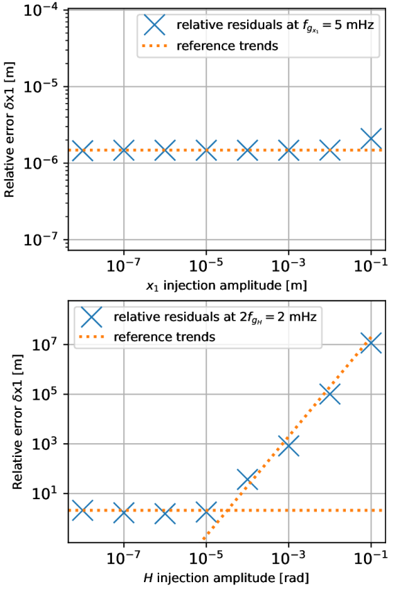
Figure 6: Measured relative errors of the $\displaystyle\delta x_{1}$ DoF between linear and non-linear simulations, for the range of eight excitation amplitudes covered. The blue crosses $\displaystyle\times$ show the measurements of the error at $\displaystyle f=10\,$\displaystyle\mathrm{mHz}$$ corresponding to the $\displaystyle g_{x_{1}}$ longitudinal injection frequency (top subplot), and $\displaystyle f=2\,$\displaystyle\mathrm{mHz}$$ corresponding to twice the $\displaystyle g_{H}$ angular injection frequency (bottom subplot). The orange curves represent linear reference trends in log-log scale, facilitating the reading of the order of dependence of the dynamical response to the injection amplitude scale. On the top subplot, the relative error $\displaystyle\delta x_{1}$ stays constant w.r.t. the scale of the excitation, and is the consequence of a time-varying component the LTI model cannot capture, such as the time-varying opening angle between MOSAs. On the bottom plot, we observe a relative error that scales quadratically with the excitation signal $\displaystyle g_{H}$ after $\displaystyle A_{g_{H}}=0.1\,$\displaystyle\mathrm{mrad}$$. It reflects the linear nature of the LTI model, unable to capture non-linear dynamical contributions such as the inertial forces exerting on test mass along $\displaystyle x_{1}$ and induced by the spacecraft angular jitter.

VIII TDI and S/C jitter suppression: a numerical demonstration

VIII.1 Time-Delay Interferometry and Dynamics

A variety of noise sources, in particular the spacecraft thrusters, are expected to create random motion, or “jitter”, between the test-masses and spacecraft. In addition to suppressing the laser frequency noise, one of the goals of TDI is to suppress the influence of the spacecraft jitter, by cancelling equal and opposite effects in the long and short-arm IFOs. With an ideal instrument, e.g., in the absence of tilt-to-length couplings, the test-mass interferometer will capture all the spacecraft noisy accelerations along the long-range interferometer. Hence, combining the signals within the TDI scheme will result in the cancellation of this contribution. Again, the situation just described is idealized, and misalignment between test-mass and long-range interferometer axes, as well as reference points mismatch (see section VIII.3), will let jitter residuals through that one can interpret as geometrical tilt-to-length effects. In this subsection, however, we will restrict our analysis to the ideal, no-TTL case, and utilize the jitter suppression expectation as a figure-of-merit for demonstrating the correct interfacing between the dynamical model and optical interferences on-board and across the constellation.

VIII.2 Interferometer observables

The simulator delivers time-series of the metrology sensors on-board each spacecraft. It also yields Mother-Nature quantities such as the actual velocity $\displaystyle v_{\scriptscriptstyle T_{\scriptscriptstyle 1}/H_{\scriptscriptstyle 1}}^{\scriptscriptstyle\mathcal{H}_{\scriptscriptstyle 1}}$ and $\displaystyle v_{\scriptscriptstyle T_{\scriptscriptstyle 2}/H_{\scriptscriptstyle 2}}^{\scriptscriptstyle\mathcal{H}_{\scriptscriptstyle 2}}$ of the test-masses w.r.t. the housing frames $\displaystyle\mathcal{H}_{\scriptscriptstyle 1}$ and $\displaystyle\mathcal{H}_{\scriptscriptstyle 2}$, or the true acceleration $\displaystyle\overrightarrow{{\bf\it a}}_{\scriptscriptstyle B}=\tfrac{\overrightarrow{{\bf\it f}}_{\scriptscriptstyle B}}{m_{B}}$ of the spacecraft CoM w.r.t. its local inertial frame, which can be projected along the interferometer long-arm axes

$$\displaystyle a_{1}=\frac{\overrightarrow{{\bf\it f}}_{\scriptscriptstyle B}}{m_{B}}\cdot\overrightarrow{{\bf\it e}}_{\scriptscriptstyle\mathcal{H}_{\scriptscriptstyle 1}^{*},x}\ , \displaystyle a_{2}=\frac{\overrightarrow{{\bf\it f}}_{\scriptscriptstyle B}}{m_{B}}\cdot\overrightarrow{{\bf\it e}}_{\scriptscriptstyle\mathcal{H}_{\scriptscriptstyle 2}^{*},x}\ .$$ (93)

These physical quantities are measured by the local interferometers (TMI) and the inter-spacecraft, long-arm interferometers (ISI) respectively. They provide the dynamics contributions to the phase modulation of the heterodyne interferometers beat notes, once post-processed and rescaled into equivalent frequency fluctuation units w.r.t to the laser carrier frequency as

$$\displaystyle\nu_{\scriptscriptstyle 12}^{\text{tmi}}\approx\frac{v_{\scriptscriptstyle T_{\scriptscriptstyle 1}/H_{\scriptscriptstyle 1}}^{\scriptscriptstyle\mathcal{H}_{\scriptscriptstyle 1}}}{c}\ , \displaystyle\nu_{\scriptscriptstyle 13}^{\text{tmi}}\approx\frac{v_{\scriptscriptstyle T_{\scriptscriptstyle 2}/H_{\scriptscriptstyle 2}}^{\scriptscriptstyle\mathcal{H}_{\scriptscriptstyle 2}}}{c}\ ,$$ (94)

$$\displaystyle\nu_{\scriptscriptstyle 12}^{\text{isi}}\approx\frac{1}{c}\int_{t_{0}}^{t}{a_{1}dt^{\prime}}\ , \displaystyle\nu_{\scriptscriptstyle 13}^{\text{isi}}\approx\frac{1}{c}\int_{t_{0}}^{t}{a_{2}dt^{\prime}}\ .$$ (95)

Figure 7: The overall test-mass-to-test-mass optical measurement is split into three pieces: one ISI and two TMI s per arm. Nominally, local spacecraft (1) accelerations towards the distant spacecraft (2) shorten the ISI optical path, but increase the local TMI optical path length by the same amount, thus TDI outputs remain unaffected. In this nominal case, the geometrical point of the spacecraft probed by the ISI is matching the one probed by the TMI. We denoted such a geometrical point by the letter $\displaystyle C$. Illustration from [16].

VIII.3 What does spacecraft jitter mean?

Particular attention must be set on the definition of the spacecraft acceleration used in Equation (93). Indeed, one still needs to identify the geometrical point of the spacecraft whose noisy dynamical motion contributes to the ISI beat note in Equation (95)—a geometrical point that we will denote with the letter $\displaystyle C$ from now on. That is, not only does the CoM longitudinal noisy motion contribute to $\displaystyle\nu_{\text{isi}}$, but so does the spacecraft rotational motion around its CoM which translates into a translational acceleration of the point $\displaystyle C$ relative to its local inertial frame. Accounting for such a lever-arm effect, Equation (95) now becomes

$$\displaystyle\nu_{\scriptscriptstyle 12}^{\text{isi}}\approx\frac{1}{c}\left[\int_{t_{0}}^{t}{a_{1}dt^{\prime}}\ -\ \left(\overrightarrow{{\bf\it\omega}}_{\scriptscriptstyle\mathcal{B}/\mathcal{O}}\times\overrightarrow{{\bf\it r}}_{\scriptscriptstyle C_{\scriptscriptstyle{\scriptscriptstyle 1}}/B}\right)\cdot\overrightarrow{{\bf\it e}}_{\scriptscriptstyle\mathcal{H}_{1}^{*},x}\right]\,,$$ (96)

$$\displaystyle\nu_{\scriptscriptstyle 13}^{\text{isi}}\approx\frac{1}{c}\left[\int_{t_{0}}^{t}{a_{2}dt^{\prime}}\ -\ \left(\overrightarrow{{\bf\it\omega}}_{\scriptscriptstyle\mathcal{B}/\mathcal{O}}\times\overrightarrow{{\bf\it r}}_{\scriptscriptstyle C_{\scriptscriptstyle{\scriptscriptstyle 2}}/B}\right)\cdot\overrightarrow{{\bf\it e}}_{\scriptscriptstyle\mathcal{H}_{2}^{*},x}\right]\,.$$ (97)

As confirmed by simulations, the nominal location for $\displaystyle C_{\scriptscriptstyle 1}$ and $\displaystyle C_{\scriptscriptstyle 2}$ are actually the housing centers $\displaystyle H_{\scriptscriptstyle 1}$ and $\displaystyle H_{\scriptscriptstyle 2}$, in order to suppress large geometrical tilt-to-length, deteriorating detector sensitivity significantly beyond requirements. In such a nominal case, the geometrical point of any local spacecraft imaged to the distant spacecraft corresponds to the nominal position of the test-masses, and the test-mass to test-mass optical measurement can be reconstituted independently of the spacecraft dynamics.

VIII.4 Simulating spacecraft jitter suppression

We performed a series of simulation runs using LISANode to demonstrate this suppression. We use the PyTDI software [26] to build the TDI data streams out of the interferometer beat notes generated by LISANode, while LISAOrbits Python software [27] is utilized to compute the light travel times between spacecraft required for PyTDI computations. Figure 8 shows the TDI-X spectrum for 4 simulations: A run using default, expected values for all noise (orange), disabling noise on the Micro-Propulsion System (green), disabling dynamics entirely (red), and finally default noise with disabled TMI channel (filled zith $\displaystyle 0$’s) to emulate a failure of spacecraft and MOSA jitters correction by TDI (blue). In all but the latter case, the summing method used by TDI reduces the error to a comparable level. In the final case, as expected, the post-processing combination of TMI and ISI cannot isolate the long-range measurement from spacecraft jitter, which starts to impact significantly the sensitivity around $\displaystyle 4\,$\displaystyle\mathrm{mHz}$$—above the drag-free frequency bandwidth. It results in greater noise leaking into the TDI channels in this case.

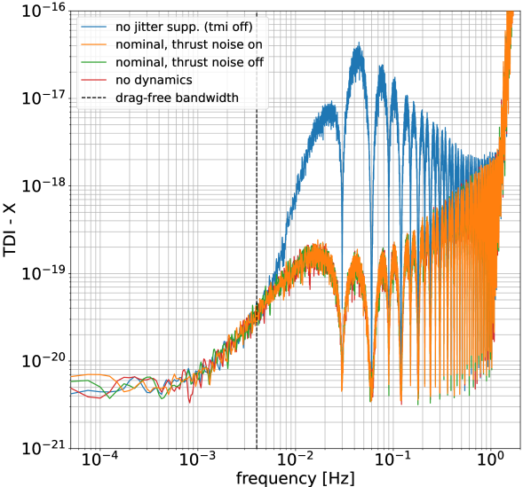
Figure 8: Spectrum of TDI-X channel in four different analysis cases: no dynamics data (red), thrust noise on (orange) and off (green), no jitter information from local test-mass IFO (blue). This plot demonstrates TDI efficiency of suppressing realistic spacecraft longitudinal and angular jitters.

Hence, the blue curve provides an estimate of how the spacecraft jitter would impact LISA sensitivity in the case where TDI would not be efficient at isolating the detector performance from spacecraft dynamics noise or in the case of a failure in the TMI. The green and red traces are both giving the no spacecraft jitter reference curve: in the first case, force noise on spacecraft is essentially turned off, while in the second case, there are no spacecraft dynamics modelled in the first place, so no jitter exists by construction. Figure 8 then shows that the orange curve, including both force noise on spacecraft and a correct set-up for TDI, lines up well with the no jitter reference spectra, demonstrating that TDI is mitigating efficiently the spacecraft jitter, and bringing it down to subdominant contributions. It is the first numerical demonstration of TDI jitter suppression within a full, time-domain LISA simulation.

IX Conclusion

With this work, we provide a comprehensive framework for describing mathematically the closed-loop dynamics of the $\displaystyle 3\times 17$ DoFs at play in the LISA constellation system. We have derived the differential EOM s for the longitudinal and rotational DoFs of the moving bodies, both in a vectorial form (Equation (51), (48), (53), (58)) and expressed in coordinate systems of interest specified in section II.1 (Equation (70), (69), (71), (72)). These EOM were inserted in a Multiple-Input Multiple-Output (MIMO) feedback system, interfaced with sensors, actuators, controllers, and noise sources within a control loop, the so-called DFACS loop (cf. section V). The resulting MIMO differential system has been solved using several numerical schemes, depending on whether the system dynamics was linearized or not. For linear systems, semi-analytical solutions are available, while for the full non-linear simulations, we have preferred Runge-Kutta 4 numerical solving scheme (cf. section VI). In section VII, the simulation physics has been probed and interpreted with a selection of injection experiments, and we have illustrated the excellent agreement between the linear and the non-linear simulations, the existing residual being consistent with time-varying and non-linear dynamical contributions the LTI model cannot capture (see Figure 6). Finally, in section VIII, we have discussed the non-trivial interface between the simulated physical quantities (spacecraft and test-mass accelerations) with the interferometers’ beat notes, and concluded with the numerical demonstration that the TDI algorithm can suppress spacecraft and MOSA noisy motion from the final interferometer data streams, in the idealized case where no dynamical couplings (TTL, actuation cross-talks, stiffnesses) are turned on.

This first End-To-End simulation offers the opportunity to start quantitatively evaluating and optimizing post-processing techniques aimed at suppressing dynamical jitters’ imprints on TDI data streams (TTL mitigation, glitch detection and suppression). More generally, it enables the study of the impact of artifacts of dynamical origin (jitter noise, micrometeoroids hitting the spacecraft [28]) and propagating due to physical couplings such as TTL or stiffness forces [29, 18], through the instrument response and all the way down to the TDI time series. It breaks down and reproduces the complex interplay between the DFACS response, the propagation time-delays and various echo phenomena due to post-processing which transforms an impulse excitation signal into a much richer signature. Because LISA will open a novel window on the Universe, potentially capturing unexpected, transient signals, it is crucial to characterize instrumental artifacts with the best accuracy to discriminate instrumental from astrophysical events. This E2E simulation will provide key information to that end. We finally note that all the codes and the software dependencies (LISAOrbits, PyTDI, …) are available (on-demand) to the consortium in the my-lisanode-sim Gitlab repository, from which one can download the full environment encapsulated in a docker or a singularity container and from which one can run the E2E and reproduce the results hereby presented (dedicated experiment scripts are also provided).

X Acknowledgement

Lavinia Heisenberg would like to acknowledge financial support from the European Research Council (ERC) under the European Unions Horizon 2020 research and innovation programme grant agreement No 801781 and by the Swiss National Science Foundation grant 179740. LH further acknowledges support from the Deutsche Forschungsgemeinschaft (DFG, German Research Foundation) under Germany’s Excellence Strategy EXC 2181/1 - 390900948 (the Heidelberg STRUCTURES Excellence Cluster). Henri Inchauspé would like to acknowledge the Centre Nationale d’Études Spatiales (CNES) for its financial support. Peter Wass, Orion Sauter and Henri Inchauspé were supported by NASA LISA Preparatory Science program, grant number 80NSSC19K0324. Numerical computations were performed on the DANTE platform, APC, France.

Appendix A Angular velocity and acceleration from basis vectors

In this appendix, we derive an analytical expression of the angular velocity of the body as a function of the unit vectors basis of a reference frame attached rigidly to the body.

Using the transport theorem at Equation 1 as well as cross-product properties, it can be found that

$$\displaystyle\begin{split}\derivative{t}\Bigg{|}_{\scriptscriptstyle\mathcal{J}}\mspace{-10.0mu}\left[\hat{\mathbf{e}}_{x,\mathcal{B}}\right]&=\derivative{t}\Bigg{|}_{\scriptscriptstyle\mathcal{B}}\mspace{-10.0mu}\left[\hat{\mathbf{e}}_{x,\mathcal{B}}\right]+\overrightarrow{{\bf\it\omega}}_{\scriptscriptstyle B/J}\times\hat{\mathbf{e}}_{x,\mathcal{B}}\\ &=\overrightarrow{{\bf\it\omega}}_{\scriptscriptstyle B/J}\times\hat{\mathbf{e}}_{x,\mathcal{B}}\,,\end{split}$$ (98)

$$\displaystyle\begin{split}\derivative{t}\Bigg{|}_{\scriptscriptstyle\mathcal{J}}\mspace{-10.0mu}\left[\hat{\mathbf{e}}_{y,\mathcal{B}}\right]&=\derivative{t}\Bigg{|}_{\scriptscriptstyle\mathcal{B}}\mspace{-10.0mu}\left[\hat{\mathbf{e}}_{y,\mathcal{B}}\right]+\overrightarrow{{\bf\it\omega}}_{\scriptscriptstyle B/J}\times\hat{\mathbf{e}}_{y,\mathcal{B}}\\ &=\overrightarrow{{\bf\it\omega}}_{\scriptscriptstyle B/J}\times\hat{\mathbf{e}}_{y,\mathcal{B}}\,,\end{split}$$ (99)

$$\displaystyle\begin{split}\derivative{t}\Bigg{|}_{\scriptscriptstyle\mathcal{J}}\mspace{-10.0mu}\left[\hat{\mathbf{e}}_{z,\mathcal{B}}\right]&=\derivative{t}\Bigg{|}_{\scriptscriptstyle\mathcal{B}}\mspace{-10.0mu}\left[\hat{\mathbf{e}}_{z,\mathcal{B}}\right]+\overrightarrow{{\bf\it\omega}}_{\scriptscriptstyle B/J}\times\hat{\mathbf{e}}_{z,\mathcal{B}}\\ &=\overrightarrow{{\bf\it\omega}}_{\scriptscriptstyle B/J}\times\hat{\mathbf{e}}_{z,\mathcal{B}}\,,\end{split}$$ (100)

which simplify since the basis vectors appear static in the body frame $\displaystyle\mathcal{B}$ by definition. We now cross-multiply both sides by its respective basis

$$\displaystyle\hat{\mathbf{e}}_{x,\mathcal{B}}\times\derivative{t}\Bigg{|}_{\scriptscriptstyle\mathcal{J}}\mspace{-10.0mu}\left[\hat{\mathbf{e}}_{x,\mathcal{B}}\right]=\hat{\mathbf{e}}_{x,\mathcal{B}}\times\overrightarrow{{\bf\it\omega}}_{\scriptscriptstyle B/J}\times\hat{\mathbf{e}}_{x,\mathcal{B}}\,,$$ (101)

$$\displaystyle\hat{\mathbf{e}}_{y,\mathcal{B}}\times\derivative{t}\Bigg{|}_{\scriptscriptstyle\mathcal{J}}\mspace{-10.0mu}\left[\hat{\mathbf{e}}_{y,\mathcal{B}}\right]=\hat{\mathbf{e}}_{y,\mathcal{B}}\times\overrightarrow{{\bf\it\omega}}_{\scriptscriptstyle B/J}\times\hat{\mathbf{e}}_{y,\mathcal{B}}\,,$$ (102)

$$\displaystyle\hat{\mathbf{e}}_{z,\mathcal{B}}\times\derivative{t}\Bigg{|}_{\scriptscriptstyle\mathcal{J}}\mspace{-10.0mu}\left[\hat{\mathbf{e}}_{z,\mathcal{B}}\right]=\hat{\mathbf{e}}_{z,\mathcal{B}}\times\overrightarrow{{\bf\it\omega}}_{\scriptscriptstyle B/J}\times\hat{\mathbf{e}}_{z,\mathcal{B}}\,.$$ (103)

From Lagrange’s vector triple product formula: $\displaystyle\mathbf{a}\times(\mathbf{b}\times\mathbf{c})=(\mathbf{a}\cdot\mathbf{c})\mathbf{b}-(\mathbf{a}\cdot\mathbf{b})\mathbf{c}$, and adding up Equations 101 - 103, we find

$$\displaystyle\begin{split}&\hat{\mathbf{e}}_{x,\mathcal{B}}\times\derivative{t}\Bigg{|}_{\scriptscriptstyle\mathcal{J}}\mspace{-10.0mu}\left[\hat{\mathbf{e}}_{x,\mathcal{B}}\right]+\hat{\mathbf{e}}_{y,\mathcal{B}}\times\derivative{t}\Bigg{|}_{\scriptscriptstyle\mathcal{J}}\mspace{-10.0mu}\left[\hat{\mathbf{e}}_{y,\mathcal{B}}\right]\\ &+\hat{\mathbf{e}}_{z,\mathcal{B}}\times\derivative{t}\Bigg{|}_{\scriptscriptstyle\mathcal{J}}\mspace{-10.0mu}\left[\hat{\mathbf{e}}_{z,\mathcal{B}}\right]\\ &=3\,\overrightarrow{{\bf\it\omega}}_{\scriptscriptstyle\mathcal{B}/\mathcal{J}}-\omega_{\scriptscriptstyle x,\mathcal{B}/\mathcal{J}}^{\scriptscriptstyle\mathcal{B}}\ \hat{\mathbf{e}}_{x,\mathcal{B}}-\omega_{\scriptscriptstyle y,\mathcal{B}/\mathcal{J}}^{\scriptscriptstyle\mathcal{B}}\ \hat{\mathbf{e}}_{y,\mathcal{B}}\\ &\ \ \ -\omega_{\scriptscriptstyle z,\mathcal{B}/\mathcal{J}}^{\scriptscriptstyle\mathcal{B}}\ \hat{\mathbf{e}}_{z,\mathcal{B}}\\ &=2\,\overrightarrow{{\bf\it\omega}}_{\scriptscriptstyle\mathcal{B}/\mathcal{J}}\ .\end{split}$$ (104)

This leads to the final equation for angular velocity

$$\displaystyle\begin{split}\overrightarrow{{\bf\it\omega}}_{\scriptscriptstyle\mathcal{B}/\mathcal{J}}=&\frac{1}{2}\ \hat{\mathbf{e}}_{x,\mathcal{B}}\times\derivative{t}\Bigg{|}_{\scriptscriptstyle\mathcal{J}}\mspace{-10.0mu}\left[\hat{\mathbf{e}}_{x,\mathcal{B}}\right]\\ &+\frac{1}{2}\ \hat{\mathbf{e}}_{y,\mathcal{B}}\times\derivative{t}\Bigg{|}_{\scriptscriptstyle\mathcal{J}}\mspace{-10.0mu}\left[\hat{\mathbf{e}}_{y,\mathcal{B}}\right]\\ &+\frac{1}{2}\ \hat{\mathbf{e}}_{z,\mathcal{B}}\times\derivative{t}\Bigg{|}_{\scriptscriptstyle\mathcal{J}}\mspace{-10.0mu}\left[\hat{\mathbf{e}}_{z,\mathcal{B}}\right]\ .\end{split}$$ (105)

Appendix B Full derivation of equations of motion for non-static mass distribution

In the main part of this document, we have considered a fully static mass distribution of the satellite system in its body frame. However, since the two MOSA on-board will rotate accounting for yearly breathing of the constellation, all masses within the spacecraft are not strictly static w.r.t. the $\displaystyle\mathcal{B}$-frame. As a result, the CoM will be non-stationnary in the body frame $\displaystyle\mathcal{B}$. To model this extra physical feature, it is convenient to define a new geometrical point, denoted $\displaystyle S$, which corresponds to the CoM of the spacecraft platform alone, that is, excluding the two MOSA bodies.

B.1 Test-mass longitudinal dynamics

Equipped with this new definition, the position of the housing geometrical centers $\displaystyle H$ relatively to the CoM $\displaystyle B$ writes

$$\overrightarrow{{\bf\it r}}_{\scriptscriptstyle H/B}=\overrightarrow{{\bf\it r}}_{\scriptscriptstyle H/P}+\overrightarrow{{\bf\it r}}_{\scriptscriptstyle P/S}-\overrightarrow{{\bf\it r}}_{\scriptscriptstyle B/S}\,,$$ (106)

where again $\displaystyle P$ is the pivot point of the MOSA s rotation, and $\displaystyle S$ is the position of the CoM of the spacecraft platform only (excluding the MOSAs).

The term $\displaystyle\overrightarrow{{\bf\it r}}_{\scriptscriptstyle P/S}$ is assumed to be constant by construction, and the term $\displaystyle\overrightarrow{{\bf\it r}}_{\scriptscriptstyle H/P}$ is the null vector since $\displaystyle P$ coincides with $\displaystyle H$ by design (and in first approximation), so that

$$\derivative[2]{t}\Bigg{|}_{\scriptscriptstyle\mathcal{B}}\mspace{-10.0mu}\left[\overrightarrow{{\bf\it r}}_{\scriptscriptstyle H/B}\right]=-\derivative[2]{t}\Bigg{|}_{\scriptscriptstyle\mathcal{B}}\mspace{-10.0mu}\left[\overrightarrow{{\bf\it r}}_{\scriptscriptstyle B/S}\right]\,.$$ (107)

Deriving the term $\displaystyle\derivative[2]{t}\Bigg{|}_{\scriptscriptstyle\mathcal{B}}\mspace{-10.0mu}\left[\overrightarrow{{\bf\it r}}_{\scriptscriptstyle B/S}\right]$ requires expressing the spacecraft’s CoM as a function of the telescopes orientation. The equation of the CoM provides

$$m_{S}\vv{\mathbf{B}\mathbf{S}}+m_{H_{\scriptscriptstyle 1}}\vv{\mathbf{B}\mathbf{Q}_{\scriptscriptstyle 1}}+m_{H_{\scriptscriptstyle 2}}\vv{\mathbf{B}\mathbf{Q}_{\scriptscriptstyle 2}}=\vec{0}\,,$$ (108)

introducing the CoM of the two MOSA s, respectively $\displaystyle Q_{\scriptscriptstyle 1}$ and $\displaystyle Q_{\scriptscriptstyle 2}$, the masses $\displaystyle m_{H_{\scriptscriptstyle 1}}$ and $\displaystyle m_{H_{\scriptscriptstyle 2}}$ of the two MOSAs, and the mass $\displaystyle m_{S}$ of the platform alone. Hence, using our notation convention

$$m_{S}\overrightarrow{{\bf\it r}}_{\scriptscriptstyle S/B}+m_{H_{\scriptscriptstyle 1}}\overrightarrow{{\bf\it r}}_{\scriptscriptstyle Q_{1}/B}+m_{H_{\scriptscriptstyle 2}}\overrightarrow{{\bf\it r}}_{\scriptscriptstyle Q_{2}/B}=\vec{0}\,,$$ (109)

using $\displaystyle\overrightarrow{{\bf\it r}}_{\scriptscriptstyle B/Q}=\overrightarrow{{\bf\it r}}_{\scriptscriptstyle B/S}+\overrightarrow{{\bf\it r}}_{\scriptscriptstyle S/P}+\overrightarrow{{\bf\it r}}_{\scriptscriptstyle P/Q}$, we get after a few steps of basic algebra

$$\overrightarrow{{\bf\it r}}_{\scriptscriptstyle B/S}=\epsilon_{\scriptscriptstyle 1}\left(\overrightarrow{{\bf\it r}}_{\scriptscriptstyle S/P_{\scriptscriptstyle 1}}-\overrightarrow{{\bf\it r}}_{\scriptscriptstyle Q_{\scriptscriptstyle 1}/P_{\scriptscriptstyle 1}}\right)+\epsilon_{\scriptscriptstyle 2}\left(\overrightarrow{{\bf\it r}}_{\scriptscriptstyle S/P_{\scriptscriptstyle 2}}-\overrightarrow{{\bf\it r}}_{\scriptscriptstyle Q_{\scriptscriptstyle 2}/P_{\scriptscriptstyle 2}}\right)\,,$$ (110)

where we have introduced mass ratio parameters (Equation 111) between the MOSA masses and the total mass in order to lighten the writing,

$$\displaystyle\epsilon_{\scriptscriptstyle 1}=\tfrac{m_{H_{\scriptscriptstyle 1}}}{m_{S}+m_{H_{\scriptscriptstyle 1}}+m_{H_{\scriptscriptstyle 2}}}\,, \displaystyle\epsilon_{\scriptscriptstyle 2}=\tfrac{m_{H_{\scriptscriptstyle 2}}}{m_{S}+m_{H_{\scriptscriptstyle 1}}+m_{H_{\scriptscriptstyle 2}}}\,.$$ (111)

The term $\displaystyle\overrightarrow{{\bf\it r}}_{\scriptscriptstyle S/P}$ is constant so that the time derivative of $\displaystyle\overrightarrow{{\bf\it r}}_{\scriptscriptstyle B/S}$ writes

$$\displaystyle\derivative{t}\Bigg{|}_{\scriptscriptstyle\mathcal{B}}\mspace{-10.0mu}\left[\overrightarrow{{\bf\it r}}_{\scriptscriptstyle B/S}\right]=\, \displaystyle\epsilon_{\scriptscriptstyle 1}\left(\overrightarrow{{\bf\it\omega}}_{\scriptscriptstyle H_{\scriptscriptstyle 1}/B}\times\overrightarrow{{\bf\it r}}_{\scriptscriptstyle Q_{\scriptscriptstyle 1}/P_{\scriptscriptstyle 1}}\right)+\epsilon_{\scriptscriptstyle 2}\left(\overrightarrow{{\bf\it\omega}}_{\scriptscriptstyle H_{2}/B}\times\overrightarrow{{\bf\it r}}_{\scriptscriptstyle Q_{\scriptscriptstyle 2}/P_{\scriptscriptstyle 2}}\right)\,,$$ (112)

and its second derivative writes

$$\displaystyle\!\derivative[2]{t}\Bigg{|}_{\scriptscriptstyle\mathcal{B}}\mspace{-10.0mu}\left[\overrightarrow{{\bf\it r}}_{\scriptscriptstyle B/S}\right]=$$ (113)

$$\displaystyle\!\epsilon_{\scriptscriptstyle 1}\Bigg{[}\derivative{t}\Bigg{|}_{\scriptscriptstyle\mathcal{B}}\mspace{-10.0mu}\left[\overrightarrow{{\bf\it\omega}}_{\scriptscriptstyle H_{\scriptscriptstyle 1}/B}\right]\times\overrightarrow{{\bf\it r}}_{\scriptscriptstyle Q_{\scriptscriptstyle 1}/P_{\scriptscriptstyle 1}}+\overrightarrow{{\bf\it\omega}}_{\scriptscriptstyle H_{\scriptscriptstyle 1}/B}\times\left(\overrightarrow{{\bf\it\omega}}_{\scriptscriptstyle H_{\scriptscriptstyle 1}/B}\times\overrightarrow{{\bf\it r}}_{\scriptscriptstyle Q_{\scriptscriptstyle 1}/P_{\scriptscriptstyle 1}}\right)\Bigg{]}$$

$$\displaystyle\!+ \displaystyle\epsilon_{\scriptscriptstyle 2}\Bigg{[}\derivative{t}\Bigg{|}_{\scriptscriptstyle\mathcal{B}}\mspace{-10.0mu}\left[\overrightarrow{{\bf\it\omega}}_{\scriptscriptstyle H_{2}/B}\right]\times\overrightarrow{{\bf\it r}}_{\scriptscriptstyle Q_{\scriptscriptstyle 2}/P_{\scriptscriptstyle 2}}+\overrightarrow{{\bf\it\omega}}_{\scriptscriptstyle H_{2}/B}\times\left(\overrightarrow{{\bf\it\omega}}_{\scriptscriptstyle H_{2}/B}\times\overrightarrow{{\bf\it r}}_{\scriptscriptstyle Q_{\scriptscriptstyle 2}/P_{\scriptscriptstyle 2}}\right)\Bigg{]}\,.$$

Finally, adding the two contributions 112 and 113 from the spacecraft CoM time variations to the test-mass longitudinal EOM (48), one finds after a few straightforward, additional steps that

$$\begin{split}&\derivative[2]{t}\Bigg{|}_{\scriptscriptstyle\mathcal{H}}\mspace{-10.0mu}\left[\overrightarrow{{\bf\it r}}_{\scriptscriptstyle T/H}\right]+2\overrightarrow{{\bf\it\omega}}_{\scriptscriptstyle H/B}\times\derivative{t}\Bigg{|}_{\scriptscriptstyle\mathcal{H}}\mspace{-10.0mu}\left[\overrightarrow{{\bf\it r}}_{\scriptscriptstyle T/H}\right]+2\overrightarrow{{\bf\it\omega}}_{\scriptscriptstyle B/J}\times\derivative{t}\Bigg{|}_{\scriptscriptstyle\mathcal{H}}\mspace{-10.0mu}\left[\overrightarrow{{\bf\it r}}_{\scriptscriptstyle T/H}\right]+\derivative{t}\Bigg{|}_{\scriptscriptstyle\mathcal{B}}\mspace{-10.0mu}\left[\overrightarrow{{\bf\it\omega}}_{\scriptscriptstyle H/B}\right]\times\overrightarrow{{\bf\it r}}_{\scriptscriptstyle T/H}+\derivative{t}\Bigg{|}_{\scriptscriptstyle\mathcal{J}}\mspace{-10.0mu}\left[\overrightarrow{{\bf\it\omega}}_{\scriptscriptstyle B/J}\right]\times\overrightarrow{{\bf\it r}}_{\scriptscriptstyle T/H}\\ &+2\left(\overrightarrow{{\bf\it\omega}}_{\scriptscriptstyle B/J}\times\overrightarrow{{\bf\it\omega}}_{\scriptscriptstyle H/B}\right)\times\overrightarrow{{\bf\it r}}_{\scriptscriptstyle T/H}+2\overrightarrow{{\bf\it\omega}}_{\scriptscriptstyle H/B}\times\left(\overrightarrow{{\bf\it\omega}}_{\scriptscriptstyle B/J}\times\overrightarrow{{\bf\it r}}_{\scriptscriptstyle T/H}\right)+\overrightarrow{{\bf\it\omega}}_{\scriptscriptstyle H/B}\times\left(\overrightarrow{{\bf\it\omega}}_{\scriptscriptstyle H/B}\times\overrightarrow{{\bf\it r}}_{\scriptscriptstyle T/H}\right)+\overrightarrow{{\bf\it\omega}}_{\scriptscriptstyle B/J}\times\left(\overrightarrow{{\bf\it\omega}}_{\scriptscriptstyle B/J}\times\overrightarrow{{\bf\it r}}_{\scriptscriptstyle T/H}\right)\\ &-\epsilon_{\scriptscriptstyle 1}\left[\derivative{t}\Bigg{|}_{\scriptscriptstyle\mathcal{B}}\mspace{-10.0mu}\left[\overrightarrow{{\bf\it\omega}}_{\scriptscriptstyle H_{\scriptscriptstyle 1}/B}\right]\times\overrightarrow{{\bf\it r}}_{\scriptscriptstyle Q_{\scriptscriptstyle 1}/H_{\scriptscriptstyle 1}}+\overrightarrow{{\bf\it\omega}}_{\scriptscriptstyle H_{\scriptscriptstyle 1}/B}\times\left(\overrightarrow{{\bf\it\omega}}_{\scriptscriptstyle H_{\scriptscriptstyle 1}/B}\times\overrightarrow{{\bf\it r}}_{\scriptscriptstyle Q_{\scriptscriptstyle 1}/H_{\scriptscriptstyle 1}}\right)\right]-\epsilon_{\scriptscriptstyle 2}\left[\derivative{t}\Bigg{|}_{\scriptscriptstyle\mathcal{B}}\mspace{-10.0mu}\left[\overrightarrow{{\bf\it\omega}}_{\scriptscriptstyle H_{2}/B}\right]\times\overrightarrow{{\bf\it r}}_{\scriptscriptstyle Q_{\scriptscriptstyle 2}/H_{\scriptscriptstyle 2}}+\overrightarrow{{\bf\it\omega}}_{\scriptscriptstyle H_{2}/B}\times\left(\overrightarrow{{\bf\it\omega}}_{\scriptscriptstyle H_{2}/B}\times\overrightarrow{{\bf\it r}}_{\scriptscriptstyle Q_{\scriptscriptstyle 2}/H_{\scriptscriptstyle 2}}\right)\right]\\ &-2\overrightarrow{{\bf\it\omega}}_{\scriptscriptstyle B/J}\times\Bigg{[}\epsilon_{\scriptscriptstyle 1}\left(\overrightarrow{{\bf\it\omega}}_{\scriptscriptstyle H_{\scriptscriptstyle 1}/B}\times\overrightarrow{{\bf\it r}}_{\scriptscriptstyle Q_{\scriptscriptstyle 1}/H_{\scriptscriptstyle 1}}\right)+\epsilon_{\scriptscriptstyle 2}\left(\overrightarrow{{\bf\it\omega}}_{\scriptscriptstyle H_{2}/B}\times\overrightarrow{{\bf\it r}}_{\scriptscriptstyle Q_{\scriptscriptstyle 2}/H_{\scriptscriptstyle 2}}\right)\Bigg{]}+\derivative{t}\Bigg{|}_{\scriptscriptstyle\mathcal{J}}\mspace{-10.0mu}\left[\overrightarrow{{\bf\it\omega}}_{\scriptscriptstyle B/J}\right]\times\Big{[}\overrightarrow{{\bf\it r}}_{\scriptscriptstyle H/S}-\epsilon_{\scriptscriptstyle 1}\left(\overrightarrow{{\bf\it r}}_{\scriptscriptstyle Q_{\scriptscriptstyle 1}/H_{\scriptscriptstyle 1}}+\overrightarrow{{\bf\it r}}_{\scriptscriptstyle H_{\scriptscriptstyle 1}/S}\right)-\epsilon_{\scriptscriptstyle 2}\left(\overrightarrow{{\bf\it r}}_{\scriptscriptstyle Q_{\scriptscriptstyle 2}/H_{\scriptscriptstyle 2}}+\overrightarrow{{\bf\it r}}_{\scriptscriptstyle H_{\scriptscriptstyle 2}/S}\right)\Big{]}\\ &+\overrightarrow{{\bf\it\omega}}_{\scriptscriptstyle B/J}\times\left(\overrightarrow{{\bf\it\omega}}_{\scriptscriptstyle B/J}\times\Big{[}\overrightarrow{{\bf\it r}}_{\scriptscriptstyle H/S}-\epsilon_{\scriptscriptstyle 1}\left(\overrightarrow{{\bf\it r}}_{\scriptscriptstyle Q_{\scriptscriptstyle 1}/H_{\scriptscriptstyle 1}}+\overrightarrow{{\bf\it r}}_{\scriptscriptstyle H_{\scriptscriptstyle 1}/S}\right)-\epsilon_{\scriptscriptstyle 2}\left(\overrightarrow{{\bf\it r}}_{\scriptscriptstyle Q_{\scriptscriptstyle 2}/H_{\scriptscriptstyle 2}}+\overrightarrow{{\bf\it r}}_{\scriptscriptstyle H_{\scriptscriptstyle 2}/S}\right)\Big{]}\right)\\ &=\sum\frac{\overrightarrow{{\bf\it f}}_{\scriptscriptstyle T}}{m_{T}}-\sum\frac{\overrightarrow{{\bf\it f}}_{\scriptscriptstyle B}}{m_{B}}\ .\end{split}$$ (114)

B.2 Spacecraft angular dynamics

As seen in the previous section, the stationarity condition of the mass distribution within the spacecraft – that is, the stationarity of the inertia tensor in the body frame $\displaystyle\mathcal{B}$ – is not strictly met, for the MOSA rotating along with constellation orbital breathing. A full mathematical treatment for spacecraft attitude modeling would consist in breaking down the inertia tensors into non-deformable pieces, thus static in their respective frames: spacecraft body and its frame $\displaystyle\mathcal{B}$, MOSA bodies and their respective frames $\displaystyle\mathcal{H}$, as well as an additional body named platform to which is attached a frame $\displaystyle\mathcal{S}$ of center $\displaystyle S$ – the CoM of the platform considered alone, that is, MOSA s excluded. This gives a decomposition

$$I_{B/B}=I_{S/B}+I_{H_{\scriptscriptstyle 1}/B}+I_{H_{\scriptscriptstyle 2}/B}\ .$$ (115)

With this, one can treat bodies separately in applying the transport theorem suitably so that inertia tensors are constant in time in proper frames. In addition, one also needs to consider that the spacecraft CoM about which the inertia tensor is considered is itself dynamical. Therefore, $\displaystyle S$ is preferred as the point about which to evaluate the mass distributions, and one has

$$\begin{split}\!\!I_{B/B}\ \overrightarrow{{\bf\it\omega}}_{\scriptscriptstyle\mathcal{B}/\mathcal{J}}=\ &I_{S/S}\ \overrightarrow{{\bf\it\omega}}_{\scriptscriptstyle\mathcal{B}/\mathcal{J}}\\ &+m_{S}\overrightarrow{{\bf\it r}}_{\scriptscriptstyle B/S}\times\left(\overrightarrow{{\bf\it r}}_{\scriptscriptstyle B/S}\times\ \overrightarrow{{\bf\it\omega}}_{\scriptscriptstyle\mathcal{B}/\mathcal{J}}\right)\\ &+I_{H_{\scriptscriptstyle 1}/Q_{\scriptscriptstyle 1}}\ \overrightarrow{{\bf\it\omega}}_{\scriptscriptstyle\mathcal{B}/\mathcal{J}}+I_{H_{\scriptscriptstyle 2}/Q_{\scriptscriptstyle 2}}\ \overrightarrow{{\bf\it\omega}}_{\scriptscriptstyle\mathcal{B}/\mathcal{J}}\\ &-m_{H_{\scriptscriptstyle 1}}\overrightarrow{{\bf\it r}}_{\scriptscriptstyle Q_{\scriptscriptstyle 1}/B}\times\left(\overrightarrow{{\bf\it r}}_{\scriptscriptstyle Q_{\scriptscriptstyle 1}/B}\times\ \overrightarrow{{\bf\it\omega}}_{\scriptscriptstyle\mathcal{B}/\mathcal{J}}\right)\\ &-m_{H_{\scriptscriptstyle 2}}\overrightarrow{{\bf\it r}}_{\scriptscriptstyle Q_{\scriptscriptstyle 2}/B}\times\left(\overrightarrow{{\bf\it r}}_{\scriptscriptstyle Q_{\scriptscriptstyle 2}/B}\times\ \overrightarrow{{\bf\it\omega}}_{\scriptscriptstyle\mathcal{B}/\mathcal{J}}\right),\end{split}$$ (116)

where we have to introduce the CoM of the MOSA s alone as well, denoted $\displaystyle Q$ and labeled by test-mass index. The next steps would consist in injecting 116 into Equation 49, although one immediately sees that the number of terms will explode while going through developments similar to section III.1. Accounting for this non-static mass distribution is likely to introduce numerous second order terms, and although full derivation of the corresponding equations of motion have been performed symbolically, a Mathematica treatment and cross-check will be necessary in order to produce robust, cross-checked equations of motion able to evaluate the magnitude of such corrections, and their relevancy in the model.

Appendix C From continuous to discrete State-Space Model

We start out in the continuous state-space form

$$\displaystyle\derivative{\overrightarrow{\mathbf{X}}}{t}=A\,\overrightarrow{\mathbf{X}}(t)+B\,\overrightarrow{\mathbf{u}}(t)\ .$$ (117)

For constant matrices $\displaystyle A$ and $\displaystyle B$ the solution to this is known to be represented by matrix exponentials and given by

$$\displaystyle\overrightarrow{\mathbf{X}}(t)=\operatorname{e}^{A(t-t_{0})}\overrightarrow{\mathbf{X}}(t_{0})+\int_{t_{0}}^{t}\operatorname{e}^{A(t-\tau)}B\overrightarrow{\mathbf{u}}(\tau)\operatorname{d}\!\tau\ .$$ (118)

Then we discretize the solution with the grid spacing $\displaystyle dt$ in the time domain, using the short-hand notation

$$\displaystyle\overrightarrow{\mathbf{X}}_{0} \displaystyle:=\overrightarrow{\mathbf{X}}\!\left(t_{0}\right)\ ,$$ (119)

$$\displaystyle\overrightarrow{\mathbf{X}}_{n} \displaystyle:=\overrightarrow{\mathbf{X}}\!\left(t^{(n)}\right)\ ,$$ (120)

$$\displaystyle\overrightarrow{\mathbf{u}}_{n} \displaystyle:=\overrightarrow{\mathbf{u}}\!\left(t^{(n)}\right)\ .$$ (121)

This yields

$$\displaystyle\begin{split}\overrightarrow{\mathbf{X}}_{n+1}=&\operatorname{e}^{A\left(t^{(n+1)}-t_{0}\right)}\overrightarrow{\mathbf{X}}_{0}\\ &+\int_{t_{0}}^{t^{(n+1)}}\operatorname{e}^{A\left(t^{(n+1)}-\tau\right)}B\overrightarrow{\mathbf{u}}(\tau)\operatorname{d}\!\tau\ ,\end{split}$$ (122)

$$\displaystyle\begin{split}\overrightarrow{\mathbf{X}}_{n}=&\operatorname{e}^{A\left(t^{(n)}-t_{0}\right)}\overrightarrow{\mathbf{X}}_{0}\\ &+\int_{t_{0}}^{t^{(n)}}\operatorname{e}^{A\left(t^{(n)}-\tau\right)}B\overrightarrow{\mathbf{u}}(\tau)\operatorname{d}\!\tau\ .\end{split}$$ (123)

To combine these two equations, multiply Equation 123 with $\displaystyle\exp(A\,dt)$, use $\displaystyle t^{(n+1)}=t^{(n)}+dt$, and then solve for the first term

$$\displaystyle\begin{split}\!\!\operatorname{e}^{A\left(t^{(n+1)}-t_{0}\right)}\overrightarrow{\mathbf{X}}_{0}=&\operatorname{e}^{A\,dt}\overrightarrow{\mathbf{X}}_{n}\\ &-\int_{t_{0}}^{t^{(n)}}\!\!\operatorname{e}^{A\left(t^{(n+1)}-\tau\right)}B\overrightarrow{\mathbf{u}}(\tau)\operatorname{d}\!\tau\,.\end{split}$$ (124)

This in turn can the be plugged into the previous Equation 122 to get

$$\displaystyle\begin{split}\overrightarrow{\mathbf{X}}_{n+1}=&\operatorname{e}^{A\,dt}\overrightarrow{\mathbf{X}}_{n}\\ &+\int_{t^{(n)}}^{t^{(n+1)}}\operatorname{e}^{A\left(t^{(n+1)}-\tau\right)}B\overrightarrow{\mathbf{u}}(\tau)\operatorname{d}\!\tau\ .\end{split}$$ (125)

To proceed, a choice needs to be made on how $\displaystyle\overrightarrow{\mathbf{u}}$ is discretized. As mentioned in subsection VI.2, we chose a zero-order hold here. Thus, in the relevant interval it is given by

$$\displaystyle\overrightarrow{\mathbf{u}}(\tau)=\overrightarrow{\mathbf{u}}_{n}\ ,\quad\tau\in[t^{(n)},t^{(n+1)}]\ .$$ (126)

Plugging this into the integral of Equation 125 and using a new variable $\displaystyle\lambda=\tau-t^{(n)}$ gives

$$\displaystyle\begin{split}&\int_{0}^{dt}\operatorname{e}^{A\left(dt-\lambda\right)}\operatorname{d}\!\lambda\,B\overrightarrow{\mathbf{u}}_{n}\ .\end{split}$$ (127)

Given that $\displaystyle A$ is invertible, this can be solved by the trick

$$\displaystyle\begin{split}\int_{0}^{dt}\operatorname{e}^{A\left(dt-\lambda\right)}\operatorname{d}\!\lambda&=A^{-1}\int_{0}^{dt}A\operatorname{e}^{A\left(dt-\lambda\right)}\operatorname{d}\!\lambda\\ &=-A^{-1}\left[\operatorname{e}^{A\left(dt-\lambda\right)}\right]_{0}^{dt}\\ &=A^{-1}\left(\operatorname{e}^{Adt}-\mathbb{1}\right)\ .\end{split}$$ (128)

Together, we get the final form

$$\displaystyle\begin{split}\overrightarrow{\mathbf{X}}_{n+1}&=\operatorname{e}^{Adt}\overrightarrow{\mathbf{X}}_{n}+A^{-1}\left[\operatorname{e}^{Adt}-\mathbb{1}\right]B\overrightarrow{\mathbf{u}}_{n}\\ &=:A_{\text{disc.}}\overrightarrow{\mathbf{X}}_{n}+B_{\text{disc.}}\overrightarrow{\mathbf{u}}_{n}\ .\end{split}$$ (129)

This solution to the first-order hold is more complex. There, the external input $\displaystyle\overrightarrow{\mathbf{u}}$ is approximated between time-steps by

$$\displaystyle\overrightarrow{\mathbf{u}}(\tau)=\overrightarrow{\mathbf{u}}_{n}+\frac{\tau-t^{(n)}}{dt}\left[\overrightarrow{\mathbf{u}}_{n+1}-\overrightarrow{\mathbf{u}}_{n}\right]\ .$$ (130)

More details on this can be found either in the source code of the library [24] or in [30].

Appendix D Full set of equations of motion for DE solver

As a reminder, the state vector has the following form:

$$\displaystyle\overrightarrow{\mathbf{X}}=\begin{matrix}\Big{[}&\overrightarrow{{\bf\it\alpha}}_{\scriptscriptstyle\mathcal{B}/\mathcal{O}}&\omega_{\scriptscriptstyle\mathcal{B}/\mathcal{O}}^{\scriptscriptstyle\mathcal{B}}&r_{\scriptscriptstyle T_{\scriptscriptstyle 1}/H_{\scriptscriptstyle 1}}^{\scriptscriptstyle\mathcal{H}_{\scriptscriptstyle 1}}&\overrightarrow{{\bf\it\alpha}}_{\scriptscriptstyle\mathcal{T}_{\scriptscriptstyle 1}/\mathcal{H}_{\scriptscriptstyle 1}}&r_{\scriptscriptstyle T_{\scriptscriptstyle 2}/H_{\scriptscriptstyle 2}}^{\scriptscriptstyle\mathcal{H}_{\scriptscriptstyle 2}}\\ &\ \ \overrightarrow{{\bf\it\alpha}}_{\scriptscriptstyle\mathcal{T}_{\scriptscriptstyle 2}/\mathcal{H}_{\scriptscriptstyle 2}}&\dot{r}_{\scriptscriptstyle T_{\scriptscriptstyle 1}/H_{\scriptscriptstyle 1}}^{\scriptscriptstyle\mathcal{H}_{\scriptscriptstyle 1}}&\omega_{\scriptscriptstyle\mathcal{T}_{\scriptscriptstyle 1}/\mathcal{H}_{\scriptscriptstyle 1}}^{\scriptscriptstyle\mathcal{T}_{\scriptscriptstyle 1}}&\dot{r}_{\scriptscriptstyle T_{\scriptscriptstyle 2}/H_{\scriptscriptstyle 2}}^{\scriptscriptstyle\mathcal{H}_{\scriptscriptstyle 2}}&\omega_{\scriptscriptstyle\mathcal{T}_{\scriptscriptstyle 2}/\mathcal{H}_{\scriptscriptstyle 2}}^{\scriptscriptstyle\mathcal{T}_{\scriptscriptstyle 2}}\\ &\delta\phi_{tel,1}&\delta\dot{\phi}_{tel,1}&\delta\phi_{tel,2}&\delta\dot{\phi}_{tel,2}&\Big{]}\hskip 13.00005pt\end{matrix}$$ (131)

The derivative of $\displaystyle\overrightarrow{\mathbf{X}}$ is the interest of this section. Firstly, the derivatives of $\displaystyle\overrightarrow{{\bf\it\alpha}}_{\scriptscriptstyle\mathcal{B}/\mathcal{O}}$, $\displaystyle\overrightarrow{{\bf\it\alpha}}_{\scriptscriptstyle\mathcal{T}_{\scriptscriptstyle 1}/\mathcal{H}_{\scriptscriptstyle 1}}$, and $\displaystyle\overrightarrow{{\bf\it\alpha}}_{\scriptscriptstyle\mathcal{T}_{\scriptscriptstyle 2}/\mathcal{H}_{\scriptscriptstyle 2}}$ can be related to $\displaystyle\omega_{\scriptscriptstyle\mathcal{B}/\mathcal{O}}^{\scriptscriptstyle\mathcal{B}}$, $\displaystyle\omega_{\scriptscriptstyle\mathcal{T}_{\scriptscriptstyle 1}/\mathcal{H}_{\scriptscriptstyle 1}}^{\scriptscriptstyle\mathcal{T}_{\scriptscriptstyle 1}}$, and $\displaystyle\omega_{\scriptscriptstyle\mathcal{T}_{\scriptscriptstyle 2}/\mathcal{H}_{\scriptscriptstyle 2}}^{\scriptscriptstyle\mathcal{T}_{\scriptscriptstyle 2}}$ respectively by the following type of equation (c.f. Equation 74)

$$\displaystyle\vec{\omega}=E(\vec{\alpha})\dot{\vec{\alpha}}\quad\Leftrightarrow\quad\dot{\vec{\alpha}}=E(\vec{\alpha})^{-1}\vec{\omega}\ .$$ (132)

For $\displaystyle\delta\phi_{tel,i}$ the relation becomes trivial ($\displaystyle i\in\{1,2\}$). Then, take Equation 70 and invert the moment of inertia matrix to get

$$\displaystyle\begin{split}\!\!\!\!\dot{\omega}_{\scriptscriptstyle\mathcal{B}/\mathcal{O}}^{\scriptscriptstyle\mathcal{B}}\!=&-\left[T_{\scriptscriptstyle\mathcal{O}}^{\scriptscriptstyle\mathcal{B}}T_{\scriptscriptstyle\mathcal{J}}^{\scriptscriptstyle\mathcal{O}}\omega_{\scriptscriptstyle\mathcal{O}/\mathcal{J}}^{\scriptscriptstyle\mathcal{J}}\right]^{\times}\omega_{\scriptscriptstyle\mathcal{B}/\mathcal{O}}^{\scriptscriptstyle\mathcal{B}}\\ &-\left(I_{\scriptscriptstyle\text{sc}/B}^{\scriptscriptstyle\mathcal{B}}\right)^{-1}\left[\omega_{\scriptscriptstyle\mathcal{B}/\mathcal{O}}^{\scriptscriptstyle\mathcal{B}}\right]^{\times}I_{\scriptscriptstyle\text{sc}/B}^{\scriptscriptstyle\mathcal{B}}\omega_{\scriptscriptstyle\mathcal{B}/\mathcal{O}}^{\scriptscriptstyle\mathcal{B}}\\ &+\left(I_{\scriptscriptstyle\text{sc}/B}^{\scriptscriptstyle\mathcal{B}}\right)^{-1}\left[I_{\scriptscriptstyle\text{sc}/B}^{\scriptscriptstyle\mathcal{B}}T_{\scriptscriptstyle\mathcal{O}}^{\scriptscriptstyle\mathcal{B}}T_{\scriptscriptstyle\mathcal{J}}^{\scriptscriptstyle\mathcal{O}}\omega_{\scriptscriptstyle\mathcal{O}/\mathcal{J}}^{\scriptscriptstyle\mathcal{J}}\right]^{\times}\omega_{\scriptscriptstyle\mathcal{B}/\mathcal{O}}^{\scriptscriptstyle\mathcal{B}}\\ &-\left(I_{\scriptscriptstyle\text{sc}/B}^{\scriptscriptstyle\mathcal{B}}\right)^{-1}\left[T_{\scriptscriptstyle\mathcal{O}}^{\scriptscriptstyle\mathcal{B}}T_{\scriptscriptstyle\mathcal{J}}^{\scriptscriptstyle\mathcal{O}}\omega_{\scriptscriptstyle\mathcal{O}/\mathcal{J}}^{\scriptscriptstyle\mathcal{J}}\right]^{\times}I_{\scriptscriptstyle\text{sc}/B}^{\scriptscriptstyle\mathcal{B}}\omega_{\scriptscriptstyle\mathcal{B}/\mathcal{O}}^{\scriptscriptstyle\mathcal{B}}\\ &+\left(I_{\scriptscriptstyle\text{sc}/B}^{\scriptscriptstyle\mathcal{B}}\right)^{-1}\sum t_{\scriptscriptstyle B}^{\scriptscriptstyle\mathcal{B}}-T_{\scriptscriptstyle\mathcal{O}}^{\scriptscriptstyle\mathcal{B}}T_{\scriptscriptstyle\mathcal{J}}^{\scriptscriptstyle\mathcal{O}}\dot{\omega}_{\scriptscriptstyle\mathcal{O}/\mathcal{J}}^{\scriptscriptstyle\mathcal{J}}\\ &-\!\left(I_{\scriptscriptstyle\text{sc}/B}^{\scriptscriptstyle\mathcal{B}}\right)^{-1}\!\left[T_{\scriptscriptstyle\mathcal{O}}^{\scriptscriptstyle\mathcal{B}}T_{\scriptscriptstyle\mathcal{J}}^{\scriptscriptstyle\mathcal{O}}\omega_{\scriptscriptstyle\mathcal{O}/\mathcal{J}}^{\scriptscriptstyle\mathcal{J}}\right]^{\times}\!\!I_{\scriptscriptstyle\text{sc}/B}^{\scriptscriptstyle\mathcal{B}}T_{\scriptscriptstyle\mathcal{O}}^{\scriptscriptstyle\mathcal{B}}T_{\scriptscriptstyle\mathcal{J}}^{\scriptscriptstyle\mathcal{O}}\omega_{\scriptscriptstyle\mathcal{O}/\mathcal{J}}^{\scriptscriptstyle\mathcal{J}}\,.\end{split}$$ (133)

Note that the derivative $\displaystyle\dot{\omega}_{\scriptscriptstyle\mathcal{O}/\mathcal{J}}^{\scriptscriptstyle\mathcal{J}}$ is an external input, i.e., $\displaystyle\omega_{\scriptscriptstyle\mathcal{O}/\mathcal{J}}^{\scriptscriptstyle\mathcal{J}}$ is not part of the state vector.

Afterwards, the two derivatives of the MOSA attitude (for the two MOSAs separately) of Equation 72 can be put as

$$\displaystyle\begin{split}\!\!\dot{\omega}_{\scriptscriptstyle\mathcal{H}/\mathcal{B}}^{\scriptscriptstyle\mathcal{H}}\!=&-\left(I_{\scriptscriptstyle\text{mo}/Q}^{\scriptscriptstyle\mathcal{H}}\right)^{-1}\left[\omega_{\scriptscriptstyle\mathcal{H}/\mathcal{B}}^{\scriptscriptstyle\mathcal{H}}\right]^{\times}I_{\scriptscriptstyle\text{mo}/Q}^{\scriptscriptstyle\mathcal{H}}\omega_{\scriptscriptstyle\mathcal{H}/\mathcal{B}}^{\scriptscriptstyle\mathcal{H}}\\ &-\left(I_{\scriptscriptstyle\text{mo}/Q}^{\scriptscriptstyle\mathcal{H}}\right)^{-1}\left[T_{\scriptscriptstyle\mathcal{B}}^{\scriptscriptstyle\mathcal{H}}\omega_{\scriptscriptstyle\mathcal{B}/\mathcal{O}}^{\scriptscriptstyle\mathcal{B}}\right]^{\times}I_{\scriptscriptstyle\text{mo}/Q}^{\scriptscriptstyle\mathcal{H}}\omega_{\scriptscriptstyle\mathcal{H}/\mathcal{B}}^{\scriptscriptstyle\mathcal{H}}\\ &-\left(I_{\scriptscriptstyle\text{mo}/Q}^{\scriptscriptstyle\mathcal{H}}\right)^{-1}\left[T_{\scriptscriptstyle\mathcal{B}}^{\scriptscriptstyle\mathcal{H}}T_{\scriptscriptstyle\mathcal{O}}^{\scriptscriptstyle\mathcal{B}}T_{\scriptscriptstyle\mathcal{J}}^{\scriptscriptstyle\mathcal{O}}\omega_{\scriptscriptstyle\mathcal{O}/\mathcal{J}}^{\scriptscriptstyle\mathcal{J}}\right]^{\times}\!\!I_{\scriptscriptstyle\text{mo}/Q}^{\scriptscriptstyle\mathcal{H}}\omega_{\scriptscriptstyle\mathcal{H}/\mathcal{B}}^{\scriptscriptstyle\mathcal{H}}\\ &+\left(I_{\scriptscriptstyle\text{mo}/Q}^{\scriptscriptstyle\mathcal{H}}\right)^{-1}\sum t_{\scriptscriptstyle H}^{\scriptscriptstyle\mathcal{\text{rel,}H}}\ .\end{split}$$ (134)

Then next, the two derivatives of the test-mass attitude (for the two TMs separately) of Equation 71 can be rewritten as

$$\displaystyle\dot{\omega}_{\scriptscriptstyle\mathcal{T}/\mathcal{H}}^{\scriptscriptstyle\mathcal{T}}= \displaystyle-T_{\scriptscriptstyle\mathcal{H}}^{\scriptscriptstyle\mathcal{T}}\dot{\omega}_{\scriptscriptstyle\mathcal{H}/\mathcal{B}}^{\scriptscriptstyle\mathcal{H}}-T_{\scriptscriptstyle\mathcal{H}}^{\scriptscriptstyle\mathcal{T}}T_{\scriptscriptstyle\mathcal{B}}^{\scriptscriptstyle\mathcal{H}}\dot{\omega}_{\scriptscriptstyle\mathcal{B}/\mathcal{O}}^{\scriptscriptstyle\mathcal{B}}$$

$$\displaystyle-T_{\scriptscriptstyle\mathcal{H}}^{\scriptscriptstyle\mathcal{T}}T_{\scriptscriptstyle\mathcal{B}}^{\scriptscriptstyle\mathcal{H}}\left[T_{\scriptscriptstyle\mathcal{O}}^{\scriptscriptstyle\mathcal{B}}T_{\scriptscriptstyle\mathcal{J}}^{\scriptscriptstyle\mathcal{O}}\omega_{\scriptscriptstyle\mathcal{O}/\mathcal{J}}^{\scriptscriptstyle\mathcal{J}}\right]^{\times}\omega_{\scriptscriptstyle\mathcal{B}/\mathcal{O}}^{\scriptscriptstyle\mathcal{B}}$$

$$\displaystyle-T_{\scriptscriptstyle\mathcal{H}}^{\scriptscriptstyle\mathcal{T}}T_{\scriptscriptstyle\mathcal{B}}^{\scriptscriptstyle\mathcal{H}}T_{\scriptscriptstyle\mathcal{O}}^{\scriptscriptstyle\mathcal{B}}T_{\scriptscriptstyle\mathcal{J}}^{\scriptscriptstyle\mathcal{O}}\dot{\omega}_{\scriptscriptstyle\mathcal{O}/\mathcal{J}}^{\scriptscriptstyle\mathcal{J}}$$

$$\displaystyle+T_{\scriptscriptstyle\mathcal{H}}^{\scriptscriptstyle\mathcal{T}}\left[\omega_{\scriptscriptstyle\mathcal{H}/\mathcal{B}}^{\scriptscriptstyle\mathcal{H}}\right]^{\times}T_{\scriptscriptstyle\mathcal{B}}^{\scriptscriptstyle\mathcal{H}}\omega_{\scriptscriptstyle\mathcal{B}/\mathcal{O}}^{\scriptscriptstyle\mathcal{B}}$$ (135)

$$\displaystyle+T_{\scriptscriptstyle\mathcal{H}}^{\scriptscriptstyle\mathcal{T}}\left[\omega_{\scriptscriptstyle\mathcal{H}/\mathcal{B}}^{\scriptscriptstyle\mathcal{H}}\right]^{\times}T_{\scriptscriptstyle\mathcal{B}}^{\scriptscriptstyle\mathcal{H}}T_{\scriptscriptstyle\mathcal{O}}^{\scriptscriptstyle\mathcal{B}}T_{\scriptscriptstyle\mathcal{J}}^{\scriptscriptstyle\mathcal{O}}\omega_{\scriptscriptstyle\mathcal{O}/\mathcal{J}}^{\scriptscriptstyle\mathcal{J}}$$

$$\displaystyle+\left[\omega_{\scriptscriptstyle\mathcal{T}/\mathcal{H}}^{\scriptscriptstyle\mathcal{T}}\right]^{\times}T_{\scriptscriptstyle\mathcal{H}}^{\scriptscriptstyle\mathcal{T}}\omega_{\scriptscriptstyle\mathcal{H}/\mathcal{B}}^{\scriptscriptstyle\mathcal{H}}+\left[\omega_{\scriptscriptstyle\mathcal{T}/\mathcal{H}}^{\scriptscriptstyle\mathcal{T}}\right]^{\times}T_{\scriptscriptstyle\mathcal{H}}^{\scriptscriptstyle\mathcal{T}}T_{\scriptscriptstyle\mathcal{B}}^{\scriptscriptstyle\mathcal{H}}\omega_{\scriptscriptstyle\mathcal{B}/\mathcal{O}}^{\scriptscriptstyle\mathcal{B}}$$

$$\displaystyle+\left[\omega_{\scriptscriptstyle\mathcal{T}/\mathcal{H}}^{\scriptscriptstyle\mathcal{T}}\right]^{\times}T_{\scriptscriptstyle\mathcal{H}}^{\scriptscriptstyle\mathcal{T}}T_{\scriptscriptstyle\mathcal{B}}^{\scriptscriptstyle\mathcal{H}}T_{\scriptscriptstyle\mathcal{O}}^{\scriptscriptstyle\mathcal{B}}T_{\scriptscriptstyle\mathcal{J}}^{\scriptscriptstyle\mathcal{O}}\omega_{\scriptscriptstyle\mathcal{O}/\mathcal{J}}^{\scriptscriptstyle\mathcal{J}}$$

$$\displaystyle+\left(I_{\scriptscriptstyle\text{tm}/T}^{\scriptscriptstyle\mathcal{T}}\right)^{-1}\sum t_{\scriptscriptstyle T}^{\scriptscriptstyle\mathcal{T}}\ .$$

Note here that the derivatives $\displaystyle\dot{\omega}_{\scriptscriptstyle\mathcal{B}/\mathcal{O}}^{\scriptscriptstyle\mathcal{B}}$ and $\displaystyle\dot{\omega}_{\scriptscriptstyle\mathcal{H}/\mathcal{B}}^{\scriptscriptstyle\mathcal{H}}$ have already been calculated in the previous equations, so can be regarded as a known input here. Equivalently you could substitute the previous equation here to completely disentangle the equations, but we believe this is conceptually not necessary and would only increase computation times by redundant computations, if implemented in the completely disentangled form.

Almost the last identity to use is that the derivatives of $\displaystyle r_{\scriptscriptstyle T_{\scriptscriptstyle 1}/H_{\scriptscriptstyle 1}}^{\scriptscriptstyle\mathcal{H}_{\scriptscriptstyle 1}}$ and $\displaystyle r_{\scriptscriptstyle T_{\scriptscriptstyle 2}/H_{\scriptscriptstyle 2}}^{\scriptscriptstyle\mathcal{H}_{\scriptscriptstyle 2}}$ are already known values recorded in the state vector, namely $\displaystyle\dot{r}_{\scriptscriptstyle T_{\scriptscriptstyle 1}/H_{\scriptscriptstyle 1}}^{\scriptscriptstyle\mathcal{H}_{\scriptscriptstyle 1}}$ and $\displaystyle\dot{r}_{\scriptscriptstyle T_{\scriptscriptstyle 2}/H_{\scriptscriptstyle 2}}^{\scriptscriptstyle\mathcal{H}_{\scriptscriptstyle 2}}$.

As a last step, the two second derivatives of test-mass position (for the two TMs separately) of Equation 69 can be reformulated as

$$\begin{split}\ddot{r}_{\scriptscriptstyle T/H}^{\scriptscriptstyle\mathcal{H}}=&-2\left[\omega_{\scriptscriptstyle\mathcal{H}/\mathcal{B}}^{\scriptscriptstyle\mathcal{H}}\right]^{\times}\dot{r}_{\scriptscriptstyle T/H}^{\scriptscriptstyle\mathcal{H}}-2\left[T_{\scriptscriptstyle\mathcal{B}}^{\scriptscriptstyle\mathcal{H}}\omega_{\scriptscriptstyle\mathcal{B}/\mathcal{O}}^{\scriptscriptstyle\mathcal{B}}\right]^{\times}\dot{r}_{\scriptscriptstyle T/H}^{\scriptscriptstyle\mathcal{H}}-2\left[T_{\scriptscriptstyle\mathcal{B}}^{\scriptscriptstyle\mathcal{H}}T_{\scriptscriptstyle\mathcal{O}}^{\scriptscriptstyle\mathcal{B}}T_{\scriptscriptstyle\mathcal{J}}^{\scriptscriptstyle\mathcal{O}}\omega_{\scriptscriptstyle\mathcal{O}/\mathcal{J}}^{\scriptscriptstyle\mathcal{J}}\right]^{\times}\dot{r}_{\scriptscriptstyle T/H}^{\scriptscriptstyle\mathcal{H}}-\left[\dot{\omega}_{\scriptscriptstyle\mathcal{H}/\mathcal{B}}^{\scriptscriptstyle\mathcal{H}}\right]^{\times}r_{\scriptscriptstyle T/H}^{\scriptscriptstyle\mathcal{H}}\\ &-\left[T_{\scriptscriptstyle\mathcal{B}}^{\scriptscriptstyle\mathcal{H}}\dot{\omega}_{\scriptscriptstyle\mathcal{B}/\mathcal{O}}^{\scriptscriptstyle\mathcal{B}}\right]^{\times}r_{\scriptscriptstyle T/H}^{\scriptscriptstyle\mathcal{H}}-\left[T_{\scriptscriptstyle\mathcal{B}}^{\scriptscriptstyle\mathcal{H}}T_{\scriptscriptstyle\mathcal{O}}^{\scriptscriptstyle\mathcal{B}}T_{\scriptscriptstyle\mathcal{J}}^{\scriptscriptstyle\mathcal{O}}\dot{\omega}_{\scriptscriptstyle\mathcal{O}/\mathcal{J}}^{\scriptscriptstyle\mathcal{J}}\right]^{\times}r_{\scriptscriptstyle T/H}^{\scriptscriptstyle\mathcal{H}}-2\left[T_{\scriptscriptstyle\mathcal{B}}^{\scriptscriptstyle\mathcal{H}}\omega_{\scriptscriptstyle\mathcal{B}/\mathcal{O}}^{\scriptscriptstyle\mathcal{B}}\right]^{\times}\left[\omega_{\scriptscriptstyle\mathcal{H}/\mathcal{B}}^{\scriptscriptstyle\mathcal{H}}\right]^{\times}r_{\scriptscriptstyle T/H}^{\scriptscriptstyle\mathcal{H}}\\ &-2\left[T_{\scriptscriptstyle\mathcal{B}}^{\scriptscriptstyle\mathcal{H}}T_{\scriptscriptstyle\mathcal{O}}^{\scriptscriptstyle\mathcal{B}}T_{\scriptscriptstyle\mathcal{J}}^{\scriptscriptstyle\mathcal{O}}\omega_{\scriptscriptstyle\mathcal{O}/\mathcal{J}}^{\scriptscriptstyle\mathcal{J}}\right]^{\times}\left[\omega_{\scriptscriptstyle\mathcal{H}/\mathcal{B}}^{\scriptscriptstyle\mathcal{H}}\right]^{\times}r_{\scriptscriptstyle T/H}^{\scriptscriptstyle\mathcal{H}}-\left[\omega_{\scriptscriptstyle\mathcal{H}/\mathcal{B}}^{\scriptscriptstyle\mathcal{H}}\right]^{\times}\left[\omega_{\scriptscriptstyle\mathcal{H}/\mathcal{B}}^{\scriptscriptstyle\mathcal{H}}\right]^{\times}r_{\scriptscriptstyle T/H}^{\scriptscriptstyle\mathcal{H}}\\ &-\left[T_{\scriptscriptstyle\mathcal{B}}^{\scriptscriptstyle\mathcal{H}}\omega_{\scriptscriptstyle\mathcal{B}/\mathcal{O}}^{\scriptscriptstyle\mathcal{B}}\right]^{\times}\left[T_{\scriptscriptstyle\mathcal{B}}^{\scriptscriptstyle\mathcal{H}}\omega_{\scriptscriptstyle\mathcal{B}/\mathcal{O}}^{\scriptscriptstyle\mathcal{B}}\right]^{\times}r_{\scriptscriptstyle T/H}^{\scriptscriptstyle\mathcal{H}}-2\left[T_{\scriptscriptstyle\mathcal{B}}^{\scriptscriptstyle\mathcal{H}}T_{\scriptscriptstyle\mathcal{O}}^{\scriptscriptstyle\mathcal{B}}T_{\scriptscriptstyle\mathcal{J}}^{\scriptscriptstyle\mathcal{O}}\omega_{\scriptscriptstyle\mathcal{O}/\mathcal{J}}^{\scriptscriptstyle\mathcal{J}}\right]^{\times}\left[T_{\scriptscriptstyle\mathcal{B}}^{\scriptscriptstyle\mathcal{H}}\omega_{\scriptscriptstyle\mathcal{B}/\mathcal{O}}^{\scriptscriptstyle\mathcal{B}}\right]^{\times}r_{\scriptscriptstyle T/H}^{\scriptscriptstyle\mathcal{H}}\\ &-\left[T_{\scriptscriptstyle\mathcal{B}}^{\scriptscriptstyle\mathcal{H}}T_{\scriptscriptstyle\mathcal{O}}^{\scriptscriptstyle\mathcal{B}}T_{\scriptscriptstyle\mathcal{J}}^{\scriptscriptstyle\mathcal{O}}\omega_{\scriptscriptstyle\mathcal{O}/\mathcal{J}}^{\scriptscriptstyle\mathcal{J}}\right]^{\times}\left[T_{\scriptscriptstyle\mathcal{B}}^{\scriptscriptstyle\mathcal{H}}T_{\scriptscriptstyle\mathcal{O}}^{\scriptscriptstyle\mathcal{B}}T_{\scriptscriptstyle\mathcal{J}}^{\scriptscriptstyle\mathcal{O}}\omega_{\scriptscriptstyle\mathcal{O}/\mathcal{J}}^{\scriptscriptstyle\mathcal{J}}\right]^{\times}r_{\scriptscriptstyle T/H}^{\scriptscriptstyle\mathcal{H}}+\left[r_{\scriptscriptstyle H/P}^{\scriptscriptstyle\mathcal{H}}\right]^{\times}\dot{\omega}_{\scriptscriptstyle\mathcal{H}/\mathcal{B}}^{\scriptscriptstyle\mathcal{H}}-\left[\omega_{\scriptscriptstyle\mathcal{H}/\mathcal{B}}^{\scriptscriptstyle\mathcal{H}}\right]^{\times}\left[\omega_{\scriptscriptstyle\mathcal{H}/\mathcal{B}}^{\scriptscriptstyle\mathcal{H}}\right]^{\times}r_{\scriptscriptstyle H/P}^{\scriptscriptstyle\mathcal{H}}\\ &-2\left[\left[r_{\scriptscriptstyle H/P}^{\scriptscriptstyle\mathcal{H}}\right]^{\times}\omega_{\scriptscriptstyle\mathcal{H}/\mathcal{B}}^{\scriptscriptstyle\mathcal{H}}\right]^{\times}T_{\scriptscriptstyle\mathcal{B}}^{\scriptscriptstyle\mathcal{H}}\omega_{\scriptscriptstyle\mathcal{B}/\mathcal{O}}^{\scriptscriptstyle\mathcal{B}}+2\left[T_{\scriptscriptstyle\mathcal{B}}^{\scriptscriptstyle\mathcal{H}}T_{\scriptscriptstyle\mathcal{O}}^{\scriptscriptstyle\mathcal{B}}T_{\scriptscriptstyle\mathcal{J}}^{\scriptscriptstyle\mathcal{O}}\omega_{\scriptscriptstyle\mathcal{O}/\mathcal{J}}^{\scriptscriptstyle\mathcal{J}}\right]^{\times}\left[r_{\scriptscriptstyle H/P}^{\scriptscriptstyle\mathcal{H}}\right]^{\times}\omega_{\scriptscriptstyle\mathcal{H}/\mathcal{B}}^{\scriptscriptstyle\mathcal{H}}\\ &+\left[r_{\scriptscriptstyle H/B}^{\scriptscriptstyle\mathcal{B}}\right]^{\times}T_{\scriptscriptstyle\mathcal{B}}^{\scriptscriptstyle\mathcal{H}}\dot{\omega}_{\scriptscriptstyle\mathcal{B}/\mathcal{O}}^{\scriptscriptstyle\mathcal{B}}-\left[\left[T_{\scriptscriptstyle\mathcal{B}}^{\scriptscriptstyle\mathcal{H}}r_{\scriptscriptstyle H/B}^{\scriptscriptstyle\mathcal{B}}\right]^{\times}T_{\scriptscriptstyle\mathcal{B}}^{\scriptscriptstyle\mathcal{H}}\omega_{\scriptscriptstyle\mathcal{B}/\mathcal{O}}^{\scriptscriptstyle\mathcal{B}}\right]^{\times}T_{\scriptscriptstyle\mathcal{B}}^{\scriptscriptstyle\mathcal{H}}\omega_{\scriptscriptstyle\mathcal{B}/\mathcal{O}}^{\scriptscriptstyle\mathcal{B}}+2\left[T_{\scriptscriptstyle\mathcal{B}}^{\scriptscriptstyle\mathcal{H}}T_{\scriptscriptstyle\mathcal{O}}^{\scriptscriptstyle\mathcal{B}}T_{\scriptscriptstyle\mathcal{J}}^{\scriptscriptstyle\mathcal{O}}\omega_{\scriptscriptstyle\mathcal{O}/\mathcal{J}}^{\scriptscriptstyle\mathcal{J}}\right]^{\times}\left[T_{\scriptscriptstyle\mathcal{B}}^{\scriptscriptstyle\mathcal{H}}r_{\scriptscriptstyle H/B}^{\scriptscriptstyle\mathcal{B}}\right]^{\times}T_{\scriptscriptstyle\mathcal{B}}^{\scriptscriptstyle\mathcal{H}}\omega_{\scriptscriptstyle\mathcal{B}/\mathcal{O}}^{\scriptscriptstyle\mathcal{B}}\\ &+\sum\frac{f_{\scriptscriptstyle T}^{\scriptscriptstyle\mathcal{H}}}{m_{T}}-\sum\frac{T_{\scriptscriptstyle\mathcal{B}}^{\scriptscriptstyle\mathcal{H}}f_{\scriptscriptstyle B}^{\scriptscriptstyle\mathcal{B}}}{m_{B}}-\left[T_{\scriptscriptstyle\mathcal{B}}^{\scriptscriptstyle\mathcal{H}}T_{\scriptscriptstyle\mathcal{O}}^{\scriptscriptstyle\mathcal{B}}T_{\scriptscriptstyle\mathcal{J}}^{\scriptscriptstyle\mathcal{O}}\dot{\omega}_{\scriptscriptstyle\mathcal{O}/\mathcal{J}}^{\scriptscriptstyle\mathcal{J}}\right]^{\times}T_{\scriptscriptstyle\mathcal{B}}^{\scriptscriptstyle\mathcal{H}}r_{\scriptscriptstyle H/B}^{\scriptscriptstyle\mathcal{B}}-\left[T_{\scriptscriptstyle\mathcal{B}}^{\scriptscriptstyle\mathcal{H}}T_{\scriptscriptstyle\mathcal{O}}^{\scriptscriptstyle\mathcal{B}}T_{\scriptscriptstyle\mathcal{J}}^{\scriptscriptstyle\mathcal{O}}\omega_{\scriptscriptstyle\mathcal{O}/\mathcal{J}}^{\scriptscriptstyle\mathcal{J}}\right]^{\times}\left[T_{\scriptscriptstyle\mathcal{B}}^{\scriptscriptstyle\mathcal{H}}T_{\scriptscriptstyle\mathcal{O}}^{\scriptscriptstyle\mathcal{B}}T_{\scriptscriptstyle\mathcal{J}}^{\scriptscriptstyle\mathcal{O}}\omega_{\scriptscriptstyle\mathcal{O}/\mathcal{J}}^{\scriptscriptstyle\mathcal{J}}\right]^{\times}T_{\scriptscriptstyle\mathcal{B}}^{\scriptscriptstyle\mathcal{H}}r_{\scriptscriptstyle H/B}^{\scriptscriptstyle\mathcal{B}}\,.\end{split}$$ (136)

Note that all quantities other than the second derivatives of test-mass positions are known either as external inputs or from previous equations in this section.

This gives all the derivatives of the state vector $\displaystyle\overrightarrow{\mathbf{X}}$ in a way that can be interpreted as functions $\displaystyle\overrightarrow{\mathbf{f}}(t;\overrightarrow{\mathbf{X}})$ and can thus directly be fed into a numerical differential equation solver, which then gives an update for $\displaystyle\overrightarrow{\mathbf{X}}$ at the next time-step.

References

• [1] Pau Amaro-Seoane, Heather Audley, Stanislav Babak, et al. Laser Interferometer Space Antenna. arXiv:1702.00786 [astro-ph], February 2017. arXiv: 1702.00786.
• [2] Antoine Klein, Enrico Barausse, Alberto Sesana, et al. Science with the space-based interferometer eLISA: Supermassive black hole binaries. Physical Review D, 93(2):024003, January 2016. Publisher: American Physical Society.
• [3] Alberto Mangiagli, Chiara Caprini, Marta Volonteri, et al. Massive black hole binaries in LISA: Multimessenger prospects and electromagnetic counterparts. Physical Review D, 106(10):103017, November 2022. Publisher: American Physical Society.
• [4] A. Buikema, C. Cahillane, G. L. Mansell, et al. Sensitivity and performance of the Advanced LIGO detectors in the third observing run. Physical Review D, 102(6):062003, September 2020. Publisher: American Physical Society.
• [5] LISA Pathfinder Collaboration, M. Armano, H. Audley, et al. LISA Pathfinder micronewton cold gas thrusters: In-flight characterization. Physical Review D, 99(12):122003, June 2019. Publisher: American Physical Society.
• [6] LISA Pathfinder Collaboration, M. Armano, H. Audley, et al. Capacitive sensing of test mass motion with nanometer precision over millimeter-wide sensing gaps for space-borne gravitational reference sensors. Physical Review D, 96(6):062004, September 2017. Publisher: American Physical Society.
• [7] M. Armano, H. Audley, J. Baird, et al. Sensor Noise in LISA Pathfinder: In-Flight Performance of the Optical Test Mass Readout. Physical Review Letters, 126(13):131103, April 2021. Publisher: American Physical Society.
• [8] M. Armano, H. Audley, J. Baird, et al. Sensor noise in LISA Pathfinder: An extensive in-flight review of the angular and longitudinal interferometric measurement system. Physical Review D, 106(8):082001, October 2022. Publisher: American Physical Society.
• [9] Jean-Baptiste Bayle and Olaf Hartwig. A unified model for the LISA measurements and instrument simulations, February 2023. arXiv:2212.05351 [astro-ph, physics:gr-qc].
• [10] M. Armano, H. Audley, G. Auger, et al. Sub-Femto-g Free Fall for Space-Based Gravitational Wave Observatories: LISA Pathfinder Results. Physical Review Letters, 116(23):231101, 2016.
• [11] M. Armano, H. Audley, J. Baird, et al. Beyond the Required LISA Free-Fall Performance: New LISA Pathfinder Results down to $20\text{ }\text{ }\ensuremath{\mu}\mathrm{Hz}$. Physical Review Letters, 120(6):061101, February 2018. Publisher: American Physical Society.
• [12] LISA Pathfinder Collaboration, M. Armano, H. Audley, et al. LISA Pathfinder platform stability and drag-free performance. Physical Review D, 99(8):082001, April 2019. Publisher: American Physical Society.
• [13] Massimo Tinto and Sanjeev V. Dhurandhar. Time-delay interferometry. Living Reviews in Relativity, 24(1):1, December 2020.
• [14] Michele Vallisneri. Geometric time delay interferometry. Physical Review D, 72(4):042003, August 2005. Publisher: American Physical Society.
• [15] R. Dolesi, D. Bortoluzzi, P. Bosetti, et al. Gravitational sensor for LISA and its technology demonstration mission. Classical and Quantum Gravity, 20(10):S99, 2003.
• [16] Henri Inchauspé, Martin Hewitson, Orion Sauter, and Peter Wass. New LISA dynamics feedback control scheme: Common-mode isolation of test mass control and probes of test-mass acceleration. Physical Review D, 106(2):022006, July 2022. Publisher: American Physical Society.
• [17] M. Chwalla, K. Danzmann, M. Dovale Álvarez, et al. Optical Suppression of Tilt-to-Length Coupling in the LISA Long-Arm Interferometer. Physical Review Applied, 14(1):014030, July 2020. Publisher: American Physical Society.
• [18] S. Paczkowski, R. Giusteri, M. Hewitson, et al. Postprocessing subtraction of tilt-to-length noise in LISA. Physical Review D, 106(4):042005, August 2022. Publisher: American Physical Society.
• [19] Simone Vidano, Carlo Novara, Luigi Colangelo, and Jonathan Grzymisch. The LISA DFACS: A nonlinear model for the spacecraft dynamics. Aerospace Science and Technology, 107:106313, December 2020.
• [20] Jean-Baptiste Bayle, Olaf Hartwig, Antoine Petiteau, and Marc Lilley. LISANode, September 2022. Language: eng.
• [21] Jean-Baptiste Bayle. Simulation and Data Analysis for LISA (Instrumental Modeling, Time-Delay Interferometry, Noise-Reduction Performance Study, and Discrimination of Transient Gravitational Signals). Theses, Université de Paris ; Université Paris Diderot ; Laboratoire Astroparticules et Cosmologie, October 2019.
• [22] George H. Kaplan. The IAU Resolutions on Astronomical Reference Systems, Time Scales, and Earth Rotation Models, February 2006. arXiv:astro-ph/0602086.
• [23] James Diebel. Representing Attitude: Euler Angles, Unit Quaternions, and Rotation Vectors. Matrix, 58, January 2006.
• [24] Pauli Virtanen, Ralf Gommers, Travis E. Oliphant, et al. SciPy 1.0: fundamental algorithms for scientific computing in Python. Nature Methods, 17(3):261–272, March 2020. Number: 3 Publisher: Nature Publishing Group.
• [25] Mark Galassi, Jim Davies, James Theiler, Brian Gough, and Gerard Jungman. GNU Scientific Library - Reference Manual, Third Edition, for GSL Version 1.12 (3. ed.). January 2009.
• [26] Martin Staab, Jean-Baptiste Bayle, and Olaf Hartwig. PyTDI, March 2023. Language: eng.
• [27] Jean-Baptiste Bayle, Aurélien Hees, Marc Lilley, and Christophe Le Poncin-Lafitte. LISA Orbits, April 2022. Language: eng.
• [28] J. I. Thorpe, J. Slutsky, John G. Baker, et al. Micrometeoroid Events in LISA Pathfinder. The Astrophysical Journal, 883(1):53, September 2019. Publisher: American Astronomical Society.
• [29] Marie-Sophie Hartig, Sönke Schuster, and Gudrun Wanner. Geometric tilt-to-length coupling in precision interferometry: mechanisms and analytical descriptions. Journal of Optics, 24(6):065601, May 2022. Publisher: IOP Publishing.
• [30] Gene Franklin, J.D. Powell, and M.L. Workman. Digital Control of Dynamic Systems-Third Edition. November 2022.