Incorporating Auxiliary Variables to Improve the Efficiency of Time-Varying Treatment Effect Estimation

Abstract

The use of smart devices (e.g., smartphones, smartwatches) and other wearables to deliver digital interventions to improve health outcomes has grown significantly in the past few years. Mobile health (mHealth) systems are excellent tools for the delivery of adaptive interventions that aim to provide the right type/amount of support, at the right time, by adapting to an individual’s changing context. Micro-randomized trials (MRTs) are an increasingly common experimental design that are the main source for data-driven evidence of mHealth intervention effectiveness. To assess time-varying causal effect moderation in an MRT, individuals are intensively randomized to receive treatment over time. In addition, measurements, including individual characteristics, and context are also collected throughout the study. The effective utilization of covariate information to improve inferences regarding causal effects has been well-established in the context of randomized control trials (RCTs), where covariate adjustment is applied to leverage baseline data to address chance imbalances and improve the asymptotic efficiency of causal effect estimation. However, the application of this approach to longitudinal data, such as MRTs, has not been thoroughly explored. Recognizing the connection to Neyman Orthogonality, we propose a straightforward and intuitive method to improve the efficiency of moderated causal excursion effects by incorporating auxiliary variables. We compare the robust standard errors of our method with those of the benchmark method. The efficiency gain of our approach is demonstrated through simulation studies and an analysis of data from the Intern Health Study (NeCamp et al., 2020).

Keywords: Causal Inference; Asymptotic Efficiency; Micro-randomized Trials; Mobile Health; Moderation Effect; Covariate Adjustment.

1 Introduction

The use and development of mobile interventions are experiencing rapid growth. In “just-in-time” mobile interventions (Nahum-Shani et al., 2018), treatments are provided via a mobile device that is intended to help an individual make healthy decisions “at the moment” and thus have a proximal, near-term impact on health outcomes. Micro-randomized trials (MRTs; Klasnja et al. (2015); Dempsey et al. (2015)) provide data to guide the development of such mobile interventions (Free et al., 2013), with each participant in an MRT sequentially randomized to treatment numerous times, at possibly hundreds to thousands of occasions. The weighted and centered least squares (WCLS) method (Boruvka et al., 2018) is regarded as the benchmark method used for estimating moderated causal excursion effects, ensuring a consistent estimate with asymptotic normality. Estimates of these marginal comparisons are crucial to domain scientists in making decisions concerning whether to include the treatment in an mHealth intervention package.

In an MRT, measurements of individual characteristics, context, and response to treatments are collected passively through sensors or actively by self-report. We refer to additional variables besides the potential moderator as auxiliary variables. Such variables are analogous to baseline covariates in the context of randomized controlled trials (RCTs). Extensive research has demonstrated that incorporating baseline covariates into the analysis can improve estimation efficiency for the average treatment effect (ATE). Lin (2013) recommended using a fully interacted linear regression model, and it was shown to be asymptotically more efficient over both unadjusted and additive models. In recent years, further generalizations of covariate adjustment have been made to accommodate more complex randomization schemes (Su and Ding, 2021; Zhao and Ding, 2021) and to study arbitrary functions of response, such as linear contrasts, ratios, and odds ratios (Ye et al., 2022).

Despite these appealing properties, there is still a knowledge gap between existing covariate adjustment approaches and applications to causal excursion effect estimation using data arising from an MRT. More specifically, when the treatment, response, and moderators are time-varying, it’s unclear how to adjust auxiliary variables to improve the estimation efficiency of the marginal treatment effect.

This study makes two primary contributions to the evaluation of treatment effects in longitudinal data with time-varying treatments, responses, and moderators. Firstly, we highlight the crucial role of incorporating auxiliary variables in estimating time-specific causal effects and illustrate that doing so correctly can lead to a global efficiency gain. In addition, we introduce a comprehensive theoretical framework that incorporates auxiliary variables for analyzing moderated causal effects smoothed over time. This framework achieves local efficiency gains under mild conditions. These findings are further supported by both simulation studies and real-world data analysis.

1.1 Outline

The rest of the paper proceeds as follows. Section 2 reviews existing analytic techniques for MRTs, and covariate adjustment techniques on the ATE estimation. We specifically summarize our main contribution in Section 2.4 and explain why incorporating auxiliary variables in WCLS is challenging. In Section 3, we propose a general strategy of using auxiliary variables to improve the efficiency of the time-varying treatment effect estimation, and discuss the asymptotic properties of the moderated causal effect estimation. In Section 4, we present the theoretical results on efficiency improvement. Section 5 uses simulation studies to compare various estimators and standard errors under different data-generating processes. Section 6 extends the framework to accommodate time-lagged outcomes and post-treatment auxiliary variables. Section 7 illustrates the efficiency improvement using our proposed method with a recent MRT: the Intern Health Study (NeCamp et al., 2020). The paper concludes with a brief discussion in Section 8. All the technical proofs are collected in the Supplementary Materials.

2 Preliminaries

2.1 Notation

For a given individual $j$, let $A_{t,j}$ denote the treatment at the $t$-th treatment occasion and $Y_{t+1,j}$ be the subsequent proximal response $(t=1,\dots,T;j=1,\dots,N)$. For simplicity, the main results in this paper assume a binary treatment $A_{t,j}\in\{0,1\}$. Individual and contextual information at the $t$-th treatment occasion is represented by $X_{t,j}$, which may contain summaries of previous context, treatment, or response measurements. For example, prior to each treatment occasion, the individual might report their current mood. The vector $X_{t}$ could then contain this measurement or, with previous measurements, variation or change in mood. Over the course of $T$ treatment occasions, the resulting data from an individual ordered in time is $(X_{0},X_{1},A_{1},Y_{2},...,X_{T},A_{T},Y_{T+1})$. The overbar is used to denote a sequence of random variables or realized values up to a specific treatment occasion, for example, $\bar{A}_{t}=(A_{1},...,A_{t}$) denotes the sequence of treatment up to and including decision time $t$. Information accrued up to treatment occasion $t$ is represented by the history $H_{t}=(X_{0},X_{1},A_{1},Y_{2},...,X_{t})$. In this following, random variables or vectors are denoted with uppercase letters; lowercase letters denote their realized values.

We assume that the longitudinal data are independent and identically distributed across $N$ individuals. Note that this assumption would be violated, if, for example, some of the treatments are used to enhance social support between individuals in the study (Liao et al., 2016). The following section defines the “causal excursion effect” estimand. Then we express the causal estimand in terms of the observed data and provide causal assumptions sufficient for these expressions.

2.2 Existing Inferential Methods Review

Many treatments are designed to influence an individual in the short term or proximally in time (Heron and Smyth, 2010). To answer questions related to the causal effect of time-varying treatments on the proximal response, we focus on the class of estimands referred to as “causal excursion effects”, which are a function of the decision point $t$ and a set of moderators $S_{t}$, marginalizing over all other observed and unobserved variables (Boruvka et al., 2018; Qian et al., 2021). We provide formal definitions below using potential outcomes (Rubin, 1978; Robins, 1986).

Let $Y_{t+1}(\bar{a}_{t-1})$ denote the potential outcome for the proximal response under treatment sequence $\bar{a}_{t-1}$. Let $S_{t}(\bar{a}_{t-1})$ denote the potential outcome for a time-varying effect moderator which is a deterministic function of the potential history up to time $t$, $H_{t}(\bar{a}_{t-1})$. The causal excursion effect is

$$\beta_{\bf p}(t;s)=\mathbb{E}_{{\bf p}}\left[Y_{t+1}\left(\bar{A}_{t-1},A_{t}=1\right)-Y_{t+1}\left(\bar{A}_{t-1},A_{t}=0\right)\,|\,S_{t}(\bar{A}_{t-1})=s\right].$$ (1)

Equation (1) is defined with respect to a reference distribution $\bf p$, i.e., the distribution of treatments $\bar{A}_{t-1}:=\{A_{1},A_{2},\dots,A_{t-1}\}$. We follow common practice in observational mobile health studies where analyses such as GEEs (Liang and Zeger, 1986) are conducted marginally over $\bf p$. To express the proximal response in terms of the observed data, we assume positivity, consistency, and sequential ignorability (Robins, 1994, 1997):

Assumption 2.1.

• Consistency: For each $t\leq T$ and $j$, $\{Y_{t+1,j}(\bar{A}_{t}),X_{t,j}(\bar{A}_{t-1}),A_{t,j}(\bar{A}_{t-1})\}=\{Y_{t+1,j},X_{t,j},A_{t,j}\}$, i.e., observed values equal the corresponding potential outcomes;

• Positivity: if the joint density $\{A_{t}=a_{t},H_{t}=h_{t}\}$ is greater than zero, then $P(A_{t}=a_{t}\,|\,H_{t}=h_{t})>0$;

• Sequential ignorability: For each $t\leq T$, the potential outcomes
  $\{Y_{t+1}(\bar{a}_{t}),X_{t+1}(\bar{a}_{t}),A_{t+1}(\bar{a}_{t}),\dots,Y_{T+1}(\bar{a}_{T})\}$ are independent of $A_{t,j}$ conditional on the observed history $H_{t}$.

Under Assumption 2.1, (1) can be re-expressed in terms of observable data:

$$\beta_{\bf p}(t;s)=\mathbb{E}\left[\mathbb{E}_{{\bf p}}\left[Y_{t+1}\mid A_{t}=1,H_{t}\right]-\mathbb{E}_{{\bf p}}\left[Y_{t+1}\mid A_{t}=0,H_{t}\right]\mid S_{t}=s\right].$$ (2)

Assuming $\beta_{{\bf p}}(t;s)=f_{t}(s)^{\top}\beta_{0}^{\star}$ where $f_{t}(s)\in\mathbb{R}^{q}$ is a feature vector comprised of a $q$-dimensional summary of observed information depending only on state $s$ and decision point $t$, a consistent estimator for $\beta_{0}^{\star}$ can be obtained by minimizing the WCLS criterion (Boruvka et al., 2018):

$$\mathbb{P}_{n}\left[\sum_{t=1}^{T}W_{t}\times\Big{(}Y_{t+1}-g_{t}(H_{t})^{\top}\alpha-\left(A_{t}-\tilde{p}_{t}(1\mid S_{t})\right)f_{t}(S_{t})^{\top}\beta\Big{)}^{2}\right],$$ (3)

where $\mathbb{P}_{n}$ is an operator denoting the sample average, $W_{t}=\tilde{p}_{t}(A_{t}\mid S_{t})/p_{t}(A_{t}\mid H_{t})$ is a weight where the numerator is an arbitrary function with range $(0,1)$ that only depends on $S_{t}$, and $g_{t}(H_{t})\in\mathbb{R}^{d}$ are $d$ control variables chosen to help reduce variance and to construct more powerful test statistics. See Boruvka et al. (2018) for more details on the estimand formulation and consistency, asymptotic normality, and robustness properties of the WCLS estimation method.

Remark 2.2.

Correct causal effect specification, i.e., $\beta_{{\bf p}}(t;s)=f_{t}(s)^{\top}\beta^{\star}$ is not required. Instead, we can follow prior literature (Dempsey et al., 2020; Shi et al., 2022) and interpret the proposed linear form as a working model. Specifically, $\hat{\beta}$ is a consistent and asymptotically normal estimator for

$$\beta^{\star}=\arg\min_{\beta}\mathbb{E}\left[\sum_{t=1}^{T}\tilde{p}_{t}(1|S_{t})(1-\tilde{p}_{t}(1|S_{t}))(\beta(t;S_{t})-f_{t}(S_{t})^{\top}\beta)^{2}\right].$$

Therefore, the working model can be interpreted as an $L_{2}$ projection of the true causal excursion effect onto the space spanned by a $q$-dimensional feature vector that only includes $t$ and $s$, denoted by $f_{t}(s)^{\top}\beta^{\star}$ (Dempsey et al., 2020). Interpretation as a projection or as a correctly specified causal effect can be viewed as a bias-variance trade-off. The projection interpretation guarantees well-defined parameter interpretation in practice.

In addition to studying continuous proximal outcomes and defining the causal excursion effect as a linear contrast of the outcomes under different treatment allocations, as in Equation (2), there are also many MRTs concerning longitudinal binary outcomes. Qian et al. (2021) proposed an estimator of the marginal excursion effect (EMEE) by defining a log relative risk model for the causal excursion effect, and we present a detailed review in Appendix K.

2.3 Covariate Adjustment Literature Review

A review of Section 2.1 makes clear that if $T=1$, then the fully marginal causal excursion effect in MRTs is equivalent to the ATE in RCTs. The literature related to RCTs has extensively examined the use of covariate adjustment as an approach to enhance precision while making inferences on the ATE.

Consider an RCT with a binary treatment, where the treatment is randomly assigned in the initial stage of the study, and the $N$ subjects are the population of interest. Neyman (1923) showed that the difference-in-means estimator is unbiased for ATE. Fisher (1935) proposed to use the ordinary least square (OLS) adjusted estimator of ATE, which is the estimated coefficient on the treatment $A$ in the OLS regression of $Y$ on $\{1,A,X_{0}\}$, hoping to leverage the information in the baseline covariates $X_{0}$ to improve estimation efficiency. Freedman (2008) suggests that adjustment might hurt asymptotic precision.

Lin (2013) argues that in sufficiently large samples, the statistical problems Freedman (2008) raised are either minor or easily fixed. In addition, Lin (2013) shows that OLS adjustment with a full set of treatment $\times$ covariate interactions improves or does not hurt asymptotic precision, even when the regression model is incorrect. The robust Eicker-Huber–White (Eicker, 1967; Huber, 1967; White, 2014) variance estimator (Freedman, 2006) is consistent or asymptotically conservative (regardless of whether the interactions are included) in estimating the true asymptotic variance. More results on the asymptotic precision of treatment effect can be found in papers by Yang and Tsiatis (2001), Tsiatis et al. (2008), Zhang et al. (2008), Schochet (2010), and Negi and Wooldridge (2021).

More complex randomization schemes have led to recent developments in covariate adjustment methods. For example, Zhao and Ding (2021) examined a variety of schemes for rerandomization based on p-values (ReP), and corresponding ATE estimators from the unadjusted, additive, and fully interacted linear regressions. It is found that the estimator from the fully interacted regression is asymptotically most efficient. Su and Ding (2021) extended the theory to cluster-randomized experiments, where randomization over units within clusters is either unethical or logistically infeasible. Ye et al. (2022) used a model-assisted approach for covariate adjustment and generalized the outcome types to not only linear contrast, but ratios and odds ratios. Their conclusions are based on an asymptotic theory that provides a clear picture of how covariate-adaptive randomization and regression adjustment alter statistical efficiency.

2.4 Challenges

In light of these existing methods, we aim to develop a method to incorporate covariate adjustment techniques into the analysis of MRTs. The main challenges are twofold: First, in an MRT, the treatment, response, and moderators are all time-varying, thus it remains questionable whether we can still center the auxiliary variables using the overall average without producing inconsistent estimates; Second, if it is only feasible to estimate the centering parameters individually at each time point, the total number of such parameters can become prohibitive as the number of decision points grows. Therefore, it would be ideal to have a simpler approach that can be uniformly applied to all time points.

Guo and Basse (2021) and Ye et al. (2022) both proposed checklists of ideal properties for covariate adjustment methods. As we consider time-varying treatment effect estimation, we build upon their lists of the ideal properties the auxiliary variable adjustment method should have: (1) valid statistical inference and efficiency gain; (2) robustness to misspecification; (3) strong finite-sample performance; (4) computational simplicity; and (5) wide applicability. In the following sections, we describe a general method called “A2-WCLS” for performing auxiliary variable adjusted WCLS on longitudinal data with time-varying treatments to estimate causal excursion effects that satisfy (1)-(5).

3 Estimand and Inferential Method

In this section, we explore the asymptotic relative efficiency of various candidate methods for adjusting auxiliary variables in the causal excursion effect estimation. Our goal is to specify “how to account for [auxiliary variables] in the analysis in order to improve precision” (ICH, 1998). We begin by making a parametric assumption concerning the causal parameter of interest:

Assumption 3.1.

Assume the causal excursion effect $\beta_{\mathbf{p}}(t;s)=f_{t}(s)^{\top}\beta_{0}^{\star}$, where $f_{t}(s)\in\mathbb{R}^{q}$ is a feature vector comprised of a $q$-dimensional summary of observed information depending only on state $s$ and decision point $t$.

3.1 Time-Specific Causal Excursion Effect Estimation

To establish a clear connection with previous research on covariate adjustment, we start with the time-specific causal excursion effect estimand, which shares similarities with the ATE estimand in RCTs. Recall that the ATE estimand is typically defined as the linear difference between the expected outcomes under different treatment allocations, i.e., $\mathbb{E}[\mathbb{E}[Y|X,A=1]-\mathbb{E}[Y|X,A=0]]$. In the context of micro-randomized trials (MRT), the time-specific causal excursion effect estimand can be defined as follows:

$$\beta(t)=\mathbb{E}\Big{[}\mathbb{E}[Y_{t+1}|H_{t},A_{t}=1]-\mathbb{E}[Y_{t+1}|H_{t},A_{t}=0]\Big{]}.$$

The parametric assumption stated in Assumption 3.1 can be reformulated as $\beta(t;S_{t})=\beta_{0,t}^{\star}$, where $S_{t}=\emptyset$ and the model is non-parametric in time $t$. In this section, the phrase “more efficient” is explicitly referring to an estimator of $\beta_{0,t}^{\star}$ that has a smaller asymptotic variance.

3.1.1 The Unadjusted Estimator

Analysis using solely the time-varying outcome and treatment data results in the unadjusted estimator. To clarify, in our particular context, the unadjusted estimator $\hat{\beta}_{0,t}^{\text{U}}$ can be obtained by minimizing the following objective function:

$$\mathbb{P}_{n}\left[\sum_{t=1}^{T}\left(Y_{t+1}-\alpha_{0,t}-\left(A_{t}-p_{t}\right)\beta_{0,t}\right)^{2}\right].$$ (4)

As we are interested in the time-specific causal effect, we consider the treatment randomization probability to be constant at each time, denoted as $p_{t}(A_{t}|H_{t})=p_{t}$. Thus, the corresponding weight is $W_{t}=1$. The unadjusted estimator $\hat{\beta}_{0,t}^{\text{U}}$ is consistent and asymptotically normal. As the function presented in (4) is solely based on the data $\{Y_{t,j},A_{t,j}\}_{t=1}^{T},j=1,\dots,N$ and is thus “unadjusted” for auxiliary variables, it will serve as the reference against which we will evaluate the relative efficiency of alternative estimators.

3.1.2 The WCLS estimator

Recall that to obtain the WCLS estimator, we need to minimize the objective function (3). For convenience, we center the control variables $g_{t}(H_{t})$ at their expectations $\mathbb{E}[g_{t}(H_{t})]$ and denote the centered control variables as $\tilde{g}_{t}(H_{t})$. Assuming $\beta(t;S_{t})=\beta_{0,t}^{\star}$, we can reformulate the WCLS criterion as follows:

$$\mathbb{P}_{n}\left[\sum_{t=1}^{T}\left(Y_{t+1}-\alpha_{0,t}-\tilde{g}_{t}(H_{t})^{\top}\alpha_{1,t}-\left(A_{t}-p_{t}\right)\beta_{0,t}\right)^{2}\right].$$ (5)

As per the conclusion drawn by Boruvka et al. (2018), the estimator $\hat{\beta}_{0,t}^{\text{WCLS}}$ obtained by minimizing (5) is consistent and asymptotically normal. Here the control variables $g_{t}(H_{t})\in\mathbb{R}^{d}$ are selected to reduce variance and increase the power of test statistics. However, the question remains whether this goal can be consistently achieved. If not, it is important to identify the circumstances under which the incorporation of control variables $g_{t}(H_{t})$ may negatively impact the estimation efficiency of $\hat{\beta}_{0,t}^{\text{WCLS}}$ when compared to the unadjusted estimator $\hat{\beta}_{0,t}^{\text{U}}$. To address this question, we first define $\beta_{1,t}=\Sigma(g_{t}(H_{t}))^{-1}\mathbb{E}[Y_{t+1}(A_{t}-p_{t})\tilde{g}_{t}(H_{t})]$, which represents the least-squares solutions obtained from the criterion (7). Here, $\Sigma(g_{t}(H_{t}))=\mathbb{E}\Big{[}\tilde{g}_{t}(H_{t})\tilde{g}_{t}(H_{t})^{\top}\Big{]}\in\mathbb{R}^{d\times d}$ denotes the variance-covariance matrix for the control variables $g_{t}(H_{t})$. With these definitions, we present the following lemma:

Lemma 3.2.

The difference in the asymptotic variance between the WCLS estimator $\hat{\beta}_{0,t}^{\text{WCLS}}$ and the unadjusted estimator $\hat{\beta}_{0,t}^{\text{U}}$ can be expressed as follows:

$$-p_{t}(1-p_{t})\alpha_{1,t}^{\top}\Sigma(g_{t}(H_{t}))\left(\alpha_{1,t}+2(1-2p_{t})\beta_{1,t}\right).$$ (6)

If $p_{t}=1/2$, the adjustment is either neutral or favorable. However, if $p_{t}\neq 1/2$, then adjustment may lead to an asymptotic variance inflation. Specifically, consider the case where $g_{t}(H_{t})$ is positively correlated with the outcome and strongly moderates the treatment effect (i.e., $\alpha_{1,t}>0$ and $|\beta_{1,t}|$ is large), if $\beta_{1,t}>0$ and the randomization probability $p_{t}>1/2$, the summation within the parentheses would result in a negative value. Hence term (6) would be positive, indicating an asymptotic variance increase when incorporating additional control variables as described in (5).

3.1.3 A More Efficient Estimator

So far, we have demonstrated that when estimating the time-specific causal excursion effect, the use of the WCLS criterion presented in (5) cannot guarantee efficiency improvement as compared to the unadjusted estimator. This conclusion aligns with what was drawn in Freedman (2008), and naturally leads one to question whether adjusted estimators should be recommended.

Here, we consider alternative ways of adjusting for auxiliary variables that provide some guarantees of estimation efficiency improvement. Motivated by Lin (2013), we incorporate similar ideas as in standard covariate adjustment into the WCLS approach. The proposed estimator of the causal excursion effect with auxiliary variable adjustment can then be obtained by minimizing the following criterion:

$$\mathbb{P}_{n}\left[\sum_{t=1}^{T}\left(Y_{t+1}-\alpha_{0,t}-\tilde{g}_{t}(H_{t})^{\top}\alpha_{1,t}-\left(A_{t}-p_{t}\right)(\beta_{0,t}+\tilde{g}_{t}(H_{t})^{\top}\beta_{1,t})\right)^{2}\right]$$ (7)

Equation (7) is a strict extension of the proposal in Lin (2013). Lemma 3.3 below establishes an asymptotic efficiency gain of (7) over both the unadjusted and adjusted estimators.

Lemma 3.3.

Suppose Assumptions 2.1 and 3.1 hold, and the randomization probability $p_{t}(A_{t}|H_{t})$ is known. Given invertibility and regularity conditions, let $(\hat{\alpha}_{t},\hat{\beta}_{0,t}^{\text{L}},\hat{\beta}_{1,t})$ minimize objective function (7):

1. $\hat{\beta}_{0,t}^{\text{L}}$ is consistent and asymptotically normal such that $\sqrt{n}(\hat{\beta}_{0,t}^{\text{L}}-\beta_{0,t}^{\star})\rightarrow\mathcal{N}(0,Q_{t}^{-1}\Sigma_{t}^{\text{L}}Q_{t}^{-1})$, where $Q_{t},\Sigma_{t}^{\text{L}}$ are defined in Appendix B;

2. $\hat{\beta}_{0,t}^{\text{L}}$ is at least as efficient as the unadjusted estimator $\hat{\beta}_{0,t}^{\text{U}}$ described in (4), and the asymptotic efficiency gain is:

   $$\frac{\left(\alpha_{1,t}+(1-2p_{t})\beta_{1,t}\right)^{\top}\Sigma(g_{t}(H_{t}))\left(\alpha_{1,t}+(1-2p_{t})\beta_{1,t}\right)}{p_{t}(1-p_{t})}+\beta_{1,t}^{\top}\Sigma(g_{t}(H_{t}))\beta_{1,t};$$ (8)

3. $\hat{\beta}_{0,t}^{\text{L}}$ is at least as efficient as the WCLS estimator $\hat{\beta}_{0,t}^{\text{WCLS}}$ described in (5), and the asymptotic efficiency gain is:

   $$\frac{1-3p_{t}+3p_{t}^{2}}{p_{t}(1-p_{t})}\beta_{1,t}^{\top}\Sigma(g_{t}(H_{t}))\beta_{1,t}.$$ (9)

The presented lemma demonstrates that incorporating mean-centered auxiliary variables in the estimation of the time-specific marginal treatment effect using (7) guarantees an improvement in efficiency. A detailed proof for Lemma 3.3 is available in Appendix B.

Remark 3.4.

The above discussion aims to establish a connection between the framework of time-varying causal excursion effect estimation in MRT analysis and the original RCT analysis. Therefore, we focus on comparing the efficiency of time-specific marginal effect estimators. However, it is important to note that this comparison is applicable to time-specific moderation analysis as well, where $\beta(t;S_{t})=f_{t}(S_{t})^{\top}\beta_{0,t}^{\star}$.

3.2 Moderation effect estimation

There are several limitations with (7). First, most MRTs have a small sample size $n$ and a relatively large number of time points $T$. Therefore, estimating centering parameters for each time point separately leads to a large number of additional parameters. Second, centering the auxiliary variable at its mean is not a one-size-fits-all remedy. When we are interested in moderated treatment effects (i.e., $S_{t}\neq\emptyset$), centering by time-specific means can introduce bias. Finally, so far we have taken it for granted that we can center the auxiliary variable directly using its true mean during the model fitting process. However, in practice, this mean quantity needs to be estimated from the observed data, introducing additional variation that could potentially impact the precision of our estimates. In other words, centering at each time point may not necessarily lead to improved precision, particularly when the number of time points $T$ is large.

Here we consider auxiliary variable adjusted estimators of the causal excursion effect moderation under an arbitrary choice of potential moderator $S_{t}$ and a smoothed causal excursion effect model $f_{t}(S_{t})^{\top}\beta$. Let $\hat{\beta}_{0}^{\text{WCLS}}$ be the solution that minimizes the WCLS criterion defined in (3). As proven in Boruvka et al. (2018), the estimator $\hat{\beta}_{0}^{\text{WCLS}}$ is consistent and asymptotically normal. Let $Z_{t}\in\mathbb{R}^{p}$ be a $p$-dimensional subset of $g_{t}(H_{t})$ that one expects to moderate the causal effect, and $Z_{t}\cap f_{t}(S_{t})=\emptyset$. Our goal is to improve the estimation efficiency of the WCLS estimator by leveraging the auxiliary information from $\{Z_{t}\}_{t=1}^{T}$. In the context of moderation effect analysis, the term “more efficient” refers to an estimator that achieves a lower asymptotic variance than the other for all linear combinations. Specifically, the asymptotic variance of $c^{\top}\hat{\beta}_{0}$ is smaller for any $c\in\mathbb{R}^{q}$. This is equivalent to the negative semidefiniteness of the difference between the asymptotic variance matrices.

3.2.1 Auxiliary Variable Adjusted Estimation

We hereby propose an auxiliary variable adjusted estimation method using a more general centering function $\mu_{t}(S_{t})\in\mathbb{R}^{p}$. Under Assumption 3.1, the Auxiliary-variable Adjusted Weighted and Centered Least Square (A2-WCLS) criterion is shown below by minimizing the following objective function:

$$\mathbb{P}_{n}\left[\sum_{t=1}^{T}W_{t}\times\Big{(}Y_{t+1}-g_{t}(H_{t})^{\top}\alpha-\left(A_{t}-\tilde{p}_{t}(1\mid S_{t})\right)(f_{t}(S_{t})^{\top}\beta_{0}+(Z_{t}-\mu_{t}(S_{t}))^{\top}\beta_{1})\Big{)}^{2}\right]$$ (10)

An appropriate choice of the centering function $\mu_{t}(S_{t})$ is the key to obtaining a consistent estimate of the moderated causal effect. It has been well established that the WCLS estimation method consistently estimates the moderated treatment effect (Boruvka et al., 2018). Therefore, to ensure the consistency of the A2-WCLS estimator, it is sufficient to require that the minimizer $\hat{\beta}_{0}$ of criterion (10) coincides with the minimizer of (3). In other words, after substituting $\hat{\beta}_{0}$ into the derivatives of (10) and (3) with respect to $\beta_{0}$, both should be equal to 0. This enables us to formulate the constraint for $\mu_{t}(S_{t})$ to ensure the consistent estimation of $\beta_{0}^{\star}$:

Condition 3.5 (The orthogonality condition).

For each auxiliary variable $Z^{i}_{t}-\mu^{i}_{t}(S_{t})\in\mathbb{R}$, where $i\in\{1,\dots,p\}$, to be included in the model, the centering function must satisfy the following orthogonality condition with respect to $f_{t}(S_{t})\in\mathbb{R}^{q}$:

$$\mathbb{E}\left[\sum_{t=1}^{T}\tilde{p}_{t}(1|S_{t})(1-\tilde{p}_{t}(1|S_{t}))(Z^{i}_{t}-\mu^{i}_{t}(S_{t}))f_{t}(S_{t})\right]=\mathbf{0}_{q\times 1}.$$ (11)

There are two novel aspects to this orthogonality condition. First, while $\mathbb{E}[Z^{i}_{t}|S_{t}]$ satisfies Condition 3.5, the orthogonality condition (11) indicates that it is not the only viable option for incorporating auxiliary variables. In fact, the condition implies that a consistent estimate of the moderated causal effect can be obtained without requiring $\mu^{i}_{t}(S_{t})$ to converge to $\mathbb{E}[Z^{i}_{t}|S_{t}]$. This allows for considerable flexibility in the choice of $\mu^{i}_{t}(S_{t})$. As an example, consider the scenario where $f_{t}(S_{t})=1$, i.e., $S_{t}=\emptyset$. In this case, the goal is to estimate the fully marginal effect $\beta_{0}^{\star}$. For centering the auxiliary variable $Z_{t}^{i}$, one option is to use $\bar{Z}_{t}^{i}$, which involves $T$ estimates. An alternative approach is to leverage Equation (11), which permits the use of a single centering parameter. Specifically, we can use $\mu^{i}=\frac{\sum_{t=1}^{T}\tilde{p}_{t}(1|S_{t})(1-\tilde{p}_{t}(1|S_{t}))Z^{i}_{t}}{\sum_{t=1}^{T}\tilde{p}_{t}(1|S_{t})(1-\tilde{p}_{t}(1|S_{t}))}$, a weighted average of the $\{Z_{t}^{i}\}_{t=1}^{T}$. Moreover, this example also emphasizes that centering $Z_{t}^{i}$ at its global average $\bar{Z}^{i}$ can result in inconsistent estimates of the fully marginal effect $\beta_{0}^{\star}$. This example highlights the other novel aspect of Equation (11): it imposes a constraint with the same dimension as $f_{t}(S_{t})\in\mathbb{R}^{q}$ on each of the $p$ centering functions $\mu^{i}_{t}(S_{t})$. As a result, the dimension of $\mu_{t}(S_{t})$ can be as low as $q$, therefore, it will not become prohibitive when $T$ increases.

Based on the preceding discussion, a natural choice for a $q$-dimensional working model for each of the centering functions is $\mu^{i}_{t}(S_{t};\theta^{i})=f_{t}(S_{t})^{\top}\theta^{i}$, where $i\in\{1,\dots,p\}$. This choice allows us to exploit the low-dimensional nature of the causal effect model. Denoting $\Theta=(\theta^{1},\dots,\theta^{p})\in\mathbb{R}^{q\times p}$, we can establish a straightforward and easy-to-implement A2-WCLS criterion as follows:

$$\mathbb{P}_{n}\left[\sum_{t=1}^{T}W_{t}\times\Big{(}Y_{t+1}-g_{t}(H_{t})^{\top}\alpha-\left(A_{t}-\tilde{p}_{t}(1\mid S_{t})\right)(f_{t}(S_{t})^{\top}\beta_{0}+(Z_{t}-\Theta^{\top}f_{t}(S_{t}))^{\top}\beta_{1})\Big{)}^{2}\right]$$ (12)

The following lemma describes the asymptotic properties of the proposed A2-WCLS estimator, enabling a comparison of its estimation precision with the existing WCLS estimator.

Lemma 3.6.

Suppose Assumptions 2.1 and 3.1 hold, centering function $\mu_{t}(S_{t})$ satisfies the orthogonality condition 3.5, and that the randomization probability $p_{t}(A_{t}|H_{t})$ is known. Let $(\hat{\alpha},\hat{\beta}_{0}^{\text{A2}},\hat{\beta}_{1})$ minimize objective function (10). Under regularity conditions, $\hat{\beta}_{0}^{\text{A2}}$ is consistent and asymptotically normal such that $\sqrt{n}(\hat{\beta}_{0}^{\text{A2}}-\beta_{0}^{\star})\rightarrow\mathcal{N}(0,Q^{-1}\Sigma^{\text{A2}}Q^{-1})$, where $Q,\Sigma^{\text{A2}}$ are defined in Appendix D.

Note that the consistency property of $\hat{\beta}_{0}^{\text{A2}}$ does not depend on the specific choice of $\mu_{t}(S_{t})$, as long as $\mu_{t}(S_{t})$ satisfies condition 3.5. In addition, the A2-WCLS criterion inherits the robustness of the WCLS method, which guarantees that $\hat{\beta}_{0}^{\text{A2}}$ remains consistent even if the nuisance function $g(H_{t})^{\top}\alpha$ is not correctly specified. Hypothesis tests can be performed using Wald test statistics and normal-based confidence intervals.

Remark 3.7 (Connection to the Neyman Orthogonality).

By treating $(\alpha,\beta_{1})$ as nuisance parameters, we can establish a connection between the Orthogonality Condition outlined in 3.5 and the Neyman orthogonality of the score equations (Neyman, 1979; Chernozhukov et al., 2018). Intuitively, Neyman orthogonality implies that the moment conditions used to identify $\beta_{0}^{\star}$ are insensitive to the nuisance parameter $\beta_{1}$, allowing one to plug in noisy estimates of these parameters without strongly violating the moment condition. Likewise, our orthogonality condition here also aims to ensure that the consistent estimation of $\beta_{0}^{\star}$ will not be affected by the estimation of $\beta_{1}$. It can be derived that Neyman orthogonality leads to the same constraint as condition 3.5. The proof is presented in Appendix C.1.

3.2.2 The Coefficients of the Adjusted Auxiliary Variables

Standard statistical arguments can be used to show that the $\hat{\beta}_{1}$ obtained from minimizing A2-WCLS in criterion (10) converges to $\beta_{1}^{\star}(\mu_{t})$ given by:

$$\mathbb{E}\left[\sum_{t=1}^{T}\tilde{p}_{t}(1-\tilde{p}_{t})\Sigma_{\mu}(Z_{t})\right]^{-1}\mathbb{E}\left[\sum_{t=1}^{T}\tilde{p}_{t}(1-\tilde{p}_{t})(\beta(t;S_{t},Z_{t})-\beta(t;S_{t}))(Z_{t}-\mu_{t}(S_{t}))\right],$$ (13)

where $\Sigma_{\mu}(Z_{t})=\mathbb{E}\Big{[}(Z_{t}-\mu_{t}(S_{t}))(Z_{t}-\mu_{t}(S_{t}))^{\top}\Big{]}$. Referring to the causal estimand as presented in (2), the quantity $\beta(t;S_{t},Z_{t})=\mathbb{E}\Big{[}\mathbb{E}[Y_{t+1}|H_{1},1]-\mathbb{E}[Y_{t+1}|H_{1},0]|S_{t},Z_{t}\Big{]}$ represents the moderated causal excursion effect at time $t$, given the effect moderators $\{S_{t},Z_{t}\}$. By estimating $\beta_{1}$, we can gain insights into the effects of including a non-moderator auxiliary variable, which indicates a wrong model specification of the causal effect. Additionally, in this scenario, it is worth investigating whether the choice of $\mu_{t}$ affects the estimation or not. Let $\beta_{1}^{\star}(\mathbb{E}[Z_{t}|S_{t}])$ be denoted as $\beta_{1}^{\star}$. The following two properties provide answers to the previously mentioned concerns and detailed proof can be found in Appendix E.

Lemma 3.8 (Properties).

The inclusion of misspecified auxiliary variables through the A2-WCLS criterion does not adversely affect estimation efficiency.

1. If $\beta(t;S_{t},Z_{t})-\beta(t;S_{t})=0$, then $\beta_{1}^{\star}=0$;

   This property states that the inclusion of $Z_{t}$ as an auxiliary variable has no asymptotic impact on inference if it is not a moderator.

2. For any function $\mu_{t}$ satisfying Condition 3.5, $|\beta_{1}^{\star}(\mu_{t})|\leq|\beta_{1}^{\star}|$.

   This property confirms parameter attenuation under misspecification of the centering function, and can be used to evaluate its impact on estimation of the moderation effect.

4 Theoretical Results

In this section, we provide theoretical results on the impact of incorporating auxiliary variables on the estimation efficiency of the moderated treatment effect. Additionally, we delve into the detailed examination of the desirable properties of our proposed A2-WCLS method.

4.1 Efficiency Improvement

In contrast to the scenario discussed in Section 3.1.3, where the estimation of time-specific causal effects guarantees a global improvement in precision, modeling the causal excursion effects smoothed over time requires additional assumptions to ensure efficiency gains.

Condition 4.1.

Given the fully observed history $H_{t}$, and define the prediction error as $\epsilon_{t}^{\text{A2}}=Y_{t+1}-g_{t}(H_{t})^{\top}\alpha-\left(A_{t}-\tilde{p}_{t}(1\mid S_{t})\right)(f_{t}(S_{t})^{\top}\beta_{0}+(Z_{t}-\mu_{t}(S_{t}))^{\top}\beta_{1})$, we can present the following sufficient condition:

1. Correct causal model specification: $\beta(t;H_{t})=f_{t}(S_{t})^{\top}\beta_{0}+(Z_{t}-\mu_{t}(S_{t}))^{\top}\beta_{1}$; and

2. Conditionally uncorrelated error and future states: $\mathbb{E}[\epsilon_{t}^{\text{A2}}f_{t^{\prime}}(S_{t^{\prime}})(Z_{t^{\prime}}-\mu_{t^{\prime}}(S_{t^{\prime}}))|H_{t},A_{t}]=0,~{}t<t^{\prime}$.

Condition 4.1(a) implies a correctly specified causal effect model and includes all relevant observed variables that could potentially moderate the proximal outcome. It should be noted that this assumption is less stringent than assuming the entire model to be correctly specified, i.e., $\mathbb{E}[\epsilon_{t}^{\text{A2}}|H_{t},A_{t}]=0$. The latter assumption implies correct modeling of the data-generating process, which is often considerably more complex. Condition 4.1(b) implies that the residuals do not convey any additional information beyond that which is already contained in the observed history. This assumption is fundamental in many statistical and machine learning models, particularly in Markov Decision Processes (MDPs), where the current state determines future states, independent of any unobserved information. Based on the assumptions outlined above, we can state the following theorem:

Theorem 4.2.

Suppose that the centering functions $\mu_{t}(S_{t})$ for the auxiliary variables $Z_{t}$ are given prior to the model fitting. Based on Lemma 3.6 and sufficient condition 4.1, incorporating auxiliary variables using the A2-WCLS method guarantees either an improvement or no harm to the asymptotic precision of the moderated treatment effect estimation. Specifically, the asymptotic efficiency gain compared to the WCLS estimator is given by $Q^{-1}\Sigma Q^{-1}$, where

$$\begin{split}Q&=\mathbb{E}\left[\sum_{t=1}^{T}\tilde{p}_{t}(1-\tilde{p}_{t})f_{t}(S_{t})f_{t}(S_{t})^{\top}\right],\\ \Sigma&=\mathbb{E}\left[\left(\sum_{t=1}^{T}W_{t}(A_{t}-\tilde{p}_{t})^{2}f_{t}(S_{t})(Z_{t}-\mu_{t}(S_{t}))^{\top}\right)\beta_{1}\beta_{1}^{\top}\left(\sum_{t=1}^{T}W_{t}(A_{t}-\tilde{p}_{t})^{2}f_{t}(S_{t})(Z_{t}-\mu_{t}(S_{t}))^{\top}\right)^{\top}\right].\end{split}$$ (14)

For ease of understanding, we can simplify (14) by setting $f_{t}(S_{t})=1$ (i.e., $S_{t}=\emptyset$). In this case, the efficiency improvement is proportional to the variance of a weighted sum of $Z_{t}$ over time, multiplied by the square of $\beta_{1}$. Therefore, if we include auxiliary variables that are strong effect moderators with large variances, we can substantially improve the precision of our estimates. Besides, by setting $t$ to a particular time point and $W_{t}=1$, we can establish a link between expression (14) and the time-specific efficiency gain demonstrated in Lemma 3.3, which in turn connects the two causal estimands.

Furthermore, it is worth noting that Lemma 3.3 on estimating time-specific causal effects, as well as the theorem presented in Lin (2013), both demonstrate a global efficiency improvement by adjusting for auxiliary variables. In contrast, Theorem 4.2 suggests a local efficiency gain under the assumption of correct model specification. The gap can be attributed to treatments, moderators, and outcomes in MRTs all being time-varying and the estimation focuses on a moderated effect smoothed over time. In contrast, the estimation in both Lemma 3.3 and Lin (2013) is of a marginal causal effect. Our proposed approach to adjust for auxiliary variables provides insight into how to effectively use observed auxiliary information to enhance the estimation of the parameter of interest. Proof of Theorem 4.2 can be found in Appendix F.

Remark 4.3.

One should consider that Condition 4.1 is just one of several potential sufficient conditions that possess a clear interpretation and guarantee an improvement in the efficiency of general MRT analysis. In practical situations, it is rare that the treatment randomization policy depends on every element of the observed history $H_{t}$. Instead, it often depends only on a few contextual variables. As a result, Condition 4.1 can be relaxed to assume correct causal model specification and uncorrelated error states, conditioned on only a subset of $H_{t}$. This weaker assumption is still sufficient for efficiency improvement in moderated causal effect estimation. In addition, there are specific scenarios where it is feasible to completely remove this sufficient condition. For instance, when estimating time-specific causal effects, Lemma 3.3 does not require any assumptions regarding the model specification or error-states correlation, while still attaining an efficiency improvement.

4.2 Properties

In this section, we re-evaluate the checklist discussed in Section 2.4 and provide a detailed explanation to demonstrate that the proposed A2-WCLS estimation method satisfies all the desirable properties.

Valid statistical inference. With reference to Lemma 3.6 and Theorem 4.2, our proposed method generates a consistent and asymptotically normal estimator. Moreover, under Condition 4.1, our approach provides a rigorous mathematical guarantee of achieving an efficiency gain relative to the currently available WCLS inference method.

Robustness to misspecification. (1) Lemma 3.8 indicates that the inclusion of irrelevant auxiliary variables does not compromise the precision of the estimation of the parameter of interest. (2) A2-WCLS method shares the same property as WCLS in that if the true randomization probability $p(A_{t}|H_{t})$ is known, a consistent estimator can be obtained even when the nuisance function $g(H_{t})^{\top}\alpha$ is misspecified (Boruvka et al., 2018). Robust standard errors are used against model misspecification and heteroskedasticity.

Strong finite-sample performance. Our conclusions are derived based on asymptotics, where the sample size $N$ approaches infinity while keeping the total number of time points $T$ fixed. However, our proposed method can still provide reliable performance in a finite sample with a small sample correction (Mancl and DeRouen, 2001) applied to the variance estimator, which is elaborated in Appendix H.

Wide applicability. The proposed method is a comprehensive extension of the existing literature on covariate adjustment that can be applied to study designs with $T\geq 1$, as discussed in Lemma 3.3 and Theorem 4.2. When $T=1$, the adjustment will be based on the baseline variables, and our method is equivalent to the covariate adjustment techniques described in Lin (2013) and Ye et al. (2022).

Computational simplicity. The utilization of linear working models $\Theta^{\top}f_{t}(S_{t})$ for the centering function simplifies the computation and can be easily implemented using existing functions that are widely available in standard statistical software packages.

4.3 Estimation of the Centering Function

4.3.1 Finite Population vs. Super-Population Based Inference

The previous discussion assumes knowledge of the true centering functions before model fitting, which is not feasible in practice. Therefore, the centering functions $\mu_{t}(S_{t})$ need to be estimated from observed data. In an MRT, treatments are randomized sequentially throughout the study, and it is key to recognize that, like $S_{t}$, the auxiliary variables $Z_{t}$ may also depend on prior actions (i.e., $Z_{t}=Z_{t}(\bar{A}_{t})$). Consequently, the sources of randomness are not limited to treatment assignments, and estimating the centering function $\mu_{t}(S_{t})$ will introduce non-negligible variation to the estimation. Therefore, when performing inference on the causal effect, we must integrate over all sources of uncertainty, specifically, the variance arising from estimating the centering function $\mu_{t}(S_{t})$.

The debate over whether to use finite population inference or hypothetical infinite population inference when estimating ATE in RCTs has been extensively discussed (Reichardt and Gollob, 1999). Some covariate adjustment methods, such as those proposed by Lin (2013) and Su and Ding (2021), use a finite population framework and are shown to perform well asymptotically. In these methods, baseline variables collected before treatment randomization are used as covariates to improve estimation precision, and the only randomness in the data comes from the random treatment assignment. This approach enables the centering parameter $\bar{Z}$ to be directly plugged into the model, without introducing additional variation to the estimation process. In contrast, Negi and Wooldridge (2021) and Ye et al. (2022) investigated the asymptotic precision of ATE under the assumption that the subjects were a random sample from an infinite population. The authors suggest “we cannot assume the data has been centered in advance and $\mathbb{E}[Z]=0$ without loss of generality”, therefore the extra variance introduced by estimating $\bar{Z}$ is taken into account.

MRT analysis slightly differs from the discussion above because the auxiliary variables $Z_{t}$ are collected repeatedly between treatment randomizations. If $Z_{t}$ depends on previous treatments, even in a finite population, estimating $\mu_{t}(S_{t})$ will bring in non-negligible variances which affect the asymptotic variance of the parameters of interest. Therefore, identifying the study population no longer suffices to determine whether extra uncertainty exists. Instead, we should identify whether $Z_{t,j}(\bar{A}_{t-1,j})=z_{t,j}$ remains unchanged regardless of how the previous treatment realizations are altered. If so, we can directly center the auxiliary variables $Z_{t}$ with $\mu_{t}(S_{t})$ without adding any additional variation to the estimation process. Otherwise, it is crucial to take into account the extra uncertainty introduced by estimating $\mu_{t}(S_{t})$ to avoid a conservative asymptotic variance estimation.

4.3.2 Estimation Methods

To address the uncertainty in estimating the centering function parameters, we employ a “stacking estimating equations” approach, which is a type of M-estimator (Carroll et al., 2006). The A2-WCLS criterion introduced in (12) involves two sets of unknown parameters: ${\alpha,\beta_{0},\beta_{1}}$ and ${\theta}$, and the estimating equation of ${\alpha,\beta_{0},\beta_{1}}$ depends on ${\theta}$. Thus, we can jointly estimate these parameters by “stacking” their estimating equations and solving for all parameters simultaneously. More details are presented in Appendix G.

5 Simulation

In this section, simulation experiments were conducted under different treatment randomization regimes and centering functions. Based on our empirical findings, we have found that: (1) the A2-WCLS method we propose still effectively improves the efficiency of marginal causal effect estimation, even when considering the additional variance introduced by estimating $\theta$; (2) incorporating more features in the centering model leads to minimal or no gain compared to using only $\mu_{t}(S_{t})=f_{t}(S_{t})^{\top}\theta$.

5.1 Simulation Setup

Here, we evaluate the proposed method via simulation experiments with a continuous outcome $Y_{t+1}$. Equation (15) below is based on the base data generation model from Boruvka et al. (2018), which we modified slightly to illustrate the proposed method and compare it with the WCLS method. Consider an MRT with known randomization probability and the observation vector being a single state variable $Z_{t}\in\{-1,1\}$ at each decision time $t$, and the state dynamics are given by $\mathbb{P}(Z_{t}=1|A_{t-1},H_{t-1})=\text{expit}(0.05t+\xi A_{t-1})$ with $\xi=0.1$. Let

$$Y_{t+1,j}=(\beta_{10}+\beta_{11}(Z_{t,j}-\mathbb{E}[Z_{t,j}]))\times(A_{t,j}-p_{t}(1|H_{t,j}))+0.8Z_{t,j}+\epsilon_{t,j}$$ (15)

The randomization probability is set to $p_{t}(1|H_{t})=\text{expit}(\eta_{1}A_{t-1}+\eta_{2}Z_{t})$ where $(\eta_{1},\eta_{2})=(-0.8,0.8)$ and $\text{expit}(x)=(1+\exp(-x))^{-1}$. The independent error term satisfies $\epsilon_{t}\sim\mathcal{N}(0,1)$ with $\text{Corr}(\epsilon_{u},\epsilon_{t})=0.5^{|u-t|/2}$. We set $\beta_{10}=-0.2$, and $\beta_{11}\in\{0.2,0.5,0.8\}$ to represent a small, medium, and large moderation effect.

5.2 Simulation Results

In the first simulation experiment, we estimate the fully marginal causal effect, which is constant in time and is given by $\beta_{0}^{\star}=\beta_{10}=-0.2$. Here, we report results with $250$ individuals using the following estimation methods:

Estimation Method I: WCLS. We use the WCLS method (Boruvka et al., 2018) adjusted with $Z_{t,j}$ as a control variable. This method is guaranteed to produce a consistent estimate with a valid confidence interval. Thus, it will be used as a reference for comparison of the estimation results from the following method.

Estimation Method II: A2-WCLS. We include $Z_{t,j}$ as an auxiliary variable. Since we are primarily concerned with the fully marginal causal excursion effect (i.e. $S_{t}=\emptyset$, $f_{t}(S_{t})=1$), thus, the working model of the centering function using A2-WCLS criterion in (12) is simply $\mu_{t}(S_{t})=\theta$, and $\hat{\theta}=\mathbb{P}_{n}\left[\sum_{t=1}^{T}\tilde{p}_{t}(1-\tilde{p}_{t})Z_{t,j}\right]$.

Estimation Method III: A2-WCLS with a higher-dimensional $\mu_{t}(S_{t})$. As the expectation of $Z_{t}$ changes over time, we consider a higher-dimensional working model for the centering function as $\mu_{t}^{\prime}(S_{t})=\theta_{1}+\theta_{2}t$. We can solve for both $\hat{\theta}_{1}$ and $\hat{\theta}_{2}$ under Condition 3.5.

The simulation experiment involves estimating $\theta$ in the centering function based on data generated, and this introduces non-negligible variation that affects the asymptotic variance estimation for the fully marginal causal effect. Therefore, the asymptotic variance estimator referred to in Section 4.3.2 will be used. Table 1 reports the simulation results. “%RE gain” indicates the percentage of times we achieve an efficiency gain out of 1000 Monte Carlo replicates. “mRE” stands for the average relative efficiency, and “RSD” represents the relative standard deviation between two estimates. Despite having to account for the extra variance caused by estimating $\theta$, the proposed A2-WCLS method still significantly improves the efficiency of fully marginal causal effect estimation.

We perform one more simulation experiment using A2-WCLS in which the working model of the centering function $\mu_{t}(S_{t})$ has more features that are not included in $f_{t}(S_{t})$. Simulation results indicate that using this extra dimension barely leads to any improvement in RE compared to using just $f_{t}(S_{t})$, which could be interpreted as the trade-off between a centering function that better approximates $\mathbb{E}[Z_{t}|S_{t}]$ and extra variances caused by estimating the parameters in the working centering model. To conclude, the extension of $\mu_{t}(S_{t})$ to a more complex function while ensuring an improvement in estimation efficiency is not trivial. Thus, we consider this to be future work.

Table 1: Fully marginal causal effect estimation efficiency comparison.

Method	$\beta_{11}$	Est	SE	CP	%RE gain	mRE	RSD
WCLS (I)	0.2	-0.197	0.029	0.952	-	-	-
	0.5	-0.197	0.029	0.935	-	-	-
	0.8	-0.194	0.031	0.936	-	-	-
A2-WCLS (II)	0.2	-0.199	0.026	0.955	100%	1.207	1.198
	0.5	-0.200	0.027	0.936	100%	1.202	1.196
	0.8	-0.200	0.028	0.940	100%	1.196	1.198
A2-WCLS (III)	0.2	-0.199	0.026	0.955	100%	1.207	1.198
	0.5	-0.200	0.027	0.936	100%	1.202	1.196
	0.8	-0.200	0.028	0.940	100%	1.196	1.198

Remark 5.1.

As an empirical demonstration that the orthogonality condition 3.5 must be met for estimation to be consistent, we implement a simulation centering the auxiliary variable at the global average $\bar{Z}=\frac{1}{n\times T}\sum_{j=1}^{n}\sum_{t=1}^{T}Z_{t,j}$. According to this simulation result shown in Appendix I Table 2, there is a marked bias compared with results obtained in Estimation Method II, where the auxiliary variable is centered by a weighted average of $Z_{t}$.

Remark 5.2.

We implemented one simulation under the strong assumption $Z_{t,j}(\bar{A}_{t-1,j})=z_{t,j}$. In this case, centering the auxiliary variable no longer introduces extra uncertainty. See Table 3 for the simulation results. This simulation provides similar empirical evidence as in Table 1.

Remark 5.3.

In addition, we vary the treatment randomization policy $p_{t}(A_{t}|H_{t})$ to evaluate how our proposed method performs under different data generation processes. One is to set the randomization probability to $p_{t}(1|H_{t})=p_{t}$, where $p_{t}$ is only a function of time $t$. Results are presented in Table 4 in Appendix I. Evidence suggests that incorporating auxiliary variables improves estimation efficiency in this case. Furthermore, we set the randomization probability as a constant $p_{t}(1|H_{t})=p$. See results in Table 5. While we see a minimal improvement compared to the previous two scenarios, we highlight that the inclusion of auxiliary variables does not adversely affect efficiency.

6 Extension: Time-Lagged Outcomes and Post-Treatment Auxiliary Variable Adjustment

In addition to the focus on proximal outcomes, there is growing interest in lagged outcomes defined over future decision points with a fixed window length $\Delta>1$, denoted as $Y_{t,\Delta}$, which can be expressed as a known function of the participant’s data: $Y_{t,\Delta}=y(H_{t+\Delta})$ (Dempsey et al., 2020). The incorporation of auxiliary variables in this context is conceptually similar to that of proximal outcomes. Nevertheless, when considering lagged outcomes, the selection of auxiliary variables actually has a broader scope as post-treatment auxiliary variables may also be incorporated into the estimation.

Under Assumption 2.1, the causal estimand for lagged effect can be expressed in terms of observable data (Shi et al., 2022):

$$\beta_{\bf p,\pi}(t+\Delta;s)=\mathbb{E}\Big{[}\mathbb{E}\left[W_{t,\Delta-1}Y_{t,\Delta}\mid A_{t}=1,H_{t}\right]-\mathbb{E}\left[W_{t,\Delta-1}Y_{t,\Delta}\mid A_{t}=0,H_{t}\right]\mid S_{t}=s\Big{]},$$ (16)

where $W_{t,u}=\prod_{s=1}^{u}\pi_{t}(A_{t+s}|H_{t+s})/p_{t}(A_{t+s}|H_{t+s})$. Here, we assume the reference distribution for treatment assignments from $t+1$ to $t+\Delta-1$ ($\Delta>1$) is given by a randomization probability generically represented by $\{\pi_{u}(a_{u}|H_{u})\}_{u=t+1}^{t+\Delta-1}$. This generalization contains previous definitions such as lagged effects (Boruvka et al., 2018) where $\pi_{u}=p_{u}$ and deterministic choices such as $a_{t+1:(t+\Delta-1)}={\bf 0}$ (Dempsey et al., 2020; Qian et al., 2021), where $\pi_{u}={\bf 1}\{a_{u}=0\}$ and ${\bf 1}\{\cdot\}$ is the indicator function. As described in Boruvka et al. (2018), assuming $\beta_{\bf p,\pi}(t+\Delta;s)=f_{t}(s)^{\top}\beta_{0}^{\star}$, the WCLS criterion for lagged outcomes is to minimize the following expression:

$$\mathbb{P}_{n}\left[\sum_{t=1}^{T-\Delta+1}W_{t,\Delta-1}W_{t}\times\Big{(}Y_{t,\Delta}-g_{t}(H_{t})^{\top}\alpha_{0}-\left(A_{t}-\tilde{p}_{t}(1\mid S_{t})\right)f_{t}(S_{t})^{\top}\beta_{0}\Big{)}^{2}\right].$$ (17)

It is important to note that all variables included in Equation (17), as indicated by the notations, must be observed prior to the treatment allocation at time $t$ ($A_{t}$). Naively plugging in post-treatment variables in Equation (17) without appropriate adjustment can lead to bias, and we provide an illustration of this in Appendix J. However, considering the lagged outcomes, it is also reasonable to expect that post-treatment variables may be highly prognostic, and including them could potentially reduce noise and yield a more precise estimation of the causal parameter. Building upon this motivation, we introduce the A2-WCLS criterion for lagged outcomes, which allows for the incorporation of post-treatment auxiliary variables. Let $Z_{t+u}\in\mathbb{R}^{p^{\prime}}$ represent a set of post-treatment auxiliary variables, where $u$ is a positive integer:

$$\begin{split}&\mathbb{P}_{n}\Bigg{[}\sum_{t=1}^{T-\Delta+1}W_{t,\Delta-1}W_{t}\times\Big{(}Y_{t,\Delta}-g_{t}(H_{t})^{\top}\alpha_{0}-(Z_{t+u}-\mu_{t+u}(S_{t},A_{t}))^{\top}\alpha_{1}-\\ &~{}~{}~{}~{}~{}~{}~{}~{}~{}~{}~{}~{}~{}~{}~{}~{}~{}~{}~{}~{}~{}~{}~{}~{}~{}~{}~{}~{}~{}~{}~{}~{}~{}\left(A_{t}-\tilde{p}_{t}(1\mid S_{t})\right)(f_{t}(S_{t})^{\top}\beta_{0}+(Z_{t+u}-\mu^{\prime}_{t+u}(S_{t},A_{t}))^{\top}\beta_{1})\Big{)}^{2}\Bigg{]}.\end{split}$$ (18)

The A2-WCLS criterion for post-treatment auxiliary variable adjustment has two distinctions compared to only pre-treatment auxiliary variable adjustment. First, as a sufficient condition for ensuring a consistent estimate of the parameter of interest $\beta_{0}$, we require two sets of centering functions, denoted as $\mu_{t+u}(\cdot)$ and $\mu^{\prime}_{t+u}(\cdot)$, as shown above. Second, both sets of centering functions are dependent on the treatment allocation $A_{t}$, thus denoted as $\mu_{t+u}(S_{t},A_{t})$ and $\mu^{\prime}_{t+u}(S_{t},A_{t})$. As a result, we arrive at the subsequent complementary orthogonality condition for both centering functions:

Condition 6.1.

For each auxiliary variable $Z^{i}_{t+u}\in\mathbb{R}$, where $i\in{1,\dots,p^{\prime}}$, and $0<u<\Delta$, its corresponding centering functions must satisfy the following orthogonality condition with respect to $f_{t}(S_{t})\in\mathbb{R}^{q}$:

$$\begin{split}\text{(a)}~{}~{}&\mathbb{E}\Bigg{[}\sum_{t=1}^{T-\Delta+1}W_{t}W_{t,\Delta-1}(Z^{i}_{t+u}-\mu^{i}_{t+u}(S_{t},A_{t}))(A_{t}-\tilde{p}_{t}(1\mid S_{t}))f_{t}(S_{t})\Bigg{]}=\mathbf{0}_{q\times 1},\\ \text{(b)}~{}~{}&\mathbb{E}\Bigg{[}\sum_{t=1}^{T-\Delta+1}W_{t}W_{t,\Delta-1}(Z^{i}_{t+u}-\mu^{\prime~{}i}_{t+u}(S_{t},A_{t}))(A_{t}-\tilde{p}_{t}(1\mid S_{t}))^{2}f_{t}(S_{t})\Bigg{]}=\mathbf{0}_{q\times 1}.\end{split}$$ (19)

Condition 6.1 offers an approach for integrating post-treatment auxiliary variables into the estimation of lagged moderated causal excursion effects, thereby expanding our framework for incorporating auxiliary variables in time-varying treatment effect estimation. To establish a connection with the previous discussion on pre-treatment auxiliary variable adjustment mentioned in Condition 3.5, we can set $u=0$, leading to $\mu^{\prime}_{t}(S_{t},A_{t})=\mu_{t}(S_{t},A_{t})=\mu_{t}(S_{t})$, and $W_{t,\Delta-1}=1$. Thus, Equation (19)(a) will always be 0, and Equation (19)(b) can be simplified to Equation (11). To conclude, the orthogonality condition for proximal outcomes is subsumed as a special case. The proof can be found in Appendix J.

Remark 6.2.

The method we propose can also be used in situations where the causal excursion effect is not presented as a linear contrast but instead, as logarithmic relative risks, as shown in Qian et al. (2021). We have included the extensions of our method to binary outcomes in Appendix K. It’s important to note that the orthogonality condition of the centering function for binary outcomes is dependent on the parameter $\beta_{0}$. To solve this, we can use an iterative algorithm to simultaneously estimate the stacking equations.

7 Case Study

The Intern Health Study (IHS) is a 6-month micro-randomized trial on medical interns (NeCamp et al., 2020), which aimed to investigate when to provide mHealth interventions to individuals in stressful work environments to improve their behavior and mental health. In this section, we evaluate the effectiveness of targeted notifications in improving an individual’s mood and step counts. The data set used in the analyses contains 1562 participants.

The exploratory and MRT analyses conducted in this paper focus on weekly randomization, thus, an individual was randomized to receive mood, activity, sleep, or no notifications with equal probability ($1/4$ each) every week. We choose the outcome $Y_{t+1,j}$ as the self-reported mood score (a Likert scale taking values from 1 to 10) and step count (cubic root) for individual $j$ in study week $t$. The average weekly mood score when a notification is delivered is 7.14, and 7.16 when there is no notification; The average weekly step count (cubic root) when a notification is delivered is 19.1, and also 19.1 when there is no notification. In the following analysis, the prior week’s outcome is chosen as the auxiliary variable. We evaluate the targeted notification treatment effect for medical interns using our proposed method and WCLS.

7.1 Comparison of the marginal effect estimation

First, we are interested in assessing the fully marginal excursion effect as well as the effect moderation (i.e., $\beta(t)=\beta_{0}^{\star}$). For an individual $j$, the study week is coded as a subscript $t$. $Y_{t+1,j}$ is the self-reported mood score or step count for individual $j$ in study week $t+1$, and $Z_{t,j}$ represents the auxiliary variable we choose. $A_{t}$ is defined as the specific type of notification that targets improving the outcome. For example, if the outcome is the self-reported mood score, sending mood notifications would be the action, thus, $\mathbb{P}(A_{t}=1)=0.25$. We analyze the marginal causal effect $\beta_{0}$ of the targeted notifications on self-reported mood score and step count using the following model:

$$Y_{t+1,j}=g_{t}(H_{t})^{\top}\alpha+(A_{t}-\tilde{p}_{t})(\beta_{0}+\beta_{2}(Z_{t,j}-\mu_{t}(\theta)))$$

For the first analysis, we set $g_{t}(H_{t})^{\top}\alpha=\alpha_{0}$ and $\beta_{2}=0$. Thus, the estimation boils down to a univariate WCLS model. In the second model, we keep $\beta_{2}=0$, but include a control variable, meaning $g_{t}(H_{t})\alpha=\alpha_{0}+\alpha_{1}Z_{t,j}$. The third moderation analysis lets $\beta_{2}$ be a free parameter, enabling novel analyses using A2-WCLS.

The corresponding outcome of the prior week is chosen to be the auxiliary variable, i.e., $Z_{t,j}=Y_{t,j}$, which is a time-varying variable. To specify further, for mood score as the outcome, we selected the prior week’s average mood score as the auxiliary variable, and for step count as an outcome, the prior week’s average step count was chosen. The working model chosen to center these auxiliary variable is $\mu_{t}=\mathbb{P}_{n}[Y_{t}]$. We report various estimators in Figure 1 and present more details in the Appendix L Table 8. In comparison with Model I, Model II & III have a tangible improvement in the standard error estimates, with a relative estimation efficiency of 2.32, 2.33 for the mood outcome, and 1.57, 1.58 for the step outcome. Even though Model III using A2-WCLS does not gain considerable efficiency over Model II (WCLS) results, it is not likely to lose efficiency.

We conclude that sending activity notifications can increase (the cubic root of) step counts by 0.072, with statistical significance at level 95%. The study also suggests that sending mood notifications may negatively affect users’ moods. There is, however, insufficient evidence to come to a causal relationship between these two.

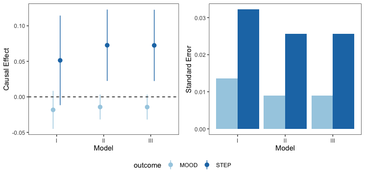
Figure 1: Causal effect point estimates with the 95% confidence interval, and standard errors

7.2 Time-varying treatment effect estimation

In most mobile health intervention studies, time-in-study has always been an important moderator of treatment effects. Therefore, for further investigation, we include study week in the marginal treatment effect model: $\beta(t)=\beta_{0}^{\star}+\beta_{1}^{\star}t$. Auxiliary variables are still chosen to be the corresponding outcome in the prior week. Control variables have been established in Section 7.1 as being beneficial in reducing standard errors, so control variables will always be included in the following analysis.

Estimated time-varying treatment moderation effects are shown in Figure 2 below. We compare our proposed approach against the WCLS method from Boruvka et al. (2018). More details of the moderated analysis are presented in Appendix L Table 9. The shaded area represents the 95% confidence band of the moderation effects at varying values of the moderator. A much narrower confidence band is observed when A2-WCLS is used; specifically, the relative efficiency for $\hat{\beta}_{0},\hat{\beta}_{1}$ in the mood model is 2.204 and 2.157, respectively, and in the step model is 1.562 and 1.475, respectively.

There is an overall decreasing trend of mood change with study week, which suggests that if the notifications don’t serve any therapeutic purposes, it might not be ideal to over-burden the participants with more targeted reminders, since it will bring down their mood. Furthermore, it is encouraging to see that the causal excursion effect of mobile prompts for step count change is positive in the first several weeks of the study, which means that sending targeted reminders is beneficial to increasing physical activity levels. In the later stages of the study, the effect fades away, possibly due to habituation to smartphone reminders.

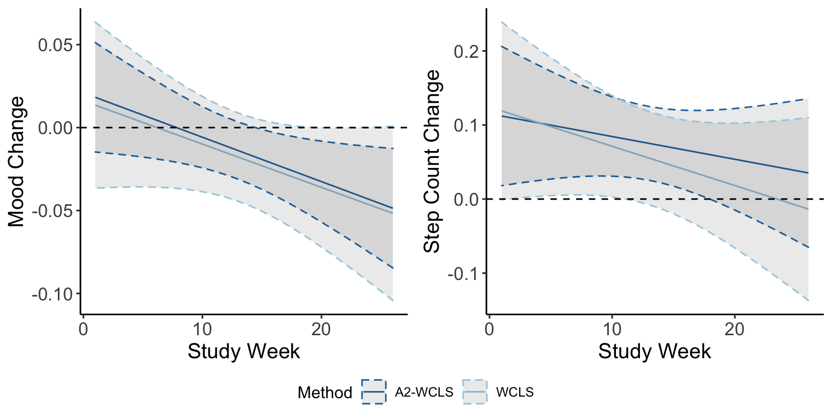
Figure 2: Causal effect point estimates with the 95% confidence interval, and standard errors

8 Discussion

MRTs are commonly used in mobile health-related studies, yet statistical techniques for covariate adjustment have mainly focused on RCTs with different sampling designs. In light of the increasing research on statistical tools for MRT analysis, we investigate the theoretical properties of incorporating auxiliary variables in the estimation of moderated causal excursion effects. Our study aims to address the current gaps in the literature by considering repeated measurements and time-varying treatment effects.

Our proposed A2-WCLS method possesses several desirable properties, such as computational simplicity, robustness to model misspecification, and wide applicability. Moreover, it provides valid statistical inference and demonstrates strong performance in finite-sample settings. Most importantly, it offers improved efficiency for moderated causal excursion effect estimation in comparison to the benchmark WCLS methods. In Appendix M, we provide clear and practical guidelines for practitioners to implement auxiliary variable adjustment in longitudinal studies. Overall, our results have the potential to alleviate confusion surrounding this topic and enhance the precision of causal effect estimation.

Many open questions remain. One of the most important is the choice of the centering function $\mu_{t}(S_{t})$, where we can use feature selection methods, such as the smooth clipped absolute deviation method (SCAD) Fan and Li (2001), to pick an optimal model for $\mu_{t}(S_{t})$. A non-linear centering function can also be considered, similar to Guo and Basse (2021) proposed for RCTs. In addition to using auxiliary variables to improve estimation efficiency, we may also consider adjusting for controlled variables $g(H_{t})$. There is a wide variety of machine learning methods that can be used for this purpose. Further, if the MRT establishes a certain type of cluster structure (interference within clusters and/or treatment heterogeneity at the cluster level), it definitely requires new centering techniques using cluster-level auxiliary variables (Shi et al., 2022). Last but not least, more advanced and flexible MRT designs should be explored and work in tandem with auxiliary variable adjustment to maximize efficiency, for example, Van Lancker et al. (2022) proposes using an information adaptive design, which adapts to the amount of precision gain and can lead to faster, more efficient trials, without sacrificing validity or power. We consider these to be exciting directions for future work.

Appendix A Proof of Lemma 3.2

A.1 Asymptotic Variance Comparison Between $\hat{\beta}_{0,t}^{\text{U}}$ and $\hat{\beta}_{0,t}^{\text{WCLS}}$

For the unadjusted estimator $\hat{\beta}_{0,t}^{\text{U}}$, the asymptotic variance can be consistently estimated by $Q_{t}^{-1}\Sigma_{t}^{\text{U}}Q_{t}^{-1}$:

$$\begin{split}Q_{t}&=p_{t}(1-p_{t})\\ \epsilon_{t}^{\text{U}}&=Y_{t+1}-\alpha_{0,t}-\left(A_{t}-p_{t}\right)\beta_{0,t}\\ \Sigma_{t}^{\text{U}}&=\mathbb{E}\Big{[}\left(\epsilon_{t}^{\text{U}}(A_{t}-p_{t})\right)^{2}\Big{]}\end{split}$$ (20)

For the WCLS estimator $\hat{\beta}_{0,t}^{\text{WCLS}}$, the asymptotic variance can be consistently estimated by $Q_{t}^{-1}\Sigma_{t}^{\text{WCLS}}Q_{t}^{-1}$:

$$\begin{split}Q_{t}&=p_{t}(1-p_{t})\\ \epsilon_{t}^{\text{WCLS}}&=Y_{t+1}-\alpha_{0,t}-\tilde{g}_{t}(H_{t})^{\top}\alpha_{1,t}-\left(A_{t}-p_{t}\right)\beta_{0,t}\\ \Sigma_{t}^{\text{WCLS}}&=\mathbb{E}\Big{[}\left(\epsilon_{t}^{\text{WCLS}}(A_{t}-p_{t})\right)^{2}\Big{]}\end{split}$$ (21)

For convenience, we center the control variables $g_{t}(H_{t})$ around their means, without loss of generality. Let $\tilde{g}_{t}(H_{t})$ represent the centered variables. To ensure clarity in the proof, we assume that $\tilde{g}_{t}(H_{t})^{\top}\alpha_{1,t}$ does not include the intercept term. Since the outer term $Q_{t}$ is the same for both asymptotic variance expressions, therefore, we only need to investigate the difference between $\Sigma_{t}^{\text{WCLS}}$ and $\Sigma_{t}^{\text{U}}$:

$$\Sigma_{t}^{\text{WCLS}} =\mathbb{E}\Big{[}\left((\epsilon_{t}^{\text{U}}-\tilde{g}_{t}(H_{t})^{\top}\alpha_{1,t})(A_{t}-p_{t})\right)^{2}\Big{]}$$

$$=\Sigma_{t}^{\text{U}}+\mathbb{E}\Big{[}\left(\tilde{g}_{t}(H_{t})^{\top}\alpha_{1,t}(A_{t}-p_{t})\right)^{2}\Big{]}-2\mathbb{E}\Big{[}\epsilon_{t}^{\text{U}}\tilde{g}_{t}(H_{t})^{\top}\alpha_{1,t}(A_{t}-p_{t})^{2}\Big{]}$$

The expansion shows that the difference between $\Sigma_{t}^{\text{WCLS}}$ and $\Sigma_{t}^{\text{U}}$ is:

$$\mathbb{E}\Big{[}\left(\tilde{g}_{t}(H_{t})^{\top}\alpha_{1,t}(A_{t}-p_{t})\right)^{2}\Big{]}-2\mathbb{E}\Big{[}\epsilon_{t}^{\text{U}}\tilde{g}_{t}(H_{t})^{\top}\alpha_{1,t}(A_{t}-p_{t})^{2}\Big{]}$$ (22)

The first quadratic term is given by:

$$\mathbb{E}\Big{[}(A_{t}-p_{t})^{2}\alpha_{1,t}^{\top}\tilde{g}_{t}(H_{t})\tilde{g}_{t}(H_{t})^{\top}\alpha_{1,t}\Big{]}=p_{t}(1-p_{t})\alpha_{1,t}^{\top}\Sigma(g_{t}(H_{t}))\alpha_{1,t}$$

where $\Sigma(g_{t}(H_{t}))=\mathbb{E}\Big{[}\tilde{g}_{t}(H_{t})\tilde{g}_{t}(H_{t})^{\top}\Big{]}\in\mathbb{R}^{d\times d}$ represents the variance-covariance matrix for the control variables $g_{t}(H_{t})$. The second interaction term could be further simplified as:

$$\mathbb{E}\Big{[}\epsilon_{t}^{\text{U}}\tilde{g}_{t}(H_{t})^{\top}\alpha_{1,t}(A_{t}-p_{t})^{2}\Big{]}$$

$$= \mathbb{E}\Big{[}\left(\mathbb{E}[\epsilon_{t}^{\text{U}}|A_{t}=1,H_{t}]p_{t}(1-p_{t})^{2}+\mathbb{E}[\epsilon_{t}^{\text{U}}|A_{t}=0,H_{t}]p_{t}^{2}(1-p_{t})\right)\tilde{g}_{t}(H_{t})^{\top}\alpha_{1,t}\Big{]}$$

$$= p_{t}(1-p_{t})\mathbb{E}\Big{[}\left(\mathbb{E}[\epsilon_{t}^{\text{U}}|A_{t}=1,H_{t}](1-p_{t})+E[\epsilon_{t}^{\text{U}}|A_{t}=0,H_{t}]p_{t}\right)\tilde{g}_{t}(H_{t})^{\top}\alpha_{1,t}\Big{]}$$

$$= p_{t}(1-p_{t})\bigg{(}\mathbb{E}\Big{[}\mathbb{E}[\epsilon_{t}^{\text{U}}|A_{t}=1,H_{t}]\tilde{g}_{t}(H_{t})^{\top}\alpha_{1,t}\Big{]}$$

$$- p_{t}\mathbb{E}\Big{[}(\mathbb{E}[\epsilon_{t}^{\text{U}}|A_{t}=1,H_{t}]-\mathbb{E}[\epsilon_{t}^{\text{U}}|A_{t}=0,H_{t}])\tilde{g}_{t}(H_{t})^{\top}\alpha_{1,t}\Big{]}\bigg{)}.$$

It rests to study the following term:

$$\mathbb{E}\Big{[}\mathbb{E}[\epsilon_{t}^{\text{U}}|A_{t}=1,H_{t}]\tilde{g}_{t}(H_{t})^{\top}\Big{]}$$

$$= \mathbb{E}\Big{[}\mathbb{E}[Y_{t+1}-(1-p_{t})\beta_{0,t}|A_{t}=1,H_{t}]\tilde{g}_{t}(H_{t})^{\top}\Big{]}$$

$$= \mathbb{E}\Big{[}\mathbb{E}[Y_{t+1}|A_{t}=1,H_{t}]\tilde{g}_{t}(H_{t})^{\top}\Big{]}$$

$$= \mathbb{E}\Big{[}(\mathbb{E}[Y_{t+1}|A_{t}=1,H_{t}]-\mathbb{E}[Y_{t+1}|H_{t}]+\mathbb{E}[Y_{t+1}|H_{t}])\tilde{g}_{t}(H_{t})^{\top}\Big{]}$$

$$= \mathbb{E}\Big{[}(\mathbb{E}[Y_{t+1}|A_{t}=1,H_{t}]-\mathbb{E}[Y_{t+1}|H_{t}])\tilde{g}_{t}(H_{t})^{\top}\Big{]}+\alpha_{1,t}^{\top}\Sigma(g_{t}(H_{t}))$$

$$= (1-p_{t})\beta_{1,t}^{\top}\Sigma(g_{t}(H_{t}))+\alpha_{1,t}^{\top}\Sigma(g_{t}(H_{t})),$$

and similarly

$$\mathbb{E}\Big{[}\mathbb{E}[\epsilon_{t}^{\text{U}}|A_{t}=0,H_{t}]\tilde{g}_{t}(H_{t})^{\top}\Big{]}=-p_{t}\beta_{1,t}^{\top}\Sigma(g_{t}(H_{t}))+\alpha_{1,t}^{\top}\Sigma(g_{t}(H_{t}))$$

Then combing these two terms together, we have:

$$\Sigma_{t}^{\text{WCLS}}-\Sigma_{t}^{\text{U}} =-p_{t}(1-p_{t})\alpha_{1,t}^{\top}\Sigma(g_{t}(H_{t}))\left(\alpha_{1,t}+2(1-2p_{t})\beta_{1,t}\right)$$ (23)

Appendix B Proof of Lemma 3.3

B.1 Asymptotic Properties of $\hat{\beta}_{0,t}^{\text{L}}$

As per Lin (2013); Boruvka et al. (2018), $\hat{\beta}_{0,t}^{\text{L}}$ obtained by minimizing (7) is consistent and asymptotically normal. We proceed with the proof by centering $g_{t}(H_{t})$ at its mean and denoting it as $\tilde{g}_{t}(H_{t})$. And the asymptotic variance can be consistently estimated by $Q_{t}^{-1}\Sigma_{t}^{\text{L}}Q_{t}^{-1}$, where

$$\begin{split}Q_{t}&=p_{t}(1-p_{t})\\ \epsilon_{t}^{\text{L}}&=Y_{t+1}-\alpha_{0,t}-\tilde{g}_{t}(H_{t})^{\top}\alpha_{1,t}-\left(A_{t}-p_{t}\right)(\beta_{0,t}+\tilde{g}_{t}(H_{t})\beta_{1,t})\\ \Sigma_{t}^{\text{L}}&=\mathbb{E}\Big{[}\left(\epsilon_{t}^{\text{L}}(A_{t}-p_{t})\right)^{2}\Big{]}\end{split}$$ (24)

B.2 Asymptotic Variance Comparison Between $\hat{\beta}_{0,t}^{\text{L}}$ and $\hat{\beta}_{0,t}^{\text{U}}$

Since the outer term $Q_{t}$ is the same for both asymptotic variance expressions, therefore, we only need to investigate the difference between $\Sigma_{t}^{\text{L}}$ and $\Sigma_{t}^{\text{U}}$.

$$\Sigma_{t}^{\text{L}} =\mathbb{E}\Big{[}\left((\epsilon_{t}^{\text{U}}-\tilde{g}_{t}(H_{t})^{\top}\alpha_{1,t}-(A_{t}-p_{t})\tilde{g}_{t}(H_{t})^{\top}\beta_{1,t})(A_{t}-p_{t})\right)^{2}\Big{]}$$

$$=\Sigma_{t}^{\text{U}}+\mathbb{E}\Big{[}\left(\tilde{g}_{t}(H_{t})^{\top}\alpha_{1,t}+(A_{t}-p_{t})\tilde{g}_{t}(H_{t})^{\top}\beta_{1,t}\right)^{2}(A_{t}-p_{t})^{2}\Big{]}$$

$$-2\mathbb{E}\Big{[}\epsilon_{t}^{\text{U}}(\tilde{g}_{t}(H_{t})^{\top}\alpha_{1,t}+(A_{t}-p_{t})\tilde{g}_{t}(H_{t})^{\top}\beta_{1,t})(A_{t}-p_{t})^{2}\Big{]}$$

The expansion shows that the difference between $\Sigma_{t}^{\text{L}}$ and $\Sigma_{t}^{\text{U}}$ is:

$$\begin{split}&\mathbb{E}\Big{[}\left(\tilde{g}_{t}(H_{t})^{\top}\alpha_{1,t}+(A_{t}-p_{t})\tilde{g}_{t}(H_{t})^{\top}\beta_{1,t}\right)^{2}(A_{t}-p_{t})^{2}\Big{]}\\ &-2\mathbb{E}\Big{[}\epsilon_{t}^{\text{U}}(\tilde{g}_{t}(H_{t})^{\top}\alpha_{1,t}+(A_{t}-p_{t})\tilde{g}_{t}(H_{t})^{\top}\beta_{1,t})(A_{t}-p_{t})^{2}\Big{]}\end{split}$$ (25)

The first quadratic term is given by:

$$\mathbb{E}\Big{[}\left(\tilde{g}_{t}(H_{t})^{\top}\alpha_{1,t}+(A_{t}-p_{t})\tilde{g}_{t}(H_{t})^{\top}\beta_{1,t}\right)^{2}(A_{t}-p_{t})^{2}\Big{]}$$

$$= p_{t}(1-p_{t})\Big{[}\alpha_{1,t}^{\top}\Sigma(g_{t}(H_{t}))\alpha_{1,t}+2(1-2p_{t})\alpha_{1,t}^{\top}\Sigma(g_{t}(H_{t}))\beta_{1,t}+(1-3p_{t}+3p_{t}^{2})\beta_{1,t}^{\top}\Sigma(g_{t}(H_{t}))\beta_{1,t}\Big{]}$$

The second interaction term could be further simplified as:

$$\mathbb{E}\Big{[}\epsilon_{t}^{\text{U}}(\tilde{g}_{t}(H_{t})^{\top}\alpha_{1,t}+(A_{t}-p_{t})\tilde{g}_{t}(H_{t})^{\top}\beta_{1,t})(A_{t}-p_{t})^{2}\Big{]}$$

$$= \mathbb{E}\Big{[}\left(\mathbb{E}[\epsilon_{t}^{\text{U}}|A_{t}=1,H_{t}]p_{t}(1-p_{t})^{2}+\mathbb{E}[\epsilon_{t}^{\text{U}}|A_{t}=0,H_{t}]p_{t}^{2}(1-p_{t})\right)\tilde{g}_{t}(H_{t})^{\top}\alpha_{1,t}\Big{]}$$

$$+\mathbb{E}\Big{[}\left(\mathbb{E}[\epsilon_{t}^{\text{U}}|A_{t}=1,H_{t}]p_{t}(1-p_{t})^{3}-\mathbb{E}[\epsilon_{t}^{\text{U}}|A_{t}=0,H_{t}]p_{t}^{3}(1-p_{t})\right)\tilde{g}_{t}(H_{t})^{\top}\beta_{1,t}\Big{]}$$

$$= p_{t}(1-p_{t})\mathbb{E}\Big{[}\left(\mathbb{E}[\epsilon_{t}^{\text{U}}|A_{t}=1,H_{t}](1-p_{t})+\mathbb{E}[\epsilon_{t}^{\text{U}}|A_{t}=0,H_{t}]p_{t}\right)\tilde{g}_{t}(H_{t})^{\top}\alpha_{1,t}\Big{]}$$

$$+p_{t}(1-p_{t})\mathbb{E}\Big{[}\left(\mathbb{E}[\epsilon_{t}^{\text{U}}|A_{t}=1,H_{t}](1-p_{t})^{2}-\mathbb{E}[\epsilon_{t}^{\text{U}}|A_{t}=0,H_{t}]p^{2}_{t}\right)\tilde{g}_{t}(H_{t})^{\top}\beta_{1,t}\Big{]}$$

Recall:

$$\mathbb{E}\Big{[}\mathbb{E}[\epsilon_{t}^{\text{U}}|A_{t}=1,H_{t}]\tilde{g}_{t}(H_{t})^{\top}\Big{]} =(1-p_{t})\beta_{1,t}^{\top}\Sigma(g_{t}(H_{t}))+\alpha_{1,t}^{\top}\Sigma(g_{t}(H_{t}))$$

$$\mathbb{E}\Big{[}\mathbb{E}[\epsilon_{t}^{\text{U}}|A_{t}=0,H_{t}]\tilde{g}_{t}(H_{t})^{\top}\Big{]} =-p_{t}\beta_{1,t}^{\top}\Sigma(g_{t}(H_{t}))+\alpha_{1,t}^{\top}\Sigma(g_{t}(H_{t}))$$

Then combing these two terms together, we have $\Sigma_{t}^{\text{L}}-\Sigma_{t}^{\text{U}}$ equals to:

$$-p_{t}(1-p_{t})\Big{[}\left(\alpha_{1,t}+(1-2p_{t})\beta_{1,t}\right)^{\top}\Sigma(g_{t}(H_{t}))\left(\alpha_{1,t}+(1-2p_{t})\beta_{1,t}\right)+p_{t}(1-p_{t})\beta_{1,t}^{\top}\Sigma(g_{t}(H_{t}))\beta_{1,t}\Big{]},$$ (26)

which is guaranteed to be non-positive.

B.3 Efficiency Comparison Between $\hat{\beta}_{0,t}^{\text{L}}$ and $\hat{\beta}_{0,t}^{\text{WCLS}}$

Simply applying the differences derived above, namely (23) and (26), we can easily get the asymptotic variance difference:

$$\Sigma_{t}^{\text{L}}-\Sigma_{t}^{\text{WCLS}}=-p_{t}(1-p_{t})\Big{[}(1-3p_{t}+3p_{t}^{2})\beta_{1,t}^{\top}\Sigma(g_{t}(H_{t}))\beta_{1,t}\Big{]},$$ (27)

which is guaranteed to be non-positive.

Appendix C Proof of Condition 3.5

To illustrate the derivation of the orthogonality condition in detail, we write down the derivatives of (10) and (3) with respect to $\beta_{0}$. The derivative of (3) with respect to $\beta_{0}$ is:

$$\mathbb{E}\left[\sum_{t=1}^{T}W_{t}(Y_{t+1}-g_{t}(H_{t})^{\top}\alpha-(A_{t}-\tilde{p}_{t})f_{t}(S_{t})^{\top}\beta_{0})(A_{t}-\tilde{p}_{t})f_{t}(S_{t})\right]$$ (28)

The derivative of (10) with respect to $\beta_{0}$ is:

$$\mathbb{E}\left[\sum_{t=1}^{T}W_{t}(Y_{t+1}-g_{t}(H_{t})^{\top}\alpha-(A_{t}-\tilde{p}_{t})(f_{t}(S_{t})^{\top}\beta_{0}+(Z_{t}-\mu_{t}(S_{t}))^{\top}\beta_{1}))(A_{t}-\tilde{p}_{t})f_{t}(S_{t})\right]$$ (29)

The intuition is that if the difference between (28) and (29) is always zero (not depending on the form of $\mu_{t}(S_{t})$), then both of them should have the same minimizer for $\beta_{0}$:

$$\mathbb{E}\left[\sum_{t=1}^{T}W_{t}(A_{t}-\tilde{p}_{t})^{2}f_{t}(S_{t})(Z_{t}-\mu_{t}(S_{t}))^{\top}\beta_{1}\right]=\mathbf{0}_{q\times 1}$$

After calculating the expectation of the term above, we can obtain the form of orthogonality constraint shown in Condition 3.5. For each $Z^{i}_{t}-\mu^{i}_{t}(S_{t})$ we wish to include:

$$\mathbb{E}\left[\sum_{t=1}^{T}\tilde{p}_{t}(1-\tilde{p}_{t})f_{t}(S_{t})(Z^{i}_{t}-\mu^{i}_{t}(S_{t}))^{\top}\right]=\mathbf{0}_{q\times 1}$$

C.1 Neyman Orthogonality

We are interested in the true value $\beta_{0}^{\star}$ of the low-dimensional target parameter $\beta_{0}$. Therefore in the estimation procedure, $\beta_{1}$ and $\alpha$ are treated as nuisance parameters. First, we assume that $\beta_{0}^{\star}$ satisfies the moment conditions:

$$\mathbb{E}[\psi(\beta_{0}^{\star};\beta_{1}^{\star},\alpha^{\star})]=0$$

where $\psi(\beta_{0};\beta_{1},\alpha)$ is a known score function. In our case, $\psi(\beta_{0};\beta_{1},\alpha)$ is exactly the estimating equation for $\beta_{0}$:

$$\sum_{t=1}^{T}W_{t}\Big{[}Y_{t+1}-g_{t}(H_{t})^{\top}\alpha-(A_{t}-\tilde{p}_{t})(f_{t}(S_{t})^{\top}\beta_{0}+(Z_{t}-\mu_{t}(S_{t}))^{\top}\beta_{1})\Big{]}(A_{t}-\tilde{p}_{t})f_{t}(S_{t})$$

Here we further require the Neyman orthogonality condition for the score $\psi$. By the definition given in Chernozhukov et al. (2018), the Gateaux derivative operator with respect to $\beta_{1}$ is:

$$G(\beta_{1})=\mathbb{E}\left[\sum_{t=1}^{T}W_{t}(A_{t}-\tilde{p}_{t})^{2}f_{t}(S_{t})(Z_{t}-\mu_{t}(S_{t}))^{\top}\right](\beta_{1}-\beta_{1,0})$$

which should vanish when evaluated at the true parameter values $\beta_{1,0}=\beta_{1}^{\star}$, which implies that:

$$\mathbb{E}\left[\sum_{t=1}^{T}\tilde{p}_{t}(1-\tilde{p}_{t})f_{t}(S_{t})(Z_{t}-\mu_{t}(S_{t}))^{\top}\right]=\mathbf{0}_{q\times p}$$

Similarly, we can obtain the form of orthogonality constraint shown in Condition 3.5.

Appendix D Proof of Lemma 3.6

The A2-WCLS criterion is:

$$\mathbb{P}_{n}\left[\sum_{t=1}^{T}W_{t}\times\left(Y_{t+1}-g_{t}(H_{t})^{\top}\alpha-\left(A_{t}-\tilde{p}_{t}(1\mid S_{t})\right)(f_{t}(S_{t})^{\top}\beta_{0}+(Z_{t}-\mu_{t}(S_{t}))^{\top}\beta_{1})\right)^{2}\right]$$

which can be expressed as the following estimating equation:

$$U(\alpha,\beta_{0},\beta_{1};\mu_{t})=\mathbb{E}\Bigg{[}\sum_{t=1}^{T}W_{t}(Y_{t+1}-g_{t}(H_{t})^{\top}\alpha- (A_{t}-\tilde{p}_{t})(f_{t}(S_{t})^{\top}\beta_{0}+(Z_{t}-\mu_{t}(S_{t}))^{\top}\beta_{1}))$$

$$\times\left(\begin{array}[]{c}g_{t}(H_{t})\\ (A_{t}-\tilde{p}_{t})f_{t}(S_{t})\\ (A_{t}-\tilde{p}_{t})(Z_{t}-\mu_{t}(S_{t}))\end{array}\right)\Bigg{]}$$ (33)

Assuming the centering functions $\mu_{t}(S_{t})$ satisfy the orthogonality condition 3.5, then we have:

$$\mathbb{E}\left[\sum_{t=1}^{T}W_{t}(Y_{t+1}-g_{t}(H_{t})^{\top}\alpha-(A_{t}-\tilde{p}_{t})(f_{t}(S_{t})^{\top}\beta_{0}+(Z_{t}-\mu_{t}(S_{t}))^{\top}\beta_{1}))(A_{t}-\tilde{p}_{t})f_{t}(S_{t})\right]$$

$$= \mathbb{E}\left[\sum_{t=1}^{T}W_{t}(Y_{t+1}-g_{t}(H_{t})^{\top}\alpha-(A_{t}-\tilde{p}_{t})f_{t}(S_{t})^{\top}\beta_{0})(A_{t}-\tilde{p}_{t})f_{t}(S_{t})\right]$$

$$-\mathbb{E}\left[\sum_{t=1}^{T}W_{t}(A_{t}-\tilde{p}_{t})^{2}f_{t}(S_{t})(Z_{t}-\mu_{t}(S_{t}))^{\top}\right]\beta_{1}~{}~{}~{}~{}\text{(orthogonality condition)}$$

$$= \mathbb{E}\left[\sum_{t=1}^{T}W_{t}(Y_{t+1}-g_{t}(H_{t})^{\top}\alpha-(A_{t}-\tilde{p}_{t})f_{t}(S_{t})^{\top}\beta_{0})(A_{t}-\tilde{p}_{t})f_{t}(S_{t})\right]~{}~{}~{}~{}~{}\text{(WCLS estimating equation)}$$

Based on the asymptotic properties proved in Boruvka et al. (2018), $\hat{\beta}_{0}^{\text{A2}}$ is consistent and asymptotically normal, and the robust sandwich variance-covariance estimator is applied here to consistently estimate the asymptotic variance of $\hat{\beta}_{0}^{\text{A2}}$, which can be retrieved from the middle block diagonal $(q\times q)$ matrix:

$$Q^{-1}\Sigma Q^{-1}=\mathbb{E}\left[\dot{U}(\alpha,\beta_{0},\beta_{1};\mu_{t})\right]^{-1}\mathbb{E}\left[U(\alpha,\beta_{0},\beta_{1};\mu_{t})\right]^{\otimes 2}\mathbb{E}\left[\dot{U}(\alpha,\beta_{0},\beta_{1};\mu_{t})\right]^{-1}$$

Specifically, for the WCLS criterion:

$$\begin{split}Q&=\mathbb{E}\left[\sum_{t=1}^{T}\tilde{p}_{t}(1-\tilde{p}_{t})f_{t}(S_{t})f_{t}(S_{t})^{\top}\right],\\ \epsilon_{t}^{\text{WCLS}}&=Y_{t+1}-g_{t}(H_{t})^{\top}\alpha-\left(A_{t}-\tilde{p}_{t}\right)f_{t}(S_{t})^{\top}\beta_{0},\\ \Sigma^{\text{WCLS}}&=\mathbb{E}\left[\left(\sum_{t=1}^{T}W_{t}\epsilon_{t}^{\text{WCLS}}(A_{t}-\tilde{p}_{t})f_{t}(S_{t})\right)\left(\sum_{t=1}^{T}W_{t}\epsilon_{t}^{\text{WCLS}}(A_{t}-\tilde{p}_{t})f_{t}(S_{t})\right)^{\top}\right].\end{split}$$ (34)

For the A2-WCLS criterion:

$$\begin{split}Q&=\mathbb{E}\left[\sum_{t=1}^{T}\tilde{p}_{t}(1-\tilde{p}_{t})f_{t}(S_{t})f_{t}(S_{t})^{\top}\right],\\ \epsilon_{t}^{\text{A2}}&=Y_{t+1}-g_{t}(H_{t})^{\top}\alpha-\left(A_{t}-\tilde{p}_{t}\right)(f_{t}(S_{t})^{\top}\beta_{0}+(Z_{t}-\mu_{t}(S_{t}))^{\top}\beta_{1}),\\ \Sigma^{\text{A2}}&=\mathbb{E}\left[\left(\sum_{t=1}^{T}W_{t}\epsilon_{t}^{\text{A2}}(A_{t}-\tilde{p}_{t})f_{t}(S_{t})\right)\left(\sum_{t=1}^{T}W_{t}\epsilon_{t}^{\text{A2}}(A_{t}-\tilde{p}_{t})f_{t}(S_{t})\right)^{\top}\right].\end{split}$$ (35)

Appendix E Proof of Lemma 3.8

The relationship between two residuals $\epsilon_{t}^{\text{A2}}$ and $\epsilon_{t}^{\text{WCLS}}$ is:

$$\epsilon_{t}^{\text{A2}}=\epsilon_{t}^{\text{WCLS}}-(A_{t}-\tilde{p}_{t})(Z_{t}-\mu_{t}(S_{t}))^{\top}\beta_{1}$$

Thus, the estimating equation for parameter $\beta_{1}$ from the A2-WCLS criterion can be written as:

$$0=\mathbb{E}\left[\sum_{t=1}^{T}W_{t}(\epsilon_{t}^{\text{WCLS}}-(A_{t}-\tilde{p}_{t})(Z_{t}-\mu_{t}(S_{t}))^{\top}\beta_{1})(A_{t}-\tilde{p}_{t})(Z_{t}-\mu_{t}(S_{t}))\right]$$

Solving the equation above, we have:

$$\beta_{1}^{\star}(\mu_{t}(S_{t}))=\mathbb{E}\left[\sum_{t=1}^{T}\tilde{p}_{t}(1-\tilde{p}_{t})\Sigma_{\mu}(S_{t})\right]^{-1}\mathbb{E}\left[\sum_{t=1}^{T}\tilde{p}_{t}(1-\tilde{p}_{t})(\beta(t;Z_{t},S_{t})-\beta(t;S_{t}))(Z_{t}-\mu_{t}(S_{t}))\right]$$ (36)

where $\Sigma_{\mu}(Z_{t})=\mathbb{E}[(Z_{t}-\mu_{t}(S_{t}))(Z_{t}-\mu_{t}(S_{t}))^{\top}]$. For the first property, if $Z_{t}$ is in fact not a moderator, then $\beta(t;Z_{t},S_{t})-\beta(t;S_{t})=0$ for every $t$. Plug in Equation (36), we have $\beta_{1}^{\star}=0$. For the second property, we can demonstrate that the first term of $\beta_{1}^{\star}(\mu_{t}(S_{t}))$ is less than or equal to that of $\beta_{1}^{\star}$:

$$\mathbb{E}\left[\sum_{t=1}^{T}\tilde{p}_{t}(1-\tilde{p}_{t})\Big{(}Z_{t}-\mathbb{E}[Z_{t}|S_{t}]+\mathbb{E}[Z_{t}|S_{t}]-\mu_{t}(S_{t})\Big{)}\Big{(}Z_{t}-\mathbb{E}[Z_{t}|S_{t}]+\mathbb{E}[Z_{t}|S_{t}]-\mu_{t}(S_{t})\Big{)}^{\top}\right]^{-1}$$

$$\leq \mathbb{E}\left[\sum_{t=1}^{T}\tilde{p}_{t}(1-\tilde{p}_{t})\Big{(}Z_{t}-\mathbb{E}[Z_{t}|S_{t}]\Big{)}\Big{(}Z_{t}-\mathbb{E}[Z_{t}|S_{t}]\Big{)}^{\top}\right]^{-1}$$

and the second terms are equal:

$$\mathbb{E}\left[\sum_{t=1}^{T}\tilde{p}_{t}(1-\tilde{p}_{t})\mathbb{E}[(\beta(t;Z_{t},S_{t})-\beta(t;S_{t}))(Z_{t}-\mu_{t}(S_{t}))]\right]$$

$$= \mathbb{E}\left[\sum_{t=1}^{T}\tilde{p}_{t}(1-\tilde{p}_{t})(\beta(t;Z_{t},S_{t})-\beta(t;S_{t}))(Z_{t}-\mathbb{E}[Z_{t}|S_{t}])\right]$$

Therefore, $|\beta_{1}^{\star}(\mu_{t})|\leq|\beta_{1}(\mathbb{E}[Z_{t}|S_{t}])|$, which means that $\beta_{1}^{\star}(\mu_{t})$ underestimates the true moderation effect.

Appendix F Proof of Theorem 4.2

Recall the asymptotic variance expressions presented in (34) and (35), the outer term $Q$ is the same for both, therefore, we only need to investigate the difference between $\Sigma^{\text{A2}}$ and $\Sigma^{\text{WCLS}}$. And it’s easy to see that $\Sigma^{\text{WCLS}}$ can be expanded as below:

$$\Sigma^{\text{WCLS}} =\mathbb{E}\left[\left(\sum_{t=1}^{T}W_{t}\epsilon_{t}^{\text{A2}}(A_{t}-\tilde{p}_{t})f_{t}(S_{t})\right)\left(\sum_{t=1}^{T}W_{t}\epsilon_{t}^{\text{A2}}(A_{t}-\tilde{p}_{t})f_{t}(S_{t})\right)^{\top}\right]$$

$$+2\mathbb{E}\Bigg{[}\sum_{t,t^{\prime}=1}^{T}W_{t}\epsilon_{t}^{\text{A2}}(A_{t}-\tilde{p}_{t})f_{t}(S_{t})\times W_{t^{\prime}}(A_{t^{\prime}}-\tilde{p}_{t^{\prime}})^{2}(Z_{t^{\prime}}-\mu_{t^{\prime}}(S_{t^{\prime}}))^{\top}\beta_{1}f_{t^{\prime}}(S_{t^{\prime}})^{\top}\Bigg{]}$$

$$+\mathbb{E}\left[\left(\sum_{t=1}^{T}W_{t}(A_{t}-\tilde{p}_{t})^{2}(Z_{t}-\mu_{t}(S_{t}))^{\top}\beta_{1}f_{t}(S_{t})\right)\left(\sum_{t=1}^{T}W_{t}(A_{t}-\tilde{p}_{t})^{2}(Z_{t}-\mu_{t}(S_{t}))^{\top}\beta_{1}f_{t}(S_{t})\right)^{\top}\right].$$

The expansion shows that the difference between $\Sigma^{\text{A2}}$ and $\Sigma^{\text{WCLS}}$ is:

$$- 2\mathbb{E}\Bigg{[}\sum_{t,t^{\prime}=1}^{T}W_{t}\epsilon_{t}^{\text{A2}}(A_{t}-\tilde{p}_{t})f_{t}(S_{t})\times W_{t^{\prime}}(A_{t^{\prime}}-\tilde{p}_{t^{\prime}})^{2}(Z_{t^{\prime}}-\mu_{t^{\prime}}(S_{t^{\prime}}))^{\top}\beta_{1}f_{t^{\prime}}(S_{t^{\prime}})^{\top}\Bigg{]}$$

$$- \mathbb{E}\left[\left(\sum_{t=1}^{T}W_{t}(A_{t}-\tilde{p}_{t})^{2}(Z_{t}-\mu_{t}(S_{t}))^{\top}\beta_{1}f_{t}(S_{t})\right)\left(\sum_{t=1}^{T}W_{t}(A_{t}-\tilde{p}_{t})^{2}(Z_{t}-\mu_{t}(S_{t}))^{\top}\beta_{1}f_{t}(S_{t})\right)^{\top}\right]$$

Under the assumption that the true causal excursion effect $\beta_{t}(t;H_{t})$ is correctly specified by the linear model:

$$\beta(t;H_{t})=f_{t}(S_{t})^{\top}\beta_{0}+(Z_{t}-\mu_{t}(S_{t}))^{\top}\beta_{1}$$

which equivalent to:

$$\mathbb{E}\left[\epsilon_{t}^{\text{A2}}|H_{t},1\right]-\mathbb{E}\left[\epsilon_{t}^{\text{A2}}|H_{t},0\right]$$

$$= \mathbb{E}\left[Y_{t+1}|H_{t},1\right]-\mathbb{E}\left[Y_{t+1}|H_{t},0\right]-f_{t}(S_{t})^{\top}\beta_{0}-(Z_{t}-\mu_{t}(S_{t}))^{\top}\beta_{1}$$

$$= 0$$

We first study the interaction term with $t>t^{\prime}$:

$$\mathbb{E}\Bigg{[}W_{t}\epsilon_{t}^{\text{A2}}(A_{t}-\tilde{p}_{t})f_{t}(S_{t})\times W_{t^{\prime}}(A_{t^{\prime}}-\tilde{p}_{t^{\prime}})^{2}(Z_{t^{\prime}}-\mu_{t^{\prime}}(S_{t^{\prime}}))^{\top}\beta_{1}f_{t^{\prime}}(S_{t^{\prime}})^{\top}\Bigg{]}$$

$$= \mathbb{E}\Bigg{[}\mathbb{E}\left[W_{t}\epsilon_{t}^{\text{A2}}(A_{t}-\tilde{p}_{t})|H_{t}\right]f_{t}(S_{t})\times W_{t^{\prime}}(A_{t^{\prime}}-\tilde{p}_{t^{\prime}})^{2}(Z_{t^{\prime}}-\mu_{t^{\prime}}(S_{t^{\prime}}))^{\top}\beta_{1}f_{t^{\prime}}(S_{t^{\prime}})^{\top}\Bigg{]}$$

$$= \mathbb{E}\Bigg{[}\tilde{p}_{t}(1-\tilde{p}_{t})\underbrace{\Big{(}\mathbb{E}\left[\epsilon_{t}^{\text{A2}}|H_{t},1\right]-\mathbb{E}\left[\epsilon_{t}^{\text{A2}}|H_{t},0\right]\Big{)}}_{=0}f_{t}(S_{t})\times W_{t^{\prime}}(A_{t^{\prime}}-\tilde{p}_{t^{\prime}})^{2}(Z_{t^{\prime}}-\mu_{t^{\prime}}(S_{t^{\prime}}))^{\top}\beta_{1}f_{t^{\prime}}(S_{t^{\prime}})^{\top}\Bigg{]}$$

$$= 0$$

Besides, for terms with $t<t^{\prime}$:

$$\mathbb{E}\Bigg{[}W_{t}\epsilon_{t}^{\text{A2}}(A_{t}-\tilde{p}_{t})f_{t}(S_{t})\times W_{t^{\prime}}(A_{t^{\prime}}-\tilde{p}_{t^{\prime}})^{2}(Z_{t^{\prime}}-\mu_{t^{\prime}}(S_{t^{\prime}}))^{\top}\beta_{1}f_{t^{\prime}}(S_{t^{\prime}})^{\top}\Bigg{]}$$

$$= \mathbb{E}\Bigg{[}W_{t}\epsilon_{t}^{\text{A2}}(A_{t}-\tilde{p}_{t})f_{t}(S_{t})\times\mathbb{E}\Big{[}W_{t^{\prime}}(A_{t^{\prime}}-\tilde{p}_{t^{\prime}})^{2}|H_{t^{\prime}}\Big{]}(Z_{t^{\prime}}-\mu_{t^{\prime}}(S_{t^{\prime}}))^{\top}\beta_{1}f_{t^{\prime}}(S_{t^{\prime}})^{\top}\Bigg{]}$$

$$= \mathbb{E}\Bigg{[}W_{t}\epsilon_{t}^{\text{A2}}(A_{t}-\tilde{p}_{t})f_{t}(S_{t})\times\tilde{p}_{t^{\prime}}(1-\tilde{p}_{t^{\prime}})(Z_{t^{\prime}}-\mu_{t^{\prime}}(S_{t^{\prime}}))^{\top}\beta_{1}f_{t^{\prime}}(S_{t^{\prime}})^{\top}\Bigg{]}$$

$$= \mathbb{E}\Bigg{[}W_{t}(A_{t}-\tilde{p}_{t})f_{t}(S_{t})\underbrace{\mathbb{E}\Big{[}\epsilon_{t}^{\text{A2}}\times\tilde{p}_{t^{\prime}}(1-\tilde{p}_{t^{\prime}})(Z_{t^{\prime}}-\mu_{t^{\prime}}(S_{t^{\prime}}))^{\top}\beta_{1}f_{t^{\prime}}(S_{t^{\prime}})^{\top}|H_{t},A_{t}\Big{]}}_{=0}\Bigg{]}$$

$$= 0$$

The last step invokes the conditionally uncorrelated assumption, saying that the $\epsilon_{t}^{\text{A2}}$ is uncorrelated to future $Z_{t^{\prime}}$ and $f_{t^{\prime}}(S_{t^{\prime}})$. As for $t=t^{\prime}$:

$$\mathbb{E}\Bigg{[}W_{t}^{2}\epsilon_{t}^{\text{A2}}(A_{t}-\tilde{p}_{t})f_{t}(S_{t})\times(A_{t}-\tilde{p}_{t})^{2}(Z_{t}-\mu_{t}(S_{t}))^{\top}\beta_{1}f_{t}(S_{t})^{\top}\Bigg{]}$$

$$= \mathbb{E}\Bigg{[}W_{t}^{2}\epsilon_{t}^{\text{A2}}(A_{t}-\tilde{p}_{t})^{3}(Z_{t}-\mu_{t}(S_{t}))^{\top}\beta_{1}f_{t}(S_{t})f_{t}(S_{t})^{\top}\Bigg{]}$$

$$= \mathbb{E}\Bigg{[}\tilde{p}^{3}_{t}(1-\tilde{p}_{t})^{3}\Big{(}\frac{1}{p_{t}(1|H_{t})}\mathbb{E}\Big{[}\epsilon_{t}^{\text{A2}}|H_{t},A_{t}=1\Big{]}-\frac{1}{p_{t}(0|H_{t})}\mathbb{E}\Big{[}\epsilon_{t}^{\text{A2}}|H_{t},A_{t}=0\Big{]}\Big{)}(Z_{t}-\mu_{t}(S_{t}))^{\top}\beta_{1}f_{t}(S_{t})f_{t}(S_{t})^{\top}\Bigg{]}$$

it rests on studying the following terms:

$$\mathbb{E}\Big{[}\epsilon_{t}^{\text{A2}}|H_{t},A_{t}=1\Big{]}(Z_{t}-\mu_{t}(S_{t}))^{\top}$$

$$= \mathbb{E}\Big{[}Y_{t+1}-g_{t}(H_{t})^{\top}\alpha-(1-\tilde{p}_{t})(f_{t}(S_{t})^{\top}\beta_{0}+(Z_{t}-\mu_{t}(S_{t}))^{\top}\beta_{1})|H_{t},A_{t}=1\Big{]}(Z_{t}-\mu_{t}(S_{t}))^{\top}$$

$$= \Big{(}\mathbb{E}\Big{[}Y_{t+1}|H_{t},A_{t}=1\Big{]}-g_{t}(H_{t})^{\top}\alpha-(1-\tilde{p}_{t})(f_{t}(S_{t})^{\top}\beta_{0}+(Z_{t}-\mu_{t}(S_{t}))^{\top}\beta_{1})\Big{)}(Z_{t}-\mu_{t}(S_{t}))^{\top}$$

$$= \mathbb{E}\Big{[}Y_{t+1}|H_{t},A_{t}=1\Big{]}(Z_{t}-\mu_{t}(S_{t}))^{\top}-g_{t}(H_{t})^{\top}\alpha(Z_{t}-\mu_{t}(S_{t}))^{\top}$$

$$~{}~{}~{}~{}~{}~{}~{}~{}~{}~{}~{}~{}~{}~{}~{}~{}~{}~{}~{}~{}~{}-(1-\tilde{p}_{t})(Z_{t}-\mu_{t}(S_{t}))^{\top}\beta_{1}(Z_{t}-\mu_{t}(S_{t}))^{\top}-(1-\tilde{p}_{t})f_{t}(S_{t})^{\top}\beta_{0}(Z_{t}-\mu_{t}(S_{t}))^{\top}$$

$$= (1-\tilde{p}_{t})\beta(t;H_{t})(Z_{t}-\mu_{t}(S_{t}))^{\top}+\Big{(}\mathbb{E}\Big{[}W_{t}Y_{t+1}|H_{t}\Big{]}-g_{t}(H_{t})^{\top}\alpha\Big{)}(Z_{t}-\mu_{t}(S_{t}))^{\top}$$

$$~{}~{}~{}~{}~{}~{}~{}~{}~{}~{}~{}~{}~{}~{}~{}~{}~{}~{}~{}~{}~{}-(1-\tilde{p}_{t})(Z_{t}-\mu_{t}(S_{t}))^{\top}\beta_{1}(Z_{t}-\mu_{t}(S_{t}))^{\top}-(1-\tilde{p}_{t})f_{t}(S_{t})^{\top}\beta_{0}(Z_{t}-\mu_{t}(S_{t}))^{\top}$$

$$= (1-\tilde{p}_{t})\Big{(}\beta(t;H_{t})-f_{t}(S_{t})^{\top}\beta_{0}-(Z_{t}-\mu_{t}(S_{t}))^{\top}\beta_{1}\Big{)}(Z_{t}-\mu_{t}(S_{t}))^{\top}$$

$$= 0$$

Similarly for $A_{t}=0$:

$$\mathbb{E}\Big{[}\epsilon_{t}^{\text{A2}}|H_{t},A_{t}=0\Big{]}(Z_{t}-\mu_{t}(S_{t}))^{\top}$$

$$= -\tilde{p}_{t}\Big{(}\beta(t;H_{t})-f_{t}(S_{t})^{\top}\beta_{0}-(Z_{t}-\mu_{t}(S_{t}))^{\top}\beta_{1}\Big{)}(Z_{t}-\mu_{t}(S_{t}))^{\top}$$

$$= 0$$

Therefore the interaction term equals 0, and $\Sigma^{\text{A2}}-\Sigma^{\text{WCLS}}$ is left with a negative quadratic term:

$$-\mathbb{E}\left[\left(\sum_{t=1}^{T}W_{t}(A_{t}-\tilde{p}_{t})^{2}(Z_{t}-\mu_{t}(S_{t}))^{\top}\beta_{1}f_{t}(S_{t})\right)\left(\sum_{t=1}^{T}W_{t}(A_{t}-\tilde{p}_{t})^{2}(Z_{t}-\mu_{t}(S_{t}))^{\top}\beta_{1}f_{t}(S_{t})\right)^{\top}\right]$$

which is negative semidefinite. In conclusion, we have already proven that $\hat{\beta}_{0}^{\text{A2}}$ is more efficient than $\hat{\beta}_{0}^{\text{WCLS}}$.

Appendix G Super Population Variance Estimation

In our estimation model, there are two sets of unknown parameters: $\{\alpha,\beta_{0},\beta_{1}\}$ and $\{\Theta\}$, these parameters can be jointly estimated by “stacking” their estimating equations and solving for all parameters simultaneously.

The standard statistical arguments can be used to show that $\sqrt{n}(\hat{\alpha}-\alpha^{\star},\hat{\beta}_{0}-\beta_{0}^{\star})$ converges in distribution to a normal, mean zero, random vector with variance-covariance matrix given by:

$$\mathbb{E}\left[\dot{U}(\alpha,\beta_{0},\beta_{1};\mu_{t})\right]^{-1}\mathbb{E}\left[U(\alpha,\beta_{0},\beta_{1};\mu_{t})^{\ast 2}\right]\mathbb{E}\left[\dot{U}(\alpha,\beta_{0},\beta_{1};\mu_{t})\right]^{-1}.$$ (37)

If we account for that the $q\times p$ dimension parameter $\Theta$ from $\mu_{t}(S_{t})=\Theta^{\top}f_{t}(S_{t})$ needs to be estimated from the data. The estimating equation for the parameter $\Theta$ in the centering function is:

$$U_{\mu}(\Theta)_{q\times p}=\sum_{t=1}^{T}W_{t}(A_{t}-p_{t}(1\,|\,S_{t}))^{2}f_{t}(S_{t})(Z_{t}-\Theta^{\top}f_{t}(S_{t}))^{\top}$$

For easy operation, here we stack the estimating equation to a column vector:

$$U_{\mu}(\Theta)_{qp\times 1}=\sum_{t=1}^{T}W_{t}(A_{t}-p_{t}(1\,|\,S_{t}))^{2}(Z_{t}-\Theta^{\top}f_{t}(S_{t}))\otimes f_{t}(S_{t})$$

where $\otimes$ denotes the Kronecker product. The estimating equation is set to have expectation zero:

$$\mathbf{0}_{qp\times 1} =\mathbb{E}\left[\sum_{t=1}^{T}W_{t}(A_{t}-p_{t}(1\,|\,S_{t}))^{2}(Z_{t}-\Theta^{\top}f_{t}(S_{t}))\otimes f_{t}(S_{t})\right]$$

$$=\mathbb{E}\left[\sum_{t=1}^{T}\tilde{p}_{t}(1\,|\,S_{t})(1-\tilde{p}_{t}(1\,|\,S_{t}))(Z_{t}-\Theta^{\top}f_{t}(S_{t}))\otimes f_{t}(S_{t})\right]$$

Further, assuming our sample is a random draw from a super population, then the plug-in estimation of $\Theta$ will bring in extra uncertainty. Therefore, the “meat” term should be modified as:

$$\Sigma(\alpha,\beta_{0},\beta_{1};\Theta)=\mathbb{E}\Big{[}\Big{(}U(\alpha,\beta_{0},\beta_{1};\Theta)-\Sigma_{\Theta}(\alpha,\beta_{0},\beta_{1};\Theta)\left\{\mathbb{E}[\dot{U}_{\mu}(\Theta)]\right\}^{-1}U_{\mu}(\Theta)\Big{)}^{\ast 2}\Big{]}$$ (38)

Term $\mathbb{E}[\dot{U}_{\mu}(\Theta)]$ is a $p\times p$ block diagonal matrix, and each diagonal element is a $q\times q$ matrix calculated as:

$$\mathbb{E}[\dot{U}_{\mu}(\Theta)]_{qp\times qp} =\mathbf{I}_{p\times p}\otimes\mathbb{E}\left[-\sum_{t=1}^{T}W_{t}(A_{t}-\tilde{p}_{t}(1\,|\,S_{t}))^{2}f_{t}(S_{t})f_{t}(S_{t})^{\top}\right]$$

$$=-\mathbf{I}_{p\times p}\otimes\mathbb{E}\left[\sum_{t=1}^{T}\tilde{p}_{t}(1\,|\,S_{t})(1-\tilde{p}_{t}(1\,|\,S_{t}))f_{t}(S_{t})f_{t}(S_{t})^{\top}\right],$$

where $\mathbf{I}_{p\times p}$ is the identity matrix. Term $\Sigma_{\Theta}(\alpha,\beta_{0},\beta_{1};\Theta)$ equals to the expectation of the derivative of $U(\alpha,\beta_{0},\beta_{1};\Theta)$ w.r.t. $\Theta$: The term related to $\beta_{0}$ in $\Sigma_{\Theta}(\alpha,\beta_{0},\beta_{1};\Theta)$ is:

$$\Sigma_{\Theta}(\beta_{0};\alpha,\beta_{1},\Theta)_{q\times qp}=\beta_{1}^{\top}\otimes\mathbb{E}\left[\sum_{t=1}^{T}W_{t}(A_{t}-\tilde{p}_{t}(1|S_{t}))^{2}f_{t}(S_{t})f_{t}(S_{t})^{\top}\right]$$

Summarize all the derivations above together, we have the second term in expression (38) due to the estimation of $\mu_{t}(\Theta)$ which has three parts:

• The term related to $\beta_{0}$ in $\Sigma_{\Theta}(\alpha,\beta_{0},\beta_{1};\Theta)$ is $\beta_{1}^{\top}\otimes\mathbb{E}\left[\sum_{t=1}^{T}W_{t}(A_{t}-\tilde{p}_{t}(1|S_{t}))^{2}f_{t}(S_{t})f_{t}(S_{t})^{\top}\right]$.

• $U_{\mu}(\Theta)=\sum_{t=1}^{T}W_{t}(A_{t}-p_{t}(1\,|\,S_{t}))^{2}(Z_{t}-\Theta^{\top}f_{t}(S_{t}))\otimes f_{t}(S_{t})$.

• $\mathbb{E}[\dot{U}_{\mu}(\Theta)]=-\mathbf{I}_{p\times p}\otimes\mathbb{E}\left[\sum_{t=1}^{T}\tilde{p}_{t}(1\,|\,S_{t})(1-\tilde{p}_{t}(1\,|\,S_{t}))f_{t}(S_{t})f_{t}(S_{t})^{\top}\right]$.

Therefore $\Sigma_{\Theta}(\alpha,\beta_{0},\beta_{1};\Theta)\left\{\mathbb{E}[\dot{U}_{\mu}(\Theta)]\right\}^{-1}U_{\mu}(\Theta)$ can be written as:

$$\beta_{1}^{\top}\otimes\mathbb{E}\left[\sum_{t=1}^{T}W_{t}(A_{t}-\tilde{p}_{t}(1|S_{t}))^{2}f_{t}(S_{t})f_{t}(S_{t})^{\top}\right]$$

$$~{}~{}~{}~{}~{}~{}~{}~{}~{}\times\left(-\mathbf{I}_{p\times p}\otimes\mathbb{E}\left[\sum_{t=1}^{T}\tilde{p}_{t}(1\,|\,S_{t})(1-\tilde{p}_{t}(1\,|\,S_{t}))f_{t}(S_{t})f_{t}(S_{t})^{\top}\right]^{-1}\right)$$

$$~{}~{}~{}~{}~{}~{}~{}~{}~{}\times\left[\sum_{t=1}^{T}W_{t}(A_{t}-p_{t}(1\,|\,S_{t}))^{2}(Z_{t}-\Theta^{\top}f_{t}(S_{t}))\otimes f_{t}(S_{t})\right]$$

$$=\sum_{t=1}^{T}W_{t}(A_{t}-p_{t}(1\,|\,S_{t}))^{2}(Z_{t}-\Theta^{\top}f_{t}(S_{t}))^{\top}\beta_{1}f_{t}(S_{t})$$

Then we finally get the adjusted “meat” term:

$$U(\alpha,\beta_{0},\beta_{1};\Theta)-\Sigma_{\Theta}(\alpha,\beta_{0},\beta_{1};\Theta)\left\{\mathbb{E}[\dot{U}_{\mu}(\Theta)]\right\}^{-1}U_{\mu}(\Theta)$$

$$= \sum_{t=1}^{T}\Big{(}W_{t}\epsilon^{\text{A2}}_{t}(A_{t}-\tilde{p}_{t}(1\,|\,S_{t})f_{t}(S_{t})\Big{)}+\Big{(}W_{t}(A_{t}-p_{t}(1\,|\,S_{t}))^{2}(Z_{t}-\Theta^{\top}f_{t}(S_{t}))^{\top}\beta_{1}f_{t}(S_{t})\Big{)}$$

$$= \sum_{t=1}^{T}W_{t}\Big{(}\epsilon^{\text{WCLS}}_{t}-(A_{t}-\tilde{p}_{t}(1\,|\,S_{t}))(Z_{t}-\Theta^{\top}f_{t}(S_{t}))^{\top}\beta_{1}\Big{)}(A_{t}-\tilde{p}_{t}(1\,|\,S_{t})f_{t}(S_{t})$$

$$~{}~{}~{}~{}~{}~{}~{}~{}~{}~{}~{}~{}~{}~{}~{}~{}~{}~{}~{}+W_{t}(A_{t}-p_{t}(1\,|\,S_{t}))^{2}(Z_{t}-\Theta^{\top}f_{t}(S_{t}))^{\top}\beta_{1}f_{t}(S_{t})$$

$$= \sum_{t=1}^{T}W_{t}\epsilon^{\text{WCLS}}_{t}(A_{t}-\tilde{p}_{t}(1\,|\,S_{t})f_{t}(S_{t})$$

This conclusion shows that the asymptotic variance of $\hat{\beta}_{0}^{\text{A2}}$ and $\hat{\beta}_{0}^{\text{WCLS}}$ are equal if we consider the sample is a random draw from a super population. Therefore, the benefits of auxiliary variable adjustment will be eventually washed out. However, we can still achieve efficiency improvement when the sample is finite.

Appendix H Small Sample Size Adjustment

The robust sandwich covariance estimator (Mancl and DeRouen, 2001) for the entire variance matrix is given by $Q^{-1}\Lambda Q^{-1}$. The first term, $Q$, is given by

$$\sum_{j=1}^{N}\frac{1}{N}D_{j}^{\top}W_{j}D_{j}$$

where $D_{j}$ is the model matrix for individual $j$, and $W_{j}$ is a diagonal matrix of individual weights. The middle term $\Lambda$ is given by

$$\sum_{i,j=1}^{N}\frac{1}{N^{2}}D_{i}^{\top}W_{i}(I_{i}-H_{i})^{-1}\epsilon_{i}\epsilon_{j}^{\top}(I_{j}-H_{j})^{-1}W_{j}D_{j}$$

where $I_{i}$ is an identity matrix of correct dimension, $\epsilon_{i}$ is the individual-specific residual vector and

$$H_{j}=D_{j}\left(\sum_{j=1}^{N}\frac{1}{N}D_{j}^{\top}W_{j}D_{j}\right)^{-1}D_{j}^{\top}W_{j}$$

From $Q^{-1}\Lambda Q^{-1}$ we extract $\hat{\Sigma}_{\beta}$.

Appendix I Additional Simulation Results

I.1 Simulation Results for Remark 5.1

Table 2: Fully marginal causal effect estimation efficiency comparison (centering by mean).

Method	$\beta_{11}$	Est	SE	CP	%RE gain	mRE	RSD
WCLS	0.2	-0.197	0.029	0.952	-	-	-
	0.5	-0.197	0.029	0.935	-	-	-
	0.8	-0.194	0.031	0.936	-	-	-
Mean-Centering WCLS	0.2	-0.205	0.029	0.952	23.5%	0.992	0.995
	0.5	-0.217	0.029	0.900	67.1%	1.010	1.004
	0.8	-0.227	0.030	0.855	88.9%	1.043	1.063

I.2 Simulation Results for Remark 5.2

Table 3: Fully marginal causal effect estimation efficiency comparison.

Method	$\beta_{11}$	Est	SE	CP	%RE gain	mRE	RSD
WCLS	0.2	-0.200	0.029	0.955	-	-	-
	0.5	-0.200	0.029	0.951	-	-	-
	0.8	-0.199	0.029	0.947	-	-	-
A2-WCLS	0.2	-0.200	0.027	0.956	100%	1.195	1.189
	0.5	-0.200	0.027	0.953	100%	1.194	1.190
	0.8	-0.199	0.027	0.941	100%	1.195	1.201

I.3 Simulation Results for Remark 5.3

Further, we explore two other randomizing schemes and see how they affect the efficiency gain of marginal causal effects. One is to set the randomization probability to $p_{t}(1|H_{t})=p_{t}$, where $p_{t}$ is only a function of time $t$. Results are presented in Table 4. Evidence suggests that incorporating auxiliary variables improves estimation efficiency in this case. Furthermore, we set the randomization probability as a constant $p_{t}(1|H_{t})=p$ through time. See results in Table 5. While the improvement, in this case, is less tangible than in the previous two scenarios, it does not adversely affect efficiency.

Table 4: Marginal treatment effect estimation efficiency comparison (time-specific treatment probability).

Method	$\beta_{11}$	Est	SE	CP	%RE gain	mRE	RSD
WCLS	0.2	-0.201	0.025	0.954	-	-	-
	0.5	-0.199	0.026	0.945	-	-	-
	0.8	-0.199	0.027	0.952	-	-	-
A2-WCLS	0.2	-0.201	0.024	0.954	96.4%	1.064	1.084
	0.5	-0.199	0.025	0.945	96.9%	1.067	1.088
	0.8	-0.200	0.026	0.945	97.9%	1.067	1.066

Table 5: Marginal treatment effect estimation efficiency comparison (constant treatment probability).

Method	$\beta_{11}$	Est	SE	CP	%RE gain	mRE	RSD
WCLS	0.2	-0.199	0.024	0.960	-	-	-
	0.5	-0.200	0.025	0.953	-	-	-
	0.8	-0.199	0.026	0.948	-	-	-
A2-WCLS	0.2	-0.199	0.024	0.960	50.6%	1.000	1.000
	0.5	-0.200	0.025	0.953	53.1%	1.000	1.000
	0.8	-0.199	0.026	0.948	52.1%	1.000	1.001

I.4 A special case with a single time point

As an example of how RCT covariate adjustment is a special case of our method, we present a simulation restricting the horizon to one point in time. In addition, the sample mean meets Condition 3.5. As a result, what Lin (2013) proposed in this case aligns with what we’ve suggested. The efficiency gain is shown in Table 6.

Table 6: Marginal treatment effect estimation efficiency comparison.

Method	Level	Est	SE	CP	%RE gain	mRE	RSD
WCLS	0.2	-0.182	0.124	0.944	-	-	-
	0.5	-0.193	0.131	0.937	-	-	-
	0.8	-0.206	0.134	0.949	-	-	-
Mean centering	0.2	-0.183	0.124	0.948	84.9%	1.014	1.001
	0.5	-0.196	0.128	0.937	96.5%	1.053	1.014
	0.8	-0.210	0.126	0.946	100%	1.129	1.073

Appendix J Extension: Lagged Outcomes

J.1 Illustration of Bias in Post-Treatment Variable Adjustment

Naively plugging in post-treatment variables without appropriate adjustment can lead to bias, and we provide an illustration of this point. If we directly plug $Z_{t+u}^{\top}\alpha_{1}$ into Equation (17) as a control variable:

$$\mathbb{P}_{n}\left[\sum_{t=1}^{T-\Delta+1}W_{t,\Delta-1}W_{t}\times\Big{(}Y_{t,\Delta}-g_{t}(H_{t})^{\top}\alpha_{0}-Z_{t+u}^{\top}\alpha_{1}-\left(A_{t}-\tilde{p}_{t}(1\mid S_{t})\right)f_{t}(S_{t})^{\top}\beta_{0}\Big{)}^{2}\right].$$

Then the corresponding estimating equation for $\beta_{0}$ is:

$$\mathbb{E}\left[\sum_{t=1}^{T-\Delta+1}W_{t,\Delta-1}W_{t}\times\Big{(}Y_{t,\Delta}-g_{t}(H_{t})^{\top}\alpha_{0}-Z_{t+u}^{\top}\alpha_{1}-\left(A_{t}-\tilde{p}_{t}(1\mid S_{t})\right)f_{t}(S_{t})^{\top}\beta_{0}\Big{)}(A_{t}-\tilde{p}_{t}(1\mid S_{t})f_{t}(S_{t})\right].$$ (39)

By setting the Equation (39) to 0, we obtain the following equation:

$$0 =\mathbb{E}\Bigg{[}\mathbb{E}\left[\sum_{t=1}^{T-\Delta+1}W_{t,\Delta-1}\tilde{p}_{t}(1-\tilde{p}_{t})\times\Big{(}Y_{t,\Delta}-g_{t}(H_{t})^{\top}\alpha_{0}-Z_{t+u}^{\top}\alpha_{1}-\left(1-\tilde{p}_{t}\right)f_{t}(S_{t})^{\top}\beta_{0}\Big{)}f_{t}(S_{t})|H_{t},A_{t}=1\right]$$

$$~{}~{}~{}~{}~{}~{}-\mathbb{E}\left[\sum_{t=1}^{T-\Delta+1}W_{t,\Delta-1}\tilde{p}_{t}(1-\tilde{p}_{t})\times\Big{(}Y_{t,\Delta}-g_{t}(H_{t})^{\top}\alpha_{0}-Z_{t+u}^{\top}\alpha_{1}+\tilde{p}_{t}f_{t}(S_{t})^{\top}\beta_{0}\Big{)}f_{t}(S_{t})|H_{t},A_{t}=0\right]\Bigg{]},$$

which indicates:

$$\mathbb{E}\Big{[}\mathbb{E}\left[W_{t,\Delta-1}(Y_{t,\Delta}-Z_{t+u}^{\top}\alpha_{1})|A_{t}=1,H_{t}\right]-\mathbb{E}\left[W_{t,\Delta-1}(Y_{t,\Delta}-Z_{t+u}^{\top}\alpha_{1})|A_{t}=0,H_{t}\right]|S_{t}\Big{]}=f_{t}(S_{t})^{\top}\beta_{0}.$$ (40)

Recall the modeling assumption we made for lagged outcomes is that

$$\mathbb{E}\Big{[}\mathbb{E}\left[W_{t,\Delta-1}Y_{t,\Delta}|A_{t}=1,H_{t}\right]-\mathbb{E}\left[W_{t,\Delta-1}Y_{t,\Delta}|A_{t}=0,H_{t}\right]|S_{t}\Big{]}=f_{t}(S_{t})^{\top}\beta_{0}^{\star},$$

thus, the estimated parameter $\hat{\beta}_{0}$ obtained by solving Equation (40) is attenuated due to the post-treatment variable $Z_{t+u}$, which is dependent on the treatment allocation $A_{t}$.

J.2 Proof of Condition 6.1

The derivation follows a similar approach as before, aiming to ensure that the minimizers $\beta_{0}$ obtained using A2-WCLS and WCLS are identical. The difference between (18) and (17) can be divided into two parts. The first part is related to $(Z_{t+u}-\mu_{t+u}(S_{t},A_{t}))^{\top}\alpha_{1}$, while the second part involves the interaction term $(Z_{t+u}-\mu^{\prime}_{t+u}(S_{t},A_{t}))^{\top}\beta_{1}$ with the $A_{t}$. One sufficient condition to ensure that the sum of these two parts is zero is to set each of them individually to zero, which is shown below:

$$\mathbf{0}_{q\times 1} =\mathbb{E}\left[\sum_{t=1}^{T}W_{t,\Delta-1}W_{t}(Z^{i}_{t+u}-\mu^{i}_{t+u}(S_{t},A_{t}))(A_{t}-\tilde{p}_{t})f_{t}(S_{t})\right]$$

$$=\mathbb{E}\left[\sum_{t=1}^{T}\mathbb{E}\left[W_{t}W_{t,\Delta-1}(Z^{i}_{t+u}-\mu^{i}_{t+u}(S_{t},A_{t}))(A_{t}-\tilde{p}_{t})|H_{t}\right]f_{t}(S_{t})\right]$$

$$=\mathbb{E}\Bigg{[}\sum_{t=1}^{T}\tilde{p}_{t}(1-\tilde{p}_{t})\Big{(}\mathbb{E}[W_{t,\Delta-1}(Z^{i}_{t+u}-\mu^{i}_{t+u}(S_{t},1))|H_{t},1]-$$

$$~{}~{}~{}~{}~{}~{}~{}~{}~{}~{}~{}~{}~{}~{}~{}~{}~{}~{}~{}~{}~{}~{}~{}~{}~{}~{}~{}~{}~{}~{}~{}~{}~{}~{}~{}~{}~{}~{}~{}~{}~{}\mathbb{E}[W_{t,\Delta-1}(Z^{i}_{t+u}-\mu^{i}_{t+u}(S_{t},0))|H_{t},0]\Big{)}f_{t}(S_{t})\Bigg{]},$$

and

$$\mathbf{0}_{q\times 1} =\mathbb{E}\left[\sum_{t=1}^{T}W_{t,\Delta-1}W_{t}(Z^{i}_{t+u}-\mu^{\prime~{}i}_{t+u}(S_{t},A_{t}))(A_{t}-\tilde{p}_{t})^{2}f_{t}(S_{t})\right]$$

$$=\mathbb{E}\left[\sum_{t=1}^{T}\mathbb{E}\left[W_{t}W_{t,\Delta-1}(Z^{i}_{t+u}-\mu^{\prime~{}i}_{t+u}(S_{t},A_{t}))(A_{t}-\tilde{p}_{t})^{2}|H_{t}\right]f_{t}(S_{t})\right]$$

$$=\mathbb{E}\Bigg{[}\sum_{t=1}^{T}\tilde{p}_{t}(1-\tilde{p}_{t})\Big{(}(1-\tilde{p}_{t})\mathbb{E}[W_{t,\Delta-1}(Z^{i}_{t+u}-\mu^{\prime~{}i}_{t+u}(S_{t},1))|H_{t},1]+$$

$$~{}~{}~{}~{}~{}~{}~{}~{}~{}~{}~{}~{}~{}~{}~{}~{}~{}~{}~{}~{}~{}~{}~{}~{}~{}~{}~{}~{}~{}~{}~{}~{}~{}~{}~{}~{}~{}~{}~{}~{}~{}\tilde{p}_{t}\mathbb{E}[W_{t,\Delta-1}(Z^{i}_{t+u}-\mu^{\prime~{}i}_{t+u}(S_{t},0))|H_{t},0]\Big{)}f_{t}(S_{t})\Bigg{]}.$$

Appendix K Extension: Binary Outcomes

K.1 MRTs with Binary Outcomes

Many MRTs are interested in binary rather than continuous proximal outcomes. For example, the primary proximal outcome of the Substance Abuse Research Assistance (SARA) study (Rabbi et al., 2018) was whether participants completed the survey and active tasks or not. In BariFit (Ridpath, 2017), a study designed to support weight maintenance for individuals who received bariatric surgery, the proximal outcome for the food tracking reminder is whether the participant completes their food log on that day. For binary responses, Qian et al. (2021) proposed an estimator of the marginal excursion effect (EMEE) by defining a log relative risk model for the causal excursion effect:

$$\beta_{\bf p}(t;s) =\log\frac{\mathbb{E}\left[Y_{t+1}(\bar{A}_{t-1},A_{t}=1)\,|\,S_{t}(\bar{A}_{t-1})=s\right]}{\mathbb{E}\left[Y_{t+1}(\bar{A}_{t-1},A_{t}=0)\,|\,S_{t}(\bar{A}_{t-1})=s\right]}$$ (41)

Similarly, under Assumption 2.1, (41) can be re-expressed in terms of observable data:

$$\beta_{\bf p}(t;s)=\log\frac{\mathbb{E}\left[\mathbb{E}\left[Y_{t+1}\,|\,{A_{t}=1,H_{t}}\right]\,|\,S_{t}=s\right]}{\mathbb{E}\left[\mathbb{E}\left[Y_{t+1}\,|\,{A_{t}=0,H_{t}}\right]\,|\,S_{t}=s\right]}$$ (42)

Suppose that for $1\leq t\leq T$, $\beta_{b}(t;s)=f_{t}(S_{t})^{\top}\beta_{0}^{\star\star}$ holds for some q-dimensional parameter $\beta_{0}^{\star\star}$. We can obtain a consistent estimator by solving the following estimating equation:

$$\mathbb{P}_{n}\left[\sum_{t=1}^{T}W_{t}e^{-A_{t}f_{t}(S_{t})^{\top}\beta_{0}}\left(Y_{t+1}-e^{g_{t}(H_{t})^{\top}\alpha+A_{t}f_{t}(S_{t})^{\top}\beta_{0}}\right)(A_{t}-\tilde{p}_{t})f_{t}(S_{t})\right]=0$$ (43)

K.2 Extensions to Binary Outcomes

Recall the discussion in Section K.1, it is also possible to apply the proposed methodology to cases where the causal excursion effect is not expressed as a linear contrast, but as logarithmic relative risks (Qian et al., 2021). In this section, we will show how auxiliary variables can be incorporated into estimations when the outcome is a binary variable: $Y_{t+1}\in\{0,1\}$. Similarly, in order for our auxiliary variable adjusted method to provide us with consistent estimates of the moderated treatment effect, we must ensure orthogonality regarding $\mu_{t}(S_{t})$ and $f_{t}(S_{t})$.

Condition K.1 (The orthogonality condition for binary outcomes).

For a consistent estimation of moderated causal effects, the centering function $\mu_{t}(S_{t})$ must satisfy the following equation:

$$\mathbb{E}\left[\sum_{t=1}^{T}W_{t}e^{-A_{t}f_{t}(S_{t})^{\top}\beta_{0}}Y_{t+1}(1-e^{-A_{t}\beta_{1}(Z_{t}-\mu_{t}(S_{t}))})(A_{t}-\tilde{p}_{t})f_{t}(S_{t})\right]=0$$ (44)

It is worth noticing that the orthogonality condition described above is parameter-dependent, i.e., depends on $\beta_{0}$. An iterative algorithm can be applied to the stacking estimating equations and solve them simultaneously. A simulation study is provided in Appendix K.4 to illustrate the efficiency gains. In the remainder of this paper, we focus exclusively on the linear contrast setting for semi-continuous proximal outcomes.

K.3 Orthogonality Condition

The original estimating equation is (Qian et al., 2021):

$$\mathbb{P}_{n}\left[\sum_{t=1}^{T}W_{t}e^{-A_{t}f_{t}(S_{t})^{\top}\beta_{0}}\left(Y_{t+1}-e^{g_{t}(H_{t})^{\top}\alpha+A_{t}f_{t}(S_{t})^{\top}\beta_{0}}\right)(A_{t}-\tilde{p}_{t})f_{t}(S_{t})\right]=0$$ (45)

After incorporating auxiliary variables, the adjusted estimating equation for $\beta_{0}$ is:

$$\mathbb{P}_{n}\left[\sum_{t=1}^{T}W_{t}e^{-A_{t}(f_{t}(S_{t})^{\top}\beta_{0}+\beta_{1}(Z_{t}-\mu_{t}(S_{t})))}\left(Y_{t+1}-e^{g_{t}(H_{t})^{\top}\alpha+A_{t}(f_{t}(S_{t})^{\top}\beta_{0}+\beta_{1}(Z_{t}-\mu_{t}(S_{t})))}\right)(A_{t}-\tilde{p}_{t})f_{t}(S_{t})\right]=0$$ (46)

In order to make sure the new estimating equation can still consistently estimate $\beta_{0}$, the orthogonality condition is:

$$\mathbb{E}\left[\sum_{t=1}^{T}W_{t}e^{-A_{t}f_{t}(S_{t})^{\top}\beta_{0}}Y_{t+1}(1-e^{-A_{t}\beta_{1}(Z_{t}-\mu_{t}(S_{t}))})(A_{t}-\tilde{p}_{t})f_{t}(S_{t})\right]=0$$

This is a parameter-dependent condition, we can use an iterative algorithm to find a proper $\mu_{t}(S_{t})$.

K.4 Simulation Results

Here we implemented a simulation to illustrate the efficiency improvement using auxiliary variable adjusted method. Table 7 presents the results.

Table 7: Marginal treatment effect estimation efficiency comparison (dynamic treatment probability).

Method	$\beta_{11}$	Bias	SE	CP	%RE gain	mRE	RSD
WCLS	0.2	$-2.392\times 10^{-5}$	0.027	0.947	-	-	-
	0.3	$7.078\times 10^{-4}$	0.026	0.937	-	-	-
	0.4	$4.787\times 10^{-4}$	0.024	0.949	-	-	-
Centering WCLS	0.2	$-6.584\times 10^{-5}$	0.027	0.947	56.7%	1.001	0.998
	0.3	$7.643\times 10^{-4}$	0.026	0.938	51.3%	1.000	0.998
	0.4	$4.560\times 10^{-4}$	0.024	0.949	41.1%	0.995	0.991

Appendix L More on Case Study

Further details about the estimates are provided in this section. Table 8 summarizes the results of using different models to estimate the fully marginal treatment effect. Table 9 compares the estimations between incorporating auxiliary variables versus not, indicating a significant benefit when auxiliary variables are incorporated into estimations.

Table 8: IHS Study: Fully marginal treatment effect estimation.

Outcome	Model	Est	SE	p-value	RE
Mood	I	-0.018	$1.36\times 10^{-2}$	0.180	-
	II	-0.014	$8.95\times 10^{-3}$	0.110	2.32
	III	-0.014	$8.94\times 10^{-3}$	0.108	2.33
Steps	I	0.051	$3.22\times 10^{-2}$	0.110	-
	II	0.073	$2.56\times 10^{-2}$	0.005	1.57
	III	0.072	$2.55\times 10^{-2}$	0.005	1.58

Table 9: IHS Study: Time-varying treatment effect estimation.

Outcome	Method	Coefficient	Est	SE	p-value	RE
Mood	WCLS	$\hat{\beta}_{0}$	0.016	$2.70\times 10^{-2}$	0.551	-
		$\hat{\beta}_{1}$	-0.003	$1.79\times 10^{-3}$	0.145	-
	A2-WCLS	$\hat{\beta}_{0}$	0.021	$1.79\times 10^{-2}$	0.241	2.294
		$\hat{\beta}_{1}$	-0.003	$1.22\times 10^{-3}$	0.028	2.157
Steps	WCLS	$\hat{\beta}_{0}$	0.124	$6.48\times 10^{-2}$	0.055	-
		$\hat{\beta}_{1}$	-0.005	$4.25\times 10^{-3}$	0.212	-
	A2-WCLS	$\hat{\beta}_{0}$	0.115	$5.09\times 10^{-2}$	0.024	1.622
		$\hat{\beta}_{1}$	-0.003	$3.40\times 10^{-3}$	0.367	1.562

Appendix M Implementation Recommendation

As a practical recommendation for domain scientists who wish to use A2-WCLS to improve their statistical analysis of time-varying treatment effects, we include this Q&A session.

Q1: How to choose the auxiliary variable $Z_{t}$?

Referring to Lemma 3.8, it is technically feasible to incorporate any auxiliary variables that may be relevant. However, practically speaking, doing so is not ideal as it would result in a loss of degrees of freedom and increase the computational burden. We recommend utilizing domain knowledge to identify auxiliary variables that significantly moderate the treatment effect, given existing moderators. This approach allows for a balance between model parsimony and enhanced estimation efficiency.

Q2: How to choose the centering function $\mu_{t}(S_{t})$?

Our work has focused on developing a general framework for enhancing the precision of causal effect estimation by incorporating auxiliary variables. This framework can accommodate various choices of the centering function $\mu_{t}(S_{t})$, provided that it satisfies the orthogonality condition. In practice, we recommend using $\mu_{t}(S_{t})=\Theta^{\top}f_{t}(S_{t})$ as the working model for the centering function, since it is usually low-dimensional and easy to implement, as discussed in Section 4.2. Additionally, our simulation experiments have provided empirical evidence that this linear working model is effective in improving estimation efficiency.

Q3: Does A2-WCLS always lead to an efficiency gain?

Condition 4.1 is required for our proposed A2-WCLS method to outperform the benchmark WCLS method. In practice, most MRTs collect a significant amount of information, while using relatively simple treatment randomization schemes, making it generally not difficult to satisfy Condition 4.1. Moreover, in the case where we include an auxiliary variable that is not an effect moderator, we can guarantee that such misspecification would not adversely impact the estimation efficiency. By adopting the A2-WCLS method, we can obtain a consistent and asymptotically more efficient estimator compared to the WCLS method. To account for heteroskedasticity, we use robust standard errors for all estimators.

Q4: Why should we choose A2-WCLS over WCLS?

The proposed A2-WCLS method for incorporating auxiliary variables into causal effect estimation models has been demonstrated to improve or at least maintain estimation precision, as illustrated in both the theoretical and simulation sections. It is noteworthy that the simulation study conducted using the WCLS approach outlined in Boruvka et al. (2018) may suffer from finite sample bias if strong moderators are not included in the model. In contrast, the proposed A2-WCLS method can alleviate this bias by incorporating strong effect moderators as auxiliary variables in the estimation process, producing a consistent point estimation and a valid variance estimation. Therefore, we recommend the use of the A2-WCLS method to improve the precision of causal effect estimation models.

Appendix N Code to Replicate Simulation and Case Study Results

The R code used to generate the simulation experiments and case study results in this paper can be obtained at https://github.com/Herashi/A2-WCLS.

References

- Boruvka et al. (2018) Boruvka, A., D. Almirall, K. Witkiewitz, and S. A. Murphy (2018). Assessing time-varying causal effect moderation in mobile health. Journal of the American Statistical Association 113(523), 1112–1121.
- Carroll et al. (2006) Carroll, R. J., D. Ruppert, L. A. Stefanski, and C. M. Crainiceanu (2006). Measurement error in nonlinear models: a modern perspective. Chapman and Hall/CRC.
- Chernozhukov et al. (2018) Chernozhukov, V., D. Chetverikov, M. Demirer, E. Duflo, C. Hansen, W. Newey, and J. Robins (2018). Double/debiased machine learning for treatment and structural parameters.
- Dempsey et al. (2015) Dempsey, W., P. Liao, P. Klasnja, I. Nahum-Shani, and S. A. Murphy (2015). Randomised trials for the fitbit generation. Significance 12(6), 20–23.
- Dempsey et al. (2020) Dempsey, W., P. Liao, S. Kumar, and S. A. Murphy (2020). The stratified micro-randomized trial design: sample size considerations for testing nested causal effects of time-varying treatments. The annals of applied statistics 14(2), 661.
- Eicker (1967) Eicker, F. (1967). Limit theorems for regressions with unequal and dependent errors.
- Fan and Li (2001) Fan, J. and R. Li (2001). Variable selection via nonconcave penalized likelihood and its oracle properties. Journal of the American statistical Association 96(456), 1348–1360.
- Fisher (1935) Fisher, R. (1935). The Design of Experiments. The Design of Experiments. Oliver and Boyd.
- Free et al. (2013) Free, C., G. Phillips, L. Galli, L. Watson, L. Felix, P. Edwards, V. Patel, and A. Haines (2013). The effectiveness of mobile-health technology-based health behaviour change or disease management interventions for health care consumers: a systematic review. PLoS medicine 10(1), e1001362.
- Freedman (2006) Freedman, D. A. (2006). On the so-called “huber sandwich estimator” and “robust standard errors”. The American Statistician 60(4), 299–302.
- Freedman (2008) Freedman, D. A. (2008). On regression adjustments to experimental data. Advances in Applied Mathematics 40(2), 180–193.
- Guo and Basse (2021) Guo, K. and G. Basse (2021). The generalized oaxaca-blinder estimator. Journal of the American Statistical Association, 1–13.
- Heron and Smyth (2010) Heron, K. E. and J. M. Smyth (2010). Ecological momentary interventions: incorporating mobile technology into psychosocial and health behaviour treatments. British journal of health psychology 15(1), 1–39.
- Huber (1967) Huber, P. J. (1967). Under nonstandard conditions. In Proceedings of the Fifth Berkeley Symposium on Mathematical Statistics and Probability: Weather Modification; University of California Press: Berkeley, CA, USA, pp. 221.
- ICH (1998) ICH, E. (1998). E9 statistical principles for clinical trials. London: European Medicines Agency.
- Klasnja et al. (2015) Klasnja, P., E. B. Hekler, S. Shiffman, A. Boruvka, D. Almirall, A. Tewari, and S. A. Murphy (2015). Microrandomized trials: An experimental design for developing just-in-time adaptive interventions. Health Psychology 34(S), 1220.
- Liang and Zeger (1986) Liang, K.-Y. and S. L. Zeger (1986). Longitudinal data analysis using generalized linear models. Biometrika 73(1), 13–22.
- Liao et al. (2016) Liao, P., P. Klasnja, A. Tewari, and S. A. Murphy (2016). Sample size calculations for micro-randomized trials in mhealth. Statistics in medicine 35(12), 1944–1971.
- Lin (2013) Lin, W. (2013). Agnostic notes on regression adjustments to experimental data: Reexamining freedman’s critique. The Annals of Applied Statistics 7(1), 295–318.
- Mancl and DeRouen (2001) Mancl, L. A. and T. A. DeRouen (2001). A covariance estimator for gee with improved small-sample properties. Biometrics 57(1), 126–134.
- Nahum-Shani et al. (2018) Nahum-Shani, I., S. N. Smith, B. J. Spring, L. M. Collins, K. Witkiewitz, A. Tewari, and S. A. Murphy (2018). Just-in-time adaptive interventions (jitais) in mobile health: key components and design principles for ongoing health behavior support. Annals of Behavioral Medicine 52(6), 446–462.
- NeCamp et al. (2020) NeCamp, T., S. Sen, E. Frank, M. A. Walton, E. L. Ionides, Y. Fang, A. Tewari, and Z. Wu (2020). Assessing real-time moderation for developing adaptive mobile health interventions for medical interns: micro-randomized trial. Journal of medical Internet research 22(3), e15033.
- Negi and Wooldridge (2021) Negi, A. and J. M. Wooldridge (2021). Revisiting regression adjustment in experiments with heterogeneous treatment effects. Econometric Reviews 40(5), 504–534.
- Neyman (1979) Neyman, J. (1979). C () tests and their use. Sankhyā: The Indian Journal of Statistics, Series A, 1–21.
- Neyman (1923) Neyman, J. S. (1923). On the application of probability theory to agricultural experiments. essay on principles. section 9.(tlanslated and edited by dm dabrowska and tp speed, statistical science (1990), 5, 465-480). Annals of Agricultural Sciences 10, 1–51.
- Qian et al. (2021) Qian, T., H. Yoo, P. Klasnja, D. Almirall, and S. A. Murphy (2021). Estimating time-varying causal excursion effects in mobile health with binary outcomes. Biometrika 108(3), 507–527.
- Rabbi et al. (2018) Rabbi, M., M. P. Kotov, R. Cunningham, E. E. Bonar, I. Nahum-Shani, P. Klasnja, M. Walton, and S. Murphy (2018). Toward increasing engagement in substance use data collection: development of the substance abuse research assistant app and protocol for a microrandomized trial using adolescents and emerging adults. JMIR research protocols 7(7), e166.
- Reichardt and Gollob (1999) Reichardt, C. S. and H. F. Gollob (1999). Justifying the use and increasing the power of at test for a randomized experiment with a convenience sample. Psychological methods 4(1), 117.
- Ridpath (2017) Ridpath, J. (2017). How can we use technology to support patients after bariatric surgery?
- Robins (1986) Robins, J. (1986). A new approach to causal inference in mortality studies with a sustained exposure period-application to control of the healthy worker survivor effect. Mathematical Modelling 7(9), 1393–1512.
- Robins (1994) Robins, J. M. (1994). Correcting for non-compliance in randomized trials using structural nested mean models. Communications in Statistics-Theory and methods 23(8), 2379–2412.
- Robins (1997) Robins, J. M. (1997). Causal inference from complex longitudinal data. In Latent variable modeling and applications to causality, pp. 69–117. Springer.
- Rubin (1978) Rubin, D. (1978). Bayesian inference for causal effects: The role of randomization. The Annals of Statistics 6(1), 34–58.
- Schochet (2010) Schochet, P. Z. (2010). Is regression adjustment supported by the neyman model for causal inference? Journal of Statistical Planning and Inference 140(1), 246–259.
- Shi et al. (2022) Shi, J., Z. Wu, and W. Dempsey (2022). Assessing time-varying causal effect moderation in the presence of cluster-level treatment effect heterogeneity and interference. Biometrika.
- Su and Ding (2021) Su, F. and P. Ding (2021). Model-assisted analyses of cluster-randomized experiments. Journal of the Royal Statistical Society: Series B (Statistical Methodology).
- Tsiatis et al. (2008) Tsiatis, A. A., M. Davidian, M. Zhang, and X. Lu (2008). Covariate adjustment for two-sample treatment comparisons in randomized clinical trials: a principled yet flexible approach. Statistics in medicine 27(23), 4658–4677.
- Van Lancker et al. (2022) Van Lancker, K., J. Betz, and M. Rosenblum (2022). Combining covariate adjustment with group sequential and information adaptive designs to improve randomized trial efficiency. arXiv preprint arXiv:2201.12921.
- White (2014) White, H. (2014). Asymptotic theory for econometricians. Academic press.
- Yang and Tsiatis (2001) Yang, L. and A. A. Tsiatis (2001). Efficiency study of estimators for a treatment effect in a pretest–posttest trial. The American Statistician 55(4), 314–321.
- Ye et al. (2022) Ye, T., J. Shao, Y. Yi, and Q. Zhao (2022). Toward better practice of covariate adjustment in analyzing randomized clinical trials. Journal of the American Statistical Association, 1–13.
- Zhang et al. (2008) Zhang, M., A. A. Tsiatis, and M. Davidian (2008). Improving efficiency of inferences in randomized clinical trials using auxiliary covariates. Biometrics 64(3), 707–715.
- Zhao and Ding (2021) Zhao, A. and P. Ding (2021). No star is good news: A unified look at rerandomization based on -values from covariate balance tests. arXiv preprint arXiv:2112.10545.