hep-th/yymmnnn

Two-dimensional regular string black hole in different gauges

Shuxuan Ying

Department of Physics, Chongqing University

Chongqing, 401331, China

ysxuan@cqu.edu.cn

Abstract

This paper serves as an extended version of our previous letter arXiv:2212.03808 [hep-th]. In this paper, we investigate the non-perturbative and non-singular black hole solutions derived from complete $\alpha^{\prime}$ corrected Hohm-Zwiebach action in different gauges (coordinate systems). In addition to the results that we obtained in the previous letter, we present the following additional results in this paper: 1) The regular black hole solutions in different gauges can be mutually transformed. 2) The $\alpha^{\prime}$ corrections do not introduce any extra singularities beyond the event horizon. 3) The event horizon remains unaffected by the $\alpha^{\prime}$ corrections. The results of this paper provide valuable illustrations for further investigation of more complicated regular black hole solutions utilizing the complete $\alpha^{\prime}$ in the near future.

1 Introduction

Spacetime singularities are a fundamental challenge in black hole physics, they manifest divergent Kretschmann scalar and incomplete geodesics at positions. In Einstein’s gravity, black hole singularities are inevitable and cannot be eliminated [1, 2]. However, as Einstein’s gravity is only the perturbative leading order of a comprehensive theory of quantum gravity, it is reasonable to assume that its solutions only describe the low-curvature regime of spacetime. String theory, one candidate of quantum gravity, is expected to incorporate non-perturbative effects to resolve spacetime singularities. Approaching to spacetime singularities, string theory receives higher-curvature corrections controlled by the squared string length $\alpha^{\prime}$. Therefore, understanding the complete $\alpha^{\prime}$ corrections of string theory becomes crucial step to cure the black hole singularities.

In recent works [3, 4, 5], Hohm and Zwiebach classified all $\alpha^{\prime}$ corrections of closed string at all orders and derived the full action using $O\left(d,d\right)$ symmetry. The reason that full action can be obtained by $O\left(d,d\right)$ symmetry lies in the fact that when closed string configurations are independent of $m$ coordinates, the action exhibits an $O\left(m,m\right)$ symmetry, as proved by Sen in closed string field theory [6, 7]. This observation has been verified in the tree-level string effective action and its first-order $\alpha^{\prime}$ correction. It implies that the low energy effective action, incorporating $\alpha^{\prime}$ correction, can always be expressed using the standard $O\left(d,d\right)$ matrix in terms of $\alpha^{\prime}$ corrected fields for the time-dependent background [8, 6, 7, 9, 10]. Based on this finding, Hohm and Zwiebach assumed that this result holds true for all orders in $\alpha^{\prime}$. With this assumption, Hohm and Zwiebach demonstrated that all orders $\alpha^{\prime}$ corrections can be classified according to even powers of the Hubble parameter in the context of the FLRW cosmological background. The dilaton field only includes first-order time derivatives. These features enable the equations of motion (EOM) to involve solely two derivatives of the metric and to be exactly solvable. This significant advancement introduces a new action for studying the black holes and cosmology within non-perturbative string effects. By using this action, numerous new regular black hole solutions and cosmological solutions had been studied. In refs. [11, 12, 13, 14, 15], the cosmological big bang singularity have been successfully removed. Moreover, the curvature singularities of two-dimensional string black hole are also resolved in refs. [16, 17, 18].

This paper is an extended version of our previous letter [16]. In this paper, we investigate the two-dimensional regular black hole solution derived from the Hohm-Zwiebach action using two distinct ansatz. Firstly, we consider the “Schwarzschild” gauge, which relies on the radial coordinate $r$. Within this ansatz, we calculate the non-perturbative and non-singular black hole solutions that coincide with the two-dimensional string black hole model described by Horne and Horowitz in the perturbative limit $\alpha^{\prime}\rightarrow 0$ [19, 20]. This result indicates that the properties of the event horizon remain unaffected by the $\alpha^{\prime}$ corrections in string theory, with only the curvature singularity at $r=0$ being removed. Secondly, we adopt an ansatz derived from Witten’s two-dimensional black hole and it often used in the WZW model [21]. Within this framework, we obtain two distinct metrics that describe the regions inside and outside the event horizon. In our previous letter [16], we successfully removed the curvature singularity within the metric inside the event horizon of the black hole. In this paper, we focus on studying the regular solution outside the event horizon. The obtained result reveals that the $\alpha^{\prime}$ corrections do not introduce any additional curvature singularity outside the event horizon, and the properties of the event horizon remain unaffected within this gauge. Moreover, we demonstrate that the regular solutions between these two gauges can be transformed into each other through appropriate coordinate transformations.

The reminder of this paper is outlined as follows. In section 2, we briefly review the two-dimensional string black hole in tree-level bosonic string theory. In section 3, we calculate the non-perturbative and non-singular black hole solutions in the Schwarzschild gauge. In section 4, we focus on the the regular solutions in unitary gauge, encompassing the metrics inside and outside the event horizon of the black hole. Section 5 is a conclusion.

2 Brief review of two-dimensional string black hole

In this paper, our aim is to obtain regular solutions that precisely solve the EOM of the complete $\alpha^{\prime}$ corrected closed string theory. In the perturbative regime where $\alpha^{\prime}\rightarrow 0$, the solutions of two-dimensional string effective action reduces to the traditional two-dimensional string black hole. Let us begin by recalling the two-dimensional low energy effective action of the closed string:

$$S=\int d^{2}x\sqrt{-g}e^{-2\phi}\left(R+4\left(\nabla\phi\right)^{2}+\lambda^{2}\right),$$ (2.1)

where $g_{\mu\nu}$ represents the string metric, $\phi$ is the physical dilaton, $\lambda^{2}=-\frac{2\left(D-26\right)}{3\alpha^{\prime}}$ is a constant and we set the Kalb-Ramond field $b_{\mu\nu}$ to zero for simplicity. This two-dimensional gravitational theory exhibits dynamics due to the pre-factor $e^{-2\phi}$. The black hole solution derived form this action is given by [19, 20]:

$$ds^{2} = -\left(1-\frac{M}{r}\right)dt^{2}+\left(1-\frac{M}{r}\right)^{-1}\frac{1}{\lambda^{2}r^{2}}dr^{2},$$

$$\phi = -\frac{1}{2}\ln\left(\frac{2}{M}r\right).$$ (2.2)

where we set the integral constant $\phi_{0}$ of $\phi$ to zero for simplicity. In this metric (2.2), the event horizon is located at $r=M$, and the curvature singularity occurs at $r=0$ due to the scalar curvature $R=\frac{\lambda^{2}M}{r}$. The coordinate system of this metric is also known as “Schwarzschild” gauge. It is worth to note that there exist two types of coordinate transformations, namely unitary gauge, cover different regions of the maximally extended spacetime. The first one is given by:

$$\frac{r}{M}=\cosh^{2}\left(\frac{\lambda}{2}x\right),$$ (2.3)

where $r\geq M$ and $x\geq 0$. By utilizing this coordinate transformation, the metric (2.2) becomes

$$ds^{2} = -\tanh^{2}\left(\frac{\lambda}{2}x\right)dt^{2}+dx^{2},$$

$$\Phi = -\ln\left(\sinh\left(\lambda x\right)\right),$$ (2.4)

where the $O\left(d,d\right)$ invariant dilaton is defined as

$$\Phi=2\phi-\ln\sqrt{\det g_{ij}}.$$ (2.5)

This metric is widely known as Witten’s two-dimensional black hole solution, which was obtained through the $SL\left(2,R\right)/U\left(1\right)$ gauged WZW model [21]. This metric can be directly applied in the Hohm-Zwiebach action. However, it does not possess a curvature singularity since it only describes the region outside the event horizon ($x=0$). In this region, the scalar curvature $R_{0}=\lambda^{2}\cosh^{-2}\left(\frac{\lambda x}{2}\right)$ remains regular. To investigate the curvature singularity of the metric (2.2), we can employ the second type of coordinate transformation:

$$\frac{r}{M}=\cos^{2}\left(\frac{\lambda}{2}x\right),$$ (2.6)

where $0\leq r\leq M$ and we only consider a single period, namely $0\leq x\leq\frac{\pi}{\lambda}$. Using this transformation, the metric (2.2) takes the following form:

$$ds^{2} = -dx^{2}+\tan^{2}\left(\frac{\lambda}{2}x\right)dt^{2},$$

$$\Phi = -\ln\left(\sin\left(\lambda x\right)\right).$$ (2.7)

This metric describes the inner region of the black hole, where $x$ plays the role of a time-like direction. The metric (2.7) topologically corresponds to a disk, the event horizon located at $x=0$ and the curvature singularity a single period the boundary of the disk $x=\frac{\pi}{\lambda}$. The scalar curvature is given by $R_{0}=\lambda^{2}\cos^{-2}\left(\frac{\lambda x}{2}\right)$. Therefore, our aim is to remove the curvature singularities of the (2.2) and (2.7) by incorporating the complete $\alpha^{\prime}$ corrections.

3 Two-dimensional regular string black hole in Schwarzschild gauge

In this section, we plan to remove the curvature singularity of two-dimensional black hole in Schwarzschild gauge (2.2). In order to remove the singularity of the black hole solution (2.2) by using Hohm-Zwiebach action, we introduce the following notations:

$$ds^{2} = -n\left(r\right)^{2}dr^{2}+a\left(r\right)^{2}dt^{2},$$

$$a\left(r\right)^{2} = -\left(1-\frac{M}{r}\right),$$

$$n\left(r\right)^{2} = -\left(1-\frac{M}{r}\right)^{-1}\frac{1}{\lambda^{2}r^{2}},$$

$$\Phi = -\log\left(2\sqrt{\frac{r}{M}\left(1-\frac{r}{M}\right)}\right),$$ (3.8)

where $r$ effectively plays the role of a timelike direction, and $n\left(r\right)$ can be seen as a lapse function. It should be noted that the determinant $\sqrt{\det g_{ij}}$ does not include $g_{rr}$ of the (3.8). Due to this definition, this metric describes the region $0\leq r\leq M$ for this definition. Based on the solution (3.8), we can extract the ansatz:

$$ds^{2}=-n\left(r\right)^{2}dr^{2}+a\left(r\right)^{2}dt^{2}.$$ (3.9)

The closed string configurations that depend on this metric possess an $O\left(1,1\right)$ symmetry. Using this ansatz, Hohm and Zwiebach demonstrated that the following low energy effective action with complete $\alpha^{\prime}$ corrections can be rewritten as

$$I_{HZ} = \int d^{2}x\sqrt{-g}e^{-2\phi}\left(R+4\left(\partial\phi\right)^{2}+\frac{1}{4}\alpha^{\prime}\left(R^{\mu\nu\rho\sigma}R_{\mu\nu\rho\sigma}+\ldots\right)+\alpha^{\prime 2}\left(\ldots\right)+\ldots\right)$$ (3.10)

$$= \int dxe^{-\Phi}\left(-\frac{1}{n}\dot{\Phi}^{2}+\sum_{k=1}^{\infty}\left(-\alpha^{\prime}\right)^{k-1}\frac{2^{2k+1}}{n^{2k-1}}c_{k}H^{2k}\right),$$

where the dot denotes $\dot{f}\left(r\right)\equiv\partial_{r}f\left(r\right)$, $H\left(r\right)\equiv\frac{\dot{a}\left(r\right)}{a\left(r\right)}$, $c_{1}=-\frac{1}{8}$, $c_{2}=\frac{1}{64}$, $c_{3}=-\frac{1}{3.2^{7}}$, $c_{4}=\frac{1}{2^{15}}-\frac{1}{2^{12}}\zeta\left(3\right)$ and $c_{k>4}$’s are unknown coefficients for the bosonic case [22]. In addition, only $a\left(r\right)$ and $\Phi$ contribute to the $O(d,d)$ transformation:

$$\Phi\rightarrow\Phi,\qquad a\rightarrow a^{-1},\qquad H\rightarrow-H.$$ (3.11)

Then, we can add an $O\left(d,d\right)$ invariant constant into the action (3.10) in order to include the tree-level action (2.1):

$$I_{m}=\int d^{2}xe^{-\Phi}\lambda^{2}.$$ (3.12)

Therefore, EOM can be given by

$$\frac{1}{n^{2}}\ddot{\Phi}-\frac{\dot{n}}{n^{3}}\dot{\Phi}+\frac{1}{2}\frac{1}{n}Hf\left(H\right) = 0,$$

$$\frac{d}{dr}\left(e^{-\Phi}f\left(H\right)\right) = 0,$$

$$\frac{1}{n^{2}}\dot{\Phi}^{2}+g\left(H\right)+\lambda^{2} = 0,$$ (3.13)

with an extra constraint $n\dot{g}\left(H\right)=H\dot{f}\left(H\right)$ and

$$f\left(H\right) = \sum_{\text{k=1}}^{\infty}\left(-\alpha^{\prime}\right)^{k-1}2^{2\left(k+1\right)}kc_{k}\left(\frac{1}{n}H\right)^{2k-1}=-2\frac{1}{n}H-\alpha^{\prime}2\frac{1}{n^{3}}H^{3}+\cdots,$$

$$g\left(H\right) = \sum_{\text{k=1}}^{\infty}\left(-\alpha^{\prime}\right)^{k-1}2^{2k+1}\left(2k-1\right)c_{k}\left(\frac{1}{n}H\right)^{2k}=-\frac{1}{n^{2}}H^{2}-\alpha^{\prime}\frac{3}{2}\frac{1}{n^{4}}H^{4}+\cdots.$$ (3.14)

The solution (2.2), also referred to as (3.8), is found to satisfy the EOM (3.13) at the zeroth order of $\alpha^{\prime}$. It is important to emphasize that $\alpha^{\prime}$ is an arbitrary positive constant within the EOM (3.13). Therefore, equations (3.14) do not represent a simple expansion as $\alpha^{\prime}\rightarrow 0$; rather, they form a non-perturbative series in $\alpha^{\prime}$.

To address the issue of the curvature singularity present in (2.2) and achieve a non-perturbative and non-singular solution to the EOM (3.13) incorporating complete $\alpha^{\prime}$ corrections, we outline the following strategy:

1. Calculate the perturbative solutions to the EOM (3.13) in an order-by-order manner with respect to $\alpha^{\prime}$.

2. Propose a non-perturbative and non-singular dilaton $\Phi$, which covers the perturbative dilaton solution as $\alpha^{\prime}\rightarrow 0$ in the initial step.

3. Since, the dilaton $\Phi$ governs all field solutions, we can obtain the regular functions $f\left(H\right)$ and $g\left(H\right)$ from the regular $\Phi$ using the EOM (3.13).

4. Finally, we can obtain the regular Hubble parameter $H$ by solving the constraint equation $n\dot{g}\left(H\right)=H\dot{f}\left(H\right)$.

By following these steps, we obtain solutions that are regular and fulfill the requirements of the EOM (3.13).

We can now proceed to calculate the perturbative solutions of the EOM (3.13). For convenience, let us introduce a new variable $\Omega$ defined as

$$\Omega\equiv e^{-\Phi},$$ (3.15)

where $\dot{\Omega}=-\dot{\Phi}\Omega$ and $\ddot{\Omega}=\left(-\ddot{\Phi}+\dot{\Phi}^{2}\right)\Omega$. This allows us to rewrite the EOM (3.13) in terms of $\Omega$ as follows:

$$\ddot{\Omega}-\frac{\dot{n}}{n}\dot{\Omega}-\left(h\left(H\right)-\lambda^{2}\right)\Omega n^{2} = 0,$$

$$\frac{d}{dr}\left(\Omega f\left(H\right)\right) = 0,$$

$$\dot{\Omega}^{2}+\left(g\left(H\right)+\lambda^{2}\right)\Omega^{2}n^{2} = 0,$$ (3.16)

where we define a new function

$$h\left(H\right)\equiv\frac{1}{2}\frac{1}{n}Hf\left(H\right)-g\left(H\right)=\alpha^{\prime}\frac{1}{2}\frac{1}{n^{4}}H^{4}+\ldots,$$ (3.17)

It is easy to see that $h\left(H\right)=0$ at the zeroth order of $\alpha^{\prime}$. Moving forward, we assume that the perturbative solutions of the EOM (3.16):

$$\Omega\left(r\right) = \Omega_{0}\left(r\right)+\alpha^{\prime}\Omega_{1}\left(r\right)+\alpha^{\prime 2}\Omega_{2}\left(r\right)+\ldots,$$

$$H\left(r\right) = H_{0}\left(r\right)+\alpha^{\prime}H_{1}\left(r\right)+\alpha^{\prime 2}H_{2}\left(r\right)+\ldots.$$

$$n\left(r\right) = n_{0}\left(r\right),$$ (3.18)

where $\Omega_{i}$ and $H_{i}$ represent the $i$-th order perturbative solutions. Moreover, we have two reasons for assuming that $n\left(r\right)$ does not receive $\alpha^{\prime}$ corrections in (3.18): i) It is straightforward to determine the exact solutions of the EOM (3.16); ii) We aim to ensure that the properties of the event horizon ($g_{rr}\left(r_{H}\right)=n\left(r_{H}\right)=0$) remain unaltered by $\alpha^{\prime}$ corrections. By substituting the perturbative forms (3.18), the functions $h\left(H\right)$, $f\left(H\right)$ and $g\left(H\right)$ become

$$h\left(H\right) = \alpha^{\prime}\frac{1}{2}\frac{1}{n_{0}^{4}}H_{0}^{4}+\ldots,$$

$$f\left(H\right) = -2\frac{1}{n_{0}}H_{0}-\alpha^{\prime}\left(2\frac{1}{n_{0}^{3}}H_{0}^{3}+2\frac{1}{n_{0}}H_{1}\right)+\cdots,$$

$$g\left(H\right) = -\frac{1}{n_{0}^{2}}H_{0}^{2}-\alpha^{\prime}\left(\frac{3}{2}\frac{1}{n_{0}^{4}}H_{0}^{4}+2\frac{1}{n_{0}^{2}}H_{0}H_{1}\right)+\cdots.$$

We can then substitute these expansions back into the EOM (3.16) and solve the resulting differential equations at each order of $\alpha^{\prime}$ to obtain the expressions for $\Omega_{i}$ and $H_{i}$. For instance, the EOM (3.16) at the zeroth order of $\alpha^{\prime}$ yield:

$$\ddot{\Omega}_{0}-\frac{\dot{n}_{0}}{n_{0}}\dot{\Omega}_{0}+\lambda^{2}\Omega_{0}n_{0}^{2} = 0,$$

$$\frac{d}{dr}\left(-2\Omega_{0}\frac{1}{n_{0}}H_{0}\right) = 0,$$

$$\dot{\Omega}_{0}^{2}-\left(\frac{1}{n_{0}^{2}}H_{0}^{2}-\lambda^{2}\right)\Omega_{0}^{2}n_{0}^{2} = 0,$$ (3.20)

As anticipated, we obtained the following solution:

$$\Omega_{0}\left(r\right) = 2\frac{\sqrt{r\left(M-r\right)}}{M},$$

$$H_{0}\left(r\right) = -\frac{M}{2Mr-2r^{2}},$$

$$n_{0}\left(r\right) = \left(\frac{M}{r}-1\right)^{-1/2}\frac{1}{\lambda r},$$ (3.21)

which covers the solutions (2.2) or (3.8). Subsequently, the EOM (3.16) at the first order of $\alpha^{\prime}$ yield:

$$\ddot{\Omega}_{1}-\frac{\dot{n}_{0}}{n_{0}}\dot{\Omega}_{1}+\lambda^{2}n_{0}^{2}\Omega_{1}-\frac{1}{2}\frac{H_{0}^{4}}{n_{0}^{2}}\Omega_{0} = 0,$$

$$2\frac{H_{0}}{n_{0}}\Omega_{1}+2\left(\frac{H_{0}(r){}^{3}}{n_{0}(r){}^{3}}+\frac{H_{1}}{n_{0}}\right)\Omega_{0} = 0,$$

$$2\dot{\Omega}_{0}\dot{\Omega}_{1}+2\left(\lambda^{2}n_{0}^{2}-H_{0}^{2}\right)\Omega_{0}\Omega_{1}-\left(\frac{3H_{0}^{4}}{2n_{0}^{2}}+2H_{0}H_{1}\right)\Omega_{0}^{2} = 0.$$ (3.22)

The solution is given by:

$$\Omega_{1}\left(r\right) = \frac{\lambda^{2}\left(M^{2}-8Mr+8r^{2}\right)}{8M\sqrt{r\left(M-r\right)}},$$

$$H_{1}\left(r\right) = \frac{M\left(5M^{2}-8Mr+8r^{2}\right)\lambda^{2}}{32r^{2}\left(M-r\right)^{2}}.$$ (3.23)

Therefore, the perturbative solution, including the first two orders of $\alpha^{\prime}$ is given by:

$$H\left(r\right) = -\frac{M}{2Mr-2r^{2}}+\frac{M\left(5\lambda^{2}M^{2}-8\lambda^{2}Mr+8\lambda^{2}r^{2}\right)}{32r^{2}\left(M-r\right)^{2}}\alpha^{\prime}+\cdots$$

$$\Omega\left(r\right) = 2\frac{\sqrt{r\left(M-r\right)}}{M}+\frac{\lambda^{2}\left(M^{2}-8Mr+8r^{2}\right)}{8M\sqrt{r\left(M-r\right)}}\alpha^{\prime}+\cdots,$$ (3.24)

From equation (3.15), we have

$$\Phi\left(r\right) = -\frac{1}{2}\log\left(\frac{4r\left(M-r\right)}{M^{2}}\right)-\frac{\lambda^{2}\left(M^{2}-8Mr+8r^{2}\right)}{16r\left(M-r\right)}\alpha^{\prime}+\cdots.$$ (3.25)

Based on the perturbative solutions (3.24) and (3.25), with some trial and error, we deduced a non-perturbative and non-singular solution:

$$\Phi\left(r\right) = -\frac{1}{2}\log\left(\frac{\alpha^{\prime}\lambda^{2}}{2}-\frac{4r\left(\alpha^{\prime}\lambda^{2}-1\right)\left(M-r\right)}{M^{2}}\right),\qquad n\left(r\right)=\left(\frac{M}{r}-1\right)^{-1/2}\frac{1}{\lambda r},$$

$$H\left(r\right) = -\frac{\sqrt{2}M\left(\alpha^{\prime}\lambda^{2}-1\right)\left(\alpha^{\prime}\lambda^{2}M^{2}-8Mr+8r^{2}\right)}{\sqrt{r\left(M-r\right)}\left(\alpha^{\prime}\lambda^{2}\left(M^{2}-8Mr+8r^{2}\right)+8r\left(M-r\right)\right)^{3/2}},$$

$$f\left(r\right) = 2\lambda\left(\frac{\alpha^{\prime}\lambda^{2}}{2}-\frac{4r\left(\alpha^{\prime}\lambda^{2}-1\right)\left(M-r\right)}{M^{2}}\right)^{-1/2},$$

$$g\left(r\right) = \frac{\lambda^{2}M^{2}\left(-\alpha^{\prime 2}\lambda^{4}M^{2}+16\alpha^{\prime}\lambda^{2}r\left(M-r\right)+16r\left(r-M\right)\right)}{\left(\alpha^{\prime}\lambda^{2}\left(M^{2}-8Mr+8r^{2}\right)+8r\left(M-r\right)\right)^{2}},$$ (3.26)

which satisfies the EOM (3.13) and exhibits a perfect match with the perturbative solutions (3.24), (3.25) and (3.14) in the limit of $\alpha^{\prime}\rightarrow 0$. From the derived solution (3.26), the metric takes the form:

$$ds^{2}=a_{\pm}\left(r\right)^{2}dt^{2}+\left(1-\frac{M}{r}\right)^{-1}\frac{1}{\lambda^{2}r^{2}}dr^{2},$$ (3.27)

where the additional minus sign in $a\left(r\right)^{2}$ originates from our ansatz. The functions $a_{\pm}\left(r\right)$ are given by

$$a_{\pm}\left(r\right) = \exp\sqrt{2}\left[\sqrt{\frac{1}{\alpha^{\prime}\lambda^{2}}}\mathbb{F}\left(\cos^{-1}\left(\frac{2r}{M}-1\right)|2-\frac{2}{\alpha^{\prime}\lambda^{2}}\right)-\sqrt{\alpha^{\prime}\lambda^{2}}\mathbb{E}\left(\cos^{-1}\left(\frac{2r}{M}-1\right)|2-\frac{2}{\alpha^{\prime}\lambda^{2}}\right)\right.$$ (3.28)

$$\left.\pm\frac{4\left(\alpha^{\prime}\lambda^{2}-1\right)\sqrt{r\left(M-2r\right)^{2}\left(M-r\right)}}{M\sqrt{\alpha^{\prime}\lambda^{2}\left(M^{2}-8Mr+8r^{2}\right)+8r\left(M-r\right)}}\right],$$

where $\mathbb{F}\left(\phi|m\right)$ and $\mathbb{E}\left(\phi|m\right)$ represent elliptic integrals of the first and second kinds. Furthermore, $a_{+}\left(r\right)$ is valid in the region $\frac{M}{2}\leq r\leq M$, while $a_{-}\left(r\right)$ is valid in the region $0\leq r\leq\frac{M}{2}$, with continuity at $\frac{M}{2}$. It is easy to see that the event horizon remains unaffected by the $\alpha^{\prime}$ corrections. Figure (1) displays the plot $a_{\pm}\left(r\right)$ using the values $\alpha^{\prime}\lambda^{2}=4/3$ and $M=4$.

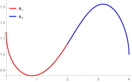
Figure 1: The figure of $a_{\pm}\left(r\right)$.

To examine the presence of a physical singularity, we evaluate the Kretschmann scalar:

$$R_{\mu\nu\rho\sigma}R^{\mu\nu\rho\sigma}=\frac{1}{2}R_{\mu\nu}R^{\mu\nu}=R^{2}$$

$$=\lambda^{4}\left(2r\left(M-r\right)\left(\dot{H}+H^{2}\right)+\left(M-2r\right)H\right)^{2}$$

$$=\frac{\lambda^{4}M^{2}\left(1-\alpha^{\prime}\lambda^{2}\right)^{2}}{A\left(r\right)^{6}}\left(-16C\left(r\right)A\left(r\right)^{3/2}-4M\left(\alpha^{\prime}\lambda^{2}-1\right)B\left(r\right)^{2}+24\left(\alpha^{\prime}\lambda^{2}-1\right)C\left(r\right)B\left(r\right)A\left(r\right)^{1/2}\right)^{2},$$

where

$$A\left(r\right) = \alpha^{\prime}\lambda^{2}\left(M^{2}-8Mr+8r^{2}\right)+8r\left(M-r\right),$$

$$B\left(r\right) = \alpha^{\prime}\lambda^{2}M^{2}-8Mr+8r^{2},$$

$$C\left(r\right) = \sqrt{2}\left(M-2r\right)\sqrt{r\left(M-r\right)}.$$ (3.30)

Therefore, the solutions (3.26) are regular only when $A\left(r\right)=0$ has no any real root. This condition leads to the following result:

$$1\leq\alpha^{\prime}\lambda^{2}<2,$$ (3.31)

which is consistent with the result $\lambda^{2}\sim\frac{1}{\alpha^{\prime}}$ (cosmological constant problem in string theory) within the framework of string theory. The Kretschmann scalar is displayed in Figure (2).

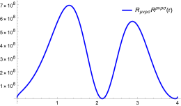
Figure 2: The figure of Kretschmann scalar $0\leq r\leq M$, where we set $\alpha^{\prime}\lambda^{2}=\frac{4}{3}$, $\lambda=100$ and $M=4$.

In summary, the key results of this subsection are as follows:

• The $\alpha^{\prime}$ corrections eliminate the curvature singularity located at $r=0$.

• The $\alpha^{\prime}$ corrections do not affect the event horizon, as it is maintained by $n\left(r\right)=\left(\frac{M}{r}-1\right)^{-1/2}\frac{1}{\lambda r}$ .

4 Two-dimensional regular string black hole in unitary gauge

In this section, we examine the regular black hole solution within the ansatz (2.4) and (2.7). These two ansatz cover the inside and outside regions of the event horizon of two-dimensional black hole separately.

4.1 Inside the event horizon

The solutions inside the event horizon were previously derived in ref. [16], and we provide the main results here. Recalling the two-dimensional black hole metric inside the event horizon:

$$ds^{2} = -dx^{2}+\tan^{2}\left(\frac{\lambda}{2}x\right)dt^{2},$$

$$\Phi = -\ln\left(\sin\left(\lambda x\right)\right),$$ (4.32)

we can extract the ansatz:

$$ds^{2}=-dx^{2}+a_{in}\left(x\right)^{2}dt^{2}.$$ (4.33)

In this background, the EOM of Hohm-Zwiebach action are given by:

$$\ddot{\Phi}_{in}+\frac{1}{2}H_{in}f\left(H_{in}\right) = 0,$$

$$\frac{d}{dx}\left(e^{-\Phi_{in}}f\left(H_{in}\right)\right) = 0,$$

$$\dot{\Phi}_{in}^{2}+g\left(H_{in}\right)+\lambda^{2} = 0,$$ (4.34)

where

$$f\left(H_{in}\right) = \sum_{k=1}^{\infty}\left(-\alpha^{\prime}\right)^{k-1}2^{2\left(k+1\right)}kc_{k}H_{in}^{2k-1}=-2H_{in}-\alpha^{\prime}2H_{in}^{3}+\cdots,$$

$$g\left(H_{in}\right) = \sum_{k=1}^{\infty}\left(-\alpha^{\prime}\right)^{k-1}2^{2k+1}\left(2k-1\right)c_{k}H_{in}^{2k}=-H_{in}^{2}-\alpha^{\prime}\frac{3}{2}H_{in}^{4}+\cdots,$$ (4.35)

and there is an additional constraint: $\dot{g}\left(H_{in}\right)=H_{in}\dot{f}\left(H_{in}\right)$. Since the ansatz is analogous to the cosmological background, we denote $\dot{f}\left(x\right)\equiv\partial_{x}f\left(x\right)$, $H_{in}\left(x\right)\equiv\frac{\dot{a}_{in}\left(x\right)}{a_{in}\left(x\right)}$, $c_{1}=-\frac{1}{8}$, $c_{2}=\frac{1}{64}$, $c_{3}=-\frac{1}{3.2^{7}}$, $c_{4}=\frac{1}{2^{15}}-\frac{1}{2^{12}}\zeta\left(3\right)$ and $c_{k>4}$’s are unknown coefficients for the bosonic case [22]. The regular solutions are given by:

$$\Phi_{in}\left(x\right) = \log\sqrt{\frac{1+\alpha^{\prime}\lambda^{2}}{\sin^{2}\left(\lambda x\right)+\frac{1}{2}\alpha^{\prime}\lambda^{2}\sin^{2}\left(\lambda x\right)\left(\cot^{2}\left(\lambda x\right)+1\right)}},$$

$$H_{in}\left(x\right) = -\frac{\sqrt{2}\lambda\left(\left(\alpha^{\prime}\lambda^{2}+1\right)\cos\left(2\lambda x\right)-1\right)}{\left(\alpha^{\prime}\lambda^{2}+1\right)^{1/2}\left(\alpha^{\prime}\lambda^{2}+1-\cos\left(2\lambda x\right)\right)^{3/2}},$$

$$f_{in}\left(x\right) = -2\sqrt{2}\lambda\left(\frac{\alpha^{\prime}\lambda^{2}+1}{\alpha^{\prime}\lambda^{2}+1-\cos\left(2\lambda x\right)}\right)^{1/2},$$

$$g_{in}\left(x\right) = \frac{\lambda^{2}}{\left(\alpha^{\prime}\lambda^{2}+1-\cos\left(2\lambda x\right)\right)^{2}}\left(-\alpha^{\prime}\lambda^{2}\left(\alpha^{\prime}\lambda^{2}+2\right)+2\left(\alpha^{\prime}\lambda^{2}+1\right)\cos\left(2\lambda x\right)-2\right),$$ (4.36)

and the corresponding scale factor is given by:

$$ds^{2}=a_{in}\left(x\right)^{2}dt^{2}-dx^{2}.$$ (4.37)

with

$$a_{in}\left(x\right) = C_{in}\exp\sqrt{2}\left[\sqrt{\frac{\alpha^{\prime}\lambda^{2}+1}{\alpha^{\prime}\lambda^{2}}}\mathbb{F}\left(x\lambda\left|-\frac{2}{\alpha^{\prime}\lambda^{2}}\right.\right)\right.$$ (4.38)

$$\left.-\sqrt{\frac{\alpha^{\prime}\lambda^{2}}{\alpha^{\prime}\lambda^{2}+1}}\mathbb{E}\left(x\lambda\left|-\frac{2}{\alpha^{\prime}\lambda^{2}}\right.\right)-\frac{\sin\left(2\lambda x\right)}{\sqrt{\left(\alpha^{\prime}\lambda^{2}+1\right)\left(\alpha^{\prime}\lambda^{2}+1-\cos\left(2\lambda x\right)\right)}}\right],$$

where $\mathbb{F}\left(\phi|m\right)$ and $\mathbb{E}\left(\phi|m\right)$ are elliptic integrals of the first and second kinds, and $C_{in}$ is an integral constant. This regular solution has been studied in ref. [16].

Finally, we wish to verify that by using the appropriate coordinate transformation (2.6) on (4.36), we can obtain the expected solution (3.26)

$$H\left(r\right) = \frac{\frac{dx}{dr}\frac{d}{dx}a_{in}\left(x\right)}{a_{in}\left(x\right)}=\frac{dx}{dr}H\left(x\right)$$ (4.39)

$$= -\frac{1}{\lambda M\sqrt{\frac{r}{M}-\frac{r^{2}}{M^{2}}}}\frac{\sqrt{2}\lambda\left(\alpha^{\prime}\lambda^{2}-1\right)\left(\alpha^{\prime}\lambda^{2}-1+\cos\left(2\lambda x\right)\right)}{\left(\left(\alpha^{\prime}\lambda^{2}-1\right)\cos\left(2\lambda x\right)+1\right)^{3/2}}.$$

Then, using the coordinate transformation (2.6): $r/M=\cos^{2}\left(\lambda x/2\right)$, we have

$$H\left(r\right)=-\frac{\sqrt{2}M\left(\alpha\lambda^{2}-1\right)\left(\alpha\lambda^{2}M^{2}-8Mr+8r^{2}\right)}{\sqrt{r(M-r)}\left(\alpha\lambda^{2}\left(M^{2}-8Mr+8r^{2}\right)+8r(M-r)\right)^{3/2}},$$ (4.40)

which agrees with the solution (3.26).

In summary, the following results are obtained in this subsection:

• The curvature singularity located at $x=\pi/\lambda$ can be removed by the $\alpha^{\prime}$ corrections.

• The solution in unitary gauge (4.36) agrees with the solution in Schwarzschild gauge (3.26) using the appropriate coordinate transformation (2.6).

4.2 Outside the event horizon

Firstly, let us consider the metric that describes the region outside the event horizon:

$$ds^{2} = -\tanh^{2}\left(\frac{\lambda}{2}x\right)dt^{2}+dx^{2},$$

$$\Phi = -\ln\left(\sinh\left(\lambda x\right)\right).$$ (4.41)

To apply the Hohm-Zwiebach action, we extract the ansatz from the above metric, which is given by:

$$ds^{2}=dx^{2}-a_{out}\left(x\right)^{2}dt^{2}.$$ (4.42)

This ansatz can be seen as the double wick rotation of the cosmological background, and we use “bar” to denote this situation in the following calculations. The corresponding Hohm-Zwiebach action can be expressed as:

$$\bar{I}_{HZ} = \int d^{3}x\sqrt{-g}e^{-2\phi}\left(R+4\left(\partial\phi\right)^{2}+\frac{1}{4}\alpha^{\prime}\left(R^{\mu\nu\rho\sigma}R_{\mu\nu\rho\sigma}+\ldots\right)+\alpha^{\prime 2}\left(\ldots\right)+\ldots\right)$$ (4.43)

$$= -\int dxe^{-\Phi}\left(-\Phi^{\prime 2}-\sum_{\text{k=1}}^{\infty}\left(-\alpha^{\prime}\right)^{k-1}2^{2k+1}\bar{c}_{k}H_{out}^{2k}\right),$$

where $H_{out}\left(x\right)=\frac{\partial_{x}a_{out}\left(x\right)}{a_{out}\left(x\right)}$ and $A^{\prime}\left(x\right)\equiv\partial_{x}A\left(x\right)$. It is important to note the difference in sign between the actions in (3.10) and (4.43) for the two different ansatz. Moreover, we have $\bar{c}_{1}=c_{1}=-\frac{1}{8}$, $\bar{c}_{2}=-c_{2}=-\frac{1}{64}$, $\bar{c}_{2k-1}=c_{2k-1}$, $\bar{c}_{2k}=-c_{2k}$. Including the cosmological constant term:

$$\bar{I}_{m}=\int d^{3}xe^{-\Phi}\lambda^{2},$$ (4.44)

the corresponding EOM for the action can be expressed as:

$$\Phi^{\prime\prime}+\frac{1}{2}H_{out}f\left(H_{out}\right) = 0,$$

$$\frac{d}{dx}\left(e^{-\Phi_{out}}f\left(H_{out}\right)\right) = 0,$$

$$\Phi_{out}^{\prime 2}+g\left(H_{out}\right)-\lambda^{2} = 0,$$ (4.45)

where there is a constraint $g^{\prime}\left(H_{out}\right)=H_{out}f^{\prime}\left(H_{out}\right)$ and

$$f\left(H_{out}\right) = \sum_{\text{k=1}}^{\infty}\left(-\alpha^{\prime}\right)^{k-1}2^{2\left(k+1\right)}k\bar{c}_{k}H_{out}^{2k-1}=-2H_{out}+\alpha^{\prime}2H_{out}^{3}+\cdots,$$

$$g\left(H_{out}\right) = \sum_{\text{k=1}}^{\infty}\left(-\alpha^{\prime}\right)^{k-1}2^{2k+1}\left(2k-1\right)\bar{c}_{k}H_{out}^{2k}=-H_{out}^{2}+\alpha^{\prime}\frac{3}{2}H_{out}^{4}+\cdots.$$ (4.46)

To calculate the perturbative solutions, we also introduce the variable $\Omega_{out}\equiv e^{-\Phi_{out}}$, $\Omega_{out}^{\prime}=-\Phi_{out}^{\prime}\Omega_{out}$ and $\Omega_{out}^{\prime\prime}=\left(-\Phi_{out}^{\prime\prime}+\Phi_{out}^{\prime 2}\right)\Omega_{out}$. The EOM (4.45) can be written as follows:

$$\Omega_{out}^{\prime\prime}-\left(h\left(H_{out}\right)+\lambda^{2}\right)\Omega_{out} = 0,$$

$$\frac{d}{dx}\left(\Omega_{out}f\left(H_{out}\right)\right) = 0,$$

$$\Omega_{out}^{\prime 2}+\left(g\left(H_{out}\right)-\lambda^{2}\right)\Omega_{out}^{2} = 0,$$ (4.47)

where we define a new function

$$h\left(H_{out}\right)\equiv\frac{1}{2}H_{out}f\left(H_{out}\right)-g\left(H_{out}\right)=-\alpha^{\prime}\frac{1}{2}H_{out}^{4}+\ldots,$$ (4.48)

It is easy to see that $\bar{h}\left(\bar{H}\right)=0$ at the zeroth order of $\alpha^{\prime}$. We assume the perturbative solutions of the EOM (4.47) take the following forms:

$$\Omega_{out}\left(x\right) = \Omega_{0}\left(x\right)+\alpha^{\prime}\Omega_{1}\left(x\right)+\alpha^{\prime 2}\Omega_{2}\left(x\right)+\ldots,$$

$$H_{out}\left(x\right) = H_{0}\left(x\right)+\alpha^{\prime}H_{1}\left(x\right)+\alpha^{\prime 2}H_{2}\left(x\right)+\ldots.$$ (4.49)

where $\Omega_{i}$ and $\bar{H}_{i}$ represent the $i$-th order of the perturbative solutions. Using these perturbative forms, the functions $h\left(H_{out}\right)$, $f\left(H_{out}\right)$ and $g\left(H_{out}\right)$ can be expressed as:

$$h\left(H_{out}\right) = -\alpha^{\prime}\frac{1}{2}H_{0}^{4}+\ldots,$$

$$f\left(H_{out}\right) = -2H_{0}+\alpha^{\prime}\left(2H_{0}^{3}-2H_{1}\right)+\cdots,$$

$$g\left(H_{out}\right) = -H_{0}^{2}+\alpha^{\prime}\left(\frac{3}{2}H_{0}^{4}-2H_{0}H_{1}\right)+\cdots.$$ (4.50)

By substituting these perturbative forms back into the EOM (4.47)and solving the resulting differential equations at each order of $\alpha^{\prime}$, we obtain $\Omega_{i}$ and $\bar{H}_{i}$. At the zeroth order of $\alpha^{\prime}$ , the EOM (4.47) gives the expected solution:

$$\Omega_{0}^{\prime\prime}-\lambda^{2}\Omega_{0} = 0,$$

$$\frac{d}{dx}\left(-2\Omega_{0}\bar{H}_{0}\right) = 0,$$

$$\Omega_{0}^{\prime 2}-\left(H_{0}^{2}+\lambda^{2}\right)\Omega_{0}^{2} = 0,$$ (4.51)

As expected, the zeroth order solution is given by:

$$\Omega_{0} = \sinh\left(\lambda x\right),$$

$$H_{0} = \lambda\text{csch}\left(\lambda x\right),$$ (4.52)

which corresponds to the solution (2.4). Moving on to the first order of $\alpha^{\prime}$, the EOM (4.47) yield:

$$\alpha^{\prime}\Omega_{1}^{\prime\prime}+\alpha^{\prime}\left(\frac{1}{2}H_{0}^{4}\Omega_{0}-\lambda^{2}\Omega_{1}\right) = 0,$$

$$\alpha^{\prime}\left(-2H_{0}\Omega_{1}+\left(2H_{0}^{3}-2H_{1}\right)\Omega_{0}\right) = 0,$$

$$2\alpha^{\prime}\Omega_{0}^{\prime}\Omega_{1}^{\prime}-2\alpha^{\prime}\left(H_{0}^{2}+\lambda^{2}\right)\Omega_{0}\Omega_{1}+\alpha^{\prime}\left(\frac{3}{2}H_{0}^{4}-2H_{0}H_{1}\right)\Omega_{0}^{2} = 0.$$ (4.53)

The solution is given by:

$$\Omega_{1}\left(x\right) = -\frac{\lambda^{2}}{4}\mathrm{csch}\left(\lambda x\right),$$

$$H_{1}\left(x\right) = \frac{\lambda^{3}}{4}\left(4+\cosh\left(2\lambda x\right)\right)\mathrm{csch}^{3}\left(\lambda x\right).$$ (4.54)

Therefore, the perturbative solution up to the first two orders of $\alpha^{\prime}$ is given by:

$$H_{out}\left(x\right) = \lambda\text{csch}\left(\lambda x\right)+\frac{\lambda^{3}}{4}\left(4+\cosh\left(2\lambda x\right)\right)\mathrm{csch}^{3}\left(\lambda x\right)\alpha^{\prime}+\cdots,$$

$$\Omega_{out}\left(x\right) = \sinh\left(\lambda x\right)-\frac{\lambda^{2}}{4}\mathrm{csch}\left(\lambda x\right)\alpha^{\prime}+\cdots,$$ (4.55)

Using the notation in (3.15), we can express $\Phi_{out}\left(x\right)$ as

$$\Phi_{out}\left(x\right)=-\log\left(\sinh\left(\lambda x\right)\right)+\frac{\lambda^{2}}{4}\mathrm{csch}^{2}\left(\lambda x\right)\alpha^{\prime}+\cdots.$$ (4.56)

Based on the perturbative solutions (4.55) and (4.56), and after numerous trial and error attempts, we can determine a non-perturbative and non-singular solution:

$$\Phi_{out}\left(x\right) = -\frac{1}{2}\log\left[\frac{2\sinh^{2}\left(\lambda x\right)}{\alpha^{\prime}\lambda^{2}\left(\coth^{2}\left(\lambda x\right)-1\right)+2}\right],$$

$$H_{out}\left(x\right) = \frac{\sqrt{2}\lambda\left(\alpha^{\prime}\lambda^{2}\left(4\alpha^{\prime}\lambda^{2}-7\right)+\left(6\alpha^{\prime}\lambda^{2}-4\right)\cosh\left(2\lambda x\right)+\left(\alpha^{\prime}\lambda^{2}+1\right)\cosh\left(4\lambda x\right)+3\right)}{\left(\alpha^{\prime}\lambda^{2}+2\right)\left(\alpha^{\prime}\lambda^{2}+\cosh\left(2\lambda x\right)-1\right)^{5/2}},$$

$$f_{out}\left(x\right) = -\frac{\lambda\left(\alpha^{\prime}\lambda^{2}+2\right)\text{csch}^{2}\left(\lambda x\right)\sqrt{\alpha^{\prime}\lambda^{2}+\cosh\left(2\lambda x\right)-1}}{\sqrt{2}},$$

$$g_{out}\left(x\right) = -\frac{\lambda^{2}\left(3\alpha^{\prime}\lambda^{2}\left(\alpha^{\prime}\lambda^{2}+2\right)+4\alpha^{\prime 2}\lambda^{4}\text{csch}^{2}\left(\lambda x\right)+2\left(\alpha^{\prime}\lambda^{2}+1\right)\cosh\left(2\lambda x\right)-2\right)}{\left(\alpha^{\prime}\lambda^{2}+\cosh\left(2\lambda x\right)-1\right)^{2}}.$$ (4.57)

From this solution, we can obtain the scale factor:

$$ds^{2}=-a_{out}\left(x\right)^{2}dt^{2}+dx^{2}.$$ (4.58)

with

$$a_{out}\left(x\right) = C_{out}\exp 2\sqrt{2}\left[\frac{-2\alpha^{\prime}\lambda^{2}-3}{3\sqrt{\alpha^{\prime}}\lambda\left(\alpha^{\prime}\lambda^{2}+2\right)}i\mathbb{F}\left(ix\lambda\left|\frac{2}{\alpha^{\prime}\lambda^{2}}\right.\right)+\frac{\sqrt{\alpha^{\prime}}\lambda\left(2\alpha^{\prime}\lambda^{2}-5\right)}{3\left(\alpha^{\prime 2}\lambda^{4}-4\right)}i\mathbb{E}\left(ix\lambda\left|\frac{2}{\alpha^{\prime}\lambda^{2}}\right.\right)+\right.$$ (4.59)

$$\left.\frac{\sinh\left(2\lambda x\right)\left(\alpha^{\prime}\lambda^{2}\left(\alpha^{\prime}\lambda^{2}-5\right)+\left(2\alpha^{\prime}\lambda^{2}-5\right)\cosh\left(2\lambda x\right)+5\right)}{3\left(\alpha^{\prime 2}\lambda^{4}-4\right)\left(\alpha^{\prime}\lambda^{2}+\cosh\left(2\lambda x\right)-1\right)^{3/2}}\right],$$

where $\mathbb{F}\left(\phi|m\right)$ and $\mathbb{E}\left(\phi|m\right)$ are elliptic integrals of the first and second kinds, and $C_{out}$ is an integral constant. The corresponding Kretschmann scalar is given by:

$$R_{\mu\nu\rho\sigma}R^{\mu\nu\rho\sigma}=\frac{1}{2}R_{\mu\nu}R^{\mu\nu}=R^{2}=4\left(\frac{\ddot{a}}{a}\right)^{2}$$

$$= \frac{16\lambda^{2}}{\left(\alpha\lambda^{2}+2\right)^{2}\left(\alpha\lambda^{2}+\cosh\left(2\lambda x\right)-1\right)^{5}}\left[8\alpha^{\prime 4}\lambda^{8}+16\alpha^{\prime 3}\lambda^{6}\sinh^{2}\left(\lambda x\right)\left(\cosh(2\lambda x)+4\right)\right.$$

$$+4\alpha^{\prime 2}\lambda^{4}\sinh^{4}\left(\lambda x\right)\left(16\cosh\left(2\lambda x\right)+\cosh\left(4\lambda x\right)+41\right)-\sqrt{2}\left(\alpha^{\prime}\lambda^{2}+2\right)\sinh^{3}\left(\lambda x\right)\cosh\left(\lambda x\right)\times$$

$$\sqrt{\alpha^{\prime}\lambda^{2}+\cosh\left(2\lambda x\right)-1}\left(\alpha^{\prime}\lambda^{2}\left(4\alpha^{\prime}\lambda^{2}\left(7-2\alpha^{\prime}\lambda^{2}\right)-21\right)\right.$$

$$\left.+\left(-6\alpha^{\prime 2}\lambda^{4}+20\alpha^{\prime}\lambda^{2}-4\right)\cosh\left(2\lambda x\right)+\left(\alpha^{\prime}\lambda^{2}+1\right)\cosh\left(4\lambda x\right)+3\right)$$

$$\left.+32\alpha^{\prime}\lambda^{2}\sinh^{6}\left(\lambda x\right)(\cosh\left(2\lambda x\right)+4)+32\sinh^{8}\left(\lambda x\right)\right].$$

The Kretschmann scalar is displayed in Figure (3). It is demonstrates that the solution outside the event horizon ($x\geq 0$) remains regular and approaches an asymptotically flat behavior as $x\rightarrow\infty$.

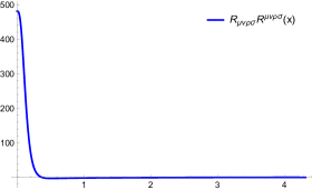
Figure 3: The figure of Kretschmann scalar, where $\lambda=1$ and $\alpha^{\prime}=\frac{1}{16}$.

Finally, we wish establish a junction between the outside solution (4.58) and the inside solution (4.37) at the event horizon. Achieving this connection implies that the event horizon remains unaffected by the $\alpha^{\prime}$ corrections. Specifically, since the event horizon is located at $x=0$ in both solutions, we require $a_{in}\left(0\right)=a_{out}\left(0\right)$, leading to the following constraint:

$$C_{in}=C_{out}.$$ (4.61)

In summary, we have the following results in this subsection:

• The event horizon is not affected by the $\alpha^{\prime}$ corrections. This result is consistent with the findings in the Schwarzschild gauge.

• The $\alpha^{\prime}$ corrections do not introduce additional singularities outside the event horizon.

• The singularity of the dilaton in the perturbative solution is not removed by the $\alpha^{\prime}$ corrections.

5 Conclusion

In this paper, we calculated the non-perturbative and non-singular string black hole solutions in both the Schwarzschild gauge and unitary gauge. The results obtained from these two gauges were in agreement, and they can be transformed into each other through appropriate coordinate transformations. Our findings highlight that the $\alpha^{\prime}$ corrections in string theory are capable of eliminating the curvature singularities of two-dimensional black holes. Furthermore, in the perturbative limit $\alpha^{\prime}\rightarrow 0$, our solution matches the divergent solutions derived from the tree-level string effective action. The implications of our research are as follows:

• The curvature singularity of the two-dimensional black hole can be removed.

• The event horizon remains unaffected by the $\alpha^{\prime}$ corrections.

• The $\alpha^{\prime}$ corrections do not introduce any additional singularities to the two-dimensional black hole.

In the following works, it is worthwhile to explore the following issues:

• How to remove the curvature singularities of more general black holes is a significant problem, such as spherically symmetric black holes. This black hole solutions are more relevant to our physical world. However, the metric of a spherically symmetric black hole depends on two coordinates $r$ and $\theta$, which breaks the $O\left(d,d\right)$ symmetry. The Hohm-Zwiebach action cannot be applied directly.

• Investigating higher-dimensional black holes is of great interest. Given that the line element of a higher-dimensional black hole is anisotropic, the Hohm-Zwiebach action needs to incorporate the multi-trace term, which adds complexity to the calculations. Hence, developing a method to compute perturbative and non-perturbative solutions while accounting for the multi-trace terms is necessary.

• Exploring the incorporation of the Kalb-Ramond field [23] is also an interested direction. For instance, the BTZ black hole solution in string theory requires a non-vanishing Kalb-Ramond field. This implies that if we aim to eliminate the curvature singularity in this black hole, the Hohm-Zwiebach action must include the Kalb-Ramond field as well.

Acknowledgements We are deeply indebted to Xin Li, Peng Wang, Houwen Wu and Haitang Yang for many illuminating discussions and suggestions. This work is supported in part by NSFC (Grant No. 12105031), and the Postdoctoral Science Foundation of Chongqing (Grant No. cstc2021jcyj-bshX0227).

References

- [1] R. Penrose, “Gravitational collapse and space-time singularities,” Phys. Rev. Lett. 14, 57-59 (1965) doi:10.1103/PhysRevLett.14.57
- [2] S. Hawking, “Occurrence of singularities in open universes,” Phys. Rev. Lett. 15, 689-690 (1965) doi:10.1103/PhysRevLett.15.689
- [3] O. Hohm and B. Zwiebach, “T-duality Constraints on Higher Derivatives Revisited,” JHEP 1604, 101 (2016) doi:10.1007/JHEP04(2016)101 [arXiv:1510.00005 [hep-th]].
- [4] O. Hohm and B. Zwiebach, “Non-perturbative de Sitter vacua via corrections,” Int. J. Mod. Phys. D 28, no.14, 1943002 (2019) doi:10.1142/S0218271819430028 [arXiv:1905.06583 [hep-th]].
- [5] O. Hohm and B. Zwiebach, “Duality invariant cosmology to all orders in ’,” Phys. Rev. D 100, no.12, 126011 (2019) doi:10.1103/PhysRevD.100.126011 [arXiv:1905.06963 [hep-th]].
- [6] A. Sen, “O(d) x O(d) symmetry of the space of cosmological solutions in string theory, scale factor duality and two-dimensional black holes,” Phys. Lett. B 271, 295 (1991). doi:10.1016/0370-2693(91)90090-D
- [7] A. Sen, “Twisted black p-brane solutions in string theory,” Phys. Lett. B 274, 34 (1992) doi:10.1016/0370-2693(92)90300-S [hep-th/9108011].
- [8] G. Veneziano, “Scale factor duality for classical and quantum strings,” Phys. Lett. B 265, 287 (1991). doi:10.1016/0370-2693(91)90055-U
- [9] K. A. Meissner and G. Veneziano, “Symmetries of cosmological superstring vacua,” Phys. Lett. B 267, 33 (1991). doi:10.1016/0370-2693(91)90520-Z
- [10] K. A. Meissner, “Symmetries of higher order string gravity actions,” Phys. Lett. B 392, 298 (1997) doi:10.1016/S0370-2693(96)01556-0 [hep-th/9610131].
- [11] P. Wang, H. Wu, H. Yang and S. Ying, “Non-singular string cosmology via corrections,” JHEP 1910, 263 (2019) doi:10.1007/JHEP10(2019)263 [arXiv:1909.00830 [hep-th]].
- [12] P. Wang, H. Wu, H. Yang and S. Ying, “Construct corrected or loop corrected solutions without curvature singularities,” JHEP 01, 164 (2020) doi:10.1007/JHEP01(2020)164 [arXiv:1910.05808 [hep-th]].
- [13] P. Wang, H. Wu and H. Yang, “Are nonperturbative AdS vacua possible in bosonic string theory?,” Phys. Rev. D 100, no. 4, 046016 (2019) doi:10.1103/PhysRevD.100.046016 [arXiv:1906.09650 [hep-th]].
- [14] M. Gasperini and G. Veneziano, “Non-singular pre-big bang scenarios from all-order corrections,” [arXiv:2305.00222 [hep-th]].
- [15] L. Song and D. Chen, “Two non-perturbative corrected or loop corrected string cosmological solutions,” [arXiv:2306.07031 [hep-th]].
- [16] S. Ying, “Two-dimensional regular string black hole via complete corrections,” [arXiv:2212.03808 [hep-th]]. accepted by Eur.Phys.J.C
- [17] S. Ying, “Three dimensional regular black string via loop corrections,” JHEP 03, 044 (2023) doi:10.1007/JHEP03(2023)044 [arXiv:2212.14785 [hep-th]].
- [18] T. Codina, O. Hohm and B. Zwiebach, “2D Black Holes, Bianchi I Cosmologies, and ,” [arXiv:2304.06763 [hep-th]].
- [19] G. Mandal, A. M. Sengupta and S. R. Wadia, “Classical solutions of two-dimensional string theory,” Mod. Phys. Lett. A 6, 1685-1692 (1991) doi:10.1142/S0217732391001822
- [20] J. H. Horne and G. T. Horowitz, “Exact black string solutions in three-dimensions,” Nucl. Phys. B 368, 444-462 (1992) doi:10.1016/0550-3213(92)90536-K [arXiv:hep-th/9108001 [hep-th]].
- [21] E. Witten, “String theory and black holes,” Phys. Rev. D 44, 314 (1991) doi:10.1103/PhysRevD.44.314
- [22] T. Codina, O. Hohm and D. Marques, “General string cosmologies at order ’3,” Phys. Rev. D 104, no.10, 106007 (2021) doi:10.1103/PhysRevD.104.106007 [arXiv:2107.00053 [hep-th]].
- [23] H. Bernardo, P. R. Chouha and G. Franzmann, “Kalb-Ramond backgrounds in ’-complete cosmology,” JHEP 09, 109 (2021) doi:10.1007/JHEP09(2021)109 [arXiv:2104.15131 [hep-th]].