Evolution of local relaxed states and the modelling of viscoelastic fluids

Abstract

We introduce a class of continuum mechanical models aimed at describing the behavior of viscoelastic fluids by incorporating concepts originated in the theory of solid plasticity. Within this class, even a simple model with constant material parameters is able to qualitatively reproduce a number of experimental observations in both simple shear and extensional flows, including linear viscoelastic properties, the rate dependence of steady-state material functions, the stress overshoot in incipient shear flows, and the difference in shear and extensional rheological curves. Furthermore, by allowing the relaxation time of the model to depend on the total strain, we can reproduce some experimental observations of the non-attainability of steady flows in uniaxial extension, and link this to a concept of polymeric jamming or effective solidification. Remarkably, this modelling framework helps in understanding the interplay between different mechanisms that may compete in determining the rheology of non-Newtonian materials.

Keywords: viscoelasticity, non-Newtonian rheology, tensorial model, logarithmic stress

MSC Classification (2020): 76A10 - 74D99

1 Introduction

Rheology deals with the way materials deform when forces are applied to them. The subject of its studies comprises both fluid-like and solid-like behaviors, that can appear in combination when dealing with complex fluids. At opposite ends of the viscoelastic spectrum we find Newtonian viscous fluids and elastic solids. The former resist shear by dissipating energy and can strain indefinitely under an applied stress, the latter can store energy and balance the applied stress to reach a static configuration, always remembering their original shape. To be able to describe intermediate material responses, we need to address the evolution of the elastically relaxed shape, as well as that of the actual deformation.

Viscoelastic models in continuum mechanics go all the way back to Maxwell and reached a fundamental turning point in their systematic treatment with the work of Oldroyd [1, 2]. In the approach of differential models, the flow equations are typically coupled to an evolution equation for either the elastic stress itself or a conformation tensor. The time-dependence of the elastically relaxed shape is implicit in these relations. Among the several important contributions that are by now textbook material [3, 4], we would like to highlight the models by Giesekus [5, 6] and by Phan-Thien & Tanner [7] for their tensorial structure and usefulness in fitting experimental data. A very informative review of Oldroyd’s influence on complex fluids modelling can be found in a recent article by Beris [8].

In this work, we wish to approach the modelling of viscoelastic materials in a somewhat different way, by combining concepts coming from the theory of solid plasticity with a fluid mechanics framework. Our goal is to capture the qualitative behavior of viscoelastic fluids measured in experiments with constitutive models in which the material parameters have a clear mechanical meaning. We present a tensorial model that displays the same linear viscoelastic properties of the upper-convected Maxwell model, but it is able, with the same number of material parameters, to capture rate-dependent effects in transient shear flows.

The main point of our approach is that we obtain the evolution of the elastic stress as a result of the evolution of the current deformation gradient and of a tensorial description of the local relaxed state. The evolution of the former quantity is fully determined by the continuum kinematics, while the structure of the equation for the relaxed state is similar to the flow rules that are postulated in plasticity theory. Within our framework, viscoelastic fluids emerge as an interpolation between purely viscous fluids and solids, controlled precisely by the characteristic time of the plastic evolution. This is a feature not always present in viscoelastic models, as pointed out by Snoeijer et al. [9] in a recent review. A second important aspect is the use of logarithimic relations between the elastic stress and the strain measure, akin to the Hencky strain approach. In fact, the matrix logarithm allows to link the strains, that naturally belong to a multiplicative group of linear transformations, to stresses, that are additive elements of a linear space of tensors. We first propose a basic model in which material parameters are assumed constant. This can of course be relaxed to better represent real fluids. Nevertheless, we can already capture nontrivial qualitative features of viscoelastic flows. We are able to obtain a dependence of rheological curves on the shear rate and even on the flow type without any such dependence in the material parameters. Indeed, those effects turn out to be a result of how the different flows affect the elastic part of the stress, with particular reference to the dynamics of the principal stress directions.

The paper is organized as follows. In Section 2, we introduce the basic evolution equations and a new class of viscoelastic constitutive models. Section 3 is devoted to finding the evolution equation for the elastic strain (akin to a conformation tensor) implied by our model and to the analysis of the energy balance, that highlights the presence of two distinct dissipative effects. Focusing on the special case of a model with constant coefficients, we present in Section 4 analytical results about small-amplitude oscillatory flows, while stress growth and stress relaxation predictions are reported in Section 5 and 6, respectively. To give a first example of the flexibility of our approach, we introduce, in Section 7, a model that captures a strain-induced fluid-solid transition sometimes observed in transient uniaxial extension measurements. Dimensionless numbers that can be associated with the proposed model are discussed in Section 8. In the final Section 9, we conclude by summarizing our main results and addressing further research directions.

We aimed at giving a concise presentation of a general modelling strategy for viscoelastic materials and of a few paradigmatic examples of its effectiveness in reproducing the qualitative features of experimental measurements. We kept technicalities to a minimum while presenting rigorous computations to help the reader grasp the key features of our approach. Several extensions of this work can be foreseen, especially in the direction of including multiple relaxation times and finite extensibility effects. What we wish to stress once more is the importance of taking into account an evolution equation for tensorial descriptors of the local elastically-relaxed state as a central part of constitutive models.

2 Flow equations, kinematics, and constitutive relations

In this section, we introduce the basic evolution equations for a general continuum in the Eulerian setting. We denote by $\rho$ the mass density, that we assume constant and uniform, and by $\bm{u}(\bm{x},t)$ the velocity field at point $\bm{x}$ and time $t$. To be able to follow the material deformation, we introduce the placement ${\bm{\varphi}}(\bm{X},t)$ that gives the position at time $t$ of a material point labelled with $\bm{X}$ and solves the nonlinear equation $\partial_{t}{\bm{\varphi}}(\bm{X},t)=\bm{u}({\bm{\varphi}}(\bm{X},t),t)$. We define the Eulerian deformation gradient $\mathsf{F}(\bm{x},t):=\nabla_{\bm{X}}{\bm{\varphi}}|_{\bm{X}=\hat{{\bm{\varphi}}}(\bm{x},t)}$ with $\hat{{\bm{\varphi}}}$ the spatial inverse of ${\bm{\varphi}}$, such that ${\bm{\varphi}}(\hat{{\bm{\varphi}}}(\bm{x},t),t)=\bm{x}$. For the sake of clarity, we use the following notation for the material time derivative:

$$\mathcal{D}_{\bm{u}}:=\frac{\partial}{\partial t}+\bm{u}\cdot\nabla.$$

The balance of linear momentum gives rise to the evolution equation

$$\rho\mathcal{D}_{\bm{u}}\bm{u}=\operatorname{\mathrm{div}}\bm{\sigma}$$ (1)

for the velocity field, driven by the Cauchy stress tensor $\bm{\sigma}$. We neglect external forces for simplicity. Incompressiblity is expressed by the constraint $\operatorname{\mathrm{div}}\bm{u}=0$.

Regarding the evolution equation for the deformation gradient $\mathsf{F}$ in Eulerian coordinates, it reads

$$\mathcal{D}_{\bm{u}}\mathsf{F}=\nabla\bm{u}\mathsf{F}.$$ (2)

Equation (2) is an exact kinematic relation between the velocity and the displacement of fluid elements and does not contain any constitutive assumption. We note that for incompressible deformations $\det\mathsf{F}=1$. This property is preserved by equation (2) thanks to the fact that $\operatorname{\mathrm{tr}}(\nabla\bm{u})=\operatorname{\mathrm{div}}\bm{u}=0$.

A continuum model is specified by prescribing constitutive relations between the Cauchy stress $\bm{\sigma}$ and the kinematic fields that identify the state of the material, such as $\nabla\bm{u}$ and $\mathsf{F}$. Since we consider incompressible models, we introduce the pressure field $p$ and take $\bm{\sigma}=-p{\mathsf{I}}+{\mathsf{T}}$, with a pressure term proportional to the identity matrix ${\mathsf{I}}$ and a treceless extra stress ${\mathsf{T}}$. The latter can be further decomposed as the sum of a viscous contribution ${\mathsf{T}}_{\mathrm{vi}}$ plus an elastic one ${\mathsf{T}}_{\mathrm{el}}$, so that $\bm{\sigma}=-p{\mathsf{I}}+{\mathsf{T}}_{\mathrm{vi}}+{\mathsf{T}}_{\mathrm{el}}$. In what follows, we assume ${\mathsf{T}}_{\mathrm{vi}}=2\eta\mathsf{D}$, wherein a viscosity $\eta\geq 0$ multiplies the symmetric part of the velocity gradient $\mathsf{D}:=(\nabla\bm{u}+\nabla\bm{u}^{\mathsf{T}})/2$. At this stage, we pose no restriction on the possibly nonlinear dependence of $\eta$ on other kinematic descriptors. In later sections we will consider the simplest case of a constant viscosity to highlight the role of the elastic term in determining the model rheology.

To propose a relation for the elastic stress ${\mathsf{T}}_{\mathrm{el}}$ we need to introduce a tensorial description of the local state of deformation in which no elastic response would be present. Recall that the deformation gradient $\mathsf{F}$ is a linear transformation from the space of material vectors to that of spatial vectors. In purely elastic theories, the relaxed state is most often assumed to be realized by a reference material configuration, so that $\mathsf{F}$ maps relaxed (material) line elements into stretched (spatial) line elements. We are interested in a more general situation and then we introduce the tensor field $\mathsf{F}_{\mathrm{R}}$, that maps the reference material line elements into relaxed material line elements. We stress that $\mathsf{F}_{\mathrm{R}}$ need not be the gradient of a global configuration of the continuum. With this, we can define the elastic deformation gradient as $\mathsf{F}_{\mathrm{el}}:=\mathsf{F}\mathsf{F}_{\mathrm{R}}^{-1}$, from which we obtain the right and left Cauchy–Green tensors $\mathsf{C}_{\mathrm{el}}:=\mathsf{F}_{\mathrm{el}}^{\mathsf{T}}\mathsf{F}_{\mathrm{el}}$ and $\mathsf{B}_{\mathrm{el}}:=\mathsf{F}_{\mathrm{el}}\mathsf{F}_{\mathrm{el}}^{\mathsf{T}}$, respectively, sometimes referred to as elastic strain tensors. The former maps relaxed into relaxed line elements, while the latter maps spatial into spatial line elements. As a consequence, both quantities are objective: $\mathsf{B}_{\mathrm{el}}$ is covariant as $\bm{\sigma}$ should be, while $\mathsf{C}_{\mathrm{el}}$ is frame-invariant, as is $\mathsf{F}_{\mathrm{R}}$, given that relaxed line elements are still material ones. By introducing the constant elastic modulus $\kappa\geq 0$, we can then postulate

$${\mathsf{T}}_{\mathrm{el}}=\kappa\log\mathsf{B}_{\mathrm{el}}=\kappa\log(\mathsf{F}\mathsf{F}_{\mathrm{R}}^{-1}\mathsf{F}_{\mathrm{R}}^{-\mathsf{T}}\mathsf{F}^{\mathsf{T}}).$$ (3)

We stress the fact that, by using $\mathsf{B}_{\mathrm{el}}$ in the definition of the stress, we make sure that no elastic response arises when the relative deformation between $\mathsf{F}$ and $\mathsf{F}_{\mathrm{R}}$ is just a rigid rotation. Moreover, the fact that for incompressible motions we have $\det\mathsf{F}=\det\mathsf{F}_{\mathrm{R}}=1$ implies that $\det\mathsf{B}_{\mathrm{el}}=1$ and so $\operatorname{\mathrm{tr}}{\mathsf{T}}_{\mathrm{el}}=\kappa\operatorname{\mathrm{tr}}\log\mathsf{B}_{\mathrm{el}}=0$, as is desirable for a term entering the extra stress.

In viscoelastic materials, the microscopic arrangement of molecules determines the state at which the system would converge in the absence of applied forces. This state can evolve in time as a result of deformations and stresses. We thus need to postulate a suitable evolution equation for $\mathsf{F}_{\mathrm{R}}$. Such an equation should imply that, if we keep the material in a static configuration in which some elastic stress is active, then $\mathsf{F}_{\mathrm{R}}$ converges exponentially to $\mathsf{F}$ with a characteristic time-scale $\tau_{\mathrm{r}}\geq 0$ and the elastic stress relaxes to zero. A possible choice consistent with this picture, preserving the condition $\det\mathsf{F}_{\mathrm{R}}=1$, and involving only frame-invariant quantities is given by

$$\mathcal{D}_{\bm{u}}\mathsf{F}_{\mathrm{R}}=\frac{1}{2\tau_{\mathrm{r}}}\log(\mathsf{C}_{\mathrm{el}})\mathsf{F}_{\mathrm{R}}.$$ (4)

The factor of $2$ in front of $\tau_{\mathrm{r}}$ comes from the fact that $\log\mathsf{C}_{\mathrm{el}}$ contains twice the elastic strain of the material and it is what we need to have the stress relax as $e^{-t/\tau_{\mathrm{r}}}$ in static experiments. As is the case for $\eta$, the relaxation time $\tau_{\mathrm{r}}$ can depend on other quantities that describe the state of the material.

In summary, the evolution equations of the present model are (2), (4), and the linear momentum balance

$$\rho\mathcal{D}_{\bm{u}}\bm{u}=-\nabla p+\operatorname{\mathrm{div}}(2\eta\mathsf{D}+\kappa\log\mathsf{B}_{\mathrm{el}}).$$ (5)

Boundary conditions must be specified only for the velocity field $\bm{u}$, while initial conditions are also needed for $\mathsf{F}$ and $\mathsf{F}_{\mathrm{R}}$.

3 Evolution of the elastic strain and energy balance

The tensorial measure of elastic strain provided by $\mathsf{B}_{\mathrm{el}}$ satisfies an evolution equation that is determined by those of $\mathsf{F}$ and $\mathsf{F}_{\mathrm{R}}$. Remembering equations (2) and (4), we get

$$\mathsf{O}=\mathcal{D}_{\bm{u}}(\mathsf{F}^{-1}\mathsf{F})=(\mathcal{D}_{\bm{u}}\mathsf{F}^{-1})\mathsf{F}+\mathsf{F}^{-1}(\mathcal{D}_{\bm{u}}\mathsf{F}),$$

from which

$$\mathcal{D}_{\bm{u}}\mathsf{F}^{-1}=-\mathsf{F}^{-1}(\mathcal{D}_{\bm{u}}\mathsf{F})\mathsf{F}^{-1}=-\mathsf{F}^{-1}\nabla\bm{u}\qquad\text{and}\qquad\mathcal{D}_{\bm{u}}\mathsf{F}^{-\mathsf{T}}=-\nabla\bm{u}^{\mathsf{T}}\mathsf{F}^{-\mathsf{T}},$$

and

$$\mathsf{O}=\mathcal{D}_{\bm{u}}(\mathsf{F}_{\mathrm{R}}^{-1}\mathsf{F}_{\mathrm{R}})=(\mathcal{D}_{\bm{u}}\mathsf{F}_{\mathrm{R}}^{-1})\mathsf{F}_{\mathrm{R}}+\mathsf{F}_{\mathrm{R}}^{-1}(\mathcal{D}_{\bm{u}}\mathsf{F}_{\mathrm{R}}),$$

from which

$$\mathcal{D}_{\bm{u}}\mathsf{F}_{\mathrm{R}}^{-1}=-\mathsf{F}_{\mathrm{R}}^{-1}(\mathcal{D}_{\bm{u}}\mathsf{F}_{\mathrm{R}})\mathsf{F}_{\mathrm{R}}^{-1}=-\frac{1}{2\tau_{\mathrm{r}}}\mathsf{F}_{\mathrm{R}}^{-1}\log(\mathsf{C}_{\mathrm{el}})\qquad\text{and}\qquad\mathcal{D}_{\bm{u}}\mathsf{F}_{\mathrm{R}}^{-\mathsf{T}}=-\frac{1}{2\tau_{\mathrm{r}}}\log(\mathsf{C}_{\mathrm{el}})\mathsf{F}_{\mathrm{R}}^{-\mathsf{T}}.$$

With these results we can easily compute

$$\mathcal{D}_{\bm{u}}\mathsf{B}_{\mathrm{el}}=\mathcal{D}_{\bm{u}}(\mathsf{F}\mathsf{F}_{\mathrm{R}}^{-1}\mathsf{F}_{\mathrm{R}}^{-\mathsf{T}}\mathsf{F}^{\mathsf{T}})=\nabla\bm{u}\mathsf{B}_{\mathrm{el}}+\mathsf{B}_{\mathrm{el}}\nabla\bm{u}^{\mathsf{T}}-\frac{1}{\tau_{\mathrm{r}}}\mathsf{F}\mathsf{F}_{\mathrm{R}}^{-1}(\log\mathsf{C}_{\mathrm{el}})\mathsf{F}_{\mathrm{R}}^{-\mathsf{T}}\mathsf{F}^{\mathsf{T}}.$$ (6)

By applying the polar decomposition, we define the orthogonal tensor $\mathsf{R}_{\mathrm{el}}$ via the identity $\mathsf{F}\mathsf{F}_{\mathrm{R}}^{-1}=\mathsf{B}_{\mathrm{el}}^{\frac{1}{2}}\mathsf{R}_{\mathrm{el}}$. Moreover, any analytic function $f$ of the tensors $\mathsf{C}_{\mathrm{el}}$ and $\mathsf{B}_{\mathrm{el}}$ is such that $f(\mathsf{B}_{\mathrm{el}})=\mathsf{R}_{\mathrm{el}}f(\mathsf{C}_{\mathrm{el}})\mathsf{R}_{\mathrm{el}}^{-1}$, entailing the identity

$$\mathsf{F}\mathsf{F}_{\mathrm{R}}^{-1}(\log\mathsf{C}_{\mathrm{el}})\mathsf{F}_{\mathrm{R}}^{-\mathsf{T}}\mathsf{F}^{\mathsf{T}}=\mathsf{B}_{\mathrm{el}}^{\frac{1}{2}}(\log\mathsf{B}_{\mathrm{el}})\mathsf{B}_{\mathrm{el}}^{\frac{1}{2}}=\mathsf{B}_{\mathrm{el}}\log\mathsf{B}_{\mathrm{el}}.$$ (7)

Substituting (7) into (6), we finally obtain

$$\mathcal{D}_{\bm{u}}\mathsf{B}_{\mathrm{el}}=\nabla\bm{u}\mathsf{B}_{\mathrm{el}}+\mathsf{B}_{\mathrm{el}}\nabla\bm{u}^{\mathsf{T}}-\frac{1}{\tau_{\mathrm{r}}}\mathsf{B}_{\mathrm{el}}\log\mathsf{B}_{\mathrm{el}}.$$ (8)

We stress that the first two terms on the right-hand side of (8) are of a kinematic nature, since they descend directly from the definition of $\mathsf{B}_{\mathrm{el}}$ and equation (2). Together with the material derivative they constitute a specific objective rate, which is not postulated but is rather a consequence of basic kinematics. The last term depends instead on the constitutive choice we made about the dynamics of $\mathsf{F}_{\mathrm{R}}$, intimately linked to the form of the elastic stress as well. Lastly, if $\det\mathsf{B}_{\mathrm{el}}=1$ at the initial time, then it remains such for all times, because $\operatorname{\mathrm{tr}}(\nabla\bm{u})=0=\operatorname{\mathrm{tr}}(\log\mathsf{B}_{\mathrm{el}})$.

It is finally instructive to compute the energy balance implied by our model. For a smooth divergence-free velocity field $\bm{u}$ that satisfies homogeneous boundary conditions in a domain $\Omega$, we can multiply equation (5) by $\bm{u}$ and integrate by parts to obtain

$$\frac{d}{dt}\bigg{(}\int_{\Omega}\frac{\rho}{2}|\bm{u}|^{2}\,d\bm{x}\bigg{)}=\int_{\Omega}p\operatorname{\mathrm{div}}\bm{u}\,d\bm{x}-\int_{\Omega}(2\eta\mathsf{D}+\kappa\log\mathsf{B}_{\mathrm{el}}):\nabla\bm{u}\,d\bm{x}\\ =-\int_{\Omega}2\eta|\mathsf{D}|^{2}\,d\bm{x}-\int_{\Omega}\kappa\log\mathsf{B}_{\mathrm{el}}:\mathsf{D}\,d\bm{x},$$ (9)

where we used the matrix scalar product $\mathsf{A}:\mathsf{C}:=\operatorname{\mathrm{tr}}(\mathsf{A}^{\mathsf{T}}\mathsf{C})$, with respect to which symmetric and antisymmetric tensors are orthogonal, and the notation $|\mathsf{A}|^{2}=\mathsf{A}:\mathsf{A}$. Then we can reconstruct the time derivative of the stored elastic energy by multiplying equation (8) by $(\kappa/2)\mathsf{B}_{\mathrm{el}}^{-1}\log\mathsf{B}_{\mathrm{el}}$, which leads to

$$\frac{d}{dt}\bigg{(}\int_{\Omega}\frac{\kappa}{4}|\log\mathsf{B}_{\mathrm{el}}|^{2}\,d\bm{x}\bigg{)}=\int_{\Omega}\kappa\log\mathsf{B}_{\mathrm{el}}:\mathsf{D}\,d\bm{x}-\int_{\Omega}\frac{\kappa}{2\tau_{\mathrm{r}}}|\log\mathsf{B}_{\mathrm{el}}|^{2}\,d\bm{x}.$$ (10)

By taking the sum of (9) and (10), we find

$$\frac{d}{dt}\bigg{(}\int_{\Omega}\frac{\rho}{2}|\bm{u}|^{2}\,d\bm{x}+\int_{\Omega}\frac{\kappa}{4}|\log\mathsf{B}_{\mathrm{el}}|^{2}\,d\bm{x}\bigg{)}=-\int_{\Omega}2\eta|\mathsf{D}|^{2}\,d\bm{x}-\int_{\Omega}\frac{\kappa}{2\tau_{\mathrm{r}}}|\log\mathsf{B}_{\mathrm{el}}|^{2}\,d\bm{x}\leq 0,$$ (11)

showing that the total energy, sum of kinetic and elastic contributions, cannot increase in time and it is lowered via either viscous dissipation, proportional to $|\mathsf{D}|^{2}$, or plastic dissipation, proportional to $|\log\mathsf{B}_{\mathrm{el}}|^{2}$. This proves that the class of models we introduced in the previous section is thermodynamically consistent. It is worth noticing that the cancellation of the exchange term occurring when we sum the two equations stems from the perfect balance between the elastic stress and the plastic evolution of $\mathsf{F}_{\mathrm{R}}$.

4 Small-amplitude oscillatory flows

To investigate the viscoelastic behavior of the constitutive model introduced in Section 2 under the simplest assumption of constant $\eta$ and $\tau_{\mathrm{r}}$, we should first analyze its prediction in small-amplitude oscillatory shear (SAOS) experiments. With our model, the evolution equation for $\mathsf{F}_{\mathrm{R}}$ in oscillatory shear cannot be easily solved in an analytical way. Nevertheless, we can appeal to the fact that, due to the linearization implied in the small-amplitude analysis, the results obtained in simple shear are equivalent to those obtained from a small-amplitude oscillatory extensional flow, up to a 45-degree rotation of coordinates. In fact, the deformation map in shear and extension are, respectively,

$${\bm{\varphi}}_{\mathrm{sh}}(t,x,y)=\begin{pmatrix}x+{\gamma(t;\omega,\gamma_{0})}y\\ y\end{pmatrix}\quad\text{and}\quad{\bm{\varphi}}_{\mathrm{ex}}(t,x,y)=\begin{pmatrix}e^{\frac{1}{2}\gamma(t;\omega,\gamma_{0})}x\\ e^{-\frac{1}{2}\gamma(t;\omega,\gamma_{0})}y\end{pmatrix},$$

where the strain is given by $\gamma(t;\omega,\gamma_{0})=\gamma_{0}\sin(\omega t)$, with $\gamma_{0}$ representing the maximum strain amplitude. The corresponding rate of deformation tensors, connected by a 45-degree rotation, are

$$\mathsf{D}_{\mathrm{sh}}=\begin{pmatrix}0&\dot{\gamma}/2\\ \dot{\gamma}/2&0\end{pmatrix}\quad\text{and}\quad\mathsf{D}_{\mathrm{ex}}=\begin{pmatrix}\dot{\gamma}/2&0\\ 0&-\dot{\gamma}/2\end{pmatrix},$$

and a similar relation holds between the linearized Cauchy–Green tensors, that read

$$\mathsf{F}_{\mathrm{sh}}\mathsf{F}^{\mathsf{T}}_{\mathrm{sh}}\approx\begin{pmatrix}1&\gamma\\ \gamma&1\end{pmatrix}\quad\text{and}\quad\mathsf{F}_{\mathrm{ex}}\mathsf{F}^{\mathsf{T}}_{\mathrm{ex}}\approx\begin{pmatrix}1+\gamma&0\\ 0&1-\gamma\end{pmatrix}.$$

We can then restrict attention to the extensional flow case, setting

$$\mathsf{F}(t;\omega,\gamma_{0})=\mathsf{F}_{\mathrm{ex}}=\begin{pmatrix}e^{\gamma(t)/2}&0\\ 0&e^{-\gamma(t)/2}\end{pmatrix}\quad\text{and assuming}\quad\mathsf{F}_{\mathrm{R}}(t)=\begin{pmatrix}e^{\gamma_{\mathrm{R}}(t)/2}&0\\ 0&e^{-\gamma_{\mathrm{R}}(t)/2}\end{pmatrix}.$$

Under these provisions, the evolution equation for $\mathsf{F}_{\mathrm{R}}$ reduces to the scalar evolution equation

$$\frac{\partial\gamma_{\mathrm{R}}}{\partial t}=\frac{1}{\tau_{\mathrm{r}}}(\gamma_{0}\sin(\omega t)-\gamma_{\mathrm{R}}),$$ (12)

that, assuming the initial condition $\gamma_{\mathrm{R}}(0)=0$, leads to

$$\gamma_{\mathrm{R}}(t)=\frac{\gamma_{0}\omega\tau_{\mathrm{r}}}{1+\omega^{2}\tau_{\mathrm{r}}^{2}}e^{-t/\tau_{\mathrm{r}}}+\frac{\gamma_{0}[\sin(\omega t)-\omega\tau_{\mathrm{r}}\cos(\omega t)]}{1+\omega^{2}\tau_{\mathrm{r}}^{2}},$$

which, for sufficiently large times $t\gg\tau_{\mathrm{r}}$, reduces to

$$\gamma_{\mathrm{R}}(t)\approx\gamma_{0}\frac{\sin(\omega t)-\omega\tau_{\mathrm{r}}\cos(\omega t)}{1+\omega^{2}\tau_{\mathrm{r}}^{2}}.$$ (13)

Regarding the elastic strain tensors, we find

$$\mathsf{B}_{\mathrm{el}}=\mathsf{C}_{\mathrm{el}}=\begin{pmatrix}e^{\gamma-\gamma_{\mathrm{R}}}&0\\ 0&e^{-(\gamma-\gamma_{\mathrm{R}})}\end{pmatrix}$$

and the elastic stress becomes

$${\mathsf{T}}_{\mathrm{el}}(t;\omega,\gamma_{0},\tau_{\mathrm{r}},\kappa)=\kappa\log\mathsf{B}_{\mathrm{el}}=\kappa(\gamma-\gamma_{\mathrm{R}})\begin{pmatrix}1&0\\ 0&-1\\ \end{pmatrix},$$

while the deformation rate tensor is

$$\mathsf{D}(t;\omega,\gamma_{0})=\frac{\gamma_{0}\omega}{2}\cos(\omega t)\hat{\mathsf{D}},\quad\text{with}\quad\hat{\mathsf{D}}:=\begin{pmatrix}1&0\\ 0&-1\end{pmatrix}.$$

We can then compute the time-dependent projection

$$\zeta(t;\omega,\gamma_{0},\tau_{\mathrm{r}},\kappa,\eta):=\frac{({\mathsf{T}}_{\mathrm{el}}+{\mathsf{T}}_{\mathrm{vi}}):\hat{\mathsf{D}}}{\hat{\mathsf{D}}:\hat{\mathsf{D}}}=\kappa(\gamma-\gamma_{\mathrm{R}})+\eta\gamma_{0}\omega\cos(\omega t)\\ \stackrel{{\scriptstyle t\gg\tau_{\mathrm{r}}}}{{\approx}}\gamma_{0}\kappa\left[\frac{\omega^{2}\tau_{\mathrm{r}}^{2}}{1+\omega^{2}\tau_{\mathrm{r}}^{2}}\sin(\omega t)+\frac{\omega\tau_{\mathrm{r}}}{1+\omega^{2}\tau_{\mathrm{r}}^{2}}\cos(\omega t)\right]+\gamma_{0}\eta\omega\cos(\omega t)$$ (14)

which characterizes the material response in this geometry.

The standard material functions for SAOS experiments are $\eta^{\prime}$, $\eta^{\prime\prime}$, $G^{\prime}$, $G^{\prime\prime}$ defined by

$$G^{\prime}\sin(\omega t)+G^{\prime\prime}\cos(\omega t)=\omega\eta^{\prime}\cos(\omega t)+\omega\eta^{\prime\prime}\sin(\omega t)=\zeta/\gamma_{0}.$$ (15)

For our model we thus find

$$G^{\prime}(\omega;\tau_{\mathrm{r}},\kappa) =\omega\eta^{\prime\prime}(\omega;\tau_{\mathrm{r}},\kappa)=\omega\frac{\kappa\omega\tau_{\mathrm{r}}^{2}}{1+\omega^{2}\tau_{\mathrm{r}}^{2}},$$ (16)

$$G^{\prime\prime}(\omega;\tau_{\mathrm{r}},\kappa,\eta) =\omega\eta^{\prime}(\omega;\tau_{\mathrm{r}},\kappa,\eta)=\omega\frac{\kappa\tau_{\mathrm{r}}}{1+\omega^{2}\tau_{\mathrm{r}}^{2}}+\omega\eta.$$ (17)

When $\eta$ is negligible compared to $\kappa\tau_{\mathrm{r}}$, that is we measure a purely plastic dissipation, the material functions $\eta^{\prime}$ and $\eta^{\prime\prime}$ become identical to those predicted by an upper-convected Maxwell model with zero-rate viscosity $\eta_{0}=\kappa\tau_{\mathrm{r}}$ (see Figure 1). If $\eta$ is smaller than $\kappa\tau_{\mathrm{r}}$, but not negligible, we obtain a high-frequency plateau in $\eta^{\prime}$, that does not appear in $\eta^{\prime\prime}$. This is compatible with experimentally observed behavior that may be fitted by means of Giesekus models (compare, for instance, our Figure 1 with Figures 3.4-4 and 3.4-5 of [3]).

The interpretation of the $\omega$-dependence of the dissipative modulus $\eta^{\prime}$ is the following: when oscillations are slow, $\mathsf{F}_{\mathrm{R}}$ has enough time to evolve and we measure a significant plastic dissipation; when oscillations are fast, $\mathsf{F}_{\mathrm{R}}$ remains effectively fixed and the material behaves like a viscoelastic solid, where the measured dissipation is purely viscous. Regarding the elastic response, it is easier to interpret the behavior of $G^{\prime}=\omega\eta^{\prime\prime}$: if the relaxation time $\tau_{\mathrm{r}}$ is much shorter than $1/\omega$, then the elastic response is negligible and $G^{\prime}\propto\omega^{2}\tau_{\mathrm{r}}^{2}$; when $\tau_{\mathrm{r}}\gg 1/\omega$, then $\mathsf{F}_{\mathrm{R}}$ remains effectively fixed and $G^{\prime}\approx\kappa$ is independent of $\omega$. Hence, with a sufficiently broad range of frequency, oscillatory flow experiments would allow to measure both the material parameters $\kappa$ and $\eta$.

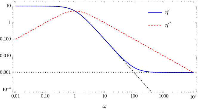
Figure 1: The dependence on the angular frequency $\omega$ of the linear viscoelastic moduli $\eta^{\prime}$ and $\eta^{\prime\prime}$ of the present model is typical of systems with a single relaxation time. The dissipative modulus $\eta^{\prime}$ is the sum of a plastic contribution (dot-dashed line), identical to the prediction of an upper-convected Maxwell model, and a constant viscous term (dotted line) given by $\eta$. The elastic modulus $\eta^{\prime\prime}$ grows linearly, displays the expected peak around $\omega=1/\tau_{\mathrm{r}}$, and then decays as $1/\omega$. In this example, we chose $\tau_{\mathrm{r}}=1$ s, $\kappa=10$ Pa, and $\eta=10^{-3}$ Pa s.

5 Stress growth after inception of steady flows

In this section, we analyze the evolution of the stress when a steady flow is suddenly imposed starting from a stress-free static condition. The constant strain rate is $\dot{\gamma}:=\sqrt{2\mathsf{D}:\mathsf{D}}$. The components of the extra stress are represented by the following time-dependent material coefficients

$$\eta_{\mathrm{eff}}^{+}(t;\tau_{\mathrm{r}},\kappa,\eta,\dot{\gamma}):=\frac{1}{\dot{\gamma}}\frac{{\mathsf{T}}:\hat{\mathsf{D}}}{\hat{\mathsf{D}}:\hat{\mathsf{D}}}\qquad\text{and}\qquad\Psi_{\mathrm{eff}}^{+}(t;\tau_{\mathrm{r}},\kappa,\eta,\dot{\gamma}):=\frac{2}{\dot{\gamma}^{2}}\frac{{\mathsf{T}}:\hat{{\mathsf{G}}}}{\hat{{\mathsf{G}}}:\hat{{\mathsf{G}}}},$$ (18)

where

$$\hat{\mathsf{D}}:=\frac{2}{\dot{\gamma}}\mathsf{D}\quad\text{and}\quad\hat{{\mathsf{G}}}:=\frac{1}{2}(\mathsf{A}\hat{\mathsf{D}}-\hat{\mathsf{D}}\mathsf{A}),\quad\text{having set }\mathsf{A}:=\begin{pmatrix}0&1\\ -1&0\end{pmatrix}\text{ for planar flows.}$$

Following Giusteri & Seto [10], we employ a definition of the material coefficients that is independent of the flow type, to be able to directly compare the results obtained in extensional and simple shear flows.

The definitions given in (18) coincide with the standard material functions (viscosity and first normal stress coefficient) in simple shear flows, but can be used to analyze any steady flow. Steady-state material functions will be determined as the long-time limit of $\eta_{\mathrm{eff}}^{+}$ and $\Psi_{\mathrm{eff}}^{+}$. We will find analytical expressions in planar and uniaxial extensional flows and then numerically study the case of simple shear.

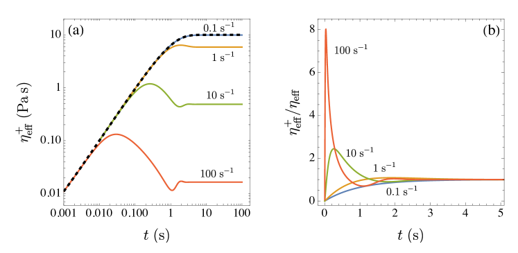
Figure 2: Stress overshoot after inception of steady shear is well captured together with a rate-dependent behavior. Looking at the time-evolution of $\eta_{\mathrm{eff}}^{+}$ for different values of the shear rate $\dot{\gamma}$ (curve labels), we see that in the low-rate regime, with $\dot{\gamma}\ll 1/\tau_{\mathrm{r}}$, the rate-dependence becomes negligible and $\eta_{\mathrm{eff}}^{+}$ converges to the extensional flow result (black dashed line in panel (a)). At high shear rates, $\dot{\gamma}\gtrsim 1/\tau_{\mathrm{r}}$, the growth of $\eta_{\mathrm{eff}}^{+}$ is hindered, it reaches a maximum at a strain $\dot{\gamma}t\approx 3$, and then decays toward a rate-dependent asymptotic value, with possibly a few oscillations. This behavior is even clearer by looking at the data normalized, in panel (b), by the steady value $\eta_{\mathrm{eff}}$. The values of material parameters are $\tau_{\mathrm{r}}=1$ s, $\kappa=10$ Pa, and $\eta=10^{-3}$ Pa s.

5.1 Planar extensional flow

In this case, the deformation map ${\bm{\varphi}}$, the deformation gradient $\mathsf{F}$, and the relaxed state $\mathsf{F}_{\mathrm{R}}$ are given by

$${\bm{\varphi}}(t,x,y)=\begin{pmatrix}e^{\frac{1}{2}\dot{\gamma}t}x\\ e^{-\frac{1}{2}\dot{\gamma}t}y\end{pmatrix},\qquad\mathsf{F}=\begin{pmatrix}e^{\frac{1}{2}\dot{\gamma}t}&0\\ 0&e^{-\frac{1}{2}\dot{\gamma}t}\end{pmatrix},\qquad\mathsf{F}_{\mathrm{R}}=\begin{pmatrix}e^{\frac{1}{2}\gamma_{\mathrm{R}}(t)}&0\\ 0&e^{-\frac{1}{2}\gamma_{\mathrm{R}}(t)}\end{pmatrix}.$$

The evolution equation for $\mathsf{F}_{\mathrm{R}}$ reduces to the scalar equation

$$\frac{\partial\gamma_{\mathrm{R}}}{\partial t}=\frac{1}{\tau_{\mathrm{r}}}(\dot{\gamma}t-\gamma_{\mathrm{R}}),$$ (19)

that, assuming the initial condition $\gamma_{\mathrm{R}}(0)=0$, leads to

$$\gamma_{\mathrm{R}}(t)=\dot{\gamma}\left(t-\tau_{\mathrm{r}}+\tau_{\mathrm{r}}e^{-t/\tau_{\mathrm{r}}}\right).$$ (20)

From this, we easily obtain

$$\log\mathsf{B}_{\mathrm{el}}=\tau_{\mathrm{r}}\dot{\gamma}\left(1-e^{-t/\tau_{\mathrm{r}}}\right)\begin{pmatrix}1&0\\ 0&-1\end{pmatrix}.$$ (21)

Recalling that in this case the deformation rate tensor is

$$\mathsf{D}=\frac{\dot{\gamma}}{2}\begin{pmatrix}1&0\\ 0&-1\\ \end{pmatrix},$$

we find

$$\eta_{\mathrm{eff}}^{+}(t;\tau_{\mathrm{r}},\kappa,\eta,\dot{\gamma})=\kappa\tau_{\mathrm{r}}\left(1-e^{-t/\tau_{\mathrm{r}}}\right)+\eta\qquad\text{and}\qquad\Psi_{\mathrm{eff}}^{+}(t;\tau_{\mathrm{r}},\kappa,\eta,\dot{\gamma})=0.$$ (22)

We stress that $\eta_{\mathrm{eff}}^{+}$ turns out to be independent of the shear rate $\dot{\gamma}$, and so is the steady-state apparent viscosity

$$\eta_{\mathrm{eff}}(\tau_{\mathrm{r}},\kappa,\eta):=\lim_{t\to+\infty}\eta_{\mathrm{eff}}^{+}(t;\tau_{\mathrm{r}},\kappa,\eta)=\kappa\tau_{\mathrm{r}}+\eta,$$

which is also identical to the zero-frequency dissipative modulus $\eta^{\prime}(0;\tau_{\mathrm{r}},\kappa,\eta)$. The normal stress coefficient $\Psi_{\mathrm{eff}}^{+}$ is rate-independent in a trivial way: it is identically zero in extensional flows due to symmetry reasons.

5.2 Uniaxial extensional flow

In uniaxial extensional flow the deformation map ${\bm{\varphi}}$ is given by

$${\bm{\varphi}}(t,x,y,z)=(e^{-\frac{\dot{\gamma}t}{4}}x,e^{-\frac{\dot{\gamma}t}{4}}y,e^{\frac{\dot{\gamma}t}{2}}z)^{\mathsf{T}},$$

and the deformation gradient $\mathsf{F}$ and the relaxed state $\mathsf{F}_{\mathrm{R}}$ are given by

$$\mathsf{F}=\begin{pmatrix}e^{-\dot{\gamma}t/4}&0&0\\ 0&e^{-\dot{\gamma}t/4}&0\\ 0&0&e^{\dot{\gamma}t/2}\\ \end{pmatrix},\qquad\mathsf{F}_{\mathrm{R}}=\begin{pmatrix}e^{-\gamma_{\mathrm{R}}/4}&0&0\\ 0&e^{-\gamma_{\mathrm{R}}/4}&0\\ 0&0&e^{\gamma_{\mathrm{R}}/2}\\ \end{pmatrix}.$$

The evolution equation for $\mathsf{F}_{\mathrm{R}}$ reduces again to (19) with solution (20). Since we obtain

$$\log\mathsf{B}_{\mathrm{el}}=\dot{\gamma}\tau_{\mathrm{r}}\left(1-e^{-t\tau_{\mathrm{r}}}\right)\begin{pmatrix}-1/2&0&0\\ 0&-1/2&0\\ 0&0&1\end{pmatrix}\qquad\text{and}\qquad\mathsf{D}=\frac{\dot{\gamma}}{2}\begin{pmatrix}-1/2&0&0\\ 0&-1/2&0\\ 0&0&1\end{pmatrix},$$

we eventually arrive at a result which is identical to the one obtained for planar extensional flows.

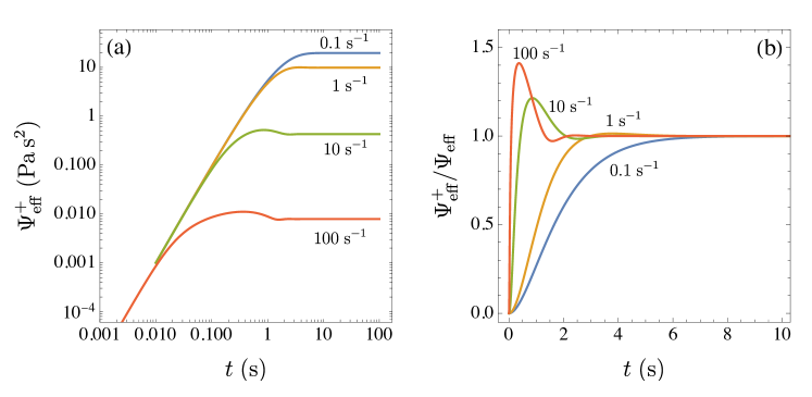
Figure 3: The first normal stress coefficient $\Psi_{\mathrm{eff}}^{+}$ is nonzero in simple shear and its growth after inception of steady shear is rate-dependent. At low rates ($\dot{\gamma}<<1/\tau_{\mathrm{r}}$) the rate-dependence disappears and the growth is monotonic, while for $\dot{\gamma}\gtrsim 1/\tau_{\mathrm{r}}$ we observe a short-time peak followed by a decay toward the rate-dependent steady value $\Psi_{\mathrm{eff}}$ (panel (a)). This behavior is emphasized in the data normalized by the steady value $\Psi_{\mathrm{eff}}$, shown in panel (b). The values of material parameters are $\tau_{\mathrm{r}}=1$ s, $\kappa=10$ Pa, and $\eta=10^{-3}$ Pa s.

5.3 Simple shear

For simple shear flows, the deformation map ${\bm{\varphi}}$ and the deformation gradient $\mathsf{F}$ are given by

$${\bm{\varphi}}(t,x,y,\dot{\gamma})=\begin{pmatrix}x+y\dot{\gamma}t\\ y\end{pmatrix}\qquad\text{and}\qquad\mathsf{F}=\begin{pmatrix}1&\dot{\gamma}t\\ 0&1\end{pmatrix},$$

but there is no reason to assume a specific shape for the relaxed state $\mathsf{F}_{\mathrm{R}}$, which must be determined by solving the evolution equation (4). This is a fully tensorial evolution equation that, generally, cannot be reduced to a scalar one. We then solve it numerically.

A very important consequence of the structure of equation (4) is that the eigenvectors of $\mathsf{B}_{\mathrm{el}}$ rotate over time and are different from those of $\mathsf{D}$. This gives rise to two important effects: the first normal stress coefficient is no longer zero and we observe a dependence of the material functions $\eta_{\mathrm{eff}}^{+}$ and $\Psi_{\mathrm{eff}}^{+}$ on the shear rate $\dot{\gamma}$. In the low-rate regime, with $\dot{\gamma}\ll 1/\tau_{\mathrm{r}}$, the rate-dependence becomes negligible and $\eta_{\mathrm{eff}}^{+}$ converges to the extensional flow result (22), which is also coincident with the prediction, for simple shear, of an upper-convected Maxwell model (though this would give a different result in extension). When, on the other hand, $\dot{\gamma}\gtrsim 1/\tau_{\mathrm{r}}$, the measured shear stress stems from a competition between the speed of the rotation of stress eigenvectors and that of the plastic relaxation. Essentially, the growth of $\eta_{\mathrm{eff}}^{+}$ is hindered, it reaches a maximum at a strain $\dot{\gamma}t\approx 3$, and then decays toward a rate-dependent asymptotic value, with possibly a few oscillations (see Figure 2). A similar behavior is followed by the normal stress coefficient $\Psi_{\mathrm{eff}}^{+}$ that shows a rate-independent growth for $\dot{\gamma}\ll 1/\tau_{\mathrm{r}}$ and a rate-dependent asymptotic value for $\dot{\gamma}\gtrsim 1/\tau_{\mathrm{r}}$ (see Figure 3). Our findings are qualitatively compatible with experimental data as can be seen by comparing them with Figures 3.4-7, 3.4-8, 3.4-9, and 3.4-10 of [3].

The steady state material functions $\eta_{\mathrm{eff}}$ and $\Psi_{\mathrm{eff}}$ display, in simple shear, a rate-dependent behavior of shear-thinning type (Figure 4). The effective viscosity decreases, for $\dot{\gamma}\gtrsim 1/\tau_{\mathrm{r}}$, from the low-rate value given by $\kappa\tau_{\mathrm{r}}+\eta$ to the asymptotic value set by $\eta$. We thus see that plastic dissipation dominates the low-rate material response. The effective normal stress coefficient, which is not influenced by the viscosity parameter $\eta$, simply decreases from its zero-rate value and vanishes asymptotically. Overall, the simple assumptions present in our model with constant parameters can reproduce qualitative features common to several viscoelastic fluids while providing an understanding of the underlying competition between elasticity, relaxation, and flow geometry that cannot be achieved by means of empirical data-fitting laws.

In this section, we treated simple shear as a two-dimensional flow. If, on the other hand, we view it as a planar but three-dimensional flow, a second normal stress coefficient becomes relevant for the characterization of the material. As long as the deformation remains planar, the present model assigns a vanishing stress in the third spatial direction. This implies that the second normal stress coefficient coincides always with $-\Psi_{\mathrm{eff}}/2$. The sign of this quantity is consistent with most measurements in the context of viscoelastic fluids, but the reported magnitude is typically significantly lower [11]. We believe that further consideration of how to capture experimental observations of second normal stress coefficients will be an important direction for future investigations.

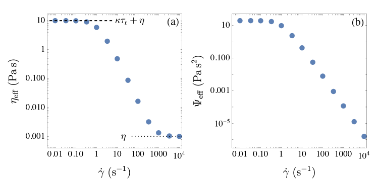
Figure 4: The rate dependence in simple shear of the steady-state material functions $\eta_{\mathrm{eff}}$ and $\Psi_{\mathrm{eff}}$ displays a shear-thinning behavior common to many viscoelastic fluids. The effective viscosity, in panel (a), interpolates between the zero-rate value, given by $\kappa\tau_{\mathrm{r}}+\eta$ (dashed line), and $\eta$ (dotted line), while the effective normal stress coefficient, in panel (b), simply decreases to zero. The values of material parameters are $\tau_{\mathrm{r}}=1$ s, $\kappa=10$ Pa, and $\eta=10^{-3}$ Pa s.

6 Stress relaxation after a sudden deformation

A fundamental parameter of our model is the relaxation time $\tau_{\mathrm{r}}$ and it can be directly related to stress relaxation experiments. We consider a material held in a static configuration after a very rapid homogeneous deformation. In the case of an extensional deformation, we can compute the time-dependent elastic stress by taking

$$\mathsf{F}=\begin{pmatrix}e^{\frac{1}{2}\gamma_{0}}&0\\ 0&e^{-\frac{1}{2}\gamma_{0}}\end{pmatrix},\qquad\mathsf{F}_{\mathrm{R}}=\begin{pmatrix}e^{\frac{1}{2}\gamma_{\mathrm{R}}(t)}&0\\ 0&e^{-\frac{1}{2}\gamma_{\mathrm{R}}(t)}\end{pmatrix}.$$

with $\gamma_{0}$ constant. The evolution equation for $\mathsf{F}_{\mathrm{R}}$ easily leads to $\gamma_{\mathrm{R}}(t)=\gamma_{0}(1-e^{-t/\tau_{\mathrm{r}}})$ and

$${\mathsf{T}}_{\mathrm{el}}=\kappa\log\mathsf{B}_{\mathrm{el}}=(\gamma_{0}-\gamma_{\mathrm{R}})\begin{pmatrix}1&0\\ 0&-1\end{pmatrix}=\kappa\gamma_{0}e^{-t/\tau_{\mathrm{r}}}\begin{pmatrix}1&0\\ 0&-1\end{pmatrix}.$$ (23)

From this, we clearly see that the stress decays exponentially with rate $1/\tau_{\mathrm{r}}$. By numerical integration of the evolution equation for $\mathsf{F}_{\mathrm{R}}$, we obtain the same decay also in the case of a simple shear deformation. Nevertheless, in simple shear the prefactor can depend nonlinearly on $\gamma_{0}$ for large initial strain. At this point, we have available several sets of experiments with which we can measure the values of the material parameters $\tau_{\mathrm{r}}$, $\kappa$, and $\eta$.

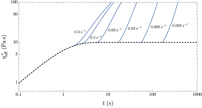
Figure 5: With a strain-dependent relaxation time we can capture polymeric jamming. The growth of the effective viscosity $\eta_{\mathrm{eff}}^{+}$ in uniaxial extension features a rate-independent segment (black dashed line) followed until the rate-dependent time $\gamma_{\mathrm{J}}/\dot{\gamma}$, after which we observe a fast increase (solid lines) due to the rapidly growing relaxation time. Values of $\dot{\gamma}$ label the different data curves. The values of model parameters for this example are $\tau_{\mathrm{r}}^{0}=1$ s, $\gamma_{\mathrm{J}}=0.5$, $\alpha=4$, $\kappa=10$ Pa, and $\eta=10^{-3}$ Pa s.

7 Polymeric jamming in uniaxial extension

The results of the previous sections show that part of the flow-type dependence of the material response, namely the shear-thinning behavior versus rate-independence in extensional flows, is not related to microscopic phenomena but rather to the rotation of the principal strains in simple shear (which in this context is non that simple, after all). Nevertheless, there are further differences, such as extensional thickening or the impossibility of reaching a steady state, that cannot be captured with the simplest constant-parameter model.

Here we propose a mechanism and a model that can explain some features of extensional rheology, focusing on uniaxial extension for definiteness. We argue that the typical experimental realization of uniaxial extension can lead, for some fluids, to the phenomenon of polymeric jamming. That is, molecular chains that are mostly elongated in one direction and, due to the confinement in filament stretching experiments, compressed in the orthogonal plane become progressively unable to relax. We do not expect a similar phenomenon in simple shear flows where confinement does not change over time. Note that this type of effect is not necessarily related to the bulk rheology of the material, but rather to its interaction with the experimental setup, meaning that it may not appear in large-scale extensional flows.

A very rough model for polymeric jamming can be set up by letting the relaxation time $\tau_{\mathrm{r}}$ depend on a measure of the total strain such as $\gamma(t)=\dot{\gamma}t$, which is obviously related to the filament shrinking. In particular, we fix a threshold $\gamma_{\mathrm{J}}>0$ and we assume that $\tau_{\mathrm{r}}=\tau_{\mathrm{r}}^{0}$, with $\tau_{\mathrm{r}}^{0}$ constant and finite, as long as $\gamma(t)<\gamma_{\mathrm{J}}$, whereas $\tau_{\mathrm{r}}=\tau_{\mathrm{r}}^{0}e^{\alpha(\gamma(t)-\gamma_{\mathrm{J}})}$ if $\gamma(t)\geq\gamma_{\mathrm{J}}$. Note that the energy balance (11) still applies to this model. The exponential growth of $\tau_{\mathrm{r}}$ is, at this stage, an arbitrary modelling choice to have the material approach a solid one ($\tau_{\mathrm{r}}=+\infty$) rather fast. It is possible to solve equation (19) analytically in the region with growing $\tau_{\mathrm{r}}$, but the expression of the solution is not quite informative, and numerical integration is equally effective. The parameter $\alpha>0$ determines the slope of the effective viscosity $\eta_{\mathrm{eff}}^{+}$ beyond the jamming strain. Indeed, with this model we predict a rate-independent behavior in the initial (rate-dependent) interval $[0,\gamma_{\mathrm{J}}/\dot{\gamma}]$, with $\eta_{\mathrm{eff}}^{+}(t)=\kappa\tau_{\mathrm{r}}^{0}(1-e^{-t/\tau_{\mathrm{r}}^{0}})+\eta$, followed by a fast increase, with a slope that looks approximately the same in log-scale for $\dot{\gamma}$ sufficiently small, and no steady state is attained. By choosing $\alpha=4$, we obtain a picture, in Figure 5, that is in striking qualitative agreement with Series PSII in Figure 3.5-2 of [3]. This provides a strong indication that our model can capture the mechanism behind the experimental observation.

8 A note on dimensionless numbers

In our presentation we preferred to make use of dimensional parameters for an easier link with measurable quantities. Nevertheless, it is important to identify dimensionless parameters that can help understanding the scaling behavior of our model. The most common dimensionless numbers related to viscoelastic fluids are the Deborah ($\mathit{De}$) and Weissenberg ($Wi$) numbers (see the note by Dealy [12] for a clear discussion of their definition). Clearly, they both compare the relaxation time $\tau_{\mathrm{r}}$ with a characteristic rate associated with the fluid flow and remain relevant also in our model. In fact, $\mathit{De}=1$ and $\mathit{Wi}=1$ mark important transition points in the frequency- and rate-dependence of the material functions, respectively. This can be seen from Figures 1 and 4, where the choice $\tau_{\mathrm{r}}=1$ s allows to view the plots as if the appropriate dimensionless numbers were on the horizontal axis.

Our model, in comparison with that of a Newtonian fluid, features two extra parameters, $\tau_{\mathrm{r}}$ and $\kappa$. Given that the former leads to $\mathit{De}$ or $\mathit{Wi}$, depending on the flow, we clearly need to introduce another dimensionless group. To quantify the overall relative importance between the plastic dissipation due to elasticity and viscous forces (with no reference to a specific flow) we can consider the quantity $(\kappa\tau_{\mathrm{r}}+\eta)/\eta$. This number is very useful in two ways: first, it describes the (log-scale) range within which the effective viscosity can vary; second, it represents the relative importance of plasticity with respect to viscosity in the material response observed at low values of $\mathit{De}$ in oscillatory flows. At high values of $\mathit{De}=\omega\tau_{\mathrm{r}}$, the dissipation is mostly viscous, plasticity does not intervene, and the material response is that of a viscoelastic solid.

The situation in flows with constant strain rate is more involved. First of all, we should stress that using the ratio of the first normal stress difference over the shear stress to measure the degree of elasticity or nonlinearity of the fluid is misleading. In fact, such a ratio becomes $\dot{\gamma}\Psi_{\mathrm{eff}}/\eta_{\mathrm{eff}}$, a quantity that is identically zero in extensional flows, irrespective of the presence of elastic stresses. We then consider the definition $\mathit{Wi}=\dot{\gamma}\tau_{\mathrm{r}}$ (independent of the flow type) and observe that, in extensional flows, $\mathit{Wi}$ is hardly relevant, since the stress growth and steady state are rate-independent. In simple shear, we can conclude that for large $\mathit{Wi}$ the behavior of the fluid is essentially viscous. This is due to the fact that a faster rotation of the principal directions of the elastic stress makes relaxation more efficient, leading to smaller values of the elastic strain and, consequently, stress.

9 Conclusions

We introduced a class of tensorial models aimed at describing viscoelastic materials. The cornerstones of this framework are an elastic stress that depends logarithmically on a suitable measure of strain and the choice of letting the elastic strain evolution emerge from two distinct evolution equations, one for the current deformation and the other for a tensorial descriptor of the elastically-relaxed state. While the former is a necessary kinematic relation between velocity and deformation, the latter involves constitutive choices that are based on arguments borrowed from solid plasticity. Our line of thought differs considerably form the classical Oldroyd’s approach. Even though we can derive an equation for a quantity akin to a conformation tensor, the objective rate entering its evolution is not a matter of choice, as it descends directly from the kinematic evolution of the current deformation gradient. We stress that, in our framework, viscoelastic fluids emerge as an interpolation between purely viscous fluids and solids, controlled by a relaxation time parameter ranging from zero (viscous fluid) to infinity (viscoelastic solid).

We have shown that a simple model with constant material parameters performs very well in reproducing the behavior of viscoelastic fluids observed in rheometric experiments. Moreover, it helps understanding the origin of the difference in extensional and shear rheology and the relative importance of viscous, elastic, and plastic effects. We did not address the matching with data for specific fluids, but rather aimed at highlighting the broad qualitative agreement with experiments. Another important feature of this model is that it avoids the erroneous prediction of an exponential growth of the elastic stress in extensional flows that sometimes arises in connection with elastic models of neo-Hookean type.

To approach the modelling of real fluids, it is important to consider the presence of multiple relaxation times. This can be done within our framework by letting the relaxation time parameter depend on other relevant quantities. We provide a first example of what can be achieved in this way by addressing a situation in which an abrupt change in the elastic response during uniaxial extension prevents the attainment of steady flows. Our findings suggest the presence of a phenomenon that can be described as a progressive polymeric jamming, in which the relaxation time diverges due to the experiment geometry. How to harness the freedom in modelling the relaxation time parameter to capture further rheological behaviors, such as viscoplastic yielding and softening, and describe different classes of complex fluids will be the subject of future research.

Authors’ contributions: G.G.G. conceived the model and M.A.H A. performed analytical and numerical computations. Both authors edited and revised the manuscript, and gave final approval for publication.

Acknowledgments: During the development of this research, the work of G.G.G. was partially supported by the National Group for Mathematical Physics (GNFM) of the Italian National Institute for Advanced Mathematics (INdAM).

References

- [1] J. G. Oldroyd. On the formulation of rheological equations of state. Proceedings of the Royal Society of London. Series A. Mathematical and Physical Sciences, 200(1063):523–541, 1950.
- [2] J. G. Oldroyd. Non-newtonian effects in steady motion of some idealized elastico-viscous liquids. Proceedings of the Royal Society of London. Series A. Mathematical and Physical Sciences, 245(1241):278–297, 1958.
- [3] R. B. Bird, R. C. Armstrong, and O. Hassager. Dynamics of polymeric liquids. Vol. 1: Fluid mechanics. John Wiley and Sons Inc., New York, NY, 1987.
- [4] N. Phan-Thien and N. Mai-Duy. Understanding viscoelasticity. Springer, 2013.
- [5] H. Giesekus. Die elastizität von flüssigkeiten. Rheologica Acta, 5:29–35, 1966.
- [6] H. Giesekus. A simple constitutive equation for polymer fluids based on the concept of deformation-dependent tensorial mobility. Journal of Non-Newtonian Fluid Mechanics, 11(1-2):69–109, 1982.
- [7] N. Phan-Thien and R. I. Tanner. A new constitutive equation derived from network theory. Journal of Non-Newtonian Fluid Mechanics, 2(4):353–365, 1977.
- [8] Antony N Beris. Continuum mechanics modeling of complex fluid systems following Oldroyd’s seminal 1950 work. Journal of Non-Newtonian Fluid Mechanics, 298:104677, 2021.
- [9] J. H. Snoeijer, A. Pandey, M. A. Herrada, and J. Eggers. The relationship between viscoelasticity and elasticity. Proceedings of the Royal Society A, 476(2243):20200419, 2020.
- [10] G. G. Giusteri and R. Seto. A theoretical framework for steady-state rheometry in generic flow conditions. Journal of Rheology, 62(3):713–723, 2018.
- [11] O. Maklad and R. J. Poole. A review of the second normal-stress difference; its importance in various flows, measurement techniques, results for various complex fluids and theoretical predictions. Journal of Non-Newtonian Fluid Mechanics, 292:104522, 2021.
- [12] J. M. Dealy. Weissenberg and Deborah numbers – their definition and use. Rheology Bulletin, 79(2):14–18, 2010.