Can supercooled phase transitions explain the gravitational wave background observed by pulsar timing arrays?

Abstract

Several pulsar timing array collaborations recently reported evidence of a stochastic gravitational wave background (SGWB) at nHz frequencies. Whilst the SGWB could originate from the merger of supermassive black holes, it could be a signature of new physics near the 100 MeV scale. Supercooled first-order phase transitions (FOPTs) that end at the 100 MeV scale are intriguing explanations, because they could connect the nHz signal to new physics at the electroweak scale or beyond. Here, however, we provide a clear demonstration that it is not simple to create a nHz signal from a supercooled phase transition, due to two crucial issues that should be checked in any proposed supercooled explanations. As an example, we use a model based on non-linearly realized electroweak symmetry that has been cited as evidence for a supercooled explanation. First, we show that a FOPT cannot complete for the required transition temperature of around 100 MeV. Such supercooling implies a period of vacuum domination that hinders bubble percolation and transition completion. Second, we show that even if completion is not required or if this constraint is evaded, the Universe typically reheats to the scale of any physics driving the FOPT. The hierarchy between the transition and reheating temperature makes it challenging to compute the spectrum of the SGWB.

I Introduction

The North American Nanohertz Observatory for Gravitational Waves (NANOGrav) recently detected a stochastic gravitational wave background (SGWB) for the first time with a significance of about $4\sigma$ NANOGrav:2023gor . This was corroborated by other pulsar timing array (PTA) experiments, including the Chinese Pulsar Timing Array (CPTA; Xu:2023wog ), the European Pulsar Timing Array (EPTA; Antoniadis:2023ott ), and the Parkes Pulsar Timing Array (PPTA; Reardon:2023gzh ). Although the background could originate from mergers of super-massive black holes (SMBHs; NANOGrav:2023hfp ; Ellis:2023dgf ), this explanation might be inconsistent with previous estimates of merger density and remains a topic of debate Casey-Clyde:2021xro ; Kelley:2016gse ; Kelley:2017lek . Thus, there is an intriguing possibility that the SGWB detected by NANOGrav could originate from more exotic sources NANOGrav:2023hvm . Indeed, many exotic explanations were proposed for an earlier hint of this signal NANOGrav:2020bcs ; NANOGrav:2021flc ; Bian:2020urb , or immediately after the announcement. These include non-canonical kinetic terms Yi:2021lxc , inflation Vagnozzi:2020gtf ; Benetti:2021uea ; Gao:2021lno ; Ashoorioon:2022raz ; Vagnozzi:2023lwo , first-order phase transitions (FOPTs; Nakai:2020oit ; Ratzinger:2020koh ; Xue:2021gyq ; Deng:2023seh ; Megias:2023kiy ), cosmic strings Blasi:2020mfx ; Ellis:2020ena ; Buchmuller:2020lbh ; Blanco-Pillado:2021ygr ; Bian:2022tju ; Samanta:2020cdk ; Wang:2023len ; Ellis:2023tsl , domain walls Ferreira:2022zzo ; King:2023cgv , primordial black holes Franciolini:2023pbf , primordial magnetic fields Li:2023yaj , axions and ALPs Ramberg:2020oct ; Ratzinger:2020koh ; Inomata:2020xad ; Sakharov:2021dim ; Kawasaki:2021ycf ; Guo:2023hyp ; Kitajima:2023cek ; Yang:2023aak , QCD Neronov:2020qrl ; Bai:2023cqj , and dark sector models Addazi:2020zcj ; Li:2021qer ; Borah:2021ocu ; Borah:2021ftr ; Freese:2022qrl ; Freese:2023fcr ; Han:2023olf ; Fujikura:2023lkn ; Zu:2023olm ; Han:2023olf .

The nanohertz (nHz) frequency of the signal indicates that any new physics explanation should naturally lie at around 100 MeV. If there are new particles around the MeV scale there are constraints from cosmology Foot:2014uba ; Bai:2021ibt ; Bringmann:2023opz ; Madge:2023cak as any new particles must not significantly alter the number of relativistic degrees of freedom Giovanetti:2021izc ; Planck:2018vyg , must not inject energy e.g. from particle decays that could spoil Big Bang nucleosynthesis (BBN) and distort the cosmic microwave background (CMB), and must not lead to an overabundance of dark matter (DM). In any case, there are constraints from laboratory experiments, such as fixed-target experiments, $B$-factories and high-energy particle colliders. These constraints may weaken if the new particles are sequestered in a dark sector, though could be important Bai:2013xga if one wishes to connect the dark sector to the Standard Model (SM).

It is conceivable, however, that new physics at characteristic scales far beyond the MeV scale could be responsible for a nHz signal. This could happen, for example, if a FOPT (see Refs. Caprini:2015zlo ; Caprini:2019egz ; Athron:2023xlk for reviews) starts at a temperature above the $100\,\text{MeV}$ scale but ends at the MeV scale due to supercooling. That is, the Universe remains in a false vacuum (a local minimum of the scalar potential) until the MeV scale because a transition to the true vacuum (the global minimum) is suppressed. A SGWB would be produced by percolation of bubbles of true vacuum. This was previously considered in the context of the electroweak phase transition Kobakhidze:2017mru ; Witten:1980ez ; Iso:2017uuu ; Arunasalam:2017ajm ; vonHarling:2017yew ; Baratella:2018pxi ; Bodeker:2021mcj ; Sagunski:2023ynd and was discussed as a possible new physics explanation by NANOGrav NANOGrav:2023hvm ; NANOGrav:2021flc . Supercooling could help new physics explanations evade constraints on MeV scale modifications to the SM and connect a nHz signal to new physics and phenomenology at the electroweak scale or above. For example, a scalar cubic coupling driving a supercooled FOPT Kobakhidze:2017mru could be observable through Higgs boson pair production at the Large Hadron Collider (LHC; ATLAS:2022jtk ).

In this work, however, we raise two difficulties with supercooled FOPTs. We explicitly demonstrate that these difficulties rule out one of the earliest models that was constructed to explain a nHz GW signal through a supercooled FOPT Kobakhidze:2017mru . This model was prominently cited as a viable example NANOGrav:2023hvm ; NANOGrav:2021flc . The difficulties are that, firstly, supercooled FOPTs that reach nucleation may still struggle to complete Athron:2022mmm and requiring completion places stringent limits on the viable parameter space Balazs:2023kuk . We show for the model proposed in Ref. Kobakhidze:2017mru that requiring the phase transition completes places a lower bound on the transition temperature, or more precisely the percolation temperature, and that the phase transition does not complete for the low temperatures associated with a nHz signal. This finding is consistent with brief remarks in Ref. Ellis:2018mja and, as mentioned there, similar to the graceful-exit problem in old inflation Guth:1982pn . Secondly, even if the completion criteria are ignored or can be evaded, the energy released by the phase transition reheats the Universe to about the new physics scale Madge:2023cak . The resulting hierarchy between the percolation and reheating temperatures makes it challenging to compute the SGWB spectrum.

II Cubic potential and Benchmarks

We consider a modification to the SM Higgs potential to include a cubic term,

$$V_{0}(r)=-\frac{\mu^{2}}{2}r^{2}+\frac{\kappa}{3}r^{3}+\frac{\lambda}{4}r^{4}.$$ (1)

Details of the model and the radiative and finite-temperature corrections included are described in Appendix A.1.

We consider two benchmark points to highlight the challenges of fitting a nHz signal with this cubic potential. These benchmarks are selected to probe two criteria: 1) realistic percolation, that is, that the physical volume of the false vacuum is decreasing at the onset of percolation (see eq. 26); and 2) having a completion temperature (see eq. 21). These benchmarks are:

$$\text{BP1: }\kappa =-116.81\,\text{GeV},$$ (2)

$$\text{BP2: }\kappa =-117.56\,\text{GeV}.$$ (3)

BP1 resulted in the most supercooling for which the transition satisfies both criteria, though fails to supercool to sub-GeV temperatures. For $\kappa$ just below $-116.81\,\text{GeV}$ we find that percolation is unrealistic by eq. 26 even though there is a completion temperature by eq. 21. BP2 resulted in stronger supercooling with a percolation temperature of 100 MeV; however, the transition did not complete. Although BP2 was chosen so that percolation was estimated to begin at 100 MeV according to the usual condition, we find that the space between bubbles continues to expand below 100 MeV. Thus, despite a nominal percolation temperature, both percolation and completion could be unrealistic in BP2. Without significant percolation of bubbles, the phase transition would not generate a SGWB. We discuss the results in the next section, with further details of the analysis left to the appendices.

III Challenges

III.1 Challenge 1 — completion

A possible strategy for achieving a peak frequency at the nHz scale is to consider a strongly supercooled phase transition, where bubble percolation is delayed to below the GeV scale and percolation is defined by $P_{f}(T_{p})=0.71$. However, in many models, a first-order electroweak phase transition has bubbles nucleating at around the electroweak scale. There is then an extended period of bubble growth and expansion of space. If bubbles grow too quickly compared to the expansion rate of the Universe, the bubbles will percolate before sufficient supercooling. Yet if bubbles grow too slowly the transition may never complete due to the space between bubbles inflating Turner:1992tz ; Ellis:2018mja ; Athron:2022mmm ; this effect can cause both the realistic percolation condition eq. 26 and the condition for a completion temperature to fail. Thus, while it is possible to tune model parameters to achieve percolation at sub-GeV temperatures, completion of the transition becomes less likely as supercooling is increased. We define the completion temperature $T_{f}$ as the temperature for which false vacuum fraction $P_{f}$ is 1%; that is, $P_{f}(T_{f})=0.01$. See section A.2 for details.

We find that completion is impossible for the cubic potential if $T_{p}\lesssim 1\,\text{GeV}$. The same arguments apply to the models considered in Ref. Athron:2022mmm . In the cubic potential, strong supercooling implies a Gaussian bubble nucleation rate peaking at $T_{\Gamma}\sim 50\,\text{GeV}$. Percolation at say $T_{p}\sim 1\,\text{GeV}$ and completion shortly after implies that the false vacuum fraction must drop sharply around $T_{p}$. Because $T_{\Gamma}\gg T_{p}$, we must have $P_{f}\approx 1$ until $T\sim T_{p}$, otherwise the influx of nucleated bubbles would quickly percolate. However, in the cubic potential, strong supercooling means that the false vacuum fraction decreases slowly over a large range of temperatures. This is because delayed percolation requires bubbles to slowly take over the Universe. Consequently, completion after the onset of percolation is also slow. This is demonstrated in fig. 1.

In Ref. NANOGrav:2023hvm , the cubic potential is suggested as a candidate model for a strongly supercooled phase transition that could explain the detected SGWB. The Universe was assumed to be radiation dominated in the original investigation Kobakhidze:2017mru of detecting GWs from the cubic potential with PTAs. However, a more careful treatment of the energy density during strong supercooling shows that the Universe becomes vacuum dominated Ellis:2018mja . This leads to a period of rapid expansion that hinders bubble percolation and completion of the transition. In fact, one must check not only that $P_{f}<0.01$ eventually, but also that the physical volume of the false vacuum is decreasing at $T_{p}$ Turner:1992tz ; Ellis:2018mja ; Athron:2022mmm (again see section A.2 for details).

We note that many studies still use the nucleation temperature $T_{n}$ as a reference temperature for GW production. As argued in Ref. Athron:2022mmm , the nucleation temperature is not an accurate predictor of GW production; the percolation temperature should be used instead. Figure 1 demonstrates the large difference between $T_{n}$ and $T_{p}$ in supercooled phase transitions. In BP1 the difference is $\mathcal{O}(10\,\mathrm{GeV})$. In BP2 there is no nucleation temperature — one might be tempted to assume GWs cannot be produced because of this. However, percolation and completion are possible even without a nucleation temperature Athron:2022mmm . Another large source of error is the use of $\beta/H$ for estimating the timescale of the transition. The mean bubble separation can be used instead as described in section A.3.

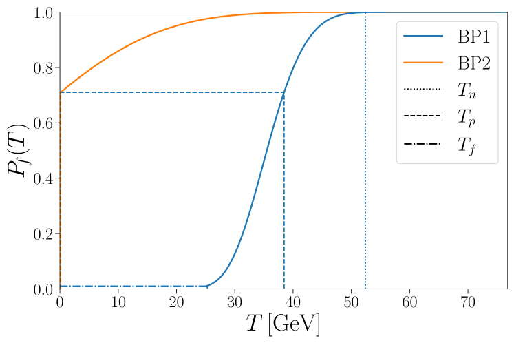
Figure 1: The false vacuum fraction as a function of temperature for BP1 (blue, right-most solid curve) and BP2 (orange, left-most solid curve). The nucleation (dotted), percolation (dashed) and completion (dash-dotted) temperatures are shown for both benchmark points. However, BP2 only has a percolation temperature, which is at $T_{p}\approx 100\,\text{MeV}$.

III.2 Challenge 2 — reheating

Even if the completion constraints can be avoided, a second issue was recently observed Madge:2023cak . Whilst strong supercooling can lower the percolation temperature down to $T_{p}\approx 100\,\text{MeV}$ as in BP2 or even lower, the energy released from the phase transition reheats the plasma, creating a hierarchy $T_{\text{reh}}\gg T_{p}$. Indeed, the reheating and percolation temperatures are approximately related by Ellis:2018mja

$$T_{\text{reh}}\simeq(1+\alpha)^{1/4}\,T_{p},$$ (4)

such that the substantial latent heat in a strongly supercooled transition, $\alpha\gg 1$, implies that $T_{\text{reh}}\gg T_{p}$. Ref. Madge:2023cak approximates the latent heat by the free energy difference ($\Delta V$) divided by radiation energy density and shows that in the Coleman-Weinberg model the latent heat is so large that the Universe reheats well above the percolation temperature and back to the scale of new physics.

A simple scaling argument suggests that this observation — that supercooled FOPTs reheat to the scale of new physics, $M$ — is generic. The new physics creates a barrier between minima so we expect $\Delta V\sim M^{4}$ and because the radiation energy density goes like $T_{p}^{4}$, we expect the latent heat may go like $\alpha\sim\frac{M^{4}}{T_{p}^{4}}$. This leads to

$$T_{\text{reh}}\sim\left(\frac{M^{4}}{T_{p}^{4}}\right)^{\frac{1}{4}}T_{p}=M.$$ (5)

It is possible this scaling can be avoided by fine-tuning terms to achieve $T_{\text{reh}}\ll M$ if $\Delta V\ll M^{4}$.

This argument, however, relies on the simple approximation of the reheating temperature in eq. 4 and crude dimensional analysis. We now confirm that this problem exists and is unavoidable in a careful analysis of the example model we consider. This careful treatment is general and can be used in other models. We assume that the reheating occurs instantaneously around the time of bubble percolation, and use conservation of energy so that the reheating temperature can be obtained from Athron:2023ts ; Athron:2022mmm

$$\rho(\phi_{f}(T_{p}),T_{p})=\rho(\phi_{t}(T_{\text{reh}}),T_{\text{reh}}),$$ (6)

where $\phi_{f}$ and $\phi_{t}$ are the false and true vacua, respectively, and $\rho$ is the energy density. For BP1, the percolation temperature is $T_{p}\approx 38.5\,\text{GeV}$, and the transition completes and reheats the Universe to $T_{\text{reh}}\approx 44.8\,\text{GeV}$. The reheating temperature exceeds the percolation temperature due to the energy released from the supercooled phase transition, though they remain of the same order of magnitude. For BP2, however, the percolation temperature drops to $T_{p}\approx 100\,\text{MeV}$, whereas the reheating temperature is $T_{\text{reh}}\approx 36.0\,\text{GeV}$; more than two orders of magnitude larger.

We show the behavior of the reheating temperature as a function of percolation temperature in fig. 2. These results come from a scan over $\kappa\in[-117.558\,\text{GeV},-116.800\,\text{GeV}]$. We clearly see that the reheating temperature tends towards a constant value $T_{\text{reh}}\approx 36\,\text{GeV}$ for $T_{p}\to 0$. As we now discuss, the fact that $T_{\Gamma}\sim T_{\text{reh}}\gg T_{p}$ breaks assumptions typically made when computing the SGWB.

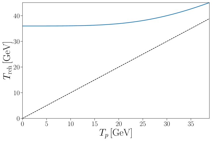
Figure 2: The reheating temperature $T_{\text{reh}}$ against percolation temperature $T_{p}$ as $\kappa$ varied. The dashed black line corresponds to $T_{\text{reh}}=T_{p}$. We see that $T_{\text{reh}}\gtrsim 36\,\text{GeV}$ even when $T_{p}\to 0$. See the main text for details.

III.3 Gravitational Wave Spectra

The frequencies of a SGWB created at a percolation temperature $T_{p}$ would be redshifted from the reheating temperature $T_{\text{reh}}$ to the current temperature $T\simeq 2.725\,\text{K}$ (for a review, see section 6.2 of Ref. Athron:2023xlk ). From the peak frequency equations (e.g. eq. 52) and the frequency redshift equation assuming radiation domination (see Ref. Athron:2023xlk ), the peak frequency of the SGWB today should be

$$f_{p}\approx 10\,\text{nHz}\,\left(\vphantom{\frac{f_{\text{peak}}|_{T=T_{p}}}{H_{*}}}\frac{g_{*}(T_{\text{reh}})}{100}\right)^{\!\frac{1}{6}}\left(\vphantom{\frac{f_{\text{peak}}|_{T=T_{p}}}{H_{*}}}\frac{T_{\text{reh}}}{100\,\text{MeV}}\right)\left(\frac{1}{R_{*}H(T_{\text{reh}})}\right),$$ (7)

where $R_{*}$ is the mean bubble separation, $H$ is the Hubble parameter and $g_{*}$ is the number of effective degrees of freedom. In the absence of supercooling we anticipate that $T_{\text{reh}}\sim T_{p}$, such that $R_{*}H(T_{\text{reh}})\sim R_{*}H(T_{p})$ and since the bubbles would not have a long time to grow $R_{*}H(T_{p})\lesssim 1$. Thus, in the absence of supercooling, we expect $T_{p}\sim 100\,\text{MeV}$ to lead to a $\sim 10\,\text{nHz}$ signal.

In this cubic model, however, $T_{p}\sim 100\,\text{MeV}$ requires strong supercooling, so we now consider an analysis more appropriate for this scenario. At the time of the phase transition the peak frequency $f_{p,*}$ is set by the mean bubble separation $R_{*}$ via $f_{p,*}\sim 1/R_{*}$ Caprini:2015zlo . Using the frequency redshift equation (40), the peak frequency of the SGWB today scales as

$$f_{p}\sim\frac{1\,\text{GeV}}{R_{*}(T_{p})s_{t}(T_{\text{reh}})^{1/3}},$$ (8)

where $s_{t}$ is the true vacuum entropy density (see the appendices for further details). Because radiation domination is a valid assumption in the true vacuum, the entropy density scales as $s_{t}(T)\sim T^{3}$.

One can show that $R_{*}\sim 1\,\text{GeV}/(T_{\Gamma}T_{p}N^{1/3})$ if bubbles nucleate simultaneously at $T_{\Gamma}$, where $N$ is the total number of bubbles nucleated per Hubble volume throughout the transition. Combining this with eq. 8, we obtain

$$f_{p}\sim T_{p}\left(\frac{T_{\Gamma}N^{\frac{1}{3}}}{T_{\text{reh}}}\right).$$ (9)

Numerically, we find that $N^{\frac{1}{3}}$, $T_{\Gamma}$ and $T_{\text{reh}}$ – and thus the right-most factor — depend only weakly on the amount of supercooling (see fig. 2). Thus, for supercooling we find the relationship $f_{p}\sim T_{p}$. This suggests that one can obtain an arbitrarily low peak frequency by fine-tuning the percolation temperature.

In the cubic model, these arguments are surprisingly accurate. Indeed, we find numerically that

$$\frac{1}{R_{*}H(T_{\text{reh}})}\simeq 1.1\,\left(\frac{T_{p}}{T_{\text{reh}}}\right)\left(\frac{T_{\Gamma}N^{\frac{1}{3}}}{T_{\text{reh}}}\right).$$ (10)

Assuming radiation domination in the true vacuum for $H(T_{\text{reh}})$ and that $g_{*}\approx 100$, eqs. 10 and 7 lead to

$$f_{p}\approx 10\,\text{nHz}\,\left(\vphantom{\frac{N^{\frac{1}{3}}}{T_{\text{reh}}^{2}}}\frac{T_{p}}{100\,\text{MeV}}\right)\left(\frac{T_{\Gamma}N^{\frac{1}{3}}}{T_{\text{reh}}}\right),$$ (11)

in agreement with the scaling anticipated in eq. 9. The right-most factor in eqs. 10 and 11 is $\mathcal{O}(1)$ and approximately independent of the amount of supercooling. Thus, to achieve a redshifted peak frequency of $10\,\text{nHz}$, we require $T_{p}\approx 100\,\text{MeV}$.

Comparing eq. 11 with the result in the absence of supercooling eq. 7, supercooling and subsequent substantial reheating redshift the frequency more than usual. However, assuming radiation domination eq. 10 leads to

$$R_{*}H(T_{p})\approx\frac{T_{\Gamma}}{T_{p}}.$$ (12)

This increase in bubble radius caused by the delay between nucleation and percolation partially offsets the impact of additional redshifting.

Our findings are contrary to the claim in Refs. Ellis:2018mja ; Madge:2023cak that reheating makes it difficult to reach GW frequencies relevant for PTAs. However, we do agree with the finding in Ref. Ellis:2018mja that completion poses an issue for nHz GW signals in this model. As found in section III.1, a percolation temperature of $T_{p}=100\,\text{MeV}$ would not result in a successful transition. Not only would the majority of the Universe remain in the false vacuum even today, the true vacuum bubbles would not actually percolate due to the inflating space between the bubbles.

We now consider the SGWB predictions. We take great care in our predictions. For example, we use the pseudotrace Giese:2020znk to avoid assumptions about the speed of sound and the equation of state that can break down in realistic models. We also use the mean bubble separation rather than proxy timescales derived from the bounce action that are invalid for strongly supercooled phase transitions. A full description of our treatment is given in sections A.3 and A.5.

In this model we find that the bubbles mostly nucleate at temperatures around $T_{\Gamma}\sim 50\,\text{GeV}$. We thus expect that friction from the plasma is sufficient to prevent runaway bubble walls, despite the large pressure difference. This implies that the SGWB from bubble collisions is negligible and that all the available energy goes into the fluid, resulting in a SGWB from sound waves and turbulence.

In fig. 3 we show the predicted SGWB spectrum for both BP1 (upper panel; the model with maximal supercooling while guaranteeing completion) and BP2 (lower panel; the model with percolation at 100 MeV but no completion). The peak frequencies are about $5\times 10^{4}\,\text{nHz}$ and $16\,\text{nHz}$ for BP1 and BP2, respectively. BP1 represents the lowest peak frequency that can be obtained for realistic scenarios in this model because for lower percolation temperatures the transition does not complete. Thus this model cannot explain the nHz signal observed by PTA experiments despite various optimistic statements from the literature. For comparison we show the SGWB prediction if one were to assume vacuum transitions (dotted grey curves). This assumption is not realistic for this model and in any case does not result in agreement with the observed spectrum.

If one ignores the completion requirement, BP2 shows that the peak frequency can be reduced to match the nHz signal observed by PTA experiments, though the amplitude is several orders of magnitude too high. Caution should be taken interpreting the SGWB predictions for such strong supercooling because it is well beyond what has been probed in simulations. Besides, despite a nominal percolation temperature, bubbles are not expected to percolate in BP2 because the false vacuum between them is inflating. Without percolation, GWs would not be generated.

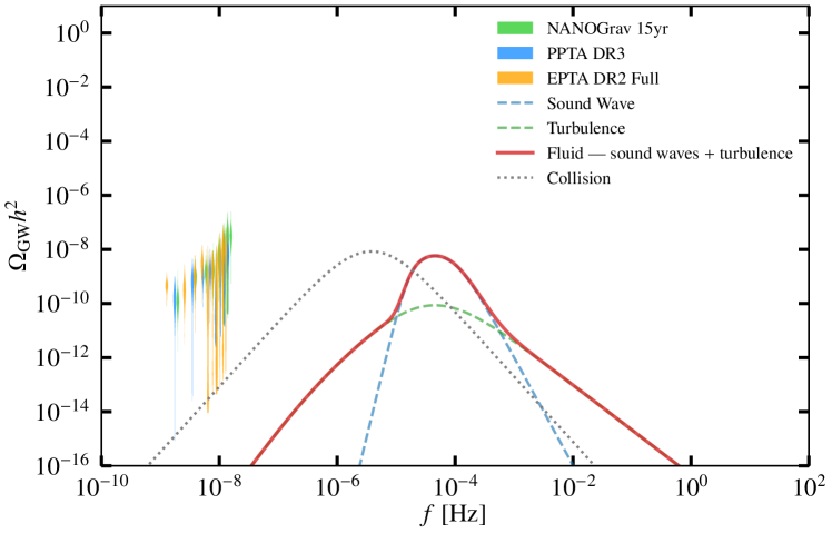
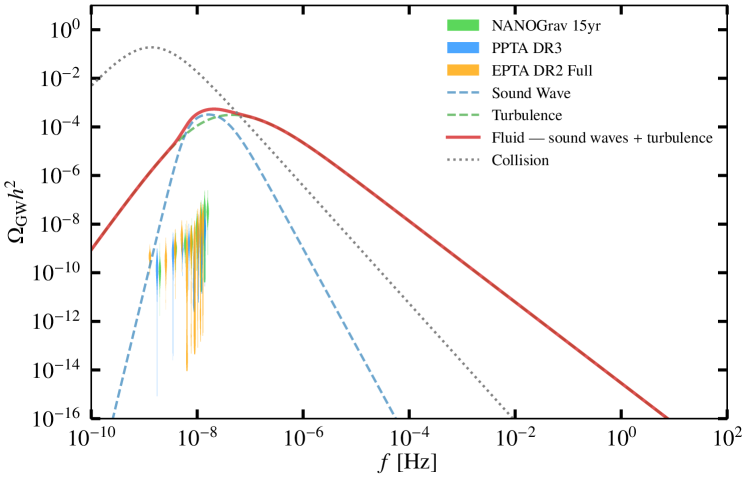
Figure 3: The SGWB from BP1 (top panel; strongest supercooling for which the FOPT completed) and BP2 (bottom panel; strongest supercooling for which the percolation temperature could be computed) fail to match the observations by PTA experiments (violins). Our BPs predict a non-vacuum transition in which all available energy goes into the fluid, such that total SGWB (solid red) is the sum of contributions from sound waves (dashed blue) and turbulence (dashed green). For comparison, we show a vacuum transition where bubble collisions are the sole source of GWs (dotted grey).

IV Conclusions

Supercooled FOPTs are an intriguing explanation of the nHz SGWB recently observed by several PTAs, as they could connect a nHz signal to phenomenology and experiments at the electroweak scale. Indeed, they were mentioned as a possibility NANOGrav:2023gor ; NANOGrav:2023hvm . However, we demonstrate that there are two major difficulties in supercooled explanations. First, completion of the transition is hindered by vacuum domination. We demonstrate that this rules out the possibility of explaining the PTA signal in the supercooling model mentioned as a prototypical example in Ref. NANOGrav:2023gor ; NANOGrav:2023hvm .

Second, the Universe typically reheats to the scale of any physics driving the transition. This makes it challenging to compute the SGWB spectrum because factors involving ratios of the reheat, nucleation and percolation temperatures — often implicitly neglected — must be carefully included in fit formulae. In any case, the predictions are questionable because the thermal parameters in these scenarios are well beyond those in hydrodynamical simulations on which fit formulae are based. We anticipate that these issues are quite generic and they should be carefully checked in any supercooled explanation.

Appendix A Predicting gravitational waves

In this appendix, we summarize our calculations for the phase transition and GW spectra. First, we sepcify the model and the effective potential we used, then we describe the analysis of the phase transition. We then give a detailed description of how we determine the relevant thermal parameters and the red shift factors for the peak amplitude and peak frequency for gravitational waves. Finally, we provide an outline of our fitting models for sound waves, turbulence, and collisions in GW spectra.

A.1 Effective Potential

Following Ref. Kobakhidze:2016mch ; Kobakhidze:2017mru , we construct a simple model that falls under the category of non-linearly realized electroweak symmetry. The SM Higgs doublet belongs to the coset group $G_{c}=\textit{SU}(2)_{L}\times U(1)_{Y}/U(1)_{\text{EM}}$ and can be expressed as

$$H(x)=\frac{r(x)}{\sqrt{2}}e^{i\theta^{i}(x)T^{i}}\begin{pmatrix}{0}\\ {1}\end{pmatrix},$$ (13)

where $i=1-3$. The Higgs boson is a singlet field in the SM, denoted as $r(x)\sim(1,1)_{0}$, and the fields $\theta^{i}(x)$ correspond to three would-be Goldstone bosons. The physical Higgs boson, $h$, is a fluctuation in $r$ around the vacuum expectation value of electroweak symmetry breaking, that is, $r=\langle r\rangle+h$, where $\langle r\rangle=v=246\,\text{GeV}$.

The general tree-level Higgs potential for the SM singlet field, $r$, can be written as

$$V_{0}(r)=-\frac{\mu^{2}}{2}r^{2}+\frac{\kappa}{3}r^{3}+\frac{\lambda}{4}r^{4}.$$ (14)

We add zero- and finite-temperature one-loop Coleman-Weinberg corrections to the tree-level potential,

$$V(r,T)=V_{0}(r)+[V_{\text{CW}}(r)+V_{T}(r,T)]|_{m_{i}^{2}\rightarrow m_{i}^{2}+\Delta_{T}},$$ (15)

and we replace all scalar and longitudinal gauge boson masses $m_{i}^{2}$ with the thermal masses $m_{i}^{2}+\Delta_{T}$ (evaluated at lowest order), such that we are using the Parwani method Parwani:1991gq for Daisy resummation to address infrared divergences. The formulas for $V_{\text{CW}}(r)$ and $V_{T}(r,T)$ and the thermal masses can be found in the Appendix of Ref. Kobakhidze:2017mru . We apply Boltzmann suppression factors $e^{-m^{2}/T^{2}}$ to the Debye corrections as discussed in section A.3. There are, of course, other possible models with supercooled FOPTs, including the classic Coleman-Weinberg model Coleman:1973jx .

The model parameters, namely $\mu$, $\kappa$, and $\lambda$, are constrained by the tadpole and on-shell mass conditions,

$$\left.\frac{dV}{dr}\right|_{r=v}=0,\quad\quad\left.\frac{d^{2}V}{dr^{2}}\right|_{r=v}=m^{2}_{h},$$ (16)

where $m_{h}\simeq 125\,\text{GeV}$. We use them to eliminate $\mu^{2}$ and $\lambda$ at the one-loop level through

$$\mu^{2} =\frac{1}{2}\left(m_{h}^{2}+\kappa v+\frac{3}{v}\left.\derivative{V_{\text{CW}}}{r}\right|_{v}-\left.\derivative[2]{V_{\text{CW}}}{r}\right|_{v}\right),$$ (17a)

$$\lambda =\frac{1}{2v^{2}}\left(m_{h}^{2}-\kappa v+\frac{1}{v}\left.\derivative{V_{\text{CW}}}{r}\right|_{v}-\left.\derivative[2]{V_{\text{CW}}}{r}\right|_{v}\right).$$ (17b)

This requires an iterative procedure starting with the tree-level tadpole equations and repeatedly using one-loop extraction until convergence. This leaves the cubic coupling $\kappa$ as the only free parameter. This cubic term creates a barrier between minima in the potential and can lead to supercooling. The remaining cubic coupling $\kappa$ creates a barrier between minima in the potential and can lead to supercooling. The requirement that the potential must be bounded from below ensures that $\lambda>0$. On the other hand, by convention so that $\langle r\rangle>0$, we choose $\kappa<0$.

In addition to the particles stated in the Appendix of Ref. Kobakhidze:2017mru , we add radiative corrections from all remaining quarks and the muon and tau. The omitted states are always so light that we can treat them as radiation. We therefore account for $81$ effective degrees of freedom in the one-loop and finite-temperature corrections, leaving $25.75$ degrees of freedom from light particles that we treat as pure radiation. Thus we add a final term to the effective potential:

$$V_{\text{rad}}(T)=-\frac{\pi^{2}}{90}g^{\prime}_{*}T^{4},$$ (18)

where $g^{\prime}_{*}=106.75-81=25.75$.

A.2 Phase transition analysis

We use PhaseTracer Athron:2020sbe to determine the phase structure (see ref. Athron:2022jyi for a discussion of uncertainties) and TransitionSolver Athron:2023ts to evaluate the phase history and extract the GW signal. The particle physics model considered in this study has at most one first-order phase transition, making phase history evaluation a simple matter of analyzing the single first-order phase transition. We use a modified version of CosmoTransitions Wainwright:2011kj to calculate the bounce action during transition analysis.

TransitionSolver tracks the false vacuum fraction Athron:2022mmm

$$P_{f}(T)=\exp\left[-\frac{4\pi}{3}v_{w}^{3}\int_{T}^{T_{c}}\frac{\Gamma(T^{\prime})dT^{\prime}}{T^{\prime 4}H(T^{\prime})}\left(\int_{T}^{T^{\prime}}\!\frac{dT^{\prime\prime}}{H(T^{\prime\prime})}\right)^{\!3}\right]$$ (19)

as a function of temperature, where $v_{w}$ is the bubble wall velocity, $\Gamma$ is the bubble nucleation rate, $H$ is the Hubble parameter, and $T_{c}$ is the critical temperature at which the two phases have equal free-energy density. This allows us to evaluate the GW power spectrum at the onset of percolation. Percolation occurs when the false vacuum fraction falls to $71\%$ doi:10.1063/1.1338506 ; LIN2018299 ; LI2020112815 . Thus we define the percolation temperature, $T_{p}$, through

$$P_{f}(T_{p})=0.71.$$ (20)

This temperature will be used as the reference temperature for GW production. Additionally, we define the completion (or final) temperature, $T_{f}$, through

$$P_{f}(T_{f})=0.01,$$ (21)

as an indication of the end of the phase transition.

The quantities in eq. 19 are estimated as follows. The bubble wall velocity $v_{w}$ is typically ultra-relativistic in the strongly supercooled scenarios we consider here, so we take $v_{w}\approx 1$. The bubble nucleation rate is estimated as Linde:1981zj

$$\Gamma(T)=T^{4}\!\left(\frac{S(T)}{2\pi}\right)^{\!\!\frac{3}{2}}\exp(-S(T)),$$ (22)

where $S(T)$ is the bounce action. The Hubble parameter

$$H(T)=\sqrt{\frac{8\pi G}{3}\rho_{\text{tot}}(T)}$$ (23)

depends on the total energy density Athron:2022mmm

$$\rho_{\text{tot}}(T)=\rho_{f}(T)-\rho_{\text{gs}},$$ (24)

and $G=6.7088\!\times\!10^{-39}\,\text{GeV}^{-2}$ is Newton’s gravitational constant Wu:2019pbm . The energy density of phase $\boldsymbol{\phi}_{i}$ is given by Espinosa:2010hh

$$\rho_{i}(T)=V(\boldsymbol{\phi}_{i},T)-T\left.\partialderivative{V}{T}\right|_{\boldsymbol{\phi}_{i}(T)},$$ (25)

where $V(\boldsymbol{\phi}_{i},T)$ is the effective potential. The subscript $f$ in eq. 24 denotes the false vacuum and gs denotes the zero-temperature ground state of the potential. Finally, the transition is analysed by evaluating the false vacuum fraction eq. 19 starting near the critical temperature and decreasing the temperature until the transition completes. We define completion to be when $P_{f}(T_{f})=0.01$, and further check that the physical volume of the false vacuum is decreasing at $T_{p}$ Turner:1992tz ; Athron:2022mmm ; that is,

$$3+T_{p}\left.\derivative{\mathcal{V}_{t}^{\text{ext}}}{T}\right|_{T_{p}}<0,$$ (26)

where $-\mathcal{V}_{t}^{\text{ext}}$ is the exponent in eq. 19. This condition was empirically determined to be the strongest completion criterion of those considered in Ref. Athron:2022mmm , and continues to be in the models considered in this study.

A.3 Thermal parameters

The GW signal depends on several thermal parameters: the kinetic energy fraction $K$, the characteristic length scale $L_{*}$, the bubble wall velocity $v_{w}$, and a reference temperature $T_{*}$ for GW production. We take the reference temperature to be the percolation temperature $T_{p}$ because percolation necessitates bubble collisions Athron:2022mmm . As explained above, we take $v_{w}\approx 1$ due to the strong supercooling. Specifically, we use the Chapman-Jouguet velocity Giese:2020rtr

$$v_{w}=v_{\text{CJ}}=\frac{1+\sqrt{3\alpha(1+c_{s,f}^{2}(3\alpha-1))}}{c_{s,f}^{-1}+3\alpha c_{s,f}}.$$ (27)

The Chapman-Jouguet velocity is the lowest velocity for a detonation solution, and we expect more realistically that $v_{w}>v_{\text{CJ}}$ Laurent:2022jrs ; Athron:2023xlk . The choice $v_{w}=v_{\text{CJ}}$ is as arbitrary a choice as any fixed value of $v_{w}$, but has the benefit of always being a supersonic detonation. We note that a choice of $v_{w}<1$ is required to estimate the kinetic energy fraction.

The kinetic energy fraction is the kinetic energy available to source GWs, divided by the total energy density $\rho_{\text{tot}}$. We calculate this as Giese:2020znk

$$K=\frac{\bar{\theta}_{f}(T_{*})-\bar{\theta}_{t}(T_{*})}{\rho_{\text{tot}}(T_{*})}\kappa(\alpha,c_{s,f},c_{s,t}),$$ (28)

where

$$\alpha=\frac{4(\bar{\theta}_{f}(T_{*})-\bar{\theta}_{t}(T_{*}))}{3w_{f}}$$ (29)

is the transition strength parameter, and the pseudotrace $\bar{\theta}$ is given by Giese:2020rtr

$$\bar{\theta}_{i}(T)=\frac{1}{4}\left(\rho_{i}(T)-\frac{p_{i}(T)}{c_{s,t}^{2}(T)}\right).$$ (30)

The pressure is $p=-V$, the enthalpy is $w=\rho+p$, and the speed of sound $c_{s}$ in phase $\boldsymbol{\phi}_{i}$ is given by

$$c_{s,i}^{2}(T)=\left.\frac{\partial_{T}V}{T\partial_{T}^{2}V}\right|_{\boldsymbol{\phi}_{i}(T)}.$$ (31)

This treatment of the kinetic energy fraction corresponds to model M2 of Refs. Giese:2020rtr ; Giese:2020znk . We use the code snippet in the appendix of Ref. Giese:2020rtr to calculate $\kappa(\alpha,c_{s,f},c_{s,t})$; although $\kappa$ is independent of $c_{s,t}$ for a supersonic detonation. We note that $c_{s,f}\sim 1$ at very low temperature in our model if Boltzmann suppression is not employed. This is because the temperature-dependent contributions to the free energy density are dominated by the Debye corrections at low temperature. Hence, the free energy density in a phase scales roughly as $V(T)=aT^{2}+b$ at low temperature, where $a$ and $b$ are temperature independent. Consequently, the sound speed is roughly the speed of light by eq. 31. However, applying Boltzmann suppression to the Debye corrections (as suggested in Ref. Giese:2020znk ) corrects the sound speed back towards $c_{s}=1/\sqrt{3}$ at low temperature. Specifically, for BP2 we find $c_{s,f}^{2}\approx c_{s,t}^{2}\approx 0.40$ at $T_{p}=0.1\,\text{GeV}$.

For turbulence, we take the efficiency coefficient $\kappa_{\text{turb}}$ to be 5% and show it merely for comparison. Modeling the efficiency of the turbulence source is still an open research problem Athron:2023xlk . While strong phase transitions could lead to significant rotational modes in the plasma Cutting:2019zws , the resultant efficiency of GW production from turbulence is not yet clear.

We also consider a case where bubble collisions alone source GWs. In this case we ignore the sound wave and turbulence sources altogether and use $K=\alpha/(1+\alpha)$ for the collision source. This assumes that the efficiency for generating GWs from the bubble collisions is maximal, which we take as a limiting case. We do not calculate the friction in the cubic potential so a proper estimate of the efficiency coefficient for the collision source is not possible.

We use the mean bubble separation $R_{*}$ for the characteristic length scale $L_{*}$. We calculate $R_{*}$ directly from the bubble number density, $n_{B}(T)$: Athron:2023xlk

$$R_{*}(T)=(n_{B}(T))^{-\frac{1}{3}}=\left(T^{3}\!\!\int_{T}^{T_{c}}\!dT^{\prime}\frac{\Gamma(T^{\prime})P_{f}(T^{\prime})}{T^{\prime 4}H(T^{\prime})}\right)^{\!\!-\frac{1}{3}}.$$ (32)

A common approach is to instead calculate

$$\frac{\beta}{H}=T\derivative{S}{T},$$ (33)

which is a characteristic timescale for an exponential nucleation rate. The GW fits then implicitly map $\beta/H$ onto $R_{*}$ through

$$R_{*}=(8\pi)^{\frac{1}{3}}\frac{v_{w}}{\beta}.$$ (34)

However, an exponential nucleation rate is not appropriate for a strongly supercooled phase transition in the model we investigate. Further, $\beta/H$ becomes negative below $T_{\Gamma}$ (i.e. below the minimum of the bounce action). While alternative mappings exist for a Gaussian nucleation rate Megevand:2016lpr ; Ellis:2018mja , usually eq. 34 is inverted in GW fits when using $\beta/H$.

We also incorporate the suppression factor

$$\Upsilon(\tau_{\text{sw}})=1-\frac{1}{\sqrt{1+2H_{*}\tau_{\text{sw}}}},$$ (35)

in our GW predictions, which arises from the finite lifetime of the sound wave source Guo:2020grp . We use the shorthand notation $H_{*}=H(T_{*})$. The timescale $\tau_{\text{sw}}$ is estimated by the shock formation time $\tau_{\text{sw}}\sim L_{*}/\mkern 3.0mu\overline{\mkern-3.0muU\mkern-1.5mu}\mkern 1.5mu_{\!f}$, where $\mkern 3.0mu\overline{\mkern-3.0muU\mkern-1.5mu}\mkern 1.5mu_{\!f}=\sqrt{K\rho_{f}/\overline{w}}$ and $\overline{w}$ is the average enthalpy density Athron:2023xlk .

A.4 Redshifting

The GW spectrum we see today is redshifted from the time of production. The frequency and amplitude scale differently (see Refs. Cai:2017tmh ; Athron:2023xlk ). The redshift factors are obtained using conservation of entropy and the assumption of radiation domination. Here, we avoid the latter assumption, thus our redshift factors may look unfamiliar.

Frequencies redshift according to Athron:2023xlk

$$f_{0}=\frac{a_{1}}{a_{0}}f_{1}=\mathcal{R}_{f}f_{1},$$ (36)

where $a$ is the scale factor of the Universe, and we have defined the redshift factor for frequency, $\mathcal{R}_{f}$. Using conservation of entropy,

$$a_{0}^{3}s_{0}=a_{1}^{3}s_{1},$$ (37)

where $s$ is the entropy density, $\mathcal{R}_{f}$ becomes

$$\mathcal{R}_{f}=\left(\frac{s_{0}}{s_{1}}\right)^{\!\frac{1}{3}}.$$ (38)

The number of entropic degrees of freedom at the current temperature $T_{0}=2.725\,\text{K}=2.348\!\times\!10^{-13}\,\text{GeV}$ Fixsen:2009 is

$$g_{s}(T_{0})=2+\frac{7}{11}N_{\text{eff}},$$ (39)

where $N_{\text{eff}}=3.046$ is the effective number of neutrinos. The entropy density today is $s_{0}=2.237\!\times\!10^{-38}\,\text{GeV}^{3}$ which we computed from the temperature derivative of the effective potential. Because the frequency $f_{1}$ is typically determined using quantities expressed in GeV, we apply the unit conversion $1\,\text{GeV}=1.519\!\times\!10^{24}\,\text{Hz}$ to express the dimensionful redshift factor for frequency as

$$\mathcal{R}_{f}=4.280\!\times\!10^{11}\frac{\!\,\text{Hz}}{\!\,\text{GeV}}\left(\frac{1\,\text{GeV}^{3}}{s_{1}}\right)^{\!\frac{1}{3}}.$$ (40)

The amplitude redshifts according to Athron:2023xlk

$$\Omega_{0}h^{2}=\left(\frac{a_{1}}{a_{0}}\right)^{4}\left(\frac{H_{1}}{H_{0}}\right)^{2}\Omega_{1}h^{2}=\mathcal{R}_{\Omega}\Omega_{1},$$ (41)

where $H$ is the Hubble parameter, and we have defined the redshift factor for the amplitude, $\mathcal{R}_{\Omega}$, which absorbs the factor $h^{2}$. The Hubble parameter today is $H_{0}=100h\,\text{km}\,\text{s}^{-1}\,\text{Mpc}^{-1}$. Using $h=0.674\pm 0.005$ ParticleDataGroup:2020ssz and again converting from Hz to GeV, we have $H_{0}=1.438\!\times\!10^{-38}\,\text{GeV}$. Thus, the dimensionless redshift factor for amplitude is

$$\mathcal{R}_{\Omega}=1.384\!\times\!10^{33}\left(\frac{\,\text{GeV}^{3}}{s_{1}}\right)^{\!\frac{4}{3}}\left(\frac{H_{1}}{\!\,\text{GeV}}\right)^{\!2}.$$ (42)

If the GWs are produced at temperature $T_{*}$ and reheating increases the temperature to $T_{\text{reh}}$ in the true vacuum, we take $s_{1}=s_{t}(T_{\text{reh}})$ and $H_{1}=H(T_{*})$. We assume conservation of entropy in the true vacuum, where $s_{t}=-\partial V/\partial T|_{\boldsymbol{\phi}_{t}}$, such that adiabatic cooling occurs for the temperature range $T_{1}=T_{\text{reh}}$ to $T_{0}$. We use $T_{*}$ in the Hubble parameter because $\rho_{f}(T_{*})=\rho_{t}(T_{\text{reh}})$ by the definition of $T_{\text{reh}}$ (eq. 6). We find that the redshift factors $\mathcal{R}_{f}$ and $\mathcal{R}_{\Omega}$ are within 1% of the values obtained when assuming radiation domination, at least for BP1 and BP2. This demonstrates that radiation domination is a good assumption in the true vacuum in this model.

A.5 Gravitational waves

We consider three contributions to the GW signal: bubble collisions, sound waves in the plasma, and magnetohydronamic turbulence in the plasma. For simplicity, we consider two scenarios: 1) non-runaway bubbles, where GWs are sourced purely by the plasma because the energy stored in bubble walls is dissipated into the plasma; and 2) runaway bubbles, where GWs are sourced purely by the energy stored in the bubble walls. We do not consider the fluid shells in this latter case. In the following, we reverse common mappings such as $R_{*}=(8\pi)^{\frac{1}{3}}v_{w}/\beta$ and $K=\kappa\alpha/(1+\alpha)$ to generalise the GW fits beyond assumptions made in the original papers. This generalisation comes at the cost of further extrapolation, beyond what is already inherent in using such fits. We also use our redshift factors derived in section A.4 instead of the radiation domination estimates. We refer the reader to the reviews in Ref. Caprini:2015zlo ; Caprini:2019egz ; Athron:2023xlk for further discussions on the GW fits listed below.

We use the recent GW fit for the collision source from Ref. Lewicki:2022pdb . The redshifted peak amplitude is

$$\Omega_{\mathrm{coll}}(f) =\mathcal{R}_{\Omega}A\left(\frac{H_{*}R_{*}}{(8\pi)^{\frac{1}{3}}v_{w}}\right)^{\!2}\!K^{2}\,S_{\!\mathrm{coll}}(f),$$ (43)

and the spectral shape is

$$S_{\mathrm{coll}}(f)=\frac{(a+b)^{c}}{\left[b\left(\frac{f}{f_{\text{coll}}}\right)^{\!-\frac{a}{c}}+a\left(\frac{f}{f_{\text{coll}}}\right)^{\!\frac{b}{c}}\right]^{c}}.$$ (44)

The redshifted peak frequency is

$$f_{\text{coll}}=\mathcal{R}_{f}\left(\frac{0.77(8\pi)^{\frac{1}{3}}v_{w}}{2\pi R_{*}}\right).$$ (45)

The fit parameters $A$, $a$, $b$, $c$, and $f_{p}$ (the peak frequency before redshifting) can be found in Table I in Ref. Lewicki:2022pdb ; specifically the $T_{rr}\propto R^{-3}$ column for bubbles. We normalised the spectral shape by moving $A$ into eq. 43 as an explicit factor. We have mapped $f_{p}/\beta$ onto $1/R_{*}$ in eq. 45.

For the sound wave source, we use the GW fits in the sound shell model Hindmarsh:2016lnk from Refs. Hindmarsh:2019phv ; Gowling:2022pzb . The redshifted peak amplitude is

$$h^{2}\Omega_{\mathrm{sw}}(f)=3\mathcal{R}_{\Omega}K^{2}\left(\frac{H_{*}R_{*}}{c_{s,f}}\right)\frac{M\left(s,r_{b},b\right)}{\mu_{f}(r_{b})}\Upsilon(\tau_{\text{sw}})\tilde{\Omega}_{\mathrm{gw}},$$ (46)

with spectral shape

$$M\left(s,r_{\mathrm{b}},b\right)=s^{9}\left(\frac{1+r_{b}^{4}}{r_{b}^{4}+s^{4}}\right)^{\!\frac{9-b}{4}}\left(\frac{b+4}{b+4-m+ms^{2}}\right)^{\!\frac{b+4}{2}},$$ (47)

where

$$m=\left(9r_{b}^{4}+b\right)/\left(r_{b}^{4}+1\right),$$ (48)

$$s=f/f_{p},$$ (49)

$$r_{b}=f_{b}/f_{p},$$ (50)

$$\mu_{f}(r_{b})=4.78-6.27r_{b}+3.34r_{b}^{2}.$$ (51)

In eq. 46 we have used $\tau_{c}\sim R_{*}/c_{s,f}$ for the autocorrelation timescale Caprini:2019egz , hence the factor $1/c_{s,f}$. We take $\tilde{\Omega}_{\mathrm{gw}}=0.01$ in accordance with Table IV of Ref. Hindmarsh:2017gnf , and $b=1$. The breaks in the power laws are governed by the mean bubble separation and the fluid shell thickness, which respectively correspond to the redshifted frequencies Hindmarsh:2017gnf

$$f_{b}=1.58\mathcal{R}_{f}\left(\frac{1}{R_{*}}\right)\left(\frac{z_{p}}{10}\right)$$ (52)

and

$$f_{p}=1.58\mathcal{R}_{f}\left(\frac{1}{R_{*}\Delta_{w}}\right)\left(\frac{z_{p}}{10}\right).$$ (53)

The length scale for the fluid shell thickness is roughly Hindmarsh:2019phv

$$R_{*}\Delta_{w}\approx R_{*}\absolutevalue{v_{w}-c_{s,f}}/v_{w},$$ (54)

although see Ref. Athron:2023xlk for further discussion. We take the dimensionless wavenumber at the peak to be $z_{p}=10$ which is applicable for the supersonic detonations we consider Hindmarsh:2017gnf ; Hindmarsh:2019phv . We note that a more recent analysis — taking into account the scalar-driven propagation of uncollided sound shells — reproduces the causal $f^{3}$ scaling below the peak of the GW signal found in numerical simulations Cai:2023guc . Additionally, the spectral shape should depend on the thermal parameters Cai:2023guc ; Ghosh:2023aum .

Finally, for the turbulence fit, we use the fit from Ref. Caprini:2010xv based on the analysis in Ref. Caprini:2009yp , using $L_{*}=R_{*}$ rather than $L_{*}\sim 2v_{w}/\beta$. The redshifted peak amplitude is

$$\Omega_{\mathrm{turb}}(f)=9.0\mathcal{R}_{\Omega}\left(H_{*}R_{*}\right)(\kappa_{\text{turb}}K)^{\frac{3}{2}}S_{\!\mathrm{turb}}(f),$$ (55)

with unnormalised spectral shape

$$S_{\mathrm{turb}}(f)=\frac{\left(f/f_{\mathrm{turb}}\right)^{3}}{\left(1+f/f_{\mathrm{turb}}\right)^{\frac{11}{3}}\left(1+8\pi f/(\mathcal{R}_{f}H_{*})\right)}.$$ (56)

We take $\kappa_{\mathrm{turb}}=0.05$ as a conservative estimate of the turbulence source in a strongly supercooled transition. The redshifted peak frequency is Caprini:2009yp

$$f_{\text{turb}}=\mathcal{R}_{f}\frac{3.5}{R_{*}}.$$ (57)

Note that we have not assumed $f_{\text{turb}}\sim\pi\beta/(2v_{w})$ like was done in Ref. Caprini:2010xv .

References

- (1) NANOGrav collaboration, The NANOGrav 15 yr Data Set: Evidence for a Gravitational-wave Background, Astrophys. J. Lett. 951 (2023) L8 [2306.16213].
- (2) H. Xu et al., Searching for the nano-Hertz stochastic gravitational wave background with the Chinese Pulsar Timing Array Data Release I, 2306.16216.
- (3) J. Antoniadis et al., The second data release from the European Pulsar Timing Array III. Search for gravitational wave signals, 2306.16214.
- (4) D.J. Reardon et al., Search for an isotropic gravitational-wave background with the Parkes Pulsar Timing Array, 2306.16215.
- (5) NANOGrav collaboration, The NANOGrav 15-year Data Set: Constraints on Supermassive Black Hole Binaries from the Gravitational Wave Background, 2306.16220.
- (6) J. Ellis, M. Fairbairn, G. Hütsi, J. Raidal, J. Urrutia, V. Vaskonen et al., Gravitational Waves from SMBH Binaries in Light of the NANOGrav 15-Year Data, 2306.17021.
- (7) J.A. Casey-Clyde, C.M.F. Mingarelli, J.E. Greene, K. Pardo, M. Nañez and A.D. Goulding, A Quasar-based Supermassive Black Hole Binary Population Model: Implications for the Gravitational Wave Background, Astrophys. J. 924 (2022) 93 [2107.11390].
- (8) L.Z. Kelley, L. Blecha and L. Hernquist, Massive Black Hole Binary Mergers in Dynamical Galactic Environments, Mon. Not. Roy. Astron. Soc. 464 (2017) 3131 [1606.01900].
- (9) L.Z. Kelley, L. Blecha, L. Hernquist, A. Sesana and S.R. Taylor, The Gravitational Wave Background from Massive Black Hole Binaries in Illustris: spectral features and time to detection with pulsar timing arrays, Mon. Not. Roy. Astron. Soc. 471 (2017) 4508 [1702.02180].
- (10) Z.-Q. Shen, G.-W. Yuan, Y.-Y. Wang and Y.-Z. Wang, Dark Matter Spike surrounding Supermassive Black Holes Binary and the nanohertz Stochastic Gravitational Wave Background, 2306.17143.
- (11) NANOGrav collaboration, The NANOGrav 15 yr Data Set: Search for Signals from New Physics, Astrophys. J. Lett. 951 (2023) L11 [2306.16219].
- (12) NANOGrav collaboration, The NANOGrav 12.5 yr Data Set: Search for an Isotropic Stochastic Gravitational-wave Background, Astrophys. J. Lett. 905 (2020) L34 [2009.04496].
- (13) NANOGrav collaboration, Searching for Gravitational Waves from Cosmological Phase Transitions with the NANOGrav 12.5-Year Dataset, Phys. Rev. Lett. 127 (2021) 251302 [2104.13930].
- (14) L. Bian, R.-G. Cai, J. Liu, X.-Y. Yang and R. Zhou, Evidence for different gravitational-wave sources in the NANOGrav dataset, Phys. Rev. D 103 (2021) L081301 [2009.13893].
- (15) Z. Yi and Z.-H. Zhu, NANOGrav signal and LIGO-Virgo primordial black holes from the Higgs field, JCAP 05 (2022) 046 [2105.01943].
- (16) S. Vagnozzi, Implications of the NANOGrav results for inflation, Mon. Not. Roy. Astron. Soc. 502 (2021) L11 [2009.13432].
- (17) M. Benetti, L.L. Graef and S. Vagnozzi, Primordial gravitational waves from NANOGrav: A broken power-law approach, Phys. Rev. D 105 (2022) 043520 [2111.04758].
- (18) T.-J. Gao, NANOGrav Signal from double-inflection-point inflation and dark matter, 2110.00205.
- (19) A. Ashoorioon, K. Rezazadeh and A. Rostami, NANOGrav signal from the end of inflation and the LIGO mass and heavier primordial black holes, Phys. Lett. B 835 (2022) 137542 [2202.01131].
- (20) S. Vagnozzi, Inflationary interpretation of the stochastic gravitational wave background signal detected by pulsar timing array experiments, JHEAp 39 (2023) 81 [2306.16912].
- (21) Y. Nakai, M. Suzuki, F. Takahashi and M. Yamada, Gravitational Waves and Dark Radiation from Dark Phase Transition: Connecting NANOGrav Pulsar Timing Data and Hubble Tension, Phys. Lett. B 816 (2021) 136238 [2009.09754].
- (22) W. Ratzinger and P. Schwaller, Whispers from the dark side: Confronting light new physics with NANOGrav data, SciPost Phys. 10 (2021) 047 [2009.11875].
- (23) X. Xue et al., Constraining Cosmological Phase Transitions with the Parkes Pulsar Timing Array, Phys. Rev. Lett. 127 (2021) 251303 [2110.03096].
- (24) S. Deng and L. Bian, Constraining low-scale dark phase transitions with cosmological observations, 2304.06576.
- (25) E. Megias, G. Nardini and M. Quiros, Pulsar Timing Array Stochastic Background from light Kaluza-Klein resonances, 2306.17071.
- (26) S. Blasi, V. Brdar and K. Schmitz, Has NANOGrav found first evidence for cosmic strings?, Phys. Rev. Lett. 126 (2021) 041305 [2009.06607].
- (27) J. Ellis and M. Lewicki, Cosmic String Interpretation of NANOGrav Pulsar Timing Data, Phys. Rev. Lett. 126 (2021) 041304 [2009.06555].
- (28) W. Buchmuller, V. Domcke and K. Schmitz, From NANOGrav to LIGO with metastable cosmic strings, Phys. Lett. B 811 (2020) 135914 [2009.10649].
- (29) J.J. Blanco-Pillado, K.D. Olum and J.M. Wachter, Comparison of cosmic string and superstring models to NANOGrav 12.5-year results, Phys. Rev. D 103 (2021) 103512 [2102.08194].
- (30) L. Bian, J. Shu, B. Wang, Q. Yuan and J. Zong, Searching for cosmic string induced stochastic gravitational wave background with the Parkes Pulsar Timing Array, Phys. Rev. D 106 (2022) L101301 [2205.07293].
- (31) R. Samanta and S. Datta, Gravitational wave complementarity and impact of NANOGrav data on gravitational leptogenesis, JHEP 05 (2021) 211 [2009.13452].
- (32) Z. Wang, L. Lei, H. Jiao, L. Feng and Y.-Z. Fan, The nanohertz stochastic gravitational-wave background from cosmic string Loops and the abundant high redshift massive galaxies, 2306.17150.
- (33) J. Ellis, M. Lewicki, C. Lin and V. Vaskonen, Cosmic Superstrings Revisited in Light of NANOGrav 15-Year Data, 2306.17147.
- (34) R.Z. Ferreira, A. Notari, O. Pujolas and F. Rompineve, Gravitational waves from domain walls in Pulsar Timing Array datasets, JCAP 02 (2023) 001 [2204.04228].
- (35) S.F. King, D. Marfatia and M.H. Rahat, Towards distinguishing Dirac from Majorana neutrino mass with gravitational waves, 2306.05389.
- (36) G. Franciolini, A. Iovino, Junior., V. Vaskonen and H. Veermae, The recent gravitational wave observation by pulsar timing arrays and primordial black holes: the importance of non-gaussianities, 2306.17149.
- (37) Y. Li, C. Zhang, Z. Wang, M. Cui, Y.-L.S. Tsai, Q. Yuan et al., Primordial magnetic field as a common solution of nanohertz gravitational waves and Hubble tension, 2306.17124.
- (38) N. Ramberg and L. Visinelli, QCD axion and gravitational waves in light of NANOGrav results, Phys. Rev. D 103 (2021) 063031 [2012.06882].
- (39) K. Inomata, M. Kawasaki, K. Mukaida and T.T. Yanagida, NANOGrav Results and LIGO-Virgo Primordial Black Holes in Axionlike Curvaton Models, Phys. Rev. Lett. 126 (2021) 131301 [2011.01270].
- (40) A.S. Sakharov, Y.N. Eroshenko and S.G. Rubin, Looking at the NANOGrav signal through the anthropic window of axionlike particles, Phys. Rev. D 104 (2021) 043005 [2104.08750].
- (41) M. Kawasaki and H. Nakatsuka, Gravitational waves from type II axion-like curvaton model and its implication for NANOGrav result, JCAP 05 (2021) 023 [2101.11244].
- (42) S.-Y. Guo, M. Khlopov, X. Liu, L. Wu, Y. Wu and B. Zhu, Footprints of Axion-Like Particle in Pulsar Timing Array Data and JWST Observations, 2306.17022.
- (43) N. Kitajima, J. Lee, K. Murai, F. Takahashi and W. Yin, Nanohertz Gravitational Waves from Axion Domain Walls Coupled to QCD, 2306.17146.
- (44) J. Yang, N. Xie and F.P. Huang, Implication of nano-Hertz stochastic gravitational wave background on ultralight axion particles, 2306.17113.
- (45) A. Neronov, A. Roper Pol, C. Caprini and D. Semikoz, NANOGrav signal from magnetohydrodynamic turbulence at the QCD phase transition in the early Universe, Phys. Rev. D 103 (2021) 041302 [2009.14174].
- (46) Y. Bai, T.-K. Chen and M. Korwar, QCD-Collapsed Domain Walls: QCD Phase Transition and Gravitational Wave Spectroscopy, 2306.17160.
- (47) A. Addazi, Y.-F. Cai, Q. Gan, A. Marciano and K. Zeng, NANOGrav results and dark first order phase transitions, Sci. China Phys. Mech. Astron. 64 (2021) 290411 [2009.10327].
- (48) S.-L. Li, L. Shao, P. Wu and H. Yu, NANOGrav signal from first-order confinement-deconfinement phase transition in different QCD-matter scenarios, Phys. Rev. D 104 (2021) 043510 [2101.08012].
- (49) D. Borah, A. Dasgupta and S.K. Kang, Gravitational waves from a dark U(1)D phase transition in light of NANOGrav 12.5 yr data, Phys. Rev. D 104 (2021) 063501 [2105.01007].
- (50) D. Borah, A. Dasgupta and S.K. Kang, A first order dark SU(2)D phase transition with vector dark matter in the light of NANOGrav 12.5 yr data, JCAP 12 (2021) 039 [2109.11558].
- (51) K. Freese and M.W. Winkler, Have pulsar timing arrays detected the hot big bang: Gravitational waves from strong first order phase transitions in the early Universe, Phys. Rev. D 106 (2022) 103523 [2208.03330].
- (52) K. Freese and M.W. Winkler, Dark matter and gravitational waves from a dark big bang, Phys. Rev. D 107 (2023) 083522 [2302.11579].
- (53) C. Han, K.-P. Xie, J.M. Yang and M. Zhang, Self-interacting dark matter implied by nano-Hertz gravitational waves, 2306.16966.
- (54) K. Fujikura, S. Girmohanta, Y. Nakai and M. Suzuki, NANOGrav Signal from a Dark Conformal Phase Transition, 2306.17086.
- (55) L. Zu, C. Zhang, Y.-Y. Li, Y.-C. Gu, Y.-L.S. Tsai and Y.-Z. Fan, Mirror QCD phase transition as the origin of the nanohertz Stochastic Gravitational-Wave Background detected by the Pulsar Timing Arrays, 2306.16769.
- (56) R. Foot and S. Vagnozzi, Dissipative hidden sector dark matter, Phys. Rev. D 91 (2015) 023512 [1409.7174].
- (57) Y. Bai and M. Korwar, Cosmological constraints on first-order phase transitions, Phys. Rev. D 105 (2022) 095015 [2109.14765].
- (58) T. Bringmann, P.F. Depta, T. Konstandin, K. Schmidt-Hoberg and C. Tasillo, Does NANOGrav observe a dark sector phase transition?, 2306.09411.
- (59) E. Madge, E. Morgante, C.P. Ibáñez, N. Ramberg, W. Ratzinger, S. Schenk et al., Primordial gravitational waves in the nano-Hertz regime and PTA data – towards solving the GW inverse problem, 2306.14856.
- (60) C. Giovanetti, M. Lisanti, H. Liu and J.T. Ruderman, Joint Cosmic Microwave Background and Big Bang Nucleosynthesis Constraints on Light Dark Sectors with Dark Radiation, Phys. Rev. Lett. 129 (2022) 021302 [2109.03246].
- (61) Planck collaboration, Planck 2018 results. VI. Cosmological parameters, Astron. Astrophys. 641 (2020) A6 [1807.06209].
- (62) Y. Bai and P. Schwaller, Scale of dark QCD, Phys. Rev. D 89 (2014) 063522 [1306.4676].
- (63) C. Caprini et al., Science with the space-based interferometer eLISA. II: Gravitational waves from cosmological phase transitions, JCAP 04 (2016) 001 [1512.06239].
- (64) C. Caprini et al., Detecting gravitational waves from cosmological phase transitions with LISA: an update, JCAP 03 (2020) 024 [1910.13125].
- (65) P. Athron, C. Balázs, A. Fowlie, L. Morris and L. Wu, Cosmological phase transitions: from perturbative particle physics to gravitational waves, 2305.02357.
- (66) A. Kobakhidze, C. Lagger, A. Manning and J. Yue, Gravitational waves from a supercooled electroweak phase transition and their detection with pulsar timing arrays, Eur. Phys. J. C 77 (2017) 570 [1703.06552].
- (67) E. Witten, Cosmological Consequences of a Light Higgs Boson, Nucl. Phys. B 177 (1981) 477.
- (68) S. Iso, P.D. Serpico and K. Shimada, QCD-Electroweak First-Order Phase Transition in a Supercooled Universe, Phys. Rev. Lett. 119 (2017) 141301 [1704.04955].
- (69) S. Arunasalam, A. Kobakhidze, C. Lagger, S. Liang and A. Zhou, Low temperature electroweak phase transition in the Standard Model with hidden scale invariance, Phys. Lett. B 776 (2018) 48 [1709.10322].
- (70) B. von Harling and G. Servant, QCD-induced Electroweak Phase Transition, JHEP 01 (2018) 159 [1711.11554].
- (71) P. Baratella, A. Pomarol and F. Rompineve, The Supercooled Universe, JHEP 03 (2019) 100 [1812.06996].
- (72) D. Bödeker, Remarks on the QCD-electroweak phase transition in a supercooled universe, Phys. Rev. D 104 (2021) L111501 [2108.11966].
- (73) L. Sagunski, P. Schicho and D. Schmitt, Supercool exit: Gravitational waves from QCD-triggered conformal symmetry breaking, Phys. Rev. D 107 (2023) 123512 [2303.02450].
- (74) ATLAS collaboration, Constraints on the Higgs boson self-coupling from single- and double-Higgs production with the ATLAS detector using pp collisions at s=13 TeV, Phys. Lett. B 843 (2023) 137745 [2211.01216].
- (75) P. Athron, C. Balázs and L. Morris, Supercool subtleties of cosmological phase transitions, JCAP 03 (2023) 006 [2212.07559].
- (76) C. Balázs, Y. Xiao, J.M. Yang and Y. Zhang, New vacuum stability limit from cosmological history, 2301.09283.
- (77) J. Ellis, M. Lewicki and J.M. No, On the Maximal Strength of a First-Order Electroweak Phase Transition and its Gravitational Wave Signal, JCAP 04 (2019) 003 [1809.08242].
- (78) A.H. Guth and E.J. Weinberg, Could the Universe Have Recovered from a Slow First Order Phase Transition?, Nucl. Phys. B 212 (1983) 321.
- (79) M.S. Turner, E.J. Weinberg and L.M. Widrow, Bubble nucleation in first order inflation and other cosmological phase transitions, Phys. Rev. D 46 (1992) 2384.
- (80) P. Athron, C. Balázs and L. Morris, TransitionSolver: resolving cosmological phase histories, in preparation (2023).
- (81) L. Husdal, On Effective Degrees of Freedom in the Early Universe, Galaxies 4 (2016) 78 [1609.04979].
- (82) F. Giese, T. Konstandin, K. Schmitz and J. Van De Vis, Model-independent energy budget for LISA, JCAP 01 (2021) 072 [2010.09744].
- (83) A. Kobakhidze, A. Manning and J. Yue, Gravitational waves from the phase transition of a nonlinearly realized electroweak gauge symmetry, Int. J. Mod. Phys. D 26 (2017) 1750114 [1607.00883].
- (84) R.R. Parwani, Resummation in a hot scalar field theory, Phys. Rev. D 45 (1992) 4695 [hep-ph/9204216].
- (85) A. Ekstedt, P. Schicho and T.V.I. Tenkanen, DRalgo: A package for effective field theory approach for thermal phase transitions, Comput. Phys. Commun. 288 (2023) 108725 [2205.08815].
- (86) S.R. Coleman and E.J. Weinberg, Radiative Corrections as the Origin of Spontaneous Symmetry Breaking, Phys. Rev. D 7 (1973) 1888.
- (87) P. Athron, C. Balázs, A. Fowlie and Y. Zhang, PhaseTracer: tracing cosmological phases and calculating transition properties, Eur. Phys. J. C 80 (2020) 567 [2003.02859].
- (88) P. Athron, C. Balazs, A. Fowlie, L. Morris, G. White and Y. Zhang, How arbitrary are perturbative calculations of the electroweak phase transition?, JHEP 01 (2023) 050 [2208.01319].
- (89) C.L. Wainwright, CosmoTransitions: Computing Cosmological Phase Transition Temperatures and Bubble Profiles with Multiple Fields, Comput. Phys. Commun. 183 (2012) 2006 [1109.4189].
- (90) C.D. Lorenz and R.M. Ziff, Precise determination of the critical percolation threshold for the three-dimensional “Swiss cheese” model using a growth algorithm, The Journal of Chemical Physics 114 (2001) 3659.
- (91) J. Lin and H. Chen, Continuum percolation of porous media via random packing of overlapping cube-like particles, Theoretical and Applied Mechanics Letters 8 (2018) 299.
- (92) M. Li, H. Chen and J. Lin, Numerical study for the percolation threshold and transport properties of porous composites comprising non-centrosymmetrical superovoidal pores, Computer Methods in Applied Mechanics and Engineering 361 (2020) 112815.
- (93) A.D. Linde, Decay of the False Vacuum at Finite Temperature, Nucl. Phys. B 216 (1983) 421.
- (94) J. Wu, Q. Li, J. Liu, C. Xue, S. Yang, C. Shao et al., Progress in Precise Measurements of the Gravitational Constant, Annalen Phys. 531 (2019) 1900013.
- (95) J.R. Espinosa, T. Konstandin, J.M. No and G. Servant, Energy Budget of Cosmological First-order Phase Transitions, JCAP 06 (2010) 028 [1004.4187].
- (96) F. Giese, T. Konstandin and J. van de Vis, Model-independent energy budget of cosmological first-order phase transitions—A sound argument to go beyond the bag model, JCAP 07 (2020) 057 [2004.06995].
- (97) B. Laurent and J.M. Cline, First principles determination of bubble wall velocity, Phys. Rev. D 106 (2022) 023501 [2204.13120].
- (98) D. Cutting, M. Hindmarsh and D.J. Weir, Vorticity, kinetic energy, and suppressed gravitational wave production in strong first order phase transitions, Phys. Rev. Lett. 125 (2020) 021302 [1906.00480].
- (99) A. Megevand and S. Ramirez, Bubble nucleation and growth in very strong cosmological phase transitions, Nucl. Phys. B 919 (2017) 74 [1611.05853].
- (100) H.-K. Guo, K. Sinha, D. Vagie and G. White, Phase Transitions in an Expanding Universe: Stochastic Gravitational Waves in Standard and Non-Standard Histories, JCAP 01 (2021) 001 [2007.08537].
- (101) R.-G. Cai, M. Sasaki and S.-J. Wang, The gravitational waves from the first-order phase transition with a dimension-six operator, JCAP 08 (2017) 004 [1707.03001].
- (102) D.J. Fixsen, The temperature of the Cosmic Microwave Background, ApJ 707 (2009) 916–920.
- (103) Particle Data Group collaboration, Review of Particle Physics, PTEP 2020 (2020) 083C01.
- (104) M. Lewicki and V. Vaskonen, Gravitational waves from bubble collisions and fluid motion in strongly supercooled phase transitions, Eur. Phys. J. C 83 (2023) 109 [2208.11697].
- (105) M. Hindmarsh, Sound shell model for acoustic gravitational wave production at a first-order phase transition in the early Universe, Phys. Rev. Lett. 120 (2018) 071301 [1608.04735].
- (106) M. Hindmarsh and M. Hijazi, Gravitational waves from first order cosmological phase transitions in the Sound Shell Model, JCAP 12 (2019) 062 [1909.10040].
- (107) C. Gowling, M. Hindmarsh, D.C. Hooper and J. Torrado, Reconstructing physical parameters from template gravitational wave spectra at LISA: first order phase transitions, JCAP 04 (2023) 061 [2209.13551].
- (108) M. Hindmarsh, S.J. Huber, K. Rummukainen and D.J. Weir, Shape of the acoustic gravitational wave power spectrum from a first order phase transition, Phys. Rev. D 96 (2017) 103520 [1704.05871].
- (109) R.-G. Cai, S.-J. Wang and Z.-Y. Yuwen, Hydrodynamic sound shell model, Phys. Rev. D 108 (2023) L021502 [2305.00074].
- (110) T. Ghosh, A. Ghoshal, H.-K. Guo, F. Hajkarim, S.F. King, K. Sinha et al., Did we hear the sound of the Universe boiling? Analysis using the full fluid velocity profiles and NANOGrav 15-year data, 2307.02259.
- (111) C. Caprini, R. Durrer and X. Siemens, Detection of gravitational waves from the QCD phase transition with pulsar timing arrays, Phys. Rev. D 82 (2010) 063511 [1007.1218].
- (112) C. Caprini, R. Durrer and G. Servant, The stochastic gravitational wave background from turbulence and magnetic fields generated by a first-order phase transition, JCAP 12 (2009) 024 [0909.0622].