Learning Environment Models with
Continuous Stochastic Dynamics

Abstract

Solving control tasks in complex environments automatically through learning offers great potential. While contemporary techniques from deep reinforcement learning (DRL) provide effective solutions, their decision-making is not transparent. We aim to provide insights into the decisions faced by the agent by learning an automaton model of environmental behavior under the control of an agent. However, for most control problems, automata learning is not scalable enough to learn a useful model. In this work, we raise the capabilities of automata learning such that it is possible to learn models for environments that have complex and continuous dynamics.

The core of the scalability of our method lies in the computation of an abstract state-space representation, by applying dimensionality reduction and clustering on the observed environmental state space. The stochastic transitions are learned via passive automata learning from observed interactions of the agent and the environment. In an iterative model-based RL process, we sample additional trajectories to learn an accurate environment model in the form of a discrete-state Markov decision process (MDP). We apply our automata learning framework on popular RL benchmarking environments in the OpenAI Gym, including LunarLander, CartPole, Mountain Car, and Acrobot. Our results show that the learned models are so precise that they enable the computation of policies solving the respective control tasks. Yet the models are more concise and more general than neural-network-based policies and by using MDPs we benefit from a wealth of tools available for analyzing them. When solving the task of LunarLander, the learned model even achieved similar or higher rewards than deep RL policies learned with stable-baselines3.

1 Introduction

In an ideal world, an interpretable, correct, and compact model of any complex system (operating in a complex environment) should be available before the system is deployed. Having such a model allows to perform a comprehensive analysis whether the system adheres to critical properties. However, concise models that allow a comprehensive analysis of the system are rarely available.

Automata learning, often called model learning, is a widely used technique to infer a finite-state model from a given black-box system just by observing its behavior [10, 12, 34]. The inferred model can then be used to detect undesired or unsafe system behavior.

Automatically generating controllers for environments with continuous state space and complex stochastic dynamics through machine learning has great potential, since analytical solutions require immense human effort. Model-free deep reinforcement learning (DRL) especially has proven successful in solving complex sequential decision making problems in high-dimensional, probabilistic environments. However, the decision making of deep learning systems is highly opaque and the lack of having explainable models limits their acceptance in promising application areas like autonomous mobility, medicine, or finance.

Thus, it is of particular importance to have methods and tools available that automatically learn environmental models under the control of an agent. However, the high-dimensionality of the observed environmental states and the complex environment’s dynamics renders a direct application of automata learning infeasible.

CASTLE - Clustering-based Activated pasSive automTa LEarning. CASTLE is a novel approach for learning environmental models which is especially designed to cope with environments with complex dynamics and continuous state spaces.

Having such a model available, makes it possible to compute probabilities of how likely it is that executing an action will result in successfully completing the task under consideration. Via the application of probabilistic model checking [5], these probabilities can be computed fully automatically, for any state and action in the learned model. This allows us to analyze the decision making of an agent and relate the agent’s policy to any other possible policy.

Problem statement. Our goal is to learn a finite-state MDP representing the environment under the control of an agent solving an episodic task. We aim to learn MDPs that are sufficiently accurate to compute effective decision-making policies. It should be emphasized that by "learning an MDP", we mean learning its complete structure, including the states and transitions, not just its probabilities.

Overview of CASTLE. To increase scalability of state-of-the-art automata learning algorithms, CASTLE makes crucial use of dimensionality reduction and clustering. To increase the accuracy of the learned models, CASTLE performs a combination of passive automata learning with active sampling of new trajectories. Figure 1 provides an overview of CASTLE which works in two steps.

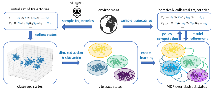
Figure 1: Overview of the algorithm CASTLE for learning MDPs modeling environments with continuous stochastic dynamics.

Step 1. - Learning an initial MDP. For the first step, CASTLE implements passive automata learning to learn an initial MDP model of the environment. This step starts from a given multiset of trajectories sampled by an existing, potentially non-optimal agent operating within the environment. For example, the trajectories could be collected during the training phase of a DRL agent. A trajectory is a sequence of observations of the environment’s state and actions chosen by the agent. This is illustrated in the top left of Fig. 1. For simple, low-dimensional, discrete applications, passive MDP learning [25] could directly be applied to learn an MDP model under the agent’s decisions from the collected trajectories of the agent. However, due to the large observation space, it is difficult for passive MDP learning to extract the relevant information and to compute a concise MDP from the original trajectories.

To overcome this issue, we (a) process the observations by performing dimensionality reduction to determine relevant information in the observations and then (b) perform clustering on the reduced observations. Finally, (c) we use the resulting clusters as equivalence classes of the original observations and apply passive automata learning over the clusters to learn a first abstraction of the MDP under the policy of the agent. These three steps are illustrated on the bottom of Fig. 1. Automata learning essentially identifies temporal dependencies between clusters and executed actions. It also splits observed clusters into different states, if they have different future behavior.

Step 2. - Fine-tuning of the model. In the second step, CASTLE iteratively improves the learned MDP model by actively gathering new information about the environment. It is likely that the initially learned model does not accurately capture the environment dynamics due to employed abstraction via dimensionality reduction and clustering. To improve the model, we actively sample new trajectories to extend our knowledge about the environment. For sampling the environment, we compute policies that solve the task under consideration from the learned intermediate models. Using the newly collected traces, we gradually increase the accuracy of learned models until the computed policies consistently solve the task. The right-hand side of Fig. 1 depicts this process.

Main contributions. To the best of our knowledge, we are the first to apply automata learning to learn models of stochastic environments over continuous state space without placing assumptions on their unknown dynamics. Having such a model makes it possible to plan ahead and to judge the agents decisions based on how likely it is that executing the agent’s actions will result in an episode that successfully completes the task. We showcase the viability of our approach by solving control tasks from OpenAI Gym [7] that serve as benchmarks for RL using policies derived from learned MDPs.

2 Related Work

Alergia [8] was an early automata learning algorithm for learning probabilistic finite automata. IoAlergia[24, 25] extends Alergia to be able to learn MDPs. Aichernig and Tappler subsequently applied IoAlergia for probabilistic verification [3]. These works have in common that observations are entirely discrete.

Instead of abstracting continuous dynamics to discrete dynamics, Niggemann et al. [31] and Medhat et al. [27] learn hybrid automata. These automata have the drawback that most analyses are undecidable. As in our approach, Kubon et al. [17] applied dimensionality reduction and passive learning to learn automata. However, they learn deterministic automata and target image classification.

Finally, there are various approaches for learning automata over infinite state spaces that place restrictive assumptions on the environment [1, 15, 35] . These works have in common that the learned automata have (uncountable) infinite state spaces, but they can express dynamics of the environment only in a limited way.

Discretization-based approaches to learning automata from cyber-physical systems have been proposed in [2, 28], but with the general drawback that the state spaces of the learned automata explode since their automata are deterministic. The problem of system identification [19, 21] addresses a similar problem, but targets hybrid systems rather than stochastic systems and places strong assumption on the properties of the identified models.

We perform a variant of model-based RL with the help of clustering. Clustering-based approaches have been proposed for the discovery of so-called options in hierarchical model-based RL [16, 23, 22] that represent subtasks of a more complex task. In contrast to us, they do not learn environmental models. In a different line of research, automata learning has been proposed to bring structure into sequences of subtasks in hierarchical RL  [36, 37, 30, 11, 13, 14]. These works infer discrete, deterministic automata, like reward machines, to enable RL with non-Markovian rewards. They serve as a high-level specification of a complex task, rather than a representation of the environment.

Hence, most related work from formal methods and AI either focuses on system verification or modeling of tasks. Both take an agent-centric view, whereas we focus on modeling the environment. Having an MDP representation of the environment makes it possible to analyze the agent’s decision making. To the best of our knowledge, there is no other automata learning approach with the same focus and capabilities with which we could compare directly.

3 Preliminaries

3.1 Markov Decision Processes

Given a finite set $S$, $Dist(S)$ denotes the set of probability distributions over $S$ and $\mathit{supp}(\mu)$ for $\mu\in Dist(S)$ denote the support of $\mu$, i.e. the set $S^{\prime}\subset S$ with $s\in S^{\prime}:\mu(s)>0$.

A Markov decision process (MDP) is a tuple $\langle\mathcal{S},s_{0},\mathcal{A},\mathcal{P}\rangle$ where $\mathcal{S}$ is a(n) (in)finite set of states, $s_{0}\in Dist(\mathcal{S})$ is a distribution over initial states, $\mathcal{A}$ is a finite set of actions, and $\mathcal{P}:\mathcal{S}\times\mathcal{A}\rightarrow\mathit{Dist}(\mathcal{S})$ is the probabilistic transition function. For all $s\in\mathcal{S}$ the available actions are $\mathcal{A}(s)=\{a\in\mathcal{A}\>|\>\exists s^{\prime},\mathcal{P}(s,a)(s^{\prime})\neq 0\}$ and we assume $|\mathcal{A}(s)|\geq 1$. The environments we consider have infinite state space.

Trajectories. A finite trajectory $\tau$ through an MDP is an alternating sequence of states and actions, i.e. $\tau=s_{0}a_{1}s_{1}\cdots a_{n-1}s_{n-1}a_{n}s_{n}\in s_{0}\times(\mathcal{A}\times\mathcal{S})^{*}$.

Policy. A policy resolves the non-deterministic choice of actions in an MDP. It is a function mapping trajectories to distributions over actions. We consider memoryless policies that take into account only the last state of a trajectory, i.e., policies $\pi:\mathcal{S}\rightarrow Dist(\mathcal{A})$. A deterministic policy $\pi$ always selects a single action, i.e., $\pi:\mathcal{S}\rightarrow\mathcal{A}$.

Deterministic labeled MDPs are defined as MDPs $\mathcal{M}_{L}=\langle\mathcal{S},s_{0},\mathcal{A},\mathcal{P},L\rangle$ with a finite set of states, and a unique initial state $s_{0}\in\mathcal{S}$, and with a labeling function $L:\mathcal{S}\rightarrow O$ mapping states to observations from a finite set $O$. The transition function $\mathcal{P}$ must satisfy the following determinism property: $\forall s\in\mathcal{S},\forall a\in\mathcal{A}:\delta(s,a)(s^{\prime})>0\land\delta(s,a)(s^{\prime\prime})>0$ implies $s^{\prime}=s^{\prime\prime}$ or $L(s^{\prime})\neq L(s^{\prime\prime})$. Given a trajectory $\tau$ in a deterministic labeled MDP $\mathcal{M}_{L}$, applying the labeling function on all states of the trajectory $\tau$ results in a so called observation trace $L(\tau)=L(s_{0})a_{1}L(s_{1})\cdots a_{n-1}L(s_{n-1})a_{n}L(s_{n})$. Note that due to determinism, an observation trace $L(\tau)$ uniquely identifies the corresponding trajectory $\tau$.

In this paper, we use passive automata learning to compute abstract MDPs of the environment under an agent’s policy in the form of deterministic labeled MDPs. The labeled MDPs capture the information required for the agent to make its decision on how to successfully complete its task.

3.2 Learning of MDPs

We learn deterministic labeled MDPs via the algorithm IOAlergia [24, 25], an adaptation of Alergia [8]. IOAlergia takes a multiset $\mathcal{T}_{o}$ of observation traces as input. In a first step, IOAlergia constructs a tree that represents the observation traces by merging common prefixes. The tree has edges labeled with actions and nodes that are labeled with observations. Each edge corresponds to a trace prefix with the label sequence that is visited by traversing the tree from the root to the node reached by the edge. Additionally, edges are associated with frequencies that denote how many traces in $\mathcal{T}_{o}$ have the trace corresponding to an edge as a prefix. Normalizing these frequencies would already yield a tree-shaped MDP.

For generalization, the tree is transformed into an MDP with cycles through iterated merging of nodes. Two nodes are merged if they are compatible, i.e., their future behavior is sufficiently similar. For this purpose, we check if the observations in the subtrees originating in the nodes are not statistically different. A parameter $\epsilon$ controls the significance level of the applied statistical tests. If a node is not compatible with any other node, it is promoted to an MDP state. Once all pairs of nodes have been checked, the final deterministic labeled MDP is created by normalizing the frequencies on the edges to yield probability distributions for the transition function $\mathcal{P}$. In this paper, we refer to this construction as MDP learning.

4 Overview of CASTLE

Figure 2: States observed in the Mountain Car environment.

Setting. We consider settings in which an agent has to perform an episodic task in an environment modeled as an MDP $\mathcal{M}=\langle\mathcal{S},s_{0},\mathcal{A},\mathcal{P}\rangle$. An episodic task is a task that has an end, i,e., ends in a terminal state of $\mathcal{M}$. An episode is a sequence of agent-environment interactions from a randomly distributed initial state of $M$ to a terminal state. An episode successfully completes the task to be learned if it ends in a (terminal) goal state. If an episode ends in a bad (terminal) state, the episode fails to complete the task.

In our setting, $\mathcal{M}$ is an MDP with continuous state space $\mathcal{S}\subseteq\mathbb{R}^{h}$ and unknown stochastic dynamics and structure. Thus, we do not assume knowledge about the reachable states or transitions of $\mathcal{M}$.

We are given a multiset of trajectories $\mathcal{T}$ sampled from $\mathcal{M}$ when executing a potentially non-optimal policy on $\mathcal{M}$. We assume that a subset of $\mathcal{T}$ are successful trajectories and end in a goal state. These trajectories serve as a starting point for passive automata learning.

Example. To illustrate the setting, consider the well-known Mountain Car environment available in OpenAI Gym [7], where the goal is to push a car up a hill. The state space of $\mathcal{M}$ consists of two real-valued variables representing the x-position of the car and its velocity. The agent has the following three actions to interact with the environment: accelerate to the left, accelerate to the right, and do nothing. In the initialization of an episode, the x-position of the car is randomly sampled from the interval $[-0.6,-0.4]$. An episode is successful if the car reaches the position $0.5$ (defines the goal terminal states in $\mathcal{M}$). After $200$ time steps (defines the terminal bad states), the episode terminates as unsuccessful. Figure 2 displays the states observed during the execution of a policy $\pi$ over $30$ episodes. Black x-markers indicate goal states at the x-position $0.5$.

Problem statement. Consider the setting as discussed above. The goal of our approach is to learn a concise model $\mathcal{M}_{a}=\langle\mathcal{S}_{a},s_{a,0},\mathcal{A},\mathcal{P}_{a},L\rangle$ in the form of an abstract deterministic labeled MDP that models the environment $\mathcal{M}$.  The model $\mathcal{M}_{a}$ should be so accurate that a policy $\pi_{a}:\mathcal{S}_{a}\rightarrow\mathcal{A}$ that solves the task to be learned in $\mathcal{M}_{a}$, also successfully solves the task when being executed on $\mathcal{M}$.

Overview of the learning process. Our approach consists of two phases: an initialization and a fine-tuning phase. The initialization phase prepares the trajectories in the continuous state space so that they can be used to learn an abstract, concise MDP model $\mathcal{M}_{a}$. Fine-tuning computes a policy based on $\mathcal{M}_{a}$ and uses it to collect additional trajectories to fine-tune $\mathcal{M}_{a}$ with more information about the environment $\mathcal{M}$. The policy $\pi_{a}:\mathcal{S}_{a}\rightarrow\mathcal{A}$ for $\mathcal{M}_{a}$ is automatically computed by solving a reachability objective through probabilistic model checking. The computed policy $\pi_{a}$ selects actions that have the maximal probability of successfully completing the task.

5 Initial Model Learning

The section covers the initialization phase of CASTLE that sets up automata learning and learns a first MDP. For the remainder of this section, let $\mathcal{M}=\langle\mathcal{S},s_{0},\mathcal{A},\mathcal{P}\rangle$, be the MDP underlying the environment with state space $\mathcal{S}\subseteq\mathbb{R}^{h}$, where $h$ is the size of the state vectors, and let $\mathcal{T}$ be a multiset of trajectories $(\mathcal{S}\times\mathcal{A})^{*}\times\mathcal{S}$. Our goal is to learn an abstract deterministic labeled MDP $\mathcal{M}_{a}$ serving as an initial model of $\mathcal{M}$ from the trajectories $\mathcal{T}$.

First, our approach transforms the trajectories in $\mathcal{T}$, which are sequences of real-valued states and actions, into observation traces, which are sequences of abstract observations and actions. The transformation consists of the steps: (1) dimensionality reduction and scaling, (2) clustering, and (3) additional labeling of states. After performing these data-processing steps, we compute an initial model $\mathcal{M}_{a}=\langle\mathcal{S}_{a},s_{a,0},\mathcal{A},\mathcal{P}_{a},L\rangle$ using IoAlergia as a final fourth step. In the following, we discuss the individual steps in detail.

1. Dimensionality Reduction and Scaling. For high-dimensional state spaces, we apply a dimensionality reduction $sd:\mathcal{S}\rightarrow\mathcal{S}^{d}$ to transform $\mathcal{S}\subseteq\mathbb{R}^{h}$ to $\mathcal{S}^{d}\subseteq\mathbb{R}^{d}$ with $h>d$. We denote with $\mathcal{S}_{T}$ and $\mathcal{S}^{d}_{T}$ the set of all states and reduced states contained in $\mathcal{T}$.

While any standard technique like principle component analysis [26] can be applied, we propose to apply a dimensionality reduction approach that works with the given trajectories in $\mathcal{T}$ instead of working only with the observed states. Thus, we propose to guide the selection of the dimensionality reduction by the actions taken in the observed states. For control applications, the information loss incurred by dimensionality reduction is low, if the action taken in a state can be predicted with the same accuracy in $\mathbb{R}^{d}$ as in $\mathbb{R}^{h}$.

Linear discriminant analysis (LDA) is a natural fit for classifying states according to actions fully automatically. LDA can be applied to compute discriminant functions mapping states to actions such that they match the state-action pairs of the demonstration trajectories. That is, we apply LDA to learn a classifier from states to actions using the demonstrations $\mathcal{T}$. This enables reducing the dimensionality by projection to the $d$ most discriminative axes.

Alternatively, we propose a semi-manual technique for dimensionality reduction using decision trees (DTs). If domain knowledge is available, it can be used to extract $d$ features from the states and train DTs with a bounded size to classify states to actions. If the classification accuracy of DTs trained in $\mathbb{R}^{d}$ (reduced states) is similar to the accuracy in $\mathbb{R}^{h}$ (original states), we assume that the $d$ extracted features are sufficient for the task at hand. The choice of the $d$ features allows a dimensionality reduction with a small loss of information.

Note that dimensionality reduction is optional and can be skipped if the number of dimensions is low. After dimensionality reduction, the reduced states can be further prepared for ideal clustering by applying power transformation [38] and scaling the state data to zero mean and unit variance.

2. Clustering. In the next step, CASTLE applies a clustering function $\mathit{clust}:\mathcal{S}^{d}\rightarrow K$ to assign cluster labels $K=\{1,\dots,k\}$ to dimensionality-reduced states. To facilitate an application in CASTLE, the clustering approach should enable estimating cluster membership via distances, and it should be efficient. CASTLE exploits the first property to simulate learned MDPs during sampling; see Section 6. One clustering approach that satisfies these requirements is the popular $k$-means algorithm [20].

3. Labeling. In the next step, CASTLE assigns a set of labels to the states in a trajectory in reduced dimensions. The labels are observations that are crucial for computing a policy over a learned MDP.

We define a labeling function $\mathit{lab}:\mathcal{S}^{d}\times\mathbb{N}_{0}\rightarrow 2^{O}$, for a set of observations $O=\{\mathit{init},\mathit{goal},\mathit{bad}\}\,\cup\,K$. The function assigns labels to $(s,i)$ where $s$ is a state at index $i$ in a trajectory. A pair $(s,i)$ is labeled with $\mathit{init}$, if $i=0$, i.e., $s$ is an initial state in a demonstration trajectory. For any other $(s,i)$, the cluster label $\mathit{clust}(s)$ is contained in $\mathit{lab}(s,i)$. Furthermore, we have $\mathit{goal}\in\mathit{lab}(s,i)$ if $s$ is a goal state or $\mathit{bad}\in\mathit{lab}(s,i)$ if $s$ is a bad state. Both depend on $i$, since tasks may define a time limit for successful completion. If additional domain knowledge is available, it can be used to assign additional labels to states, e.g., to indicate potentially dangerous situations.

4. MDP Learning. To learn an MDP from trajectories $\mathcal{T}$, CASTLE transforms the trajectories into observation traces $\mathcal{T}_{O}$, by sequentially applying dimensionality reduction, scaling, clustering, and labeling. Given $\mathcal{T}_{O}$ as input, IoAlergia computes a deterministic labeled MDP $\mathcal{M}_{a}$, which provides an abstract representation of the environment dynamics. The introduction of the $\mathit{init}$ label for initial states enables modeling environments where the initial states are randomly distributed. Introducing the $\mathit{init}$ observation basically ignores the concrete initial environment states. Consequently, the transitions from the learned initial state (labeled $\mathit{init}$) include the distribution of initial environment states.

Example. The colors in Fig. 2 indicate different clusters of states derived with k-means and k=16 and the black x-markers indicate goal states. Thus, the states on the right-hand side of the figure have two labels corresponding to the clusters and the label $\mathit{goal}$. All other states have a single label corresponding to a cluster unless they are reached at the end of an episode, in which case they are labeled $\mathit{bad}$ to indicate a timeout. Thus, states that are observed at different times may be labeled differently when abstracting a trajectory to an observation trace. An example of an observation trace may be $\{\mathit{init}\}\cdot\mathit{left}\cdot\{c_{1}\}\cdot\mathit{right}\cdot\{c_{1}\}\cdots\mathit{right}\cdot\{c_{15},\mathit{goal}\}$. It starts with $\mathit{init}$ and then alternates between actions and observations that include cluster labels. The final observation includes $\mathit{goal}$ to indicate a successful episode. With this information, IoAlergia is able to learn temporal dependencies between observations and actions.

6 Model Fine-Tuning

The fine-tuning phase of CASTLE incrementally improves the learned labeled MDP $\mathcal{M}_{a}$ that models the environment $\mathcal{M}$. In a nutshell, the fine-tuning phase iteratively (1) computes a policy that is able to solve the task in $\mathcal{M}_{a}$ via probabilistic model checking, (2) uses the policy to sample new trajectories, and (3) learns a new, improved model with the extended multiset of trajectories.

The fine-tuning phase is based on the approach proposed by Aichernig and Tappler [3]. In contrast to the original approach, which works solely on abstract observations, our fine-tuning approach takes the concrete state space and the uncertainties stemming from clustering into account. In the following, we discuss the individual steps of our fine-tuning approach in detail.

1. Policy Computation. Given $\mathcal{M}_{a}=\langle\mathcal{S}_{a},s_{a,0},\mathcal{A},\mathcal{P}_{a},L\rangle$, our goal is to compute a (deterministic) policy $\pi_{a}:\mathcal{S}_{a}\rightarrow\mathcal{A}$ that maximizes the probability to complete the task successfully, i.e., reaching a goal state in $\mathcal{M}_{a}$. Thus, for any state $s_{a}\in\mathcal{S}_{a}$, the policy $\pi_{a}$ picks the action $a_{\pi}=\pi_{a}(s_{a})$ that maximizes the probability of reaching a goal state. Such policies can be automatically computed via probabilistic model checking (using tools like Prism [18]). Let $p_{s,a}=P_{\mathrm{max}}(\mathbf{F}\ \mathit{goal},s_{a},a)$ be the maximal probability of reaching a goal state from state $s_{a}$ when executing action $a$, where $\mathbf{F}$ denotes the eventually operator. For any state $s_{a}\in\mathcal{S}_{a}$, we have $a_{\pi}=\pi(s_{a})$ with $a_{\pi}=\max_{a\in\mathcal{A}}p_{s_{a},a}$.

2. Sampling. In the next step of the iterative model refinement phase, CASTLE uses the policy $\pi_{a}:\mathcal{S}_{a}\rightarrow\mathcal{A}$ over the current $\mathcal{M}_{a}$ to sample additional trajectories in $\mathcal{M}$. The newly sampled trajectories are added to the existing trajectories $\mathcal{T}$ and are used in the next step to improve the accuracy of $\mathcal{M}_{a}$.

Overview of sampling of trajectories. For the sampling, the learned MDP $\mathcal{M}_{a}=\langle\mathcal{S}_{a},s_{a,0},\mathcal{A},\mathcal{P}_{a},L\rangle$ is simulated in parallel with the environment $\mathcal{M}=\langle\mathcal{S},s_{0},\mathcal{A},\mathcal{P}\rangle$. The actions are selected via the policy $\pi_{a}:\mathcal{S}_{a}\rightarrow\mathcal{A}$, computed in the previous step.

During sampling, the MDP $\mathcal{M}_{a}$ is treated similarly to a partially observable MDP (POMDP). To account for inaccuracies in $\mathcal{M}_{a}$, we adopt the notion of belief states (belief for short). A belief $B$ is a distribution over the states $\mathcal{S}_{a}$, i.e., at any time step of the current episode, the $\mathcal{M}_{a}$ is in state $s_{a}\in\mathcal{S}_{a}$ with probability $B(s_{a})$. The belief update is both based on the structure of learned MDP $\mathcal{M}_{a}$ as well as the environment state reached after a step. In time step $i$, after having taken an action $act$ and the environment having moved to a state $s^{\prime}\in\mathcal{S}$ in cluster $k^{\prime}$, we update the belief $B$ to $B^{\prime}$ to include states $s_{a}^{\prime}$ with $\mathcal{P}_{a}(s_{a},act,s_{a}^{\prime})>0$ for $s_{a}\in\mathit{supp}{B}$. That is, we move to states reachable in $\mathcal{M}_{a}$. The probabilities $B^{\prime}(s_{a}^{\prime})$ are the product of $B(s_{a})$, i.e., the previous state probability, and a term that is inversely proportional to the distance between the cluster centroid of $k^{\prime}$ (the reached cluster) and the centroid of the cluster in $L(s_{a}^{\prime})$.

Consider the following scenario to see why keeping track of a single state $s_{a}\in\mathcal{S}_{a}$ is not sufficient. Suppose that in the current episode, the environment $\mathcal{M}$ is in a state $s\in\mathcal{S}$ and the learned model $\mathcal{M}_{a}$ is in a state $s_{a}\in\mathcal{S}_{a}$. In the next time step, the environment moves from state $s$ to $s^{\prime}$ via action $act$. The corresponding cluster labels of the states $s$ and $s^{\prime}$ are $k$ and $k^{\prime}$, respectively. Ideally, in the learned model $\mathcal{M}_{a}$, there is a unique $s^{\prime}_{a}$ corresponding to $s^{\prime}$ identified by $\mathcal{P}_{a}(s_{a},a,s_{a}^{\prime})>0$ with $k^{\prime}\in L(s_{a}^{\prime})$. However, since the learned models are not perfectly accurate, especially during early iterations, this is not always the case.

Algorithm 1 Sampling with a policy computed from a learned MDP.

1:$\mathcal{M}=\langle\mathcal{S},s_{0},\mathcal{A},\mathcal{P}\rangle$, model $\mathcal{M}_{a}=\langle\mathcal{S}_{a},s_{a,0},\mathcal{A},\mathcal{P}_{a},L\rangle$, policy $\pi:\mathcal{S}_{a}\rightarrow\mathcal{A}$, clusters $K$, max. belief size $b_{n}$

2:A sampled trajectory $\tau$

3:$s\in\mathcal{S}\leftarrow\texttt{reset()}$

4:$\tau\leftarrow s$

5:$B\leftarrow\{s_{a,0}\mapsto 1\}$

6:while $s$ is not terminal do

7:    $ba\leftarrow\{a\mapsto\sum_{s_{a}\in\mathcal{S}_{a},\pi_{a}(s_{a})=act}B(s_{a})|act\in\mathcal{A}\}$

8:    sample $act\sim ba$

9:    $s\leftarrow\texttt{step}(act)$

10:    $\tau\leftarrow\tau\cdot act\cdot s$

11:    $dists\leftarrow\{k\mapsto dist(sd(s),centroid(k))|k\in K\}$

12:    $cDistr\leftarrow\textit{cdf. of }\mathcal{N}(mean(dists);stddev(dists)^{2})$

13:    $B^{\prime}\leftarrow\{s_{a}\mapsto 0|s_{a}\in\mathcal{S}_{a}\}$

14:    for $s_{a}\in\mathit{supp}(B)$, $s_{a}^{\prime}\in\mathit{supp}(\mathcal{P}_{a}(s_{a},act))$ do

15:        $k^{\prime}\leftarrow L(s_{a}^{\prime})\cap K$

16:        $B^{\prime}(s_{a}^{\prime})\leftarrow B^{\prime}(s_{a}^{\prime})+B(s_{a})\cdot(1-cDistr(k^{\prime}))$     

17:    $B^{\prime}\leftarrow\{s_{a}\mapsto p\in B^{\prime}|p\textit{ is in the }b_{n}\textit{ largest values of }B^{\prime}(\cdot)\}$

18:    $B^{\prime}\leftarrow\{s_{a}\mapsto\frac{p}{\sum_{s_{a}^{\prime}}B(s_{a}^{\prime})}|s_{a}\mapsto p\in B^{\prime}\}$

19:return $\tau$

Algorithm for sampling of trajectories. Algorithm 1 formalizes our approach to sample a trajectory from $\mathcal{M}$ using a policy computed from a learned model $\mathcal{M}_{a}$. We follow the OpenAI Gym [7] conventions and use the operations reset and step to change the current state $s$ of the environment $\mathcal{M}$. The function reset resets $\mathcal{M}$ to an initial state and returns this state. The function step takes an action $a$ as input, executes $a$, and returns the reached state $s^{\prime}$.

In Algo. 1, the Lines 3 to 5 perform initialization steps by resetting the environment, adding the initial state to the sampled trajectory $\tau$, and initializing the belief $B$ to include only the initial state of $\mathcal{M}_{a}$.

We then sample experiences from $\mathcal{M}$ until reaching a terminal state (Line 6). Line 7 transforms the belief state into a distribution over actions by mapping states to actions chosen by the policy $\pi_{a}$. The next $3$ lines sample an action, execute it in the environment, and append the new state-action pair to the trajectory $\tau$. Hence, the combination of the current belief and a deterministic policy $\pi_{a}$ yields a probabilistic policy.

Starting in Line 11, we begin the update of the belief state. First, we compute the Euclidean distances from all cluster centroids to the current environment state in reduced dimensions. We then fit a normal distribution over distances, which we empirically found to be a good fit. After that, we initialize the next belief state $B^{\prime}$ and iterate over all states reachable in $\mathcal{M}_{a}$ (Line 14). In Line 16, we add the contribution of $s_{a}^{\prime}$ to the next belief $B^{\prime}$ as the product of the previous belief $B(s_{a})$ and the inverse of the distance probability of the cluster $k^{\prime}$ labeling $s_{a}^{\prime}$. We use the inverse to favor short distances and to ignore $\mathcal{P}(s_{a},a)$ so that we only consider the actual environment information for the belief update. In Line 17 we discard states with low probability. Finally, Line 18 normalizes the belief to a distribution.

3. Learning and Stopping. In each iteration of the fine-tuning phase, we sample $n_{\mathrm{samples}}$ additional trajectories from $\mathcal{M}$, as outlined above. To learn a more accurate model $\mathcal{M}_{a}$ from the additional information, CASTLE takes the newly collected trajectories $\mathcal{T}^{new}$ and transforms them into observation traces $\mathcal{T}^{new}_{O}$. This is done by sequentially applying dimensionality reduction, scaling, clustering, and labeling as outlined in Sect. 5. CASTLE adds the new observation traces to the existing multiset of traces $\mathcal{T}_{O}$ and learns a labeled MDP $\mathcal{M}_{a}$ with IoAlergia. After computing a new learned model $\mathcal{M}_{a}$, CASTLE returns to the policy computation step.

As stopping criteria for the iteration, one can stop either after a fixed number of iterations or upon reaching a goal state a specified number of times in the current iteration.

7 Experiments

Environment	Demonstration Trajectories	Demonstration Timesteps	Dimensionality Reduction	Clusters	Fine-tuning Iterations	Episodes Per Fine-tuning	Final Model Size	Best Policy Reward	Goal Reached
Acrobot	2500	2.1 $\times 10^{5}$	Manual Mapper LDA + Power Transformer	256	25	50	472 482	-113 $\pm$ 41 -156 $\pm$ 63	42% | 82% 4% | 35%
Lunar Lander	2500	5.6 $\times 10^{5}$	Manual Mapper LDA + Power Transformer	512	25	50	1122 1100	213 $\pm$ 80 103 $\pm$ 138	81% 35%
Mountain Car	2500	3 $\times 10^{5}$	Power Transformer	256	25	50	363	-136 $\pm$ 28	42%
Cartpole	2500	5 $\times 10^{5}$	Power Transformer	128	15	50	213	195 $\pm$ 18	88%

Table 1: Parameterized results for all environments. All values are averages from five experiment runs.

We applied CASTLE to four well-known RL applications [7]: (1) Acrobot, (2) Lunar Lander, (3) Mountain Car, and (4) Cartpole. All reported results are average values over five experiment runs per environment. Pretrained Stable-Baselines3 [32] RL agents that achieved high reward on their respective tasks were downloaded from HuggingFace. Model learning was done with AALpy [29]. For the computation of the policies over the learned models we used the model checker Prism [18]. All experiments were conducted on a laptop with an Intel^® Core™i7-11800H CPU at 2.3 GHz with 32 GB of RAM. Source code and detailed instructions to reproduce our experiments are available in the supplementary material.

Results. Table 1 contains the parameterized results for each experiment. The “Demonstration Trajectories” column gives the total number of episodes/trajectories, which we sampled using a DRL agent downloaded from the https://huggingface.co/ library. The column “Demonstration Timesteps” lists the timesteps performed on the environment during the sampling of demonstrations, i.e., the combined length of the demonstration trajectories.

Please note the compact size of the learned models in the column “Final Model Size”. In all experiments, each environment state was observed only once (due to the continuous state space). The total number of observed states is thus equal to the number of timesteps. Therefore, if we would directly apply automata learning, the learned MDP would have [2.1-5.6]$\times 10^{5}$ states. The learned MDPs of CASTLE have [213-1122] states. Next, we discuss the results of the individual experiments in more detail.

(a) Acrobot

(b) Lunar Lander

(c) Mountain Car

(d) Cartpole

Figure 3: Mean and standard deviation of all experiments over multiple fine-tuning iterations

Acrobot. Acrobot is a two-link pendulum that is actuated by a single joint. Its state space consists of $6$-dimensional real-valued vectors encoding link angles and angular velocities. The goal is to swing the bottom link of the pendulum up to a target height in as few steps as possible. The task is considered to be solved, if the target can be achieved in 100 steps, shown as a green line in Fig. 3(a). We evaluated our method with two different dimensionality reduction techniques: using a manually created dimensionality reduction via decision trees and using LDA. As seen in Tab. 1, both approaches can find a model which allows to solve the task in 42% and 4% of cases. These results are still remarkable given that our approach computes a control policy to merely maximize the probability of solving the task, but does not necessarily optimize for maximum rewards like RL agents. If we reduce the goal from 100 steps to 130 steps, we observe that our models can compute a policy that reaches this goal in 82% and 35% of cases. Fig. 3(a) shows the averaged gained rewards throughout learning. The red line indicates the average reward gained with manual dimensionality reduction and the red-shaded area shows the standard deviation of the gained area. The results for LDA-based dimensionality reduction are shown in blue. We can observe that the models with manual dimensionality reduction yield to a good policy after just 4 iterations of fine-tuning (total of 200 episodes). LDA-based dimensionality reduction leads to policies achieving less stable, but still high rewards.

Lunar Lander. Lunar lander is a classic rocket trajectory optimization problem. The task is to land the rocket in the landing area as fast as possible. At the beginning of each episode, a random force is applied to the rocket. Its state space consists of $8$-dim. vectors. We compared our learned models for two different dim. reductions with three DRL agents trained via stable-baselines . All stable-baselines agents are able to land the rocket successfully. As shown in Fig. 3(b), the learned models are accurate enough after only 8 fine-tuning iterations to allow the computation of a good policy. The graphs follow the same color coding as for Acrobot, with the exception that the DRL agent results are shown with markers. We observe a performance gap between models computed from the manually-crafted dim. reduction and the LDA-based one. As seen in Table 1, the policy constructed with manually-created dim. reduction successfully lands with a probability of 81%, compared to 35% of the LDA-based policy. However, the policies for both models are safe and do not crash the rocket. Through visual inspection, we found that if our policy does not land successfully, it hovers close to the landing position. It is noteworthy that the policy computed with manual dim. reduction even outperforms two of the DRL agents and gets close to the third agent that was trained using PPO [33].

Mountain Car. Mountain car is a control problem, where an agent needs to bring a car to the top of a steep hill in less than 200 steps. Environmental states consist of 2 real values, the x-position of the car and its velocity, therefore we perform no dimensionality reduction. As policies computed from our learned models easily complete this task, we compare to the mean reward of the agent we used to sample demonstration trajectories. This reference is shown as a green line in Fig. 3(c). The dashed and dotted lines depict the mean reward gained when learning a model over $k=128$ and $k=64$ clusters, respectively. The red line and red-shaded area show the mean and standard deviation of the reward gained with $256$ clusters. In this configuration, our approach with 256 clusters computed an MDP with 363 states that leads to a slightly less performant policy than the RL agent (-136$\pm$ 28 compared to -110$\pm$19). These results indicate that our method successfully learns close-to-optimal policies, even considering that it does not necessarily optimize for rewards, but towards a reachability objective. We further observe that a larger value for $k$ leads to a better policy. This can be attributed to the fact that a larger number of clusters helps to differentiate states during MDP learning.

Cartpole. Cartpole is a classic control problem in which an agent needs to balance a pole attached to a cart. The task is considered solved with a reward of 195 [6], that is, the pole is balanced for at least 195 steps. This translate to a reward of $195$ shown as a green line in Fig. 3(d). Its states are encoded as 4-dimensional real-valued vectors. As seen in Tab. 1, our approach solved the game in 15 fine-tuning iterations (750 episodes) with a 213-state MDP, achieving an average reward of 195$\pm$18. Like for Mountain Car, we show the mean and standard deviation for one configuration ($k=128$) in red and for two lower settings of $k$, we show the mean reward. We again see that a larger $k$ leads to better performance.

Hyperparameter selection. To select the appropriate number of clusters $k$ in k-means, we have applied the elbow method as a starting heuristic. We observed that, for the considered environments, after 128 clusters the k-means inertia decreases. However, after further experimentation, we observed that a higher number of clusters correlates with increased performance of the model but with higher computational costs, especially in the MDP learning. Therefore, we consider the perceived complexity of the environment to select a concrete $k$. Since we aim for very few assumptions on the environment, we used the number of dimensions of the original state space of each environment as a complexity estimate.

The number of demonstration trajectories was set to 2500 for all experiments. This value was selected to ensure enough data points to compute sufficiently accurate dimensionality reduction and clustering accuracy. The number is further motivated by the number of training timesteps of one of the DRL agents we use for comparison. The Mountain Car A2C agent was trained for $10^{6}$ time steps, which requires at least $5000$ episodes, as the maximum episode length is $200$. Hence, we decided on using half of that for the initialization phase of our approach. The number of fine-tuning iterations, which we set to $25$, and episodes per iteration $n_{samples}=50$ was selected so that the total number of sampled trajectories is half of the demonstration trajectories. This setting ensures relatively low sampling compared to RL agents, while the results indicate that the fine-tuning of the model can converge to a close-to-optimal solution in a few iterations.

IOAlergia’s $\epsilon$ parameterwas set to $0.005$ for all experiments. We experimented with other values, with minimal impact on model quality. As pointed by [9]: "The algorithm behaved robustly with respect to the choice of parameter epsilon".

Furthermore, we observed that our approach is robust w.r.t. the maximal belief size, therefore we set $b_{n}=4$ for all experiments.

Discussion. Our experiments show that CASTLE learns deterministic labeled MDPs with sufficient fidelity to compute policies that solve control tasks in their respective environments. The approach has a sample complexity comparable to DRL. For each task, we have sampled $2500$ trajectories, plus additional $1250$ trajectories per refinement iteration. For example, let’s analyze the number of time steps for the Mountain Car experiment. We sample the environment for approx. $3\times 10^{5}$ time steps to sample the initial trajectories, plus additional $1.9\times 10^{5}$ steps for the fine-tuning, which is $=4.9\times 10^{5}$ time steps in total. This is less then the sampling performed for the A2C agent that we use for comparison, which was trained for $10^{6}$ time steps. In its current form, the runtime of CASTLE is slightly higher than of DRL due to the absence of GPU-accelerated computation. On average, a single experiment for each of the case studies took between 60 and 90 minutes, but this runtime could be improved.

While policies computed via CASTLE solved all tasks, they often achieved lower reward than DRL agents. This was to be expected since our learned models do not consider rewards and only optimize for successfully solving the task. We leave including rewards in the learned models to future work. However, please note that the main goal of learning a compact environmental model is not to beat the performance of advanced deep RL agents. Rather, having a compact environmental model offers many possibilities to evaluate and to explain the decision-making of DRL agents.

8 Conclusion

We proposed an automata learning approach for learning discrete, abstract MDP models of environments with continuous state space and unknown stochastic dynamics. The learning is split into two phases, a passive and an active phase. In the first phase, we learn an initial model from a given set of sampled trajectories. To prepare the data for learning, we compute a state abstraction by applying dimensionality reduction, clustering, and labeling of states. In the second phase, we incrementally improve the accuracy of the learned model by actively sampling additional trajectories and use them for learning a new model. For sampling, we compute policies that maximize the probability of solving the task in the learned model via probabilistic model checking. We showcase the potential of our approach by solving popular control problems available in OpenAI gym [7]. In some instances, the computed policies of the learned model achieve even higher rewards than DRL agents although we do not explicitly optimize for rewards.

We see several promising avenues for future work. First, we want to use CASTLE to evaluate trained RL agents for challenging application domains. The learned models can be used to analyze the agent’s decision-making in crucial states. Furthermore, in case we detect incorrect behavior, we want to study how we can use the models to explain the detected issue and to guide the retraining of an agent to repair its policy. Another interesting line of research would be to use the learned models as runtime monitors to detect potentially unsafe behavior of the agent during execution. Furthermore, we want to study whether the computed policies over the learned models can be used to enforce safety during runtime (aka shielding [4]). Finally, we see several possible algorithmic extensions. For example, we want to enhance the learned MDPs with rewards to improve the rewards gained by the computed policies.

Acknowledgments.

This work has been supported by the "University SAL Labs" initiative of Silicon Austria Labs (SAL) and its Austrian partner universities for applied fundamental research for electronic based systems. This work also received funding from the State Government of Styria, Austria – Department Zukunftfonds Steiermark.

References

- [1] Fides Aarts, Faranak Heidarian, Harco Kuppens, Petur Olsen, and Frits W. Vaandrager, ‘Automata learning through counterexample guided abstraction refinement’, in FM 2012, volume 7436, pp. 10–27. Springer, (2012).
- [2] Bernhard K. Aichernig, Roderick Bloem, Masoud Ebrahimi, Martin Horn, Franz Pernkopf, Wolfgang Roth, Astrid Rupp, Martin Tappler, and Markus Tranninger, ‘Learning a behavior model of hybrid systems through combining model-based testing and machine learning’, in ICTSS 2019, volume 11812, pp. 3–21. Springer, (2019).
- [3] Bernhard K. Aichernig and Martin Tappler, ‘Probabilistic black-box reachability checking’, in RV 2017, volume 10548, pp. 50–67. Springer, (2017).
- [4] Mohammed Alshiekh, Roderick Bloem, Rüdiger Ehlers, Bettina Könighofer, Scott Niekum, and Ufuk Topcu, ‘Safe reinforcement learning via shielding’, in Conference on Artificial Intelligence (AAAI-18) 2-7, 2018, eds., Sheila A. McIlraith and Kilian Q. Weinberger, pp. 2669–2678, (2018).
- [5] Christel Baier, Luca de Alfaro, Vojtěch Forejt, and Marta Kwiatkowska, Model Checking Probabilistic Systems, 963–999, Springer International Publishing, Cham, 2018.
- [6] Andrew G. Barto, Richard S. Sutton, and Charles W. Anderson, ‘Neuronlike adaptive elements that can solve difficult learning control problems’, IEEE Trans. Syst. Man Cybern., 13(5), 834–846, (1983).
- [7] Greg Brockman, Vicki Cheung, Ludwig Pettersson, Jonas Schneider, John Schulman, Jie Tang, and Wojciech Zaremba, ‘OpenAI gym’, CoRR, abs/1606.01540, (2016).
- [8] Rafael C. Carrasco and José Oncina, ‘Learning stochastic regular grammars by means of a state merging method’, in ICGI 1994, volume 862, pp. 139–152. Springer, (1994).
- [9] Rafael C. Carrasco and José Oncina, ‘Learning deterministic regular grammars from stochastic samples in polynomial time’, RAIRO Theor. Informatics Appl., 33(1), 1–20, (1999).
- [10] Joeri de Ruiter and Erik Poll, ‘Protocol state fuzzing of TLS implementations’, in USENIX Security 15, 2015, pp. 193–206. USENIX Association, (2015).
- [11] Taylor Dohmen, Noah Topper, George K. Atia, Andre Beckus, Ashutosh Trivedi, and Alvaro Velasquez, ‘Inferring probabilistic reward machines from non-markovian reward signals for reinforcement learning’, in ICAPS 2022, pp. 574–582. AAAI Press, (2022).
- [12] Paul Fiterau-Brostean, Ramon Janssen, and Frits W. Vaandrager, ‘Combining model learning and model checking to analyze TCP implementations’, in CAV 2016, Part II, volume 9780, pp. 454–471. Springer, (2016).
- [13] Daniel Furelos-Blanco, Mark Law, Alessandra Russo, Krysia Broda, and Anders Jonsson, ‘Induction of subgoal automata for reinforcement learning’, in AAAI 2020, (2020).
- [14] Maor Gaon and Ronen I. Brafman, ‘Reinforcement learning with non-markovian rewards’, in AAAI 2020, pp. 3980–3987. AAAI Press, (2020).
- [15] Olga Grinchtein, Bengt Jonsson, and Martin Leucker, ‘Learning of event-recording automata’, in FORMATS 2004 and FTRTFT 2004, volume 3253, pp. 379–396. Springer, (2004).
- [16] Ramnandan Krishnamurthy, Aravind S. Lakshminarayanan, Peeyush Kumar, and Balaraman Ravindran, ‘Hierarchical reinforcement learning using spatio-temporal abstractions and deep neural networks’, CoRR, abs/1605.05359, (2016).
- [17] David Kubon, Frantisek Mráz, and Ivan Rychtera, ‘Learning automata using dimensional reduction’, in IBERAMIA 2022, volume 13788, pp. 41–52. Springer, (2022).
- [18] M. Kwiatkowska, G. Norman, and D. Parker, ‘PRISM 4.0: Verification of probabilistic real-time systems’, in CAV 2011, volume 6806, pp. 585–591. Springer, (2011).
- [19] Lennart Ljung, System Identification: Theory for the User, PTR Prentice Hall Information and System Sciences Series, Prentice Hall, New Jersey, 1999.
- [20] Stuart P. Lloyd, ‘Least squares quantization in PCM’, IEEE Trans. Inf. Theory, 28(2), 129–136, (1982).
- [21] Chen Lv, Yahui Liu, Xiaosong Hu, Hongyan Guo, Dongpu Cao, and Fei-Yue Wang, ‘Simultaneous observation of hybrid states for cyber-physical systems: A case study of electric vehicle powertrain’, IEEE Trans. Cybern., 48(8), 2357–2367, (2018).
- [22] Marlos C. Machado, Marc G. Bellemare, and Michael H. Bowling, ‘A laplacian framework for option discovery in reinforcement learning’, in ICML 2017, volume 70, pp. 2295–2304. PMLR, (2017).
- [23] Shie Mannor, Ishai Menache, Amit Hoze, and Uri Klein, ‘Dynamic abstraction in reinforcement learning via clustering’, in ICML 2004, volume 69. ACM, (2004).
- [24] Hua Mao, Yingke Chen, Manfred Jaeger, Thomas D. Nielsen, Kim G. Larsen, and Brian Nielsen, ‘Learning markov decision processes for model checking’, in QFM 2012, volume 103, pp. 49–63, (2012).
- [25] Hua Mao, Yingke Chen, Manfred Jaeger, Thomas D. Nielsen, Kim G. Larsen, and Brian Nielsen, ‘Learning deterministic probabilistic automata from a model checking perspective’, Machine Learning, 105(2), 255–299, (2016).
- [26] Andrzej Maćkiewicz and Waldemar Ratajczak, ‘Principal components analysis (pca)’, Computers & Geosciences, 19(3), 303–342, (1993).
- [27] Ramy Medhat, S. Ramesh, Borzoo Bonakdarpour, and Sebastian Fischmeister, ‘A framework for mining hybrid automata from input/output traces’, in EMSOFT 2015, pp. 177–186. IEEE, (2015).
- [28] Karl Meinke, ‘Learning-based testing of cyber-physical systems-of-systems: A platooning study’, in EPEW 2017, volume 10497, pp. 135–151. Springer, (2017).
- [29] Edi Muškardin, Bernhard K. Aichernig, Ingo Pill, Andrea Pferscher, and Martin Tappler, ‘Aalpy: an active automata learning library’, Innov. Syst. Softw. Eng., 18(3), 417–426, (2022).
- [30] Daniel Neider, Jean-Raphaël Gaglione, Ivan Gavran, Ufuk Topcu, Bo Wu, and Zhe Xu, ‘Advice-guided reinforcement learning in a non-markovian environment’, in AAAI 2021, pp. 9073–9080. AAAI Press, (2021).
- [31] Oliver Niggemann, Benno Stein, Asmir Vodencarevic, Alexander Maier, and Hans Kleine Büning, ‘Learning behavior models for hybrid timed systems’, in AAAI 2012. AAAI Press, (2012).
- [32] Antonin Raffin, Ashley Hill, Adam Gleave, Anssi Kanervisto, Maximilian Ernestus, and Noah Dormann, ‘Stable-baselines3: Reliable reinforcement learning implementations’, Journal of Machine Learning Research, 22(268), 1–8, (2021).
- [33] John Schulman, Filip Wolski, Prafulla Dhariwal, Alec Radford, and Oleg Klimov, ‘Proximal policy optimization algorithms’, CoRR, abs/1707.06347, (2017).
- [34] Martin Tappler, Bernhard K. Aichernig, and Roderick Bloem, ‘Model-based testing IoT communication via active automata learning’, in ICST 2017, pp. 276–287. IEEE Computer Society, (2017).
- [35] Sicco Verwer, Mathijs de Weerdt, and Cees Witteveen, ‘A likelihood-ratio test for identifying probabilistic deterministic real-time automata from positive data’, in ICGI 2010, volume 6339, pp. 203–216. Springer, (2010).
- [36] Zhe Xu, Ivan Gavran, Yousef Ahmad, Rupak Majumdar, Daniel Neider, Ufuk Topcu, and Bo Wu, ‘Joint inference of reward machines and policies for reinforcement learning’, in ICAPS, (2020).
- [37] Zhe Xu, Bo Wu, Aditya Ojha, Daniel Neider, and Ufuk Topcu, ‘Active finite reward automaton inference and reinforcement learning using queries and counterexamples’, in CD-MAKE, (2021).
- [38] In-Kwon Yeo and Richard A. Johnson, ‘A new family of power transformations to improve normality or symmetry’, Biometrika, 87(4), 954–959, (12 2000).