Broken-symmetry magnetic phases in two-dimensional triangulene crystals

Abstract

We provide a comprehensive theory of magnetic phases in two-dimensional triangulene crystals, using both Hubbard model and density functional theory (DFT) calculations. We consider centrosymmetric and non-centrosymmetric triangulene crystals. In all cases, DFT and mean-field Hubbard model predict the emergence of broken-symmetry antiferromagnetic (ferrimagnetic) phases for the centrosymmetric (non-centrosymmetric) crystals. This includes the special case of the [4,4]triangulene crystal, whose non-interacting energy bands feature a gap with flat valence and conduction bands. We show how the lack of contrast between the local density of states of these bands, recently measured via scanning tunneling spectroscopy, is a natural consequence of a broken-symmetry Néel state that blocks intermolecular hybridization. Using random phase approximation, we also compute the spin wave spectrum of these crystals, including the recently synthesized [4,4]triangulene crystal. The results are in excellent agreement with the predictions of a Heisenberg spin model derived from multi-configuration calculations for the unit cell. We conclude that experimental results are compatible with an antiferromagnetically ordered phase where each triangulene retains the spin predicted for the isolated species.

I Introduction

Triangulenes are graphene fragments with the shape of an equilateral triangle, terminated with zigzag edges and of various sizes, customarily defined in terms of the number $n$ of benzenes in a given edgeClar and Stewart (1953); Fernández-Rossier and Palacios (2007); Su et al. (2020). According to single-particle theory, $[n]$triangulenes host $n-1$ non-bonding half-filled zero modesFernández-Rossier and Palacios (2007). Coulomb interactions favor the maximal spin configuration, very much like the Hund’s first rule in atoms, so that $[n]$triangulenes are predictedFernández-Rossier and Palacios (2007); Wang et al. (2008, 2009); Yazyev (2010); Ortiz et al. (2019) to have a ground state with total spin $S=\frac{n-1}{2}$ (see Fig. 1a), consistent with Lieb’s theorem for the Hubbard model for bipartite lattices at half-fillingLieb (1989), and in agreement with Ovchinnikov’s ruleOvchinnikov (1978).

The highly reactive nature of radicals hampered the experimental study of triangulenes for several decades. This situation has radically changed with the advent of on-surface synthesisCai et al. (2010); Song et al. (2021) and experimentation in ultra-high vacuum. Therefore, triangulenes of various sizes ($n=2,3,4,5,7$) have been synthesized, both in isolated formPavliček et al. (2017); Su et al. (2019); Mishra et al. (2019, 2021a); Turco et al. (2023), and also forming dimersMishra et al. (2020), ringsMishra et al. (2021b); Hieulle et al. (2021), chainsMishra et al. (2021b), and, very recently, small-size two-dimensional (2D) latticesDelgado et al. (2023).

Using inelastic electron tunneling spectroscopyOrtiz and Fernández-Rossier (2020), zero-bias Kondo resonances in individual $[2]$triangulenesTurco et al. (2023), as well as spin excitations in $[3]$triangulene dimersMishra et al. (2020), ringsMishra et al. (2021b); Hieulle et al. (2021) and chains with more than 40 unitsMishra et al. (2021b) have been observed. These experiments provide strong evidence that these zero- and one-dimensional supramolecular structures remain open-shell and their low-energy electronic properties can be accounted for by spin Hamiltonians with antiferromagnetic interactions (Fig. 1b).

Spin-restricted density functional theory (DFT) calculations of $[n,m]$triangulene crystals—i.e., honeycomb 2D crystals whose unit cell is made of a pair of triangulenes with sizes $n$ and $m$—show the formation of $n+m-2$ weakly dispersive energy bandsOrtiz et al. (2022). Using tight-binding models, it has been shownOrtiz et al. (2022) that these bands are made of linear combinations of the in-gap zero modes of the triangulenes, hybridized via third-neighbor hopping. Intermolecular hybridization splits the zero modes into bonding-antibonding pairs, promoting non-magnetic closed-shell electronic configurations. Therefore, in contrast with the case of isolated triangulenes, interactions need to overcome intermolecular hybridization in order to promote open-shell states. This is expected to be harder in the case of the $[4,4]$triangulene crystal, for which both spin-restricted DFTSethi et al. (2021) and tight-binding calculations predict a narrow-gap insulator, unlike the $[2,2]$ and $[3,3]$ cases, that feature Dirac cones at the Fermi energy. The synthesis of a $[4,4]$triangulene 2D lattice has been recently reportedDelgado et al. (2023), putting this specific system under the spotlight.

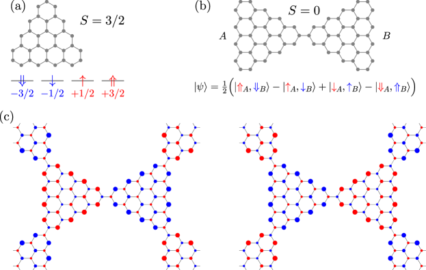
Figure 1: (a) [4]triangulene has a fourfold degenerate ground state with total spin $S=3/2$. (b) [4]triangulene dimer is an open-shell singlet with an entangled wave function as a result of antiferromagnetic intermolecular coupling. (c) Two examples of broken-symmetry Néel states for [4,4]triangulene 2D crystals, obtained with a collinear mean-field Hubbard model. The size of the circles represents the magnitude of the local moments, with red/blue colors denoting spin-$\uparrow$/$\downarrow$. Total spin is no longer a good quantum number.

In this work, we undertake a systematic study of the electronic properties of triangulene 2D crystals, focusing on the magnetic properties of their ground states. To do so, we go beyond the spin-restricted framework in the case of DFT, and beyond non-interacting tight-binding models. For that matter, we take the natural next step, doing spin-unrestricted DFT calculations and adding a Hubbard term to the tight-binding model used in previous work. The Hubbard model is treated at three levels of approximation: collinear mean-field theory, random phase approximation (RPA) and exact diagonalization of small structures in a restricted space of configurations, the so-called complete active space (CAS) method.

Previous spin-unrestricted DFT calculations predict that [2,2]- (ref.Zhou and Liu (2020)) and [3,3]- (ref.Ortiz et al. (2022)) triangulene 2D crystals should display antiferromagnetic order, with the two sublattices being polarized in opposite directions. The [4,4]triangulene crystal is different from [2,2] and [3,3] as it features a small band-gap when calculated both with spin-restricted DFTSethi et al. (2021); Ortiz et al. (2022); Delgado et al. (2023) and with the conventional single-orbital tight-binding model with third-neighbor hoppingOrtiz et al. (2022). On the basis of this narrow gap, an excitonic insulating phase has been proposedSethi et al. (2021), taking as a reference-state the closed-shell non-magnetic ground state. A major goal of this manuscript is to address whether the [4,4]triangulene crystal also features an antiferromagnetic phase (Fig. 1c), and how this affects the size of the gap and the putative excitonic insulator.

The rest of the paper is organized as follows. In section II we review the different theoretical methods used in this work. In section III we present our results for triangulene dimers within the CAS approach for the Hubbard model. These calculations allow us to derive the effective spin interactions, in the form of polynomials of the Heisenberg coupling, and to estimate the magnitude of the intermolecular exchange couplings. In section IV we present the results of collinear mean-field Hubbard and spin-unrestricted DFT calculations. The results are very similar, validating the Hubbard model, and systematically predict broken-symmetry magnetic phases as the ground state of triangulene 2D crystals. In section V we present our Hubbard model RPA calculations of the spin waves for the [2,3], [3,3] and [4,4] crystals, and compare them with those obtained from the spin models derived from the Hubbard model CAS calculations. In section VI we discuss how the lack of contrast in the local density of states (LDOS) of the conduction and valence bands can be used to identify the emergence of broken-symmetry states, providing an explanation to recent experimental scanning tunneling microscope (STM) spectroscopy resultsDelgado et al. (2023). In section VII we present the conclusions.

II Methods

In this section we provide a brief description of the theoretical methods used throughout the paper.

II.1 Hubbard model

Following previous workFujita et al. (1996); Wakabayashi et al. (1998); Peres et al. (2004); Fernández-Rossier and Palacios (2007); Fernández-Rossier (2008), we use a single-orbital Hubbard model to describe $\pi$-magnetism in graphene nanostructures. The Hubbard modelArovas et al. (2022) can be written as

$${\cal H}=\sum_{i,j,\sigma}t_{i,j}c^{\dagger}_{i\sigma}c_{j\sigma}+U\sum_{i}n_{i\uparrow}n_{i\downarrow},$$ (1)

where the indices $i,j$ run over carbon atoms, $t_{i,j}$ stands for the hopping between sites $i$ and $j$, $U$ is the on-site Hubbard repulsion, $c^{\dagger}_{i\sigma}$ ($c_{i\sigma}$) denotes the operator that creates (annihilates) an electron in site $i$ with spin projection along a quantization axis $\sigma=\uparrow,\downarrow$, and $n_{i\sigma}=c^{\dagger}_{i\sigma}c_{i\sigma}$ is the corresponding number operator. While the first term in the Hamiltonian describes hopping between different sites, the second deals with the intra-atomic Coulomb repulsion cost associated to having a given site (or, more formally, the corresponding $p_{z}$-orbital) doubly occupied.

Unless stated otherwise, we consider systems at half-filling and assume that all $t_{i,j}$ are zero except when $i$ and $j$ are first or third neighbors. We denote first and third neighbor hoppings by $t$ and $t_{3}$, respectively. Second-neighbor hopping $t_{2}$ introduces charge inhomogeneities that are penalized by the Hartree interaction, so that best agreement with DFT is obtained by assuming $t_{2}=0$. Throughout this paper we set $t=-2.7$ eV and $t_{3}$ is taken as a free parameter. For triangulene 2D crystals, good agreement with DFT calculations is obtained if we take $t_{3}\simeq 0.1t$ (ref.Ortiz et al. (2022)).

II.2 CAS

Due to the exponential increase in complexity as the size of a quantum system grows, exact diagonalization of many-body problems is only possible for rather small systems. To treat larger systems, approximate solutions have to be introduced, one of them being the configuration interaction method in the CAS approximation. Here, we follow the implementation of the CAS method for the Hubbard model presented in previous works by some of usOrtiz et al. (2019); Mishra et al. (2021b); Jacob et al. (2021); Jacob and Fernández-Rossier (2022). First, the single-particle spectrum of a given triangulene structure is obtained. Then, a subset of $N_{\text{MO}}$ molecular orbitals (MOs)—containing the zero modes and closest states in energy—is selected, and a complete set of multi-electronic configurations with $N_{e}$ electrons occupying these $N_{\text{MO}}$ MOs is considered; the rest of the electrons are assumed to fully occupy the MOs below the active space. The Hubbard Hamiltonian is represented in this restricted basis set and diagonalized numerically. Hereinafter, we shall refer to this procedure as CAS($N_{\text{MO}}$, $N_{e}$). Since there is one electron per $\pi$-orbital for triangulenes at charge neutrality, we always consider $N_{e}=N_{\text{MO}}$.

II.3 Mean-field

In contrast with the CAS method, the mean-field approximation for the Hubbard model makes it possible to include all the single-particle states of molecules and crystals, but interactions are treated approximately. The mean-field theory can be formulated variationally, where the many-body wave function is written in terms of a set of independent electrons that occupy the energy levels of a mean-field Hamiltonian. Here, we impose that the total $S_{z}$ is a good quantum number, thus breaking the spin-rotation invariance present in the original Hubbard model; this is the so-called collinear mean-field approximation, extensively used in the modelling of magnetism in graphene nanostructuresFujita et al. (1996); Wakabayashi et al. (1998); Fernández-Rossier and Palacios (2007); Palacios et al. (2008); Fernández-Rossier (2008); Yazyev (2008); Jung and MacDonald (2009); Feldner et al. (2010); Soriano and Fernández-Rossier (2012); Ijäs et al. (2013); Ortiz et al. (2018); Zheng et al. (2020). In this case, the Hamiltonian takes the form:

$$\begin{split}{\cal H}&=\sum_{i,j,\sigma}t_{i,j}c^{\dagger}_{i\sigma}c_{j\sigma}\\ &\quad+U\sum_{i}\left(\langle n_{i\uparrow}\rangle n_{i\downarrow}+\langle n_{i\downarrow}\rangle n_{i\uparrow}-\langle n_{i\uparrow}\rangle\langle n_{i\downarrow}\rangle\right),\end{split}$$ (2)

where the local densities $\langle n_{i\sigma}\rangle$ are computed with the variational wave function. Therefore, the variational wave function and the mean-field Hamiltonian have to be determined in a self-consistent manner. In practice, this is done by iteration, starting from an initial guess for the local densities. In crystals, the local densities are also periodic so that the eigenvalues and eigenvectors of Eq. (2) satisfy Bloch’s theorem and can be classified in terms of a wave vector $\bm{k}$.

In general, we classify the collinear mean-field solutions in two groups: broken-symmetry solutions for which the expectation values of the local spin operators are finite, and non-magnetic solutions, that are isomorphic to the non-interacting case, except from a trivial rigid shift of the energies. Therefore, the mean-field method provides the value of $S_{z}$ that minimizes the energy, the expectation value of the local moments, and a set of energy levels. These three quantities can be compared with DFT. In the case of graphene nano-islandsFernández-Rossier and Palacios (2007) and ribbonsFujita et al. (1996); Son et al. (2006); Fernández-Rossier (2008), the predictions of mean-field theory were found to be in good agreement with those of DFT for some values of $U$. For triangulene 2D crystals we also find a good agreement. Therefore, comparison of DFT and mean-field Hubbard models allows us to obtain an educated guess for $U$ in these systems.

In our mean-field calculations for 2D triangulene crystals, we have considered a $5\times 5$ Monkhorst–Pack grid for the $\bm{k}$-point sums and a tolerance of $10^{-4}$ for convergence in the local densities. Different initial guesses for the local densities were tested, with the antiferromagnetic guess found to yield the lowest energy solution in all relevant cases.

II.4 RPA

In order to study spin excitations of 2D triangulene crystals, we use the standard RPA to calculate their transverse spin susceptibility matrix for wave vector $\bm{Q}$ and frequency $\Omega$ (refs.Wakabayashi et al. (1998); Barbosa et al. (2001); Peres et al. (2004); Culchac et al. (2011)),

$$\chi_{ii^{\prime}}(\bm{Q},\hbar\Omega)=\frac{1}{N}\sum_{\bm{R}}\mathrm{e}^{\mathrm{i}\bm{Q}\cdot\bm{R}}\int_{-\infty}^{\infty}\mathrm{d}\mathrm{t}\ \mathrm{e}^{-\mathrm{i}\Omega\mathrm{t}}\chi_{ii^{\prime}}(\bm{R},\mathrm{t}),$$ (3)

which is the space and time Fourier transform of the spin-flip Green function,

$$\chi_{ii^{\prime}}(\bm{R}-\bm{R}^{\prime},\mathrm{t})=-\mathrm{i}\theta(\mathrm{t})\left\langle[S^{+}_{\bm{R},i}(\mathrm{t}),S^{-}_{\bm{R}^{\prime},i^{\prime}}(0)]\right\rangle,$$ (4)

where $i,i^{\prime}$ are atomic site indices within a unit cell, $\hbar$ is the reduced Planck constant, $N$ is the number of unit cells, $\bm{R},\bm{R}^{\prime}$ denote unit cell positions, $S^{+}_{\bm{R},i}(\mathrm{t})$ is the time-dependent version (in the Heisenberg picture) of the spin ladder operator $S^{+}_{\bm{R},i}\equiv c^{\dagger}_{\bm{R},i,\uparrow}c_{\bm{R},i,\downarrow}$ at time $\mathrm{t}$, $S^{-}\equiv(S^{+})^{\dagger}$, $\theta(\mathrm{t})$ is the unit step function, and $[\cdot,\cdot]$ denotes the commutator. The spin-flip Green function depends only on the relative position of unit cells $\bm{R}-\bm{R}^{\prime}$ due to the translation symmetry of the crystal.

Within the RPA, we first obtain the mean-field susceptibility $\chi^{0}$, which corresponds to taking the average $\langle\cdot,\cdot\rangle$ over a self-consistent mean-field state associated with the Hamiltonian given in Eq. (2). Then the “interacting” susceptibility can be calculated using the RPA equation,

$$\begin{split}\chi_{ii^{\prime}}(\bm{Q},\hbar\Omega)&=\chi^{0}_{ii^{\prime}}(\bm{Q},\hbar\Omega)\\ &\quad-U\sum_{i^{\prime\prime}}\chi^{0}_{ii^{\prime\prime}}(\bm{Q},\hbar\Omega)\chi_{i^{\prime\prime}i^{\prime}}(\bm{Q},\hbar\Omega),\end{split}$$ (5)

which can be cast in the following matrix form:

$$[\chi]=(\mathds{1}+U[\chi^{0}])^{-1}[\chi^{0}],$$ (6)

where $[\chi]$ contains the matrix elements $\chi_{ii^{\prime}}(\bm{Q},\hbar\Omega)$, and analogously for $[\chi^{0}]$. The specific mean-field susceptibilities that are relevant to us are given by Lindhard-like expressions,

$$\begin{split}\chi^{0}_{ii^{\prime}}(\bm{Q},\hbar\Omega)=\\ \frac{1}{N}\sum_{\bm{k}}\sum_{\lambda,\lambda^{\prime}}\psi_{\bm{k},\lambda,\uparrow}(i^{\prime})\psi^{*}_{\bm{k},\lambda,\uparrow}(i)\psi_{\bm{k}+\bm{Q},\lambda^{\prime},\downarrow}(i)\psi^{*}_{\bm{k}+\bm{Q},\lambda^{\prime},\downarrow}(i^{\prime})\times\\ \times\frac{f(E_{\bm{k},\lambda,\uparrow})-f(E_{\bm{k}+\bm{Q},\lambda^{\prime},\downarrow})}{\hbar\Omega+E_{\bm{k},\lambda,\uparrow}-E_{\bm{k}+\bm{Q},\lambda^{\prime},\downarrow}+\mathrm{i}\eta},\end{split}$$ (7)

where $\psi_{\bm{k},\lambda,\sigma}(i)$ is the wave function coefficient, at site $i$, of a Bloch eigenstate of band $\lambda$ with wave vector $\bm{k}$ and spin $\sigma$ of the mean-field Hamiltonian. The associated eigenvalues are $E_{\bm{k},\lambda,\sigma}$, and $f(E)$ is the Fermi-Dirac distribution function. The sum over $\bm{k}$ spans the Brillouin zone of the crystal. To calculate $\chi^{0}_{ii^{\prime}}(\bm{Q},\hbar\Omega)$, we have used 2500 reciprocal space points within the Brillouin zone of the crystal (equivalent to considering $N=2500$ unit cells), which guarantees convergence of the $\bm{k}$-space sum. All the results are obtained at zero temperature. An empirical broadening of the single-particle states $\eta=5$ meV has been adopted.

The RPA expression for $\chi$ also allows to determine the critical value of $U$, denoted by $U_{c}$, above which the non-magnetic solutions are no longer stable. The magnetic instability is signaled by the condition $\det(\mathds{1}-U_{c}[\chi^{0}])=0$, with $[\chi^{0}]$ calculated at $\Omega=0$ for the Hamiltonian in Eq. (2) with $U=0$. The kind of spin arrangement towards which the true self-consistent mean-field solution tends, either ferromagnetic or antiferromagnetic, is indicated by the wave vector $\bm{Q}$ at which the condition is satisfied for the smallest $U_{c}$, together with the eigenvector of $[\chi^{0}]$ corresponding to its largest eigenvalue Moriya (1985).

II.5 DFT

The DFT calculations have been performed with the local-density approximation, as implemented in Quantum EspressoGiannozzi et al. (2009). We have used norm-conserving pseudopotentials, with a kinetic energy cutoff of 50 Ry and a $\bm{k}$-point sampling of $12\times 12\times 1$ in a Monkhorst-Pack mesh. To avoid spurious interaction between replicas we have set a vacuum distance of 20 $\mathrm{\text{Å}}$. We have set the same experimental lattice parameter and atomic positions for the three cases of magnetic order (non-magnetic, ferromagnetic and antiferromagnetic). The optimized atomic positions have been calculated using the non-magnetic phase and the final structure is planar.

II.6 LDOS

The LDOS at energy $E$ and position $\bm{r}=(x,y,z)$ was calculated using the following equation:

$$\text{LDOS}(E,\bm{r})=\sum_{\bm{k},\lambda,\sigma}|\phi_{\bm{k},\lambda,\sigma}(\bm{r})|^{2}\delta(E-E_{\bm{k},\lambda,\sigma}).$$ (8)

The delta function was approximated by a Lorentzian of the form

$$\delta(E-E_{\bm{k},\lambda,\sigma})\simeq\frac{1}{\pi}\frac{\Gamma}{\Gamma^{2}+(E-E_{\bm{k},\lambda,\sigma})^{2}},$$ (9)

where $\Gamma$ is the half width at half maximum of the Lorentzian function. In our calculations, we took $\Gamma=8$ meV and used a $5\times 5$ Monkhorst–Pack grid for the $\bm{k}$-point sum. Moreover, we considered a carbon Slater distribution for the $2p_{z}$ atomic wave function,

$$\phi_{\bm{k},\lambda,\sigma}(\bm{r})\propto\sum_{\bm{R}}\mathrm{e}^{\mathrm{i}\bm{k}\cdot\bm{R}}\sum_{i}\psi_{\bm{k},\lambda,\sigma}(i)z\mathrm{e}^{-\frac{|\bm{r}-\bm{R}_{i}|}{r_{0}}},$$ (10)

with $r_{0}=0.325~{}$\mathrm{\text{Å}}$$ (refs.Slater (1930); Jacob et al. (2021)). For clarity, $\bm{R}$ denotes a lattice vector and $\bm{R}_{i}$ is the specific position of site $i$ in the corresponding unit cell.

III Hubbard model CAS calculations for centrosymmetric dimers

In this section we present the results of CAS calculations for $[n]$triangulene dimers. The main goal here is to show that, for $U/|t|\gtrsim 1$, the low-energy spectrum can be mapped to a spin model, providing evidence that the dimers remain open-shell and the triangulenes preserve their magnetic moments. We focus on the cases of $n=4$ and $n=3$ dimers, as the $n=2$ case has been already studied in detail in previous workJacob and Fernández-Rossier (2022).

According to the theorem for the number of zero modes in sublattice-imbalanced bipartite lattices, one should find (at least) $n-1$ zero-energy states for an individual $[n]$triangulene moleculeSutherland (1986); Ortiz et al. (2019). In contrast, $[n]$triangulene dimers have a null sublattice imbalance, so they may have no zero modes. However, we findOrtiz et al. (2022) that there are $2(n-1)$ states close to zero energy, on account of the vanishing weight of the zero modes on the intermolecular binding sites. Only third-neighbor hopping leads to a small intermolecular hybridization of the triangulene zero modesOrtiz et al. (2022).

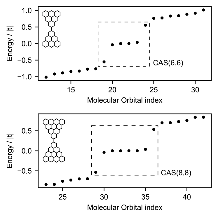
Figure 2: Single-particle energy levels of [3]triangulene (top) and [4]triangulene (bottom) dimers, and the respective active space used in the CAS calculations. Results obtained using $t_{3}=t/10$.

In Fig. 2 we show the single-particle spectra for [3]- and [4]triangulene dimers, obtained by solving the Hamiltonian of Eq. (1) with $U=0$ and $t_{3}=t/10$. As expected, for the [3]triangulene dimer we find four states close to zero energy, originating from the weak intermolecular hybridization of the two zero modes hosted by each monomer individually, promoted by third neighbor hopping. For the [4]triangulene dimer, a similar result is found, only this time the three zero modes of the monomers hybridize to give six states close to zero energy. We also depict the choice of MOs that will enter in the CAS calculation for each of the molecules. These active spaces were chosen to include an additional pair of orbitals besides the zero modes, as this is crucial to account for the Coulomb-driven superexchange mechanismJacob and Fernández-Rossier (2022).

We now discuss our CAS calculations for the [3]- and [4]triangulene dimers. The results for $U=|t|$ and $t_{3}=t/10$ are presented in panels (a) and (c) of Fig. 3. While the [3]- and [4]triangulene monomers are sublattice imbalanced, which according to Lieb’s theorem implies a ground state with finite total spin ($S=1$ and $S=3/2$, respectively), for $[n]$triangulene dimers the sublattice imbalance vanishes and the ground state has $S=0$. For the $n=3$ dimer, this ground state is followed by a triplet ($S=1$) and a quintet ($S=2$). For the $[4]$ triangulene dimer, an additional septet ($S=3$) follows the $S=1$ and $S=2$ manifolds.

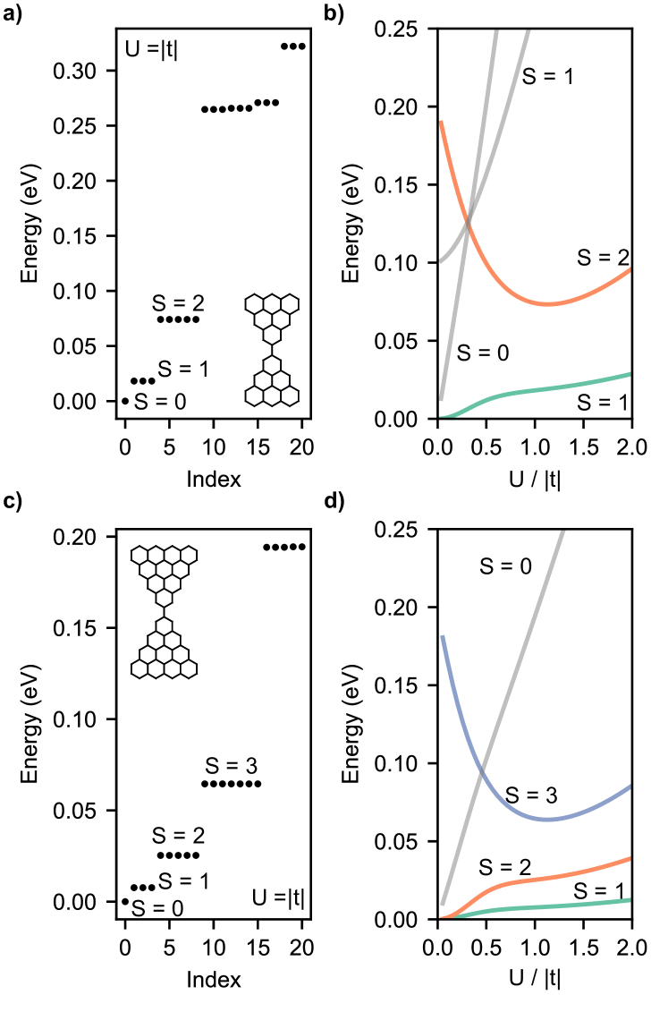
Figure 3: Results obtained with CAS for [3]triangulene (a,b) and [4]triangulene (c,d) dimers. Panels (a) and (c) show the energy of the many-body states, obtained with $U=|t|$ and $t_{3}=t/10$. Panels (b) and (d) show the energy difference between the ground state and the first few excited states, as a function of $U$, for $t_{3}=t/10$.

In panels (b) and (d) of Fig. 3, we show the CAS results for different values of $U$, thus allowing to study how the energies of the many-body states are affected by the strength of the on-site Coulomb repulsion. Inspecting this figure, it becomes clear that, for $U\gtrsim|t|$, the low-energy excitation order $S=1$, $S=2$ (and $S=3$ for the [4]triangulene dimer) is preserved and, crucially, remains well separated from higher-energy excitations. As $U$ is reduced, however, the low-lying excitations become closer to the high-energy ones, and for a critical value of $U$ a crossover is visible.

In the parameter region where the low-energy manifold is well separated from the higher-energy states, the low-energy spectrum of the triangulene dimers can be modeled by a simple spin Hamiltonian where each triangulene is represented by a spin whose value is that of the ground state of the corresponding monomer. To establish a quantitative comparison, we postulate a non-linear Heisenberg dimer Hamiltonian,

$$H=J\left[\vec{S}_{A}\cdot\vec{S}_{B}+\beta_{2}\left(\vec{S}_{A}\cdot\vec{S}_{B}\right)^{2}+\beta_{3}\left(\vec{S}_{A}\cdot\vec{S}_{B}\right)^{3}\right],$$ (11)

where $\vec{S}_{A},\vec{S}_{B}$ are the vectors of the spin operators for the individual $[n]$triangulenes, taken to be $S_{A}=S_{B}\equiv s=1$ and $S_{A}=S_{B}\equiv s=3/2$ for $n=3$ and $n=4$, respectively.

In Appendix A, we derive analytical expressions for the energy levels of this Hamiltonian. By matching these expressions with the results found with CAS for the low-energy manifolds of the $[n]$triangulene dimers, we are able to compute $J,\beta_{2},\beta_{3}$ as a function of $U$ and $t_{3}$. As a reference, in Table 1 we give their values for $U=|t|$ and $t_{3}=0.1t$. We see that, for both molecules, the exchange coupling $J$ is in the order of tens of meV, with the $n=3$ dimer presenting the larger antiferromagnetic exchange. In both cases, it is found that the biquadratic term (given by $\beta_{2}J$) is approximately 10% of the bilinear one ($J$), emphasizing its importance to accurately capture the energy levels with a spin model. As for $\beta_{3}$, which is only included in the model of the $n=4$ dimer (as explained in Appendix A), it is found to be one order of magnitude smaller than $\beta_{2}$. Thus, we see that the bicubic term only introduces minor corrections to the energy spectrum, which further justifies not accounting for it to describe the $n=3$ dimers.

The fact that we can map the low-energy levels of the fermionic CAS calculation to a spin model, together with the fact that, for $U\gtrsim|t|$, these are well separated from higher-energy excitations provides a strong evidence that the dimers are in the open-shell regime, the triangulenes host local moments, and the singlet ground state arises from the intermolecular antiferromagnetic coupling. This shows that, although intermolecular hybridization is present, the magnetic nature of the triangulenes is preserved and the intermolecular interactions are antiferromagnetic. A comparison of the intermolecular hybridization and the Coulomb energies is provided in Appendix B. As we decrease $U$, the low-energy excitations and the high-energy ones become closer, and the validity of the model is no longer warranted. The spin model description certainly fails where the crossover between low- and high-energy excitations occursCatarina and Fernández-Rossier (2022).

$n$	$J$ (meV)	$\beta_{2}$	$\beta_{3}$
3	27.9	0.12	-
4	11.3	0.09	0.007

Table 1: Exchange coupling parameters ($J,\beta_{2},\beta_{3}$) obtained by equating the eigenvalues of the non-linear Heisenberg dimer Hamiltonian of Eq. (11) to the CAS results obtained for $[n]$triangulene dimers with $U=|t|$ and $t_{3}=0.1t$.

IV 2D crystals: DFT and mean-field Hubbard model calculations

In this section we undertake the study of magnetic properties in 2D triangulene crystals. For that matter, we compare DFT-based calculations, both spin-restricted and spin-polarized, with mean-field Hubbard model results. We consider ferromagnetic (FM) and antiferromagnetic (AF) broken-symmetry solutions, as well as non-magnetic (NM) states. In all cases considered, we find that the lowest energy configuration corresponds to the AF solution.

IV.1 DFT for the $[4,4]$triangulene crystal

We now discuss the electronic properties of the [4,4]triangulene crystal, as described with DFT-based calculations. We note that both the spin-restricted and the AF cases of the [2,2]- and [3,3]triangulene crystals were addressed in previous worksZhou and Liu (2020); Ortiz et al. (2022). In both systems, it was found that the NM solution is an excited state and describes a zero-gap semiconductor with two Dirac cones and a narrow bandwidth. The spin-polarized AF solution opens up a large gap and is the ground state.

Previous workSethi et al. (2021); Ortiz et al. (2022); Delgado et al. (2023) has shown that the spin-unpolarized [4,4]triangulene crystal is a narrow-gap semiconductor with flat valence and conduction bands. Here, we go beyond the NM framework and study two magnetic phases, AF and FM. We find that the AF phase has smaller energy than both the FM ($E_{FM}-E_{AF}=0.171$ eV) and the NM ($E_{NM}-E_{AF}=0.457$ eV). It is thus apparent that DFT calculations confirm the open-shell nature of the [4]triangulenes when covalently bonded to form a 2D honeycomb crystal. If we model the energy difference between the AF and FM phases with a classical Heisenberg model on a honeycomb lattice, we get $6JS^{2}=0.171$ eV. Using $S=3/2$, we pull out $J=12.7$ meV. For the [3,3]triangulene crystal, a similar analysisOrtiz et al. (2022) found $E^{[3,3]}_{FM}-E^{[3,3]}_{AF}=0.159$ eV and $J^{[3,3]}=26.5$ meV.

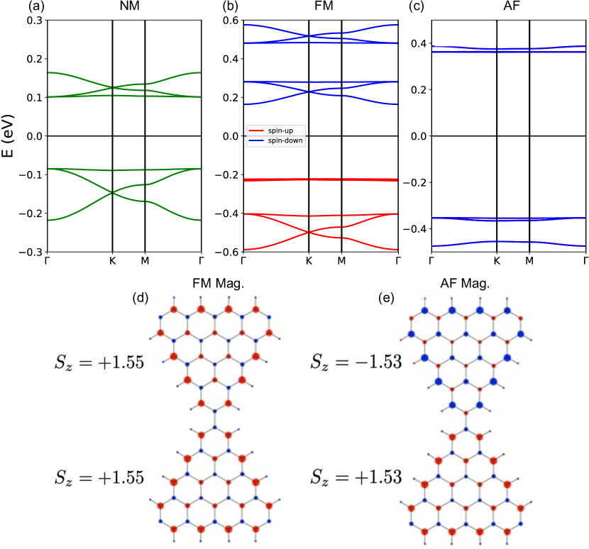
Figure 4: Electronic structure, obtained with DFT, of [4,4]triangulene 2D crystals for the following cases: (a) non-magnetic, (b) ferromagnetic and (c) antiferromagnetic. The corresponding magnetizations of the FM and AF cases are shown in panels (d) and (e), respectively; the value of $S_{z}$ per triangulene is also indicated. Red/blue colors correspond to spin-up/down. In (c), spin-up and spin-down bands are degenerate.

In Fig. 4, we show the energy bands for the three configurations (NM, FM, AF) of the [4,4]triangulene crystal, together with the distribution of the magnetic moments in the FM and AF solutions. The three solutions are gapped, but the size of the gap increases in the magnetic phases, specially in the AF case. The FM bands have a similar line shape than the NM bands, except for the top of the conduction band. The AF bands are much narrower than the NM bands. This relates to the quenching of intermolecular hybridization due to the opposite-sign spin splitting of the zero modes of adjacent molecules.

We note that, whereas the magnetic moments lie predominantly in the majority sublattice of each triangulene, there is a smaller magnetization with opposite sign in the minority sublattice, coming presumably from electrons in non-zero modes. Moreover, we find that the magnetization per triangulene shares a similar pattern for both FM and AF solutions, and the values obtained are compatible with the predictions for individual triangulenes.

IV.2 Mean-field Hubbard model results

We now present our results for the [2,2]-, [2,3]-, [3,3]-, and [4,4]triangulene 2D crystals, obtained using the collinear mean-field approximation to the Hubbard model at half-filling. For the centrosymmetric $[n,n]$trianguelene crystals, we find that, for $U$ above an $n$-dependent critical value $U_{c}(n)$ below which the ground state solutions are NM (see Subsection IV.4), the lowest energy solutions are AF, in agreement with DFT calculations. As for the non-centrosymmetric [2,3] case, the ground state obtained is always ferrimagnetic.

In Fig. 5, we show the energy bands for both NM and ground state (magnetic) configurations, obtained with $U=0$ and $U=|t|$, respectively. Two features are immediately apparent. First, the dispersion of the AF bands is narrower compared to the NM case. This is a consequence of suppressed intermolecular hybridization, on account of the opposite-sign spin splitting in the two triangulenes of the unit cell. Second, the separation between conduction and valence bands increases in the magnetic phases. Thus, the [2,2]-, [2,3]-, and [3,3]triangulene crystals, gapless for $U=0$, become gapped when magnetic order appears. In the case of the [4,4]triangulene crystal, gapped for $U=0$, the interactions increase the gap by more than a factor of 3. The gap of the magnetically ordered phases reflects the fact that every triangulene is full-shell in a spin-channel, so that the addition of a new electron is only possible in the minority spin channel, that became spin-split.

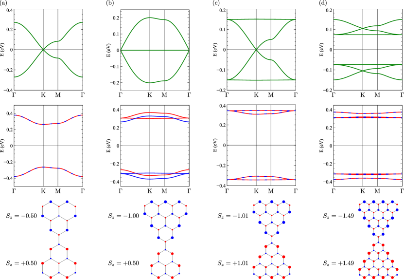
Figure 5: Electronic properties of (a) [2,2]-, (b) [2,3]-, (c) [3,3]- and (d) [4,4]triangulene 2D crystals. Top panels show the NM energy bands, obtained using a tight-binding model with $t_{3}=0.1t$; horizontal black lines denote the Fermi energy. Middle panels show the energy bands of the ground state solution of a collinear mean-field Hubbard model with $U=|t|$; red/blue colors denote spin-up/down. The corresponding magnetizations are shown in the bottom panels, where the size of the circles represents the magnitude of the local moments. The value of $S_{z}$ per triangulene is also indicated.

In Fig. 5, we also show the local magnetic moments corresponding to the ground state mean-field solutions. The magnetization pattern is such that carbon sites in different sublattices are magnetized with opposite sign. For $U\simeq|t|$, the magnetic moments per triangulene are close to the values expected from Lieb’s theorem for individual triangulenes, and in qualitative agreement with those of DFT. We note that mean-field theory is not constrained by Lieb’s theorem, that applies to exact solutions.

For the non-centrosymmetric [2,3]triangulene crystal, the magnetic order appears for arbitrarily small values of $U$. This is expected on account of the flat band at the Fermi energy. For small values of $U$, magnetic moments are only present in the larger unit, that hosts the flat-band states. As $U$ is ramped up, the magnitude of the magnetic moments in both units increases towards values close to those of the isolated triangulenes, and a ferrimagnetic ground state is obtained.

IV.3 Comparison between mean-field and DFT

In this section, we briefly compare the results of the mean-field Hubbard models with those of DFT, for the $[2,2]$, $[3,3]$ and $[4,4]$ crystals. The DFT results for the $[2,2]$ crystals are taken from ref.Zhou and Liu (2020). As for the [3,3] crystals, DFT calculations were reported in ref.Ortiz et al. (2022) by two of us. Since the comparison of the NM phases was already established in previous workOrtiz et al. (2022), we focus on the magnetic phases.

Qualitatively, both levels of theory are in agreement. They both predict AF solutions as the ground state, with magnetic moments close to those predicted for isolated triangulenes. Moreover, both in mean-field and DFT the band-gap of the magnetic solutions is much larger than the NM cases, and the band dispersion is narrower.

Given the uncertainty over the best value of $U$, we make no attempt to find the value of $U$ for which this agreement is better, and we take $U=|t|$ as a reasonable guess. It is apparent that the mean-field bands obtained with $U=|t|$ are in good agreement with the DFT calculations. The same is also verified for the magnetization patterns (see figures (4)d,e and lower panels (5). A quantitative comparison between the mean-field theory for $U=|t|$ and DFT is provided in Table 2. We find a fairly good agreement that justifies the use of Hubbard models for this type of system. Specifically, for the $[4,4]$ case, we obtain a good agreement in: (i) the energy difference between the different magnetic phases (with the NM configuration featuring the highest energy of the three); (ii) the band gaps of the NM and AF solutions, with both levels of theory predicting an increase of the band gap by a similar factor in the AF phase; (iii) the $S_{z}$ per triangulene (discussed above); (iv) the absolute value of the magnetization, defined by $|M_{\text{tot}}|=g\mu_{\text{B}}\sum_{i}|S_{z}(i)|$, where $g=2$ is the electron $g$-factor and $\mu_{\text{B}}$ stands for the Bohr magneton.

System	Quantity	DFT	Mean-field
$[2,2]$	$E_{FM}-E_{AF}$ (eV)	0.11a	0.109
$[2,2]$	$E_{NM}-E_{AF}$ (eV)	0.12a	0.097
$[3,3]$	$E_{FM}-E_{AF}$ (eV)	0.159b	0.137
$[4,4]$	$E_{FM}-E_{AF}$ (eV)	0.171	0.133
$[4,4]$	$E_{NM}-E_{AF}$ (eV)	0.457	0.508
NM $[4,4]$	Gap (eV)	0.185	0.148
AF $[4,4]$	Gap (eV)	0.716	0.625
AF $[4,4]$	$|M_{\rm tot}|$ ($\mu_{\text{B}}$)	8.89	9.01
AF $[4,4]$	$S_{z}$ per triangulene	1.53	1.49

Table 2: Agreement between DFT and mean-field Hubbard model calculations for different magnetic phases of $[n,n]$triangulene 2D crystals. Mean-field results were obtained with $t_{3}=0.1t$ and $U=|t|$. ^a: Ref.Zhou and Liu (2020); ^b: Ref.Ortiz et al. (2022).

IV.4 Critical value of $U$

We now discuss the minimal value of $U$ that makes the NM solution unstable within the mean-field Hubbard approximation. This can be obtained in two ways. First, by comparing the NM and the magnetic solutions of a mean-field calculation as a function of $U$ and finding the critical value $U_{c}$ above which the disordered phase becomes an excited state. Second, a faster approach, discussed in Section II.4 and adopted here, where we look for the value $U=U_{c}$ for which the non-interacting RPA susceptibility diverges. The results are shown in Fig. 6 for the $[n,n]$ crystals with $n=2,3,4$. We note that, for a honeycomb Hubbard model at half-filling, the mean-field critical value for the NM to AF transition is $U_{c}=2.2|\tau|$ (ref. Sorella and Tosatti (1992)), where $\tau$ is the first neighbor hopping of the honeycomb lattice.

For the $[2,2]$triangulene crystal, whose low-energy single-particle Hamiltonian maps exactly to that of a honeycomb modelOrtiz et al. (2022), the effective first neighbor hopping is given by $\tilde{t}=|t_{3}|/3$ and the effective Hubbard interaction is $\tilde{U}=U/6$ (ref.Ortiz et al. (2022)). Therefore, by renormalizing the $U_{c}=2.2|\tau|$ equation, we can estimate a critical value $U_{c}=4.4|t_{3}|$ for the [2,2] crystal, in good agreement with the $U_{c}$ numerically obtained (see Fig. 6).

Given that the low-energy spectrum of the $[3,3]$triangulene crystal also features graphene-like bands in the neighborhood of the Fermi energy, we can also compare the numerically obtained $U_{c}$ with that of the honeycomb crystal. For the $[3,3]$ crystal, the effective first neighbor hopping is given by $\tilde{t}=2|t_{3}|/11$ and the effective Hubbard is $\tilde{U}\simeq U/11$ (ref.Ortiz et al. (2022)). Therefore, we also estimate a critical value $U_{c}\simeq 4.4|t_{3}|$. The fact that our numerical estimates for $U_{c}(t_{3})$ are slightly different (see Fig. 6) reflects the fact that $U_{c}$ is also influenced by the flat bands away from the Fermi energy.

The critical values of $U$ for $t_{3}=0.1t$ are in the range of $U_{c}\lesssim 0.45|t|<1.2$ eV. Estimates of atomic $U$ for carbon are higher than this, in the range of 3.5 eV (ref.Yazyev (2010)). Mean-field theories are known to underestimate $U_{c}$. For instance, Quantum Monte Carlo methodsSorella and Tosatti (1992) predict $U_{c}=4.5|\tau|$ for the Hubbard model on the honeycomb lattice. Even if $U_{c}$ is twice as large as the values predicted by mean-field, magnetic order should appear in the triangulene crystals.

Interestingly, the value of $U_{c}$ is very similar for the $[3,3]$ and $[4,4]$ crystals. This result further supports the picture that, once moderately large interactions are included, the fact that the NM bands of the $[4,4]$ crystal have a band-gap does not seem to have a dramatic effect on its electronic properties, and the $[4,4]$triangulene crystal is (antiferro) magnetic.

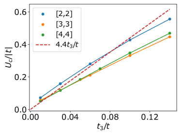
Figure 6: Critical values $U_{c}$ of the Hubbard parameter for the onset of the magnetic instability, as predicted by the RPA, as a function of the third neighbor hopping $t_{3}$, for the [2,2]-, [3,3]- and [4,4]triangulene crystals.

V Collective spin excitations in 2D triangulene crystals

V.1 RPA for the Hubbard model

The choice of a “ground state” with broken spin rotation symmetry implies the existence of gapless Goldstone modes, the spin waves. Here we obtain the spin wave spectra of 2D triangulene lattices by computing the transverse spin susceptibility $\chi(\boldsymbol{Q},\hbar\Omega)$ of the Hubbard Hamiltonian (Eq. (1)) in the RPA, as discussed in Section II.4. The spin wave frequencies are associated with the poles of $\chi(\boldsymbol{Q},\hbar\Omega)$. For a given wave vector, two poles occur at energies $\pm\hbar\Omega(\boldsymbol{Q})$, due to the opposite directions of the spins in the two magnetic sublattices.Fisher (1971) From those we can build a spin wave dispersion relation, shown in Figs. 7a,b for the $[3,3]$ and $[4,4]$ crystals, and in Fig. 7c for the $[2,3]$ crystal. We note that, for the centrosymmetric cases ($[3,3],[4,4]$), the two modes are degenerate, in contrast with the $[2,3]$ for which we find an acoustic and an optical branch of spin waves. In these figures, the symbols represent the locations of the poles of $\chi(\boldsymbol{Q},\hbar\Omega)$ for a few wave vectors along two high-symmetry directions in the honeycomb Brillouin zone. It is apparent that the bandwidth of the magnon spectrum is larger for the $[3,3]$ crystal, in agreement with the larger values of intermolecular exchange obtained with the CAS calculations for the dimers.

V.2 Comparison with spin models

We now compare the RPA results with those of a Heisenberg spin model with first-neighbor exchange $J$, calculated in the linear spin-wave approximationHolstein and Primakoff (1940); Auerbach (1998). The calculation (not shown) is standardAuerbach (1998). The spin operators are expressed in terms of Holstein-Primakoff (HP) bosonsHolstein and Primakoff (1940), taking the quantization axis parallel to the classical ground state (AF for the $[3,3],[4,4]$, ferrimagnet for the $[2,3]$), where the classical magnetization of each $[n]$triangulene is $2S=n-1$. The resulting bosonic Hamiltonian is truncated so that only terms bilinear in the HP bosons are kept. This bilinear Hamiltonian can be solved exactly, by means of a paraunitary canonical transformation. For a lattice with two spins per unit cell, such as the honeycomb, two spin-wave branches are obtained, given by:

$$\frac{\epsilon_{\pm}(\boldsymbol{k})}{3J}=\frac{S_{A}+S_{B}}{2}\sqrt{1-\xi_{\boldsymbol{k}}}\pm\frac{S_{B}-S_{A}}{2},$$ (12)

where $\xi_{\boldsymbol{k}}=4S_{A}S_{B}|\phi_{\boldsymbol{k}}|^{2}/(S_{A}+S_{B})^{2}$, $S_{A}$ and $S_{B}$ denote the spin of the triangulenes in sublattice $A$ and $B$, $3\phi_{\boldsymbol{k}}=1+\mathrm{e}^{\mathrm{i}\boldsymbol{a}_{1}\cdot\boldsymbol{k}}+\mathrm{e}^{\mathrm{i}\boldsymbol{a}_{2}\cdot\boldsymbol{k}}$, $\boldsymbol{a}_{1,2}$ are the lattice vectors of the honeycomb lattice and $J$ is the intermolecular exchange. It is apparent that in the AF case we have $S_{A}=S_{B}$ and the two branches become degenerate. It is also apparent that, for $\boldsymbol{k}=(0,0)$, the lower energy branch vanishes, complying with the Goldstone theorem.

In Figs. 7a–c, we compare the magnon dispersion calculated from the fermionic RPA theory with the spin wave dispersion of Eq. (12) . Taking $S$ from the mean-field calculation, we determine the value of intermolecular exchange $J$ that provides the best fitting to the RPA calculation within the fermionic model. We find that the RPA curves lies exactly on top of the spin-wave curves, providing additional support to the notion that the low-energy exciations of 2D triangulene crystals can be described with spin model Hamiltonians, very much like the one-dimensional triangulene spin chain.

We can determine the dependence of $J$ on $U$ and $t_{3}$ by repeating this procedure for different values of those parameters. In Fig. 8 we plot $J$, so obtained, as a function of $U/|t|$ with $t_{3}=t/10$ for the $[3,3]$ and $[4,4]$ cases. The general behavior is qualitatively very similar to the results from CAS calculations for dimers, as seen in Figs. 10a,c. In fact, even the actual values of $J$ given by RPA and CAS are reasonably similar for $0.5\lesssim U/|t|\lesssim 1.5$. This qualitative good agreement backs-up the robustness of the main underlying picture of this work: despite the intermolecular hybridization between triangulenes in the 2D crystals considered here, they retain their magnetic moment.

	DFT	Mean-field	CAS	RPA
$J^{[3,3]}$ (meV)	26.5 a	22.8	27.9	20.8
$J^{[4,4]}$ (meV)	12.7	9.9	11.3	8.8

Table 3: Estimates for intermolecular exchange from DFT and from Hubbard model, in three different approximations, taking $U=|t|$, and $t_{3}=0.1t$, for the [3,3] and [4,4] triangulenes. ^a: Ref.Ortiz et al. (2022).

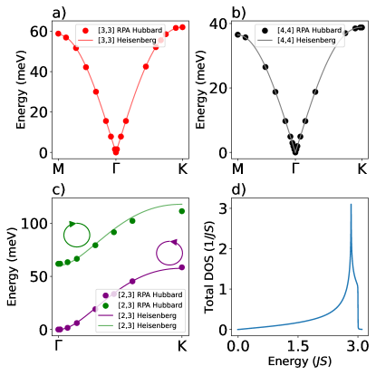
Figure 7: Spin wave dispersion relations within the RPA for $[n,m]$triangulene crystals. a) [3,3] crystal, b) [4,4] crystal, c) [2,3] crystal, for which the two spin wave branches (corresponding to different polarities) are non-degenerate due to the ferrimagnetic nature of the ground state. In contrast, for the $[3,3]$ and $[4,4]$ (antiferromagnetic) crystals, the two polarities are degenerate, thus a single dispersion is shown for each. In a), b) and c) panels, the dots have been extracted from magnon spectral densities (the imaginary part of the transverse spin susceptibility) and the solid curves are fits to nearest-neighbor Heisenberg models. d) Integrated magnon density of states for the nearest-neighbor antiferromagnetic Heisenberg model on the honeycomb lattice, obtained from Eq. (12) with $S_{A}=S_{B}=S$.

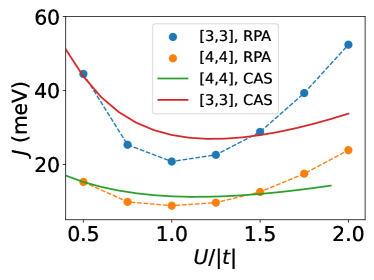
Figure 8: Effective exchange as a function of $U$, obtained by fitting the spin wave dispersion relation to a nearest-neighbor Heisenberg model in the linear spin wave approximation (dots), and from CAS calculations on single dimers (solid curves).

VI Predictions for STM spectroscopy

We now discuss experimental consequences of the magnetic order discussed in the previous sections. Given that, so far, triangulenes structures are studied with STMMishra et al. (2021a); Hieulle et al. (2021); Delgado et al. (2023), we focus properties that can be probed with this technique. STM $dI/dV$ can reveal two different properties of the surfaceOrtiz and Fernández-Rossier (2020): LDOS and inelastic excitations. In the case of nanographenes, LDOS features are revealed as prominent peaks at large voltages, in the range of hundreds of meV, corresponding to resonant tunneling accross specific energy levels of the molecules.

VI.1 Probing LDOS

Here we discuss the LDOS at the energy of the valence and conduction bands, that can be measured by means of STM spectroscopy. The LDOS is sensitive to the interatomic coherence: by virtue of Eq. (8), the LDOS is proportional to the square of the MO wave function, that in turn is a linear combination of atomic orbitals. Therefore, LDOS is sensitive to the relative phases of the weights of the MO at different atoms. Specifically, for the non-interacting bands of a bipartite lattice, electron-hole symmetric states, such as valence and conduction bands have opposite relative phases between adjacent atoms. More formally, let us denote the wave function of a conduction band MO as

$$\psi_{\bm{k},\lambda}(i)=\left(\psi_{\bm{k},\lambda}(A),\psi_{\bm{k},\lambda,\sigma}(B)\right),$$ (13)

where $\psi_{\bm{k},\lambda,\sigma}(A/B)$ encodes the MO weight on all the atoms in the unit cell that belong to the $A$ and $B$ sublattices. Then, for a bipartite lattice, the wave function of the electron-hole conjugate state $\overline{\lambda}$ in the valence band is given bySoriano and Fernández-Rossier (2012)

$$\psi_{\bm{k},\overline{\lambda}}(i)=\left(\psi_{\bm{k},\lambda}(A),-\psi_{\bm{k},\lambda,\sigma}(B)\right)$$ (14)

Thus, electron-hole conjugate MO wave functions have the same probability amplitudes but opposite phases at one sublattice. As a result, LDOS will have a enhancement/depletion at the regions connecting atoms with different sublattices. Specifically, at the bonding region between any pair of atoms, we can truncate Eq. (10) keeping only contribution of the two closest atoms, $a$ and $b$, that, by definition, belong to different sublattices. This leads to

$$\phi_{\bm{k},\lambda}(\bm{r})\simeq\left[\psi_{\bm{k},\lambda}(a)g(\bm{r}-\bm{R}_{a})+\psi_{\bm{k},\lambda}(b)g(\bm{r}-\bm{R}_{b})\right]$$ (15)

where $g(\bm{r}-\bm{R}_{A/B})\equiv z\mathrm{e}^{-\frac{|\bm{r}-\bm{R}_{A/B}|}{r_{0}}}$.

We can now compute the difference of the LDOS computed in the bonding region between two atoms, for which eq. (15) holds, evaluated at energies $+E_{\lambda}$ and $-E_{\lambda}$. The contributions to the difference of LDOS at these two energies from states with the same wave vector $\boldsymbol{k}$ in a pair of electron-hole conjugate bands $\lambda,\overline{\lambda}$ will be given by

$$\delta\rho_{\boldsymbol{k},\lambda}(\bm{r})=4\text{Re}\left[\psi_{\bm{k},\lambda}^{*}(a)\psi_{\bm{k},\lambda}(b)\right]g(\bm{r}-\bm{R}_{a})g(\bm{r}-\bm{R}_{b})$$ (16)

From Eq. (16) it is apparent that the LDOS contrast between electron-hole bands is controlled by the weights (and crucially the respective phases) of the wave functions of the MOs of adjacent atoms (which belong to different sublattices).

In the case of conduction and valence bands of triangulenes, the weight of the wave functions inside each triangulene is all on a single sublattice. Therefore, the LDOS contrast is only seen at the inter-triangulene binding sites. These are shown for the $[4,4]$ triangulene crystal in Fig. 9. For the non-interacting case we find a depletion of the LDOS at the intermolecular binding sites at the conduction band energy and a corresponding enhancement of the valence band (see Fig. 9a,b).

We now discuss how interactions, described at the mean-field level, change this picture. The broken-symmetry Néel states result in the presence of a staggered exchange potential. As a result, for a given spin direction, the on-site energy of two adjacent triangulenes is no longer the same. Consequently, the wave functions of valence and conduction bands no longer have the same weight on both sublattices Soriano and Fernández-Rossier (2012), i.e. Eqs. (13) and (14) relating the wave functions of valence and conduction bands no longer hold. In the interacting cases the MOs become sublattice biased, and in the very strong coupling limit, completely sublattice polarized. This ultimately reduces the amplitude of the bonding-anti-bonding interference effect, as shown in Fig. 9c,d . This is in agreement with the experimental observations of Delgado et al.Delgado et al. (2023).

We note here that the reduction of the LDOS contrast between valence and conduction bands in the interacting cases relates to the reduced bandwidth of the interacting bands. The spin-dependent staggered potential creates an energy barrier for intermolecular hybridization.

In the work of Delgado et al., Delgado et al. (2023), the observed reduced contrast of LDOS at the binding site is attributed to an excitonic insulator state that arises on account of the small gap obtained from the spin-unpolarized DFT calculations. As both our DFT and mean-field results show, the spin polarized solution has lower energy, a larger gap (that makes the excitonic insulator state less likely) and, more important, already accounts for the reduced LDOS contrast in terms of the sublattice symmetry breaking of the AF solution.

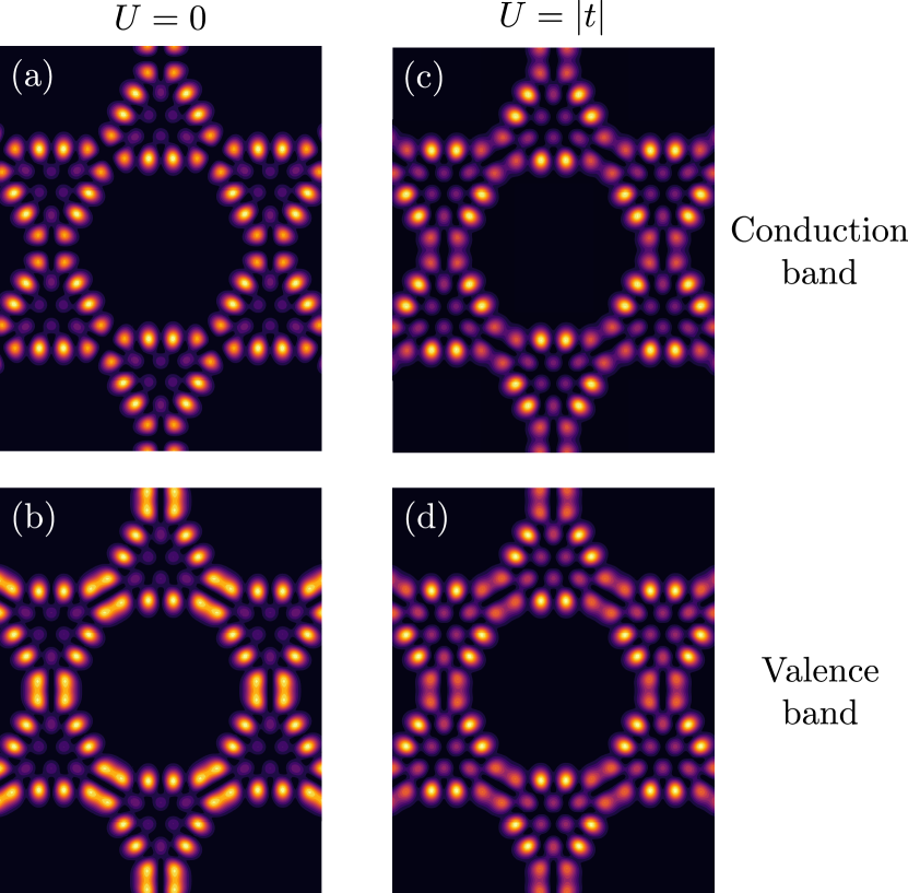
Figure 9: LDOS for [4,4]triangulene 2D crystals. All calculations were performed at height $z=2.8$ $\mathrm{\text{Å}}$. Panels (a,b) show the results obtained with the non-interacting tight-binding model, with $t_{3}=0.1t$, for energies in (a) conduction band ($E=0.1$ eV) and (b) valence band ($E=-0.1$ eV). Panels (c,d) show the results obtained with the collinear mean-field Hubbard model, taking $U=|t|$, for energies in (c) conduction band ($E=0.315$ eV) and (d) valence band ($E=-0.315$ eV).

VI.2 Probing magnons

In contrast to the large-bias LDOS measurements discussed above, STM spectroscopy can reveal inelastic excitations as bias-symmetric steps, at bias voltages below 100 meV, whose height is dramatically smaller than the resonant peaks. The underlying mechanism for these inelastic steps is inelastic cotunneling of electronsDelgado and Fernández-Rossier (2011); Ortiz and Fernández-Rossier (2020). In spin systems, inelastic electron tunneling spectroscopy (IETS) can probe spin transitions between the ground state and excited states that satisfy the rule for the change of total spin $\Delta S=0,\pm 1$. Therefore, IETS is optimal to probe magnonsSpinelli et al. (2014); Klein et al. (2018). We expect that $\frac{d^{2}I}{dV^{2}}$ will have a line shape that reflects the density of states of magnon excitations. In Fig. 7d, we show the magnon LDOS associated to the dispersion energy from Eq. (12) for $S_{A}=S_{B}=S$, relevant for $[n,n]$triangulene crystals. It is apparent that the magnon LDOS features an outstanding Van Hove singularity, at the energy $\sqrt{8}JS$, corresponding to the $M$ points in the Brillouin zone. Therefore, we anticipate the presence of a prominent feature at $eV=\pm\sqrt{8}JS$ energy in the $\frac{d^{2}I}{dV^{2}}$ spectra. For the $[4,4]$triangulene crystal, taking $J\simeq 9$ meV (see Table 3), and $S=3/2$, the steps are expected at $\pm 38$ meV.

VII Summary and conclusions

The main goal of this paper is to describe the consequences of electron-electron interactions in triangulene 2D crystals. Specifically, we address the question of whether triangulenes retain their magnetic moments when forming 2D crystals that entail intermolecular hybridization. This is particularly relevant in the case of $[4,4]$ triangulene crystals, for which the single-particle modelOrtiz et al. (2022) predicts an insulating state that, naively, may quench the emergence of magnetism.

We employ both spin-unrestricted DFT calculations and Hubbard model with three different approximations:

1. Multiconfigurational calculations of triangulene dimers.

2. Mean-field approximation of the 2D crystals, whose results are in qualitative agreement with DFT calculations.

3. RPA calculations of the spin excitations.

Importantly, these different methods permit us to perform cross-validations. For instance, both the spin-polarized DFT and mean-field Hubbard model yield very similar results for all the key quantities (see table 2). The Hubbard-model RPA calculations, building on top of mean-field solutions, predict an excitation spectra that can be fitted very well to a Heisenberg model, with just a single fitting parameter, the effective exchange (see figure (7)a,b,c). In turn, this exchange is in qualitative agreement with the one obtained from CAS calculations, for a range of values of $U$ (see figure (8)).

Our main conclusions are:

1. Triangulenes retain their magnetic moment when forming in two-dimensional crystals, according to both DFT and Hubbard model calculations.

2. Triangulene crystals are insulating, on account of the electron-electron interactions. This is supported both by our mean-field Hubbard model and our spin-polarized DFT calculations. In the case of the $[4,4]$ crystal, the size of the gap, calculated with DFT, comes out 3.9 times larger than the spin-unpolarized gap, which calls for a revision of the predictionsSethi et al. (2021); Delgado et al. (2023) of an excitonic insulator state based on the smaller gap of the non-magnetic ground state.

3. Two-dimensional triangulene crystals are magnetically ordered, either antiferrromagnetically, in the centrosymmetric case, or ferrimagnetically, for non-centrosymmetric crystals. This statement is based on both DFT and mean-field Hubbard calculations.

4. The value $U=|t|$ gives a very good agreement between mean-field Hubbard model and DFT for several quantities, such as the intermolecular exchange, the magnetic moment and the band-gap. We have not tried to fine-tune $U/|t|$ to improve that agreement, but we can be sure that $U\simeq|t|$ is a good ball-park reference for this important ratio, in agreement with previous workMishra et al. (2021a).

5. The low energy spin excitations obtained from the RPA fermionic calculations are very well described with Heisenberg Hamiltonians (see Fig. 7). The exchange interactions so obtained are in qualitative agreement with those obtained from CAS, mean-field and DFT (see table 3).

6. Intermolecular exchange features non-linear interactions, beyond Heisenberg. This is found by comparing CAS calculations for the Hubbard model with spin models. For $U\simeq|t|$, the values of the non-linear terms are in qualitative agreement with previous work for $S=1$Mishra et al. (2021a). For $S=3/2$ triangulenes, the value of the non-linear interactions are very small, so that it is very unlikely that the system realizes the AKLT model for the honeycomb lattice Affleck et al. (1987), that would be for relevant measurement-based quantum computing Wei et al. (2011).

7. Magnetically ordered states reduce the intermolecular hybridization in triangulene 2D crystals. This has two consequences:

   • First, the bandwith of magnetically ordered triangulene crystals are narrower than those of the non-interacting case.

   • Second, a reduction in the difference of the LDOS measured at the valence and conduction band energies at the intermolecular binding sites. This reduction has been observed experimentally in recent work Delgado et al. (2023) in $[4,4]$ triangulene crystals.

We now briefly discuss the robustness of the predicted antiferromagnetic states. By construction, both the mean-field and DFT calculations predict broken-symmetry solutions or non-magnetic solutions. Both quantum and thermal fluctuations can destroy long range order in two dimensions.

At $T=0$, broken symmetry states are robust in this class of system. Using Quantum Monte Carlo, it was shown that the Hubbard model in the honeycomb lattice, at half-filling, features antiferromagnetic long-range orderSorella and Tosatti (1992). Since the effective model for the $[2,2]$ crystal is a Hubbard Hamiltonian that maps into a $S=1/2$ Heisenberg model, given that quantum fluctuations scale with $1/S$, and given that larger triangulenes have larger $S$, we expect that at $T=0$ the ground state of the centrosymmetric triangulene crystals also feature Néel long-range order.

In contrast, thermal fluctuations are expected to destroy long-range order, on account of Mermin-Wagner theoremMermin and Wagner (1966). However, the spin correlation length may be larger than system size for small crystals reported experimentallyDelgado et al. (2023). Therefore, the broken-symmetry solutions remain a good approximation for these systems, as in the case of one-dimensional edge magnetism in graphene ribbonsYazyev and Katsnelson (2008).

Our results, together with previous experimental workMishra et al. (2021b); Delgado et al. (2023), should pave the way for the design of other nanographene molecular crystalsOrtiz et al. (2022, 2023); Ortiz (2023), both 1D and 2D that realize interesting spin Hamiltonians with non-trivial electronic properties.

Appendix A Derivation of spin Hamiltonian parameters

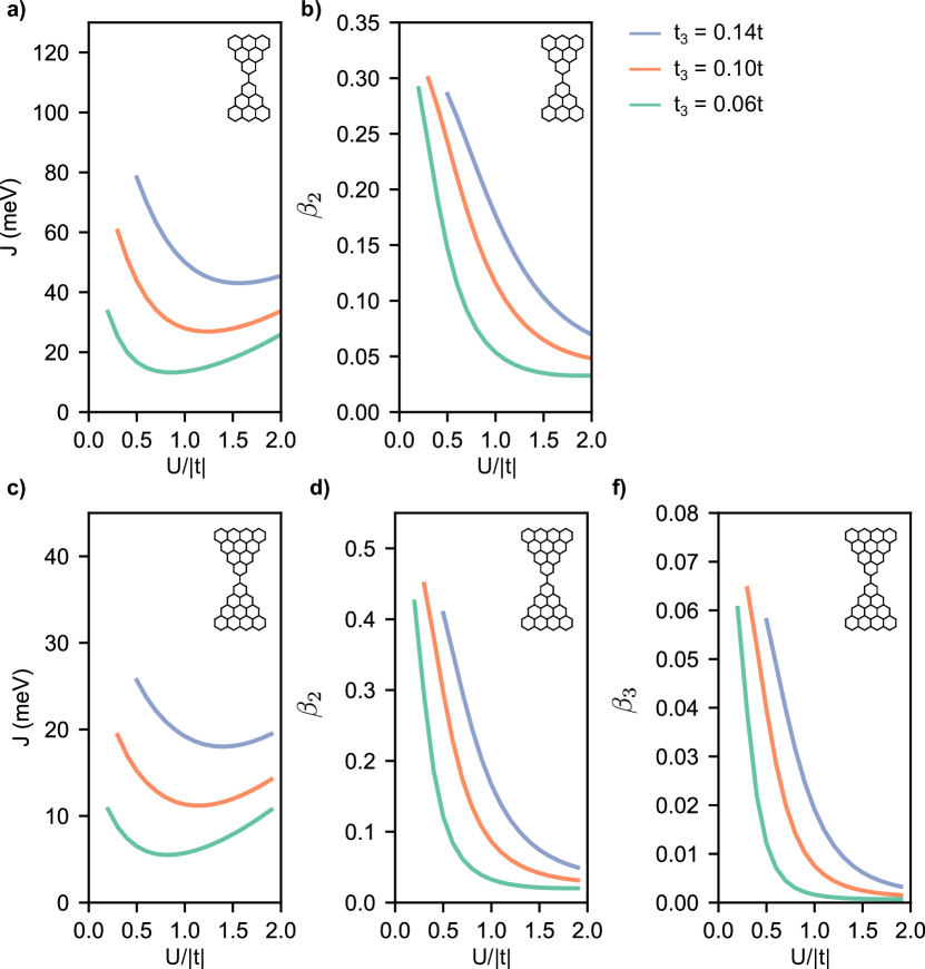
Figure 10: Parameters of the spin model, obtained by matching the spin dimer energy levels to the CAS calculations for triangulene dimers, as a function of $U$, for $t_{3}=0.06t$, $t_{3}=0.1t$ and $t_{3}=0.14t$. Panels (a) and (b) show the results for the [3]triangulene dimer, and panels (c)-(e) show the results for the [4]triangulene dimer.

In this Appendix, we derive the analytical expressions for the energy levels of the spin model dimer Hamiltonian of Eq. (11). Then, by matching these expressions with the numerical results obtained with CAS for $[n]$triangulene dimers, we study how the parameters of the spin model, i.e. $J$, $\beta_{2}$ and $\beta_{3}$, depend on $U$ and $t_{3}$.

In terms of the total spin $S$ and the spin of the triangulenes $s$, the eigenvalues of the spin model of Eq. (11) are given by

$$E_{s}(S)=J\left[f(S,s)+\beta_{2}f(S,s)^{2}+\beta_{3}f(S,s)^{3}\right],$$ (17)

with

$$f(S,s)=\frac{1}{2}\left[S(S+1)-2s(s+1)\right],$$ (18)

where $S$ can take the values $S=0,1,...,2s$. Thus, for the $n=3$ ($n=4$) case, $S$ can take values up to $S=2$ ($S=3$). For the [4]triangulene dimer, the spectrum of the spin model has four multiplets, with $S=0,1,2,3$. For the [3]triangulene dimer, we assume $\beta_{3}=0$ since the $S=1$ dimer model can take the values $S=0,1,2$, and we can only fit two energy parameters out of three multiplets. As we found in previous workMishra et al. (2021b), the model with $\beta_{3}=0$ can account for experimental observations of a large number of structures.

The excitation energies for the $n=3$ case are related to $J$ and $\beta_{2}$ as follows:

$$E_{1}(1)-E_{1}(0)=J(1-3\beta_{2}),$$ (19)

$$E_{1}(2)-E_{1}(0)=3J(1-\beta_{2}).$$ (20)

These equations can be easily inverted to obtain $J$ and $\beta_{2}$ for a given fermionic calculation.

In the case of the [4]triangulene dimer, with $s=3/2$, we obtain the following equations:

$$E_{\frac{3}{2}}(1)-E_{\frac{3}{2}}(0)=J\left(1-\frac{13}{2}\beta_{2}+\frac{511}{16}\beta_{3}\right),$$ (21)

$$E_{\frac{3}{2}}(2)-E_{\frac{3}{2}}(0)=3J\left(1-\frac{9}{2}\beta_{2}+\frac{279}{16}\beta_{3}\right),$$ (22)

$$E_{\frac{3}{2}}(3)-E_{\frac{3}{2}}(0)=6J\left(1-\frac{3}{2}\beta_{2}+\frac{171}{16}\beta_{3}\right).$$ (23)

As before, the system of equations can be inverted in order to obtain expressions for $J$, $\beta_{2}$ and $\beta_{3}$ in terms of the excitations energies; this then allows us to match the spin model with the fermionic calculation and obtain the dependence of the parameters with $U$ and $t_{3}$.

In Fig. 10 we present the values of $J$, $\beta_{2}$ and $\beta_{3}$ obtained for the two considered molecules, as a function of $U$, for possible values of $t_{3}$. In each panel, the data is only presented up to the critical value of $U$ for which the crossover between low- and high-energy excitations occurs; for smaller $U$ the extraction of the spin model parameters is not valid. From these figures, one clearly sees that, for both dimers, the intermolecular antiferromagnetic exchange $J$ is in the order of a few tens of meV, with the $n=3$ dimer presenting a stronger intermolecular exchange than the $n=4$. In both molecules we find that for $U\simeq|t|$, the parameter $\beta_{2}$, which quantifies the weight of the quadratic term relative to the linear one in the model Hamiltonian, takes values up to approximately $1/5$, emphasizing its importance to accurately describe these molecules with a spin model. The value of $\beta_{3}$, describing the strength of the cubic term relative to the leading one, is found to be much smaller than $\beta_{2}$, indicating that it only introduces a small correction in the spectrum of the [4]triangulene dimer. Moreover, the fact that $\beta_{3}\ll\beta_{2}$ further justifies our choice of setting $\beta_{3}=0$ for the $n=3$ dimer.

At last, we note that, for the $n=3$ dimer, the value of $\beta_{2}$ approaches 1/3 asymptotically as $U$ decreases. In that limit, the spin model—which corresponds to the well-known AKLT modelAffleck et al. (1987)—has a vanishing singlet-triplet gap, but it is not a faithful description of the fermion model. We note that the singlet-triplet gap cannot vanish for the Hubbard model, as Lieb’s theoremLieb (1989) states that the ground state is unique.

Appendix B Comparison of energy scales controlling open-shell nature of $[n]$triangulene dimers

$n$	MO index, $m$	$\delta$ (meV)	IPR	$r$
3	20 (23)	199	0.139	0.53
3	21 (22)	0.2	0.140	$5\times 10^{-4}$
4	30 (35)	197	0.132	0.55
4	31 (34)	0.2	0.092	$10^{-3}$
4	32 (33)	0	0.069	0

Table 4: Energy scales for $[n]$triangulene dimers, obtained with $t_{3}=0.1t$. MO index $m$ refers to the rank of a given molecular orbital when these are ordered in increasing energy order; the indices in parenthesis refer to the electron-hole symmetric partners. $\delta$ is the energy splitting between electron-hole symmetric orbitals. IPR is the inverse participation ratio defined in Eq. (24) of the sublattice mode of Eq. (25). $r$ is defined in Eq. (26) and its value, obtained assuming $U=|t|$, indicates the closed- or open-shell nature of a given pair of MOs.

A preliminary estimate of the open-shell nature of $[n]$triangulene dimers can be obtained by analyzing the ratio between intermolecular hybridization energy of the zero modes and the effective addition energy.

The low-energy MOs are bonding and antibonding linear combinations of zero modes. Therefore, the intermolecular hybridization is proportional to the splitting between electron-hole symmetric single-particle energies, $\pm E_{m}$, given by $\delta_{m}=2|E_{m}|$. The addition energy associated to the double occupancy of a single-triangulene zero mode is given by the product of the atomic Hubbard repulsion parameter $U$ with the inverse participation ratio (IPR)Ortiz et al. (2019),

$${\cal U}_{m}^{(\pm)}=U\sum_{i}|z^{\pm}_{m}(i)|^{4},$$ (24)

where the zero mode wave functions can be obtained from the MOs $|m^{\pm}\rangle$, associated to the states with energies $\pm E_{m}$, through the equation:

$$|z^{\pm}_{m}\rangle=\frac{1}{\sqrt{2}}\left(|m^{+}\rangle\pm|m^{-}\rangle\right).$$ (25)

We note that the zero modes so obtained are not necessarily identical to those obtained from the solution of the individual triangulene problem, on account of the degeneracy of the zero mode manifold, that allows one to define different zero mode bases. The values of ${\cal U}$ depend on that choice. It is found that for centrosymmetric triangulene dimers, ${\cal U}_{m}^{(+)}={\cal U}_{m}^{(-)}\equiv{\cal U}_{m}$. Thus, considering only these two energies, every electron-hole symmetric pair maps into an effective Hubbard model dimer at half-filling, with effective hopping $\tau_{m}=\delta_{m}/2$ and Hubbard repulsion ${\cal U}_{m}$. Depending on the ratio between these two energiesMalrieu and Trinquier (2016),

$$r_{m}=\frac{\delta_{m}}{{\cal U}_{m}}=\frac{2\tau_{m}}{{\cal U}_{m}},$$ (26)

the Hubbard dimer model can describe a closed-shell configuration, for large $r_{m}$, where two electrons occupy the bonding state with energy $-|E_{m}|$, or an open-shell system where double occupancy of the zero modes is inhibited. We also note that the representation of the many-body Hamiltonian on the zero mode basis contains other interacting terms that couple the effective Hubbard dimers.

In Table 4 we show the values of $r_{m}$ for the $n=3$ and $n=4$ triangulene dimers, obtained with $U=|t|$ and $t_{3}=0.1t$. All ratios are smaller than 1, in some cases much smaller. For comparison, the ratios for the closest energy MOs not formed with zero modes are $\sim 10$ for $n=3$ and $\sim 11$ for $n=4$. This analysis backs up the open-shell nature of triangulene dimers.

References

- Clar and Stewart (1953) E. Clar and D. Stewart, Journal of the American Chemical Society 75, 2667 (1953).
- Fernández-Rossier and Palacios (2007) J. Fernández-Rossier and J. J. Palacios, Physical Review Letters 99, 177204 (2007).
- Su et al. (2020) J. Su, M. Telychko, S. Song, and J. Lu, Angewandte Chemie International Edition 59, 7658 (2020).
- Wang et al. (2008) W. L. Wang, S. Meng, and E. Kaxiras, Nano letters 8, 241 (2008).
- Wang et al. (2009) W. L. Wang, O. V. Yazyev, S. Meng, and E. Kaxiras, Physical review letters 102, 157201 (2009).
- Yazyev (2010) O. V. Yazyev, Reports on Progress in Physics 73, 056501 (2010).
- Ortiz et al. (2019) R. Ortiz, R. Á. Boto, N. García-Martínez, J. C. Sancho-García, M. Melle-Franco, and J. Fernández-Rossier, Nano Lett. 19, 5991 (2019).
- Lieb (1989) E. H. Lieb, Physical review letters 62, 1201 (1989).
- Ovchinnikov (1978) A. A. Ovchinnikov, Theoretica Chimica Acta 47, 297 (1978).
- Cai et al. (2010) J. Cai, P. Ruffieux, R. Jaafar, M. Bieri, T. Braun, S. Blankenburg, M. Muoth, A. P. Seitsonen, M. Saleh, X. Feng, et al., Nature 466, 470 (2010).
- Song et al. (2021) S. Song, J. Su, M. Telychko, J. Li, G. Li, Y. Li, C. Su, J. Wu, and J. Lu, Chem. Soc. Rev. 50, 3238 (2021).
- Pavliček et al. (2017) N. Pavliček, A. Mistry, Z. Majzik, N. Moll, G. Meyer, D. J. Fox, and L. Gross, Nature Nanotechnology 12, 308 (2017).
- Su et al. (2019) J. Su, M. Telychko, P. Hu, G. Macam, P. Mutombo, H. Zhang, Y. Bao, F. Cheng, Z.-Q. Huang, Z. Qiu, et al., Science advances 5, eaav7717 (2019).
- Mishra et al. (2019) S. Mishra, D. Beyer, K. Eimre, J. Liu, R. Berger, O. Groning, C. A. Pignedoli, K. Müllen, R. Fasel, X. Feng, et al., Journal of the American Chemical Society 141, 10621 (2019).
- Mishra et al. (2021a) S. Mishra, K. Xu, K. Eimre, H. Komber, J. Ma, C. A. Pignedoli, R. Fasel, X. Feng, and P. Ruffieux, Nanoscale 13, 1624 (2021a).
- Turco et al. (2023) E. Turco, A. Bernhardt, N. Krane, L. Valenta, R. Fasel, M. Juriícček, and P. Ruffieux, JACS Au (2023).
- Mishra et al. (2020) S. Mishra, D. Beyer, K. Eimre, R. Ortiz, J. Fernández-Rossier, R. Berger, O. Gröning, C. A. Pignedoli, R. Fasel, X. Feng, et al., Angewandte Chemie International Edition (2020).
- Mishra et al. (2021b) S. Mishra, G. Catarina, F. Wu, R. Ortiz, D. Jacob, K. Eimre, J. Ma, C. A. Pignedoli, X. Feng, P. Ruffieux, J. Fernandez-Rossier, and R. Fasel, Nature 598, 287 (2021b).
- Hieulle et al. (2021) J. Hieulle, S. Castro, N. Friedrich, A. Vegliante, F. R. Lara, S. Sanz, D. Rey, M. Corso, T. Frederiksen, J. I. Pascual, et al., Angewandte Chemie International Edition 60, 25224 (2021).
- Delgado et al. (2023) A. Delgado, C. Dusold, J. Jiang, A. Cronin, S. G. Louie, and F. R. Fischer, arXiv preprint arXiv:2301.06171 (2023).
- Ortiz and Fernández-Rossier (2020) R. Ortiz and J. Fernández-Rossier, Progress in Surface Science 95, 100595 (2020).
- Ortiz et al. (2022) R. Ortiz, G. Catarina, and J. Fernández-Rossier, 2D Materials 10, 015015 (2022).
- Sethi et al. (2021) G. Sethi, Y. Zhou, L. Zhu, L. Yang, and F. Liu, Physical Review Letters 126, 196403 (2021).
- Zhou and Liu (2020) Y. Zhou and F. Liu, Nano Letters 21, 230 (2020).
- Fujita et al. (1996) M. Fujita, K. Wakabayashi, K. Nakada, and K. Kusakabe, Journal of the Physical Society of Japan 65, 1920 (1996).
- Wakabayashi et al. (1998) K. Wakabayashi, M. Sigrist, and M. Fujita, Journal of the Physical Society of Japan 67, 2089 (1998).
- Peres et al. (2004) N. Peres, M. Araújo, and D. Bozi, Physical Review B 70, 195122 (2004).
- Fernández-Rossier (2008) J. Fernández-Rossier, Physical Review B 77, 075430 (2008).
- Arovas et al. (2022) D. P. Arovas, E. Berg, S. A. Kivelson, and S. Raghu, Annu. Rev. Condens. Matter Phys. 13, 239 (2022).
- Jacob et al. (2021) D. Jacob, R. Ortiz, and J. Fernández-Rossier, Physical Review B 104, 075404 (2021).
- Jacob and Fernández-Rossier (2022) D. Jacob and J. Fernández-Rossier, Physical Review B 106, 205405 (2022).
- Palacios et al. (2008) J. J. Palacios, J. Fernández-Rossier, and L. Brey, Physical Review B 77, 195428 (2008).
- Yazyev (2008) O. V. Yazyev, Physical review letters 101, 037203 (2008).
- Jung and MacDonald (2009) J. Jung and A. MacDonald, Physical Review B 79, 235433 (2009).
- Feldner et al. (2010) H. Feldner, Z. Y. Meng, A. Honecker, D. Cabra, S. Wessel, and F. F. Assaad, Physical Review B 81, 115416 (2010).
- Soriano and Fernández-Rossier (2012) D. Soriano and J. Fernández-Rossier, Physical Review B 85, 195433 (2012).
- Ijäs et al. (2013) M. Ijäs, M. Ervasti, A. Uppstu, P. Liljeroth, J. Van Der Lit, I. Swart, and A. Harju, Physical Review B 88, 075429 (2013).
- Ortiz et al. (2018) R. Ortiz, N. A. García-Martínez, J. L. Lado, and J. Fernández-Rossier, Phys. Rev. B 97, 195425 (2018).
- Zheng et al. (2020) Y. Zheng, C. Li, C. Xu, D. Beyer, X. Yue, Y. Zhao, G. Wang, D. Guan, Y. Li, H. Zheng, et al., Nature Communications 11, 6076 (2020).
- Son et al. (2006) Y.-W. Son, M. L. Cohen, and S. G. Louie, Nature 444, 347 (2006).
- Barbosa et al. (2001) L. H. M. Barbosa, R. B. Muniz, A. T. Costa, and J. Mathon, Phys. Rev. B 63, 174401 (2001).
- Culchac et al. (2011) F. J. Culchac, A. Latgé, and A. T. Costa, New Journal of Physics 13, 033028 (2011).
- Moriya (1985) T. Moriya, Spin Fluctuations in Itinerant Electron Magnetism, 1st ed., Springer Series in Solid-State Sciences, Vol. 56 (Springer-Verlag, 1985).
- Giannozzi et al. (2009) P. Giannozzi, S. Baroni, N. Bonini, M. Calandra, R. Car, C. Cavazzoni, D. Ceresoli, G. L. Chiarotti, M. Cococcioni, I. Dabo, A. D. Corso, S. de Gironcoli, S. Fabris, G. Fratesi, R. Gebauer, U. Gerstmann, C. Gougoussis, A. Kokalj, M. Lazzeri, L. Martin-Samos, N. Marzari, F. Mauri, R. Mazzarello, S. Paolini, A. Pasquarello, L. Paulatto, C. Sbraccia, S. Scandolo, G. Sclauzero, A. P. Seitsonen, A. Smogunov, P. Umari, and R. M. Wentzcovitch, Journal of Physics: Condensed Matter 21, 395502 (2009).
- Slater (1930) J. C. Slater, Phys. Rev. 36, 57 (1930).
- Sutherland (1986) B. Sutherland, Physical Review B 34, 5208 (1986).
- Catarina and Fernández-Rossier (2022) G. Catarina and J. Fernández-Rossier, Phys. Rev. B 105, L081116 (2022).
- Sorella and Tosatti (1992) S. Sorella and E. Tosatti, EPL (Europhysics Letters) 19, 699 (1992).
- Fisher (1971) B. E. A. Fisher, Journal of Physics C: Solid State Physics 4, 2695 (1971).
- Holstein and Primakoff (1940) T. Holstein and H. Primakoff, Physical Review 58, 1098 (1940).
- Auerbach (1998) A. Auerbach, Interacting electrons and quantum magnetism (Springer Science & Business Media, 1998).
- Delgado and Fernández-Rossier (2011) F. Delgado and J. Fernández-Rossier, Phys. Rev. B 84, 045439 (2011).
- Spinelli et al. (2014) A. Spinelli, B. Bryant, F. Delgado, J. Fernández-Rossier, and A. F. Otte, Nature materials 13, 782 (2014).
- Klein et al. (2018) D. R. Klein, D. MacNeill, J. L. Lado, D. Soriano, E. Navarro-Moratalla, K. Watanabe, T. Taniguchi, S. Manni, P. Canfield, J. Fernández-Rossier, and P. Jarillo-Herrero, Science 360, 1218 (2018), https://www.science.org/doi/pdf/10.1126/science.aar3617 .
- Affleck et al. (1987) I. Affleck, T. Kennedy, E. H. Lieb, and H. Tasaki, Phys. Rev. Lett. 59, 799 (1987).
- Wei et al. (2011) T.-C. Wei, I. Affleck, and R. Raussendorf, Phys. Rev. Lett. 106, 070501 (2011).
- Mermin and Wagner (1966) N. D. Mermin and H. Wagner, Physical Review Letters 17, 1133 (1966).
- Yazyev and Katsnelson (2008) O. V. Yazyev and M. Katsnelson, Physical Review Letters 100, 047209 (2008).
- Ortiz et al. (2023) R. Ortiz, G. Giedke, and T. Frederiksen, Physical Review B 107, L100416 (2023).
- Ortiz (2023) R. Ortiz, arXiv preprint arXiv:2306.05346 (2023).
- Malrieu and Trinquier (2016) J.-P. Malrieu and G. Trinquier, The Journal of Physical Chemistry A 120, 9564 (2016).