The recent gravitational wave observation by pulsar timing arrays
and primordial black holes: the importance of non-Gaussianities
Abstract
We study whether the signal seen by pulsar timing arrays (PTAs) may originate from gravitational waves (GWs) induced by large primordial perturbations. Such perturbations may be accompanied by a sizeable primordial black hole (PBH) abundance. We improve existing analyses and show that PBH overproduction disfavors Gaussian scenarios for scalar-induced GWs at and single-field inflationary scenarios, accounting for non-Gaussianity, at as the explanation of the most constraining NANOGrav 15-year data. This tension can be relaxed in models where non-Gaussianites suppress the PBH abundance. On the flip side, the PTA data does not constrain the abundance of PBHs.
Introduction –
The observation of a common spectrum process in the NANOGrav 12.5-year data Arzoumanian et al. (2020) sparked significant scientific interest and led to numerous interpretations of the signal as potential a stochastic gravitational wave background (SGWB) from cosmological sources, such as first order phase transitions Arzoumanian et al. (2021); Xue et al. (2021); Nakai et al. (2021); Di Bari et al. (2021); Sakharov et al. (2021); Li et al. (2021); Ashoorioon et al. (2022); Benetti et al. (2022); Barir et al. (2022); Hindmarsh and Kume (2023); Gouttenoire and Volansky (2023); Baldes et al. (2023), cosmic strings and domain walls Ellis and Lewicki (2021); Datta et al. (2021); Samanta and Datta (2021); Buchmuller et al. (2020); Blasi et al. (2021); Gorghetto et al. (2021); Buchmuller et al. (2021); Blanco-Pillado et al. (2021); Ferreira et al. (2023); An and Yang (2023); Qiu and Yu (2023); Zeng et al. (2023); King et al. (2023), or scalar-induced gravitational waves (SIGWs) generated from primordial fluctuations Vaskonen and Veermäe (2021); Chen et al. (2020); De Luca et al. (2021a); Bhaumik and Jain (2021); Inomata et al. (2021); Kohri and Terada (2021); Domènech and Pi (2022); Vagnozzi (2021); Namba and Suzuki (2020); Sugiyama et al. (2021); Zhou et al. (2020); Lin et al. (2023); Rezazadeh et al. (2022); Kawasaki and Nakatsuka (2021); Ahmed et al. (2022); Yi and Fei (2023); Yi (2023); Dandoy et al. (2023); Zhao et al. (2023); Ferrante et al. (2023a); Cai et al. (2023) (see also Madge et al. (2023)). Consequently, observation of the common spectrum process was reported by other pulsar timing array (PTA) collaborations Goncharov et al. (2021); Chen et al. (2021); Antoniadis et al. (2022). The recent PTA data release by the NANOGrav Agazie et al. (2023a, b), EPTA (in combination with InPTA) Antoniadis et al. (2023a, b, c), PPTA Reardon et al. (2023a); Zic et al. (2023); Reardon et al. (2023b) and CPTA Xu et al. (2023) collaborations, shows evidence of a Hellings-Downs pattern in the angular correlations which is characteristic of gravitational waves (GW), with the most stringent constraints and largest statistical evidence arising from the NANOGrav 15-year data (NANOGrav15). The analysis of the NANOGrav 12.5 year data release suggested a nearly flat GW spectrum, at , in a narrow range of frequencies around nHz. In contrast, the recent 15-year data release finds a steeper slope, at (see Fig. S2). Motivated by this finding, a new analysis is necessary to explore which SGWB formation mechanisms can lead to the generation of a signal consistent with these updated observations.
As reported by the NANOGrav collaboration Agazie et al. (2023c), an astrophysical interpretation of the signal (i.e. as SGWB emitted by SMBH mergers) requires either a large number of model parameters to be at the edges of expected values or a small number of them being notably different from standard expectations. For example, the naive scaling predicted for GW-driven supermassive black hole (SMBH) binaries is disfavoured at by the latest NANOGrav data Agazie et al. (2023c); Afzal et al. (2023). However, environmental and statistical effects can lead to different predictions Sesana et al. (2008); Kocsis and Sesana (2011); Kelley et al. (2017); Perrodin and Sesana (2018); Ellis et al. (2023); Agazie et al. (2023c); Afzal et al. (2023). Although the NANOGrav analysis indicated a preference for a cosmological explanation Afzal et al. (2023), an astrophysical origin cannot certainly be ruled out at the moment.
In this letter, we consider the possibility that the recent PTA data can be explained by the SGWB associated with large curvature fluctuations generated during inflation. The SIGWs are produced by a second-order effect resulting from scalar perturbations re-entering the horizon after the end of inflation Tomita (1975); Matarrese et al. (1994); Acquaviva et al. (2003); Mollerach et al. (2004); Ananda et al. (2007); Baumann et al. (2007); Domènech (2021). On top of SGWBs, sufficiently large curvature perturbations can lead to the formation of primordial black holes (PBH) at horizon re-entry Carr and Hawking (1974); Carr (1975); Garcia-Bellido et al. (1996); Ivanov et al. (1994); Ivanov (1998) (see Carr et al. (2021); Green and Kavanagh (2021) for recent reviews).
In general, PTA experiments are sensitive to frequencies of the SGWB associated with the production of PBHs near the stellar mass range. The possibility of PBHs constituting all dark matter (DM) is restricted in this mass range by optical lensing Tisserand et al. (2007); Allsman et al. (2001); Zumalacarregui and Seljak (2018); Gorton and Green (2022); Petač et al. (2022); De Luca et al. (2022) and GW observations Raidal et al. (2017); Ali-Haïmoud et al. (2017); Raidal et al. (2019); Vaskonen and Veermäe (2020); Hütsi et al. (2021); Franciolini et al. (2022a) and accretion Ricotti et al. (2008); Horowitz (2016); Ali-Haïmoud and Kamionkowski (2017); Poulin et al. (2017); Hektor et al. (2018); Hütsi et al. (2019); Serpico et al. (2020). However, the merger events involving binary PBHs can potentially account for some of the observed black hole mergers detected by LIGO/Virgo, provided they comprise of DM Vaskonen and Veermäe (2020); De Luca et al. (2020a); Raidal et al. (2017, 2019); Ali-Haïmoud et al. (2017); De Luca et al. (2020b); Hütsi et al. (2021); Franciolini et al. (2022b); Clesse and Garcia-Bellido (2022); Franciolini et al. (2022a). Crucially, requiring no PBH overproduction strongly limits the maximum amplitude of the SIGW from this scenario, as we will see in detail.
Large primordial fluctuations are possible in a wide range of scenarios including single-field inflation with specific features in the inflaton’s potential Ballesteros et al. (2020); Inomata et al. (2017); Iacconi et al. (2022); Kawai and Kim (2021); Bhaumik and Jain (2020); Cheong et al. (2021); Inomata et al. (2018); Dalianis et al. (2019); Kannike et al. (2017); Motohashi et al. (2020); Hertzberg and Yamada (2018); Ballesteros and Taoso (2018); Garcia-Bellido and Ruiz Morales (2017); Karam et al. (2023a); Rasanen and Tomberg (2019); Balaji et al. (2022); Frolovsky and Ketov (2023); Dimopoulos (2017); Germani and Prokopec (2017); Choudhury and Mazumdar (2014); Ragavendra and Sriramkumar (2023); Cheng et al. (2022); Franciolini et al. (2023a); Karam et al. (2023b); Mishra et al. (2023); Cole et al. (2023), the most common being a quasi-inflection-point, hybrid inflation Garcia-Bellido et al. (1996); Bugaev and Klimai (2012); Clesse and García-Bellido (2015); Pi et al. (2018); Clesse et al. (2018); Spanos and Stamou (2021, 2021); Tada and Yamada (2023a, b, b) and models with spectator field, i.e., the curvaton Enqvist and Sloth (2002); Lyth and Wands (2002); Sloth (2003); Lyth et al. (2003); Dimopoulos et al. (2003); Kohri et al. (2013); Kawasaki et al. (2013a, b); Carr et al. (2017); Ando et al. (2018a, b); Chen and Cai (2019); Liu and Prokopec (2021); Pi and Sasaki (2021); Cai et al. (2021); Liu (2023); Chen et al. (2023); Torrado et al. (2018); Chen et al. (2023); Cable and Wilkins (2023). Even if the models generate similar peaks in the curvature power spectrum and thus also similar SIGW spectra, they may vary in the amount of non-Gaussianity (NG) which has a notable impact on the PBH abundance. We aim to extend the analysis reported by the NANOGrav collaboration Afzal et al. (2023) by performing a state-of-the-art estimate of the PBH abundance and, most importantly, by considering in detail the impact of NGs in various inflationary models predicting enhanced spectral features.
Scalar-induced gravitational waves – Scalar perturbations capable of inducing an observable SGWB and a sizeable PBH abundance must be strongly enhanced when compared to the CMB fluctuations. In the following, we aim to be as model-independent as possible and assume ansätze for spectral peaks applicable for classes of models.
A typical class of spectral peaks encountered, for instance, in single-field inflation and curvaton models can be described by a broken power-law (BPL)
| (1) |
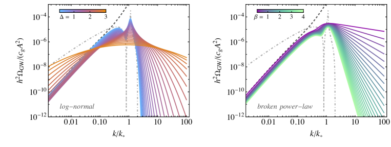
where describe respectively the growth and decay of the spectrum around the peak. One typically has Byrnes et al. (2019). The parameter characterizes the flatness of the peak. Additionally, in quasi-inflection-point models producing stellar-mass PBHs, we expect , while for curvaton models . Another broad class of spectra can be characterized by a log-normal (LN) shape
| (2) |
Such spectra appear, e.g., in a subset of hybrid inflation and curvaton models. We find, however, that our conclusions are only weakly dependent on the details of peak shape.
The present-day SIGW background emitted during radiation domination is gauge independent Inomata and Terada (2020); De Luca et al. (2020c); Yuan et al. (2020a); Domènech and Sasaki (2021) and possesses a spectrum
| (3) |
where and are the effective entropy and energy degrees of freedom (evaluated at the time of horizon crossing of mode and at present-day with the superscript ), while is the current radiation abundance. Each mode crosses the horizon at the temperature given by the relation
| (4) |
while corresponding to a current GW frequency
| (5) |
The tensor mode power spectrum is Kohri and Terada (2018); Espinosa et al. (2018)
| (6) |
where the transfer function
| (7) |
To speed up the best likelihood analysis, we assume perfect radiation domination and do not account for the variation of sound speed during the QCD era (see, for example, Hajkarim and Schaffner-Bielich (2020); Abe et al. (2021)) which also leads specific imprints in the low-frequency tail of any cosmological SGWB Franciolini et al. (2023b). On top of that, cosmic expansion may additionally be affected by unknown physics in the dark sector, which can, e.g., lead to a brief period of matter domination of kination Ferreira and Joyce (1998); Pallis (2006); Redmond et al. (2018); Co et al. (2022); Gouttenoire et al. (2021); Chang and Cui (2022). Both SIGW and PBH production can be strongly affected in such non-standard cosmologies Dalianis and Tringas (2019); Bhattacharya et al. (2020, 2021); Ireland et al. (2023); Bhattacharya (2023); Ghoshal et al. (2023).
Eq. (6) neglects possible corrections due to primordial NGs. This is typically justified because, contrary to the PBH abundance which is extremely sensitive to the tail of the distribution, the GW emission is mostly controlled by the characteristic amplitude of perturbations, and thus well captured by the leading order. In general, the computation of the SGWB is dominated by Eq. (6) and remains the in the perturbative regime if , where is the coefficient in front of the quadratic piece of the expansion (see Eq. (11) below). For the type of NGs considered in this work, we always remain within this limit. Interestingly, however, both negative and positive increase the SIGW abundance, with the next to leading order correction Cai et al. (2019); Unal (2019); Yuan and Huang (2021); Atal and Domènech (2021); Adshead et al. (2021); Abe et al. (2023); Chang et al. (2023); Garcia-Saenz et al. (2023); Li et al. (2023) (see also Bartolo et al. (2007)). We leave the inclusion of these higher-order corrections for future work.
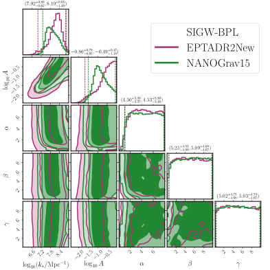
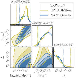
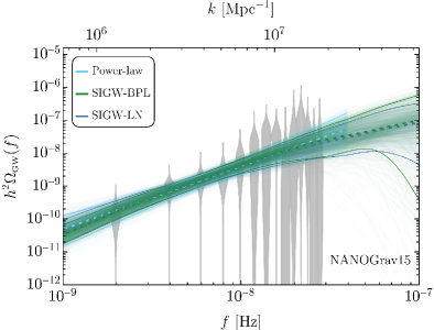
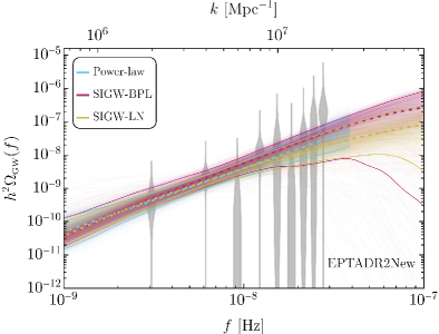
We perform a log-likelihood analysis of the NANOGrav15 and EPTA data, fitting, respectively, the posterior distributions for for the 14 frequency bins reported in Ref. Agazie et al. (2023a, b) and for the 9 frequency bin Antoniadis et al. (2023a), including only the last years of data. The results are shown in Figs. 1 and 2 for the BPL and LN scenarios, respectively. This analysis is simplified when compared to the one reported by PTA collaborations, which fit the PTA time delay data, modelling pulsar intrinsic noise as well as pulsar angular correlations. However, it provides fits consistent with the results of the NANOGrav Afzal et al. (2023) and EPTA Antoniadis et al. (2023c) collaborations and thus suffices for the purposes of this letter. We neglect potential astrophysical foregrounds, by assuming that the signal arises purely from SIGWs. Around or flat low tails, the scenarios considered here are also constrained by CMB observations Pagano et al. (2016); Chluba et al. (2012). However, these constraints tend to be less strict than PBH overproduction and we will neglect them here.
It is striking to see that the posterior distributions shown in Figs. 1 and 2 for both BPL and LN analyses indicate a rather weak dependence on the shape parameters, which are (,,) and , respectively, as long as the spectra are sufficiently narrow in the IR, i.e. and at . This is because the recent PTA data prefers blue-tilted spectra generated below frequencies of SIGW peak around .
At small scales (), the SIGW asymptotes to (for details, see the SM)
| (8) |
where and are parameters that depend mildly on the shape of the curvature power spectrum, see more details in the Supplementary material (SM). The asymptotic “causality” tail is too steep to fit the NANOGrav15 well, being disfavoured by over . However, this tension may be relieved by QCD effects Franciolini et al. (2023b). As a result, the region providing the best fit typically lies between the peak and the causality tail, at scales slightly lower than at which the spectral slope is milder. Such a milder dependence can be observed in the panel of Figs. 1 and 2, where in the region scales roughly linearly with indicating that has an approximately quadratic dependence on in the frequency range relevant PTA experiments. Additionally, since at , the peaks in the SIGW spectrum lie outside of the PTA frequency range. This can also be observed from Fig. S2.
PBH abundance – To properly compute the abundance of PBHs, two kinds of NGs need to be taken into account. Firstly, the relation between curvature and density perturbations in the long-wavelength approximation is intrinsically nonlinear Harada et al. (2015); Musco (2019)
| (9) |
where denotes the scale factor, the Hubble rate, is related to the equation of state parameter of the universe. For constant, Polnarev and Musco (2007). We have dropped the explicit and dependence or the sake of brevity.
Therefore, even for Gaussian curvature perturbations, the density fluctuations will inevitably inherit NGs from nonlinear corrections De Luca et al. (2019); Young et al. (2019); Germani and Sheth (2020). Second, there is no guarantee that is a Gaussian field – we refer to such cases as primordial NGs. The relation
| (10) |
between and its Gaussian counterpart depends on the physical mechanism that generates the enhancement of the power spectrum at small scales. These NGs are generically independent of large-scale NGs constrained by CMB data (e.g. Akrami et al. (2020)).
Often, a generic model-independent approach is to consider the quadratic template
| (11) |
with as a free parameter. However, in explicit PBH formation models, the quadratic expansion may not be sufficient. Therefore, we will also consider two specific cases of in which the primordial NG can be worked out explicitly. First, in quasi-inflection-point models of single-field inflation, the peak in arises from a brief phase of ultra-slow-roll followed by constant-roll inflation dual to it Atal and Germani (2019); Biagetti et al. (2018); Karam et al. (2023a). In this case, the NGs can be related to the large spectral slope Atal et al. (2019); Tomberg (2023),
| (12) |
Second, in curvaton models Sasaki et al. (2006); Pi and Sasaki (2023),
| (13) |
where is a function of (see Eq. (S7) in the SM for details) which we take to be the free parameter in our analysis. Curvaton self-interactions may modify the NGs (see e.g. Refs. Enqvist et al. (2010); Fonseca and Wands (2011)). We omit their contribution here and leave such investigation for future work.
We follow the prescription presented in Ref. Ferrante et al. (2023b) (see also Gow et al. (2023)) based on threshold statistics on the compaction function . The prescription improves upon the recent literature Young and Byrnes (2013); Bugaev and Klimai (2013); Young et al. (2014); Nakama et al. (2017); Byrnes et al. (2012); Franciolini et al. (2018); Yoo et al. (2018); Kawasaki and Nakatsuka (2019); Riccardi et al. (2021); Taoso and Urbano (2021); Biagetti et al. (2021); Kitajima et al. (2021); Hooshangi et al. (2022); Meng et al. (2022); Young (2022); Escrivà et al. (2022); Hooshangi et al. (2023) by both including NL and the full primordial NG functional form (10) non-perturbatively.111We mention here that slight discrepancies remain between peak theory and threshold statistics (see, e.g., Refs. Green et al. (2004); Young et al. (2014); De Luca et al. (2019)). As the former approach provides slightly smaller amplitudes, our conclusions remain conservative. The total abundance of PBHs is given by the integral (see e.g. Karam et al. (2023a))
| (14) | ||||
where is the cold dark matter density of the universe and the horizon mass corresponds to the temperature
| (15) |
We compute the mass fraction by integrating the joint probability distribution function
| (16) |
where the domain of integration is given by , and the compaction function can be built from the linear component, that uses . The Gaussian components are distributed as
| (17) |
The correlators are given by
| (18a) | |||
| (18b) | |||
| (18c) | |||
with , and . We have defined and as the top-hat window function, the spherical-shell window function, and the radiation transfer function, computed assuming radiation domination Young (2022). 222The softening of the equation of state near the QCD transitions is expected to slightly affect the evolution of sub-horizon modes. Since this is mitigated by the window function that also smooths out sub-horizon modes, we neglect this effect here.
In this work, we have followed the prescription given in Ref. Musco et al. (2021) to compute the values of the threshold and the position of the maximum of the compaction function , which depend on the shape of the power spectrum. The presence of the QCD phase transitions is taken into account by considering that and are functions of the horizon mass around Franciolini et al. (2022a); Musco et al. (2023). We give more details in the SM.
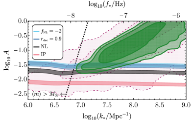
The effect of NGs is illustrated in Fig. 3 for a BPL model with , , and . We find this scenario to be one of the more conservative ones, that is, changing the shape parameters or switching to an LN shape would yield similar or less optimistic conclusions for SIGW explanations of the recent PTA data.
Fig. 3 shows that even in the absence of primordial NGs, the region avoiding overproduction of PBHs (black band and below) is excluded at over by NANOGrav15 while EPTA is currently less constraining. This conclusion confirms the results obtained in Ref. Dandoy et al. (2023) based on IPTA-DR2 data Antoniadis et al. (2022). Existing constraints on the PBH abundance force to fall at the lower edge of the colored band, and slightly strengthen this conclusion. For quasi-inflection-point models, the situation is more dire as NGs tend to assist PBH production which pushes the overproduction limit below the region for NANOGrav15. Although both the slope and the NGs in the case, shown in red, are quite large, reducing the cannot bring these models above the black band. All in all, we can conclude that constraints on the PBH abundance disfavor quasi-inflection-point models as a potential explanation for NANOGrav15. The flip-side of this conclusion is that NANOGrav15 does not impose additional constraints on the PBH abundance. Thus, a component of the signal may be related to the formation of subsolar mass PBHs that may be independently probed by future GW experiments De Luca et al. (2021b); Pujolas et al. (2021); Miller et al. (2021); Urrutia et al. (2023); Franciolini et al. (2023c).
On the other hand, the tension between SIGWs and NANOGrav15 can be alleviated in models in which NGs suppress the PBH abundance. This is demonstrated by the blue bands in Fig. 3, which correspond to curvaton models (13) with a large and for a generic quadratic ansatz (11) with a large negative . It is important to stress, that both cases displayed in Fig. 3 represent the most optimistic scenarios: increasing above would have an unnoticeable effect on and decreasing below has a positive effect on PBH formation and would shift the lines away from the best-fit region. This is because sizeable negative curvature fluctuations can still generate large fluctuations in the compaction and seed sizeable abundance (16) (see the SM for further details).
The best-fit region for NANOGrav15 lies at scales which corresponds to the production of sub-solar mass PBHs (see Fig. 3). Around , small dents in the colored bands in Fig. 3 can be observed. These arise due to the effect of the QCD phase transition which promotes PBH formation. Thus, we find that the QCD-induced enhancement of in the parameter space relevant for NANOGrav15 tends to be negligible.
Although our estimates assume quite narrow curvature power spectra, we checked that our conclusions about PBH overproduction in single-field inflation persist also in the case of broad spectra (e.g. see the models in Refs. De Luca et al. (2021a); Sugiyama et al. (2021); Franciolini and Urbano (2022); Ferrante et al. (2023a) connecting PTA observations to asteroidal mass PBH dark matter).
As a last remark, limiting our analysis to the absence of NGs in the curvature perturbation field , we have found that our results differ from those published by the NANOGrav collaboration Afzal et al. (2023). These discrepancies arise because their analysis is subject to a few simplifications: the omission of critical collapse and the nonlinear relationship between curvature perturbations and density contrast, the adoption of a different value for the threshold (independently from the curvature power spectrum), and the use of a Gaussian window function (which is incompatible with their choice of threshold Young (2019)). Another minor limitation is that they disregard any corrections from the QCD equation of state, although we find that the result is minimally dependent on this aspect.333Note added: Similar and other simplifications were made in Ref. Inomata et al. (2023); Wang et al. (2023); Liu et al. (2023) which appeared briefly after the submission of this Letter.
Conclusions and outlook – The evidence for the Hellings-Downs angular correlation reported by the NANOGrav, EPTA, PPTA, and CPTA collaborations sets an important milestone in gravitational-wave astronomy. One of the most pressing challenges to follow is to determine the nature signal: is it astrophysical or cosmological?
In this letter, we have analyzed the possibility that this signal may originate from GWs induced by high-amplitude primordial curvature perturbations. This scenario is accompanied by the production of a sizeable abundance of PBHs. Our findings demonstrate that PBH formation models that feature Gaussian primordial perturbations, or positive NGs would overproduce PBHs unless the amplitude of the spectrum is much smaller than required to explain the GW signal. For instance, most models relying on single-field inflation featuring an inflection point appear to be excluded at as the sole explanation of the NANOGrav 15-year data. However, this tension can be alleviated for models where large negative NGs suppress the PBH abundance. For instance, curvaton scenarios with a large and models exhibiting only large negative . As a byproduct, however, we conclude that the PTA data does not impose constraints on the PBH abundance.
Several future steps should be taken to improve the analysis of this paper. For instance, it would be important to fully include the impact of NGs and the variation of sound speed during the QCD era when calculating the present-day SIGW background, which provides a significant computational challenge. Beyond that, it would be important to include NGs corrections to the threshold for collapse and to reduce remaining uncertainties in the computation of the abundance. Finally, we expect that a comprehensive joint analysis involving all collaborations within the International Pulsar Timing Array (IPTA) framework will further strengthen the constraints discussed in this work.
Acknowledgements.
Acknowledgments – We thank V. De Luca, G. Ferrante, D. Racco, A. Riotto, F. Rompineve, A. Urbano, and J. Urrutia for useful discussions. G.F. acknowledges the financial support provided under the European Union’s H2020 ERC, Starting Grant agreement no. DarkGRA–757480 and under the MIUR PRIN programme, and support from the Amaldi Research Center funded by the MIUR program “Dipartimento di Eccellenza” (CUP: B81I18001170001). This work was supported by the EU Horizon 2020 Research and Innovation Programme under the Marie Sklodowska-Curie Grant Agreement No. 101007855 and additional financial support provided by “Progetti per Avvio alla Ricerca - Tipo 2”, protocol number AR2221816C515921. A.J.I. acknowledges the financial support provided under the “Progetti per Avvio alla Ricerca Tipo 1”, protocol number AR12218167D66D36, and the “Progetti di mobilità di studenti di dottorato di ricerca”. The work of V.V. and H.V. was supported by European Regional Development Fund through the CoE program grant TK133 and by the Estonian Research Council grants PRG803 and PSG869. The work of V.V. has been partially supported by the European Union’s Horizon Europe research and innovation program under the Marie Skłodowska-Curie grant agreement No. 101065736.References
- Arzoumanian et al. (2020) Z. Arzoumanian et al. (NANOGrav), Astrophys. J. Lett. 905, L34 (2020), arXiv:2009.04496 [astro-ph.HE] .
- Arzoumanian et al. (2021) Z. Arzoumanian et al. (NANOGrav), Phys. Rev. Lett. 127, 251302 (2021), arXiv:2104.13930 [astro-ph.CO] .
- Xue et al. (2021) X. Xue et al., Phys. Rev. Lett. 127, 251303 (2021), arXiv:2110.03096 [astro-ph.CO] .
- Nakai et al. (2021) Y. Nakai, M. Suzuki, F. Takahashi, and M. Yamada, Phys. Lett. B 816, 136238 (2021), arXiv:2009.09754 [astro-ph.CO] .
- Di Bari et al. (2021) P. Di Bari, D. Marfatia, and Y.-L. Zhou, JHEP 10, 193 (2021), arXiv:2106.00025 [hep-ph] .
- Sakharov et al. (2021) A. S. Sakharov, Y. N. Eroshenko, and S. G. Rubin, Phys. Rev. D 104, 043005 (2021), arXiv:2104.08750 [hep-ph] .
- Li et al. (2021) S.-L. Li, L. Shao, P. Wu, and H. Yu, Phys. Rev. D 104, 043510 (2021), arXiv:2101.08012 [astro-ph.CO] .
- Ashoorioon et al. (2022) A. Ashoorioon, K. Rezazadeh, and A. Rostami, Phys. Lett. B 835, 137542 (2022), arXiv:2202.01131 [astro-ph.CO] .
- Benetti et al. (2022) M. Benetti, L. L. Graef, and S. Vagnozzi, Phys. Rev. D 105, 043520 (2022), arXiv:2111.04758 [astro-ph.CO] .
- Barir et al. (2022) J. Barir, M. Geller, C. Sun, and T. Volansky, (2022), arXiv:2203.00693 [hep-ph] .
- Hindmarsh and Kume (2023) M. Hindmarsh and J. Kume, JCAP 04, 045 (2023), arXiv:2210.06178 [astro-ph.CO] .
- Gouttenoire and Volansky (2023) Y. Gouttenoire and T. Volansky, (2023), arXiv:2305.04942 [hep-ph] .
- Baldes et al. (2023) I. Baldes, M. Dichtl, Y. Gouttenoire, and F. Sala, (2023), arXiv:2306.15555 [hep-ph] .
- Ellis and Lewicki (2021) J. Ellis and M. Lewicki, Phys. Rev. Lett. 126, 041304 (2021), arXiv:2009.06555 [astro-ph.CO] .
- Datta et al. (2021) S. Datta, A. Ghosal, and R. Samanta, JCAP 08, 021 (2021), arXiv:2012.14981 [hep-ph] .
- Samanta and Datta (2021) R. Samanta and S. Datta, JHEP 05, 211 (2021), arXiv:2009.13452 [hep-ph] .
- Buchmuller et al. (2020) W. Buchmuller, V. Domcke, and K. Schmitz, Phys. Lett. B 811, 135914 (2020), arXiv:2009.10649 [astro-ph.CO] .
- Blasi et al. (2021) S. Blasi, V. Brdar, and K. Schmitz, Phys. Rev. Lett. 126, 041305 (2021), arXiv:2009.06607 [astro-ph.CO] .
- Gorghetto et al. (2021) M. Gorghetto, E. Hardy, and H. Nicolaescu, JCAP 06, 034 (2021), arXiv:2101.11007 [hep-ph] .
- Buchmuller et al. (2021) W. Buchmuller, V. Domcke, and K. Schmitz, JCAP 12, 006 (2021), arXiv:2107.04578 [hep-ph] .
- Blanco-Pillado et al. (2021) J. J. Blanco-Pillado, K. D. Olum, and J. M. Wachter, Phys. Rev. D 103, 103512 (2021), arXiv:2102.08194 [astro-ph.CO] .
- Ferreira et al. (2023) R. Z. Ferreira, A. Notari, O. Pujolas, and F. Rompineve, JCAP 02, 001 (2023), arXiv:2204.04228 [astro-ph.CO] .
- An and Yang (2023) H. An and C. Yang, (2023), arXiv:2304.02361 [hep-ph] .
- Qiu and Yu (2023) Z.-Y. Qiu and Z.-H. Yu, Chin. Phys. C 47, 085104 (2023), arXiv:2304.02506 [hep-ph] .
- Zeng et al. (2023) Z.-M. Zeng, J. Liu, and Z.-K. Guo, (2023), arXiv:2301.07230 [astro-ph.CO] .
- King et al. (2023) S. F. King, D. Marfatia, and M. H. Rahat, (2023), arXiv:2306.05389 [hep-ph] .
- Vaskonen and Veermäe (2021) V. Vaskonen and H. Veermäe, Phys. Rev. Lett. 126, 051303 (2021), arXiv:2009.07832 [astro-ph.CO] .
- Chen et al. (2020) Z.-C. Chen, C. Yuan, and Q.-G. Huang, Phys. Rev. Lett. 124, 251101 (2020), arXiv:1910.12239 [astro-ph.CO] .
- De Luca et al. (2021a) V. De Luca, G. Franciolini, and A. Riotto, Phys. Rev. Lett. 126, 041303 (2021a), arXiv:2009.08268 [astro-ph.CO] .
- Bhaumik and Jain (2021) N. Bhaumik and R. K. Jain, Phys. Rev. D 104, 023531 (2021), arXiv:2009.10424 [astro-ph.CO] .
- Inomata et al. (2021) K. Inomata, M. Kawasaki, K. Mukaida, and T. T. Yanagida, Phys. Rev. Lett. 126, 131301 (2021), arXiv:2011.01270 [astro-ph.CO] .
- Kohri and Terada (2021) K. Kohri and T. Terada, Phys. Lett. B 813, 136040 (2021), arXiv:2009.11853 [astro-ph.CO] .
- Domènech and Pi (2022) G. Domènech and S. Pi, Sci. China Phys. Mech. Astron. 65, 230411 (2022), arXiv:2010.03976 [astro-ph.CO] .
- Vagnozzi (2021) S. Vagnozzi, Mon. Not. Roy. Astron. Soc. 502, L11 (2021), arXiv:2009.13432 [astro-ph.CO] .
- Namba and Suzuki (2020) R. Namba and M. Suzuki, Phys. Rev. D 102, 123527 (2020), arXiv:2009.13909 [astro-ph.CO] .
- Sugiyama et al. (2021) S. Sugiyama, V. Takhistov, E. Vitagliano, A. Kusenko, M. Sasaki, and M. Takada, Phys. Lett. B 814, 136097 (2021), arXiv:2010.02189 [astro-ph.CO] .
- Zhou et al. (2020) Z. Zhou, J. Jiang, Y.-F. Cai, M. Sasaki, and S. Pi, Phys. Rev. D 102, 103527 (2020), arXiv:2010.03537 [astro-ph.CO] .
- Lin et al. (2023) J. Lin, S. Gao, Y. Gong, Y. Lu, Z. Wang, and F. Zhang, Phys. Rev. D 107, 043517 (2023), arXiv:2111.01362 [gr-qc] .
- Rezazadeh et al. (2022) K. Rezazadeh, Z. Teimoori, S. Karimi, and K. Karami, Eur. Phys. J. C 82, 758 (2022), arXiv:2110.01482 [gr-qc] .
- Kawasaki and Nakatsuka (2021) M. Kawasaki and H. Nakatsuka, JCAP 05, 023 (2021), arXiv:2101.11244 [astro-ph.CO] .
- Ahmed et al. (2022) W. Ahmed, M. Junaid, and U. Zubair, Nucl. Phys. B 984, 115968 (2022), arXiv:2109.14838 [astro-ph.CO] .
- Yi and Fei (2023) Z. Yi and Q. Fei, Eur. Phys. J. C 83, 82 (2023), arXiv:2210.03641 [astro-ph.CO] .
- Yi (2023) Z. Yi, JCAP 03, 048 (2023), arXiv:2206.01039 [gr-qc] .
- Dandoy et al. (2023) V. Dandoy, V. Domcke, and F. Rompineve, (2023), arXiv:2302.07901 [astro-ph.CO] .
- Zhao et al. (2023) J.-X. Zhao, X.-H. Liu, and N. Li, Phys. Rev. D 107, 043515 (2023), arXiv:2302.06886 [astro-ph.CO] .
- Ferrante et al. (2023a) G. Ferrante, G. Franciolini, A. Iovino, Junior., and A. Urbano, JCAP 06, 057 (2023a), arXiv:2305.13382 [astro-ph.CO] .
- Cai et al. (2023) Y. Cai, M. Zhu, and Y.-S. Piao, (2023), arXiv:2305.10933 [gr-qc] .
- Madge et al. (2023) E. Madge, E. Morgante, C. Puchades-Ibáñez, N. Ramberg, W. Ratzinger, S. Schenk, and P. Schwaller, (2023), arXiv:2306.14856 [hep-ph] .
- Goncharov et al. (2021) B. Goncharov et al., Astrophys. J. Lett. 917, L19 (2021), arXiv:2107.12112 [astro-ph.HE] .
- Chen et al. (2021) S. Chen et al. (EPTA), Mon. Not. Roy. Astron. Soc. 508, 4970 (2021), arXiv:2110.13184 [astro-ph.HE] .
- Antoniadis et al. (2022) J. Antoniadis et al., Mon. Not. Roy. Astron. Soc. 510, 4873 (2022), arXiv:2201.03980 [astro-ph.HE] .
- Agazie et al. (2023a) G. Agazie et al. (NANOGrav), Astrophys. J. Lett. 951, L8 (2023a), arXiv:2306.16213 [astro-ph.HE] .
- Agazie et al. (2023b) G. Agazie et al. (NANOGrav), Astrophys. J. Lett. 951, L9 (2023b), arXiv:2306.16217 [astro-ph.HE] .
- Antoniadis et al. (2023a) J. Antoniadis et al. (EPTA), (2023a), arXiv:2306.16214 [astro-ph.HE] .
- Antoniadis et al. (2023b) J. Antoniadis et al. (EPTA), (2023b), 10.1051/0004-6361/202346841, arXiv:2306.16224 [astro-ph.HE] .
- Antoniadis et al. (2023c) J. Antoniadis et al. (EPTA), (2023c), arXiv:2306.16227 [astro-ph.CO] .
- Reardon et al. (2023a) D. J. Reardon et al., Astrophys. J. Lett. 951, L6 (2023a), arXiv:2306.16215 [astro-ph.HE] .
- Zic et al. (2023) A. Zic et al., (2023), arXiv:2306.16230 [astro-ph.HE] .
- Reardon et al. (2023b) D. J. Reardon et al., Astrophys. J. Lett. 951, L7 (2023b), arXiv:2306.16229 [astro-ph.HE] .
- Xu et al. (2023) H. Xu et al., Res. Astron. Astrophys. 23, 075024 (2023), arXiv:2306.16216 [astro-ph.HE] .
- Agazie et al. (2023c) G. Agazie et al. (NANOGrav), Astrophys. J. Lett. 952, L37 (2023c), arXiv:2306.16220 [astro-ph.HE] .
- Afzal et al. (2023) A. Afzal et al. (NANOGrav), Astrophys. J. Lett. 951, L11 (2023), arXiv:2306.16219 [astro-ph.HE] .
- Sesana et al. (2008) A. Sesana, A. Vecchio, and C. N. Colacino, Mon. Not. Roy. Astron. Soc. 390, 192 (2008), arXiv:0804.4476 [astro-ph] .
- Kocsis and Sesana (2011) B. Kocsis and A. Sesana, Mon. Not. Roy. Astron. Soc. 411, 1467 (2011), arXiv:1002.0584 [astro-ph.CO] .
- Kelley et al. (2017) L. Z. Kelley, L. Blecha, and L. Hernquist, Mon. Not. Roy. Astron. Soc. 464, 3131 (2017), arXiv:1606.01900 [astro-ph.HE] .
- Perrodin and Sesana (2018) D. Perrodin and A. Sesana, Astrophys. Space Sci. Libr. 457, 95 (2018), arXiv:1709.02816 [astro-ph.HE] .
- Ellis et al. (2023) J. Ellis, M. Fairbairn, G. Hütsi, M. Raidal, J. Urrutia, V. Vaskonen, and H. Veermäe, Astron. Astrophys. 676, A38 (2023), arXiv:2301.13854 [astro-ph.CO] .
- Tomita (1975) K. Tomita, Prog. Theor. Phys. 54, 730 (1975).
- Matarrese et al. (1994) S. Matarrese, O. Pantano, and D. Saez, Phys. Rev. Lett. 72, 320 (1994), arXiv:astro-ph/9310036 .
- Acquaviva et al. (2003) V. Acquaviva, N. Bartolo, S. Matarrese, and A. Riotto, Nucl. Phys. B 667, 119 (2003), arXiv:astro-ph/0209156 .
- Mollerach et al. (2004) S. Mollerach, D. Harari, and S. Matarrese, Phys. Rev. D 69, 063002 (2004), arXiv:astro-ph/0310711 .
- Ananda et al. (2007) K. N. Ananda, C. Clarkson, and D. Wands, Phys. Rev. D 75, 123518 (2007), arXiv:gr-qc/0612013 .
- Baumann et al. (2007) D. Baumann, P. J. Steinhardt, K. Takahashi, and K. Ichiki, Phys. Rev. D 76, 084019 (2007), arXiv:hep-th/0703290 .
- Domènech (2021) G. Domènech, Universe 7, 398 (2021), arXiv:2109.01398 [gr-qc] .
- Carr and Hawking (1974) B. J. Carr and S. W. Hawking, Mon. Not. Roy. Astron. Soc. 168, 399 (1974).
- Carr (1975) B. J. Carr, Astrophys. J. 201, 1 (1975).
- Garcia-Bellido et al. (1996) J. Garcia-Bellido, A. D. Linde, and D. Wands, Phys. Rev. D 54, 6040 (1996), arXiv:astro-ph/9605094 .
- Ivanov et al. (1994) P. Ivanov, P. Naselsky, and I. Novikov, Phys. Rev. D 50, 7173 (1994).
- Ivanov (1998) P. Ivanov, Phys. Rev. D 57, 7145 (1998), arXiv:astro-ph/9708224 .
- Carr et al. (2021) B. Carr, K. Kohri, Y. Sendouda, and J. Yokoyama, Rept. Prog. Phys. 84, 116902 (2021), arXiv:2002.12778 [astro-ph.CO] .
- Green and Kavanagh (2021) A. M. Green and B. J. Kavanagh, J. Phys. G 48, 043001 (2021), arXiv:2007.10722 [astro-ph.CO] .
- Tisserand et al. (2007) P. Tisserand et al. (EROS-2), Astron. Astrophys. 469, 387 (2007), arXiv:astro-ph/0607207 .
- Allsman et al. (2001) R. A. Allsman et al. (Macho), Astrophys. J. Lett. 550, L169 (2001), arXiv:astro-ph/0011506 .
- Zumalacarregui and Seljak (2018) M. Zumalacarregui and U. Seljak, Phys. Rev. Lett. 121, 141101 (2018), arXiv:1712.02240 [astro-ph.CO] .
- Gorton and Green (2022) M. Gorton and A. M. Green, JCAP 08, 035 (2022), arXiv:2203.04209 [astro-ph.CO] .
- Petač et al. (2022) M. Petač, J. Lavalle, and K. Jedamzik, Phys. Rev. D 105, 083520 (2022), arXiv:2201.02521 [astro-ph.CO] .
- De Luca et al. (2022) V. De Luca, G. Franciolini, A. Riotto, and H. Veermäe, Phys. Rev. Lett. 129, 191302 (2022), arXiv:2208.01683 [astro-ph.CO] .
- Raidal et al. (2017) M. Raidal, V. Vaskonen, and H. Veermäe, JCAP 09, 037 (2017), arXiv:1707.01480 [astro-ph.CO] .
- Ali-Haïmoud et al. (2017) Y. Ali-Haïmoud, E. D. Kovetz, and M. Kamionkowski, Phys. Rev. D 96, 123523 (2017), arXiv:1709.06576 [astro-ph.CO] .
- Raidal et al. (2019) M. Raidal, C. Spethmann, V. Vaskonen, and H. Veermäe, JCAP 02, 018 (2019), arXiv:1812.01930 [astro-ph.CO] .
- Vaskonen and Veermäe (2020) V. Vaskonen and H. Veermäe, Phys. Rev. D 101, 043015 (2020), arXiv:1908.09752 [astro-ph.CO] .
- Hütsi et al. (2021) G. Hütsi, M. Raidal, V. Vaskonen, and H. Veermäe, JCAP 03, 068 (2021), arXiv:2012.02786 [astro-ph.CO] .
- Franciolini et al. (2022a) G. Franciolini, I. Musco, P. Pani, and A. Urbano, Phys. Rev. D 106, 123526 (2022a), arXiv:2209.05959 [astro-ph.CO] .
- Ricotti et al. (2008) M. Ricotti, J. P. Ostriker, and K. J. Mack, Astrophys. J. 680, 829 (2008), arXiv:0709.0524 [astro-ph] .
- Horowitz (2016) B. Horowitz, (2016), arXiv:1612.07264 [astro-ph.CO] .
- Ali-Haïmoud and Kamionkowski (2017) Y. Ali-Haïmoud and M. Kamionkowski, Phys. Rev. D 95, 043534 (2017), arXiv:1612.05644 [astro-ph.CO] .
- Poulin et al. (2017) V. Poulin, P. D. Serpico, F. Calore, S. Clesse, and K. Kohri, Phys. Rev. D 96, 083524 (2017), arXiv:1707.04206 [astro-ph.CO] .
- Hektor et al. (2018) A. Hektor, G. Hütsi, L. Marzola, M. Raidal, V. Vaskonen, and H. Veermäe, Phys. Rev. D 98, 023503 (2018), arXiv:1803.09697 [astro-ph.CO] .
- Hütsi et al. (2019) G. Hütsi, M. Raidal, and H. Veermäe, Phys. Rev. D 100, 083016 (2019), arXiv:1907.06533 [astro-ph.CO] .
- Serpico et al. (2020) P. D. Serpico, V. Poulin, D. Inman, and K. Kohri, Phys. Rev. Res. 2, 023204 (2020), arXiv:2002.10771 [astro-ph.CO] .
- De Luca et al. (2020a) V. De Luca, V. Desjacques, G. Franciolini, and A. Riotto, JCAP 11, 028 (2020a), arXiv:2009.04731 [astro-ph.CO] .
- De Luca et al. (2020b) V. De Luca, G. Franciolini, P. Pani, and A. Riotto, JCAP 06, 044 (2020b), arXiv:2005.05641 [astro-ph.CO] .
- Franciolini et al. (2022b) G. Franciolini, V. Baibhav, V. De Luca, K. K. Y. Ng, K. W. K. Wong, E. Berti, P. Pani, A. Riotto, and S. Vitale, Phys. Rev. D 105, 083526 (2022b), arXiv:2105.03349 [gr-qc] .
- Clesse and Garcia-Bellido (2022) S. Clesse and J. Garcia-Bellido, Phys. Dark Univ. 38, 101111 (2022), arXiv:2007.06481 [astro-ph.CO] .
- Ballesteros et al. (2020) G. Ballesteros, J. Rey, M. Taoso, and A. Urbano, JCAP 07, 025 (2020), arXiv:2001.08220 [astro-ph.CO] .
- Inomata et al. (2017) K. Inomata, M. Kawasaki, K. Mukaida, Y. Tada, and T. T. Yanagida, Phys. Rev. D 95, 123510 (2017), arXiv:1611.06130 [astro-ph.CO] .
- Iacconi et al. (2022) L. Iacconi, H. Assadullahi, M. Fasiello, and D. Wands, JCAP 06, 007 (2022), arXiv:2112.05092 [astro-ph.CO] .
- Kawai and Kim (2021) S. Kawai and J. Kim, Phys. Rev. D 104, 083545 (2021), arXiv:2108.01340 [astro-ph.CO] .
- Bhaumik and Jain (2020) N. Bhaumik and R. K. Jain, JCAP 01, 037 (2020), arXiv:1907.04125 [astro-ph.CO] .
- Cheong et al. (2021) D. Y. Cheong, S. M. Lee, and S. C. Park, JCAP 01, 032 (2021), arXiv:1912.12032 [hep-ph] .
- Inomata et al. (2018) K. Inomata, M. Kawasaki, K. Mukaida, and T. T. Yanagida, Phys. Rev. D 97, 043514 (2018), arXiv:1711.06129 [astro-ph.CO] .
- Dalianis et al. (2019) I. Dalianis, A. Kehagias, and G. Tringas, JCAP 01, 037 (2019), arXiv:1805.09483 [astro-ph.CO] .
- Kannike et al. (2017) K. Kannike, L. Marzola, M. Raidal, and H. Veermäe, JCAP 09, 020 (2017), arXiv:1705.06225 [astro-ph.CO] .
- Motohashi et al. (2020) H. Motohashi, S. Mukohyama, and M. Oliosi, JCAP 03, 002 (2020), arXiv:1910.13235 [gr-qc] .
- Hertzberg and Yamada (2018) M. P. Hertzberg and M. Yamada, Phys. Rev. D 97, 083509 (2018), arXiv:1712.09750 [astro-ph.CO] .
- Ballesteros and Taoso (2018) G. Ballesteros and M. Taoso, Phys. Rev. D 97, 023501 (2018), arXiv:1709.05565 [hep-ph] .
- Garcia-Bellido and Ruiz Morales (2017) J. Garcia-Bellido and E. Ruiz Morales, Phys. Dark Univ. 18, 47 (2017), arXiv:1702.03901 [astro-ph.CO] .
- Karam et al. (2023a) A. Karam, N. Koivunen, E. Tomberg, V. Vaskonen, and H. Veermäe, JCAP 03, 013 (2023a), arXiv:2205.13540 [astro-ph.CO] .
- Rasanen and Tomberg (2019) S. Rasanen and E. Tomberg, JCAP 01, 038 (2019), arXiv:1810.12608 [astro-ph.CO] .
- Balaji et al. (2022) S. Balaji, J. Silk, and Y.-P. Wu, JCAP 06, 008 (2022), arXiv:2202.00700 [astro-ph.CO] .
- Frolovsky and Ketov (2023) D. Frolovsky and S. V. Ketov, Universe 9, 294 (2023), arXiv:2304.12558 [astro-ph.CO] .
- Dimopoulos (2017) K. Dimopoulos, Phys. Lett. B 775, 262 (2017), arXiv:1707.05644 [hep-ph] .
- Germani and Prokopec (2017) C. Germani and T. Prokopec, Phys. Dark Univ. 18, 6 (2017), arXiv:1706.04226 [astro-ph.CO] .
- Choudhury and Mazumdar (2014) S. Choudhury and A. Mazumdar, Phys. Lett. B 733, 270 (2014), arXiv:1307.5119 [astro-ph.CO] .
- Ragavendra and Sriramkumar (2023) H. V. Ragavendra and L. Sriramkumar, Galaxies 11, 34 (2023), arXiv:2301.08887 [astro-ph.CO] .
- Cheng et al. (2022) S.-L. Cheng, D.-S. Lee, and K.-W. Ng, Phys. Lett. B 827, 136956 (2022), arXiv:2106.09275 [astro-ph.CO] .
- Franciolini et al. (2023a) G. Franciolini, A. Iovino, Junior., M. Taoso, and A. Urbano, (2023a), arXiv:2305.03491 [astro-ph.CO] .
- Karam et al. (2023b) A. Karam, N. Koivunen, E. Tomberg, A. Racioppi, and H. Veermäe, (2023b), arXiv:2305.09630 [astro-ph.CO] .
- Mishra et al. (2023) S. S. Mishra, E. J. Copeland, and A. M. Green, (2023), arXiv:2303.17375 [astro-ph.CO] .
- Cole et al. (2023) P. S. Cole, A. D. Gow, C. T. Byrnes, and S. P. Patil, JCAP 08, 031 (2023), arXiv:2304.01997 [astro-ph.CO] .
- Bugaev and Klimai (2012) E. Bugaev and P. Klimai, Phys. Rev. D 85, 103504 (2012), arXiv:1112.5601 [astro-ph.CO] .
- Clesse and García-Bellido (2015) S. Clesse and J. García-Bellido, Phys. Rev. D 92, 023524 (2015), arXiv:1501.07565 [astro-ph.CO] .
- Pi et al. (2018) S. Pi, Y.-l. Zhang, Q.-G. Huang, and M. Sasaki, JCAP 05, 042 (2018), arXiv:1712.09896 [astro-ph.CO] .
- Clesse et al. (2018) S. Clesse, J. García-Bellido, and S. Orani, (2018), arXiv:1812.11011 [astro-ph.CO] .
- Spanos and Stamou (2021) V. C. Spanos and I. D. Stamou, Phys. Rev. D 104, 123537 (2021), arXiv:2108.05671 [astro-ph.CO] .
- Tada and Yamada (2023a) Y. Tada and M. Yamada, Phys. Rev. D 107, 123539 (2023a), arXiv:2304.01249 [astro-ph.CO] .
- Tada and Yamada (2023b) Y. Tada and M. Yamada, (2023b), arXiv:2306.07324 [astro-ph.CO] .
- Enqvist and Sloth (2002) K. Enqvist and M. S. Sloth, Nucl. Phys. B 626, 395 (2002), arXiv:hep-ph/0109214 .
- Lyth and Wands (2002) D. H. Lyth and D. Wands, Phys. Lett. B 524, 5 (2002), arXiv:hep-ph/0110002 .
- Sloth (2003) M. S. Sloth, Nucl. Phys. B 656, 239 (2003), arXiv:hep-ph/0208241 .
- Lyth et al. (2003) D. H. Lyth, C. Ungarelli, and D. Wands, Phys. Rev. D 67, 023503 (2003), arXiv:astro-ph/0208055 .
- Dimopoulos et al. (2003) K. Dimopoulos, G. Lazarides, D. Lyth, and R. Ruiz de Austri, JHEP 05, 057 (2003), arXiv:hep-ph/0303154 .
- Kohri et al. (2013) K. Kohri, C.-M. Lin, and T. Matsuda, Phys. Rev. D 87, 103527 (2013), arXiv:1211.2371 [hep-ph] .
- Kawasaki et al. (2013a) M. Kawasaki, N. Kitajima, and T. T. Yanagida, Phys. Rev. D 87, 063519 (2013a), arXiv:1207.2550 [hep-ph] .
- Kawasaki et al. (2013b) M. Kawasaki, N. Kitajima, and S. Yokoyama, JCAP 08, 042 (2013b), arXiv:1305.4464 [astro-ph.CO] .
- Carr et al. (2017) B. Carr, T. Tenkanen, and V. Vaskonen, Phys. Rev. D 96, 063507 (2017), arXiv:1706.03746 [astro-ph.CO] .
- Ando et al. (2018a) K. Ando, K. Inomata, M. Kawasaki, K. Mukaida, and T. T. Yanagida, Phys. Rev. D 97, 123512 (2018a), arXiv:1711.08956 [astro-ph.CO] .
- Ando et al. (2018b) K. Ando, M. Kawasaki, and H. Nakatsuka, Phys. Rev. D 98, 083508 (2018b), arXiv:1805.07757 [astro-ph.CO] .
- Chen and Cai (2019) C. Chen and Y.-F. Cai, JCAP 10, 068 (2019), arXiv:1908.03942 [astro-ph.CO] .
- Liu and Prokopec (2021) L.-H. Liu and T. Prokopec, JCAP 06, 033 (2021), arXiv:2005.11069 [astro-ph.CO] .
- Pi and Sasaki (2021) S. Pi and M. Sasaki, (2021), arXiv:2112.12680 [astro-ph.CO] .
- Cai et al. (2021) R.-G. Cai, C. Chen, and C. Fu, Phys. Rev. D 104, 083537 (2021), arXiv:2108.03422 [astro-ph.CO] .
- Liu (2023) L.-H. Liu, Chin. Phys. C 47, 1 (2023), arXiv:2107.07310 [astro-ph.CO] .
- Chen et al. (2023) C. Chen, A. Ghoshal, Z. Lalak, Y. Luo, and A. Naskar, JCAP 08, 041 (2023), arXiv:2305.12325 [astro-ph.CO] .
- Torrado et al. (2018) J. Torrado, C. T. Byrnes, R. J. Hardwick, V. Vennin, and D. Wands, Phys. Rev. D 98, 063525 (2018), arXiv:1712.05364 [astro-ph.CO] .
- Cable and Wilkins (2023) A. Cable and A. Wilkins, (2023), arXiv:2306.09232 [astro-ph.CO] .
- Byrnes et al. (2019) C. T. Byrnes, P. S. Cole, and S. P. Patil, JCAP 06, 028 (2019), arXiv:1811.11158 [astro-ph.CO] .
- Inomata and Terada (2020) K. Inomata and T. Terada, Phys. Rev. D 101, 023523 (2020), arXiv:1912.00785 [gr-qc] .
- De Luca et al. (2020c) V. De Luca, G. Franciolini, A. Kehagias, and A. Riotto, JCAP 03, 014 (2020c), arXiv:1911.09689 [gr-qc] .
- Yuan et al. (2020a) C. Yuan, Z.-C. Chen, and Q.-G. Huang, Phys. Rev. D 101, 063018 (2020a), arXiv:1912.00885 [astro-ph.CO] .
- Domènech and Sasaki (2021) G. Domènech and M. Sasaki, Phys. Rev. D 103, 063531 (2021), arXiv:2012.14016 [gr-qc] .
- Kohri and Terada (2018) K. Kohri and T. Terada, Phys. Rev. D 97, 123532 (2018), arXiv:1804.08577 [gr-qc] .
- Espinosa et al. (2018) J. R. Espinosa, D. Racco, and A. Riotto, JCAP 09, 012 (2018), arXiv:1804.07732 [hep-ph] .
- Hajkarim and Schaffner-Bielich (2020) F. Hajkarim and J. Schaffner-Bielich, Phys. Rev. D 101, 043522 (2020), arXiv:1910.12357 [hep-ph] .
- Abe et al. (2021) K. T. Abe, Y. Tada, and I. Ueda, JCAP 06, 048 (2021), arXiv:2010.06193 [astro-ph.CO] .
- Franciolini et al. (2023b) G. Franciolini, D. Racco, and F. Rompineve, (2023b), arXiv:2306.17136 [astro-ph.CO] .
- Ferreira and Joyce (1998) P. G. Ferreira and M. Joyce, Phys. Rev. D 58, 023503 (1998), arXiv:astro-ph/9711102 .
- Pallis (2006) C. Pallis, Nucl. Phys. B 751, 129 (2006), arXiv:hep-ph/0510234 .
- Redmond et al. (2018) K. Redmond, A. Trezza, and A. L. Erickcek, Phys. Rev. D 98, 063504 (2018), arXiv:1807.01327 [astro-ph.CO] .
- Co et al. (2022) R. T. Co, D. Dunsky, N. Fernandez, A. Ghalsasi, L. J. Hall, K. Harigaya, and J. Shelton, JHEP 09, 116 (2022), arXiv:2108.09299 [hep-ph] .
- Gouttenoire et al. (2021) Y. Gouttenoire, G. Servant, and P. Simakachorn, (2021), arXiv:2111.01150 [hep-ph] .
- Chang and Cui (2022) C.-F. Chang and Y. Cui, JHEP 03, 114 (2022), arXiv:2106.09746 [hep-ph] .
- Dalianis and Tringas (2019) I. Dalianis and G. Tringas, Phys. Rev. D 100, 083512 (2019), arXiv:1905.01741 [astro-ph.CO] .
- Bhattacharya et al. (2020) S. Bhattacharya, S. Mohanty, and P. Parashari, Phys. Rev. D 102, 043522 (2020), arXiv:1912.01653 [astro-ph.CO] .
- Bhattacharya et al. (2021) S. Bhattacharya, S. Mohanty, and P. Parashari, Phys. Rev. D 103, 063532 (2021), arXiv:2010.05071 [astro-ph.CO] .
- Ireland et al. (2023) A. Ireland, S. Profumo, and J. Scharnhorst, Phys. Rev. D 107, 104021 (2023), arXiv:2302.10188 [gr-qc] .
- Bhattacharya (2023) S. Bhattacharya, Galaxies 11, 35 (2023), arXiv:2302.12690 [astro-ph.CO] .
- Ghoshal et al. (2023) A. Ghoshal, Y. Gouttenoire, L. Heurtier, and P. Simakachorn, (2023), arXiv:2304.04793 [hep-ph] .
- Cai et al. (2019) R.-g. Cai, S. Pi, and M. Sasaki, Phys. Rev. Lett. 122, 201101 (2019), arXiv:1810.11000 [astro-ph.CO] .
- Unal (2019) C. Unal, Phys. Rev. D 99, 041301 (2019), arXiv:1811.09151 [astro-ph.CO] .
- Yuan and Huang (2021) C. Yuan and Q.-G. Huang, Phys. Lett. B 821, 136606 (2021), arXiv:2007.10686 [astro-ph.CO] .
- Atal and Domènech (2021) V. Atal and G. Domènech, JCAP 06, 001 (2021), arXiv:2103.01056 [astro-ph.CO] .
- Adshead et al. (2021) P. Adshead, K. D. Lozanov, and Z. J. Weiner, JCAP 10, 080 (2021), arXiv:2105.01659 [astro-ph.CO] .
- Abe et al. (2023) K. T. Abe, R. Inui, Y. Tada, and S. Yokoyama, JCAP 05, 044 (2023), arXiv:2209.13891 [astro-ph.CO] .
- Chang et al. (2023) Z. Chang, Y.-T. Kuang, X. Zhang, and J.-Z. Zhou, Chin. Phys. C 47, 055104 (2023), arXiv:2209.12404 [astro-ph.CO] .
- Garcia-Saenz et al. (2023) S. Garcia-Saenz, L. Pinol, S. Renaux-Petel, and D. Werth, JCAP 03, 057 (2023), arXiv:2207.14267 [astro-ph.CO] .
- Li et al. (2023) J.-P. Li, S. Wang, Z.-C. Zhao, and K. Kohri, (2023), arXiv:2305.19950 [astro-ph.CO] .
- Bartolo et al. (2007) N. Bartolo, S. Matarrese, A. Riotto, and A. Vaihkonen, Phys. Rev. D 76, 061302 (2007), arXiv:0705.4240 [astro-ph] .
- Pagano et al. (2016) L. Pagano, L. Salvati, and A. Melchiorri, Phys. Lett. B 760, 823 (2016), arXiv:1508.02393 [astro-ph.CO] .
- Chluba et al. (2012) J. Chluba, A. L. Erickcek, and I. Ben-Dayan, Astrophys. J. 758, 76 (2012), arXiv:1203.2681 [astro-ph.CO] .
- Harada et al. (2015) T. Harada, C.-M. Yoo, T. Nakama, and Y. Koga, Phys. Rev. D 91, 084057 (2015), arXiv:1503.03934 [gr-qc] .
- Musco (2019) I. Musco, Phys. Rev. D 100, 123524 (2019), arXiv:1809.02127 [gr-qc] .
- Polnarev and Musco (2007) A. G. Polnarev and I. Musco, Class. Quant. Grav. 24, 1405 (2007), arXiv:gr-qc/0605122 .
- De Luca et al. (2019) V. De Luca, G. Franciolini, A. Kehagias, M. Peloso, A. Riotto, and C. Ünal, JCAP 07, 048 (2019), arXiv:1904.00970 [astro-ph.CO] .
- Young et al. (2019) S. Young, I. Musco, and C. T. Byrnes, JCAP 11, 012 (2019), arXiv:1904.00984 [astro-ph.CO] .
- Germani and Sheth (2020) C. Germani and R. K. Sheth, Phys. Rev. D 101, 063520 (2020), arXiv:1912.07072 [astro-ph.CO] .
- Akrami et al. (2020) Y. Akrami et al. (Planck), Astron. Astrophys. 641, A9 (2020), arXiv:1905.05697 [astro-ph.CO] .
- Atal and Germani (2019) V. Atal and C. Germani, Phys. Dark Univ. 24, 100275 (2019), arXiv:1811.07857 [astro-ph.CO] .
- Biagetti et al. (2018) M. Biagetti, G. Franciolini, A. Kehagias, and A. Riotto, JCAP 07, 032 (2018), arXiv:1804.07124 [astro-ph.CO] .
- Atal et al. (2019) V. Atal, J. Garriga, and A. Marcos-Caballero, JCAP 09, 073 (2019), arXiv:1905.13202 [astro-ph.CO] .
- Tomberg (2023) E. Tomberg, Phys. Rev. D 108, 043502 (2023), arXiv:2304.10903 [astro-ph.CO] .
- Sasaki et al. (2006) M. Sasaki, J. Valiviita, and D. Wands, Phys. Rev. D 74, 103003 (2006), arXiv:astro-ph/0607627 .
- Pi and Sasaki (2023) S. Pi and M. Sasaki, Phys. Rev. Lett. 131, 011002 (2023), arXiv:2211.13932 [astro-ph.CO] .
- Enqvist et al. (2010) K. Enqvist, S. Nurmi, O. Taanila, and T. Takahashi, JCAP 04, 009 (2010), arXiv:0912.4657 [astro-ph.CO] .
- Fonseca and Wands (2011) J. Fonseca and D. Wands, Phys. Rev. D 83, 064025 (2011), arXiv:1101.1254 [astro-ph.CO] .
- Ferrante et al. (2023b) G. Ferrante, G. Franciolini, A. Iovino, Junior., and A. Urbano, Phys. Rev. D 107, 043520 (2023b), arXiv:2211.01728 [astro-ph.CO] .
- Gow et al. (2023) A. D. Gow, H. Assadullahi, J. H. P. Jackson, K. Koyama, V. Vennin, and D. Wands, EPL 142, 49001 (2023), arXiv:2211.08348 [astro-ph.CO] .
- Young and Byrnes (2013) S. Young and C. T. Byrnes, JCAP 08, 052 (2013), arXiv:1307.4995 [astro-ph.CO] .
- Bugaev and Klimai (2013) E. V. Bugaev and P. A. Klimai, Int. J. Mod. Phys. D 22, 1350034 (2013), arXiv:1303.3146 [astro-ph.CO] .
- Young et al. (2014) S. Young, C. T. Byrnes, and M. Sasaki, JCAP 07, 045 (2014), arXiv:1405.7023 [gr-qc] .
- Nakama et al. (2017) T. Nakama, J. Silk, and M. Kamionkowski, Phys. Rev. D 95, 043511 (2017), arXiv:1612.06264 [astro-ph.CO] .
- Byrnes et al. (2012) C. T. Byrnes, E. J. Copeland, and A. M. Green, Phys. Rev. D 86, 043512 (2012), arXiv:1206.4188 [astro-ph.CO] .
- Franciolini et al. (2018) G. Franciolini, A. Kehagias, S. Matarrese, and A. Riotto, JCAP 03, 016 (2018), arXiv:1801.09415 [astro-ph.CO] .
- Yoo et al. (2018) C.-M. Yoo, T. Harada, J. Garriga, and K. Kohri, PTEP 2018, 123E01 (2018), arXiv:1805.03946 [astro-ph.CO] .
- Kawasaki and Nakatsuka (2019) M. Kawasaki and H. Nakatsuka, Phys. Rev. D 99, 123501 (2019), arXiv:1903.02994 [astro-ph.CO] .
- Riccardi et al. (2021) F. Riccardi, M. Taoso, and A. Urbano, JCAP 08, 060 (2021), arXiv:2102.04084 [astro-ph.CO] .
- Taoso and Urbano (2021) M. Taoso and A. Urbano, JCAP 08, 016 (2021), arXiv:2102.03610 [astro-ph.CO] .
- Biagetti et al. (2021) M. Biagetti, V. De Luca, G. Franciolini, A. Kehagias, and A. Riotto, Phys. Lett. B 820, 136602 (2021), arXiv:2105.07810 [astro-ph.CO] .
- Kitajima et al. (2021) N. Kitajima, Y. Tada, S. Yokoyama, and C.-M. Yoo, JCAP 10, 053 (2021), arXiv:2109.00791 [astro-ph.CO] .
- Hooshangi et al. (2022) S. Hooshangi, M. H. Namjoo, and M. Noorbala, Phys. Lett. B 834, 137400 (2022), arXiv:2112.04520 [astro-ph.CO] .
- Meng et al. (2022) D.-S. Meng, C. Yuan, and Q.-g. Huang, Phys. Rev. D 106, 063508 (2022), arXiv:2207.07668 [astro-ph.CO] .
- Young (2022) S. Young, JCAP 05, 037 (2022), arXiv:2201.13345 [astro-ph.CO] .
- Escrivà et al. (2022) A. Escrivà, Y. Tada, S. Yokoyama, and C.-M. Yoo, JCAP 05, 012 (2022), arXiv:2202.01028 [astro-ph.CO] .
- Hooshangi et al. (2023) S. Hooshangi, M. H. Namjoo, and M. Noorbala, (2023), arXiv:2305.19257 [astro-ph.CO] .
- Green et al. (2004) A. M. Green, A. R. Liddle, K. A. Malik, and M. Sasaki, Phys. Rev. D 70, 041502 (2004), arXiv:astro-ph/0403181 .
- Musco et al. (2021) I. Musco, V. De Luca, G. Franciolini, and A. Riotto, Phys. Rev. D 103, 063538 (2021), arXiv:2011.03014 [astro-ph.CO] .
- Musco et al. (2023) I. Musco, K. Jedamzik, and S. Young, (2023), arXiv:2303.07980 [astro-ph.CO] .
- De Luca et al. (2021b) V. De Luca, G. Franciolini, P. Pani, and A. Riotto, JCAP 11, 039 (2021b), arXiv:2106.13769 [astro-ph.CO] .
- Pujolas et al. (2021) O. Pujolas, V. Vaskonen, and H. Veermäe, Phys. Rev. D 104, 083521 (2021), arXiv:2107.03379 [astro-ph.CO] .
- Miller et al. (2021) A. L. Miller, S. Clesse, F. De Lillo, G. Bruno, A. Depasse, and A. Tanasijczuk, Phys. Dark Univ. 32, 100836 (2021), arXiv:2012.12983 [astro-ph.HE] .
- Urrutia et al. (2023) J. Urrutia, V. Vaskonen, and H. Veermäe, Phys. Rev. D 108, 023507 (2023), arXiv:2303.17601 [astro-ph.CO] .
- Franciolini et al. (2023c) G. Franciolini, F. Iacovelli, M. Mancarella, M. Maggiore, P. Pani, and A. Riotto, Phys. Rev. D 108, 043506 (2023c), arXiv:2304.03160 [gr-qc] .
- Franciolini and Urbano (2022) G. Franciolini and A. Urbano, Phys. Rev. D 106, 123519 (2022), arXiv:2207.10056 [astro-ph.CO] .
- Young (2019) S. Young, Int. J. Mod. Phys. D 29, 2030002 (2019), arXiv:1905.01230 [astro-ph.CO] .
- Inomata et al. (2023) K. Inomata, K. Kohri, and T. Terada, (2023), arXiv:2306.17834 [astro-ph.CO] .
- Wang et al. (2023) S. Wang, Z.-C. Zhao, J.-P. Li, and Q.-H. Zhu, (2023), arXiv:2307.00572 [astro-ph.CO] .
- Liu et al. (2023) L. Liu, Z.-C. Chen, and Q.-G. Huang, (2023), arXiv:2307.01102 [astro-ph.CO] .
- Pi and Sasaki (2020) S. Pi and M. Sasaki, JCAP 09, 037 (2020), arXiv:2005.12306 [gr-qc] .
- Yuan et al. (2020b) C. Yuan, Z.-C. Chen, and Q.-G. Huang, Phys. Rev. D 101, 043019 (2020b), arXiv:1910.09099 [astro-ph.CO] .
- Germani and Musco (2019) C. Germani and I. Musco, Phys. Rev. Lett. 122, 141302 (2019), arXiv:1805.04087 [astro-ph.CO] .
- Escrivà et al. (2020) A. Escrivà, C. Germani, and R. K. Sheth, Phys. Rev. D 101, 044022 (2020), arXiv:1907.13311 [gr-qc] .
- Kehagias et al. (2019) A. Kehagias, I. Musco, and A. Riotto, JCAP 12, 029 (2019), arXiv:1906.07135 [astro-ph.CO] .
- Jedamzik (1998) K. Jedamzik, Phys. Rept. 307, 155 (1998), arXiv:astro-ph/9805147 .
- Byrnes et al. (2018) C. T. Byrnes, M. Hindmarsh, S. Young, and M. R. S. Hawkins, JCAP 08, 041 (2018), arXiv:1801.06138 [astro-ph.CO] .
- Escrivà et al. (2023) A. Escrivà, E. Bagui, and S. Clesse, JCAP 05, 004 (2023), arXiv:2209.06196 [astro-ph.CO] .
The recent gravitational wave observation by pulsar timing arrays
and primordial black holes: the importance of non-Gaussianities
Gabriele Franciolini, Antonio Junior Iovino, Ville Vaskonen, and Hardi Veermäe
Supplementary Material
I Asymptotics of the GW power spectrum
We report here some analytic expressions for the low asymptotics of GW spectra generated by an enhanced feature in the curvature fluctuations with BPL and LN shapes, i.e. Eqs. (1) and (2) respectively (see also Refs. Pi and Sasaki (2020); Yuan et al. (2020b)). The corresponding SIGW spectra are shown in Fig. S1. Sufficiently far away from the peak, we can drop the dependence inside and expand the transfer functions in Eq. (6)
| (S1) |
where and are parameters that depend on the shape of the curvature power spectrum and . For the power spectra (1) and (2), the asymptotics can be obtained explicitly
| (S2) | ||||
where , and denotes the polygamma function. This tail fits the numerically evaluated SIGW tails well, as can be seen in Fig. S1.
At the tail, the SIGW spectrum tracks roughly when it is sufficiently wide, that is, wider than the SIGW spectrum corresponding to the monochromatic curvature spectrum.
In Fig. S2, we show the best fit SGWB spectra for both the BPL and LN models compared to the NANOGrav15 (left panel) and EPTA (right panel) datasets.
II Dependency of the PBH formation parameters on the curvature power spectral shape
The density contrast field averaged over a spherical region of areal radius , and the compaction function , defined as twice the local mass excess over the areal radius and evaluated at the scale at which it is maximized, are related by
| (S3) |
As discussed in Ref. Musco (2019) and Refs. therein, the gravitational collapse that triggers the formation of a PBH takes place when the maximum of the compaction function is larger than a certain threshold value. Using Eq. (S3), we can relate threshold values in the compaction to the threshold for the density contrast .
In full generality, the threshold (or ) depends on the shape of the collapsing overdensities, which is controlled by the curvature power spectrum Germani and Musco (2019); Musco (2019); Musco et al. (2021). In this work, we follow Ref. Musco et al. (2021), where a prescription of how to compute the collapse parameter as a function of the curvature spectrum is derived. For completeness, we briefly report here the main steps to compute the threshold and the shape parameter . First of all, the maximum of the compaction function is located the the radius , which can be found solving numerically the integral equation
| (S4) |
Consequently, the shape parameter is obtained using
| (S5) |
where we introduced to shorten the notation. Finally, once we determined shape parameter , we can compute the threshold using the relation Escrivà et al. (2020)
| (S6) |
In Fig. S3 we show how the threshold and the shape parameter change respect the shape of the power spectrum for a BPL (right panel) and a LN (left panel).
 
|
It is worth emphasizing a general trend. As the spectrum becomes narrower, the threshold for collapse rises up to larger values. This is because, for broader spectra, more modes participate in the evolution of the collapsing overdensity, leading to a reduction of pressure gradients that facilitates the PBH formation, see Ref. Musco et al. (2021) for more details. It is important to note that the prescription outlined in Ref. Musco et al. (2021) to compute the threshold for PBH collapse only accounts for NGs arising from the non-linear relation between the density contrast and the curvature perturbations. In principle, also primordial NGs beyond the quadratic approximation should be taken into account when computing the threshold value. Following Refs. Kehagias et al. (2019); Escrivà et al. (2022), it appears that the effect on the threshold is small and at most of the order of a few percent. Interestingly, it follows the same impact NGs have on the statistics, i.e. negative (positive) NGs would tend to increase (decrease) the required amplitude of spectra. Therefore, neglecting this effect we are conservative. We left the inclusion of this effect for future work.
Due to a softening of the equation of state, the formation of PBH becomes more efficient during the QCD transition Jedamzik (1998); Byrnes et al. (2018); Franciolini et al. (2022a); Escrivà et al. (2023); Musco et al. (2023). Consequently, the formation parameters change due to the softening of the equation of state. In our analysis presented in the main text, we computed for each power spectrum, and used the results obtained in Ref.Musco et al. (2023), where the formation parameters and (or equivalently ) are obtained a function of .
III Primordial non-Gaussianities
In this section, we discuss a few relevant details about the NG models considered in this work. We summarise the behaviour of the amplitude required to produce depending on the various types of NGs discussed in this paper in Fig. S4, assuming a reference BPL power spectrum.


III.0.1 Quasi-inflection point
As described already in the main text, when presenting results inspired by the quasi-inflection point, the NG parameter is inherently determined by the UV slope of the power spectrum. As we can see from the left panel in Fig. S4, when one shrinks the shape of the power spectrum and keeps the threshold for collapse constant, we find that the amplitude should decrease to obtain . This is because NGs become larger with increasing in such models.
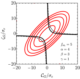
III.0.2 Quadratic non-Gaussianities
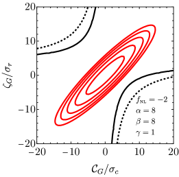
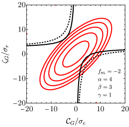
Generically, one might mistakenly assume that by pushing the coefficient towards larger negative values, the required value of the power spectral amplitude associated with would subsequently rise. As we show in the middle plot of Fig. S4, however, a maximum amplitude is reached for . The reason for the appearance of such a peak and the subsequent decrease of A for can be understood as follows. When is negative, one can still push the compaction function beyond the threshold, provided and had opposite signs or one has small and positive . In Fig. S5, we show the probability distribution for both Gaussian parameters and (red contours), compared to the overthreshold condition (between the black lines). For realistic spectra, one always finds sufficient support of the PDF in the anti-correlated direction, and thus obtain a sizeable PBH abundance. Only in the limit of a very narrow power spectrum, one finds converging towards unity, which means a perfect correlation between and , that leads to very small overlap with the parameter space producing overthreshold perturbation of the compaction function. This explains the appearance of a sharp rise of in the results Ref. Young (2022) (see their Fig. 2), which, is however, expected only for extremely narrow spectra.
For this ansatz and with , we find that the amplitude of the power spectrum saturating the abundance of PBH is around , so we should expect a correction to the SIGW spectrum of the order . Still, this is subdominant compared to the leading order term used in this paper.
III.0.3 Curvaton models
When presenting results inspired by the curvaton model, we will focus on primordial NG (derived analytically within the sudden-decay approximation Sasaki et al. (2006))
| (S7) |
with
| (S8a) | ||||
| (S8b) | ||||
| (S8c) | ||||
| (S8d) | ||||
The parameter is the weighted fraction of the curvaton energy density to the total energy density at the time of curvaton decay, defined by
| (S9) |
where is the energy density stored in radiation after reheating. Thus, depends on the physical assumptions about the physics of the curvaton within a given model.
For comparison, the coefficients in the series expansion are given by
| (S10) |
At , the fluctuations arise from the curvaton field only, as it completely dominates the energy density budget at the time of decay. This gives and , . Note that this mimics NG in inflection point models (12) with an unphysical . For the benchmark case we used in the main text, , one finds , . Also, we determine that the order of magnitude of the NG correction to the SIGW should be of order , and we do not expect any relevant correction from higher order terms in Eq. (6).