Primordial magnetic field as a common solution of nanohertz gravitational waves and Hubble tension

Abstract

The origin of interstellar and intergalactic magnetic fields remains largely unknown. One possibility is that they are related to the primordial magnetic fields (PMFs) produced by, for instance, the phase transitions of the early Universe. In this letter, we show that the PMF-induced turbulence generated at around the QCD phase transition epoch—the characteristic magnetic field strength $B_{\rm ch}^{*}\sim\mathcal{O}(1)~{}\rm{\mu G}$ and coherent length scale $\ell_{\rm ch}^{*}\sim\mathcal{O}(1)~{}\rm{pc}$, can naturally accommodate with nanohertz gravitational waves reported by pulsar timing array collaborations. Moreover, the evolution of the PMFs to the recombination era with the form of $B_{\rm ch}\sim\ell_{\rm ch}^{-\alpha}$ can induce baryon density inhomogeneities, alter the recombination history, and alleviate the tension of the Hubble parameter $H_{0}$ and the matter clumpiness parameter $S_{8}$ between early and late-time measurements for $0.88\leq\alpha\leq 1.17$ (approximate 95% credible region based on three PTA likelihoods). The further evolved PMFs may account for the $\sim{\cal O}(10^{-16})$ Gauss extra-galactic magnetic field inferred with GRB 221009A.

Introduction. A signal of stochastic gravitational wave background (SGWB) with frequencies around nanohertz (nHz) is a powerful probe of several astrophysical and physical problems Lasky:2015lej . In recent years, several pulsar timing arrays (PTAs) reported the positive detection of candidate power-law signals in the data NANOGrav:2020bcs ; Goncharov:2021oub ; Chen:2021rqp ; Antoniadis:2022pcn . Very recently, the analyses of the Hellings-Downs (HD) correlation Hellings:1983fr of the timing residuals give evidence in support of the SGWB nature of the power-law excess NANOGrav:2023gor ; Antoniadis:2023ott ; Reardon:2023gzh ; Xu:2023wog . The significance of the HD correlation obtained from NANOGrav, EPTA, PPTA, and CPTA is approximately $3\sigma$, $3\sigma$, $2\sigma$, and $4.6\sigma$, respectively. The fitted power law parameters, i.e., the amplitude and spectral index, are $A_{\rm GWB}=6.4^{+4.2}_{-2.7}\times 10^{-15}$ and $\gamma=3.2^{+0.6}_{-0.6}$ for NANOGrav, $\log_{10}A_{\rm GWB}=-14.54^{+0.28}_{-0.41}$ and $\gamma=4.19^{+0.73}_{-0.63}$ for EPTA, $A_{\rm GWB}=3.1^{+1.3}_{-0.9}\times 10^{-15}$ and $\alpha=-0.45^{+0.20}_{-0.20}$ ($\alpha=\frac{3-\gamma}{2}$) for PPTA, and $\log_{10}A_{\rm GWB}=-14.4^{+1.0}_{-2.8}$ with $\gamma<6.6$ for CPTA. These results represent the breakthrough opening a new window for observing the Universe with gravitational waves (GWs).

Besides the astrophysical origin of the SGWB from the orbital motions of supermassive binary black holes Rajagopal:1994zj ; Jaffe:2002rt ; Wyithe:2002ep ; Sesana:2004sp , it is of great interests in possible connection with many new physics processes in the early Universe, such as inflation Grishchuk:2005qe ; Vagnozzi:2020gtf ; Benetti:2021uea ; Vagnozzi:2023lwo ; Ashoorioon:2022raz , phase transitions Mazumdar:2018dfl ; Addazi:2020zcj ; NANOGrav:2021flc ; Xue:2021gyq ; Kobakhidze:2017mru ; Athron:2023xlk , cosmic strings Blasi:2020mfx ; Ellis:2020ena ; Lazarides:2021uxv ; Buchmuller:2020lbh ; Chang:2021afa ; Bian:2022tju ; EPTA:2023hof ; Samanta:2020cdk ; Datta:2020bht , domain walls Liu:2020mru ; Bian:2022qbh , or primordial black holes Vaskonen:2020lbd ; DeLuca:2020agl ; Kohri:2020qqd ; Domenech:2020ers ; Papanikolaou:2023cku ; Chen:2019xse . It has been proposed that magnetohydrodynamic (MHD) turbulence generated by the PMFs can also produce the SGWB Caprini:2001nb ; Caprini:2006jb ; RoperPol:2022iel ; Auclair:2022jod . If the PMFs were initially produced via, e.g., the QCD phase transition, the induced SGWB would fall within the detectable range of PTAs. The corresponding comoving length is about 1 pc, inversely proportional to the temperature around $100~{}\,\mathrm{MeV}$. As the Universe evolves to the recombination epoch, the PMFs can induce baryon density fluctuations. These baryon density inhomogeneities alter the standard cosmological evolution by affecting the recombination history. Consequently, it may affect the Hubble constant $H_{0}$ and the matter clumpiness parameter $S_{8}$ inferred from the cosmic microwave background (CMB) data Planck:2018vyg . As a result, it may solve or alleviate Jedamzik:2020krr ; Jedamzik:2018itu the tension from late-time measurements (e.g., Riess:2021jrx ; Reid:2019tiq ; Wong:2019kwg ).

In light of the first detection of SGWB from the PTAs, we study the PMF scenario with the purpose to account for the nHz SGWB and to alleviate the $H_{0}$ and $S_{8}$ tension simultaneously . We assume an evolutionary relation of $B_{\rm ch}\sim\ell_{\rm ch}^{-\alpha}$, where $B_{\rm ch}$ is the comoving characteristic magnetic field strength and $\ell_{\rm ch}$ is the comoving scale, to bridge the early time when PMFs were produced and the recombination epoch. The SGWB data are used to constrain the initial parameters of the PMFs. They are then implemented as a likelihood to perform a Bayesian global analysis, together with the cosmological likelihoods including the PLANCK CMB anisotropies Planck:2018vyg , the baryon acoustic oscillation (BAO; BOSS:2016wmc ; Beutler:2011hx ; Ross:2014qpa ), and the local measurements of the Hubble constant (hereafter H3) Riess:2021jrx ; Reid:2019tiq ; Wong:2019kwg . As will be shown in detail later, we find that the PMFs model can solve these two important problems simultaneously. If this is the case, we also, for the first time, obtain the evolution properties of the PMFs at different epochs of the early Universe.

SGWB from PMFs.

Figure 1: Left: The free-spectrum analysis for the NANOGrav 15-year dataset (red), PPTA DR3 (green), and EPTA DR2full (blue) and the theoretical SGWB spectra with the best-fit values of PMFs parameters. Right: The favored $68\%$ (inner) and $95\%$ (outer) parameter regions projected on the ($\log_{10}\ell_{\rm ch}^{*}$, $\log_{10}B_{\rm ch}^{*}$) plane. Those contours are obtained by fitting the timing residual signals of NANOGrav 15-year data (red), PPTA DR3 (green), and EPTA DR2full (blue). The two dashed lines are the upper limits on the total normalized magnetic energy density from the big bang nucleosynthesis constraints ($\Omega_{\rm M}^{*}=0.1$; Grasso:1996kk ; Kahniashvili:2009qi ) and the total energy density of the Universe at the initial time ($\Omega_{\rm M}^{*}=1$).

The PMF is treated as a Gaussian random field with a spectrum described by the same method as RoperPol:2022iel ; Auclair:2022jod . The spectrum of the GWs produced from the initial time $\tau_{*}$ to the end time $\tau_{\rm end}$  at the scale $k$ can be written as RoperPol:2022iel

$$\Omega_{\rm GW}(k,\tau_{\text{end}})\simeq 3\left(\frac{k}{k_{\rm ch}^{*}}\right)\Omega_{\rm M}^{*}\frac{\mathcal{C}(\alpha)}{\mathcal{A}^{2}(\alpha)}p_{\Pi}\left(\frac{k}{k_{\rm ch}^{*}}\right)$$

$$\times\bigg{\{}\begin{array}[]{lr}\ln^{2}(1+\mathcal{H}_{*}\delta\tau_{\text{end}}),&\text{if }k\,\delta\tau_{\text{end}}<1\\ \ln^{2}(1+\mathcal{H_{*}}/k),&\text{if }k\,\delta\tau_{\text{end}}\geq 1\end{array},$$ (3)

where $\Omega_{\rm M}^{*}=\frac{1}{2}(B_{\rm ch}^{*})^{2}$ is the total normalized magnetic engergy density and $k_{\rm ch}^{*}=2\pi/l_{\rm ch}^{*}$. The comoving Hubble frequency $\mathcal{H_{*}}\simeq 1.12\times 10^{-8}(T_{*}/100~{}\rm{MeV})$, where $T_{*}$ and $g_{*}$ refer to the temperature and the relativistic degrees of freedom during the QCD phase transition epoch. We set $T_{*}=$100 MeV and $g_{*}=10$ in this work. Two constants $\mathcal{C}(\alpha)$ and $\mathcal{A}(\alpha)$ have been calculated in paper RoperPol:2022iel . Also, $\delta\tau_{\rm end}=\tau_{\rm end}-\tau_{*}$ is the duration of the GW source. From the MHD simulation RoperPol:2022iel , we have $\delta\tau_{\rm end}=0.184\mathcal{H_{*}}^{-1}+1.937\delta\tau_{\rm e}$, where $\delta\tau_{\rm e}=(\sqrt{1.5\Omega_{M}^{*}}k_{ch}^{*})^{-1}$ is the eddy turn over time. The parameter $p_{\Pi}\left(k/k_{\rm ch}^{*}\right)$ is defined as $P_{\Pi}^{*}(k)/P_{\Pi}^{*}(0)$, where $P_{\Pi}^{*}(k)$ is the anisotropic stress power spectral density.

After $\tau_{\rm end}$, the sources stop acting, and the GWs start to propagate through the Universe freely while the energy density decreases due to cosmic expansion. Therefore, we have the GW today RoperPol:2022iel

$$\begin{gathered}h^{2}\Omega_{\mathrm{GW}}^{0}(k)=\left(\frac{a_{\mathrm{end}}}{a_{0}}\right)^{4}\left(\frac{H_{\mathrm{end}}}{H_{0}}\right)^{2}h^{2}\Omega_{\mathrm{GW}}\left(k,\tau_{\mathrm{end}}\right)\\ \quad\simeq 3.5\times 10^{-5}~{}\Omega_{\mathrm{GW}}\left(k,\tau_{\mathrm{end}}\right)\left(\frac{10}{g_{\mathrm{end}}}\right)^{\frac{1}{3}},\end{gathered}$$ (4)

where $a_{\rm end}$ and $a_{0}$ correspond to the scale factors. The Hubble constant $H_{\rm end}$ has been calculated in Ref. Kolb:1990vq , and $H_{0}=100h~{}\rm{kms^{-1}~{}Mpc^{-1}}$ with $h\simeq 0.68$ Planck:2018vyg . The entropic degrees of freedom $g_{\rm end}$ equals $g_{*}$. The SGWB spectrum, denoted as $h^{2}\Omega_{\rm GW}^{0}(f)$ with frequency $f$, can be linked to the timing residuals $\rho(f)$ that are directly measured by PTA experimentsNANOGRAV:2018hou .

$$\rho(f)=\frac{1}{4\pi^{2}f_{\rm yr}}\left(\frac{f}{f_{\rm yr}}\right)^{-3/2}h_{\rm c}(f),$$ (5)

$$h_{\rm c}(f)=\frac{H_{0}}{\pi f}\sqrt{\frac{3}{2}h^{2}\Omega_{\rm GW}^{0}(f)}.$$ (6)

where $f_{\rm yr}\simeq 3.17\times 10^{-8}{\rm Hz}$.

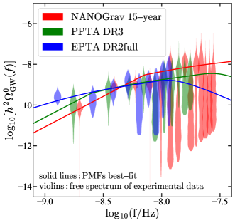
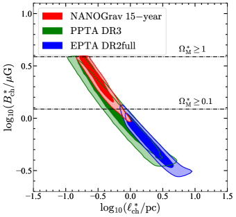
A maximum likelihood estimation method is utilized to fit the parameters of the PMF model, characteristic magnetic field strength $B_{\rm ch}^{*}$, and scale $\ell_{\rm ch}^{*}$, by means of comparing the theoretical SGWB to the common-noise free spectrum derived from PPTA DR3, EPTA DR2full, and NANOGrav 15-year data NANOGrav:2023gor ; Antoniadis:2023ott ; Reardon:2023gzh . The violin plots in the left panel of Fig. 1 depict the free spectra with Helling-Downs cross-correlations and the solid lines are the analytical SGWB spectra incorporating the best-fit values of $B_{\rm ch}^{*}$ and $\ell_{\rm ch}^{*}$. Distinct colors signify the utilization of different PTA datasets. The red, green, and blue contours in the right panel of Fig. 1 correspond to the obtained 68% and 95% confidence level parameter regions of $B_{\rm ch}^{*}$ and $l_{\rm ch}^{*}$ using the NANOGrav 15-year data, PPTA DR3, and EPTA DR2full, respectively. As shown in this panel, the favored parameters are $B_{\rm ch}^{*}\sim\mathcal{O}(1)~{}\rm{\mu G}$ and $l_{\rm ch}^{*}\sim\mathcal{O}(1)~{}\rm{pc}$. We would note that the three contours are located at slightly different regions because the amplitudes of the free spectra measured by those three experiments are different.

Baryon Inhomogeneities Induced from PMFs at Recombination.

Figure 2: The marginalized $68\%$ (inner contour) and $95\%$ (outer contour) credible regions of $H_{0}-S_{8}$ (left panel) and $\alpha-b$ (right panel). The darkcyan region in the left panel shows the $68\%$ and $95\%$ credible regions of $H_{0}$ from SH0ES.

In the previous section, we have determined the PMF parameters at the QCD phase transition time. Now we discuss the impacts of such PMFs on recombination history. Firstly, we calculate the characteristic magnetic field strength right before recombination $B_{\rm ch}^{\rm rec}$, by combining the linear relation between $B_{\rm ch}^{\rm rec}$ and $l_{\rm ch}^{\rm rec}$ and the evolution track $B_{\rm ch}\sim\ell_{\rm ch}^{-\alpha}$ Banerjee:2004df ; Subramanian:2015lua ; Jedamzik:2010cy ; Durrer:2013pga :

$$\frac{B^{\rm rec}_{\rm ch}}{\rm nG}=\left[\frac{B_{\rm ch}^{*}}{\rm nG}\times\left(\frac{\ell_{\rm ch}^{*}}{0.1~{}\rm Mpc}\right)^{\alpha}\right]^{\frac{1}{\alpha+1}}.$$ (7)

where the parameter $\alpha$ characterizes the cascade process. Theoretically, it is determined by the ideal invariant in the MHD system, i.e., $\alpha=3/2$ from Saffman flux invariant for compressible fluids, $\alpha=1/2$ from helicity conservation for helical magnetic fields, $\alpha=5/4$ from Saffman helicity invariantHosking:2020wom ; Brandenburg:2022rqn , etc. It is unclear about the ideal invariant in the MHD system with the primordial magnetic field. Therefore, we set $\alpha$ as a free parameter in this letter.

This magnetic field $B_{\rm ch}^{\rm rec}$ can induce the baryon density inhomogeneities at recombination Jedamzik:2018itu . We define a baryon clumping factor to represent the density inhomogeneities as

$$b=\frac{\langle(n_{\rm b}-\langle n_{\rm b}\rangle)^{2}\rangle}{\langle n_{\rm b}\rangle^{2}}.$$ (8)

Following Ref. Jedamzik:2018itu , $B_{\rm ch}^{\rm rec}$ and $b$ can be linked through the $\rm{Alfv\acute{e}n}$ wave speed $c_{\rm A}$, namely $b\simeq\rm{min}[1,(c_{\rm A}/c_{\rm s})^{4}]$, where $c_{\rm A}=(4.34~{}{\rm km/s})\times[B_{\rm ch}^{\rm rec}/0.03~{}nG]$ and $c_{\rm s}=6.33~{}\rm{km/s}$ at $z=1090$. This correction, however, deviates significantly from the simulation results when $c_{\rm A}/c_{\rm s}$ approaches one Jedamzik:2018itu . As a result, we adopt the relation between $c_{\rm A}/c_{\rm s}$ and $b$ from the simulation results given in Ref. Jedamzik:2018itu .

The recombination epoch is dominated by two processes: hydrogen recombination and ionization. The recombination rate is proportional to the squared electron density $n^{2}_{\rm e}$, and the ionization rate is proportional to the neutral hydrogen density $n_{\rm HI}$. Incorporating a baryon density fluctuation, induced by $B_{\rm ch}^{\rm rec}$, leads to an inhomogeneous Universe with $\langle n^{2}_{\rm e}\rangle>\langle n_{\rm e}\rangle^{2}$. This results in an enhanced average recombination rate, leading to earlier recombination and a reduction in the CMB sound horizon $r_{\rm sh}$. Given a fixed angular sound horizon $\theta_{\rm ls}$, the conformal distance to the CMB $r_{\rm ls}$ decreases simultaneously because of $\theta_{\rm ls}\propto r_{\rm sh}/r_{\rm ls}$. Such a smaller $r_{\rm ls}$ implies a larger $H_{0}$ value.

To qualitatively estimate the impacts of $b$ on the recombination process, we use a three-zone model, which has been introduced by Karsteen Jedamzik:2020krr . We adopt a benchmark model M1 from Ref. Jedamzik:2020krr by setting the volume fraction of the second zone $f_{2}=1/3$, density parameters for the first zone $\delta_{1}=0.1$, and density parameters for the second zone $\delta_{2}=1$, based on the reason that it alleviates $H_{0}$ tension better than the model M2. Instead of treating $b$ as a free parameter as given in Ref. Jedamzik:2020krr , we incorporate $b$ as a function of PMF parameters ($B_{\rm ch}^{*}$, $\ell_{\rm ch}^{*}$, and $\alpha$) when performing our statistic analysis.

Embedding a modified version of CLASS code Rashkovetskyi:2021rwg ; Blas:2011rf into MontePython Brinckmann:2018cvx ; Audren:2012wb , a Monte Carlo code for cosmological Bayesian analysis, we compute the posterior distributions for $B_{\rm ch}^{*}$, $\ell_{\rm ch}^{*}$, $\alpha$ and other cosmological parameters. The experiments used for comparison include Planck 2018 (high TT, TE, EE + low EE, TT + lensing) Planck:2018vyg , BAO BOSS:2016wmc ; Beutler:2011hx ; Ross:2014qpa , NANOGrav 15-year, PPTA DR3, and EPTA DR2full. For addressing the Hubble tension, H3 (SH0ES, MCP, and H0LiCOW) is also included. The priors of input parameters are shown in Table 1.

Parameter	Prior distribution	Prior range
$\Lambda$CDM Cosmology
$\Omega_{b}h^{2}$	Flat	[0.02, 0.02]
$\Omega_{\rm cdm}h^{2}$	Flat	[0.11, 0.13]
$100\cdot\theta_{s}$	Flat	[1.04, 1.04]
$\ln\left(A_{s}\times 10^{10}\right)$	Flat	[2.96, 3.14]
$n_{s}$	Flat	[0.94, 0.99]
$\tau_{\rm reio}$	Flat	[0.01, 0.70]
PMFs
$B^{*}_{\rm ch}$	Log	[$10^{-2}$, $10^{0.59}$]
$\ell^{*}_{\rm ch}$	Log	[$10^{-2}$, $10^{1.50}$]
$\alpha$	Flat	[0.60, 3.00]

Table 1: All the input parameters used in our scan. Two types of parameters are grouped as cosmological and PMF parameters.

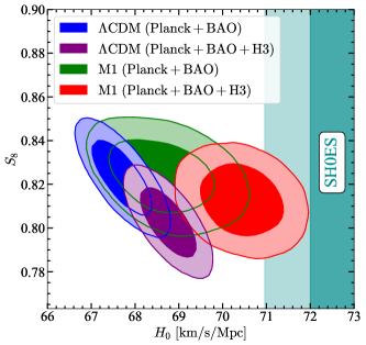
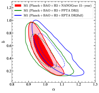
Fig. 2 shows the projected two-dimensional posterior distributions onto the ($H_{0}$, $S_{8}$) plane (left panel) and ($\alpha$, $b$) plane (right panel). In the left panel, we find that M1 model can increase $H_{0}$ value to $70.4\pm 0.6$ and reduce $S_{8}$ value to $0.813\pm 0.01$ for alleviating $H_{0}$ and $S_{8}$ tension. Even without adding H3 likelihood, M1 model (green contour in Fig 2) can also elevate the value of $H_{0}$ in comparison of $\Lambda\rm{CDM}$ model (blue contour in Fig 2). The right panel of Fig. 2 shows a strong correlation between $b$ and $\alpha$. The index $\alpha$ dominates the evolution of the magnetic field, and its impact on the clumping is larger than that of $B_{\rm ch}^{*}$ and $\ell_{\rm ch}^{*}$. Therefore, NANOGrav, PPTA, or EPTA likelihood leads to little discrepancy between the $\alpha-b$ contours. M1 model gives $b=0.51^{+0.17}_{-0.18}$ for three PTA likelihoods, but $\alpha=0.99^{+0.03}_{-0.05}$ for including NANOGrav likelihood, and $\alpha=1.0^{+0.03}_{-0.05}$ for PPTA, and $\alpha=1.0^{+0.04}_{-0.07}$ for EPTA.

Conclusion and Discussion. In this work, we use the NANOGrav 15-year, EPTA DR2full, and PPTA DR3 data to constrain the characteristic strength and scale of the PMFs generated in the early Universe, $B_{\rm ch}^{*}\sim\mathcal{O}(1)~{}\rm{\mu G}$ and $\ell_{\rm ch}^{*}\sim\mathcal{O}(1)~{}\rm{pc}$, assuming that the SGWB can be produced by PMF-induced MHD turbulence. In addition, we employ the model parameter $B^{*}_{\rm ch}$, $\ell^{*}_{\rm ch}$, and the evolution parameter $\alpha$ instead of clumping factor $b$ for Monte Carlo scan. For likelihoods, we have: Planck 2018 (high TT, TE, EE + low EE, TT + lensing), BAO, H3, NANOGrav 15-year, PPTA DR3, and EPTA DR2full. We find that M1 model prefers a clumping factor $b\sim 0.5$, $\alpha\sim 1$, and $B_{\rm ch}^{\rm rec}\sim 0.1{\rm nG}$, which helps to alleviate the $H_{0}$ and $S_{8}$ tension.

Figure 3: The comoving frame strength and the characteristic length of the magnetic fields inferred in our modeling. The red, green, and blue regions correspond to NANOGrav, PPTA, and EPTA results during the QCD phase transition period. The purple region denotes the recombination epoch. The brown dashed line connects the two cosmic times via $B_{\rm ch}\sim\ell_{\rm ch}^{-\alpha}$. The inset plot shows the probability density distribution of characteristic magnetic field strength at recombination era, $B_{\rm ch}^{\rm rec}$. The present value of $B\sim 4\times 10^{-17}$ G, assuming a coherence length of $\sim 1$ Mpc, is inferred from the gamma-ray observations of GRB 221009A Xia:2022uua .

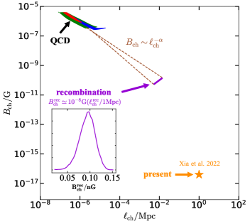
We would like to comment on that the recent observations of the high-energy afterglow of GRB 221009A Xia:2022uua by Fermi-LAT may indicate that there was a delayed cascade emission from very-high-energy photons in the background radiation field, which gives a measurement of the intergalactic magnetic fields at a characteristic scale around $\mathcal{O}(1)$ Mpc with field strength $B_{0}\sim\mathcal{O}(10^{-16})$ G. In Fig 3, we present a summary plot of the magnetic fields at three periods: the QCD phase transition, recombination, and the present epoch. This present value is about five orders of magnitude lower than that needed to alleviate the Hubble tension at the recombination time, suggesting the presence of a very efficient magnetic energy dissipation process. We will leave this topic for future studies.

Acknowledgements We thank Ligong Bian, Karsten Jedamzik, Alberto Roper Pol, Ziqing Xia, and Hong-zhe Zhou for the useful discussion. This work is supported by the National Key Research and Development Program of China (No. 2022YFF0503304), the National Natural Science Foundation of China (No. 12220101003), and the Project for Young Scientists in Basic Research of the Chinese Academy of Sciences (No. YSBR-061).

References

- (1) P. D. Lasky et al., Gravitational-wave cosmology across 29 decades in frequency, Phys. Rev. X 6 (2016) 011035, [1511.05994].
- (2) NANOGrav collaboration, Z. Arzoumanian et al., The NANOGrav 12.5 yr Data Set: Search for an Isotropic Stochastic Gravitational-wave Background, Astrophys. J. Lett. 905 (2020) L34, [2009.04496].
- (3) B. Goncharov et al., On the Evidence for a Common-spectrum Process in the Search for the Nanohertz Gravitational-wave Background with the Parkes Pulsar Timing Array, Astrophys. J. Lett. 917 (2021) L19, [2107.12112].
- (4) S. Chen et al., Common-red-signal analysis with 24-yr high-precision timing of the European Pulsar Timing Array: inferences in the stochastic gravitational-wave background search, Mon. Not. Roy. Astron. Soc. 508 (2021) 4970–4993, [2110.13184].
- (5) J. Antoniadis et al., The International Pulsar Timing Array second data release: Search for an isotropic gravitational wave background, Mon. Not. Roy. Astron. Soc. 510 (2022) 4873–4887, [2201.03980].
- (6) R. W. Hellings and G. S. Downs, Upper Limits on the Isotropic Gravitational Radiation Background from Pulsar Timing Analysis, Astrophys. J. Lett. 265 (1983) L39–L42.
- (7) NANOGrav collaboration, G. Agazie et al., The NANOGrav 15-year Data Set: Evidence for a Gravitational-Wave Background, 2306.16213.
- (8) J. Antoniadis et al., The second data release from the European Pulsar Timing Array III. Search for gravitational wave signals, 2306.16214.
- (9) D. J. Reardon et al., Search for an isotropic gravitational-wave background with the Parkes Pulsar Timing Array, 2306.16215.
- (10) H. Xu et al., Searching for the nano-Hertz stochastic gravitational wave background with the Chinese Pulsar Timing Array Data Release I, 2306.16216.
- (11) M. Rajagopal and R. W. Romani, Ultralow frequency gravitational radiation from massive black hole binaries, Astrophys. J. 446 (1995) 543–549, [astro-ph/9412038].
- (12) A. H. Jaffe and D. C. Backer, Gravitational waves probe the coalescence rate of massive black hole binaries, Astrophys. J. 583 (2003) 616–631, [astro-ph/0210148].
- (13) J. S. B. Wyithe and A. Loeb, Low - frequency gravitational waves from massive black hole binaries: Predictions for LISA and pulsar timing arrays, Astrophys. J. 590 (2003) 691–706, [astro-ph/0211556].
- (14) A. Sesana, F. Haardt, P. Madau and M. Volonteri, Low - frequency gravitational radiation from coalescing massive black hole binaries in hierarchical cosmologies, Astrophys. J. 611 (2004) 623–632, [astro-ph/0401543].
- (15) L. P. Grishchuk, Relic gravitational waves and cosmology, Phys. Usp. 48 (2005) 1235–1247, [gr-qc/0504018].
- (16) S. Vagnozzi, Implications of the NANOGrav results for inflation, Mon. Not. Roy. Astron. Soc. 502 (2021) L11–L15, [2009.13432].
- (17) M. Benetti, L. L. Graef and S. Vagnozzi, Primordial gravitational waves from NANOGrav: A broken power-law approach, Phys. Rev. D 105 (2022) 043520, [2111.04758].
- (18) S. Vagnozzi, Inflationary interpretation of the stochastic gravitational wave background signal detected by pulsar timing array experiments, 2306.16912.
- (19) A. Ashoorioon, K. Rezazadeh and A. Rostami, NANOGrav signal from the end of inflation and the LIGO mass and heavier primordial black holes, Phys. Lett. B 835 (2022) 137542, [2202.01131].
- (20) A. Mazumdar and G. White, Review of cosmic phase transitions: their significance and experimental signatures, Rept. Prog. Phys. 82 (2019) 076901, [1811.01948].
- (21) A. Addazi, Y.-F. Cai, Q. Gan, A. Marciano and K. Zeng, NANOGrav results and dark first order phase transitions, Sci. China Phys. Mech. Astron. 64 (2021) 290411, [2009.10327].
- (22) NANOGrav collaboration, Z. Arzoumanian et al., Searching for Gravitational Waves from Cosmological Phase Transitions with the NANOGrav 12.5-Year Dataset, Phys. Rev. Lett. 127 (2021) 251302, [2104.13930].
- (23) X. Xue et al., Constraining Cosmological Phase Transitions with the Parkes Pulsar Timing Array, Phys. Rev. Lett. 127 (2021) 251303, [2110.03096].
- (24) A. Kobakhidze, C. Lagger, A. Manning and J. Yue, Gravitational waves from a supercooled electroweak phase transition and their detection with pulsar timing arrays, Eur. Phys. J. C 77 (2017) 570, [1703.06552].
- (25) P. Athron, C. Balázs, A. Fowlie, L. Morris and L. Wu, Cosmological phase transitions: from perturbative particle physics to gravitational waves, 2305.02357.
- (26) S. Blasi, V. Brdar and K. Schmitz, Has NANOGrav found first evidence for cosmic strings?, Phys. Rev. Lett. 126 (2021) 041305, [2009.06607].
- (27) J. Ellis and M. Lewicki, Cosmic String Interpretation of NANOGrav Pulsar Timing Data, Phys. Rev. Lett. 126 (2021) 041304, [2009.06555].
- (28) G. Lazarides, R. Maji and Q. Shafi, Cosmic strings, inflation, and gravity waves, Phys. Rev. D 104 (2021) 095004, [2104.02016].
- (29) W. Buchmuller, V. Domcke and K. Schmitz, From NANOGrav to LIGO with metastable cosmic strings, Phys. Lett. B 811 (2020) 135914, [2009.10649].
- (30) C.-F. Chang and Y. Cui, Gravitational waves from global cosmic strings and cosmic archaeology, JHEP 03 (2022) 114, [2106.09746].
- (31) L. Bian, J. Shu, B. Wang, Q. Yuan and J. Zong, Searching for cosmic string induced stochastic gravitational wave background with the Parkes Pulsar Timing Array, Phys. Rev. D 106 (2022) L101301, [2205.07293].
- (32) EPTA collaboration, H. Q. Leclere et al., Practical approaches to analyzing PTA data: Cosmic strings with six pulsars, 2306.12234.
- (33) R. Samanta and S. Datta, Gravitational wave complementarity and impact of NANOGrav data on gravitational leptogenesis, JHEP 05 (2021) 211, [2009.13452].
- (34) S. Datta, A. Ghosal and R. Samanta, Baryogenesis from ultralight primordial black holes and strong gravitational waves from cosmic strings, JCAP 08 (2021) 021, [2012.14981].
- (35) J. Liu, R.-G. Cai and Z.-K. Guo, Large Anisotropies of the Stochastic Gravitational Wave Background from Cosmic Domain Walls, Phys. Rev. Lett. 126 (2021) 141303, [2010.03225].
- (36) L. Bian, S. Ge, C. Li, J. Shu and J. Zong, Searching for Domain Wall Network by Parkes Pulsar Timing Array, 2212.07871.
- (37) V. Vaskonen and H. Veermäe, Did NANOGrav see a signal from primordial black hole formation?, Phys. Rev. Lett. 126 (2021) 051303, [2009.07832].
- (38) V. De Luca, G. Franciolini and A. Riotto, NANOGrav Data Hints at Primordial Black Holes as Dark Matter, Phys. Rev. Lett. 126 (2021) 041303, [2009.08268].
- (39) K. Kohri and T. Terada, Solar-Mass Primordial Black Holes Explain NANOGrav Hint of Gravitational Waves, Phys. Lett. B 813 (2021) 136040, [2009.11853].
- (40) G. Domènech and S. Pi, NANOGrav hints on planet-mass primordial black holes, Sci. China Phys. Mech. Astron. 65 (2022) 230411, [2010.03976].
- (41) T. Papanikolaou and K. N. Gourgouliatos, Constraining supermassive primordial black holes with magnetically induced gravitational waves, 2306.05473.
- (42) Z.-C. Chen, C. Yuan and Q.-G. Huang, Pulsar Timing Array Constraints on Primordial Black Holes with NANOGrav 11-Year Dataset, Phys. Rev. Lett. 124 (2020) 251101, [1910.12239].
- (43) C. Caprini and R. Durrer, Gravitational wave production: A Strong constraint on primordial magnetic fields, Phys. Rev. D 65 (2001) 023517, [astro-ph/0106244].
- (44) C. Caprini and R. Durrer, Gravitational waves from stochastic relativistic sources: Primordial turbulence and magnetic fields, Phys. Rev. D 74 (2006) 063521, [astro-ph/0603476].
- (45) A. Roper Pol, C. Caprini, A. Neronov and D. Semikoz, Gravitational wave signal from primordial magnetic fields in the Pulsar Timing Array frequency band, Phys. Rev. D 105 (2022) 123502, [2201.05630].
- (46) P. Auclair, C. Caprini, D. Cutting, M. Hindmarsh, K. Rummukainen, D. A. Steer et al., Generation of gravitational waves from freely decaying turbulence, JCAP 09 (2022) 029, [2205.02588].
- (47) Planck collaboration, N. Aghanim et al., Planck 2018 results. VI. Cosmological parameters, Astron. Astrophys. 641 (2020) A6, [1807.06209].
- (48) K. Jedamzik and L. Pogosian, Relieving the Hubble tension with primordial magnetic fields, Phys. Rev. Lett. 125 (2020) 181302, [2004.09487].
- (49) K. Jedamzik and A. Saveliev, Stringent Limit on Primordial Magnetic Fields from the Cosmic Microwave Background Radiation, Phys. Rev. Lett. 123 (2019) 021301, [1804.06115].
- (50) A. G. Riess et al., A Comprehensive Measurement of the Local Value of the Hubble Constant with 1 km s-1 Mpc-1 Uncertainty from the Hubble Space Telescope and the SH0ES Team, Astrophys. J. Lett. 934 (2022) L7, [2112.04510].
- (51) M. J. Reid, D. W. Pesce and A. G. Riess, An Improved Distance to NGC 4258 and its Implications for the Hubble Constant, Astrophys. J. Lett. 886 (2019) L27, [1908.05625].
- (52) K. C. Wong et al., H0LiCOW – XIII. A 2.4 per cent measurement of H0 from lensed quasars: 5.3 tension between early- and late-Universe probes, Mon. Not. Roy. Astron. Soc. 498 (2020) 1420–1439, [1907.04869].
- (53) BOSS collaboration, S. Alam et al., The clustering of galaxies in the completed SDSS-III Baryon Oscillation Spectroscopic Survey: cosmological analysis of the DR12 galaxy sample, Mon. Not. Roy. Astron. Soc. 470 (2017) 2617–2652, [1607.03155].
- (54) F. Beutler, C. Blake, M. Colless, D. H. Jones, L. Staveley-Smith, L. Campbell et al., The 6dF Galaxy Survey: Baryon Acoustic Oscillations and the Local Hubble Constant, Mon. Not. Roy. Astron. Soc. 416 (2011) 3017–3032, [1106.3366].
- (55) A. J. Ross, L. Samushia, C. Howlett, W. J. Percival, A. Burden and M. Manera, The clustering of the SDSS DR7 main Galaxy sample – I. A 4 per cent distance measure at , Mon. Not. Roy. Astron. Soc. 449 (2015) 835–847, [1409.3242].
- (56) D. Grasso and H. R. Rubinstein, Revisiting nucleosynthesis constraints on primordial magnetic fields, Phys. Lett. B 379 (1996) 73–79, [astro-ph/9602055].
- (57) T. Kahniashvili, A. G. Tevzadze and B. Ratra, Phase Transition Generated Cosmological Magnetic Field at Large Scales, Astrophys. J. 726 (2011) 78, [0907.0197].
- (58) E. W. Kolb and M. S. Turner, The Early Universe, vol. 69. 1990, 10.1201/9780429492860.
- (59) NANOGRAV collaboration, Z. Arzoumanian et al., The NANOGrav 11-year Data Set: Pulsar-timing Constraints On The Stochastic Gravitational-wave Background, Astrophys. J. 859 (2018) 47, [1801.02617].
- (60) R. Banerjee and K. Jedamzik, The Evolution of cosmic magnetic fields: From the very early universe, to recombination, to the present, Phys. Rev. D 70 (2004) 123003, [astro-ph/0410032].
- (61) K. Subramanian, The origin, evolution and signatures of primordial magnetic fields, Rept. Prog. Phys. 79 (2016) 076901, [1504.02311].
- (62) K. Jedamzik and G. Sigl, The Evolution of the Large-Scale Tail of Primordial Magnetic Fields, Phys. Rev. D 83 (2011) 103005, [1012.4794].
- (63) R. Durrer and A. Neronov, Cosmological Magnetic Fields: Their Generation, Evolution and Observation, Astron. Astrophys. Rev. 21 (2013) 62, [1303.7121].
- (64) D. N. Hosking and A. A. Schekochihin, Reconnection-Controlled Decay of Magnetohydrodynamic Turbulence and the Role of Invariants, Phys. Rev. X 11 (2021) 041005, [2012.01393].
- (65) A. Brandenburg, H. Zhou and R. Sharma, Batchelor, Saffman, and Kazantsev spectra in galactic small-scale dynamos, Mon. Not. Roy. Astron. Soc. 518 (2022) 3312–3325, [2207.09414].
- (66) M. Rashkovetskyi, J. B. Muñoz, D. J. Eisenstein and C. Dvorkin, Small-scale clumping at recombination and the Hubble tension, Phys. Rev. D 104 (2021) 103517, [2108.02747].
- (67) D. Blas, J. Lesgourgues and T. Tram, The Cosmic Linear Anisotropy Solving System (CLASS) II: Approximation schemes, JCAP 07 (2011) 034, [1104.2933].
- (68) T. Brinckmann and J. Lesgourgues, MontePython 3: boosted MCMC sampler and other features, Phys. Dark Univ. 24 (2019) 100260, [1804.07261].
- (69) B. Audren, J. Lesgourgues, K. Benabed and S. Prunet, Conservative Constraints on Early Cosmology: an illustration of the Monte Python cosmological parameter inference code, JCAP 02 (2013) 001, [1210.7183].
- (70) Z.-Q. Xia, Y. Wang, Q. Yuan and Y.-Z. Fan, An inter-galactic magnetic field strength of G inferred with GRB 221009A, 2210.13052.