Are Neurons Actually Collapsed? On the Fine-Grained Structure in
Neural Representations

Yongyi Yang    Jacob Steinhardt    Wei Hu
Abstract

Recent work has observed an intriguing “Neural Collapse” phenomenon in well-trained neural networks, where the last-layer representations of training samples with the same label collapse into each other. This appears to suggest that the last-layer representations are completely determined by the labels, and do not depend on the intrinsic structure of input distribution. We provide evidence that this is not a complete description, and that the apparent collapse hides important fine-grained structure in the representations. Specifically, even when representations apparently collapse, the small amount of remaining variation can still faithfully and accurately captures the intrinsic structure of input distribution. As an example, if we train on CIFAR-10 using only 5 coarse-grained labels (by combining two classes into one super-class) until convergence, we can reconstruct the original 10-class labels from the learned representations via unsupervised clustering. The reconstructed labels achieve 93%percent9393\% accuracy on the CIFAR-10 test set, nearly matching the normal CIFAR-10 accuracy for the same architecture. We also provide an initial theoretical result showing the fine-grained representation structure in a simplified synthetic setting. Our results show concretely how the structure of input data can play a significant role in determining the fine-grained structure of neural representations, going beyond what Neural Collapse predicts.

Machine Learning, ICML

1 Introduction

Much of the success of deep neural networks has, arguably, been attributed to their ability to learn useful representations, or features, of the data (Rumelhart et al., 1985). Although neural networks are often trained to optimize a single objective function with no explicit requirements on the inner representations, there is ample evidence suggesting that these learned representations contain rich information about the input data (Levy & Goldberg, 2014; Olah et al., 2017). As a result, formally characterizing and understanding the structural properties of neural representations is of great theoretical and practical interest, and can provide insights on how deep learning works and how to make better use of these representations.

One intriguing phenomenon recently discovered by Papyan et al. (2020) is Neural Collapse, which identifies structural properties of last-layer representations during the terminal phase of training (i.e. after zero training error is reached). The simplest of these properties is that the last-layer representations for training samples with the same label collapse into a single point, which is referred to as “variability collapse (NC1).” This is surprising, since the collapsed structure is not necessary to achieve small training or test error, yet it arises consistently in standard architectures trained on standard classification datasets.

A series of recent papers were able to theoretically explain Neural Collapse under a simplified model called the unconstrained feature model or layer-peeled model (see Section 2 for a list of references). In this model, the last-layer representation of each training sample is treated as a free optimization variable and therefore the training loss essentially has the form of a matrix factorization. Under a variety of different setups, it was proved that the solution to this simplified problem should satisfy Neural Collapse. Although Neural Collapse is relatively well understood in this simplified model, this model completely ignores the role of the input data because the loss function is independent of the input data. Conceptually, this suggests that Neural Collapse is only determined by the labels and may happen regardless of the input data distribution. Zhu et al. (2021) provided further empirical support of this claim via a random labeling experiment.

On the other hand, it is conceivable that the intrinsic structure of the input distribution should play a role in determining the structure of neural net representations. For example, if a class contains a heterogeneous set of input data (such as different subclasses), it is possible that their heterogeneity is also respected in their feature representations (Sohoni et al., 2020). However, this appears to contradict Neural Collapse, because Neural Collapse would predict that all the representations collapse into each other as long as they have the same class label. This dilemma motivates us to study the following main question in this paper:

How can we reconcile the roles of the intrinsic structure of input distribution vs. the explicit structure of the labels in determining the last-layer representations in neural networks?
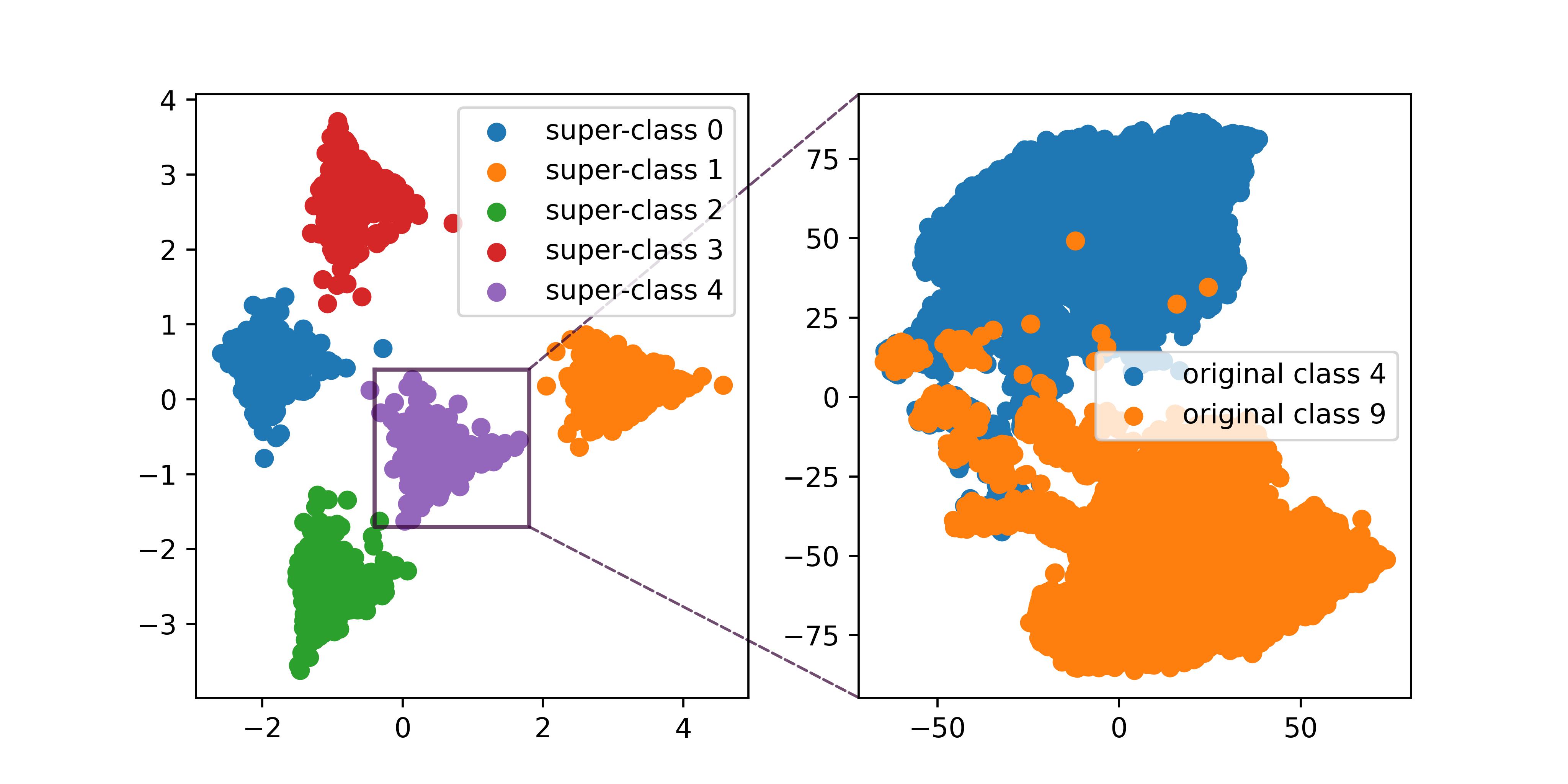
Refer to caption
Figure 1: Fine-grained clustering structure of the last-layer representations of ResNet-18 trained on Coarse CIFAR-10 (5 super-classes). Left figure: PCA visualization for all training samples. Right figure: t-SNE visualization for all training samples in super-class 4 (which consists of original classes 4 and 9).

Our methodology and findings.

To study the above question, we design experiments to manually create a mismatch between the intrinsic structure of the input distribution and the explicit labels provided for training in standard classification datasets and measure how the last-layer representations behave in response to our interventions. This allows us to isolate the effect of the input distribution from the effect of labels. As an illustrative example, for the CIFAR-10 dataset (a 10-class classification task), we alter its labels in two different ways, resulting in a coarsely-labeled and a finely-labeled version:

  • Coarse CIFAR-10: combine every two class labels into one and obtain a 5-class task (see Figure 2 for an illustration);

  • Fine CIFAR-10: split every class label randomly into two labels and obtain a 20-class task.

We train standard network architectures (e.g. ResNet, DenseNet) using SGD on these altered datasets. Our main findings are summarized below.

First, both the intrinsic structure of the input distribution and the explicit labels provided in training clearly affect the structure of the last-layer representations. The effect of input distribution emerges earlier in training, while the effect of labels appears at a later stage. For example, for both Coarse CIFAR-10 and Fine CIFAR-10, at some point the representations naturally form 10 clusters according to the original CIFAR-10 labels (which comes from the intrinsic input structure), even though 5 or 20 different labels are provided for training. Later in training (after 100% training accuracy is reached), the representations collapse into 5 or 20 clusters driven by the explicit labels provided, as predicted by Neural Collapse.

Second, even after Neural Collapse has occurred according to the explicit label information, the seemingly collapsed representations corresponding to each label can still exhibit fine-grained structures determined by the input distribution. As an illustration, Figure 1 visualizes the representations from the last epoch of training a ResNet-18 on Coarse CIFAR-10. While globally there are 5 separated clusters as predicted by Neural Collapse, if we zoom in on each cluster, it clearly consists of two subclusters which correspond to the original CIFAR-10 classes. We also find that this phenomenon persists even after a very long training period (e.g. 1,000 epochs), indicating that the effect of input distribution is not destroyed by that of the labels, at least not within a normal training budget.

To further validate our finding that significant input information is present in the last-layer representations despite Neural Collapse, we perform a simple Cluster-and-Linear-Probe (CLP) procedure on the representations from ResNet-18 trained on Coarse CIFAR-10, in which we use an unsupervised clustering method to reconstruct the original labels, and then train a linear classifier on top of these representations using the reconstructed labels. We find that CLP can achieve >93%absentpercent93>93\% accuracy on the original CIFAR-10 test set, matching the standard accuracy of ResNet-18, even though only 5 coarse labels are provided the entire time.

Theoretical result in a synthetic setting.

To complement our findings, we provide a theoretical explanation of the fine-grained representation structure in a simplified synthetic setting — a one-hidden-layer neural network trained on coarsely labeled Gaussian mixture data. We prove that such a network trained by gradient descent produces separable hidden-layer representations for different clusters even if they are given the same label for training.

Takeaway.

While Neural Collapse is an intriguing phenomenon that consistently happens, we provide concrete evidence showing that it is not the most comprehensive description of the behavior of last-layer representations in practice, as it fails to capture the possible fine-grained properties determined by the intrinsic structure of the input distribution.

2 Related Work

The Neural Collapse phenomenon was originally discovered by Papyan et al. (2020), and has led to a series of further investigations.

A number of papers Fang et al. (2021); Lu & Steinerberger (2020); Wojtowytsch et al. (2020); Mixon et al. (2022); Zhu et al. (2021); Ji et al. (2021); Han et al. (2021); Zhou et al. (2022); Tirer & Bruna (2022); Yaras et al. (2022) studied a simplified unconstrained feature model, also known as layer-peeled model, and showed that Neural Collapse provably happens under a variety of settings. This model treats the last-layer representations of all training samples as free optimization variables. By doing this, the loss function no longer depends on the input data, and therefore this line of work is unable to capture any effect of the input distribution on the structure of the representations. Ergen & Pilanci (2021); Tirer & Bruna (2022); Weinan & Wojtowytsch (2022) considered more complicated models but still did not incorporate the role of the input distribution.

Hui et al. (2022) studied the connection of Neural Collapse to generalization and concluded that Neural Collapse occurs only on the training set, not on the test set. Galanti et al. (2021) found that Neural Collapse does generalize to test samples as well as new classes, and used this observation to study transfer learning and few-shot learning.

Sohoni et al. (2020) observed that the last-layer representations of different subclasses within the same class are often separated into different clusters, and used this observation to design an algorithm for improving group robustness. The fine-grained representation phenomenon we observe is in a qualitatively different regime from that of Sohoni et al. (2020). First of all, we focus on the Neural Collapse regime and find that fine-grained representation structure can co-exist with Neural Collapse. Furthermore, Sohoni et al. (2020) looked at settings in which different subclasses have very different accuracies and explicitly attributed the representation separability phenomenon to this performance difference. On the other hand, we find that representation separability can happen even when there is no performance gap between different subclasses.

3 Preliminaries and Setup

Consider a classification dataset 𝒟={(𝒙k,yk)}k=1n𝒟superscriptsubscriptsubscript𝒙𝑘subscript𝑦𝑘𝑘1𝑛\mathcal{D}=\{(\mbox{\boldmath$x$}_{k},y_{k})\}_{k=1}^{n}, where (𝒙k,yk)d×[C]subscript𝒙𝑘subscript𝑦𝑘superscriptsuperscript𝑑delimited-[]𝐶(\mbox{\boldmath$x$}_{k},y_{k})\in\mathbb{R}^{d^{\prime}}\times[C] is a pair of input features and label, n𝑛n is the number of samples, dsuperscript𝑑d^{\prime} is the input dimension, and C𝐶C is the number of classes. Here [C]={1,,C}delimited-[]𝐶1𝐶[C]=\{1,\ldots,C\}.

For a given neural network, we denote its last-layer representations corresponding to the dataset 𝒟𝒟\mathcal{D} by Hn×d𝐻superscript𝑛𝑑H\in\mathbb{R}^{n\times d}, i.e. the hidden representation before the final linear transformation, where d𝑑d is the last-layer dimensionality. For an original class c[C]𝑐delimited-[]𝐶c\in[C], we denote the number of samples in class c𝑐c by ncsubscript𝑛𝑐n_{c}, and the last-layer representation of k𝑘k-th sample in class c𝑐c by 𝒉k(c)subscriptsuperscript𝒉𝑐𝑘{\boldsymbol{h}}^{(c)}_{k}.

3.1 Preliminaries of Neural Collapse

Neural Collapse (Papyan et al., 2020) characterizes 4 phenomena, named NC1-NC4. Here we introduce NC1 and NC2 which concern the structure of the last-layer representations.

NC1, or variability collapse, asserts that the variance of last-layer representations of samples within the same class vanishes as training proceeds. Formally, it can be measured by 𝖭𝖢𝟣=1CTr(ΣWΣB)subscript𝖭𝖢11𝐶TrsubscriptΣ𝑊superscriptsubscriptΣ𝐵\mathsf{NC_{1}}=\frac{1}{C}\mathrm{Tr}\left({\Sigma}_{W}{\Sigma}_{B}^{\dagger}\right) (Papyan et al., 2020; Zhu et al., 2021), which is observed to go to 00. Here ΣWsubscriptΣ𝑊{{\Sigma}}_{W} and ΣBsubscriptΣ𝐵{{\Sigma}}_{B} are defined as

ΣW=1Cc[C]1nci=1nc(𝒉i(c)𝝁c)(𝒉i(c)𝝁c)subscriptΣ𝑊1𝐶subscript𝑐delimited-[]𝐶1subscript𝑛𝑐superscriptsubscript𝑖1subscript𝑛𝑐superscriptsubscript𝒉𝑖𝑐subscript𝝁𝑐superscriptsuperscriptsubscript𝒉𝑖𝑐subscript𝝁𝑐top{\Sigma}_{W}=\frac{1}{C}\sum_{c\in[C]}\frac{1}{n_{c}}\sum_{i=1}^{n_{c}}\left(\mbox{\boldmath$h$}_{i}^{(c)}-\boldsymbol{\mu}_{c}\right)\left(\mbox{\boldmath$h$}_{i}^{(c)}-\boldsymbol{\mu}_{c}\right)^{\top} (1)

and

ΣB=1Cc[C](𝝁c𝝁G)(𝝁c𝝁G),subscriptΣ𝐵1𝐶subscript𝑐delimited-[]𝐶subscript𝝁𝑐subscript𝝁𝐺superscriptsubscript𝝁𝑐subscript𝝁𝐺top{\Sigma}_{B}=\frac{1}{C}\sum_{c\in[C]}\left({\boldsymbol{\mu}}_{c}-{\boldsymbol{\mu}}_{G}\right)\left({\boldsymbol{\mu}}_{c}-{\boldsymbol{\mu}}_{G}\right)^{\top}, (2)

where 𝝁c=1nck=1nc𝒉k(c)subscript𝝁𝑐1subscript𝑛𝑐superscriptsubscript𝑘1subscript𝑛𝑐superscriptsubscript𝒉𝑘𝑐{\boldsymbol{\mu}}_{c}=\frac{1}{n_{c}}\sum_{k=1}^{n_{c}}{\boldsymbol{h}}_{k}^{(c)} are the class means and 𝝁G=1nc=1Ck=1nc𝒉k(c)subscript𝝁𝐺1𝑛superscriptsubscript𝑐1𝐶superscriptsubscript𝑘1subscript𝑛𝑐superscriptsubscript𝒉𝑘𝑐{\boldsymbol{\mu}}_{G}=\frac{1}{n}\sum_{c=1}^{C}\sum_{k=1}^{n_{c}}{\boldsymbol{h}}_{k}^{(c)} is the global mean.

NC2 predicts that the class means form a special structure, namely, their normalized covariance converges to the Simplex Equiangular Tight Frame (ETF). This can be characterize by

𝖭𝖢𝟤=defMMMM1C1(I1C𝟏C𝟏C)0subscript𝖭𝖢2defsubscriptnorm𝑀superscript𝑀topsubscriptnorm𝑀superscript𝑀top1𝐶1𝐼1𝐶subscript1𝐶superscriptsubscript1𝐶top0\mathsf{NC_{2}}\overset{\text{def}}{=}\left\|\frac{MM^{\top}}{\left\|MM^{\top}\right\|_{\mathcal{F}}}-\frac{1}{\sqrt{C-1}}\left(I-\frac{1}{C}{\boldsymbol{1}}_{C}{\boldsymbol{1}}_{C}^{\top}\right)\right\|_{\mathcal{F}}\to 0 (3)

during training, where MC×d𝑀superscript𝐶𝑑M\in\mathbb{R}^{C\times d} is the stack of centralized class-means, whose c𝑐c-th row is 𝝁c𝝁Gsubscript𝝁𝑐subscript𝝁𝐺{\boldsymbol{\mu}}_{c}-{\boldsymbol{\mu}}_{G}, and 𝟙CCsubscript1𝐶superscript𝐶\mathbbm{1}_{C}\in\mathbbm{R}^{C} is the all-one vector, and I𝐼I is the identity matrix.

3.2 Experiment Setup

In our experiment, we explore the role of input distribution and labels through assigning coarser or finer labels to each sample, and then explore the structure of last-layer representation of a model trained on the dataset with coarse or fine labels and see to what extent the information of original labels are preserved.

The coarse labels are created in the following way. Choose a number C~~𝐶\tilde{C} divides C𝐶C, and create coarse labels by

y~k=ykmodC~,subscript~𝑦𝑘subscript𝑦𝑘mod~𝐶\tilde{y}_{k}=y_{k}\mathop{\mathrm{mod}}\tilde{C}, (4)

which merges the classes whose indices have the same remainder w.r.t. C~~𝐶\tilde{C} and thus creates C~~𝐶\tilde{C} super-classes. Since the original indices of classes generally have no special meanings, this process should act similarly to randomly merging classes.111We adopt this deterministic process for simplicity and reproducibility. However, we do provide additional results with random merging in Appendix F. We say the samples with the same coarse label belong to the same super-class, and call the dataset 𝒟~={(xk,y~k)}k=1n~𝒟superscriptsubscriptsubscript𝑥𝑘subscript~𝑦𝑘𝑘1𝑛\tilde{\mathcal{D}}=\{(x_{k},\tilde{y}_{k})\}_{k=1}^{n} the coarse dataset, which we use to train the model. Figure 2 provides an illustration of the coarse labels on CIFAR-10 with C~=5~𝐶5\tilde{C}=5, which we call Coarse CIFAR-10.

Refer to caption
Figure 2: Illustration of Coarse CIFAR-10.

To create fine labels, we randomly split each class into two sub-classes. Specifically, the fine labels are created by

y^k=yk+βC,subscript^𝑦𝑘subscript𝑦𝑘𝛽𝐶\hat{y}_{k}=y_{k}+\beta C, (5)

where y^ksubscript^𝑦𝑘\hat{y}_{k} is the fine label of sample k𝑘k and C𝐶C is the number of original classes and β𝛽\beta is a Bernoulli Variable. This process result in a dataset 𝒟^={(xk,y^k)}k=1n^𝒟superscriptsubscriptsubscript𝑥𝑘subscript^𝑦𝑘𝑘1𝑛\hat{\mathcal{D}}=\left\{\left(x_{k},\hat{y}_{k}\right)\right\}_{k=1}^{n} with 2C2𝐶2C classes. Same as before, we call 𝒟^^𝒟\hat{\mathcal{D}} the fine dataset.

4 Exploring the Fine-Grained Representation Structure with Coarse CIFAR-10

In this section, we experiment with coarsely labeled datasets, using Coarse CIFAR-10 as an illustrative example. Specifically, the model is trained on the training set of Coarse CIFAR-10 for a certain number of steps that is sufficient for the model to converge. We then take the last-layer representations of the model throughout training and explore their structure.

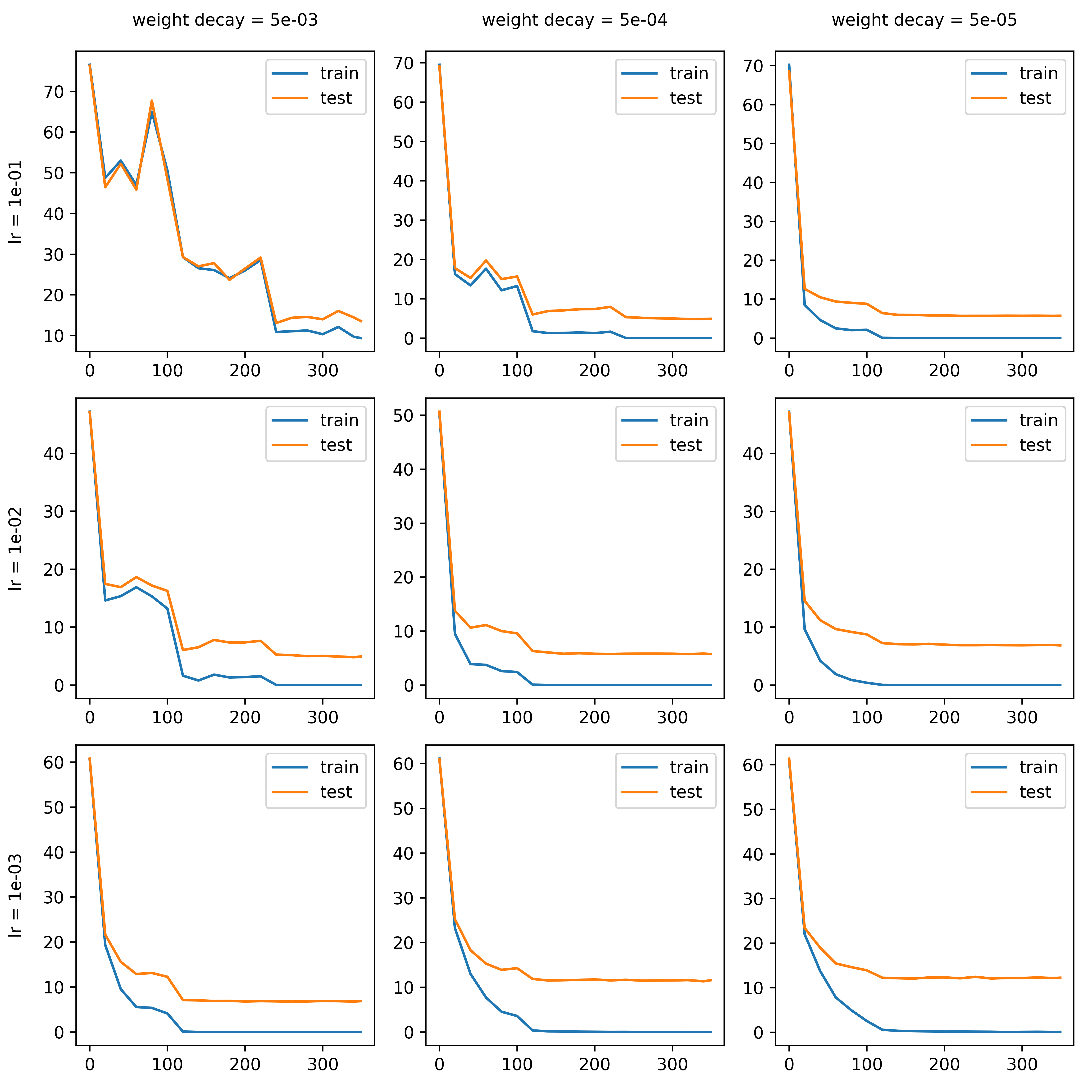
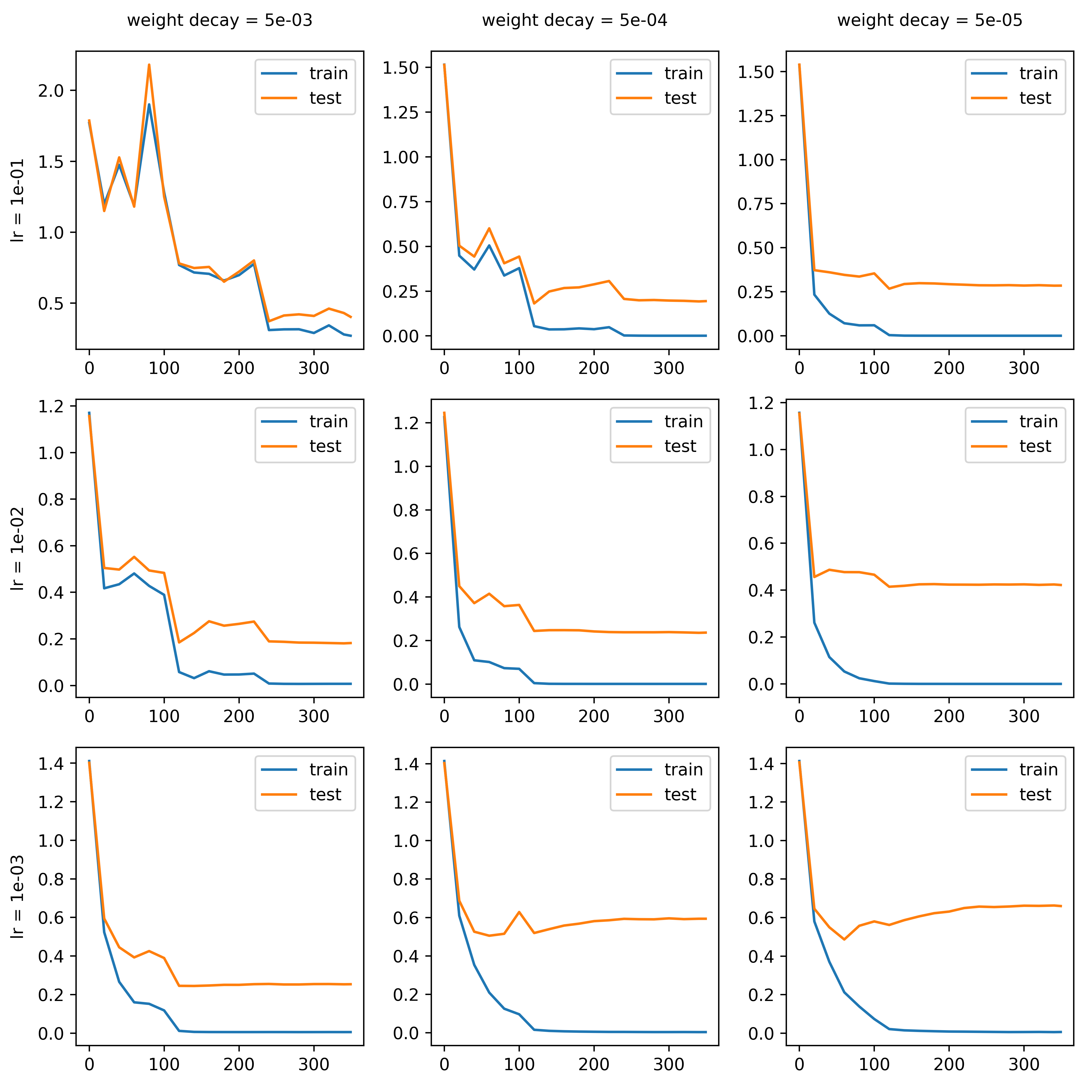
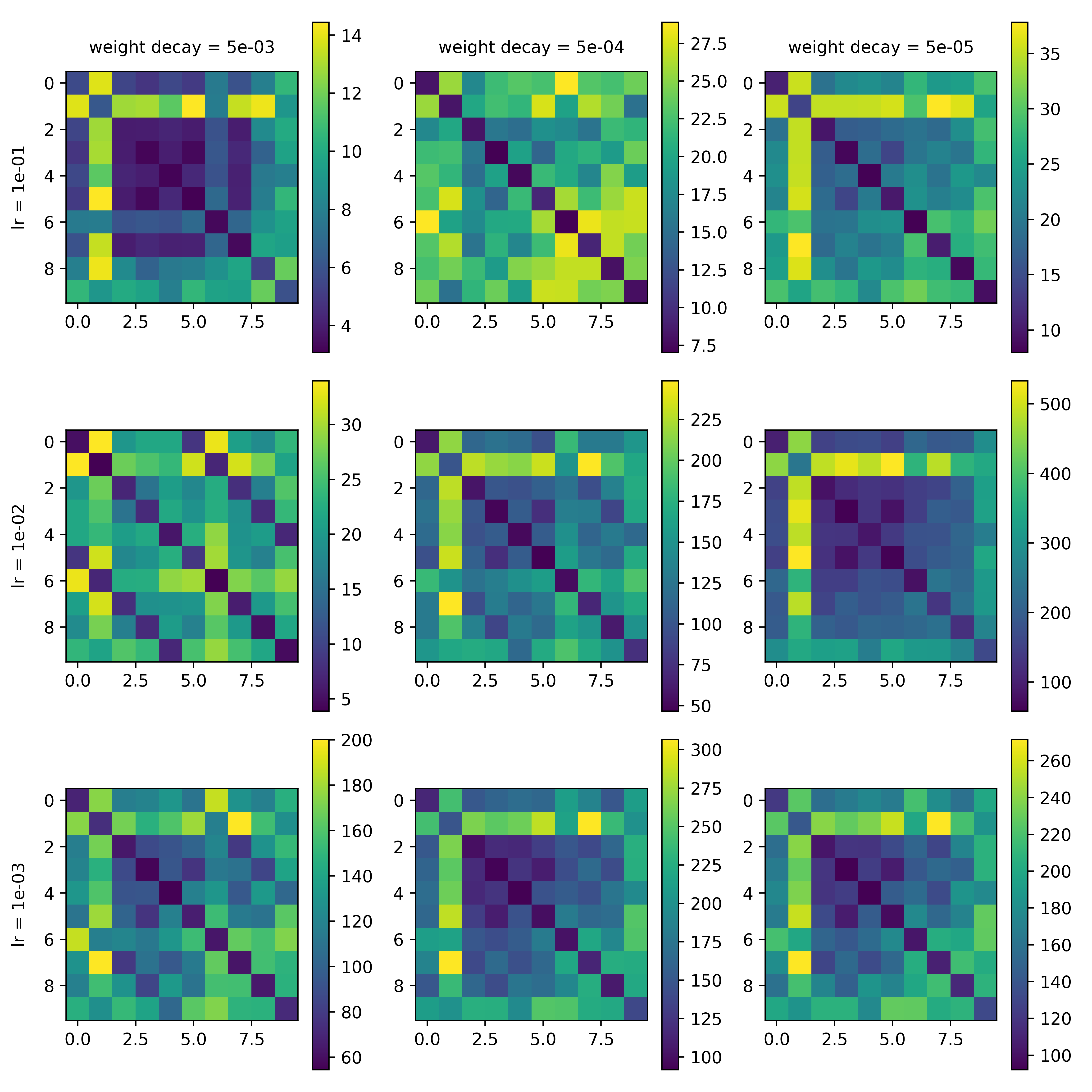
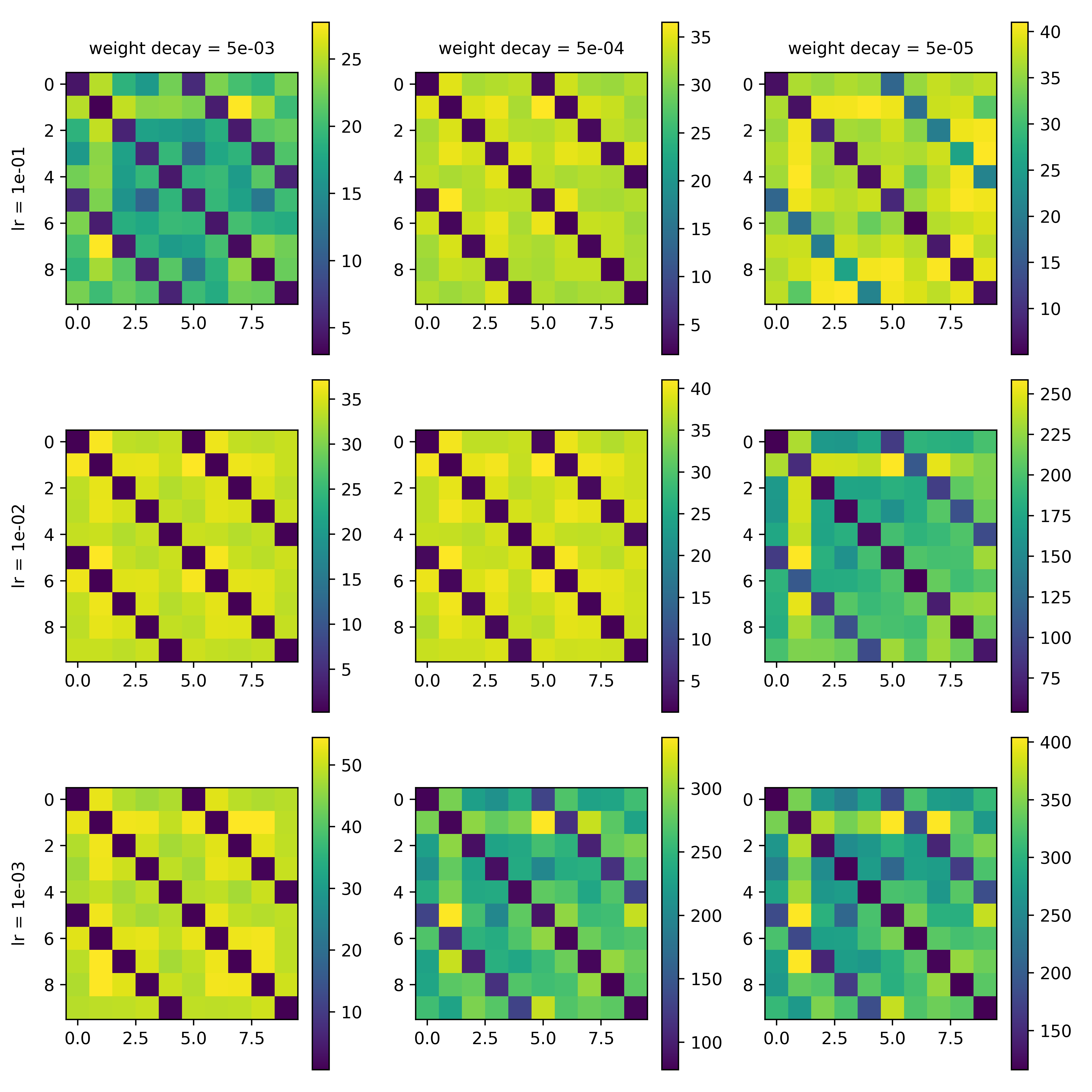
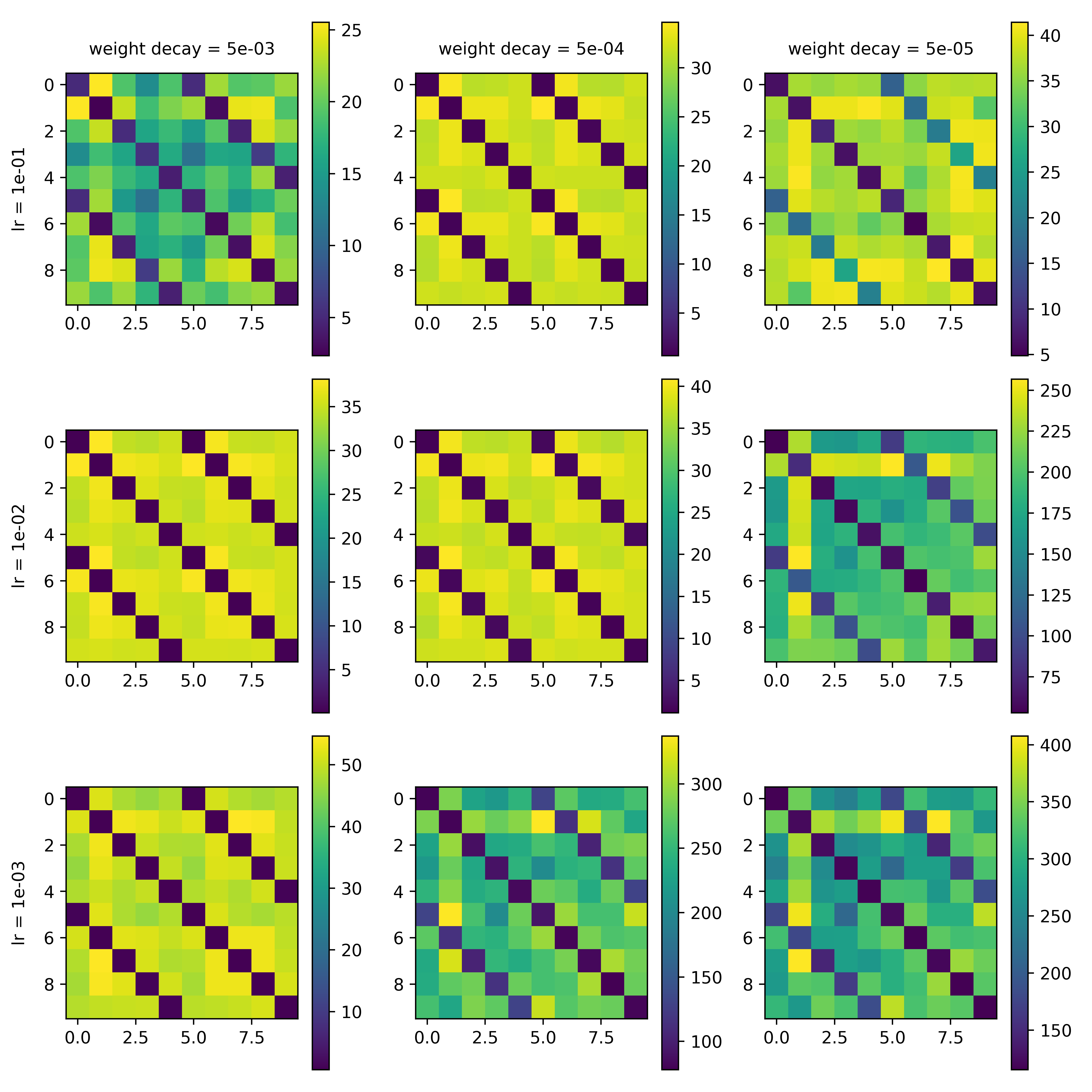
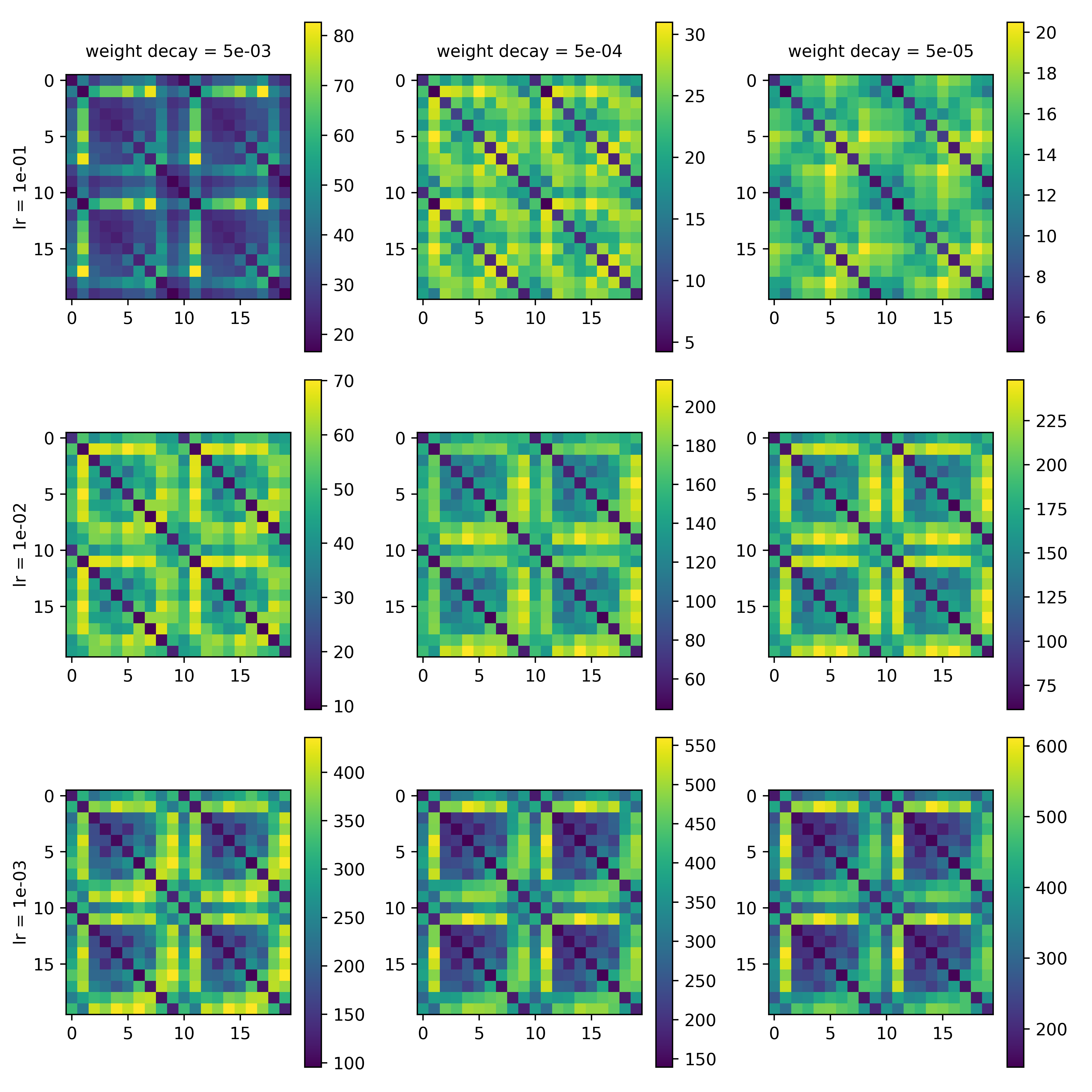
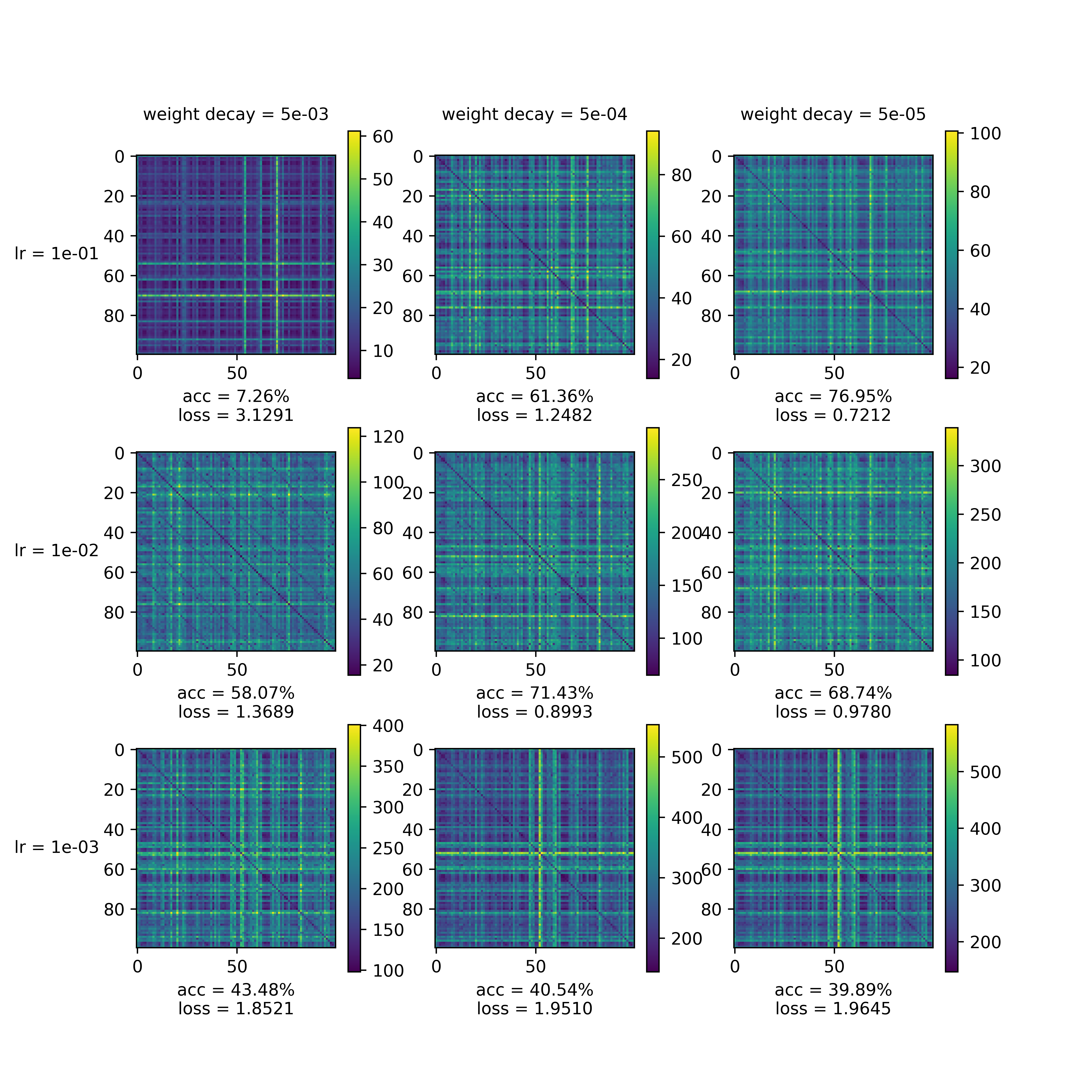
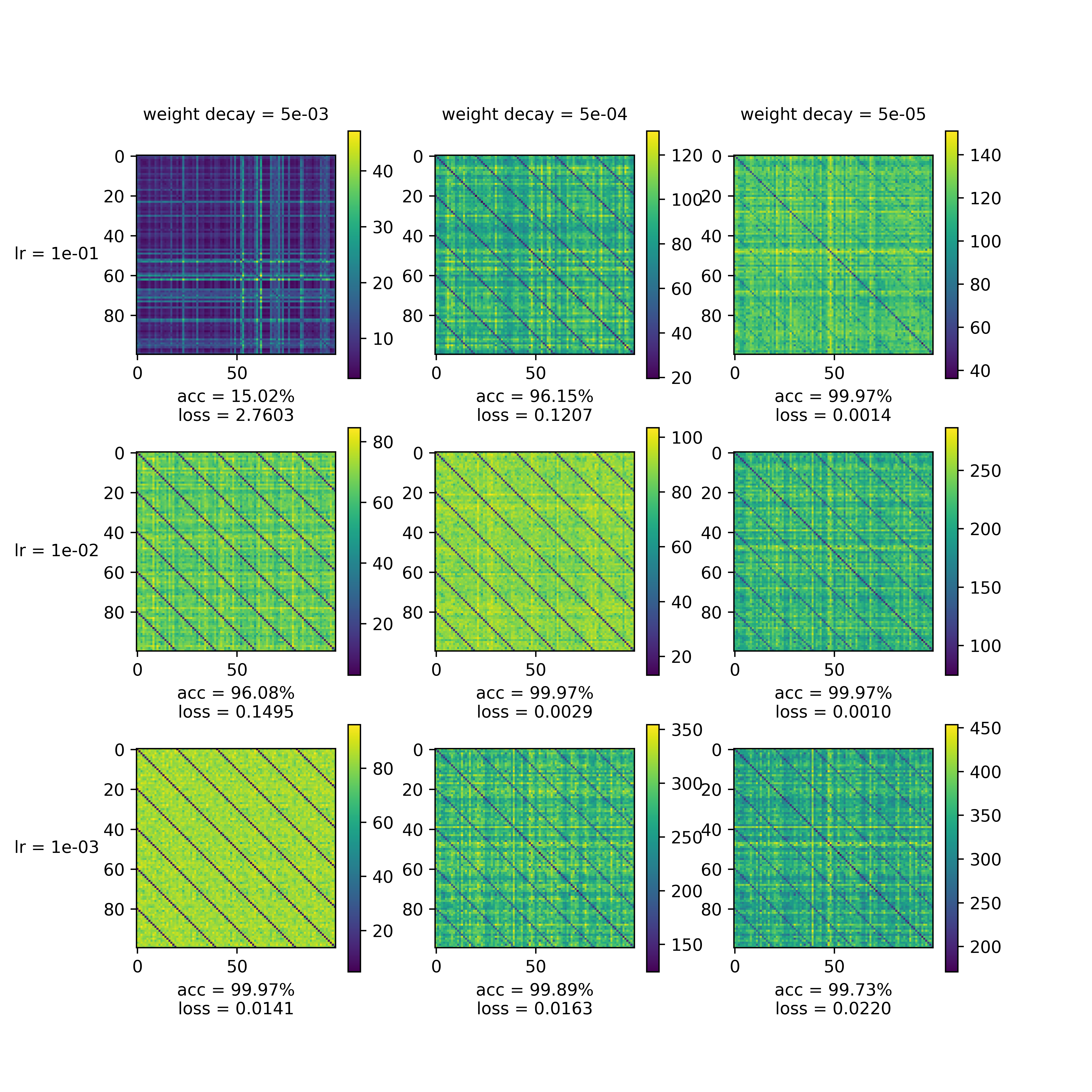
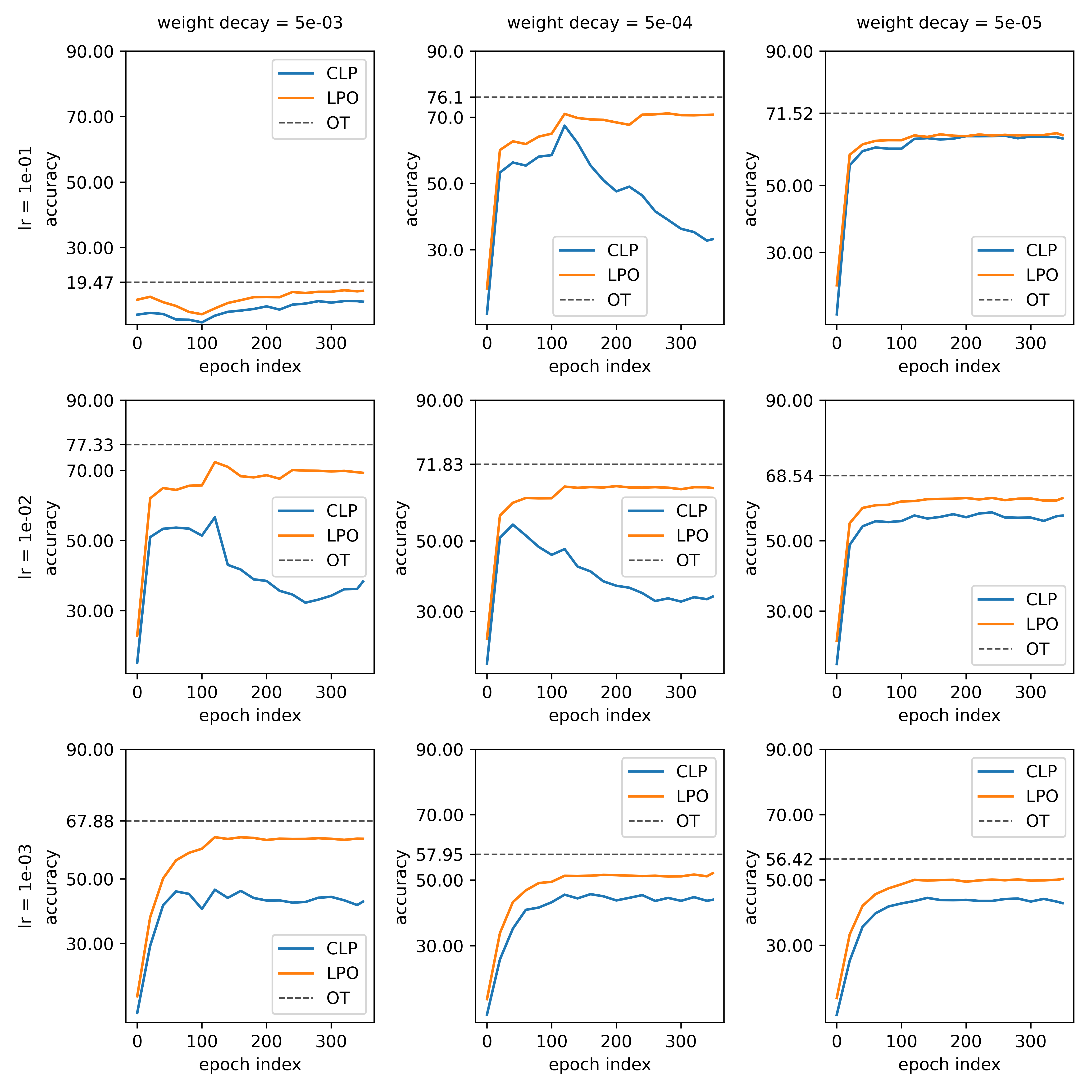
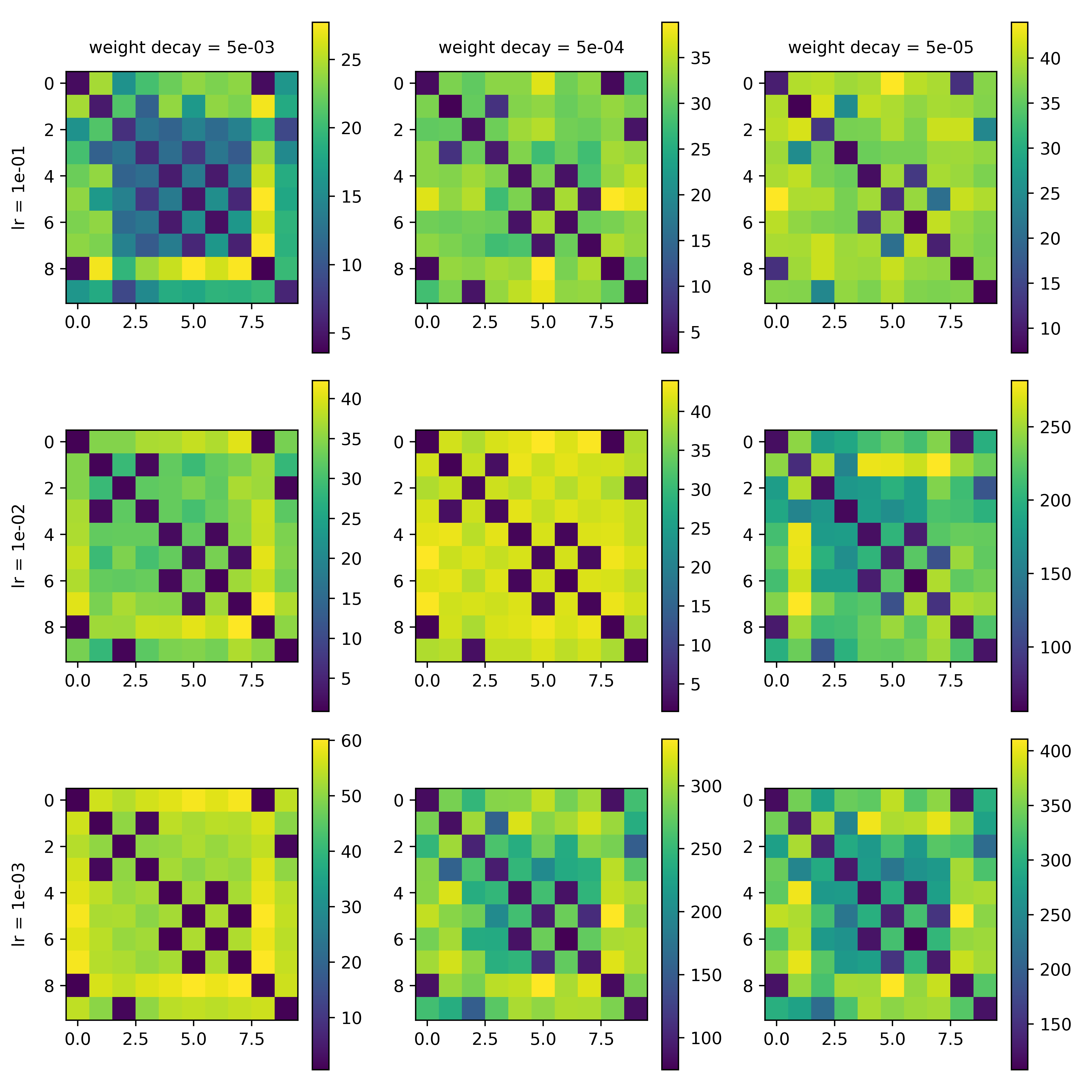
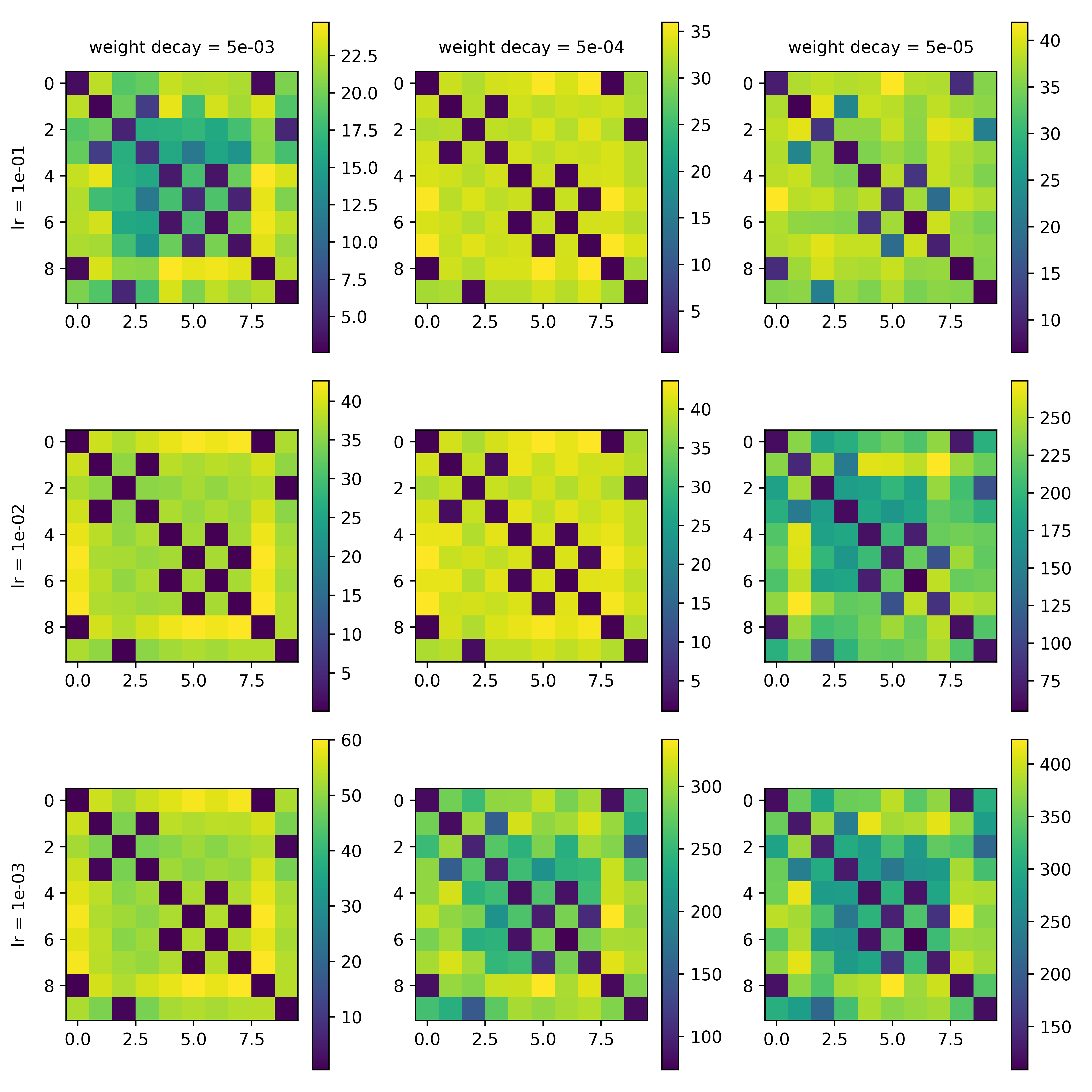
In order to make an exhaustive observation, the experiments are performed using different learning rates and weight-decay rates. Specifically, we choose the initial learning rate in {101,102,103}superscript101superscript102superscript103\{10^{-1},10^{-2},10^{-3}\} (we apply a standard learning rate decay schedule) and the weight-decay rate in {5×103,5×104,5×105}5superscript1035superscript1045superscript105\{5\times 10^{-3},5\times 10^{-4},5\times 10^{-5}\} and run all 9 possible combinations of them. The experiments are also conducted on multiple datasets and network architectures. Due to space limit, we defer complete results to Appendix (see Appendices C, E and F). In this section we focus on ResNet-18 on Coarse CIFAR-10, where the original number of classes is C=10𝐶10C=10 and the number of coarse labels is C~=5~𝐶5\tilde{C}=5. In this section, we only report results for one group of representative hyper-parameter combinations: learning rate is 0.10.10.1 and weight-decay rate is 5×1045superscript1045\times 10^{-4}. Results for other hyper-parameters are presented in Appendices C, D, E, F, G and H.

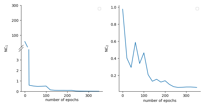
First, we verify that Neural Collapse does happen, i.e. the representations converge to 555 clusters, and the class means form a Simplex ETF structure. Specifically, we measure 𝖭𝖢𝟣subscript𝖭𝖢1\mathsf{NC_{1}} and 𝖭𝖢𝟤subscript𝖭𝖢2\mathsf{NC_{2}} defined in Section 3.1, with C𝐶C replaced by C~~𝐶\tilde{C} since we are calculating it on the coarsely labeled dataset. The results are shown in Figure 3, which matches previous results in Papyan et al. (2020); Zhu et al. (2021), which verify Neural Collapse happens.
Refer to caption
Figure 3: The value of NC1subscriptNC1\mathrm{NC}_{1} and NC2subscriptNC2\mathrm{NC}_{2} w.r.t. number of training epochs.

4.1 Class Distance

Now, we look at the average square Euclidian distance of last-layer representations between each two original classes. Formally, we calculate a class distance matrix DC×C𝐷superscript𝐶𝐶D\in\mathbb{R}^{C\times C}, whose entries are

Di,j=1ninju=1niv=1nj𝒉u(i)𝒉v(j)22,subscript𝐷𝑖𝑗1subscript𝑛𝑖subscript𝑛𝑗superscriptsubscript𝑢1subscript𝑛𝑖superscriptsubscript𝑣1subscript𝑛𝑗superscriptsubscriptnormsubscriptsuperscript𝒉𝑖𝑢subscriptsuperscript𝒉𝑗𝑣22D_{i,j}=\frac{1}{n_{i}n_{j}}\sum_{u=1}^{n_{i}}\sum_{v=1}^{n_{j}}\left\|\mbox{\boldmath$h$}^{(i)}_{u}-\mbox{\boldmath$h$}^{(j)}_{v}\right\|_{2}^{2}, (6)

for all i,j[C]𝑖𝑗delimited-[]𝐶i,j\in[C], where 𝒉k(c)superscriptsubscript𝒉𝑘𝑐{\boldsymbol{h}}_{k}^{(c)} represents the last-layer representation of the k𝑘k-th sample of super-class u𝑢u.

Refer to caption
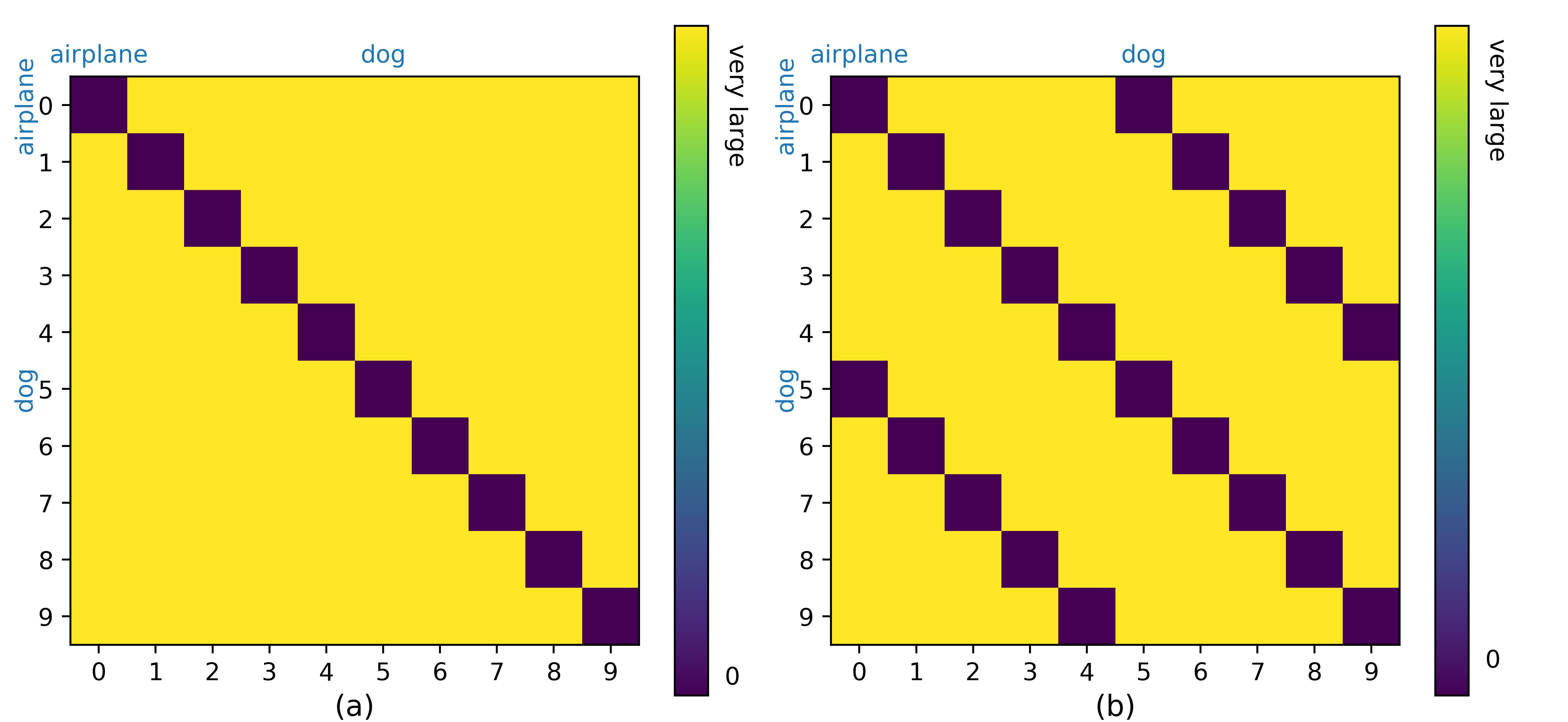
Figure 4: An illustration of predicted class distance matrix heatmaps of Coarse CIFAR-10, each row and column represents an original class. (a): If input distribution dominates the last-layer representations. (b): If Neural Collapse dominates the last-layer representations.

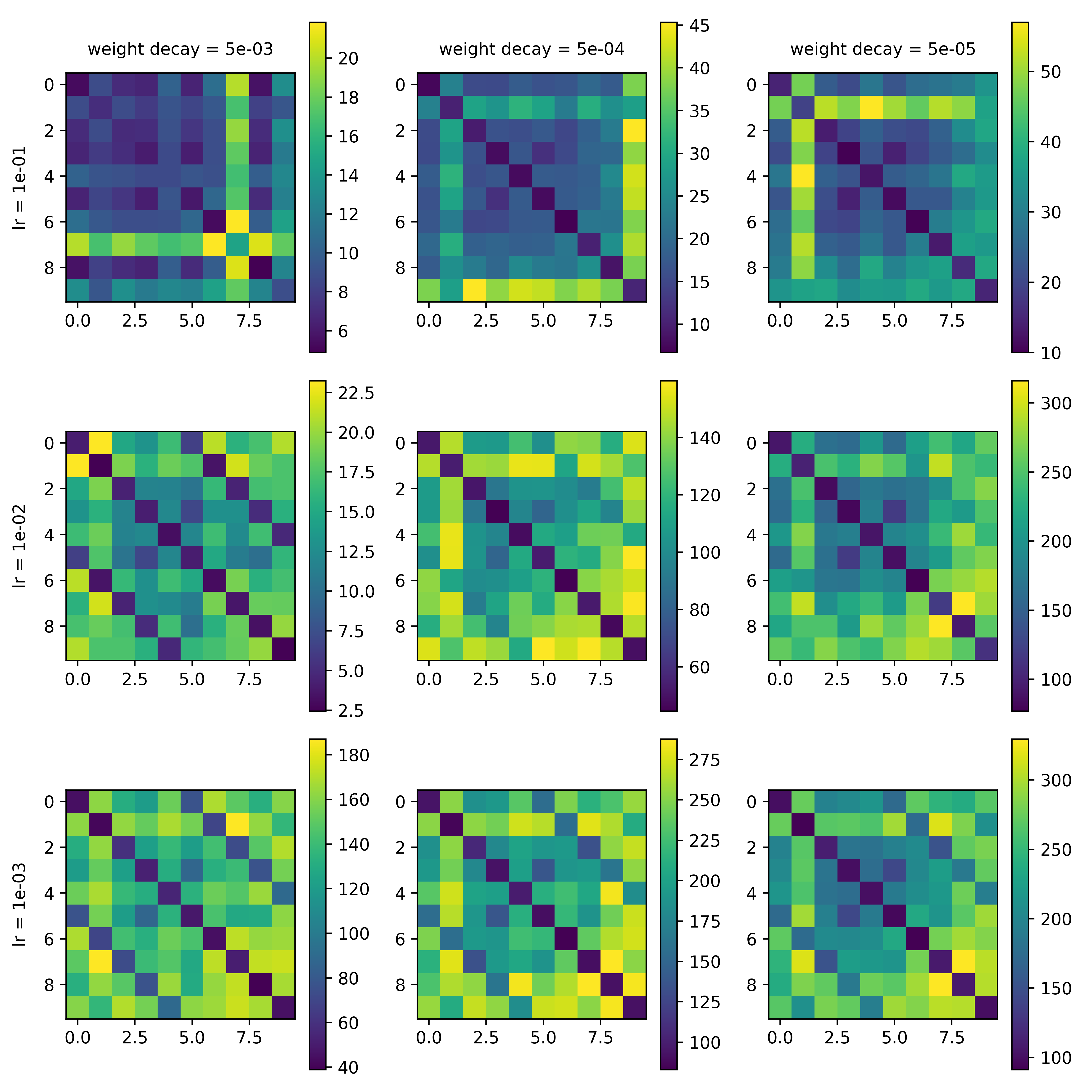
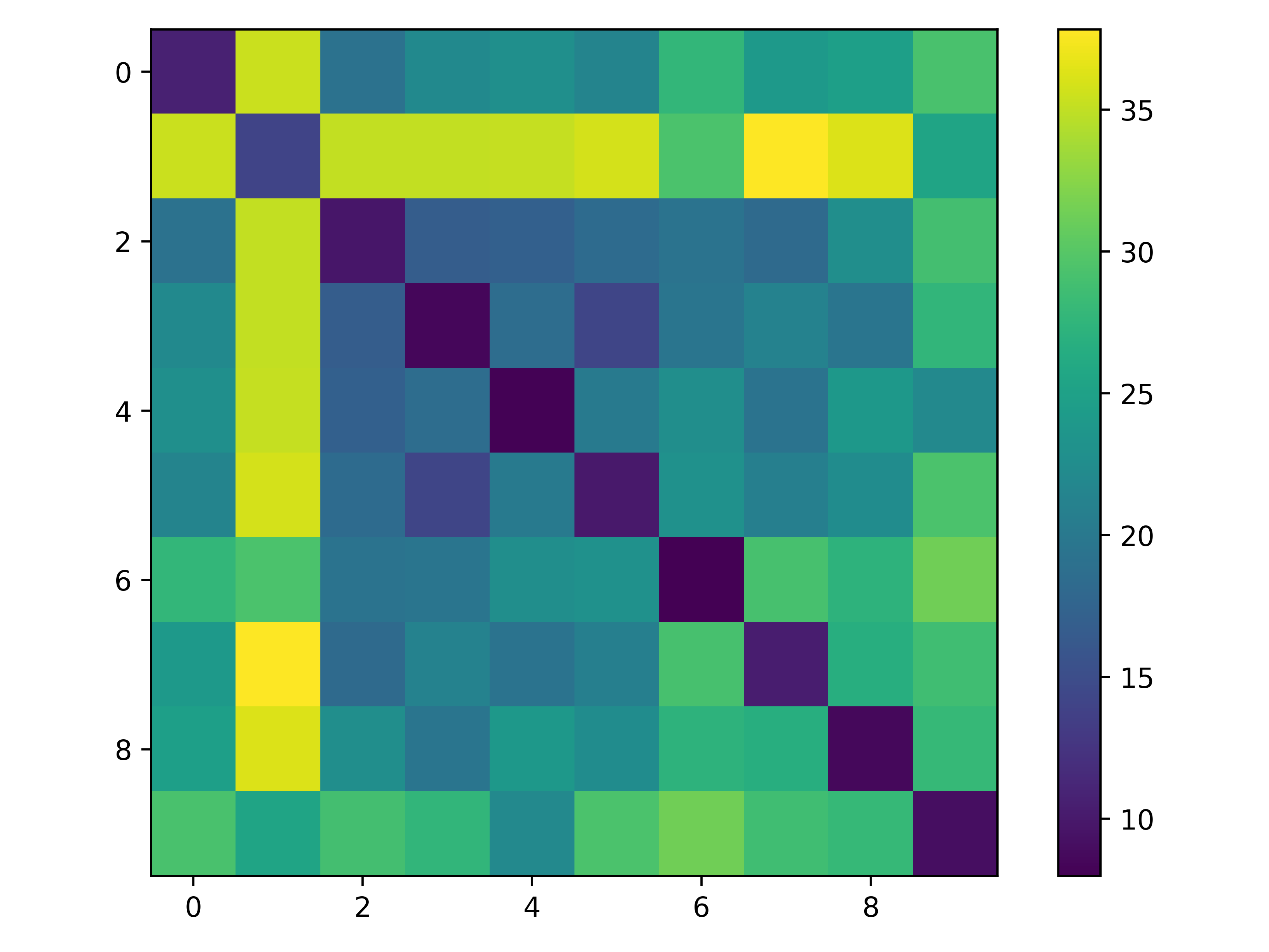
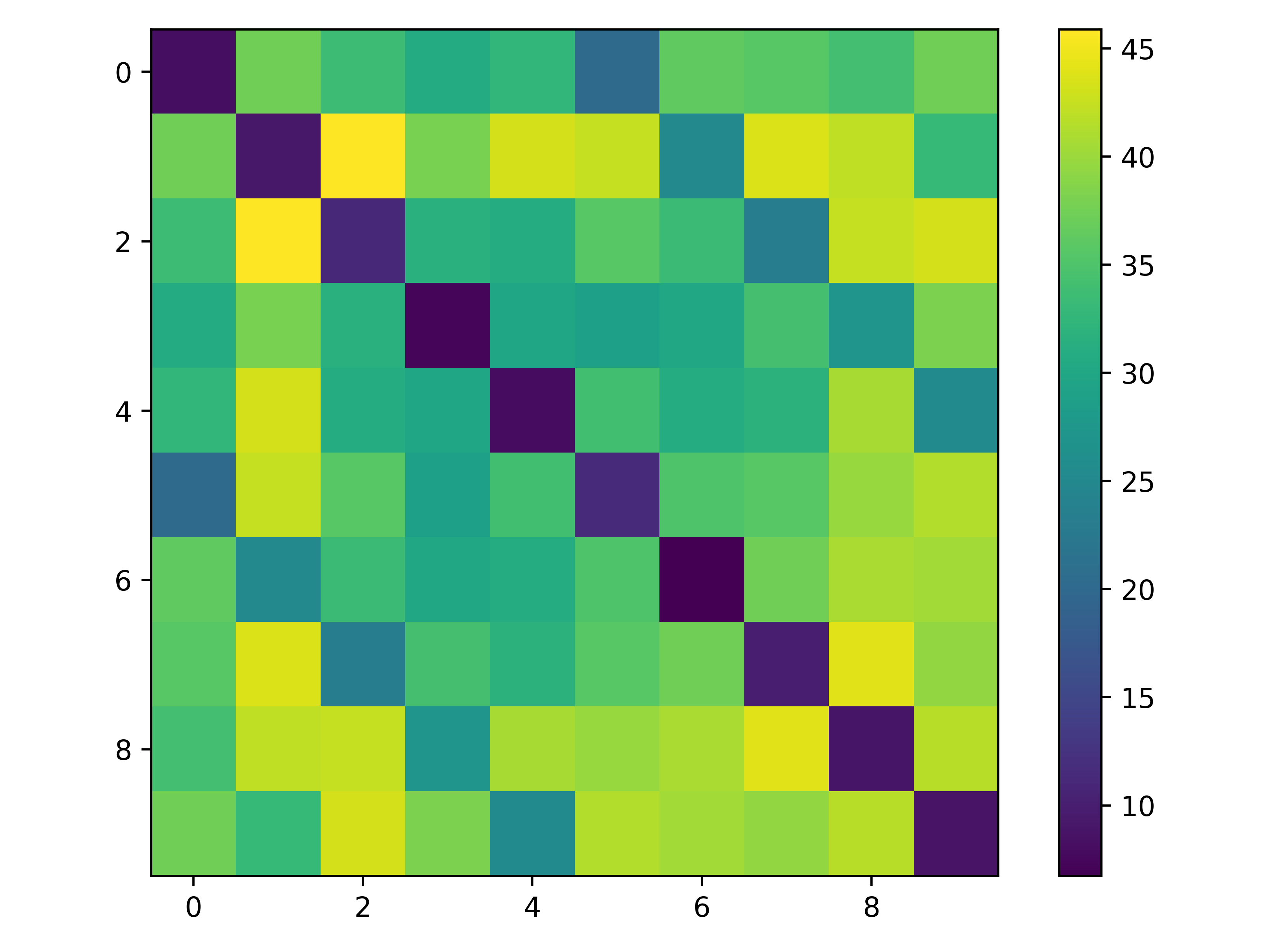
Since the model is trained on the coarse dataset, Neural Collapse asserts that for every original class pair i,j𝑖𝑗i,j in the same super-class (including the case of i=j𝑖𝑗i=j), the class distance Di,jsubscript𝐷𝑖𝑗D_{i,j} should be very small. In Coarse CIFAR-10, this will result in three darks lines (darker color represents lower value) in the heatmap of D𝐷D since each super class contains two original classes, as illustrated in Figure 4 (b). For example, in Coarse CIFAR-10 the original class "airplane" and "dog" both belong to the super class "airplane & dog", therefore per Neural Collapse’s prediction, their last-layer representations would collapse to each other, making the average square distance extremely small compared to other entries. In contrast, if the last-layer representations perfectly reflect the distribution of input, i.e. original classes, the class distance matrix should be a diagonal matrix as shown in Figure 4 (a), because the last-layer representation of samples in each original class only collapse to the class-mean of this original class.

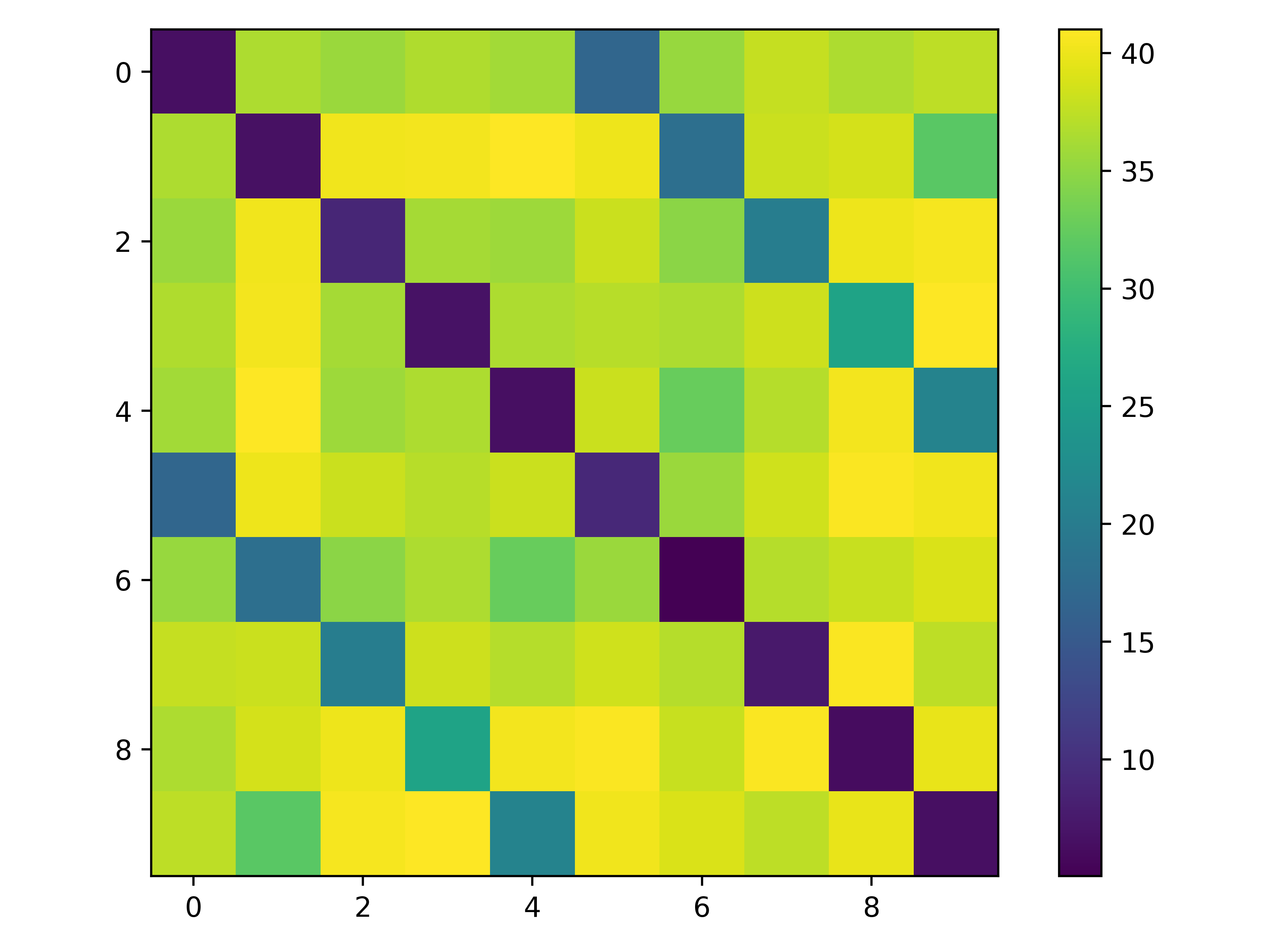
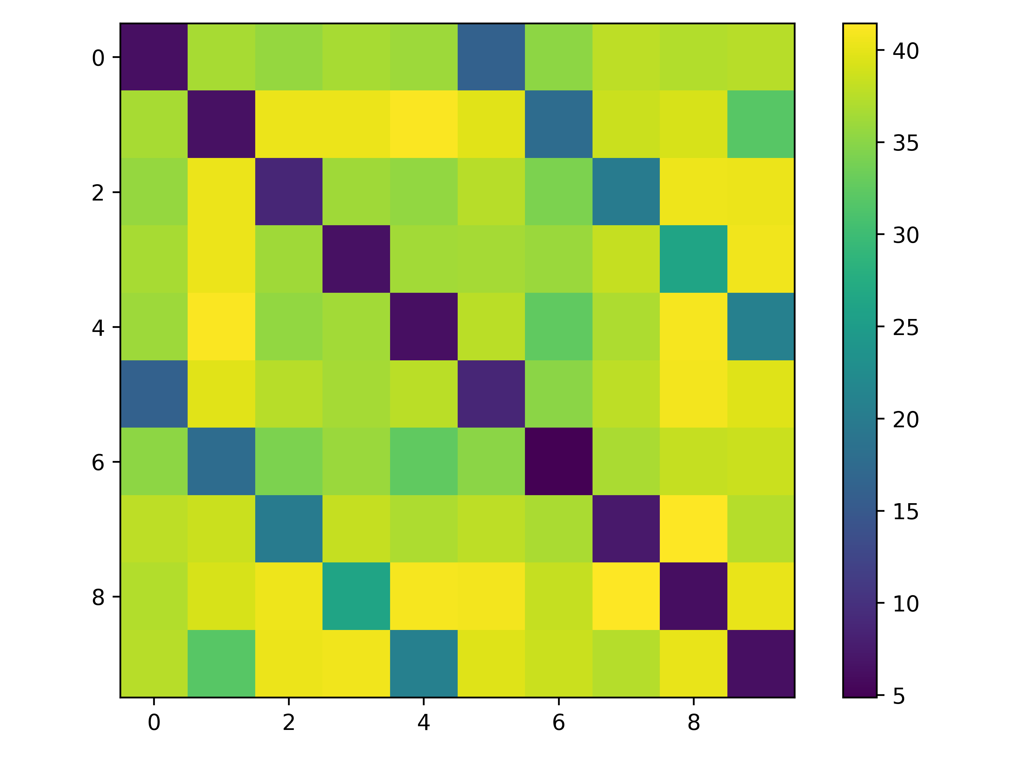
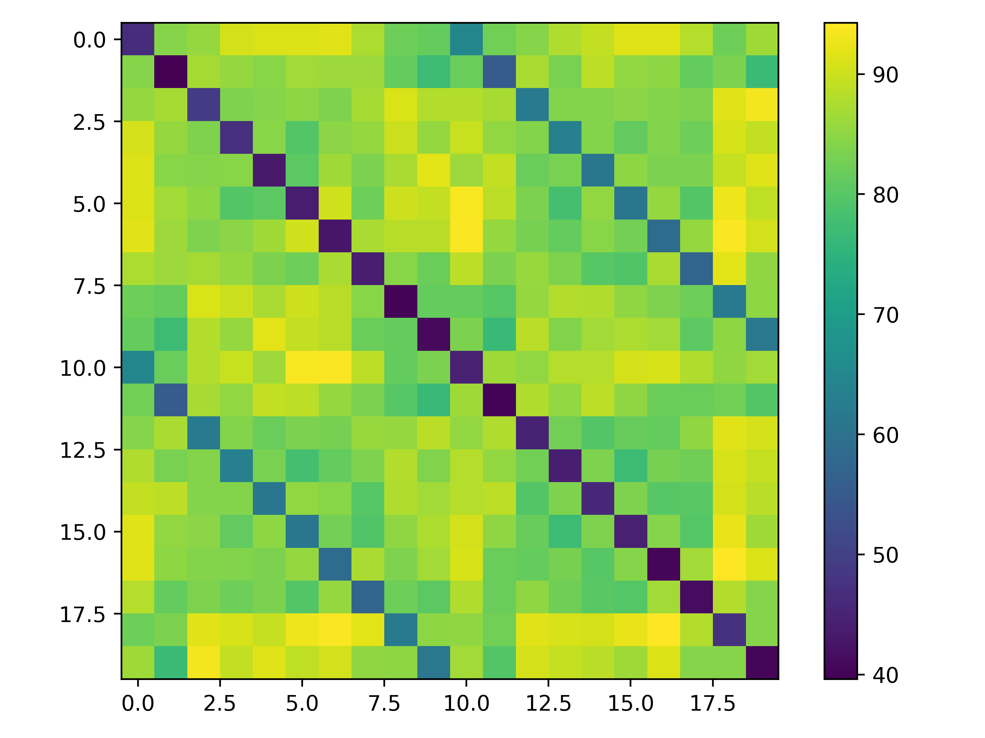
Figure 5 displays the heatmaps of class distance matrix D𝐷D at different stages in training, which shows that: (i) There are indeed three dark lines that show up, but they do not show up simultaneously. In particular, the central diagonal line – representing the samples in the same original classes – emerges earlier in training. (ii) Even in the final stage of training when the training error is zero, the three lines are not of the same degree of darkness. The central line is clearly darker, indicating a smaller distance within the original classes.

Those observations suggest that the actual behaviour of the last-layer representations is between the cases predicted in Figure 4 (a) and (b): the input distribution and training labels both have an impact on the distribution of the last-layer representations, both of them can be present even after reaching zero training error for a long time, and the impact of input distribution emerges earlier in training. These observations suggest both the existence of Neural Collapse and the inadequacy of Neural Collapse to completely describe the behaviour of last-layer representations.
Refer to caption
(a) epoch = 20
Refer to caption
(b) epoch = 120
Refer to caption
(c) epoch = 240
Refer to caption
(d) epoch = 350
Figure 5: The heatmap of class distance matrix.

4.2 Visualization

In this subsection, we take a closer look at the last-layer representations of the model at the end of training by reducing the dimensionality of the last-layer representations to 222 through t-SNE (Van der Maaten & Hinton, 2008) and visualize them. Specifically, we visualize each super-class separately, but color the samples whose original labels are different with different colors.

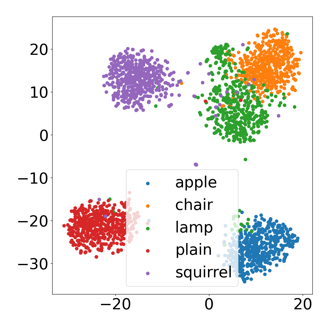
The visualization results are displayed in Figure 6, from which we observe a distinguishable difference between different original classes — their representations form well-separated clusters in the 2-dimensional space. This suggests that the input distribution information, i.e. the original label information, is well preserved in the last-layer representations.

Refer to caption
Figure 6: The t-SNE visualization of the last-layer representations of ResNet-18 trained on Coarse CIFAR-10. Each plot corresponds to a super-class.

Training extremely long.

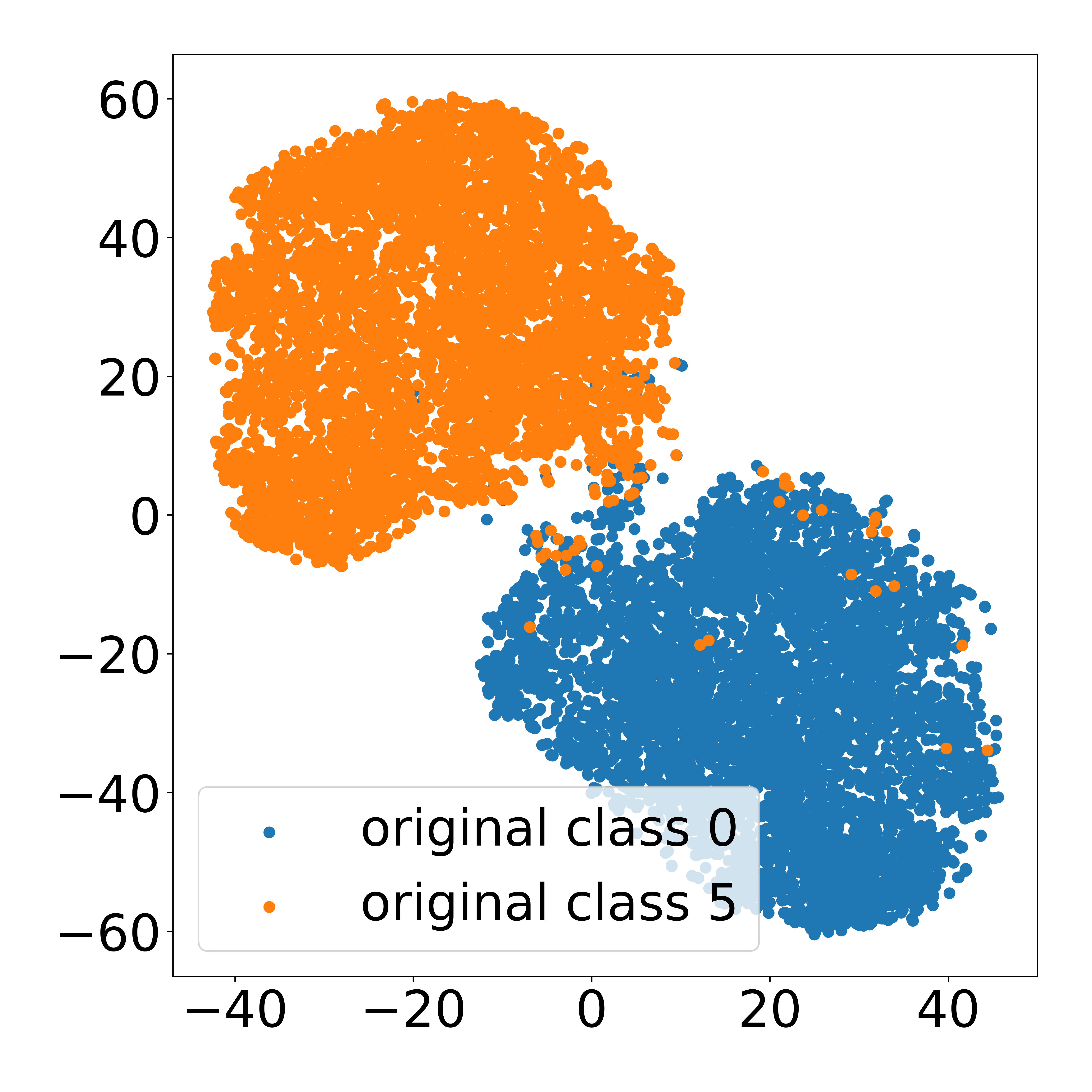
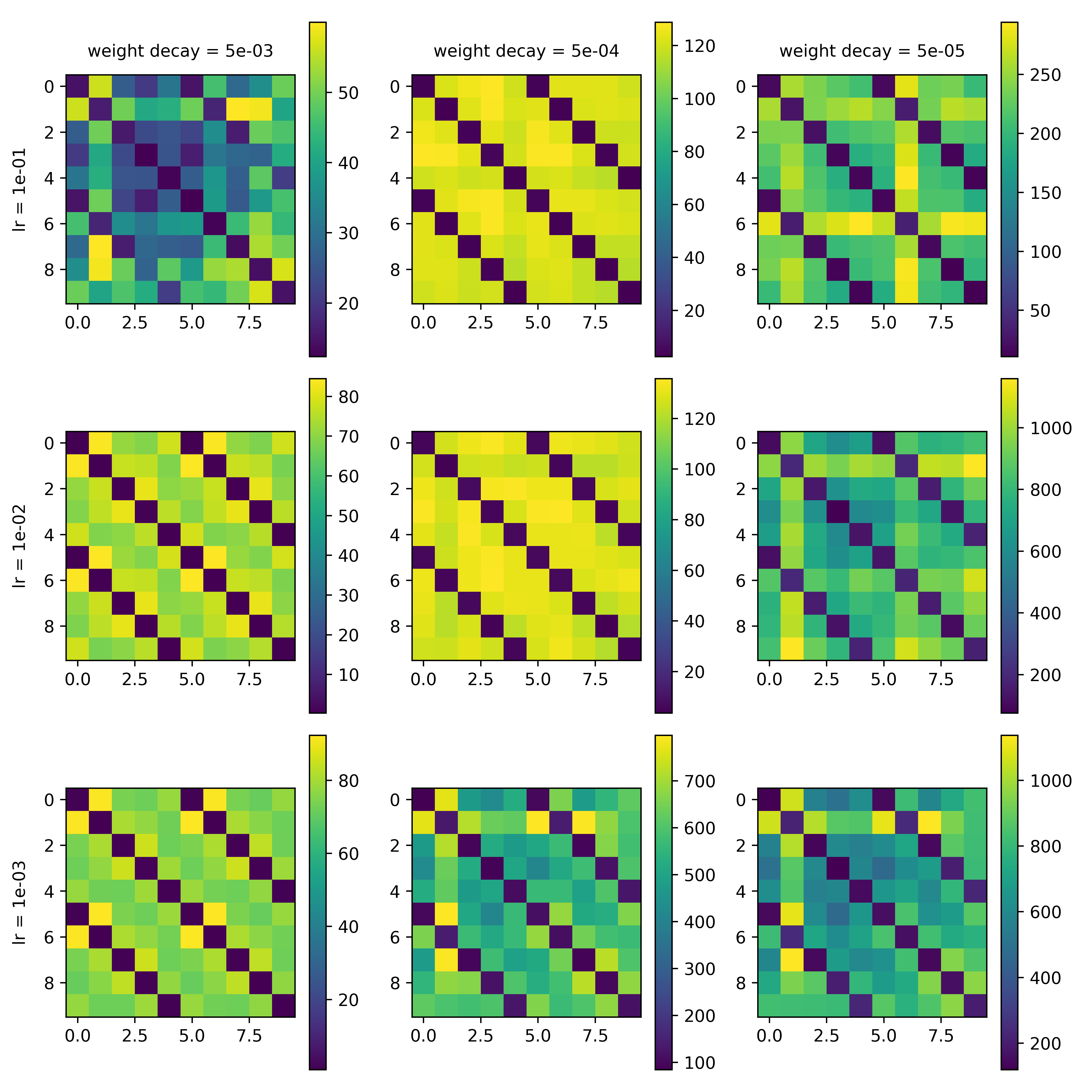
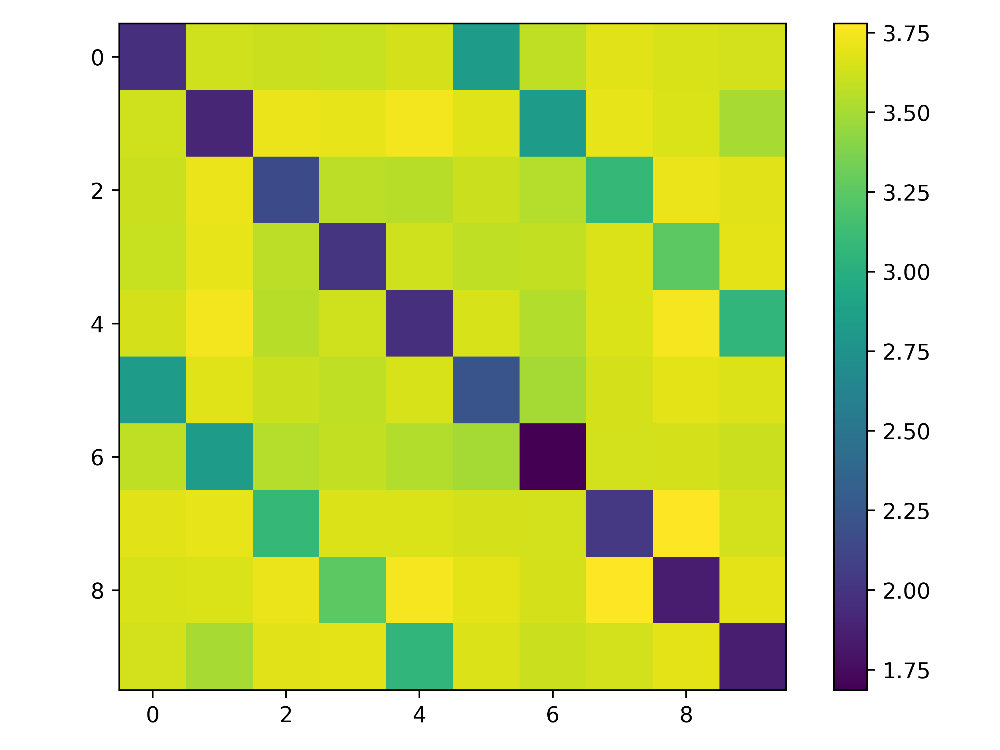
In order to explore if the fine-grained structures are still preserved even after a extremely long time of training, we further train the model with 1,000 epochs. The heatmap of the distance matrix is presented in Figure 8. We also produce the t-SNE visualizations, but only include the result of the first super-class in Figure 8 due to space limitation.
Refer to caption
Figure 7: The heatmap of distance matrix of ResNet-18 trained on Coarse CIFAR-10 for 1,000 epochs.
Refer to caption
Figure 8: The t-SNE visualization of the last-layer representations of the first super-class of ResNet-18 trained on Coarse CIFAR-10 for 1,000 epochs.

4.3 Learning CIFAR-10 from 5 Coarse Labels

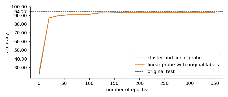
As the results in Section 4.2 suggest, even after the training accuracy has reached 100%percent100100\% for a long time, the samples within each super-class still exhibit a clear structure per their original class, and those structures act as clusters after reducing dimensionality. Inspired by this observation, we perform a Cluster-and-Linear-Probe (CLP) test to quantify to what extent the original class information is preserved in the last-layer representations. In CLP, we use the representations learned on Coarse CIFAR-10 to reconstruct 101010 labels and run a linear probe on these representations using the reconstructed labels. Specifically, we first use t-SNE to reduce the dimensionality to 222 and then use k𝑘k-means to find 222 clusters in the dimensionality-reduced representations within each super-class. We use the clusters as reconstructed labels to do a linear probe. In linear probe, we train a linear classifier on top of the previously learned representations on the training set with reconstructed labels and evaluate the learned linear classifier on the original test set. Notice that because we do not know the mapping of reconstructed classes to true original classes, we permute each possible mapping and report the highest performance. We also train a linear probe with original training labels as a comparison. The result is shown in Figure 9.

The performance of CLP on the original test set is comparable to linear probe trained on true original labels or even to models originally trained on CIFAR-10. Notice that the representation H𝐻H is obtained from the model trained with coarse labels, and the label reconstruction only uses information of H𝐻H and the number of original classes. This means we can achieve very high performance on the original test set even if we only have access to coarse labels. This result further confirms that the input distribution plays an important role in the last-layer representations.
Refer to caption
Figure 9: The CLP result. “original test” is the highest test set accuracy achieved by ResNet18 trained on original CIFAR-10 with the same training hyper-parameters.

5 How Does Semantic Similarity Affect the Fine-Grained Structure?

In our experiments with Coarse CIFAR-10, each coarse label is obtained by combining two classes regardless of the semantics. The fact that the neural network can separate the two classes in its representation space implies that the network recognizes these two classes as semantically different (even though they are given the same coarse label). In this section, we explore the following question: If the sub-classes in a super-class have semantic similarity, will the representations still exhibit a fine-grained structure to distinguish them? Intuitively, if the coarse label provided is “natural” and consists of semantically similar sub-classes, it is possible that the neural network will not distinguish between them and just produce truly collapsed representations.
Refer to caption
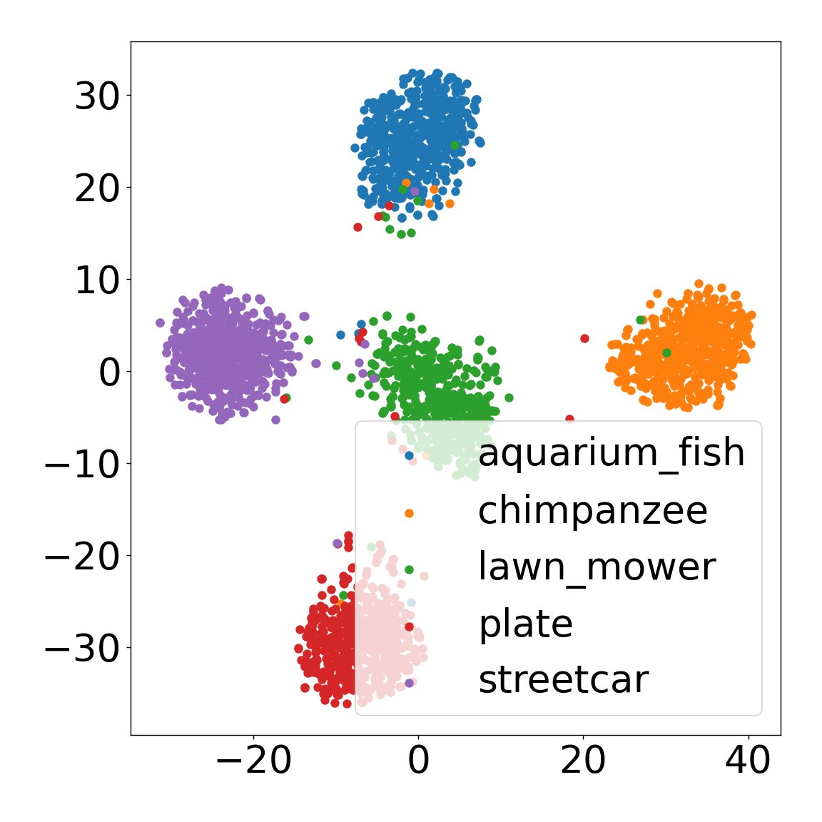
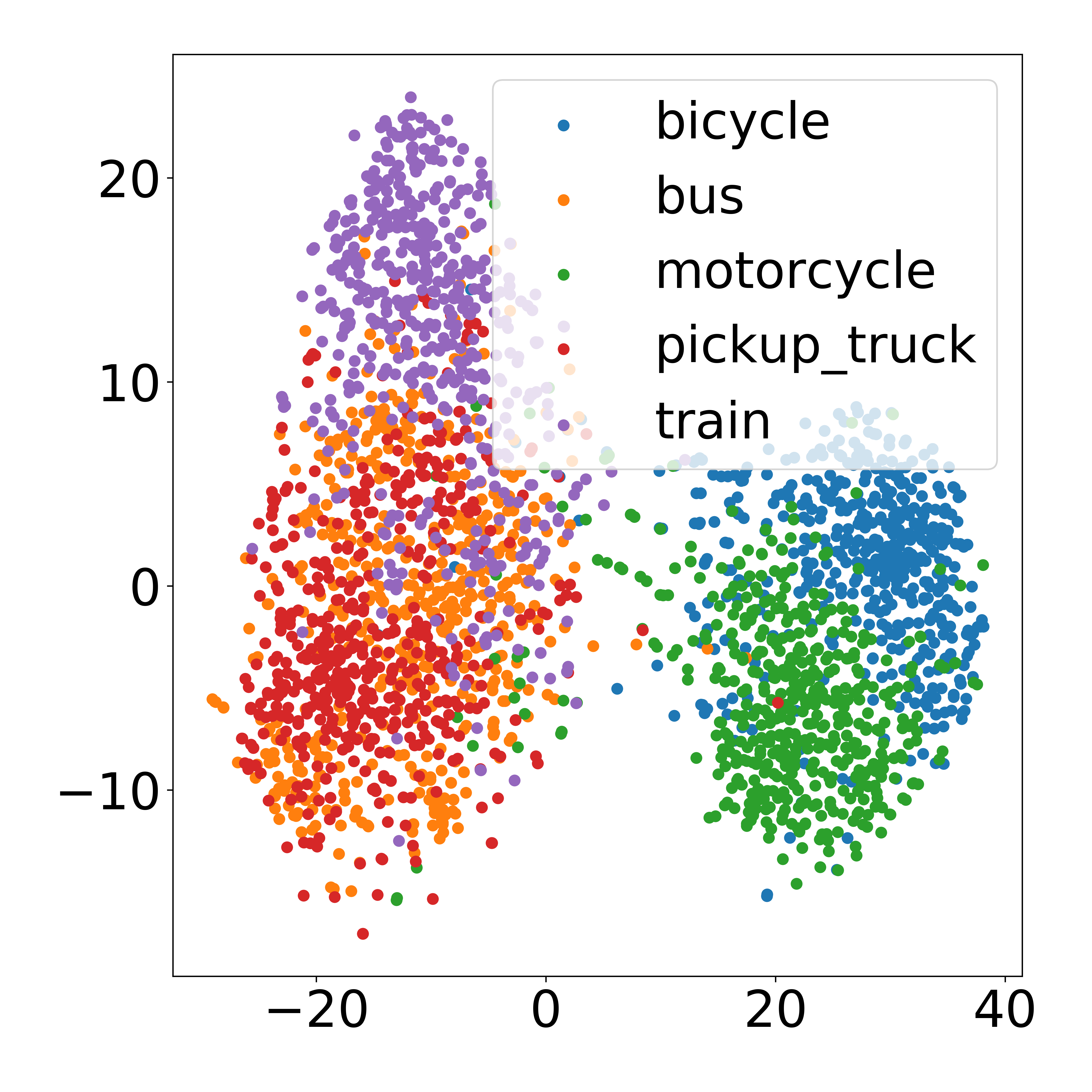
Figure 10: The t-SNE visualization of the last-layer representations of super-class “vehicles 1” of ResNet-18 trained on CIFAR-100 with original super-classes.
Refer to caption
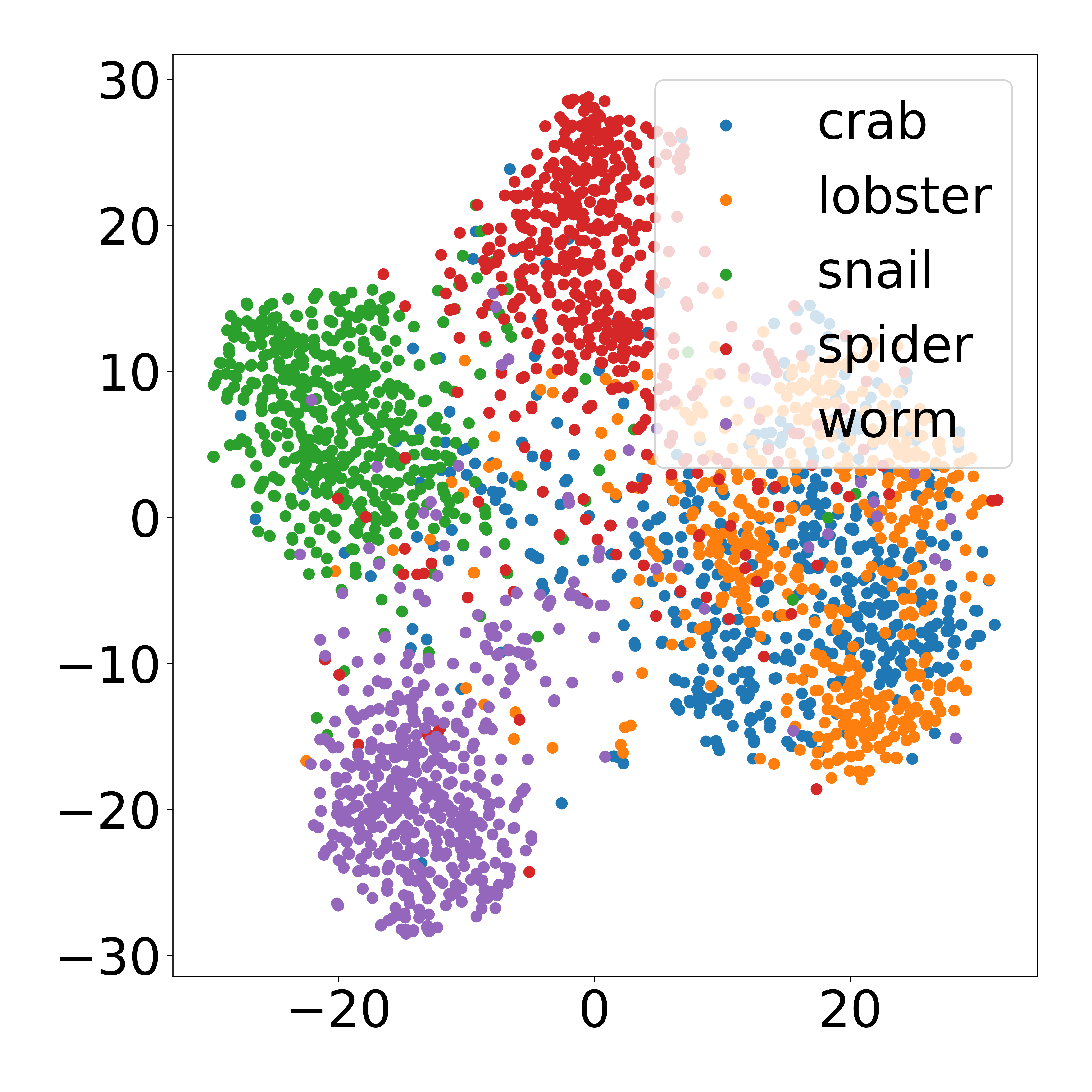
Figure 11: The t-SNE visualization of the last-layer representations of super-class “non-insect invertebrates” of ResNet-18 trained on CIFAR-100 with original super-classes.
Refer to caption
Figure 12: The t-SNE visualization of the last-layer representations of super-class 1 of ResNet-18 trained on CIFAR-100 with random super-classes.
Refer to caption
Figure 13: The t-SNE visualization of the last-layer representations of super-class 2 of ResNet-18 trained on CIFAR-100 with random super-classes.

We take a step towards answering this question by looking at ResNet-18 trained on CIFAR-100 using the official 20 super-classes (each super-class contains 5 sub-classes) as labels. Unlike randomly merging classes as we did in Section 4, the official super-classes of CIFAR-100 are natural, merging classes with similar semantics (for example, “beaver” and “dolphin” both belong to “aquatic mammals”). This offers a perfect testbed for our question.

We find that ResNet-18 indeed is not able to distinguish all sub-classes in its representation space, but can still produce separable representations if some sub-classes within a super-class are sufficiently different. Interestingly, the notion of semantic similarity of ResNet-18 turns out to agree well with that of humans. Figures 11 and 11 show the t-SNE visualizations of representations from two super-classes. From the visualizations, although there are not as clear clusters as for Coarse CIFAR-10, the representations do exhibit visible separations between certain sub-classes. In Figure 11, “bicycles” and “motorcycles” are entangled together, while they are separated from “bus”, “pickup truck”, and “train”, which is human-interpretable. In Figure 11, “crab” and “lobster” are mixed together, which are both aquatic and belong to malacostraca, while the other three are not and have more differentiative representations.

In comparison, when the CIFAR-100 classes are randomly merged into 20 super-classes, we find that the sub-class representations are much better separated (Figures 13 and 13). This is because randomly merged super-classes no longer have semantic similarity in their sub-classes.

These results confirm the intuition that the fine-grained structure in last-layer representations is affected by, or even based on, the semantic similarity between the inputs.

6 Fine-Grained Representation Structure on Fine CIFAR-10

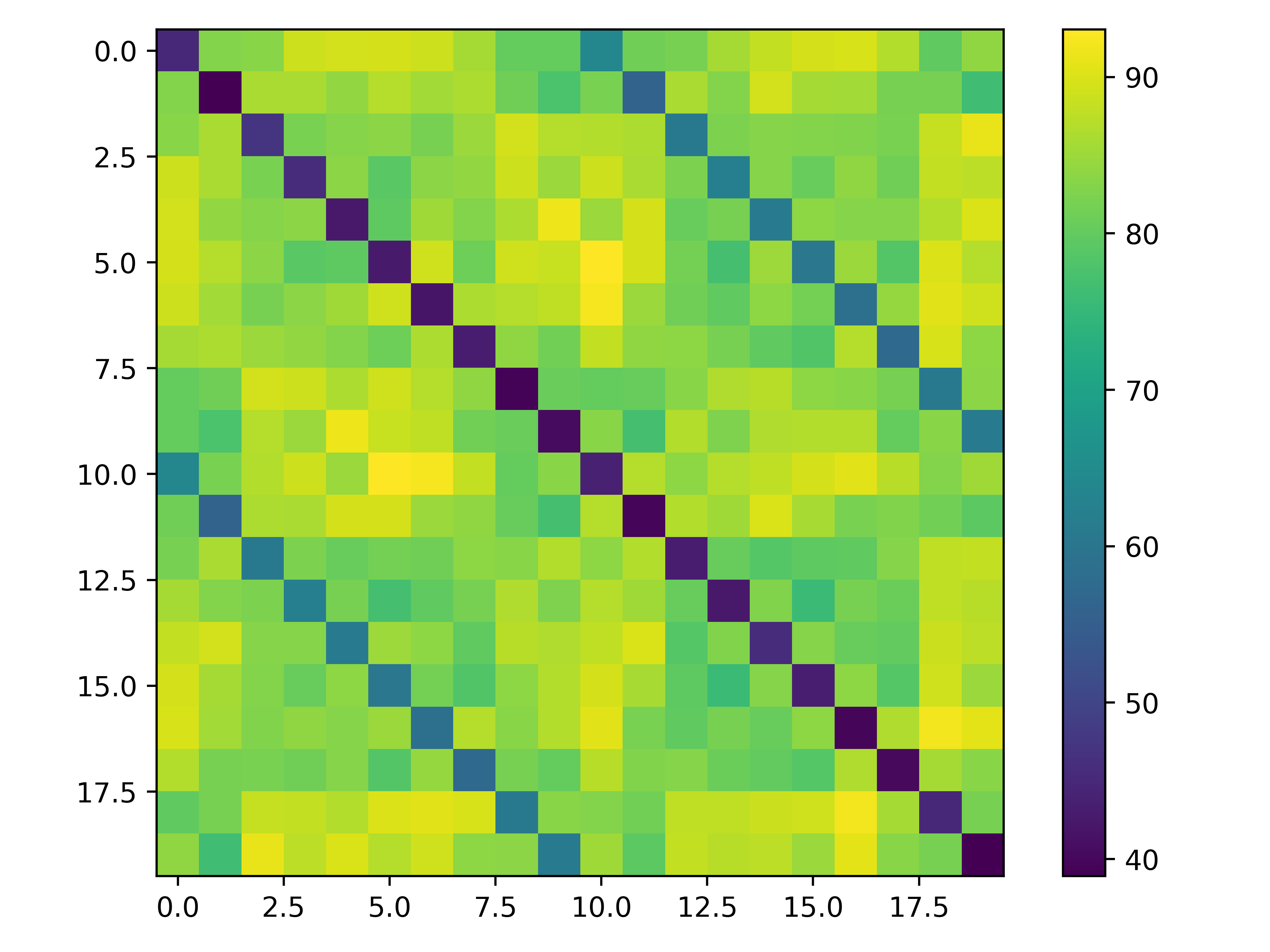
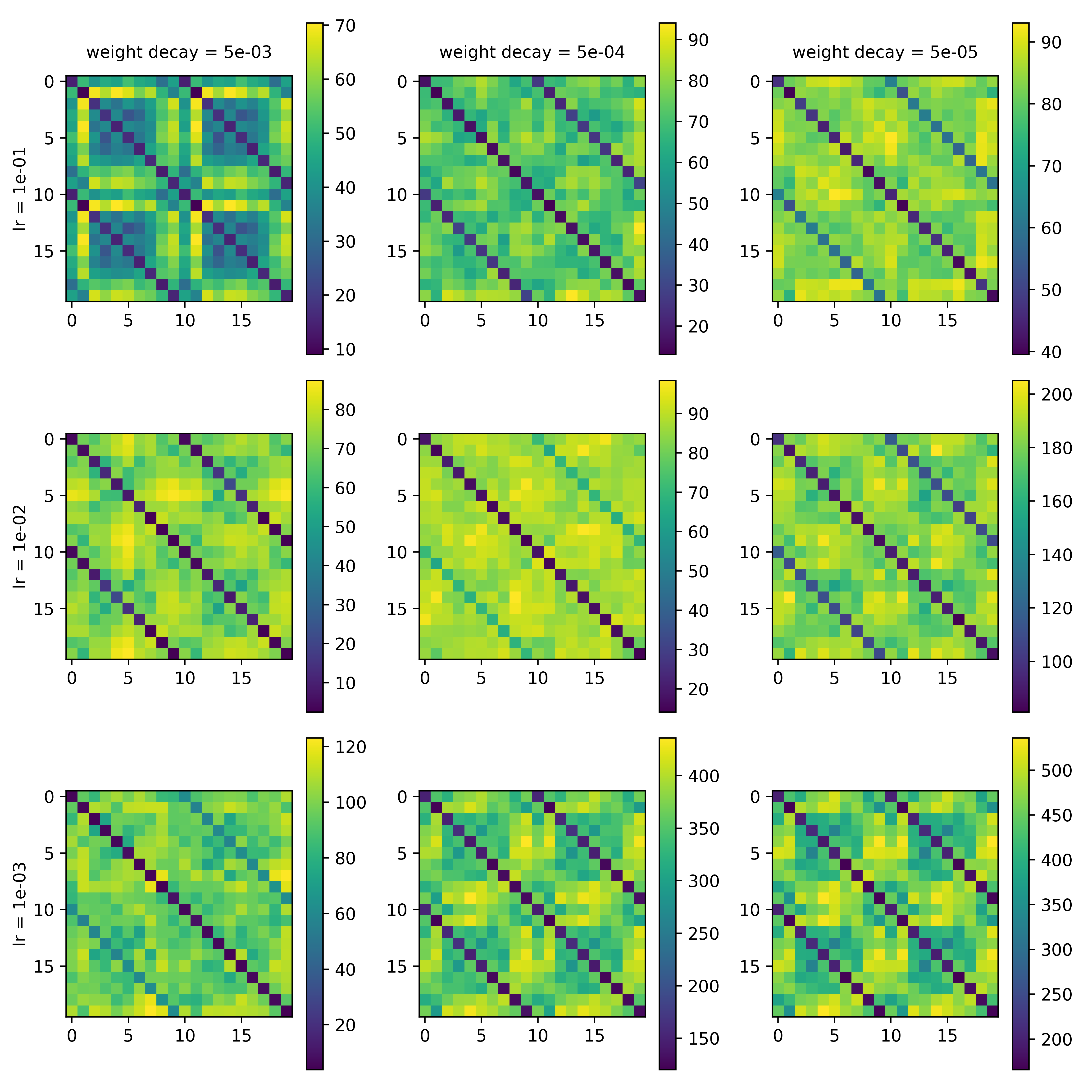
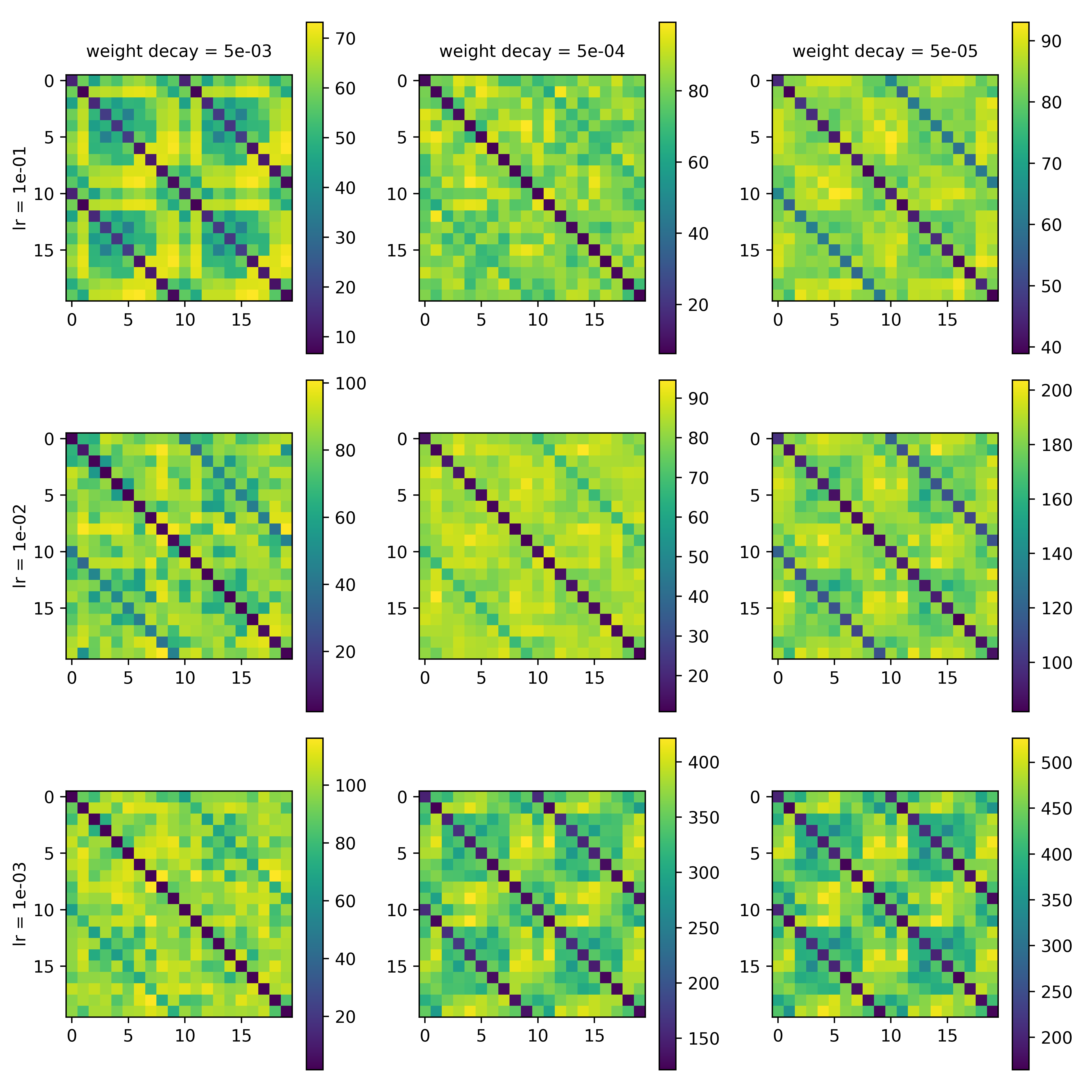
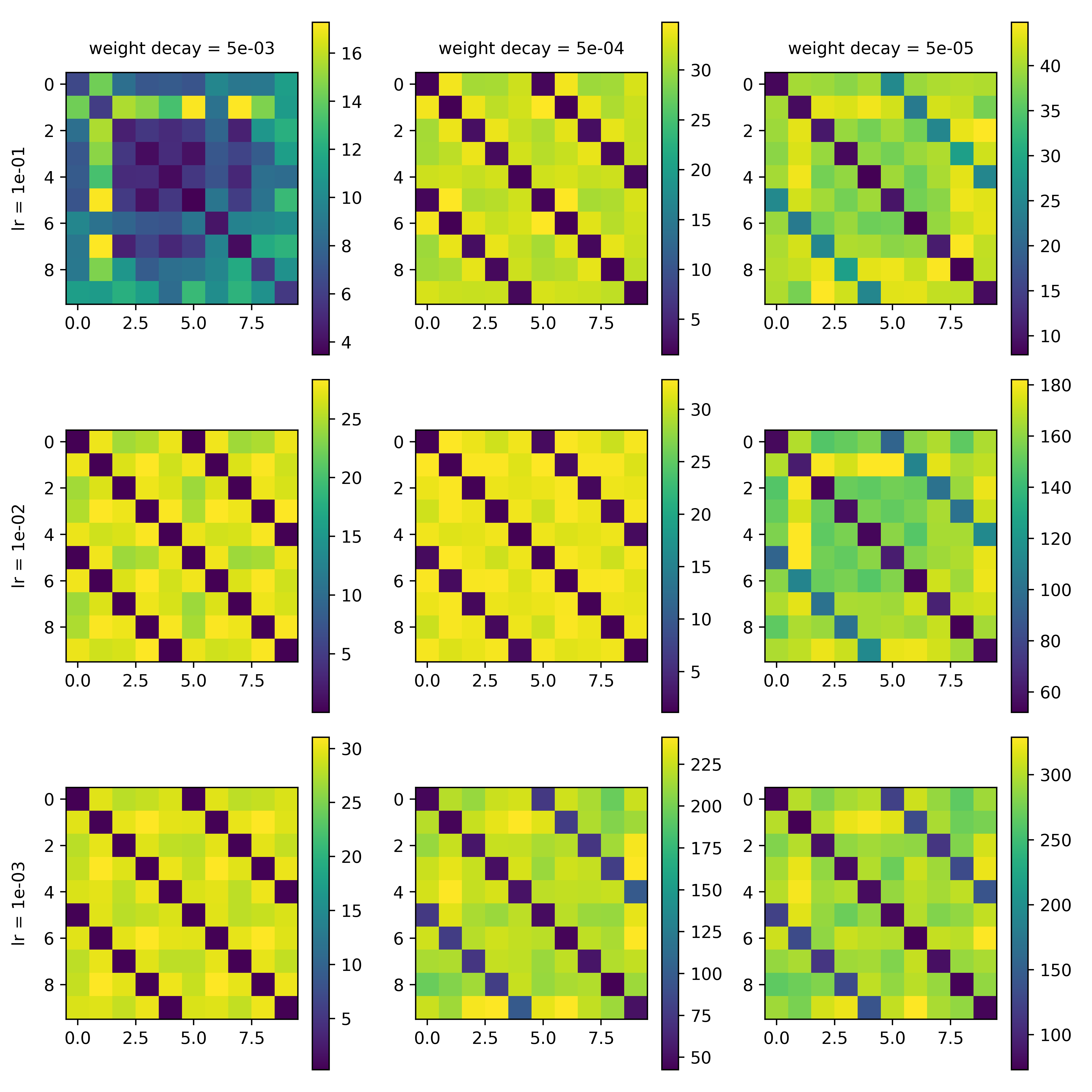
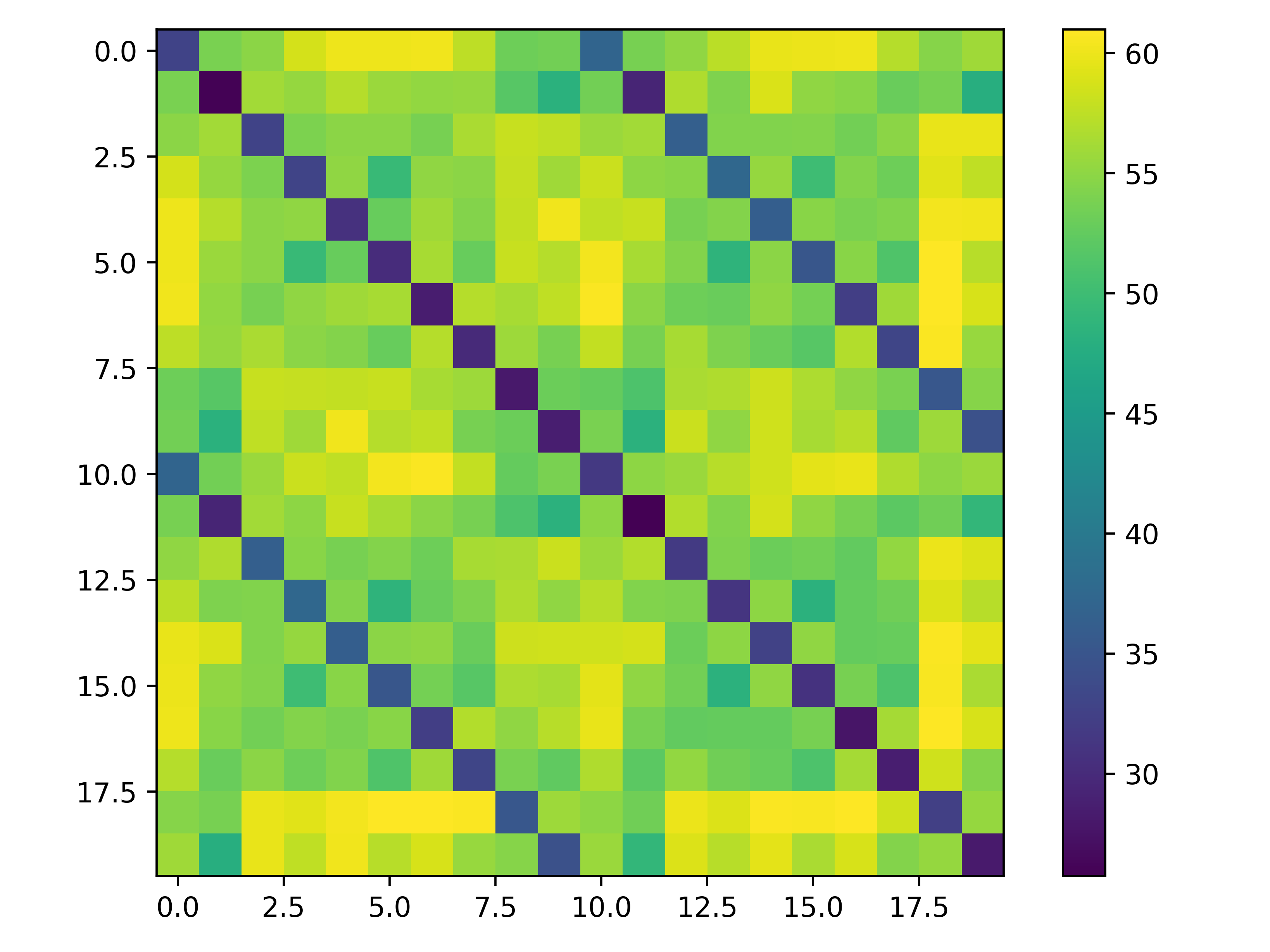
In this section, we consider a finely-labeled dataset. We construct a fine version of CIFAR-10 with the process described in Section 3.2, and call it Fine CIFAR-10. Figure 14 presents the class distance matrices, arranged by the number of training epochs. As before, we only provide the results for a specific training hyper-parameter setting here and defer the full results to Appendix D.

It can be observed that at the early stage of training, there are three dark lines, which indicates the last-layer representations are converging towards 101010 clusters instead of 202020. At the end of training, this 101010-class relationship is still preserved, although with a lighter color. Therefore, both the input distribution and the label information still have a strong influence on the representation structure when fine labels are used for training.
Refer to caption
(a) epoch = 20
Refer to caption
(b) epoch = 120
Refer to caption
(c) epoch = 240
Refer to caption
(d) epoch = 350
Figure 14: The heatmap of class distance matrix on Fine CIFAR-10.

7 Theoretical Result in a Synthetic Setting

In this section, we provide a theoretical result to show the fine-grained representation structure for a coarsely labeled dataset, supporting our empirical observations in previous sections. In particular, we consider a one-hidden-layer neural network trained by gradient descent on Gaussian mixture data. We describe our setting below.

Data generation.

We consider input data generated from a mixture of 4 separated Gaussian distributions in dsuperscript𝑑\mathbb{R}^{d}. We denote the four clusters as 𝒞1subscript𝒞1\mathscr{C}_{1}, 𝒞2subscript𝒞2\mathscr{C}_{2}, 𝒞3subscript𝒞3\mathscr{C}_{3}, and 𝒞4subscript𝒞4\mathscr{C}_{4}. We give coarse label +11+1 to inputs from 𝒞1subscript𝒞1\mathscr{C}_{1} and 𝒞2subscript𝒞2\mathscr{C}_{2}, and give coarse label 11-1 to inputs from 𝒞3subscript𝒞3\mathscr{C}_{3} and 𝒞4subscript𝒞4\mathscr{C}_{4}. We denote the n𝑛n samples as {(𝒙i,yi)}i=1nsuperscriptsubscriptsubscript𝒙𝑖subscript𝑦𝑖𝑖1𝑛\{(\boldsymbol{x}_{i},y_{i})\}_{i=1}^{n}. We assume a sample 𝒙isubscript𝒙𝑖{\boldsymbol{x}}_{i} where i𝒞p𝑖subscript𝒞𝑝i\in\mathscr{C}_{p} (p{1,2,3,4}𝑝1234p\in\{1,2,3,4\}) is generated according to

𝒙i=𝝁(p)+𝝃i,subscript𝒙𝑖superscript𝝁𝑝subscript𝝃𝑖{\boldsymbol{x}}_{i}={\boldsymbol{\mu}}^{(p)}+{\boldsymbol{\xi}}_{i}, (7)

where 𝝃i𝒩(0,κ2𝑰)similar-tosubscript𝝃𝑖𝒩0superscript𝜅2𝑰{\boldsymbol{\xi}}_{i}\sim\mathcal{N}(0,\kappa^{2}{\boldsymbol{I}}). We assume that the means 𝝁(p)superscript𝝁𝑝{\boldsymbol{\mu}}^{(p)}’s are pairwise orthogonal and 𝝁(p)2=τsubscriptnormsuperscript𝝁𝑝2𝜏\|{\boldsymbol{\mu}}^{(p)}\|_{2}=\tau. For convenience, assume each cluster 𝒞psubscript𝒞𝑝\mathscr{C}_{p} has the same number of samples |𝒞p|=n/4subscript𝒞𝑝𝑛4|\mathscr{C}_{p}|=n/4.

Neural network.

We consider training a one-hidden-layer network with m𝑚m hidden neurons. The first-layer weight matrix is W=(𝒘1,𝒘2,,𝒘m)d×m𝑊subscript𝒘1subscript𝒘2subscript𝒘𝑚superscript𝑑𝑚W=({\boldsymbol{w}}_{1},{\boldsymbol{w}}_{2},\cdots,{\boldsymbol{w}}_{m})\in\mathbb{R}^{d\times m} and is trained by gradient descent. The second-layer weights are fixed to be all ones (which satisfies the ETF structure predicted by Neural Collapse in this setting). The output of the network is

f(𝒙,W)=𝟏h(𝒙,W)=r=1mσ(𝒘r𝒙),𝑓𝒙𝑊superscript1top𝒙𝑊superscriptsubscript𝑟1𝑚𝜎superscriptsubscript𝒘𝑟top𝒙f({\boldsymbol{x}},W)=\mathbf{1}^{\top}h({\boldsymbol{x}},W)=\sum_{r=1}^{m}\sigma\left({\boldsymbol{w}}_{r}^{\top}\boldsymbol{x}\right),

where h(𝒙,W)=(σ(𝒘r𝒙))r=1mm𝒙𝑊superscriptsubscript𝜎superscriptsubscript𝒘𝑟top𝒙𝑟1𝑚superscript𝑚h(\boldsymbol{x},W)=\left(\sigma({\boldsymbol{w}}_{r}^{\top}\boldsymbol{x})\right)_{r=1}^{m}\in\mathbb{R}^{m} is the hidden-layer representation, and

σ(z)={13z3if |z|1z23if z1z+23if z1𝜎𝑧cases13superscript𝑧3if |z|1𝑧23if z1𝑧23if z1\sigma(z)=\begin{cases}\frac{1}{3}z^{3}&\text{if $|z|\leq 1$}\\ z-\frac{2}{3}&\text{if $z\geq 1$}\\ z+\frac{2}{3}&\text{if $z\leq-1$}\end{cases}

is the activation function. This activation is a smoothed version of symmetrized ReLU; it and its variants have been adopted in a line of theoretical work (e.g. Allen-Zhu & Li (2020); Zou et al. (2021); Shen et al. (2022)).

Loss function and training algorithm.

We train the network by gradient descent on the training loss

L(W)=1ni=1n(f(𝒙i,W),yi)𝐿𝑊1𝑛superscriptsubscript𝑖1𝑛𝑓subscript𝒙𝑖𝑊subscript𝑦𝑖L(W)=\frac{1}{n}\sum_{i=1}^{n}\ell(f({\boldsymbol{x}}_{i},W),y_{i})

where (y^,y)=yy^2^𝑦𝑦𝑦^𝑦2\ell(\hat{y},y)=\frac{-y\hat{y}}{2} is the unhinged loss (van Rooyen et al., 2015). Our result can be generalized to the logistic loss since when f(𝒙i,W)𝑓subscript𝒙𝑖𝑊f({\boldsymbol{x}}_{i},W) is small, the unhinged loss can be viewed as an approximation of logistic loss (Shen et al., 2022). We initialize the first-layer weights i.i.d. from 𝒩(0,ω2)𝒩0superscript𝜔2\mathcal{N}(0,\omega^{2}) and update them using gradient descent with learning rate η𝜂\eta.

Our main theorem shows that after training, the hidden-layer representations for 𝒞1subscript𝒞1\mathscr{C}_{1} and 𝒞2subscript𝒞2\mathscr{C}_{2} will form two separate clusters, even though they are given the same label. (Similar result holds for 𝒞3subscript𝒞3\mathscr{C}_{3} and 𝒞4subscript𝒞4\mathscr{C}_{4} by symmetry.) In particular, for any three samples i1,i2𝒞1subscript𝑖1subscript𝑖2subscript𝒞1i_{1},{i_{2}}\in\mathscr{C}_{1} and i3𝒞2subscript𝑖3subscript𝒞2{i_{3}}\in\mathscr{C}_{2}, we show that

h(𝒙i1)h(𝒙i2)2h(𝒙i1)h(𝒙i3)2.much-less-thansubscriptnormsubscript𝒙subscript𝑖1subscript𝒙subscript𝑖22subscriptnormsubscript𝒙subscript𝑖1subscript𝒙subscript𝑖32\left\|h({\boldsymbol{x}}_{i_{1}})-h({\boldsymbol{x}}_{i_{2}})\right\|_{2}\ll\|h({\boldsymbol{x}}_{i_{1}})-h({\boldsymbol{x}}_{i_{3}})\|_{2}.
Theorem 7.1.

Consider the synthetic setting describe above and let 𝔠=8κdτ𝔠8𝜅𝑑𝜏\mathfrak{c}=\frac{8\kappa\sqrt{d}}{\tau}. Suppose that the following conditions hold regarding the Gaussian mean length τ𝜏\tau, Gaussian variance κ2superscript𝜅2\kappa^{2}, weight initialization variance ω2superscript𝜔2\omega^{2}, input dimension d𝑑d, number of samples n𝑛n, and number of neurons m𝑚m:

  1. 1.

    n12d14𝔠n12d16much-less-thansuperscript𝑛12superscript𝑑14𝔠much-less-thansuperscript𝑛12superscript𝑑16n^{\frac{1}{2}}d^{-\frac{1}{4}}\ll\mathfrak{c}\ll n^{\frac{1}{2}}d^{-\frac{1}{6}};

  2. 2.

    d1/3nmuch-greater-thansuperscript𝑑13𝑛d^{1/3}\gg n;

  3. 3.

    d14n12𝔠1τωlog12(m)much-less-thansuperscript𝑑14superscript𝑛12superscript𝔠1𝜏𝜔much-less-thansuperscript12𝑚d^{-\frac{1}{4}}n^{\frac{1}{2}}\mathfrak{c}^{-1}\ll\tau\omega\ll\log^{-\tfrac{1}{2}}(m).

For learning rate η=O(min{𝔠3τ4,𝔠2ωτ3,𝔠2ωτ})𝜂𝑂superscript𝔠3superscript𝜏4superscript𝔠2𝜔superscript𝜏3superscript𝔠2𝜔𝜏\eta=O\left(\min\left\{\mathfrak{c}^{3}\tau^{-4},\mathfrak{c}^{2}\omega\tau^{-3},\mathfrak{c}^{2}\omega\tau\right\}\right) and number of iterations T=Θ(1ηωτ3)𝑇Θ1𝜂𝜔superscript𝜏3T=\Theta(\frac{1}{\eta\omega\tau^{3}}), with high probability, the hidden-layer representation map h(𝐱)=h(𝐱,W(T))𝐱𝐱𝑊𝑇h(\boldsymbol{x})=h(\boldsymbol{x},W(T)) satisfies that for all i1,i2𝒞1subscript𝑖1subscript𝑖2subscript𝒞1i_{1},{i_{2}}\in\mathscr{C}_{1} and i3𝒞2subscript𝑖3subscript𝒞2{i_{3}}\in\mathscr{C}_{2}, we have

h(𝒙i1)h(𝒙i2)2h(𝒙i1)h(𝒙i3)2.much-less-thansubscriptnormsubscript𝒙subscript𝑖1subscript𝒙subscript𝑖22subscriptnormsubscript𝒙subscript𝑖1subscript𝒙subscript𝑖32\left\|h({\boldsymbol{x}}_{i_{1}})-h({\boldsymbol{x}}_{i_{2}})\right\|_{2}\ll\|h({\boldsymbol{x}}_{i_{1}})-h({\boldsymbol{x}}_{i_{3}})\|_{2}.

An example set of parameters that satisfy the above conditions is:

κ=1,τ=d0.52,ω=d0.53,m=logd,n=d0.32.formulae-sequence𝜅1formulae-sequence𝜏superscript𝑑0.52formulae-sequence𝜔superscript𝑑0.53formulae-sequence𝑚𝑑𝑛superscript𝑑0.32\displaystyle\kappa=1,\tau=d^{0.52},\omega=d^{-0.53},m=\log d,n=d^{0.32}.

The proof of Theorem 7.1 is given in Appendix A. The main step is to prove that after training, the neurons 𝒘rsubscript𝒘𝑟\boldsymbol{w}_{r} will be better correlated with the class means 𝝁(p)superscript𝝁𝑝\boldsymbol{\mu}^{(p)} than with the individual sample noise 𝝃isubscript𝝃𝑖\boldsymbol{\xi}_{i}. Therefore, the network will produce more similar representations for samples from the same cluster than for samples from different clusters.

Empirical verification.

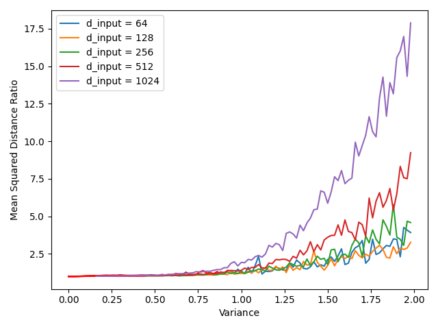
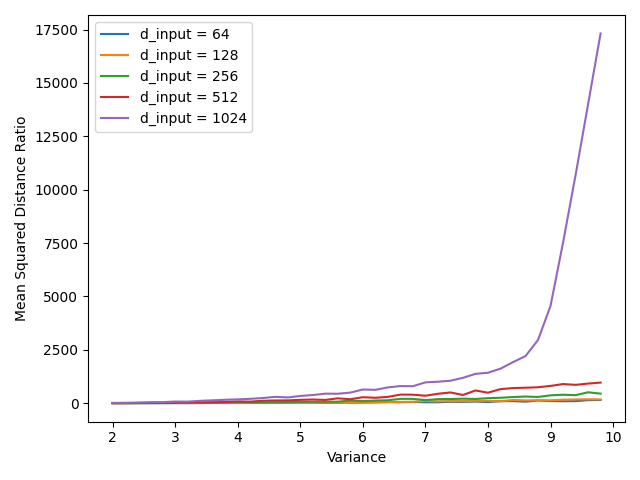
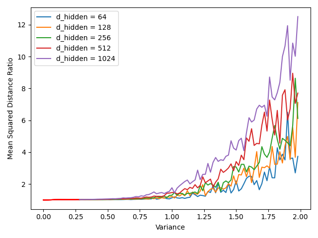
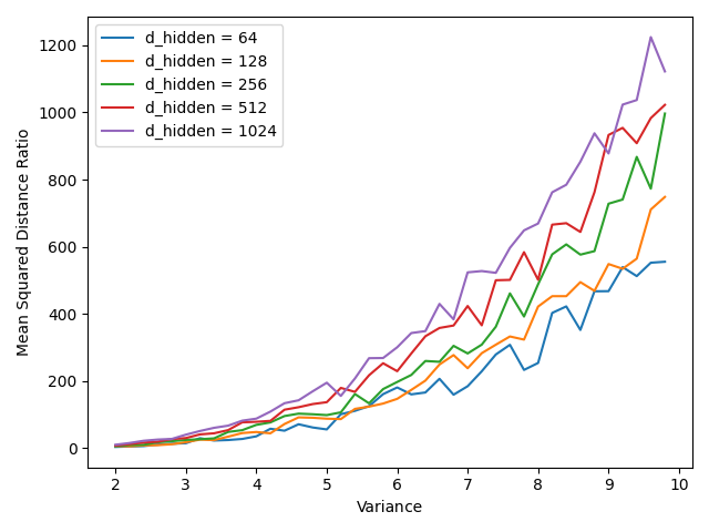
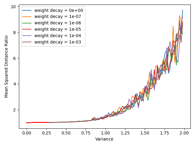
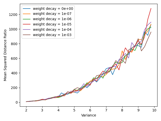
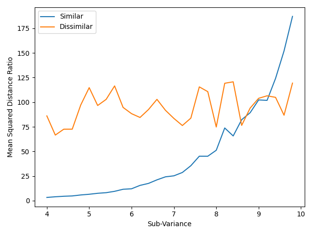
To verify our theoretical analysis and gain more understanding of the fine-grained structure of last-layer representation we provide some synthetic experiment results under the setting of classifying mixture of Gaussian using a 2-layer MLP in Appendix B, which is analogous (although not exactly the same) to the setting analyzed in our theory. Notice that this synthetic experiment is not only helpful to verify the theory, but also able to let us perform controlled experiments by varying different characteristics of the data distribution, architecture, and algorithmic components, to let us better understand how those hyper-parameters play a role in the final-layer representation, and serve as a starting point for a more thorough understanding of the last-layer representation behavior of neural networks.

8 Discussion

In this paper, we initiated the study of the role of the intrinsic structure of the input data distribution on the last-layer representations of neural networks, and in particular, how to reconcile it with the Neural Collapse phenomenon, which is only driven by the explicit labels provided in the training procedure. Through a series of experiments, we provide concrete evidence that the representations can exhibit clear fine-grained structure despite their apparent collapse. While Neural Collapse is an intriguing phenomenon and deserves further studies to understand its cause and consequences, our work calls for more scientific investigations of the structure of neural representations that go beyond Neural Collapse.

We note that the fine-grained representation structure we observed depends on the inductive biases of the network architecture and the training algorithm, and may not appear universally. In our experiments on Coarse CIFAR-10, we observe the fine-grained structure for ResNet and DenseNet, but not for VGG (see Appendices H and G for extended results). We also note that certain choices of learning rate and weight-decay rate lead to stronger fine-grained structure than others. We leave a thorough investigation of such subtlety for future work.

Acknowledgements

WH would like to thank Ruoqi Shen for helpful discussions and contributions in the early stage of this project. JS acknowledges support from NSF DMS-2031899.

References

  • Allen-Zhu & Li (2020) Allen-Zhu, Z. and Li, Y. Towards understanding ensemble, knowledge distillation and self-distillation in deep learning. arXiv preprint arXiv:2012.09816, 2020.
  • Chung & Lu (2006) Chung, F. and Lu, L. Concentration inequalities and martingale inequalities: a survey. Internet mathematics, 3(1):79–127, 2006.
  • Ergen & Pilanci (2021) Ergen, T. and Pilanci, M. Revealing the structure of deep neural networks via convex duality. In International Conference on Machine Learning, pp. 3004–3014. PMLR, 2021.
  • Fang et al. (2021) Fang, C., He, H., Long, Q., and Su, W. J. Exploring deep neural networks via layer-peeled model: Minority collapse in imbalanced training. Proceedings of the National Academy of Sciences, 118(43):e2103091118, 2021.
  • Galanti et al. (2021) Galanti, T., György, A., and Hutter, M. On the role of neural collapse in transfer learning. arXiv preprint arXiv:2112.15121, 2021.
  • Han et al. (2021) Han, X., Papyan, V., and Donoho, D. L. Neural collapse under mse loss: Proximity to and dynamics on the central path. arXiv preprint arXiv:2106.02073, 2021.
  • Hui et al. (2022) Hui, L., Belkin, M., and Nakkiran, P. Limitations of neural collapse for understanding generalization in deep learning. arXiv preprint arXiv:2202.08384, 2022.
  • Ji et al. (2021) Ji, W., Lu, Y., Zhang, Y., Deng, Z., and Su, W. J. An unconstrained layer-peeled perspective on neural collapse. arXiv preprint arXiv:2110.02796, 2021.
  • Levy & Goldberg (2014) Levy, O. and Goldberg, Y. Linguistic regularities in sparse and explicit word representations. In Proceedings of the Eighteenth Conference on Computational Natural Language Learning, pp.  171–180, Ann Arbor, Michigan, June 2014. Association for Computational Linguistics. doi: 10.3115/v1/W14-1618. URL https://aclanthology.org/W14-1618.
  • Lu & Steinerberger (2020) Lu, J. and Steinerberger, S. Neural collapse with cross-entropy loss. arXiv preprint arXiv:2012.08465, 2020.
  • (11) McKenna, R. Tail bounds on the sum of half normal random variables. http://www.ryanhmckenna.com/2021/12/tail-bounds-on-sum-of-half-normal.html.
  • Mixon et al. (2022) Mixon, D. G., Parshall, H., and Pi, J. Neural collapse with unconstrained features. Sampling Theory, Signal Processing, and Data Analysis, 20(2):1–13, 2022.
  • Olah et al. (2017) Olah, C., Mordvintsev, A., and Schubert, L. Feature visualization. Distill, 2017. doi: 10.23915/distill.00007. https://distill.pub/2017/feature-visualization.
  • Papyan et al. (2020) Papyan, V., Han, X., and Donoho, D. L. Prevalence of neural collapse during the terminal phase of deep learning training. Proceedings of the National Academy of Sciences, 117(40):24652–24663, 2020.
  • Rumelhart et al. (1985) Rumelhart, D. E., Hinton, G. E., and Williams, R. J. Learning internal representations by error propagation. Technical report, California Univ San Diego La Jolla Inst for Cognitive Science, 1985.
  • Shen et al. (2022) Shen, R., Bubeck, S., and Gunasekar, S. Data augmentation as feature manipulation. In International Conference on Machine Learning, pp. 19773–19808. PMLR, 2022.
  • Sohoni et al. (2020) Sohoni, N., Dunnmon, J., Angus, G., Gu, A., and Ré, C. No subclass left behind: Fine-grained robustness in coarse-grained classification problems. Advances in Neural Information Processing Systems, 33:19339–19352, 2020.
  • Tirer & Bruna (2022) Tirer, T. and Bruna, J. Extended unconstrained features model for exploring deep neural collapse. arXiv preprint arXiv:2202.08087, 2022.
  • Van der Maaten & Hinton (2008) Van der Maaten, L. and Hinton, G. Visualizing data using t-sne. Journal of machine learning research, 9(11), 2008.
  • van Rooyen et al. (2015) van Rooyen, B., Menon, A. K., and Williamson, R. C. Learning with symmetric label noise: The importance of being unhinged. In Cortes, C., Lawrence, N. D., Lee, D. D., Sugiyama, M., and Garnett, R. (eds.), Advances in Neural Information Processing Systems 28: Annual Conference on Neural Information Processing Systems 2015, December 7-12, 2015, Montreal, Quebec, Canada, pp.  10–18, 2015.
  • Weinan & Wojtowytsch (2022) Weinan, E. and Wojtowytsch, S. On the emergence of simplex symmetry in the final and penultimate layers of neural network classifiers. In Mathematical and Scientific Machine Learning, pp. 270–290. PMLR, 2022.
  • Wojtowytsch et al. (2020) Wojtowytsch, S. et al. On the emergence of simplex symmetry in the final and penultimate layers of neural network classifiers. arXiv preprint arXiv:2012.05420, 2020.
  • Yaras et al. (2022) Yaras, C., Wang, P., Zhu, Z., Balzano, L., and Qu, Q. Neural collapse with normalized features: A geometric analysis over the riemannian manifold. arXiv preprint arXiv:2209.09211, 2022.
  • Zhou et al. (2022) Zhou, J., Li, X., Ding, T., You, C., Qu, Q., and Zhu, Z. On the optimization landscape of neural collapse under mse loss: Global optimality with unconstrained features. arXiv preprint arXiv:2203.01238, 2022.
  • Zhu et al. (2021) Zhu, Z., Ding, T., Zhou, J., Li, X., You, C., Sulam, J., and Qu, Q. A geometric analysis of neural collapse with unconstrained features. Advances in Neural Information Processing Systems, 34:29820–29834, 2021.
  • Zou et al. (2021) Zou, D., Cao, Y., Li, Y., and Gu, Q. Understanding the generalization of adam in learning neural networks with proper regularization. arXiv preprint arXiv:2108.11371, 2021.

Appendix A Proof of Theorem 7.1

Recall that we use unhinged loss (f(𝒙),y)=yf(𝒙)2𝑓𝒙𝑦𝑦𝑓𝒙2\ell(f({\boldsymbol{x}}),y)=-\frac{yf({\boldsymbol{x}})}{2} whose gradient is

(f(𝒙),y)f(𝒙)=y2,𝑓𝒙𝑦𝑓𝒙𝑦2\frac{\partial\ell\left(f({\boldsymbol{x}}),y\right)}{\partial f({\boldsymbol{x}})}=\frac{-y}{2}, (8)

and our goal is to prove

h(𝒙i1)h(𝒙i2)h(𝒙i1)h(𝒙i3).much-less-thannormsubscript𝒙subscript𝑖1subscript𝒙subscript𝑖2normsubscript𝒙subscript𝑖1subscript𝒙subscript𝑖3\left\|h({\boldsymbol{x}}_{i_{1}})-h({\boldsymbol{x}}_{i_{2}})\right\|\ll\|h({\boldsymbol{x}}_{i_{1}})-h({\boldsymbol{x}}_{i_{3}})\|. (9)

A.1 Concentration Lemmas Used

We first introduce some concentration lemmas that we will use.

Lemma A.1 (McKenna ).

Suppose {ψk}k=1nsuperscriptsubscriptsubscript𝜓𝑘𝑘1𝑛\{\psi_{k}\}_{k=1}^{n} are a set of independent Gaussian variables such that ψk𝒩(0,σk2)similar-tosubscript𝜓𝑘𝒩0superscriptsubscript𝜎𝑘2\psi_{k}\sim\mathcal{N}(0,\sigma_{k}^{2}). Then for any t>0𝑡0t>0,

{k=1n|ψk|t}exp(t22k=1nσk2+nlog2).superscriptsubscript𝑘1𝑛subscript𝜓𝑘𝑡superscript𝑡22superscriptsubscript𝑘1𝑛superscriptsubscript𝜎𝑘2𝑛2\displaystyle\mathbb{P}\left\{\sum_{k=1}^{n}|\psi_{k}|\geq t\right\}\leq\exp\left(-\frac{t^{2}}{2\sum_{k=1}^{n}\sigma_{k}^{2}}+n\log 2\right). (10)

In other words, with probability at least exp(n)𝑛\exp(-n), the following inequality holds:

k=1n|ψk|3ni=1nσk2.superscriptsubscript𝑘1𝑛subscript𝜓𝑘3𝑛superscriptsubscript𝑖1𝑛superscriptsubscript𝜎𝑘2\mathbb{\sum}_{k=1}^{n}|\psi_{k}|\geq 3\sqrt{n\sum_{i=1}^{n}\sigma_{k}^{2}}. (11)
Lemma A.2 (Lemma 4 in Shen et al. (2022)).

If 𝐳1𝒩(0,σ12𝐈)similar-tosubscript𝐳1𝒩0superscriptsubscript𝜎12𝐈{\boldsymbol{z}}_{1}\sim\mathcal{N}(0,\sigma_{1}^{2}{\boldsymbol{I}}) and 𝐳2𝒩(0,σ22𝐈)similar-tosubscript𝐳2𝒩0superscriptsubscript𝜎22𝐈{\boldsymbol{z}}_{2}\sim\mathcal{N}\left(0,\sigma_{2}^{2}{\boldsymbol{I}}\right) are d𝑑d-dimensional independent Gaussian vectors, then , we have

{|𝒛1𝒛2|4σ1σ2dlog(2/δ)}δsuperscriptsubscript𝒛1topsubscript𝒛24subscript𝜎1subscript𝜎2𝑑2𝛿𝛿\mathbb{P}\left\{\left|{\boldsymbol{z}}_{1}^{\top}{\boldsymbol{z}}_{2}\right|\geq 4\sigma_{1}\sigma_{2}\sqrt{d\log(2/\delta)}\right\}\leq\delta (12)
Lemma A.3 (Corollary 3 in Shen et al. (2022)).

If 𝐳𝒩(0,σ2𝐈)similar-to𝐳𝒩0superscript𝜎2𝐈{\boldsymbol{z}}\sim\mathcal{N}(0,\sigma^{2}{\boldsymbol{I}}) is a d𝑑d-dimensional Gaussian vector, then for large enough d𝑑d, and δ>2ed/64𝛿2superscript𝑒𝑑64\delta>2e^{-d/64} we have

12σ2d𝒛22σ2d12superscript𝜎2𝑑superscriptnorm𝒛22superscript𝜎2𝑑\frac{1}{2}\sigma^{2}d\leq\|{\boldsymbol{z}}\|^{2}\leq 2\sigma^{2}d (13)
Lemma A.4 (Union Bound).

If there are n𝑛n variables {zk}k=1nsuperscriptsubscriptsubscript𝑧𝑘𝑘1𝑛\{z_{k}\}_{k=1}^{n} (not necessarily independent), and each zksubscript𝑧𝑘z_{k} satisfies

{zkϵk(δ)}δ,subscript𝑧𝑘subscriptitalic-ϵ𝑘𝛿𝛿\mathbb{P}\left\{z_{k}\geq\epsilon_{k}(\delta)\right\}\leq\delta, (14)

then

{k=1nzkk=1nϵk(δ/n)}δsuperscriptsubscript𝑘1𝑛subscript𝑧𝑘superscriptsubscript𝑘1𝑛subscriptitalic-ϵ𝑘𝛿𝑛𝛿\mathbb{P}\left\{\sum_{k=1}^{n}z_{k}\geq\sum_{k=1}^{n}\epsilon_{k}\left(\delta/n\right)\right\}\leq\delta (15)
Proof.

We have that

{k=1nzkk=1nϵk(δ/n)}superscriptsubscript𝑘1𝑛subscript𝑧𝑘superscriptsubscript𝑘1𝑛subscriptitalic-ϵ𝑘𝛿𝑛\displaystyle\mathbb{P}\left\{\sum_{k=1}^{n}z_{k}\leq\sum_{k=1}^{n}\epsilon_{k}\left(\delta/n\right)\right\} k=1n{zkϵk(δ/n)}absentsuperscriptsubscript𝑘1𝑛subscript𝑧𝑘subscriptitalic-ϵ𝑘𝛿𝑛\displaystyle\geq\mathbb{P}\bigcap_{k=1}^{n}\left\{z_{k}\leq\epsilon_{k}(\delta/n)\right\} (16)
k=1n{zkϵk(δ/n)}n+1absentsuperscriptsubscript𝑘1𝑛subscript𝑧𝑘subscriptitalic-ϵ𝑘𝛿𝑛𝑛1\displaystyle\geq\sum_{k=1}^{n}\mathbb{P}\left\{z_{k}\leq\epsilon_{k}(\delta/n)\right\}-n+1 (17)
nn×δnn+1absent𝑛𝑛𝛿𝑛𝑛1\displaystyle\geq n-n\times\frac{\delta}{n}-n+1 (18)
=1δ.absent1𝛿\displaystyle=1-\delta. (19)

Lemma A.5 (Lemma 5 in Shen et al. (2022)).

If there are i.i.d samples {zi}i=1Nsuperscriptsubscriptsubscript𝑧𝑖𝑖1𝑁\{z_{i}\}_{i=1}^{N}, where zi𝒩(0,σ2)similar-tosubscript𝑧𝑖𝒩0superscript𝜎2z_{i}\sim\mathcal{N}(0,\sigma^{2}), then with probability at least 1δ1𝛿1-\delta we have

maxi=1N|zi|σ2log2Nδ.superscriptsubscript𝑖1𝑁subscript𝑧𝑖𝜎22𝑁𝛿\displaystyle\max_{i=1}^{N}|z_{i}|\leq\sigma\sqrt{2\log\frac{2N}{\delta}}. (20)
Lemma A.6 (Anti-Concentration).

If a random variable z𝒩(0,σ2)similar-to𝑧𝒩0superscript𝜎2z\sim\mathcal{N}(0,\sigma^{2}), then for any δ>0𝛿0\delta>0,

{δ<z<δ}<δσ,𝛿𝑧𝛿𝛿𝜎\mathbb{P}\left\{-\delta<z<\delta\right\}<\frac{\delta}{\sigma}, (21)

in other words, with probability higher than 1δ1𝛿1-\delta, we have |z|σδ𝑧𝜎𝛿|z|\geq\sigma\delta.

Proof.
{δ<z<δ}𝛿𝑧𝛿\displaystyle\mathbb{P}\left\{-\delta<z<\delta\right\} =δδ1σ2πexp(x22σ2)dxabsentsuperscriptsubscript𝛿𝛿1𝜎2𝜋superscript𝑥22superscript𝜎2differential-d𝑥\displaystyle=\int_{-\delta}^{\delta}\frac{1}{\sigma\sqrt{2\pi}}\exp\left(-\frac{x^{2}}{2\sigma^{2}}\right)\mathrm{d}x (22)
δδ1σ2πdxabsentsuperscriptsubscript𝛿𝛿1𝜎2𝜋differential-d𝑥\displaystyle\leq\int_{-\delta}^{\delta}\frac{1}{\sigma\sqrt{2\pi}}\mathrm{d}x (23)
=σδ22πabsent𝜎𝛿22𝜋\displaystyle=\sigma\delta\frac{2}{\sqrt{2\pi}} (24)
<σδ.absent𝜎𝛿\displaystyle<\sigma\delta. (25)

A.2 The Dynamics of Model Parameter

In this section, we consider the dynamics of the projection of the model parameters on the “cluster mean” direction and the “noise” direction. Specifically, let 𝝁k=𝝁(p)subscript𝝁𝑘superscript𝝁𝑝{\boldsymbol{\mu}}_{k}={\boldsymbol{\mu}}^{(p)} for k𝒞p𝑘subscript𝒞𝑝k\in{\mathscr{C}}_{p}, we will investigate these two quantities: ζk(t)=𝒘r(t)𝝁ksubscript𝜁𝑘𝑡subscript𝒘𝑟superscript𝑡topsubscript𝝁𝑘\zeta_{k}(t)={\boldsymbol{w}}_{r}(t)^{\top}{\boldsymbol{\mu}}_{k} and ϕk(t)=𝒘r(t)𝝃isubscriptitalic-ϕ𝑘𝑡subscript𝒘𝑟superscript𝑡topsubscript𝝃𝑖\phi_{k}(t)={\boldsymbol{w}}_{r}(t)^{\top}{\boldsymbol{\xi}}_{i}. Notice that ζksubscript𝜁𝑘\zeta_{k} is only dependent on the cluster mean of the cluster which 𝒙ksubscript𝒙𝑘{\boldsymbol{x}}_{k} belongs, so if k𝒞s𝑘subscript𝒞𝑠k\in\mathscr{C}_{s}, we denote ζksubscript𝜁𝑘\zeta_{k} by ζ(s)superscript𝜁𝑠\zeta^{(s)}. Notice that ζksubscript𝜁𝑘\zeta_{k} and ϕksubscriptitalic-ϕ𝑘\phi_{k} are actually depend on neuron index r𝑟r. Throughout this section we fix a neuron index r𝑟r to perform the analysis.

Notice that since we have assumed f(𝒙)𝑓𝒙f({\boldsymbol{x}}) is initialized very small, the activation function σ𝜎\sigma will fall in the interval [1,1]11[-1,1], and hence be a cubic function. Hereinafter unless explicitly mentioned, we will simply use σ(z)=13z3𝜎𝑧13superscript𝑧3\sigma(z)=\frac{1}{3}z^{3} and therefore σ(x)=x2superscript𝜎𝑥superscript𝑥2\sigma^{\prime}(x)=x^{2}. This simplification will be rigorously justified in Theorem 7.1.

For gradient descent with step size η𝜂\eta, the update of 𝒘r(t)subscript𝒘𝑟𝑡{\boldsymbol{w}}_{r}(t) in each step is Δ𝒘(t)=ηL(W)𝒘r(t)Δ𝒘𝑡𝜂𝐿𝑊subscript𝒘𝑟𝑡\Delta{\boldsymbol{w}}(t)=-\eta\frac{\partial L({{W}})}{\partial{\boldsymbol{w}}_{r}(t)}. For other quantities (i.e. ζ,ϕ𝜁italic-ϕ\zeta,\phi), we will use ΔΔ\Delta to denote the update. For example Δζ(s)(t)=Δ𝒘r(t)𝝁(s)Δsuperscript𝜁𝑠𝑡Δsubscript𝒘𝑟superscript𝑡topsuperscript𝝁𝑠\Delta\zeta^{(s)}(t)=\Delta{\boldsymbol{w}}_{r}(t)^{\top}{\boldsymbol{\mu}}^{(s)}.

The gradient of target function w.r.t. 𝒘r(t)subscript𝒘𝑟𝑡{\boldsymbol{w}}_{r}(t) is:

1ηΔ𝒘r(t)1𝜂Δsubscript𝒘𝑟𝑡\displaystyle\frac{1}{\eta}\Delta{\boldsymbol{w}}_{r}(t) =L(W)𝑾r(t)absent𝐿𝑊subscript𝑾𝑟𝑡\displaystyle=-\frac{\partial L(W)}{\partial{\boldsymbol{{\boldsymbol{W}}}}_{r}(t)} (26)
=1ni=1n(f(𝒙i;𝒘r(t)),yi)f(𝒙i,𝒘r(t))𝒘r(t)absent1𝑛superscriptsubscript𝑖1𝑛superscript𝑓subscript𝒙𝑖subscript𝒘𝑟𝑡subscript𝑦𝑖𝑓subscript𝒙𝑖subscript𝒘𝑟𝑡subscript𝒘𝑟𝑡\displaystyle=-\frac{1}{n}\sum_{i=1}^{n}\ell^{\prime}(f({\boldsymbol{x}}_{i};{\boldsymbol{w}}_{r}(t)),y_{i})\frac{\partial f({\boldsymbol{x}}_{i},{\boldsymbol{w}}_{r}(t))}{\partial{\boldsymbol{w}}_{r}(t)} (27)
=1ni=1n(f(𝒙i;𝒘r(t)),yi)σ(𝒙i𝒘r(t))𝒙iabsent1𝑛superscriptsubscript𝑖1𝑛superscript𝑓subscript𝒙𝑖subscript𝒘𝑟𝑡subscript𝑦𝑖superscript𝜎superscriptsubscript𝒙𝑖topsubscript𝒘𝑟𝑡subscript𝒙𝑖\displaystyle=-\frac{1}{n}\sum_{i=1}^{n}\ell^{\prime}(f({\boldsymbol{x}}_{i};{\boldsymbol{w}}_{r}(t)),y_{i})\sigma^{\prime}({\boldsymbol{x}}_{i}^{\top}{\boldsymbol{w}}_{r}(t)){\boldsymbol{x}}_{i} (28)
=12ni=1nyiσ(𝒙i𝒘r(t))𝒙iabsent12𝑛superscriptsubscript𝑖1𝑛subscript𝑦𝑖superscript𝜎superscriptsubscript𝒙𝑖topsubscript𝒘𝑟𝑡subscript𝒙𝑖\displaystyle=\frac{1}{2n}\sum_{i=1}^{n}y_{i}\sigma^{\prime}({\boldsymbol{x}}_{i}^{\top}{\boldsymbol{w}}_{r}(t)){\boldsymbol{x}}_{i} (29)
=12ni=1nyiσ(𝝁i𝒘r(t)+𝝃i𝒘r(t))(𝝁i+𝝃i)absent12𝑛superscriptsubscript𝑖1𝑛subscript𝑦𝑖superscript𝜎superscriptsubscript𝝁𝑖topsubscript𝒘𝑟𝑡superscriptsubscript𝝃𝑖topsubscript𝒘𝑟𝑡subscript𝝁𝑖subscript𝝃𝑖\displaystyle=\frac{1}{2n}\sum_{i=1}^{n}y_{i}\sigma^{\prime}\left({\boldsymbol{\mu}}_{i}^{\top}{\boldsymbol{w}}_{r}(t)+{\boldsymbol{\xi}}_{i}^{\top}{\boldsymbol{w}}_{r}(t)\right)({\boldsymbol{\mu}}_{i}+{\boldsymbol{\xi}}_{i}) (30)
=12np=14𝒙i𝒞pyiσ(𝒘r(t)𝝁(p)+𝒘r(t)𝝃i)(𝝁(p)+𝝃i).absent12𝑛superscriptsubscript𝑝14subscriptsubscript𝒙𝑖subscript𝒞𝑝subscript𝑦𝑖superscript𝜎subscript𝒘𝑟superscript𝑡topsuperscript𝝁𝑝subscript𝒘𝑟superscript𝑡topsubscript𝝃𝑖superscript𝝁𝑝subscript𝝃𝑖\displaystyle=\frac{1}{2n}\sum_{p=1}^{4}\sum_{{\boldsymbol{x}}_{i}\in{\mathscr{C}}_{p}}y_{i}\sigma^{\prime}\left({\boldsymbol{w}}_{r}(t)^{\top}{\boldsymbol{\mu}}^{(p)}+{\boldsymbol{w}}_{r}(t)^{\top}{\boldsymbol{\xi}}_{i}\right)({\boldsymbol{\mu}}^{(p)}+{\boldsymbol{\xi}}_{i}). (31)

Next, we consider the projection of 𝒘r(t)subscript𝒘𝑟𝑡{\boldsymbol{w}}_{r}(t) onto the directions of 𝝁(s)superscript𝝁𝑠{\boldsymbol{\mu}}^{(s)} and 𝝃ksubscript𝝃𝑘{\boldsymbol{\xi}}_{k} separately.

Lemma A.7.

For s{1,2}𝑠12s\in\{1,2\}, we have the following inequality holds with probability at least 1exp(n)1𝑛1-\exp(-n):

|1ηΔζ(s)(t)τ22n𝒙i𝒞sσ[ζ(s)(t)+ϕi(t)]|32τκ.1𝜂Δsuperscript𝜁𝑠𝑡superscript𝜏22𝑛subscriptsubscript𝒙𝑖subscript𝒞𝑠superscript𝜎delimited-[]superscript𝜁𝑠𝑡subscriptitalic-ϕ𝑖𝑡32𝜏𝜅\left|\frac{1}{\eta}\Delta\zeta^{(s)}(t)-\frac{\tau^{2}}{2n}\sum_{{\boldsymbol{x}}_{i}\in{\mathscr{C}}_{s}}\sigma^{\prime}\left[\zeta^{(s)}(t)+\phi_{i}(t)\right]\right|\leq\frac{3}{2}\mathcal{L}\tau\kappa. (32)
Proof.

Notice that since s{1,2}𝑠12s\in\{1,2\}, we have yi=1subscript𝑦𝑖1y_{i}=1 for i𝒞s𝑖subscript𝒞𝑠i\in{\mathscr{C}}_{s}. We have that

2n×1ηΔ𝒘r(t)𝝁(s)=2𝑛1𝜂Δsubscript𝒘𝑟superscript𝑡topsuperscript𝝁𝑠absent\displaystyle 2n\times\frac{1}{\eta}\Delta{\boldsymbol{w}}_{r}(t)^{\top}{\boldsymbol{\mu}}^{(s)}= p=14𝒙i𝒞pyiσ(𝒘r(t)𝝁(p)+𝒘r(t)𝝃i)(𝝁(p)𝝁(s)+𝝃i𝝁(s))superscriptsubscript𝑝14subscriptsubscript𝒙𝑖subscript𝒞𝑝subscript𝑦𝑖superscript𝜎subscript𝒘𝑟superscript𝑡topsuperscript𝝁𝑝subscript𝒘𝑟superscript𝑡topsubscript𝝃𝑖superscript𝝁limit-from𝑝topsuperscript𝝁𝑠superscriptsubscript𝝃𝑖topsuperscript𝝁𝑠\displaystyle\sum_{p=1}^{4}\sum_{{\boldsymbol{x}}_{i}\in{\mathscr{C}}_{p}}y_{i}\sigma^{\prime}\left({\boldsymbol{w}}_{r}(t)^{\top}{\boldsymbol{\mu}}^{(p)}+{\boldsymbol{w}}_{r}(t)^{\top}{\boldsymbol{\xi}}_{i}\right)\left({\boldsymbol{\mu}}^{(p)\top}{\boldsymbol{\mu}}^{(s)}+{\boldsymbol{\xi}}_{i}^{\top}{\boldsymbol{\mu}}^{(s)}\right) (33)
=\displaystyle= 𝒙i𝒞sσ(𝒘r(t)𝝁(s)+𝝃i𝒘r(t))τ2+i=1nyiσ(𝒘r(t)𝝁(s)+𝒘r(t)𝝃i)𝝃i𝝁(s)subscriptsubscript𝒙𝑖subscript𝒞𝑠superscript𝜎subscript𝒘𝑟superscript𝑡topsuperscript𝝁𝑠superscriptsubscript𝝃𝑖topsubscript𝒘𝑟𝑡superscript𝜏2superscriptsubscript𝑖1𝑛subscript𝑦𝑖superscript𝜎subscript𝒘𝑟superscript𝑡topsuperscript𝝁𝑠subscript𝒘𝑟superscript𝑡topsubscript𝝃𝑖superscriptsubscript𝝃𝑖topsuperscript𝝁𝑠\displaystyle\sum_{{\boldsymbol{x}}_{i}\in{\mathscr{C}}_{s}}\sigma^{\prime}\left({\boldsymbol{w}}_{r}(t)^{\top}{\boldsymbol{\mu}}^{(s)}+{\boldsymbol{\xi}}_{i}^{\top}{\boldsymbol{w}}_{r}(t)\right)\tau^{2}+\sum_{i=1}^{n}y_{i}\sigma^{\prime}\left({\boldsymbol{w}}_{r}(t)^{\top}{\boldsymbol{\mu}}^{(s)}+{\boldsymbol{w}}_{r}(t)^{\top}{\boldsymbol{\xi}}_{i}\right){\boldsymbol{\xi}}_{i}^{\top}{\boldsymbol{\mu}}^{(s)} (34)
\displaystyle\in 𝒙i𝒞sσ(𝒘r(t)𝝁(s)+𝝃i𝒘r(t))τ2±(i=1n|𝝃i𝝁(s)|)plus-or-minussubscriptsubscript𝒙𝑖subscript𝒞𝑠superscript𝜎subscript𝒘𝑟superscript𝑡topsuperscript𝝁𝑠superscriptsubscript𝝃𝑖topsubscript𝒘𝑟𝑡superscript𝜏2superscriptsubscript𝑖1𝑛superscriptsubscript𝝃𝑖topsuperscript𝝁𝑠\displaystyle\sum_{{\boldsymbol{x}}_{i}\in{\mathscr{C}}_{s}}\sigma^{\prime}\left({\boldsymbol{w}}_{r}(t)^{\top}{\boldsymbol{\mu}}^{(s)}+{\boldsymbol{\xi}}_{i}^{\top}{\boldsymbol{w}}_{r}(t)\right)\tau^{2}\pm\left(\mathcal{L}\sum_{i=1}^{n}\left|{\boldsymbol{\xi}}_{i}^{\top}{\boldsymbol{\mu}}^{(s)}\right|\right) (35)
=\displaystyle= 𝒙i𝒞sσ(𝒘r(t)𝝁(s)+𝝃i𝒘r(t))τ2±β,plus-or-minussubscriptsubscript𝒙𝑖subscript𝒞𝑠superscript𝜎subscript𝒘𝑟superscript𝑡topsuperscript𝝁𝑠superscriptsubscript𝝃𝑖topsubscript𝒘𝑟𝑡superscript𝜏2𝛽\displaystyle\sum_{{\boldsymbol{x}}_{i}\in{\mathscr{C}}_{s}}\sigma^{\prime}\left({\boldsymbol{w}}_{r}(t)^{\top}{\boldsymbol{\mu}}^{(s)}+{\boldsymbol{\xi}}_{i}^{\top}{\boldsymbol{w}}_{r}(t)\right)\tau^{2}\pm\mathcal{L}\beta, (36)

where β=i=1n|𝝃i𝝁(s)|𝛽superscriptsubscript𝑖1𝑛superscriptsubscript𝝃𝑖topsuperscript𝝁𝑠\beta=\sum_{i=1}^{n}|{\boldsymbol{\xi}}_{i}^{\top}{\boldsymbol{\mu}}^{(s)}|. Since 𝝃i𝝁(s)𝒩(0,κ2τ2)similar-tosuperscriptsubscript𝝃𝑖topsuperscript𝝁𝑠𝒩0superscript𝜅2superscript𝜏2{\boldsymbol{\xi}}_{i}^{\top}{\boldsymbol{\mu}}^{(s)}\sim\mathcal{N}(0,\kappa^{2}\tau^{2}), by Lemma A.1, we have that

{β3nκτ}exp(n).𝛽3𝑛𝜅𝜏𝑛\mathbb{P}\left\{\beta\geq 3n\kappa\tau\right\}\leq\exp(-n). (37)

Combining Equations 36 and 37, we have that with probability at least 1exp(n)1𝑛1-\exp(-n),

2n×1ηΔ𝒘r(t)𝝁(s)2𝑛1𝜂Δsubscript𝒘𝑟superscript𝑡topsuperscript𝝁𝑠\displaystyle 2n\times\frac{1}{\eta}\Delta{\boldsymbol{w}}_{r}(t)^{\top}{\boldsymbol{\mu}}^{(s)} τ2𝒙i𝒞sσ(𝒘r(t)𝝁(s)+𝝃i𝒘r(t))±3nτκ,absentplus-or-minussuperscript𝜏2subscriptsubscript𝒙𝑖subscript𝒞𝑠superscript𝜎subscript𝒘𝑟superscript𝑡topsuperscript𝝁𝑠superscriptsubscript𝝃𝑖topsubscript𝒘𝑟𝑡3𝑛𝜏𝜅\displaystyle\in\tau^{2}\sum_{{\boldsymbol{x}}_{i}\in{\mathscr{C}}_{s}}\sigma^{\prime}\left({\boldsymbol{w}}_{r}(t)^{\top}{\boldsymbol{\mu}}^{(s)}+{\boldsymbol{\xi}}_{i}^{\top}{\boldsymbol{w}}_{r}(t)\right)\pm 3n\mathcal{L}\tau\kappa, (38)

which proves the proposition. ∎

Lemma A.8.

For k𝒞1𝒞2𝑘subscript𝒞1subscript𝒞2k\in\mathscr{C}_{1}\cup\mathscr{C}_{2}, if there exists a constant c(n)>0superscript𝑐𝑛0c^{(n)}>0 such that nc(n)κdτ𝑛superscript𝑐𝑛𝜅𝑑𝜏n\leq c^{(n)}\frac{\kappa d}{\tau}, then we have

{κ2d4nσ(ϕk(t)+ζk(t))52κτ1ηΔϕk(t)3κ2d4nσ(ϕk(t)+ζk(t))+52κτ}1δ,superscript𝜅2𝑑4𝑛superscript𝜎subscriptitalic-ϕ𝑘𝑡subscript𝜁𝑘𝑡52𝜅𝜏1𝜂Δsubscriptitalic-ϕ𝑘𝑡3superscript𝜅2𝑑4𝑛superscript𝜎subscriptitalic-ϕ𝑘𝑡subscript𝜁𝑘𝑡52𝜅𝜏1𝛿\mathbb{P}\left\{\frac{\kappa^{2}d}{4n}\sigma^{\prime}(\phi_{k}(t)+\zeta_{k}(t))-\frac{5}{2}\kappa\tau\mathcal{L}\leq\frac{1}{\eta}\Delta\phi_{k}(t)\leq\frac{3\kappa^{2}d}{4n}\sigma^{\prime}(\phi_{k}(t)+\zeta_{k}(t))+\frac{5}{2}\kappa\tau\mathcal{L}\right\}\geq 1-\delta, (39)

where δ=exp(n)+2nexp(1𝔠2)+2exp(d/64)𝛿𝑛2𝑛1superscript𝔠22𝑑64\delta=\exp(-n)+2n\exp\left(-\frac{1}{\mathfrak{c}^{2}}\right)+2\exp(-d/64).

Proof.

For the noise term 𝝃ksubscript𝝃𝑘{\boldsymbol{\xi}}_{k}, notice that since k𝒞1𝒞2𝑘subscript𝒞1subscript𝒞2k\in\mathscr{C}_{1}\cup\mathscr{C}_{2}, we have yk=1subscript𝑦𝑘1y_{k}=1, and

2n×1ηΔ𝒘r(t)𝝃k=2𝑛1𝜂Δsubscript𝒘𝑟superscript𝑡topsubscript𝝃𝑘absent\displaystyle 2n\times\frac{1}{\eta}\Delta{\boldsymbol{w}}_{r}(t)^{\top}{\boldsymbol{\xi}}_{k}= σ[𝝁k𝒘r(t)+𝝃k𝒘r(t)]𝝃k2+σ[𝝁k𝒘r(t)+𝝃k𝒘r(t)]𝝃k𝝁ksuperscript𝜎delimited-[]superscriptsubscript𝝁𝑘topsubscript𝒘𝑟𝑡superscriptsubscript𝝃𝑘topsubscript𝒘𝑟𝑡superscriptnormsubscript𝝃𝑘2superscript𝜎delimited-[]superscriptsubscript𝝁𝑘topsubscript𝒘𝑟𝑡superscriptsubscript𝝃𝑘topsubscript𝒘𝑟𝑡superscriptsubscript𝝃𝑘topsubscript𝝁𝑘\displaystyle\sigma^{\prime}\left[{\boldsymbol{\mu}}_{k}^{\top}{\boldsymbol{w}}_{r}(t)+{\boldsymbol{\xi}}_{k}^{\top}{\boldsymbol{w}}_{r}(t)\right]\|{\boldsymbol{\xi}}_{k}\|^{2}+\sigma^{\prime}\left[{\boldsymbol{\mu}}_{k}^{\top}{\boldsymbol{w}}_{r}(t)+{\boldsymbol{\xi}}_{k}^{\top}{\boldsymbol{w}}_{r}(t)\right]{\boldsymbol{\xi}}_{k}^{\top}{\boldsymbol{\mu}}_{k} (40)
+p=14𝒙i𝒞pikyiσ(𝒘r(t)𝝁(p)+𝒘r(t)𝝃i)(𝝃k𝝁(p)+𝝃k𝝃i)superscriptsubscript𝑝14subscriptFRACOPsubscript𝒙𝑖subscript𝒞𝑝𝑖𝑘subscript𝑦𝑖superscript𝜎subscript𝒘𝑟superscript𝑡topsuperscript𝝁𝑝subscript𝒘𝑟superscript𝑡topsubscript𝝃𝑖superscriptsubscript𝝃𝑘topsuperscript𝝁𝑝superscriptsubscript𝝃𝑘topsubscript𝝃𝑖\displaystyle+\sum_{p=1}^{4}\sum_{{\boldsymbol{x}}_{i}\in{\mathscr{C}}_{p}\atop i\neq k}y_{i}\sigma^{\prime}({\boldsymbol{w}}_{r}(t)^{\top}{\boldsymbol{\mu}}^{(p)}+{\boldsymbol{w}}_{r}(t)^{\top}{\boldsymbol{\xi}}_{i})\left({\boldsymbol{\xi}}_{k}^{\top}{\boldsymbol{\mu}}^{(p)}+{\boldsymbol{\xi}}_{k}^{\top}{\boldsymbol{\xi}}_{i}\right) (41)
\displaystyle\in σ[𝝁k𝒘r(t)+𝝃k𝒘r(t)]𝝃k2±[|𝝃k𝝁k|+p=14𝒙i𝒞pik|𝝃k𝝁(p)+𝝃k𝝃i|]plus-or-minussuperscript𝜎delimited-[]superscriptsubscript𝝁𝑘topsubscript𝒘𝑟𝑡superscriptsubscript𝝃𝑘topsubscript𝒘𝑟𝑡superscriptnormsubscript𝝃𝑘2delimited-[]superscriptsubscript𝝃𝑘topsubscript𝝁𝑘superscriptsubscript𝑝14subscriptFRACOPsubscript𝒙𝑖subscript𝒞𝑝𝑖𝑘superscriptsubscript𝝃𝑘topsuperscript𝝁𝑝superscriptsubscript𝝃𝑘topsubscript𝝃𝑖\displaystyle\sigma^{\prime}\left[{\boldsymbol{\mu}}_{k}^{\top}{\boldsymbol{w}}_{r}(t)+{\boldsymbol{\xi}}_{k}^{\top}{\boldsymbol{w}}_{r}(t)\right]\|{\boldsymbol{\xi}}_{k}\|^{2}\pm\left[\mathcal{L}\left|{\boldsymbol{\xi}}_{k}^{\top}{\boldsymbol{\mu}}_{k}\right|+\sum_{p=1}^{4}\sum_{{\boldsymbol{x}}_{i}\in{\mathscr{C}}_{p}\atop i\neq k}\mathcal{L}\left|{\boldsymbol{\xi}}_{k}^{\top}{\boldsymbol{\mu}}^{(p)}+{\boldsymbol{\xi}}_{k}^{\top}{\boldsymbol{\xi}}_{i}\right|\right] (42)
\displaystyle\subseteq σ[𝝁k𝒘r(t)+𝝃k𝒘r(t)]𝝃k2±[i=1n|𝝃i𝝁i|+1inik|𝝃k𝝃i|]plus-or-minussuperscript𝜎delimited-[]superscriptsubscript𝝁𝑘topsubscript𝒘𝑟𝑡superscriptsubscript𝝃𝑘topsubscript𝒘𝑟𝑡superscriptnormsubscript𝝃𝑘2delimited-[]superscriptsubscript𝑖1𝑛superscriptsubscript𝝃𝑖topsubscript𝝁𝑖subscriptFRACOP1𝑖𝑛𝑖𝑘superscriptsubscript𝝃𝑘topsubscript𝝃𝑖\displaystyle\sigma^{\prime}\left[{\boldsymbol{\mu}}_{k}^{\top}{\boldsymbol{w}}_{r}(t)+{\boldsymbol{\xi}}_{k}^{\top}{\boldsymbol{w}}_{r}(t)\right]\|{\boldsymbol{\xi}}_{k}\|^{2}\pm\left[\sum_{i=1}^{n}\mathcal{L}\left|{\boldsymbol{\xi}}_{i}^{\top}{\boldsymbol{\mu}}_{i}\right|+\sum_{1\leq i\leq n\atop i\neq k}\mathcal{L}\left|{\boldsymbol{\xi}}_{k}^{\top}{\boldsymbol{\xi}}_{i}\right|\right] (43)
=\displaystyle= σ[𝝁k𝒘r(t)+𝝃k𝒘r(t)]𝝃k2±βplus-or-minussuperscript𝜎delimited-[]superscriptsubscript𝝁𝑘topsubscript𝒘𝑟𝑡superscriptsubscript𝝃𝑘topsubscript𝒘𝑟𝑡superscriptnormsubscript𝝃𝑘2𝛽\displaystyle\sigma^{\prime}\left[{\boldsymbol{\mu}}_{k}^{\top}{\boldsymbol{w}}_{r}(t)+{\boldsymbol{\xi}}_{k}^{\top}{\boldsymbol{w}}_{r}(t)\right]\|{\boldsymbol{\xi}}_{k}\|^{2}\pm\mathcal{L}\beta (44)

where

β=i=1n|𝝃k𝝁i|+1inik|𝝃k𝝃i|.𝛽superscriptsubscript𝑖1𝑛superscriptsubscript𝝃𝑘topsubscript𝝁𝑖subscriptFRACOP1𝑖𝑛𝑖𝑘superscriptsubscript𝝃𝑘topsubscript𝝃𝑖\displaystyle\beta=\sum_{i=1}^{n}\left|{\boldsymbol{\xi}}_{k}^{\top}{\boldsymbol{\mu}}_{i}\right|+\sum_{1\leq i\leq n\atop i\neq k}\left|{\boldsymbol{\xi}}_{k}^{\top}{\boldsymbol{\xi}}_{i}\right|. (45)

Notice that nc(n)κdτ𝑛superscript𝑐𝑛𝜅𝑑𝜏n\leq\frac{c^{(n)}\kappa d}{\tau}. Let δ1=exp(n)subscript𝛿1𝑛\delta_{1}=\exp(-n). From Lemma A.1, with probability at least 1δ11subscript𝛿11-\delta_{1}, we have

i=1n|𝝃k𝝁i|3τκn.superscriptsubscript𝑖1𝑛superscriptsubscript𝝃𝑘topsubscript𝝁𝑖3𝜏𝜅𝑛\mathbb{\sum}_{i=1}^{n}\left|{\boldsymbol{\xi}}_{k}^{\top}{\boldsymbol{\mu}}_{i}\right|\leq 3\tau\kappa n. (46)

From Lemma A.2 and Lemma A.1, we have that with probability at least 1δ21subscript𝛿21-\delta_{2}, we have

ik|𝝃k𝝃i|2nκ2dlog(2n/δ2).subscript𝑖𝑘superscriptsubscript𝝃𝑘topsubscript𝝃𝑖2𝑛superscript𝜅2𝑑2𝑛subscript𝛿2\sum_{i\neq k}\left|{\boldsymbol{\xi}}_{k}^{\top}{\boldsymbol{\xi}}_{i}\right|\leq 2n\kappa^{2}\sqrt{d\log(2n/\delta_{2})}. (47)

Take δ2=2nexp(1𝔠2)subscript𝛿22𝑛1superscript𝔠2\delta_{2}=2n\exp\left(-\frac{1}{\mathfrak{c}^{2}}\right), we get

ik|𝝃k𝝃i|subscript𝑖𝑘superscriptsubscript𝝃𝑘topsubscript𝝃𝑖\displaystyle\sum_{i\neq k}\left|{\boldsymbol{\xi}}_{k}^{\top}{\boldsymbol{\xi}}_{i}\right| 2nκ2dlog(2n/δ2).absent2𝑛superscript𝜅2𝑑2𝑛subscript𝛿2\displaystyle\leq 2n\kappa^{2}\sqrt{d\log(2n/\delta_{2})}. (48)
2nκ2d×τ2κ2dabsent2𝑛superscript𝜅2𝑑superscript𝜏2superscript𝜅2𝑑\displaystyle\leq 2n\kappa^{2}\sqrt{d\times\frac{\tau^{2}}{\kappa^{2}d}} (49)
=2nκτabsent2𝑛𝜅𝜏\displaystyle=2n\kappa\tau (50)

To summery, with probability at least 1δ1δ21subscript𝛿1subscript𝛿21-\delta_{1}-\delta_{2}, we have

2nβ52κτ.2𝑛𝛽52𝜅𝜏\frac{\mathcal{L}}{2n}\beta\leq\frac{5}{2}\kappa\tau\mathcal{L}. (51)

.

From Lemma A.3, with δ3>2exp(d/64)subscript𝛿32𝑑64\delta_{3}>2\exp(-d/64), we have

12κ2d𝝃k232κ2d.12superscript𝜅2𝑑superscriptnormsubscript𝝃𝑘232superscript𝜅2𝑑\frac{1}{2}\kappa^{2}d\leq\|{\boldsymbol{\xi}}_{k}\|^{2}\leq\frac{3}{2}\kappa^{2}d. (52)

Combining Equations 51 and 52, the proposition is proved.

To summarize, Lemma A.7 shows that with probability at least 1δ11subscript𝛿11-\delta_{1}, where δ1=exp(n)subscript𝛿1𝑛\delta_{1}=-\exp(-n), we have

ζ(s)(t+1)ζ(s)(t)τ2η2n𝒙i𝒞sσ[ζ(s)(t)+ϕi(t)]±τ2η2×3κτsuperscript𝜁𝑠𝑡1superscript𝜁𝑠𝑡plus-or-minussuperscript𝜏2𝜂2𝑛subscriptsubscript𝒙𝑖subscript𝒞𝑠superscript𝜎delimited-[]superscript𝜁𝑠𝑡subscriptitalic-ϕ𝑖𝑡superscript𝜏2𝜂23𝜅𝜏\zeta^{(s)}(t+1)-\zeta^{(s)}(t)\in\frac{\tau^{2}\eta}{2n}\sum_{{\boldsymbol{x}}_{i}\in{\mathscr{C}}_{s}}\sigma^{\prime}\left[\zeta^{(s)}(t)+\phi_{i}(t)\right]\pm\frac{\tau^{2}\eta}{2}\times\frac{3\mathcal{L}\kappa}{\tau} (53)

and with probability at least 1δ21subscript𝛿21-\delta_{2}, where δ2=exp(n)+2nexp(c2)+2exp(d/64)subscript𝛿2𝑛2𝑛superscript𝑐22𝑑64\delta_{2}=\exp(-n)+2n\exp\left(-c^{-2}\right)+2\exp(-d/64), we have

ϕk(t+1)ϕk(t)subscriptitalic-ϕ𝑘𝑡1subscriptitalic-ϕ𝑘𝑡\displaystyle\phi_{k}(t+1)-\phi_{k}(t) =ηddtϕk(t)absent𝜂dd𝑡subscriptitalic-ϕ𝑘𝑡\displaystyle=\eta\frac{\mathrm{d}}{\mathrm{d}t}\phi_{k}(t) (54)
η[κ2d4nσ(ϕk(t)+ζk(t))52κτ,3κ2d4nσ(ϕk(t)+ζk(t))+5c(n)κ2dn]absent𝜂superscript𝜅2𝑑4𝑛superscript𝜎subscriptitalic-ϕ𝑘𝑡subscript𝜁𝑘𝑡52𝜅𝜏3superscript𝜅2𝑑4𝑛superscript𝜎subscriptitalic-ϕ𝑘𝑡subscript𝜁𝑘𝑡5superscript𝑐𝑛superscript𝜅2𝑑𝑛\displaystyle\in\eta\left[\frac{\kappa^{2}d}{4n}\sigma^{\prime}(\phi_{k}(t)+\zeta_{k}(t))-\frac{5}{2}\kappa\tau\mathcal{L},\frac{3\kappa^{2}d}{4n}\sigma^{\prime}(\phi_{k}(t)+\zeta_{k}(t))+\frac{5c^{(n)}\kappa^{2}d\mathcal{L}}{n}\right] (55)
η[κ2d4nσ(|ϕk(t)|+|ζk(t)|)5c(n)κ2dn,3κ2d4nσ(|ϕk(t)|+|ζk(t)|)+52κτ].absent𝜂superscript𝜅2𝑑4𝑛superscript𝜎subscriptitalic-ϕ𝑘𝑡subscript𝜁𝑘𝑡5superscript𝑐𝑛superscript𝜅2𝑑𝑛3superscript𝜅2𝑑4𝑛superscript𝜎subscriptitalic-ϕ𝑘𝑡subscript𝜁𝑘𝑡52𝜅𝜏\displaystyle\subseteq\eta\left[\frac{\kappa^{2}d}{4n}\sigma^{\prime}(|\phi_{k}(t)|+|\zeta_{k}(t)|)-\frac{5c^{(n)}\kappa^{2}d\mathcal{L}}{n},\frac{3\kappa^{2}d}{4n}\sigma^{\prime}(|\phi_{k}(t)|+|\zeta_{k}(t)|)+\frac{5}{2}\kappa\tau\mathcal{L}\right]. (56)
Lemma A.9.

Let s{1,2}𝑠12s\in\{1,2\}. Suppose ζ(s)superscript𝜁𝑠\zeta^{(s)} is initialized by ζ(s)(0)superscript𝜁𝑠0\zeta^{(s)}(0), and there exists constants c(t)(0,81+8𝔠)superscript𝑐𝑡0818𝔠c^{(t)}\in\left(0,\frac{8}{1+8\mathfrak{c}}\right) and C(ϕ)>0superscript𝐶italic-ϕ0C^{(\phi)}>0 such that the following conditions hold for t0<c(t)(τ2η|ζ(s)(0)|)1subscript𝑡0superscript𝑐𝑡superscriptsuperscript𝜏2𝜂superscript𝜁𝑠01t_{0}<c^{(t)}\left(\tau^{2}\eta\left|\zeta^{(s)}(0)\right|\right)^{-1}:

  1. 1.

    tt0for-all𝑡subscript𝑡0\forall t\leq t_{0}, if ζ(s)(0)>0superscript𝜁𝑠00\zeta^{(s)}(0)>0, we have [ζ(s)(0)1(18𝔠)ητ2t]1ζ(s)(t)[ζ(s)(0)1(18+𝔠)ητ2t]1superscriptdelimited-[]superscript𝜁𝑠superscript0118𝔠𝜂superscript𝜏2𝑡1superscript𝜁𝑠𝑡superscriptdelimited-[]superscript𝜁𝑠superscript0118𝔠𝜂superscript𝜏2𝑡1\left[\zeta^{(s)}(0)^{-1}-\left(\frac{1}{8}-\mathfrak{c}\right)\eta\tau^{2}t\right]^{-1}\leq\zeta^{(s)}(t)\leq\left[\zeta^{(s)}(0)^{-1}-\left(\frac{1}{8}+\mathfrak{c}\right)\eta\tau^{2}t\right]^{-1}, while if ζ(s)(0)<0superscript𝜁𝑠00\zeta^{(s)}(0)<0, we have ζ(s)(0)ζ(s)(t)ζ(s)(0)+(18+𝔠)ητ2t|ζ(s)(0)|2superscript𝜁𝑠0superscript𝜁𝑠𝑡superscript𝜁𝑠018𝔠𝜂superscript𝜏2𝑡superscriptsuperscript𝜁𝑠02\zeta^{(s)}(0)\leq\zeta^{(s)}(t)\leq\zeta^{(s)}(0)+\left(\frac{1}{8}+\mathfrak{c}\right)\eta\tau^{2}t|\zeta^{(s)}(0)|^{2},

  2. 2.

    tt0,informulae-sequencefor-all𝑡subscript𝑡0for-all𝑖𝑛\forall t\leq t_{0},\forall i\leq n, |ϕi(t)|C(ϕ)𝔠2n|ζ(s)(t)|+𝔠8|ζ(s)(0)|subscriptitalic-ϕ𝑖𝑡superscript𝐶italic-ϕsuperscript𝔠2𝑛superscript𝜁𝑠𝑡𝔠8superscript𝜁𝑠0|\phi_{i}(t)|\leq\frac{C^{(\phi)}\mathfrak{c}^{2}}{n}\left|\zeta^{(s)}(t)\right|+\frac{\mathfrak{c}}{8}|\zeta^{(s)}(0)|;

  3. 3.

    32n𝔠2d|ζ(s)(0)|𝔠(8c(t))16ητ232𝑛superscript𝔠2𝑑superscript𝜁𝑠0𝔠8superscript𝑐𝑡16𝜂superscript𝜏2\sqrt{\frac{32\mathcal{L}n}{\mathfrak{c}^{2}\sqrt{d}}}\leq|\zeta^{(s)}(0)|\leq\frac{\mathfrak{c}\left(8-{c^{(t)}}\right)}{16\eta\tau^{2}};

  4. 4.

    𝔠min{nC(ϕ)4,(n48)13,18}𝔠𝑛superscript𝐶italic-ϕ4superscript𝑛481318\mathfrak{c}\leq\min\left\{\frac{nC^{(\phi)}}{4},\left(\frac{n}{48}\right)^{\frac{1}{3}},\frac{1}{8}\right\},

and ζ(s)superscript𝜁𝑠\zeta^{(s)} is updated as described in Equation 53, then we have:

  1. a)

    tt0,|ζ(s)(t)|>12|ζ(s)(0)|formulae-sequencefor-all𝑡subscript𝑡0superscript𝜁𝑠𝑡12superscript𝜁𝑠0\forall t\leq t_{0},\left|\zeta^{(s)}(t)\right|>\frac{1}{2}\left|\zeta^{(s)}(0)\right|;

  2. b)

    (18𝔠2)ητ2ζ(s)(t0)2ζ(s)(t0+1)ζ(s)(t0)(18+𝔠2)ητ2ζ(s)(t0)218𝔠2𝜂superscript𝜏2superscript𝜁𝑠superscriptsubscript𝑡02superscript𝜁𝑠subscript𝑡01superscript𝜁𝑠subscript𝑡018𝔠2𝜂superscript𝜏2superscript𝜁𝑠superscriptsubscript𝑡02\left(\frac{1}{8}-\frac{\mathfrak{c}}{2}\right)\eta\tau^{2}\zeta^{(s)}(t_{0})^{2}\leq\zeta^{(s)}(t_{0}+1)-\zeta^{(s)}(t_{0})\leq\left(\frac{1}{8}+\frac{\mathfrak{c}}{2}\right)\eta\tau^{2}\zeta^{(s)}(t_{0})^{2};

  3. c)

    If ζ(s)(0)>0superscript𝜁𝑠00\zeta^{(s)}(0)>0, we have

    [ζ(s)(0)1(18𝔠)ητ2(t0+1)]1ζ(s)(t0+1)[ζ(s)(0)1(18+𝔠)ητ2(t0+1)]1,superscriptdelimited-[]superscript𝜁𝑠superscript0118𝔠𝜂superscript𝜏2subscript𝑡011superscript𝜁𝑠subscript𝑡01superscriptdelimited-[]superscript𝜁𝑠superscript0118𝔠𝜂superscript𝜏2subscript𝑡011\displaystyle\left[\zeta^{(s)}(0)^{-1}-\left(\frac{1}{8}-\mathfrak{c}\right)\eta\tau^{2}(t_{0}+1)\right]^{-1}\leq\zeta^{(s)}(t_{0}+1)\leq\left[\zeta^{(s)}(0)^{-1}-\left(\frac{1}{8}+\mathfrak{c}\right)\eta\tau^{2}(t_{0}+1)\right]^{-1}, (57)

    while if ζ(s)(0)<0superscript𝜁𝑠00\zeta^{(s)}(0)<0 we have ζ(s)(0)ζ(s)(t0+1)ζ(s)(0)+ητ2(t0+1)|ζ(s)(0)|2superscript𝜁𝑠0superscript𝜁𝑠subscript𝑡01superscript𝜁𝑠0𝜂superscript𝜏2subscript𝑡01superscriptsuperscript𝜁𝑠02\zeta^{(s)}(0)\leq\zeta^{(s)}(t_{0}+1)\leq\zeta^{(s)}(0)+\eta\tau^{2}(t_{0}+1)|\zeta^{(s)}(0)|^{2}.

Proof.
  • First, notice that since t<t0<c(t)(ητ2|ζ(s)(0)|)1𝑡subscript𝑡0superscript𝑐𝑡superscript𝜂superscript𝜏2superscript𝜁𝑠01t<t_{0}<c^{(t)}\left(\eta\tau^{2}|\zeta^{(s)}(0)|\right)^{-1}, we have ητ2t|ζ(s)(0)|2c(t)|ζ(s)(0)|𝜂superscript𝜏2𝑡superscriptsuperscript𝜁𝑠02superscript𝑐𝑡superscript𝜁𝑠0\eta\tau^{2}t|\zeta^{(s)}(0)|^{2}\leq c^{(t)}|\zeta^{(s)}(0)|, and

    ζ(s)(t)ζ(s)(0)+(18+𝔠)ητ2t|ζ(s)(0)|2ζ(s)(0)+c(t)(18+𝔠)|ζ(s)(0)|0.superscript𝜁𝑠𝑡superscript𝜁𝑠018𝔠𝜂superscript𝜏2𝑡superscriptsuperscript𝜁𝑠02superscript𝜁𝑠0superscript𝑐𝑡18𝔠superscript𝜁𝑠00\displaystyle\zeta^{(s)}(t)\leq\zeta^{(s)}(0)+\left(\frac{1}{8}+\mathfrak{c}\right)\eta\tau^{2}t|\zeta^{(s)}(0)|^{2}\leq\zeta^{(s)}(0)+c^{(t)}\left(\frac{1}{8}+\mathfrak{c}\right)|\zeta^{(s)}(0)|\leq 0. (58)

    If ζ(s)(0)<0superscript𝜁𝑠00\zeta^{(s)}(0)<0, then

    |ζ(s)(t)||ζ(s)(0)|ητ2t|ζ(s)(0)|2(1c(t))|ζ(s)(0)|12|ζ(s)(0)|.superscript𝜁𝑠𝑡superscript𝜁𝑠0𝜂superscript𝜏2𝑡superscriptsuperscript𝜁𝑠021superscript𝑐𝑡superscript𝜁𝑠012superscript𝜁𝑠0\displaystyle|\zeta^{(s)}(t)|\geq|\zeta^{(s)}(0)|-\eta\tau^{2}t|\zeta^{(s)}(0)|^{2}\geq\left(1-c^{(t)}\right)|\zeta^{(s)}(0)|\geq\frac{1}{2}|\zeta^{(s)}(0)|. (59)

    While if ζ(s)(0)>0superscript𝜁𝑠00\zeta^{(s)}(0)>0, then

    |ζ(s)(t)|[|ζ(s)(0)|1(18𝔠)τ2ηt]1|ζ(s)(0)|.superscript𝜁𝑠𝑡superscriptdelimited-[]superscriptsuperscript𝜁𝑠0118𝔠superscript𝜏2𝜂𝑡1superscript𝜁𝑠0\displaystyle\left|\zeta^{(s)}(t)\right|\geq\left[\left|\zeta^{(s)}(0)\right|^{-1}-\left(\frac{1}{8}-\mathfrak{c}\right)\tau^{2}\eta t\right]^{-1}\geq|\zeta^{(s)}(0)|. (60)

    Equation 59 and Equation 60 together proves Result a).

  • Notice that from Condition 4 we have 𝔠2C(ϕ)n𝔠4superscript𝔠2superscript𝐶italic-ϕ𝑛𝔠4\frac{\mathfrak{c}^{2}C^{(\phi)}}{n}\leq\frac{\mathfrak{c}}{4}. From Condition 2, we have

    ζ(s)(t)+ϕi(t)|ζ(s)(t)||ϕi(t)|(1𝔠4)|ζ(s)(t)|𝔠8|ζ(s)(0)|(1𝔠2)|ζ(s)(t)|superscript𝜁𝑠𝑡subscriptitalic-ϕ𝑖𝑡superscript𝜁𝑠𝑡subscriptitalic-ϕ𝑖𝑡1𝔠4superscript𝜁𝑠𝑡𝔠8superscript𝜁𝑠01𝔠2superscript𝜁𝑠𝑡\displaystyle\zeta^{(s)}(t)+\phi_{i}(t)\geq\left|\zeta^{(s)}(t)\right|-\left|\phi_{i}(t)\right|\geq\left(1-\frac{\mathfrak{c}}{4}\right)\left|\zeta^{(s)}(t)\right|-\frac{\mathfrak{c}}{8}|\zeta^{(s)}(0)|\geq\left(1-\frac{\mathfrak{c}}{2}\right)|\zeta^{(s)}(t)| (61)

    and

    ζ(s)(t)+ϕi(t)|ζ(s)(t)|+|ϕi(t)|(1+𝔠4)|ζ(s)(t)|+𝔠8|ζ(s)(0)|(1+𝔠2)|ζ(s)(t)|.superscript𝜁𝑠𝑡subscriptitalic-ϕ𝑖𝑡superscript𝜁𝑠𝑡subscriptitalic-ϕ𝑖𝑡1𝔠4superscript𝜁𝑠𝑡𝔠8superscript𝜁𝑠01𝔠2superscript𝜁𝑠𝑡\displaystyle\zeta^{(s)}(t)+\phi_{i}(t)\leq\left|\zeta^{(s)}(t)\right|+\left|\phi_{i}(t)\right|\leq\left(1+\frac{\mathfrak{c}}{4}\right)\left|\zeta^{(s)}(t)\right|+\frac{\mathfrak{c}}{8}|\zeta^{(s)}(0)|\leq\left(1+\frac{\mathfrak{c}}{2}\right)|\zeta^{(s)}(t)|. (62)

    Therefore we have

    1n𝒙i𝒞sσ[ζ(s)(t)+ϕi(t)]1𝑛subscriptsubscript𝒙𝑖subscript𝒞𝑠superscript𝜎delimited-[]superscript𝜁𝑠𝑡subscriptitalic-ϕ𝑖𝑡\displaystyle\frac{1}{n}\sum_{{\boldsymbol{x}}_{i}\in{\mathscr{C}}_{s}}\sigma^{\prime}\left[\zeta^{(s)}(t)+\phi_{i}(t)\right] =1n𝒙i𝒞s[ζ(s)(t)+ϕi(t)]2absent1𝑛subscriptsubscript𝒙𝑖subscript𝒞𝑠superscriptdelimited-[]superscript𝜁𝑠𝑡subscriptitalic-ϕ𝑖𝑡2\displaystyle=\frac{1}{n}\sum_{{\boldsymbol{x}}_{i}\in{\mathscr{C}}_{s}}\left[\zeta^{(s)}(t)+\phi_{i}(t)\right]^{2} (63)
    1n𝒙i𝒞s(1±𝔠2)2ζ(s)(t)2absent1𝑛subscriptsubscript𝒙𝑖subscript𝒞𝑠superscriptplus-or-minus1𝔠22superscript𝜁𝑠superscript𝑡2\displaystyle\in\frac{1}{n}\sum_{{\boldsymbol{x}}_{i}\in{\mathscr{C}}_{s}}\left(1\pm\frac{\mathfrak{c}}{2}\right)^{2}\zeta^{(s)}(t)^{2} (64)
    =14(1±𝔠2)2ζ(s)(t)2.absent14superscriptplus-or-minus1𝔠22superscript𝜁𝑠superscript𝑡2\displaystyle=\frac{1}{4}\left(1\pm\frac{\mathfrak{c}}{2}\right)^{2}\zeta^{(s)}(t)^{2}. (65)
    14(1±2𝔠)ζ(s)(t)2.absent14plus-or-minus12𝔠superscript𝜁𝑠superscript𝑡2\displaystyle\subseteq\frac{1}{4}(1\pm 2\mathfrak{c})\zeta^{(s)}(t)^{2}. (66)

    From Condition 3, Condition 4 and Result a), we have

    3κτ𝔠8ζ(s)(0)2𝔠2ζ(s)(t)2.3𝜅𝜏𝔠8superscript𝜁𝑠superscript02𝔠2superscript𝜁𝑠superscript𝑡2\displaystyle\frac{3\mathcal{L}\kappa}{\tau}\leq\frac{\mathfrak{c}}{8}\zeta^{(s)}(0)^{2}\leq\frac{\mathfrak{c}}{2}\zeta^{(s)}(t)^{2}. (67)

    Subtracting Equation 66 and Equation 67 into the update rule Equation 53, we have

    ζ(s)(t+1)ζ(s)(t)superscript𝜁𝑠𝑡1superscript𝜁𝑠𝑡\displaystyle\zeta^{(s)}(t+1)-\zeta^{(s)}(t) τ2η2(14±𝔠2)ζ(s)(t)2±τ2η𝔠4ζ(s)(t)2absentplus-or-minussuperscript𝜏2𝜂2plus-or-minus14𝔠2superscript𝜁𝑠superscript𝑡2superscript𝜏2𝜂𝔠4superscript𝜁𝑠superscript𝑡2\displaystyle\in\frac{\tau^{2}\eta}{2}\left(\frac{1}{4}\pm\frac{\mathfrak{c}}{2}\right)\zeta^{(s)}(t)^{2}\pm\frac{\tau^{2}\eta\mathfrak{c}}{4}\zeta^{(s)}(t)^{2} (68)
    =τ2ηζ(s)(t)2×(18±𝔠2),absentsuperscript𝜏2𝜂superscript𝜁𝑠superscript𝑡2plus-or-minus18𝔠2\displaystyle=\tau^{2}\eta\zeta^{(s)}(t)^{2}\times\left(\frac{1}{8}\pm\frac{\mathfrak{c}}{2}\right), (69)

    which proves Result b).

  • For the greater-or-equal part of Result c), if ζ(s)(0)<0,superscript𝜁𝑠00\zeta^{(s)}(0)<0, then we have ζ(s)(t0+1)ζ(s)(t0)ζ(s)(0)superscript𝜁𝑠subscript𝑡01superscript𝜁𝑠subscript𝑡0superscript𝜁𝑠0\zeta^{(s)}(t_{0}+1)\geq\zeta^{(s)}(t_{0})\geq\zeta^{(s)}(0). In the following we assume ζ(s)(0)>0superscript𝜁𝑠00\zeta^{(s)}(0)>0. From Result b) we have

    ζ(s)(t0+1)superscript𝜁𝑠subscript𝑡01\displaystyle\zeta^{(s)}(t_{0}+1) ζ(s)(t0)+(18𝔠2)ητ2ζ(s)(t0)2absentsuperscript𝜁𝑠subscript𝑡018𝔠2𝜂superscript𝜏2superscript𝜁𝑠superscriptsubscript𝑡02\displaystyle\geq\zeta^{(s)}(t_{0})+\left(\frac{1}{8}-\frac{\mathfrak{c}}{2}\right)\eta\tau^{2}\zeta^{(s)}(t_{0})^{2} (70)
    1ζ(s)(0)1(18𝔠)τ2ηt0+(18𝔠2)τ2η(ζ(s)(0)1(18𝔠)τ2ηt0)2absent1superscript𝜁𝑠superscript0118𝔠superscript𝜏2𝜂subscript𝑡018𝔠2superscript𝜏2𝜂superscriptsuperscript𝜁𝑠superscript0118𝔠superscript𝜏2𝜂subscript𝑡02\displaystyle\geq\frac{1}{\zeta^{(s)}(0)^{-1}-\left(\frac{1}{8}-\mathfrak{c}\right)\tau^{2}\eta t_{0}}+\frac{\left(\frac{1}{8}-\frac{\mathfrak{c}}{2}\right)\tau^{2}\eta}{\left(\zeta^{(s)}(0)^{-1}-\left(\frac{1}{8}-\mathfrak{c}\right)\tau^{2}\eta t_{0}\right)^{2}} (71)
    =ζ(s)(0)1(18𝔠)τ2ηt0+(18𝔠2)τ2η(ζ(s)(0)1(18𝔠)τ2ηt0)2absentsuperscript𝜁𝑠superscript0118𝔠superscript𝜏2𝜂subscript𝑡018𝔠2superscript𝜏2𝜂superscriptsuperscript𝜁𝑠superscript0118𝔠superscript𝜏2𝜂subscript𝑡02\displaystyle=\frac{\zeta^{(s)}(0)^{-1}-\left(\frac{1}{8}-\mathfrak{c}\right)\tau^{2}\eta t_{0}+\left(\frac{1}{8}-\frac{\mathfrak{c}}{2}\right)\tau^{2}\eta}{\left(\zeta^{(s)}(0)^{-1}-\left(\frac{1}{8}-\mathfrak{c}\right)\tau^{2}\eta t_{0}\right)^{2}} (72)
    (i)1ζ(s)(0)1(18𝔠)τ2η(t0+1),(i)1superscript𝜁𝑠superscript0118𝔠superscript𝜏2𝜂subscript𝑡01\displaystyle\overset{\text{(i)}}{\geq}\frac{1}{\zeta^{(s)}(0)^{-1}-\left(\frac{1}{8}-\mathfrak{c}\right)\tau^{2}\eta(t_{0}+1)}, (73)

    which proves the greater-or-equal part of Result c). To see (i), let A=ζ(s)(0)1(18𝔠)τ2ηt0𝐴superscript𝜁𝑠superscript0118𝔠superscript𝜏2𝜂subscript𝑡0A=\zeta^{(s)}(0)^{-1}-\left(\frac{1}{8}-\mathfrak{c}\right)\tau^{2}\eta t_{0}. Since t0<c(t)[τ2η|ζ(s)(0)|]1subscript𝑡0superscript𝑐𝑡superscriptdelimited-[]superscript𝜏2𝜂superscript𝜁𝑠01t_{0}<c^{(t)}\left[\tau^{2}\eta|\zeta^{(s)}(0)|\right]^{-1} and ζ(s)(0)𝔠(8c(t))16ητ2superscript𝜁𝑠0𝔠8superscript𝑐𝑡16𝜂superscript𝜏2\zeta^{(s)}(0)\leq\frac{\mathfrak{c}\left(8-{c^{(t)}}\right)}{16\eta\tau^{2}}, we have

    A[1c(t)(18𝔠)]ζ(s)(0)1(1c(t)8)ζ(s)(0)12𝔠ητ2,𝐴delimited-[]1superscript𝑐𝑡18𝔠superscript𝜁𝑠superscript011superscript𝑐𝑡8superscript𝜁𝑠superscript012𝔠𝜂superscript𝜏2\displaystyle A\geq\left[1-c^{(t)}\left(\frac{1}{8}-\mathfrak{c}\right)\right]\zeta^{(s)}(0)^{-1}\geq\left(1-\frac{c^{(t)}}{8}\right)\zeta^{(s)}(0)^{-1}\geq\frac{2}{\mathfrak{c}}\eta\tau^{2}, (74)

    and

    [A+(18𝔠)τ2η+𝔠2τ2η][A(18𝔠)τ2η]A2delimited-[]𝐴18𝔠superscript𝜏2𝜂𝔠2superscript𝜏2𝜂delimited-[]𝐴18𝔠superscript𝜏2𝜂superscript𝐴2\displaystyle\left[A+\left(\frac{1}{8}-\mathfrak{c}\right)\tau^{2}\eta+\frac{\mathfrak{c}}{2}\tau^{2}\eta\right]\left[A-\left(\frac{1}{8}-\mathfrak{c}\right)\tau^{2}\eta\right]-A^{2} =𝔠2Aτ2η(18𝔠)2τ4η2𝔠2τ4η2absent𝔠2𝐴superscript𝜏2𝜂superscript18𝔠2superscript𝜏4superscript𝜂2𝔠2superscript𝜏4superscript𝜂2\displaystyle=\frac{\mathfrak{c}}{2}A\tau^{2}\eta-\left(\frac{1}{8}-\mathfrak{c}\right)^{2}\tau^{4}\eta^{2}-\frac{\mathfrak{c}}{2}\tau^{4}\eta^{2} (75)
    τ4η2[1([18𝔠]2+𝔠2)]absentsuperscript𝜏4superscript𝜂2delimited-[]1superscriptdelimited-[]18𝔠2𝔠2\displaystyle\geq\tau^{4}\eta^{2}\left[1-\left(\left[\frac{1}{8}-\mathfrak{c}\right]^{2}+\frac{\mathfrak{c}}{2}\right)\right] (76)
    0,absent0\displaystyle\geq 0, (77)

    which proves the greater-or-equal part of Result c).

  • For the less-or-equal part of Result c), if ζ(s)(0)<0superscript𝜁𝑠00\zeta^{(s)}(0)<0, simply notice that |ζ(s)(t0)||ζ(s)(0)|superscript𝜁𝑠subscript𝑡0superscript𝜁𝑠0|\zeta^{(s)}(t_{0})|\leq|\zeta^{(s)}(0)|, so

    ζ(s)(t0+1)ζ(s)(0)+(18+𝔠)ητ2t0ζ(s)(0)2+(18+𝔠)ητ2ζ(s)(t0)2ζ(s)(0)+(18+𝔠)ητ2(t0+1)ζ(s)(0)2,superscript𝜁𝑠subscript𝑡01superscript𝜁𝑠018𝔠𝜂superscript𝜏2subscript𝑡0superscript𝜁𝑠superscript0218𝔠𝜂superscript𝜏2superscript𝜁𝑠superscriptsubscript𝑡02superscript𝜁𝑠018𝔠𝜂superscript𝜏2subscript𝑡01superscript𝜁𝑠superscript02\displaystyle\zeta^{(s)}(t_{0}+1)\leq\zeta^{(s)}(0)+\left(\frac{1}{8}+{\mathfrak{c}}\right)\eta\tau^{2}t_{0}\zeta^{(s)}(0)^{2}+\left(\frac{1}{8}+{\mathfrak{c}}\right)\eta\tau^{2}\zeta^{(s)}(t_{0})^{2}\leq\zeta^{(s)}(0)+\left(\frac{1}{8}+{\mathfrak{c}}\right)\eta\tau^{2}(t_{0}+1)\zeta^{(s)}(0)^{2}, (78)

    which proves the result. If ζ(s)(0)>0superscript𝜁𝑠00\zeta^{(s)}(0)>0, then we have

    ζ(s)(t0+1)superscript𝜁𝑠subscript𝑡01\displaystyle\zeta^{(s)}(t_{0}+1) ζ(s)(t0)+(18+𝔠2)ητ2ζ(s)(t0)2absentsuperscript𝜁𝑠subscript𝑡018𝔠2𝜂superscript𝜏2superscript𝜁𝑠superscriptsubscript𝑡02\displaystyle\leq\zeta^{(s)}(t_{0})+\left(\frac{1}{8}+\frac{\mathfrak{c}}{2}\right)\eta\tau^{2}\zeta^{(s)}(t_{0})^{2} (79)
    1ζ(s)(0)1(18+𝔠)τ2ηt0+(18+𝔠2)τ2η(ζ(s)(0)1(18+𝔠)τ2ηt0)2absent1superscript𝜁𝑠superscript0118𝔠superscript𝜏2𝜂subscript𝑡018𝔠2superscript𝜏2𝜂superscriptsuperscript𝜁𝑠superscript0118𝔠superscript𝜏2𝜂subscript𝑡02\displaystyle\leq\frac{1}{\zeta^{(s)}(0)^{-1}-\left(\frac{1}{8}+\mathfrak{c}\right)\tau^{2}\eta t_{0}}+\frac{\left(\frac{1}{8}+\frac{\mathfrak{c}}{2}\right)\tau^{2}\eta}{\left(\zeta^{(s)}(0)^{-1}-\left(\frac{1}{8}+\mathfrak{c}\right)\tau^{2}\eta t_{0}\right)^{2}} (80)
    =ζ(s)(0)1(18+𝔠)τ2ηt0+(18+𝔠2)τ2η(ζ(s)(0)1(18+𝔠)τ2ηt0)2absentsuperscript𝜁𝑠superscript0118𝔠superscript𝜏2𝜂subscript𝑡018𝔠2superscript𝜏2𝜂superscriptsuperscript𝜁𝑠superscript0118𝔠superscript𝜏2𝜂subscript𝑡02\displaystyle=\frac{\zeta^{(s)}(0)^{-1}-\left(\frac{1}{8}+\mathfrak{c}\right)\tau^{2}\eta t_{0}+\left(\frac{1}{8}+\frac{\mathfrak{c}}{2}\right)\tau^{2}\eta}{\left(\zeta^{(s)}(0)^{-1}-\left(\frac{1}{8}+\mathfrak{c}\right)\tau^{2}\eta t_{0}\right)^{2}} (81)
    ζ(s)(0)1(18+𝔠)τ2η(t01)(ζ(s)(0)1(18+𝔠)τ2ηt0)2absentsuperscript𝜁𝑠superscript0118𝔠superscript𝜏2𝜂subscript𝑡01superscriptsuperscript𝜁𝑠superscript0118𝔠superscript𝜏2𝜂subscript𝑡02\displaystyle\leq\frac{\zeta^{(s)}(0)^{-1}-\left(\frac{1}{8}+\mathfrak{c}\right)\tau^{2}\eta(t_{0}-1)}{\left(\zeta^{(s)}(0)^{-1}-\left(\frac{1}{8}+\mathfrak{c}\right)\tau^{2}\eta t_{0}\right)^{2}} (82)
    <(ii)1ζ(s)(0)1(18+𝔠)τ2η(t0+1),(ii)1superscript𝜁𝑠superscript0118𝔠superscript𝜏2𝜂subscript𝑡01\displaystyle\overset{\text{(ii)}}{<}\frac{1}{\zeta^{(s)}(0)^{-1}-\left(\frac{1}{8}+\mathfrak{c}\right)\tau^{2}\eta(t_{0}+1)}, (83)

    which proves the less-or-equal part of Result c). To see (ii), notice that

    [ζ(s)(0)1(18+𝔠)τ2η(t01)][ζ(s)(0)1(18+𝔠)τ2η(t0+1)]delimited-[]superscript𝜁𝑠superscript0118𝔠superscript𝜏2𝜂subscript𝑡01delimited-[]superscript𝜁𝑠superscript0118𝔠superscript𝜏2𝜂subscript𝑡01\displaystyle\left[\zeta^{(s)}(0)^{-1}-\left(\frac{1}{8}+\mathfrak{c}\right)\tau^{2}\eta(t_{0}-1)\right]\left[\zeta^{(s)}(0)^{-1}-\left(\frac{1}{8}+\mathfrak{c}\right)\tau^{2}\eta(t_{0}+1)\right] (84)
    =\displaystyle= [ζ(s)(0)1(18+𝔠)τ2ηt0]2(18+𝔠)2τ4η2superscriptdelimited-[]superscript𝜁𝑠superscript0118𝔠superscript𝜏2𝜂subscript𝑡02superscript18𝔠2superscript𝜏4superscript𝜂2\displaystyle\left[\zeta^{(s)}(0)^{-1}-\left(\frac{1}{8}+\mathfrak{c}\right)\tau^{2}\eta t_{0}\right]^{2}-\left(\frac{1}{8}+\mathfrak{c}\right)^{2}\tau^{4}\eta^{2} (85)
    <\displaystyle< [ζ(s)(0)1(18+𝔠)τ2ηt0]2.superscriptdelimited-[]superscript𝜁𝑠superscript0118𝔠superscript𝜏2𝜂subscript𝑡02\displaystyle\left[\zeta^{(s)}(0)^{-1}-\left(\frac{1}{8}+\mathfrak{c}\right)\tau^{2}\eta t_{0}\right]^{2}. (86)

Next, we will consider the dynamics of 𝒘rsubscript𝒘𝑟{\boldsymbol{w}}_{r} projected to the direction of 𝝃isubscript𝝃𝑖{\boldsymbol{\xi}}_{i}.

Lemma A.10.

Let s{1,2}𝑠12s\in\{1,2\} and k𝒞s𝑘subscript𝒞𝑠k\in\mathscr{C}_{s}. Suppose ζksubscript𝜁𝑘\zeta_{k} is initialized as ζk(0)subscript𝜁𝑘0\zeta_{k}(0) and ϕk(k)subscriptitalic-ϕ𝑘𝑘\phi_{k}(k) is initialized as ϕk(0)subscriptitalic-ϕ𝑘0\phi_{k}(0), and there exists constants c(t)(0,81+8𝔠)superscript𝑐𝑡0818𝔠c^{(t)}\in\left(0,\frac{8}{1+8\mathfrak{c}}\right) and 8C(ϕ)n8superscript𝐶italic-ϕ𝑛8\leq C^{(\phi)}\leq n such that the following conditions hold for t0c(t)(τ2η|ζk(0)|)1subscript𝑡0superscript𝑐𝑡superscriptsuperscript𝜏2𝜂subscript𝜁𝑘01t_{0}\leq c^{(t)}\left(\tau^{2}\eta|\zeta_{k}(0)|\right)^{-1}:

  1. 1.

    tt0for-all𝑡subscript𝑡0\forall t\leq t_{0}, if ζk(0)>0subscript𝜁𝑘00\zeta_{k}(0)>0, we have [ζk(0)1(18𝔠)ητ2t]1ζk(t)[ζk(0)1(18+𝔠)ητ2t]1superscriptdelimited-[]subscript𝜁𝑘superscript0118𝔠𝜂superscript𝜏2𝑡1subscript𝜁𝑘𝑡superscriptdelimited-[]subscript𝜁𝑘superscript0118𝔠𝜂superscript𝜏2𝑡1\left[\zeta_{k}(0)^{-1}-\left(\frac{1}{8}-\mathfrak{c}\right)\eta\tau^{2}t\right]^{-1}\leq\zeta_{k}(t)\leq\left[\zeta_{k}(0)^{-1}-\left(\frac{1}{8}+\mathfrak{c}\right)\eta\tau^{2}t\right]^{-1}, while if ζk(0)<0subscript𝜁𝑘00\zeta_{k}(0)<0, we have ζk(0)ζk(t)ζk(0)+(18+𝔠)ητ2t|ζk(0)|2subscript𝜁𝑘0subscript𝜁𝑘𝑡subscript𝜁𝑘018𝔠𝜂superscript𝜏2𝑡superscriptsubscript𝜁𝑘02\zeta_{k}(0)\leq\zeta_{k}(t)\leq\zeta_{k}(0)+\left(\frac{1}{8}+\mathfrak{c}\right)\eta\tau^{2}t|\zeta_{k}(0)|^{2},

  2. 2.

    tt0𝑡subscript𝑡0t\leq t_{0}, |ϕk(t)|C(ϕ)𝔠2n|ζk(t)|+𝔠8|ζk(0)|subscriptitalic-ϕ𝑘𝑡superscript𝐶italic-ϕsuperscript𝔠2𝑛subscript𝜁𝑘𝑡𝔠8subscript𝜁𝑘0|\phi_{k}(t)|\leq\frac{C^{(\phi)}\mathfrak{c}^{2}}{n}\left|\zeta_{k}(t)\right|+\frac{\mathfrak{c}}{8}|\zeta_{k}(0)|, and |ϕk(0)|𝔠8|ζk(0)|subscriptitalic-ϕ𝑘0𝔠8subscript𝜁𝑘0|\phi_{k}(0)|\leq\frac{\mathfrak{c}}{8}|\zeta_{k}(0)|;

  3. 3.

    32n𝔠2d|ζk(0)|𝔠(8c(t))16ητ232𝑛superscript𝔠2𝑑subscript𝜁𝑘0𝔠8superscript𝑐𝑡16𝜂superscript𝜏2\sqrt{\frac{32\mathcal{L}n}{\mathfrak{c}^{2}\sqrt{d}}}\leq|\zeta_{k}(0)|\leq\frac{\mathfrak{c}\left(8-{c^{(t)}}\right)}{16\eta\tau^{2}};

  4. 4.

    𝔠min{142C(ϕ),nC(ϕ)4,(n48)13,18}𝔠142superscript𝐶italic-ϕ𝑛superscript𝐶italic-ϕ4superscript𝑛481318\mathfrak{c}\leq\min\left\{\frac{1}{4}-\frac{2}{C^{(\phi)}},\frac{nC^{(\phi)}}{4},\left(\frac{n}{48}\right)^{\frac{1}{3}},\frac{1}{8}\right\},

and ϕksubscriptitalic-ϕ𝑘\phi_{k} is updated through Equation 56, ζksubscript𝜁𝑘\zeta_{k} is updated through Equation 53, then

|ϕk(t0+1)|C(ϕ)𝔠2n|ζk(t0+1)|+𝔠8|ζk(0)|.subscriptitalic-ϕ𝑘subscript𝑡01superscript𝐶italic-ϕsuperscript𝔠2𝑛subscript𝜁𝑘subscript𝑡01𝔠8subscript𝜁𝑘0|\phi_{k}(t_{0}+1)|\leq\frac{C^{(\phi)}\mathfrak{c}^{2}}{n}\left|\zeta_{k}(t_{0}+1)\right|+\frac{\mathfrak{c}}{8}|\zeta_{k}(0)|. (87)
Proof.
  • From Lemma A.9, we have:

    tt0,|ζk(t)|>12|ζk(0)|formulae-sequencefor-all𝑡subscript𝑡0subscript𝜁𝑘𝑡12subscript𝜁𝑘0\forall t\leq t_{0},\left|\zeta_{k}(t)\right|>\frac{1}{2}\left|\zeta_{k}(0)\right| (88)

    and

    (18𝔠2)ητ2ζk(t0)2ζk(t0+1)ζk(t0)(18+𝔠2)ητ2ζk(t0)2.18𝔠2𝜂superscript𝜏2subscript𝜁𝑘superscriptsubscript𝑡02subscript𝜁𝑘subscript𝑡01subscript𝜁𝑘subscript𝑡018𝔠2𝜂superscript𝜏2subscript𝜁𝑘superscriptsubscript𝑡02\displaystyle\left(\frac{1}{8}-\frac{\mathfrak{c}}{2}\right)\eta\tau^{2}\zeta_{k}(t_{0})^{2}\leq\zeta_{k}(t_{0}+1)-\zeta_{k}(t_{0})\leq\left(\frac{1}{8}+\frac{\mathfrak{c}}{2}\right)\eta\tau^{2}\zeta_{k}(t_{0})^{2}. (89)
  • Let s=52κτ𝑠52𝜅𝜏s=\frac{5}{2}\kappa\tau\mathcal{L}, from Condition 4 and the update rule Equation 56 we have

    ϕk(t+1)ϕk(t)η[κ2d4nσ(|ϕk(t)|+|ζk(t)|)s,3κ2d4nσ(|ϕk(t)|+|ζk(t)|)+s].subscriptitalic-ϕ𝑘𝑡1subscriptitalic-ϕ𝑘𝑡𝜂superscript𝜅2𝑑4𝑛superscript𝜎subscriptitalic-ϕ𝑘𝑡subscript𝜁𝑘𝑡𝑠3superscript𝜅2𝑑4𝑛superscript𝜎subscriptitalic-ϕ𝑘𝑡subscript𝜁𝑘𝑡𝑠\displaystyle\phi_{k}(t+1)-\phi_{k}(t)\in\eta\left[\frac{\kappa^{2}d}{4n}\sigma^{\prime}(|\phi_{k}(t)|+|\zeta_{k}(t)|)-s,\frac{3\kappa^{2}d}{4n}\sigma^{\prime}(|\phi_{k}(t)|+|\zeta_{k}(t)|)+s\right]. (90)

    Given Condition 2 and Condition 4, we have

    |ϕk(t)|+|ζk(t)|(1+C(ϕ)𝔠2n+𝔠4)|ζk(t)|2|ζk(t)|.subscriptitalic-ϕ𝑘𝑡subscript𝜁𝑘𝑡1superscript𝐶italic-ϕsuperscript𝔠2𝑛𝔠4subscript𝜁𝑘𝑡2subscript𝜁𝑘𝑡|\phi_{k}(t)|+|\zeta_{k}(t)|\leq\left(1+\frac{C^{(\phi)}\mathfrak{c}^{2}}{n}+\frac{\mathfrak{c}}{4}\right)|\zeta_{k}(t)|\leq 2|\zeta_{k}(t)|. (91)

    Since 32n𝔠2d|ζk(0)|2|ζk(t)|32𝑛superscript𝔠2𝑑subscript𝜁𝑘02subscript𝜁𝑘𝑡\sqrt{\frac{32\mathcal{L}n}{\mathfrak{c}^{2}\sqrt{d}}}\leq|\zeta_{k}(0)|\leq 2|\zeta_{k}(t)|, we have

    s=52κτ5κ2dnζk(0)220κ2dnζk(t)2.𝑠52𝜅𝜏5superscript𝜅2𝑑𝑛subscript𝜁𝑘superscript0220superscript𝜅2𝑑𝑛subscript𝜁𝑘superscript𝑡2\displaystyle s=\frac{5}{2}\kappa\tau\mathcal{L}\leq\frac{5\kappa^{2}d}{n}\zeta_{k}(0)^{2}\leq\frac{20\kappa^{2}d}{n}\zeta_{k}(t)^{2}. (92)

    Combining Equations 91 and 92we have

    3κ2d4nσ(ϕk(t)+ζk(t))+s3κ2d2nζ(t)2+20κ2dnζ(t)230κ2dnζ(t)2.3superscript𝜅2𝑑4𝑛superscript𝜎subscriptitalic-ϕ𝑘𝑡subscript𝜁𝑘𝑡𝑠3superscript𝜅2𝑑2𝑛𝜁superscript𝑡220superscript𝜅2𝑑𝑛𝜁superscript𝑡230superscript𝜅2𝑑𝑛𝜁superscript𝑡2\displaystyle\frac{3\kappa^{2}d}{4n}\sigma^{\prime}(\phi_{k}(t)+\zeta_{k}(t))+s\leq\frac{3\kappa^{2}d}{2n}\zeta(t)^{2}+\frac{20\kappa^{2}d}{n}\zeta(t)^{2}\leq\frac{30\kappa^{2}d}{n}\zeta(t)^{2}. (93)

    On the other hand, we have

    κ2d4nσ(ϕk(t)ζk(t))sκ2d2nζ(t)220κ2dnζ(t)230κ2d2nζ(t)2.superscript𝜅2𝑑4𝑛superscript𝜎subscriptitalic-ϕ𝑘𝑡subscript𝜁𝑘𝑡𝑠superscript𝜅2𝑑2𝑛𝜁superscript𝑡220superscript𝜅2𝑑𝑛𝜁superscript𝑡230superscript𝜅2𝑑2𝑛𝜁superscript𝑡2\displaystyle\frac{\kappa^{2}d}{4n}\sigma^{\prime}(\phi_{k}(t)-\zeta_{k}(t))-s\geq\frac{\kappa^{2}d}{2n}\zeta(t)^{2}-\frac{20\kappa^{2}d}{n}\zeta(t)^{2}\geq-\frac{30\kappa^{2}d}{2n}\zeta(t)^{2}. (94)

    In summary we have

    |ϕk(t+1)ϕk(t)|30ηκ2dnζ(t)2.subscriptitalic-ϕ𝑘𝑡1subscriptitalic-ϕ𝑘𝑡30𝜂superscript𝜅2𝑑𝑛𝜁superscript𝑡2\displaystyle|\phi_{k}(t+1)-\phi_{k}(t)|\leq\frac{30\eta\kappa^{2}d}{n}\zeta(t)^{2}. (95)
  • Notice that C(ϕ)118𝔠2superscript𝐶italic-ϕ118𝔠2C^{(\phi)}\geq\frac{1}{\frac{1}{8}-\frac{\mathfrak{c}}{2}}. From Equation 89, we know that ζk(t0)2C(ϕ)ητ2[ζ(t0+1)ζ(t0)]subscript𝜁𝑘superscriptsubscript𝑡02superscript𝐶italic-ϕ𝜂superscript𝜏2delimited-[]𝜁subscript𝑡01𝜁subscript𝑡0\zeta_{k}(t_{0})^{2}\leq\frac{C^{(\phi)}}{\eta\tau^{2}}\left[\zeta(t_{0}+1)-\zeta(t_{0})\right]. If ζk(0)>0subscript𝜁𝑘00\zeta_{k}(0)>0, we have

    |ϕk(t+1)|subscriptitalic-ϕ𝑘𝑡1\displaystyle\left|\phi_{k}(t+1)\right| |ϕk(t)|+|ϕk(t+1)ϕk(t)|absentsubscriptitalic-ϕ𝑘𝑡subscriptitalic-ϕ𝑘𝑡1subscriptitalic-ϕ𝑘𝑡\displaystyle\leq\left|\phi_{k}(t)\right|+|\phi_{k}(t+1)-\phi_{k}(t)| (96)
    𝔠8ζk(0)+C(ϕ)κ2dnτ2ζk(t)+30ηκ2dnζk(t)2absent𝔠8subscript𝜁𝑘0superscript𝐶italic-ϕsuperscript𝜅2𝑑𝑛superscript𝜏2subscript𝜁𝑘𝑡30𝜂superscript𝜅2𝑑𝑛subscript𝜁𝑘superscript𝑡2\displaystyle\leq\frac{\mathfrak{c}}{8}\zeta_{k}(0)+\frac{C^{(\phi)}\kappa^{2}d}{n\tau^{2}}\zeta_{k}(t)+\frac{30\eta\kappa^{2}d}{n}\zeta_{k}(t)^{2} (97)
    𝔠8ζk(0)+C(ϕ)κ2dnτ2ζk(t)+30ηκ2dn×C(ϕ)ητ2[ζ(t0+1)ζ(t0)]absent𝔠8subscript𝜁𝑘0superscript𝐶italic-ϕsuperscript𝜅2𝑑𝑛superscript𝜏2subscript𝜁𝑘𝑡30𝜂superscript𝜅2𝑑𝑛superscript𝐶italic-ϕ𝜂superscript𝜏2delimited-[]𝜁subscript𝑡01𝜁subscript𝑡0\displaystyle\leq\frac{\mathfrak{c}}{8}\zeta_{k}(0)+\frac{C^{(\phi)}\kappa^{2}d}{n\tau^{2}}\zeta_{k}(t)+\frac{30\eta\kappa^{2}d}{n}\times\frac{C^{(\phi)}}{\eta\tau^{2}}\left[\zeta(t_{0}+1)-\zeta(t_{0})\right] (98)
    =𝔠8ζk(0)+C(ϕ)κ2dnτ2ζk(t+1).absent𝔠8subscript𝜁𝑘0superscript𝐶italic-ϕsuperscript𝜅2𝑑𝑛superscript𝜏2subscript𝜁𝑘𝑡1\displaystyle=\frac{\mathfrak{c}}{8}\zeta_{k}(0)+\frac{C^{(\phi)}\kappa^{2}d}{n\tau^{2}}\zeta_{k}(t+1). (99)
    𝔠8ζk(0)+C(ϕ)𝔠2nζk(t+1).absent𝔠8subscript𝜁𝑘0superscript𝐶italic-ϕsuperscript𝔠2𝑛subscript𝜁𝑘𝑡1\displaystyle\leq\frac{\mathfrak{c}}{8}\zeta_{k}(0)+\frac{C^{(\phi)}\mathfrak{c}^{2}}{n}\zeta_{k}(t+1). (100)

    While if ζk(0)<0subscript𝜁𝑘00\zeta_{k}(0)<0, then we have |ζk(t)||ζk(0)|subscript𝜁𝑘𝑡subscript𝜁𝑘0|\zeta_{k}(t)|\leq|\zeta_{k}(0)|, and since c(t)C(ϕ)superscript𝑐𝑡superscript𝐶italic-ϕc^{(t)}\leq C^{(\phi)}, we have

    |ϕk(t+1)|subscriptitalic-ϕ𝑘𝑡1\displaystyle\left|\phi_{k}(t+1)\right| |ϕk(0)|+i=1t0ηκ2dnζk(t)2absentsubscriptitalic-ϕ𝑘0superscriptsubscript𝑖1subscript𝑡0𝜂superscript𝜅2𝑑𝑛subscript𝜁𝑘superscript𝑡2\displaystyle\leq|\phi_{k}(0)|+\sum_{i=1}^{t_{0}}\frac{\eta\kappa^{2}d}{n}\zeta_{k}(t)^{2} (101)
    𝔠8|ζk(0)|+t0×ηκ2dnζk(0)2absent𝔠8subscript𝜁𝑘0subscript𝑡0𝜂superscript𝜅2𝑑𝑛subscript𝜁𝑘superscript02\displaystyle\leq\frac{\mathfrak{c}}{8}|\zeta_{k}(0)|+t_{0}\times\frac{\eta\kappa^{2}d}{n}\zeta_{k}(0)^{2} (102)
    𝔠8|ζk(0)|+c(t)κ2dnτ2|ζk(0)|absent𝔠8subscript𝜁𝑘0superscript𝑐𝑡superscript𝜅2𝑑𝑛superscript𝜏2subscript𝜁𝑘0\displaystyle\leq\frac{\mathfrak{c}}{8}|\zeta_{k}(0)|+\frac{c^{(t)}\kappa^{2}d}{n\tau^{2}}|\zeta_{k}(0)| (103)
    𝔠8|ζk(0)|+2c(t)κ2dnτ2|ζk(t+1)|absent𝔠8subscript𝜁𝑘02superscript𝑐𝑡superscript𝜅2𝑑𝑛superscript𝜏2subscript𝜁𝑘𝑡1\displaystyle\leq\frac{\mathfrak{c}}{8}|\zeta_{k}(0)|+\frac{2c^{(t)}\kappa^{2}d}{n\tau^{2}}|\zeta_{k}(t+1)| (104)
    𝔠8|ζk(0)|+C(ϕ)𝔠2n|ζk(t+1)|.absent𝔠8subscript𝜁𝑘0superscript𝐶italic-ϕsuperscript𝔠2𝑛subscript𝜁𝑘𝑡1\displaystyle\leq\frac{\mathfrak{c}}{8}|\zeta_{k}(0)|+\frac{C^{(\phi)}\mathfrak{c}^{2}}{n}|\zeta_{k}(t+1)|. (105)

Combining Lemma A.9 and Lemma 87, we have the following conclusion:

Corollary A.11.

Let s{1,2}𝑠12s\in\{1,2\}. Suppose ζ(s)superscript𝜁𝑠\zeta^{(s)} is initialized as ζ(s)(0)superscript𝜁𝑠0\zeta^{(s)}(0) and ϕk(k)subscriptitalic-ϕ𝑘𝑘\phi_{k}(k) is initialized as ϕk(0)subscriptitalic-ϕ𝑘0\phi_{k}(0) for any k𝒞s𝑘subscript𝒞𝑠k\in\mathscr{C}_{s}, and there exists constants c(t)(0,81+8𝔠)superscript𝑐𝑡0818𝔠c^{(t)}\in\left(0,\frac{8}{1+8\mathfrak{c}}\right) and 8C(ϕ)n8superscript𝐶italic-ϕ𝑛8\leq C^{(\phi)}\leq n such that the following conditions hold for t0c(t)(τ2η|ζ(s)(0)|)1subscript𝑡0superscript𝑐𝑡superscriptsuperscript𝜏2𝜂superscript𝜁𝑠01t_{0}\leq c^{(t)}\left(\tau^{2}\eta|\zeta^{(s)}(0)|\right)^{-1} and any k𝒞s𝑘subscript𝒞𝑠k\in\mathscr{C}_{s}:

  1. 1.

    32n𝔠2d|ζ(s)(0)|𝔠(8c(t))16ητ232𝑛superscript𝔠2𝑑superscript𝜁𝑠0𝔠8superscript𝑐𝑡16𝜂superscript𝜏2\sqrt{\frac{32\mathcal{L}n}{\mathfrak{c}^{2}\sqrt{d}}}\leq|\zeta^{(s)}(0)|\leq\frac{\mathfrak{c}\left(8-{c^{(t)}}\right)}{16\eta\tau^{2}};

  2. 2.

    |ϕk(0)|𝔠8|ζ(s)(0)|subscriptitalic-ϕ𝑘0𝔠8superscript𝜁𝑠0|\phi_{k}(0)|\leq\frac{\mathfrak{c}}{8}|\zeta^{(s)}(0)|;

  3. 3.

    𝔠min{142C(ϕ),nC(ϕ)4,(n48)13,18}𝔠142superscript𝐶italic-ϕ𝑛superscript𝐶italic-ϕ4superscript𝑛481318\mathfrak{c}\leq\min\left\{\frac{1}{4}-\frac{2}{C^{(\phi)}},\frac{nC^{(\phi)}}{4},\left(\frac{n}{48}\right)^{\frac{1}{3}},\frac{1}{8}\right\};

and ϕksubscriptitalic-ϕ𝑘\phi_{k} is updated through Equation 56, ζ(s)superscript𝜁𝑠\zeta^{(s)} is updated through Equation 53, then we have for all tt0𝑡subscript𝑡0t\leq t_{0} and k𝒞s𝑘subscript𝒞𝑠k\in\mathscr{C}_{s}, we have the following conclusions:

  1. a)

    if ζ(s)(0)>0superscript𝜁𝑠00\zeta^{(s)}(0)>0, then [ζ(s)(0)1(18𝔠)ητ2t]1ζ(s)(t)[ζ(s)(0)1(18+𝔠)ητ2t]1superscriptdelimited-[]superscript𝜁𝑠superscript0118𝔠𝜂superscript𝜏2𝑡1superscript𝜁𝑠𝑡superscriptdelimited-[]superscript𝜁𝑠superscript0118𝔠𝜂superscript𝜏2𝑡1\left[\zeta^{(s)}(0)^{-1}-\left(\frac{1}{8}-\mathfrak{c}\right)\eta\tau^{2}t\right]^{-1}\leq\zeta^{(s)}(t)\leq\left[\zeta^{(s)}(0)^{-1}-\left(\frac{1}{8}+\mathfrak{c}\right)\eta\tau^{2}t\right]^{-1}, while if ζ(s)(0)<0superscript𝜁𝑠00\zeta^{(s)}(0)<0, then ζ(s)(0)ζ(s)(t)0superscript𝜁𝑠0superscript𝜁𝑠𝑡0\zeta^{(s)}(0)\leq\zeta^{(s)}(t)\leq 0;

  2. b)

    |ϕk(t)|C(ϕ)𝔠2n|ζ(s)(t)|+𝔠8|ζ(s)(0)|subscriptitalic-ϕ𝑘𝑡superscript𝐶italic-ϕsuperscript𝔠2𝑛superscript𝜁𝑠𝑡𝔠8superscript𝜁𝑠0|\phi_{k}(t)|\leq\frac{C^{(\phi)}\mathfrak{c}^{2}}{n}\left|\zeta^{(s)}(t)\right|+\frac{\mathfrak{c}}{8}|\zeta^{(s)}(0)|.

A.3 Analysis of Initialization

Next, we consider the initialization conditions in Corollary A.11. In this section, we will show that, either the initialization conditions in Corollary A.11 will be satisfied at some point, or ζ𝜁\zeta and ϕitalic-ϕ\phi will stay small all the time.

Notice that ζk(t)subscript𝜁𝑘𝑡\zeta_{k}(t) is initialized as ζk(0)=𝒘(0)𝝁k𝒩(𝟎,τ2ω2)subscript𝜁𝑘0𝒘superscript0topsubscript𝝁𝑘similar-to𝒩0superscript𝜏2superscript𝜔2\zeta_{k}(0)={\boldsymbol{w}}(0)^{\top}{\boldsymbol{\mu}}_{k}\sim\mathcal{N}({\boldsymbol{0}},\tau^{2}\omega^{2}) and ϕk(t)subscriptitalic-ϕ𝑘𝑡\phi_{k}(t) is initialized as ϕk(0)=𝒘(0)𝝃ksubscriptitalic-ϕ𝑘0𝒘superscript0topsubscript𝝃𝑘\phi_{k}(0)={\boldsymbol{w}}(0)^{\top}{\boldsymbol{\xi}}_{k} where 𝒘(0)𝒩(𝟎,ω2𝑰)similar-to𝒘0𝒩0superscript𝜔2𝑰{\boldsymbol{w}}(0)\sim\mathcal{N}({\boldsymbol{0}},\omega^{2}{\boldsymbol{I}}) and 𝝃k𝒩(𝟎,κ2𝑰)similar-tosubscript𝝃𝑘𝒩0superscript𝜅2𝑰{\boldsymbol{\xi}}_{k}\sim\mathcal{N}\left({\boldsymbol{0}},\kappa^{2}{\boldsymbol{I}}\right). We have

Lemma A.12.

For s{1,2}𝑠12s\in\{1,2\}, and any constant P𝑃P we have k𝒞s,ϕk(0)P𝔠ζ(s)(0)formulae-sequencefor-all𝑘subscript𝒞𝑠subscriptitalic-ϕ𝑘0𝑃𝔠superscript𝜁𝑠0\forall k\in\mathscr{C}_{s},\phi_{k}(0)\leq P\mathfrak{c}\zeta^{(s)}(0) with probability higher than 1δ1𝛿1-\delta, where δ=n2exp(d/64)+n2exp(2P𝔠1)+𝔠1/2𝛿𝑛2𝑑64𝑛22𝑃superscript𝔠1superscript𝔠12\delta=\frac{n}{2}\exp(-d/64)+\frac{n}{2}\exp(-2P\mathfrak{c}^{-1})+\mathfrak{c}^{1/2}.

Proof.

Let event 𝒜={12κ2d𝝃k22κ2d}𝒜12superscript𝜅2𝑑superscriptnormsubscript𝝃𝑘22superscript𝜅2𝑑\mathcal{A}=\{\frac{1}{2}\kappa^{2}d\leq\|{\boldsymbol{\xi}}_{k}\|^{2}\leq 2\kappa^{2}d\}. From Lemma A.3, we have (𝒜)12exp(d/64)𝒜12𝑑64\mathbb{P}(\mathcal{A})\geq 1-2\exp(-d/64). Conditioned on 𝒜𝒜\mathcal{A}, for any constant S𝑆S we have {|ϕk(0)|2Sωκd}12exp(2S2)subscriptitalic-ϕ𝑘02𝑆𝜔𝜅𝑑122superscript𝑆2\mathbb{P}\{|\phi_{k}(0)|\leq 2S\omega\kappa\sqrt{d}\}\geq 1-2\exp\left(-2S^{2}\right). From union bound we have |ϕk(0)|2Sωκdsubscriptitalic-ϕ𝑘02𝑆𝜔𝜅𝑑|\phi_{k}(0)|\leq 2S\omega\kappa\sqrt{d} holds for all k𝒞s𝑘subscript𝒞𝑠k\in\mathscr{C}_{s} with probability at least 1n2exp(d/64)n2exp(2S2)1𝑛2𝑑64𝑛22superscript𝑆21-\frac{n}{2}\exp(-d/64)-\frac{n}{2}\exp\left(-2S^{2}\right).

From Lemma A.6, for any constant T𝑇T we have {|ζk(0)|Tωτ}1Tsubscript𝜁𝑘0𝑇𝜔𝜏1𝑇\mathbb{P}\{|\zeta_{k}(0)|\geq T\omega\tau\}\leq 1-T.

Let S=P2𝔠1/2𝑆𝑃2superscript𝔠12S=\frac{P}{2}\mathfrak{c}^{-1/2} and T=𝔠1/2𝑇superscript𝔠12T=\mathfrak{c}^{1/2} we have with probability at least 1n2exp(d/64)n2exp(2P𝔠1)𝔠1/21𝑛2𝑑64𝑛22𝑃superscript𝔠1superscript𝔠121-\frac{n}{2}\exp(-d/64)-\frac{n}{2}\exp(-2P\mathfrak{c}^{-1})-\mathfrak{c}^{1/2},

k𝒞s,|ϕk(0)||ζ(s)(0)|2SωκdTωτ=P𝔠,formulae-sequencefor-all𝑘subscript𝒞𝑠subscriptitalic-ϕ𝑘0superscript𝜁𝑠02𝑆𝜔𝜅𝑑𝑇𝜔𝜏𝑃𝔠\displaystyle\forall k\in\mathscr{C}_{s},\frac{|\phi_{k}(0)|}{|\zeta^{(s)}(0)|}\leq\frac{2S\omega\kappa\sqrt{d}}{T\omega\tau}=P\mathfrak{c}, (106)

which proves the proposition.

Lemma A.13.

For any s{1,2}𝑠12s\in\{1,2\}, if |ζ(s)(0)|18n𝔠2dsuperscript𝜁𝑠018𝑛superscript𝔠2𝑑|\zeta^{(s)}(0)|\geq\sqrt{\frac{18\mathcal{L}n}{\mathfrak{c}^{2}\sqrt{d}}}, then the following conclusions hold with probability at least 1δ1𝛿1-\delta, where δ=2exp(𝔠2(1c(t)8)28η2ω2τ6)+n2exp(d/64)+n2exp(14𝔠)+𝔠1/2𝛿2superscript𝔠2superscript1superscript𝑐𝑡828superscript𝜂2superscript𝜔2superscript𝜏6𝑛2𝑑64𝑛214𝔠superscript𝔠12\delta=2\exp\left(-\frac{\mathfrak{c}^{2}\left(1-\frac{c^{(t)}}{8}\right)^{2}}{8\eta^{2}\omega^{2}\tau^{6}}\right)+\frac{n}{2}\exp(-d/64)+\frac{n}{2}\exp(-\frac{1}{4\mathfrak{c}})+\mathfrak{c}^{1/2}:

  1. a)

    |ζ(s)(0)|<𝔠(8c(t))16ητ2superscript𝜁𝑠0𝔠8superscript𝑐𝑡16𝜂superscript𝜏2|\zeta^{(s)}(0)|<\frac{\mathfrak{c}\left(8-{c^{(t)}}\right)}{16\eta\tau^{2}};

  2. b)

    k𝒞s,|ϕk(0)|𝔠8|ζk(0)|formulae-sequencefor-all𝑘subscript𝒞𝑠subscriptitalic-ϕ𝑘0𝔠8subscript𝜁𝑘0\forall k\in\mathscr{C}_{s},|\phi_{k}(0)|\leq\frac{\mathfrak{c}}{8}|\zeta_{k}(0)|.

Proof.

From Chernoff bound, we have |ζ(s)(0)|𝔠(8c(t))16ητ2superscript𝜁𝑠0𝔠8superscript𝑐𝑡16𝜂superscript𝜏2|\zeta^{(s)}(0)|\leq\frac{\mathfrak{c}\left(8-{c^{(t)}}\right)}{16\eta\tau^{2}} with probability at least 1δ11subscript𝛿11-\delta_{1}, where δ1=2exp(𝔠2(1c(t)8)28η2ω2τ6)subscript𝛿12superscript𝔠2superscript1superscript𝑐𝑡828superscript𝜂2superscript𝜔2superscript𝜏6\delta_{1}=2\exp\left(-\frac{\mathfrak{c}^{2}\left(1-\frac{c^{(t)}}{8}\right)^{2}}{8\eta^{2}\omega^{2}\tau^{6}}\right). From Lemma A.12, we have k𝒞s,|ϕk(0)|𝔠8×18n𝔠2d𝔠8|ζk(0)|formulae-sequencefor-all𝑘subscript𝒞𝑠subscriptitalic-ϕ𝑘0𝔠818𝑛superscript𝔠2𝑑𝔠8subscript𝜁𝑘0\forall k\in\mathscr{C}_{s},|\phi_{k}(0)|\leq\frac{\mathfrak{c}}{8}\times\sqrt{\frac{18\mathcal{L}n}{\mathfrak{c}^{2}\sqrt{d}}}\leq\frac{\mathfrak{c}}{8}|\zeta_{k}(0)| holds with probability at least 1δ21subscript𝛿21-\delta_{2}, where δ2=n2exp(d/64)+n2exp(14𝔠)+𝔠1/2subscript𝛿2𝑛2𝑑64𝑛214𝔠superscript𝔠12\delta_{2}=\frac{n}{2}\exp(-d/64)+\frac{n}{2}\exp(-\frac{1}{4\mathfrak{c}})+\mathfrak{c}^{1/2}. The proposition is proved through union bounding the probabilities of these two quantities. ∎

Lemma A.14.

Let q=32n𝔠2d𝑞32𝑛superscript𝔠2𝑑q=\frac{32\mathcal{L}n}{\mathfrak{c}^{2}\sqrt{d}}. For s{1,2}𝑠12s\in\{1,2\}, if |ζ(s)(0)|qsuperscript𝜁𝑠0𝑞|\zeta^{(s)}(0)|\leq\sqrt{q}, and there exists a constant c(t)(0,81+8𝔠)superscript𝑐𝑡0818𝔠c^{(t)}\in\left(0,\frac{8}{1+8\mathfrak{c}}\right) such that t0c(t)(ητ2q)1subscript𝑡0superscript𝑐𝑡superscript𝜂superscript𝜏2𝑞1t_{0}\leq c^{(t)}\left(\eta\tau^{2}\sqrt{q}\right)^{-1} we have |ζ(s)(t01)|qsuperscript𝜁𝑠subscript𝑡01𝑞|\zeta^{(s)}(t_{0}-1)|\leq\sqrt{q}, |ζ(s)(t0)|qsuperscript𝜁𝑠subscript𝑡0𝑞|\zeta^{(s)}(t_{0})|\geq\sqrt{q} and :

  1. 1.

    𝔠18𝔠18\mathfrak{c}\leq\frac{1}{8};

  2. 2.

    ηmin{1,𝔠(8c(t))16τ2(q+τ2q)}𝜂1𝔠8superscript𝑐𝑡16superscript𝜏2𝑞superscript𝜏2𝑞\eta\leq\min\left\{1,\frac{\mathfrak{c}\left(8-c^{(t)}\right)}{16\tau^{2}\left(\sqrt{q}+\tau^{2}q\right)}\right\},

then the following conclusions hold with probability at least 1δ1𝛿1-\delta, where δ=n2exp(d/64)+n2exp(14𝔠)+𝔠1/2𝛿𝑛2𝑑64𝑛214𝔠superscript𝔠12\delta=\frac{n}{2}\exp(-d/64)+\frac{n}{2}\exp(-\frac{1}{4\mathfrak{c}})+\mathfrak{c}^{1/2}:

  1. a)

    |ζ(s)(t0)|<𝔠(8c(t))16ητ2superscript𝜁𝑠subscript𝑡0𝔠8superscript𝑐𝑡16𝜂superscript𝜏2|\zeta^{(s)}(t_{0})|<\frac{\mathfrak{c}\left(8-{c^{(t)}}\right)}{16\eta\tau^{2}};

  2. b)

    k𝒞s,|ϕi(t0)|𝔠8qformulae-sequencefor-all𝑘subscript𝒞𝑠subscriptitalic-ϕ𝑖subscript𝑡0𝔠8𝑞\forall k\in\mathscr{C}_{s},|\phi_{i}(t_{0})|\leq\frac{\mathfrak{c}}{8}\sqrt{q}.

Moreover, if |ζ(s)(t)|<qsuperscript𝜁𝑠𝑡𝑞|\zeta^{(s)}(t)|<\sqrt{q} holds for all t<c(t)(ητ2q)1𝑡superscript𝑐𝑡superscript𝜂superscript𝜏2𝑞1t<c^{(t)}\left(\eta\tau^{2}\sqrt{q}\right)^{-1}, then we also have i𝒞s,ϕi(t)𝔠8qformulae-sequencefor-all𝑖subscript𝒞𝑠subscriptitalic-ϕ𝑖𝑡𝔠8𝑞\forall i\in\mathscr{C}_{s},\phi_{i}(t)\leq\frac{\mathfrak{c}}{8}\sqrt{q}.

Proof.

If there does not exists a t0subscript𝑡0t_{0} such that ζ(s)(t0+1)|q\zeta^{(s)}(t_{0}+1)|\geq\sqrt{q}, then we set t0=c(t)(ητ2q)1subscript𝑡0superscript𝑐𝑡superscript𝜂superscript𝜏2𝑞1t_{0}=c^{(t)}\left(\eta\tau^{2}\sqrt{q}\right)^{-1} in the following. With this notation we have |ζ(s)(t)|qsuperscript𝜁𝑠𝑡𝑞|\zeta^{(s)}(t)|\leq\sqrt{q} for all t<t0𝑡subscript𝑡0t<t_{0}.

  • Consider deduction on ϕksubscriptitalic-ϕ𝑘\phi_{k}. For a specific t<t0𝑡subscript𝑡0t<t_{0} if for all t<tsuperscript𝑡𝑡t^{\prime}<t we have |ϕk(t)|𝔠8×qsubscriptitalic-ϕ𝑘superscript𝑡𝔠8𝑞|\phi_{k}(t^{\prime})|\leq\frac{\mathfrak{c}}{8}\times\sqrt{q}, then we have

    |ϕk(t)|subscriptitalic-ϕ𝑘𝑡\displaystyle|\phi_{k}(t)| |ϕk(0)|+t=1t1[3ηκ2d4nσ(|ϕk(t)|+|ζ(s)(t)|)+52ηκτ]absentsubscriptitalic-ϕ𝑘0superscriptsubscriptsuperscript𝑡1𝑡1delimited-[]3𝜂superscript𝜅2𝑑4𝑛superscript𝜎subscriptitalic-ϕ𝑘superscript𝑡superscript𝜁𝑠superscript𝑡52𝜂𝜅𝜏\displaystyle\leq|\phi_{k}(0)|+\sum_{t^{\prime}=1}^{t-1}\left[\frac{3\eta\kappa^{2}d}{4n}\sigma^{\prime}\left(|\phi_{k}(t^{\prime})|+|\zeta^{(s)}(t^{\prime})|\right)+\frac{5}{2}\eta\kappa\tau\mathcal{L}\right] (107)
    |ϕk(0)|+t=1t1[3ηκ2d4n[(1+𝔠8)q]2+5ηκ2dqn]absentsubscriptitalic-ϕ𝑘0superscriptsubscriptsuperscript𝑡1𝑡1delimited-[]3𝜂superscript𝜅2𝑑4𝑛superscriptdelimited-[]1𝔠8𝑞25𝜂superscript𝜅2𝑑𝑞𝑛\displaystyle\leq|\phi_{k}(0)|+\sum_{t^{\prime}=1}^{t-1}\left[\frac{3\eta\kappa^{2}d}{4n}\left[\left(1+\frac{\mathfrak{c}}{8}\right)\sqrt{q}\right]^{2}+\frac{5\eta\kappa^{2}dq}{n}\right] (108)
    |ϕk(0)|+t0η[3κ2dq2n+5κ2dqn]absentsubscriptitalic-ϕ𝑘0subscript𝑡0𝜂delimited-[]3superscript𝜅2𝑑𝑞2𝑛5superscript𝜅2𝑑𝑞𝑛\displaystyle\leq|\phi_{k}(0)|+t_{0}\eta\left[\frac{3\kappa^{2}dq}{2n}+\frac{5\kappa^{2}dq}{n}\right] (109)
    |ϕk(0)|+7c(t)𝔠4qabsentsubscriptitalic-ϕ𝑘07superscript𝑐𝑡superscript𝔠4𝑞\displaystyle\leq|\phi_{k}(0)|+7c^{(t)}\mathfrak{c}^{4}\sqrt{q} (110)
    |ϕk(0)|+7𝔠64q.absentsubscriptitalic-ϕ𝑘07𝔠64𝑞\displaystyle\leq|\phi_{k}(0)|+\frac{7\mathfrak{c}}{64}\sqrt{q}. (111)

    From Lemma A.12, we have k𝒞s,ϕk(0)𝔠64qformulae-sequencefor-all𝑘subscript𝒞𝑠subscriptitalic-ϕ𝑘0𝔠64𝑞\forall k\in\mathscr{C}_{s},\phi_{k}(0)\leq\frac{\mathfrak{c}}{64}\sqrt{q} holds with probability at least 1δ11subscript𝛿11-\delta_{1}, where δ1=n2exp(d/64)+n2exp(132𝔠)+𝔠1/2subscript𝛿1𝑛2𝑑64𝑛2132𝔠superscript𝔠12\delta_{1}=\frac{n}{2}\exp(-d/64)+\frac{n}{2}\exp(-\frac{1}{32\mathfrak{c}})+\mathfrak{c}^{1/2}. Through union bound, we have all n4𝑛4\frac{n}{4} satisfies this condition with probability at least 1n4δ11𝑛4subscript𝛿11-\frac{n}{4}\delta_{1}.

  • Next, using Equation 53 and Condition 2, we have

    |ζ(s)(t0)|superscript𝜁𝑠subscript𝑡0\displaystyle|\zeta^{(s)}(t_{0})| |ζ(s)(t0)1|+×τ2η2n×n4×(q+𝔠8q)2+3κτqη2\displaystyle\leq|\zeta^{(s)}(t_{0})-1|+\times\frac{\tau^{2}\eta}{2n}\times\frac{n}{4}\times\left(\sqrt{q}+\frac{\mathfrak{c}}{8}\sqrt{q}\right)^{2}+\frac{3\kappa\tau q\eta}{2} (112)
    q+ητ2q2+3𝔠τ2qη2dabsent𝑞𝜂superscript𝜏2𝑞23𝔠superscript𝜏2𝑞𝜂2𝑑\displaystyle\leq\sqrt{q}+\frac{\eta\tau^{2}q}{2}+\frac{3\mathfrak{c}\tau^{2}q\eta}{2\sqrt{d}} (113)
    𝔠(8c(t))16ητ2.absent𝔠8superscript𝑐𝑡16𝜂superscript𝜏2\displaystyle\leq\frac{\mathfrak{c}\left(8-{c^{(t)}}\right)}{16\eta\tau^{2}}. (114)

Consider the union bound of the two inequalities, the proposition is proved. ∎

A.4 Bounding the Representation Distance

In this section, we put all the results together and prove our main theorem. In this section we will consider all neurons. For ζ(s)superscript𝜁𝑠\zeta^{(s)} w.r.t. the r𝑟r-th neuron, we denote it as ζ(s,r)superscript𝜁𝑠𝑟\zeta^{(s,r)}, and for ϕksubscriptitalic-ϕ𝑘\phi_{k} we denote it as ϕk(r)superscriptsubscriptitalic-ϕ𝑘𝑟\phi_{k}^{(r)}. Similar to before if k𝒞s𝑘subscript𝒞𝑠k\in\mathscr{C}_{s} we also write ζ(s,r)superscript𝜁𝑠𝑟\zeta^{(s,r)} as ζk(r)superscriptsubscript𝜁𝑘𝑟\zeta_{k}^{(r)}.

Theorem A.15.

Suppose the model and training process is described as before, and following conditions hold

  1. 1.

    nd1/3𝑛superscript𝑑13n\leq d^{1/3};

  2. 2.

    32nd12𝔠min{nd13,18}32𝑛superscript𝑑12𝔠𝑛superscript𝑑1318\sqrt{\frac{32\mathcal{L}n}{d^{\frac{1}{2}}}}\leq\mathfrak{c}\leq\min\left\{\sqrt{\frac{n}{d^{\frac{1}{3}}}},\frac{1}{8}\right\}

  3. 3.

    ηmin{1,𝔠2×(8𝔠+4ωτlog(4m))4τ2(τ2+1)}𝜂1superscript𝔠28𝔠4𝜔𝜏4𝑚4superscript𝜏2superscript𝜏21\eta\leq\min\left\{1,\frac{\mathfrak{c}^{2}\times\left(8\mathfrak{c}+4\omega\tau\sqrt{\log(4m)}\right)}{4\tau^{2}\left(\tau^{2}+1\right)}\right\};

  4. 4.

    2τ×32n𝔠2dω14τlog4m2𝜏32𝑛superscript𝔠2𝑑𝜔14𝜏4𝑚\frac{2}{\tau}\times\sqrt{\frac{32\mathcal{L}n}{\mathfrak{c}^{2}\sqrt{d}}}\leq\omega\leq\frac{1}{4\tau\sqrt{\log 4m}},

then for all t<t0=14ωτlog4m18+𝔠×(2ητ3ωlog(4m))1𝑡subscript𝑡014𝜔𝜏4𝑚18𝔠superscript2𝜂superscript𝜏3𝜔4𝑚1t<t_{0}=\frac{1-4\omega\tau\sqrt{\log{4m}}}{\frac{1}{8}+\mathfrak{c}}\times\left(2\eta\tau^{3}\omega\sqrt{\log(4m)}\right)^{-1}, we have

h(𝒙i1)h(𝒙i3)h(𝒙i1)h(𝒙i2)normsubscript𝒙subscript𝑖1subscript𝒙subscript𝑖3normsubscript𝒙subscript𝑖1subscript𝒙subscript𝑖2\displaystyle\frac{\left\|h\left({\boldsymbol{x}}_{i_{1}}\right)-h\left({\boldsymbol{x}}_{i_{3}}\right)\right\|}{\left\|h\left({\boldsymbol{x}}_{i_{1}}\right)-h\left({\boldsymbol{x}}_{i_{2}}\right)\right\|} 124[1𝔠2+108×𝔠3dn1.5]3=Ω(min{𝔠3,𝔠9n92d32})absent124superscriptsuperscriptdelimited-[]1𝔠2108superscript𝔠3𝑑superscript𝑛1.53Ωsuperscript𝔠3superscript𝔠9superscript𝑛92superscript𝑑32\displaystyle\geq\sqrt{\frac{1}{24\mathcal{L}^{\prime}}}\left[\frac{1}{\frac{\mathfrak{c}}{2}+\frac{10}{\sqrt{8\mathcal{L}}}\times\frac{\mathfrak{c}^{3}\sqrt{d}}{n^{1.5}}}\right]^{3}=\Omega\left(\min\left\{\mathfrak{c}^{-3},\mathfrak{c}^{-9}n^{\frac{9}{2}}d^{-\frac{3}{2}}\right\}\right) (115)

With probability at least 1δ1𝛿1-\delta, where

δ=4mt0exp(𝔠2)+mnexp(𝔠1)+m𝔠12+2mexp[𝔠2×(8𝔠+4ωτlog(4m))16η2ω2τ6]+2m1.𝛿4𝑚subscript𝑡0superscript𝔠2𝑚𝑛superscript𝔠1𝑚superscript𝔠122𝑚superscript𝔠28𝔠4𝜔𝜏4𝑚16superscript𝜂2superscript𝜔2superscript𝜏62superscript𝑚1\displaystyle\delta=4mt_{0}\exp\left(-\mathfrak{c}^{-2}\right)+mn\exp\left(-\mathfrak{c}^{-1}\right)+m\mathfrak{c}^{\frac{1}{2}}+2m\exp\left[-\frac{\mathfrak{c}^{2}\times\left(8\mathfrak{c}+4\omega\tau\sqrt{\log(4m)}\right)}{16\eta^{2}\omega^{2}\tau^{6}}\right]+2m^{-1}. (116)
Proof.

Let q=32n𝔠2d1𝑞32𝑛superscript𝔠2𝑑1q=\frac{32\mathcal{L}n}{\mathfrak{c}^{2}\sqrt{d}}\leq 1 and c(t)=14ωτlog4m18+𝔠8superscript𝑐𝑡14𝜔𝜏4𝑚18𝔠8c^{(t)}=\frac{1-4\omega\tau\sqrt{\log{4m}}}{\frac{1}{8}+\mathfrak{c}}\leq 8, we have η𝔠(8c(t))16τ2(q+τ2q)𝜂𝔠8superscript𝑐𝑡16superscript𝜏2𝑞superscript𝜏2𝑞\eta\leq\frac{\mathfrak{c}\left(8-c^{(t)}\right)}{16\tau^{2}\left(\sqrt{q}+\tau^{2}q\right)} and ωτ2q𝜔𝜏2𝑞\omega\tau\geq 2\sqrt{q}.

  • First, notice that both Lemma A.7 and Lemma A.8 holds with high probability. Specifically, Lemma A.7 holds with probability at least 1exp(n)1𝑛1-\exp(-n), and Lemma A.8 holds with probability at least 1δ11superscriptsubscript𝛿11-\delta_{1}^{\prime}, where δ1=exp(n)+2nexp(1𝔠2)+2exp(d/64)3nexp(1𝔠2)superscriptsubscript𝛿1𝑛2𝑛1superscript𝔠22𝑑643𝑛1superscript𝔠2\delta_{1}^{\prime}=\exp(-n)+2n\exp\left(-\frac{1}{\mathfrak{c}^{2}}\right)+2\exp(-d/64)\leq 3n\exp\left(-\frac{1}{\mathfrak{c}^{2}}\right). We have that Corollary A.11 holds with probability at least 1mt0δ11𝑚subscript𝑡0subscript𝛿11-mt_{0}\delta_{1}, where δ1=4nexp(n)subscript𝛿14𝑛𝑛\delta_{1}=4n\exp(-n).

  • From Lemma A.5, we have rm,|ζ(1,r)(0)|2ωτlog4mformulae-sequencefor-all𝑟𝑚superscript𝜁1𝑟02𝜔𝜏4𝑚\forall r\leq m,\left|\zeta^{(1,r)}(0)\right|\leq 2\omega\tau\sqrt{\log 4m} with probability at least 1δ21subscript𝛿21-\delta_{2}, where δ2=1msubscript𝛿21𝑚\delta_{2}=\frac{1}{m}. Similarly the probability of rm,|ζ(2,r)(0)|2ωτlog4mformulae-sequencefor-all𝑟𝑚superscript𝜁2𝑟02𝜔𝜏4𝑚\forall r\leq m,\left|\zeta^{(2,r)}(0)\right|\leq 2\omega\tau\sqrt{\log 4m} is also at least 1δ21subscript𝛿21-\delta_{2}. In this case for any s,r𝑠𝑟s,r we have t0c(t)(ητ2|ζ(s,r)(0)|)1subscript𝑡0superscript𝑐𝑡superscript𝜂superscript𝜏2superscript𝜁𝑠𝑟01t_{0}\leq c^{(t)}\left(\eta\tau^{2}\left|\zeta^{(s,r)}(0)\right|\right)^{-1}.

    If in addition Corollary A.11 holds, then from Lemmas A.14, A.13 and A.11, for any s{1,2}𝑠12s\in\{1,2\} and i𝒞s𝑖subscript𝒞𝑠i\in\mathscr{C}_{s} we have |ϕi(t)|C(ϕ)𝔠2n|ζ(s)(t)|+𝔠8qsubscriptitalic-ϕ𝑖𝑡superscript𝐶italic-ϕsuperscript𝔠2𝑛superscript𝜁𝑠𝑡𝔠8𝑞|\phi_{i}(t)|\leq\frac{C^{(\phi)}\mathfrak{c}^{2}}{n}\left|\zeta^{(s)}(t)\right|+\frac{\mathfrak{c}}{8}\sqrt{q} and ζ(s,r)(t)[1(18+𝔠)c(t)]1|ζ(1,r)(0)|superscript𝜁𝑠𝑟𝑡superscriptdelimited-[]118𝔠superscript𝑐𝑡1superscript𝜁1𝑟0\zeta^{(s,r)}(t)\leq\left[1-\left(\frac{1}{8}+\mathfrak{c}\right)c^{(t)}\right]^{-1}\left|\zeta^{(1,r)}(0)\right| with probability at least 1δ31subscript𝛿31-\delta_{3}, where δ3=2exp(𝔠2(1c(t)8)28η2ω2τ6)+nexp(14𝔠)+𝔠1/2subscript𝛿32superscript𝔠2superscript1superscript𝑐𝑡828superscript𝜂2superscript𝜔2superscript𝜏6𝑛14𝔠superscript𝔠12\delta_{3}=2\exp\left(-\frac{\mathfrak{c}^{2}\left(1-\frac{c^{(t)}}{8}\right)^{2}}{8\eta^{2}\omega^{2}\tau^{6}}\right)+n\exp(-\frac{1}{4\mathfrak{c}})+\mathfrak{c}^{1/2}. In this case we have

    rm,s{1,2},tt0,|ζ(s,r)(t0)|formulae-sequencefor-all𝑟𝑚formulae-sequencefor-all𝑠12for-all𝑡subscript𝑡0superscript𝜁𝑠𝑟subscript𝑡0\displaystyle\forall r\leq m,\forall s\in\{1,2\},\forall t\leq t_{0},\left|\zeta^{(s,r)}(t_{0})\right| (|ζ(s,r)(0)|1(18+𝔠)1ητ2t)1absentsuperscriptsuperscriptsuperscript𝜁𝑠𝑟01superscript18𝔠1𝜂superscript𝜏2𝑡1\displaystyle\leq\left(\left|\zeta^{(s,r)}(0)\right|^{-1}-\left(\frac{1}{8}+\mathfrak{c}\right)^{-1}\eta\tau^{2}t\right)^{-1} (117)
    [1c(t)(18+𝔠)]1|ζ(s,r)(0)|absentsuperscriptdelimited-[]1superscript𝑐𝑡18𝔠1superscript𝜁𝑠𝑟0\displaystyle\leq\left[1-c^{(t)}\left(\frac{1}{8}+\mathfrak{c}\right)\right]^{-1}\left|\zeta^{(s,r)}(0)\right| (118)
    [1c(t)(18+𝔠)]1×2ωτlog4mabsentsuperscriptdelimited-[]1superscript𝑐𝑡18𝔠12𝜔𝜏4𝑚\displaystyle\leq\left[1-c^{(t)}\left(\frac{1}{8}+\mathfrak{c}\right)\right]^{-1}\times 2\omega\tau\sqrt{\log 4m} (119)
    12absent12\displaystyle\leq\frac{1}{2} (120)

    with probability at least 12δ2mδ312subscript𝛿2𝑚subscript𝛿31-2\delta_{2}-m\delta_{3}.

    With |ζ(s,r)(t)|12superscript𝜁𝑠𝑟𝑡12|\zeta^{(s,r)}(t)|\leq\frac{1}{2} and |ϕi(t)||ζ(s,r)(t)|12subscriptitalic-ϕ𝑖𝑡superscript𝜁𝑠𝑟𝑡12\left|\phi_{i}(t)\right|\leq|\zeta^{(s,r)}(t)|\leq\frac{1}{2} where i𝒞s𝑖subscript𝒞𝑠i\in\mathscr{C}_{s}, we have |𝒘(t)𝒙i|1𝒘superscript𝑡topsubscript𝒙𝑖1|{\boldsymbol{w}}(t)^{\top}{\boldsymbol{x}}_{i}|\leq 1, which falls in the range where σ(𝒘(t)𝒙i)=13[𝒘(t)𝒙i]3𝜎𝒘superscript𝑡topsubscript𝒙𝑖13superscriptdelimited-[]𝒘superscript𝑡topsubscript𝒙𝑖3\sigma({\boldsymbol{w}}(t)^{\top}{\boldsymbol{x}}_{i})=\frac{1}{3}\left[{\boldsymbol{w}}(t)^{\top}{\boldsymbol{x}}_{i}\right]^{3}, which fulfills our assumption in Section A.2. In the following we will assume σ(z)=13z3𝜎𝑧13superscript𝑧3\sigma(z)=\frac{1}{3}z^{3}.

  • If the conclusion of Lemmas A.14, A.13 and A.11 holds, for any tt0𝑡subscript𝑡0t\leq t_{0} we have

    |h(𝒙i1)h(𝒙i2)|rsubscriptsubscript𝒙subscript𝑖1subscript𝒙subscript𝑖2𝑟\displaystyle\left|h({\boldsymbol{x}}_{i_{1}})-h\left({\boldsymbol{x}}_{i_{2}}\right)\right|_{r} =|σ(𝒘r(t)𝝁(1)+𝒘r(t)𝝃i1)σ(𝒘r(t)𝝁(1)+𝒘r(t)𝝃i2)|absent𝜎subscript𝒘𝑟superscript𝑡topsuperscript𝝁1subscript𝒘𝑟superscript𝑡topsubscript𝝃subscript𝑖1𝜎subscript𝒘𝑟superscript𝑡topsuperscript𝝁1subscript𝒘𝑟superscript𝑡topsubscript𝝃subscript𝑖2\displaystyle=\left|\sigma\left({\boldsymbol{w}}_{r}(t)^{\top}{\boldsymbol{\mu}}^{(1)}+{\boldsymbol{w}}_{r}(t)^{\top}{\boldsymbol{\xi}}_{i_{1}}\right)-\sigma\left({\boldsymbol{w}}_{r}(t)^{\top}{\boldsymbol{\mu}}^{(1)}+{\boldsymbol{w}}_{r}(t)^{\top}{\boldsymbol{\xi}}_{i_{2}}\right)\right| (121)
    σ|𝒘r(t)𝝃i1𝒘r(t)𝝃i2|absentsuperscript𝜎subscript𝒘𝑟superscript𝑡topsubscript𝝃subscript𝑖1subscript𝒘𝑟superscript𝑡topsubscript𝝃subscript𝑖2\displaystyle\leq\mathcal{L}^{\prime}\sigma\left|{\boldsymbol{w}}_{r}(t)^{\top}{\boldsymbol{\xi}}_{i_{1}}-{\boldsymbol{w}}_{r}(t)^{\top}{\boldsymbol{\xi}}_{i_{2}}\right| (122)
    =σ(|ϕi1(r)(t)|+|ϕi2(r)(t)|)absentsuperscript𝜎superscriptsubscriptitalic-ϕsubscript𝑖1𝑟𝑡superscriptsubscriptitalic-ϕsubscript𝑖2𝑟𝑡\displaystyle=\mathcal{L}^{\prime}\sigma\left(\left|\phi_{i_{1}}^{(r)}(t)\right|+\left|\phi_{i_{2}}^{(r)}(t)\right|\right) (123)
    σ(𝔠4q+2C(ϕ)𝔠2n|ζ(1,r)(t)|)absentsuperscript𝜎𝔠4𝑞2superscript𝐶italic-ϕsuperscript𝔠2𝑛superscript𝜁1𝑟𝑡\displaystyle\leq\mathcal{L}^{\prime}\sigma\left(\frac{\mathfrak{c}}{4}\sqrt{q}+\frac{2C^{(\phi)}\mathfrak{c}^{2}}{n}\left|\zeta^{(1,r)}(t)\right|\right) (124)
    σ(𝔠4q+C(ϕ)𝔠2n).absentsuperscript𝜎𝔠4𝑞superscript𝐶italic-ϕsuperscript𝔠2𝑛\displaystyle\leq\mathcal{L}^{\prime}\sigma\left(\frac{\mathfrak{c}}{4}\sqrt{q}+\frac{C^{(\phi)}\mathfrak{c}^{2}}{n}\right). (125)
  • Notice that if Corollary A.11 holds, then the sign of ζ(s,r)(t)superscript𝜁𝑠𝑟𝑡\zeta^{(s,r)}(t), as well as ζ(s,r)(t)ϕi(s)(t)superscript𝜁𝑠𝑟𝑡superscriptsubscriptitalic-ϕ𝑖𝑠𝑡\zeta^{(s,r)}(t)-\phi_{i}^{(s)}(t), is determined by its initialization ζ(s,r)(t)superscript𝜁𝑠𝑟𝑡\zeta^{(s,r)}(t). Since ζ(s,r)(0)𝒩(0,ω2τ2)similar-tosuperscript𝜁𝑠𝑟0𝒩0superscript𝜔2superscript𝜏2\zeta^{(s,r)}(0)\sim\mathcal{N}(0,\omega^{2}\tau^{2}), we with probability at least 0.50.50.5 that ζ(2,r)(0)0superscript𝜁2𝑟00\zeta^{(2,r)}(0)\leq 0 and since ω2qτ𝜔2𝑞𝜏\omega\geq\frac{2\sqrt{q}}{\tau}, from Lemma A.6 we have ζ(1,r)(0)qsuperscript𝜁1𝑟0𝑞\zeta^{(1,r)}(0)\geq\sqrt{q} with probability at least 1212\frac{1}{2}. We denote 𝒜𝒜\mathcal{A} to be the neuron indices r𝑟r who satisfies ζ(2,r)(0)<0superscript𝜁2𝑟00\zeta^{(2,r)}(0)<0 and ζ(1,r)(0)qsuperscript𝜁1𝑟0𝑞\zeta^{(1,r)}(0)\geq\sqrt{q}. For each rm𝑟𝑚r\leq m, we have {r𝒜}14𝑟𝒜14\mathbb{P}\{r\in\mathcal{A}\}\geq\frac{1}{4}. By calculating the concentration of Binomial distribution (Chung & Lu, 2006), we have |𝒜|m8𝒜𝑚8|\mathcal{A}|\geq\frac{m}{8} with probability at least 1δ41subscript𝛿41-\delta_{4}, where δ4=exp(m/32)subscript𝛿4𝑚32\delta_{4}=\exp(-m/32). If r𝒜𝑟𝒜r\in\mathcal{A}, then we have

    |h(𝒙i1)h(𝒙i3)|rsubscriptsubscript𝒙subscript𝑖1subscript𝒙subscript𝑖3𝑟\displaystyle\left|h({\boldsymbol{x}}_{i_{1}})-h\left({\boldsymbol{x}}_{i_{3}}\right)\right|_{r} =|σ(𝒘r(t)𝝁(1)+𝒘r(t)𝝃i1)σ(𝒘r(t)𝝁(2)+𝒘r(t)𝝃i2)|absent𝜎subscript𝒘𝑟superscript𝑡topsuperscript𝝁1subscript𝒘𝑟superscript𝑡topsubscript𝝃subscript𝑖1𝜎subscript𝒘𝑟superscript𝑡topsuperscript𝝁2subscript𝒘𝑟superscript𝑡topsubscript𝝃subscript𝑖2\displaystyle=\left|\sigma\left({\boldsymbol{w}}_{r}(t)^{\top}{\boldsymbol{\mu}}^{(1)}+{\boldsymbol{w}}_{r}(t)^{\top}{\boldsymbol{\xi}}_{i_{1}}\right)-\sigma\left({\boldsymbol{w}}_{r}(t)^{\top}{\boldsymbol{\mu}}^{(2)}+{\boldsymbol{w}}_{r}(t)^{\top}{\boldsymbol{\xi}}_{i_{2}}\right)\right| (126)
    σ(|ζ(1,r)(t)+ϕi1(r)(t)|).absent𝜎superscript𝜁1𝑟𝑡superscriptsubscriptitalic-ϕsubscript𝑖1𝑟𝑡\displaystyle\geq\sigma\left(\left|\zeta^{(1,r)}(t)+\phi_{i_{1}}^{(r)}(t)\right|\right). (127)
    σ(|ζ(1,r)(t)||ϕi1(r)(t)|).absent𝜎superscript𝜁1𝑟𝑡superscriptsubscriptitalic-ϕsubscript𝑖1𝑟𝑡\displaystyle\geq\sigma\left(\left|\zeta^{(1,r)}(t)\right|-\left|\phi_{i_{1}}^{(r)}(t)\right|\right). (128)
    σ[(1C(ϕ)𝔠2n)|ζ(1,r)(t)|𝔠8|ζk(0)|]absent𝜎delimited-[]1superscript𝐶italic-ϕsuperscript𝔠2𝑛superscript𝜁1𝑟𝑡𝔠8subscript𝜁𝑘0\displaystyle\geq\sigma\left[\left(1-\frac{C^{(\phi)}\mathfrak{c}^{2}}{n}\right)\left|\zeta^{(1,r)}(t)\right|-\frac{\mathfrak{c}}{8}|\zeta_{k}(0)|\right] (129)
    σ(12ζk(t))absent𝜎12subscript𝜁𝑘𝑡\displaystyle\geq\sigma\left(\frac{1}{2}\zeta_{k}(t)\right) (130)
    σ(12[ζ(1,r)(0)1(18𝔠)ητ2t]1)absent𝜎12superscriptdelimited-[]superscript𝜁1𝑟superscript0118𝔠𝜂superscript𝜏2𝑡1\displaystyle\geq\sigma\left(\frac{1}{2}\left[\zeta^{(1,r)}(0)^{-1}-\left(\frac{1}{8}-\mathfrak{c}\right)\eta\tau^{2}t\right]^{-1}\right) (131)
    =σ(12[1c(t)(18𝔠)]1|ζ(1,r)(0)|).absent𝜎12superscriptdelimited-[]1superscript𝑐𝑡18𝔠1superscript𝜁1𝑟0\displaystyle=\sigma\left(\frac{1}{2}\left[1-c^{(t)}\left(\frac{1}{8}-\mathfrak{c}\right)\right]^{-1}\left|\zeta^{(1,r)}(0)\right|\right). (132)

    Notice that r𝒜,|ζ(1,r)(0)|qformulae-sequencefor-all𝑟𝒜superscript𝜁1𝑟0𝑞\forall r\in\mathcal{A},\left|\zeta^{(1,r)}(0)\right|\geq\sqrt{q}, we have

    h(𝒙i1)h(𝒙i3)2superscriptnormsubscript𝒙subscript𝑖1subscript𝒙subscript𝑖32\displaystyle\left\|h\left({\boldsymbol{x}}_{i_{1}}\right)-h\left({\boldsymbol{x}}_{i_{3}}\right)\right\|^{2} =r=1m|h(𝒙i1)h(𝒙i3)|r2absentsuperscriptsubscript𝑟1𝑚superscriptsubscriptsubscript𝒙subscript𝑖1subscript𝒙subscript𝑖3𝑟2\displaystyle=\sum_{r=1}^{m}\left|h({\boldsymbol{x}}_{i_{1}})-h\left({\boldsymbol{x}}_{i_{3}}\right)\right|_{r}^{2} (133)
    r𝒜|h(𝒙i1)h(𝒙i3)|r2absentsubscript𝑟𝒜superscriptsubscriptsubscript𝒙subscript𝑖1subscript𝒙subscript𝑖3𝑟2\displaystyle\geq\sum_{r\in\mathcal{A}}\left|h({\boldsymbol{x}}_{i_{1}})-h\left({\boldsymbol{x}}_{i_{3}}\right)\right|_{r}^{2} (134)
    m8×σ(12[1c(t)(18𝔠)]1q)2.absent𝑚8𝜎superscript12superscriptdelimited-[]1superscript𝑐𝑡18𝔠1𝑞2\displaystyle\geq\frac{m}{8}\times\sigma\left(\frac{1}{2}\left[1-c^{(t)}\left(\frac{1}{8}-\mathfrak{c}\right)\right]^{-1}\sqrt{q}\right)^{2}. (135)
    m8×σ(12q)2.absent𝑚8𝜎superscript12𝑞2\displaystyle\geq\frac{m}{8}\times\sigma\left(\frac{1}{2}\sqrt{q}\right)^{2}. (136)
  • To put things together, notice that since σ(z)=13z3𝜎𝑧13superscript𝑧3\sigma(z)=\frac{1}{3}z^{3}, we have σ(a)/σ(b)=3σ(a/b)𝜎𝑎𝜎𝑏3𝜎𝑎𝑏\sigma(a)/\sigma(b)=3\sigma(a/b). Let δ=mt0δ1+2δ2+mδ3+δ4𝛿𝑚subscript𝑡0subscript𝛿12subscript𝛿2𝑚subscript𝛿3subscript𝛿4\delta=mt_{0}\delta_{1}+2\delta_{2}+m\delta_{3}+\delta_{4}, with probability at least 1δ1𝛿1-\delta we have

    h(𝒙i1)h(𝒙i3)2h(𝒙i1)h(𝒙i2)2superscriptnormsubscript𝒙subscript𝑖1subscript𝒙subscript𝑖32superscriptnormsubscript𝒙subscript𝑖1subscript𝒙subscript𝑖22\displaystyle\frac{\left\|h\left({\boldsymbol{x}}_{i_{1}}\right)-h\left({\boldsymbol{x}}_{i_{3}}\right)\right\|^{2}}{\left\|h\left({\boldsymbol{x}}_{i_{1}}\right)-h\left({\boldsymbol{x}}_{i_{2}}\right)\right\|^{2}} 3×m8m×σ(12q𝔠4q+C(ϕ)𝔠2n)2absent3𝑚8𝑚superscript𝜎superscript12𝑞𝔠4𝑞superscript𝐶italic-ϕsuperscript𝔠2𝑛2\displaystyle\geq\frac{3\times\frac{m}{8}}{m\mathcal{L}^{\prime}}\times\sigma\left(\frac{\frac{1}{2}\sqrt{q}}{\frac{\mathfrak{c}}{4}\sqrt{q}+\frac{C^{(\phi)}\mathfrak{c}^{2}}{n}}\right)^{2} (137)
    =38σ(1𝔠2+2C(ϕ)𝔠2nq)2absent38superscript𝜎superscript1𝔠22superscript𝐶italic-ϕsuperscript𝔠2𝑛𝑞2\displaystyle=\frac{3}{8\mathcal{L}^{\prime}}\sigma\left(\frac{1}{\frac{\mathfrak{c}}{2}+\frac{2C^{(\phi)}\mathfrak{c}^{2}}{n\sqrt{q}}}\right)^{2} (138)
    38σ(1𝔠2+2C(ϕ)𝔠2n32n𝔠2d1/2)2absent38superscript𝜎superscript1𝔠22superscript𝐶italic-ϕsuperscript𝔠2𝑛32𝑛superscript𝔠2superscript𝑑122\displaystyle\geq\frac{3}{8\mathcal{L}^{\prime}}\sigma\left(\frac{1}{\frac{\mathfrak{c}}{2}+\frac{2C^{(\phi)}\mathfrak{c}^{2}}{n\sqrt{\frac{32\mathcal{L}n}{\mathfrak{c}^{2}d^{1/2}}}}}\right)^{2} (139)
    =38σ(1𝔠2+C(ϕ)8×𝔠3dn1.5)2.absent38superscript𝜎superscript1𝔠2superscript𝐶italic-ϕ8superscript𝔠3𝑑superscript𝑛1.52\displaystyle=\frac{3}{8\mathcal{L}^{\prime}}\sigma\left(\frac{1}{\frac{\mathfrak{c}}{2}+\frac{C^{(\phi)}}{\sqrt{8\mathcal{L}}}\times\frac{\mathfrak{c}^{3}\sqrt{d}}{n^{1.5}}}\right)^{2}. (140)

    Notice that σ(z)=13z3𝜎𝑧13superscript𝑧3\sigma(z)=\frac{1}{3}z^{3}, we have

    h(𝒙i1)h(𝒙i3)h(𝒙i1)h(𝒙i2)normsubscript𝒙subscript𝑖1subscript𝒙subscript𝑖3normsubscript𝒙subscript𝑖1subscript𝒙subscript𝑖2\displaystyle\frac{\left\|h\left({\boldsymbol{x}}_{i_{1}}\right)-h\left({\boldsymbol{x}}_{i_{3}}\right)\right\|}{\left\|h\left({\boldsymbol{x}}_{i_{1}}\right)-h\left({\boldsymbol{x}}_{i_{2}}\right)\right\|} 124[1𝔠2+C(ϕ)8×𝔠3dn1.5]3absent124superscriptsuperscriptdelimited-[]1𝔠2superscript𝐶italic-ϕ8superscript𝔠3𝑑superscript𝑛1.53\displaystyle\geq\sqrt{\frac{1}{24\mathcal{L}^{\prime}}}\left[\frac{1}{\frac{\mathfrak{c}}{2}+\frac{C^{(\phi)}}{\sqrt{8\mathcal{L}}}\times\frac{\mathfrak{c}^{3}\sqrt{d}}{n^{1.5}}}\right]^{3} (141)
    =Ω(min{𝔠3,𝔠9n92d32}),absentΩsuperscript𝔠3superscript𝔠9superscript𝑛92superscript𝑑32\displaystyle=\Omega\left(\min\left\{\mathfrak{c}^{-3},\mathfrak{c}^{-9}n^{\frac{9}{2}}d^{-\frac{3}{2}}\right\}\right), (142)

    and simply taking C(ϕ)=10superscript𝐶italic-ϕ10C^{(\phi)}=10 proves the proposition.

Appendix B Experiment on Mixture of Gaussian with Coarse Labels

In this section, we reproduce the experiments under the setting of classifying mixture of Gaussian using a 2-layer MLP.

Formally, we create a dataset from a mixture of Gaussian, where the input from the c𝑐c-th cluster is generated from 𝒩(𝝁(c),𝑰)𝒩superscript𝝁𝑐𝑰\mathcal{N}({\boldsymbol{\mu}}^{(c)},{\boldsymbol{I}}), and each cluster mean 𝝁(c)superscript𝝁𝑐{\boldsymbol{\mu}}^{(c)} is drawn i.i.d. from 𝒩(𝟎,σ2𝑰)𝒩0superscript𝜎2𝑰\mathcal{N}({\boldsymbol{0}},\sigma^{2}{\boldsymbol{I}}). The class label of each datapoint is the index of the cluster it belongs to. The larger σ2superscript𝜎2\sigma^{2} is, the larger the separation between each two clusters is, and the more likely it is to observe a fine-grained representation structure when given coarse labels.

We perform the same coarsening process described in Section 3.2 (by combining two classes into one super-class) and train a 222-layer MLP on the coarsely labeled dataset. We measure the significance of the fine-grained structure using the ratio between {the average squared distance between representations in the same super-class but different sub-classes} and {the average squared distance between representations in the same subclass}, which we call the Mean Squared Distance Ratio (MSDR). Mathematically, it is defined as

MSDR=averageij in same super-class{Di,j}averagei{Di,i},MSDRsubscriptaverage𝑖𝑗 in same super-classsubscript𝐷𝑖𝑗subscriptaverage𝑖subscript𝐷𝑖𝑖\mathrm{MSDR}=\frac{\mathrm{average}_{i\not=j\text{ in same super-class}}\{D_{i,j}\}}{\mathrm{average}_{i}\{D_{i,i}\}},

where Di,jsubscript𝐷𝑖𝑗D_{i,j} is defined in (6). A larger MSDRMSDR\mathrm{MSDR} means that the fine-grained structure is more pronounced, while MSDR1MSDR1\mathrm{MSDR}\approx 1 indicates no fine-grained structure.

By varying training and data-generating parameters, we investigate factors that impact the significance of the fine-grained structure. Specifically, we vary the input dimension, hidden dimension in the network, and weight decay rate, and plot how MSDR scales with σ2superscript𝜎2\sigma^{2}. The results are shown in Figures 15, 16 and 17. Note that in each figure we use two different scales in the x-axes to differentiate the cases of σ2<2superscript𝜎22\sigma^{2}<2 and σ2>2superscript𝜎22\sigma^{2}>2.

From the figures, we observe that both input and hidden dimensions exhibit a clear positive correlation with MSDRMSDR\mathrm{MSDR}. On the other hand, the weight decay rate does not have an impact on MSDRMSDR\mathrm{MSDR} in this setting.

Refer to caption
Refer to caption
Figure 15: Mean Squared Distance Ratio vs. variance σ2superscript𝜎2\sigma^{2} for different input dimensions. Red lines on the left end are cases where the training accuracy does not reach 100%percent100100\%.
Refer to caption
Refer to caption
Figure 16: Mean Squared Distance Ratio vs. variance σ2superscript𝜎2\sigma^{2} for different hidden dimensions. Red lines on the left end are cases where the training accuracy does not reach 100%percent100100\%.
Refer to caption
Refer to caption
Figure 17: Mean Squared Distance Ratio vs. variance σ2superscript𝜎2\sigma^{2} for different weight decay rates. Red lines on the left end are cases where the training accuracy does not reach 100%percent100100\%.

Training details.

We generate data from 888 clusters, each having 500500500 samples. We train the model with gradient descent for 1,0001,0001\text{,}000 steps. The results are averaged over 101010 runs. When varying one hyper-parameter, other hyper-parameters are set to their default values: dinput=512,dhidden=512,weightdecay=0formulae-sequencesubscript𝑑input512formulae-sequencesubscript𝑑hidden512weightdecay0d_{\mathrm{input}}=512,d_{\mathrm{hidden}}=512,\mathrm{weight\ decay}=0.

B.1 Modeling Semantic Similarity

In Section 5, we showed that the emergence of fine-grained representations depends on the semantic similarity between sub-classes. Now we take a step in investigating this question by creating “similar” and “dissimilar” sub-classes in the Gaussian mixture model considered in this section.

In particular, we use the same data-generating process described above, except that half of the super-classes will be altered so that they consist of “similar” sub-classes, and we say that the other super-classes consist of “dissimilar” sub-classes. The way to generate similar sub-classes it to first sample 𝝁𝒩(𝟎,σ2𝑰)similar-to𝝁𝒩0superscript𝜎2𝑰{\boldsymbol{\mu}}\sim\mathcal{N}({\boldsymbol{0}},\sigma^{2}{\boldsymbol{I}}) and then generate two means 𝝁(c),𝝁(c)𝒩(𝝁,τ2𝑰)similar-tosuperscript𝝁𝑐superscript𝝁superscript𝑐𝒩𝝁superscript𝜏2𝑰{\boldsymbol{\mu}}^{(c)},{\boldsymbol{\mu}}^{(c^{\prime})}\sim\mathcal{N}({\boldsymbol{\mu}},\tau^{2}{\boldsymbol{I}}). Therefore, we can vary τ2superscript𝜏2\tau^{2} to control the level of similarity between similar sub-classes.

We use default hyper-parameters described above, fix σ2=4superscript𝜎24\sigma^{2}=4, and vary τ2superscript𝜏2\tau^{2}. Figure 18 shows the Mean Squared Distance Ratio for similar and dissimilar subclasses, respectively. We see that fine-grained structure within a super-class does require sufficient dissimilarity between its sub-classes, which agrees with our observation from Section 5 on CIFAR-100.
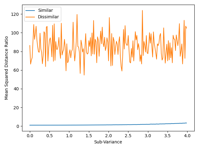
Refer to caption
Refer to caption
Figure 18: Mean Squared Distance Ratio vs. sub-variance τ2superscript𝜏2\tau^{2}. The setting is described in Section B.1.

Appendix C Complete Coarse CIFAR-10 Experiment Results

In the following sections, we provide extended experiment results. As mentioned in Section 3.2, we use learning rate in {101,102,103}superscript101superscript102superscript103\{10^{-1},10^{-2},10^{-3}\} and weight decay rate in {5×103,5×104,5×105}5superscript1035superscript1045superscript105\{5\times 10^{-3},5\times 10^{-4},5\times 10^{-5}\}. Generally, the results will be shown in a 3×3333\times 3 table, of which each grid represents the result of one hyper-parameter combination, with each row has the same learning rate and each column has the same weight decay rate.

In this section, we repeat the experiments in Section 4 with all learning rate and weight-decay rate combinations. Firstly, we present the training statistics (accuracy, loss) of all hyper-parameters in Figures 20 and 20 as an reference. It can be observed that all hyper-parameter groups achieved very low training error except the first one (weight decay = 5×1035superscript1035\times 10^{-3}, learning rate = 101superscript10110^{-1}). In fact, the last two hyper-parameter combinations (learning rate = 103superscript10310^{-3}, weight decay {5×104,5×105}absent5superscript1045superscript105\in\{5\times 10^{-4},5\times 10^{-5}\}) didn’t achieve exactly 00 training error (their training error are <0.5%absentpercent0.5<0.5\% but not exactly 00), and the other 666 hyper-parameter combinations all achieved exactly 00 training error.

Refer to caption
Figure 19: Training and test error during training.
Refer to caption
Figure 20: Training and test loss during training.

C.1 Class Distance

Here we present the visualization of the heatmap of class distance matrix D𝐷D which is defined in Section 4.1. We choose 444 epochs to show the trend during training. The results are presented in Figures 22, 22, 24 and 24, whose epoch numbers are 20,120,2402012024020,120,240 and 349349349 respectively.

Refer to caption
Figure 21: The heatmaps of class distance matrices of different hyper-parameter combinations at epoch 202020.
Refer to caption
Figure 22: The heatmaps of class distance matrices of different hyper-parameter combinations at epoch 120120120.
Refer to caption
Figure 23: The heatmaps of class distance matrices of different hyper-parameter combinations at epoch 240240240.
Refer to caption
Figure 24: The heatmaps of class distance matrices of different hyper-parameter combinations at epoch 349349349.

C.2 Visualization

In this section, we present the t-SNE visualization result of ResNet-18 on Coarse CIFAR-10 in Figures 25, 26 and 27. The results are divided into three groups, each of which has the same learning rate and the format of each group is the same as Figure 6.

Refer to caption
Refer to caption
Refer to caption
Figure 25: Visualization of last layer representations of ResNet-18 trained on Coarse CIFAR-10 with learning rate = 0.10.10.1. Each row represents a hyper-parameter combination and each column represents a super-class. The weight decay rates from top to bottom are 5×103,5×104,5×1055superscript1035superscript1045superscript1055\times 10^{-3},5\times 10^{-4},5\times 10^{-5}.
Refer to caption
Refer to caption
Refer to caption
Figure 26: Visualization of last layer representations of ResNet-18 trained on Coarse CIFAR-10 with learning rate = 0.010.010.01. Each row represents a hyper-parameter combination and each column represents a super-class. The weight decay rates from top to bottom are 5×103,5×104,5×1055superscript1035superscript1045superscript1055\times 10^{-3},5\times 10^{-4},5\times 10^{-5}.
Refer to caption
Refer to caption
Refer to caption
Figure 27: Visualization of last layer representations of ResNet-18 trained on Coarse CIFAR-10 with learning rate = 0.0010.0010.001. Each row represents a hyper-parameter combination and each column represents a super-class. The weight decay rates from top to bottom are 5×103,5×104,5×1055superscript1035superscript1045superscript1055\times 10^{-3},5\times 10^{-4},5\times 10^{-5}.

C.3 Cluster-and-Linear-Probe

The Cluster-and-Linear-Probe test results of ResNet-18 trained on Coarse CIFAR-10 with all hyper-parameter combinations are presented in Figure 29.
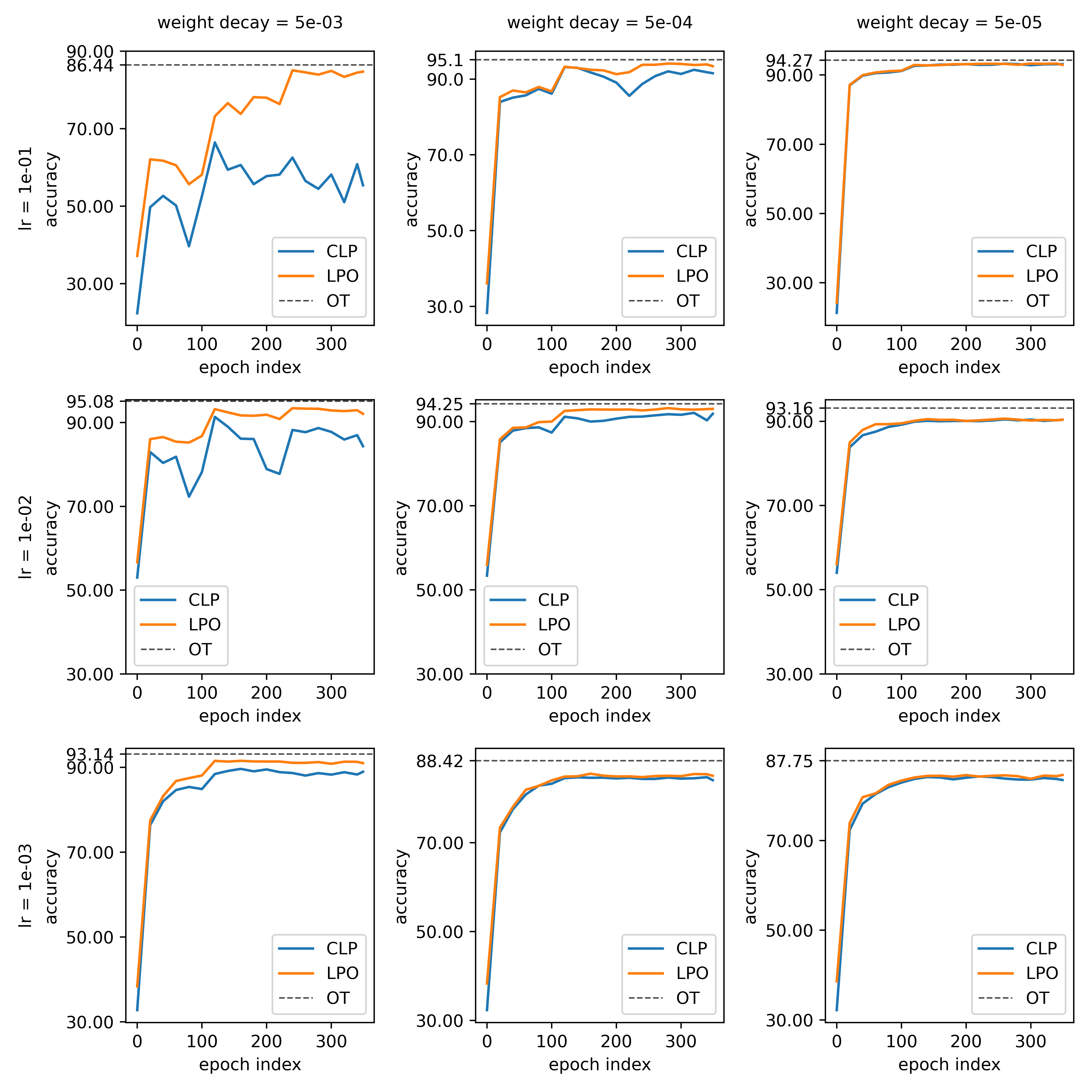
Refer to caption
Figure 28: The result of Cluster-and-Linear-Probe test. In the figure“CLP” refers to Cluster-and-Linear-Probe, “LPO” refers to linear probe with original labels and “OT’ refers to the test set accuracy of model trained on original CIFAR-10.
Refer to caption
Figure 29: The heatmaps of class distance matrices of different hyper-parameter combinations on Fine CIFAR-10 at epoch 202020.

Appendix D Complete Class Distance Result of Fine CIFAR-10

In this section, we provide the visualization of the class distance matrix of Fine CIFAR-10 with all hyper-parameter combinations, which has been partially displayed in Section 6. As before, multiple epochs during training are selected to display a evolutionary trend of the class distance matrices. The results are presented in Figures 29, 31 and 31, whose epoch numbers are 20,2002020020,200 and 350350350 respectively.

Refer to caption
Figure 30: The heatmaps of class distance matrices of different hyper-parameter combinations on Fine CIFAR-10 at epoch 200200200.
Refer to caption
Figure 31: The heatmaps of class distance matrices of different hyper-parameter combinations on Fine CIFAR-10 at epoch 350350350.

Appendix E Experiment of ResNet-18 on Coarse CIFAR-100

In this section, we report extended experiment results on Coarse CIFAR-100. The same with the case of Coarse CIFAR-10, we construct CIFAR-100 through the label coarsening process described in Section 3.2 and choose C~=20~𝐶20\tilde{C}=20, so that every 555 original classes are merged into one super-class. We repeat most of experiments in Section 4.

E.1 Class Distance

The heatmaps of distance matrices are presented in Figures 33, 33 and 36, whose epoch number are 20,2002020020,200 and 350350350 respectively.

Refer to caption
Figure 32: The heatmaps of class distance matrices of different hyper-parameter combinations on Coarse CIFAR-100 at epoch 202020.
Refer to caption
Figure 33: The heatmaps of class distance matrices of different hyper-parameter combinations on Coarse CIFAR-100 at epoch 200200200.

E.2 Visualization

In this section, we present the t-SNE visualization result of ResNet-18 on Coarse CIFAR-100. We only put the result for learning rate = 0.01 and weight decay = 1e-4 here as a demonstration in Figure 34.
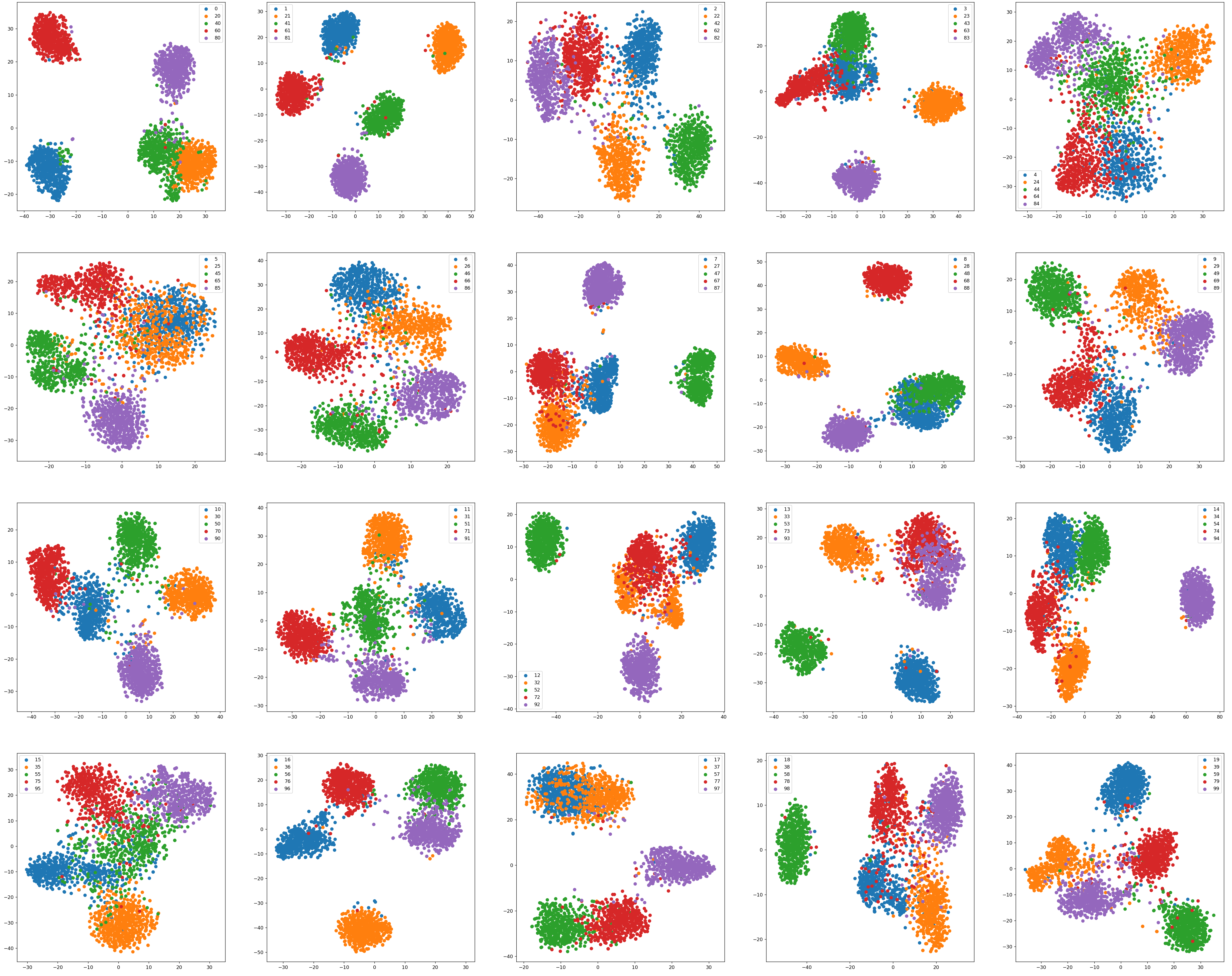
Refer to caption
Figure 34: Visualization of last layer representations of ResNet-18 trained on Coarse CIFAR-100. Each grid represents a super-class and each color in a grid represents a sub-class.

E.3 Cluster-and-Linear-Probe

Notice that we omit the visualization result of Coarse CIFAR-100 since there are too many figures. We present the Cluster-and-Linear-Probe results to reflect the clustering property of last-layer representations learned on Coarse CIFAR-100. The CLP results are presented in Figure 36.
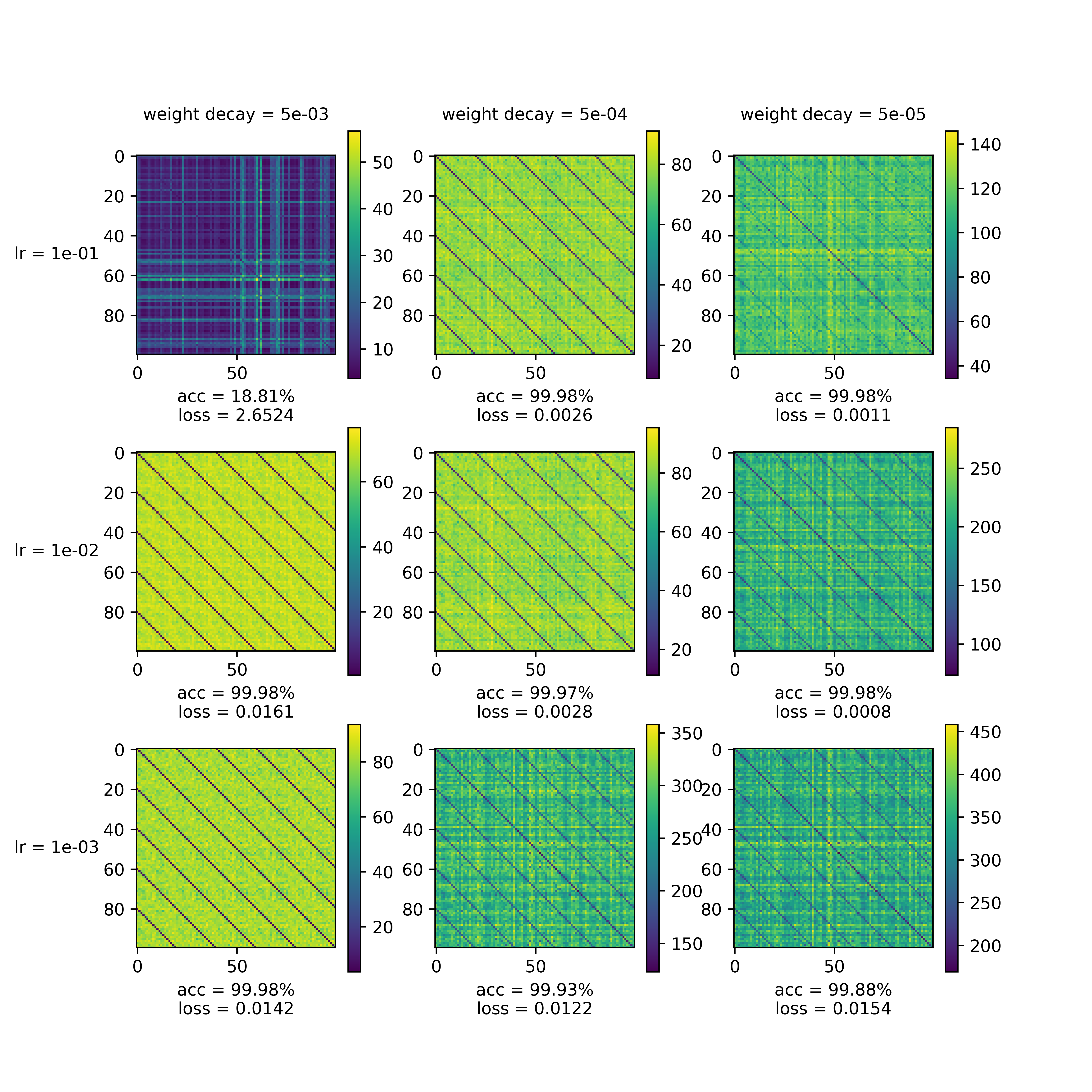
Refer to caption
Figure 35: The heatmaps of class distance matrices of different hyper-parameter combinations on Coarse CIFAR-100 at epoch 350350350.
Refer to caption
Figure 36: The result of Cluster-and-Linear-Probe test. In the figure“CLP” refers to Cluster-and-Linear-Probe, “LPO” refers to linear probe with original labels and “OT’ refers to the test set accuracy of model trained on original CIFAR-100.

Appendix F Random Coarse CIFAR-10

In this section, as mentioned in Section 3.2, we make our experiment more complete by performing a random combination of labels on CIFAR-10 rather than using a determined coarsening process as in the main paper. The dataset construction is almost the same as the process of assigning coarse labels described in Section 3.2, except here we randomly shuffle the class indices before coarsening them.

The class distance matrices of three difference epochs are shown in Figures 38, 38 and 40. From the results we can see, although there are no longer three dark lines, for each row there are generally two dark blocks, represents the original classes belongs to the same super-class, and the same observations in Section 4 can still be made here.
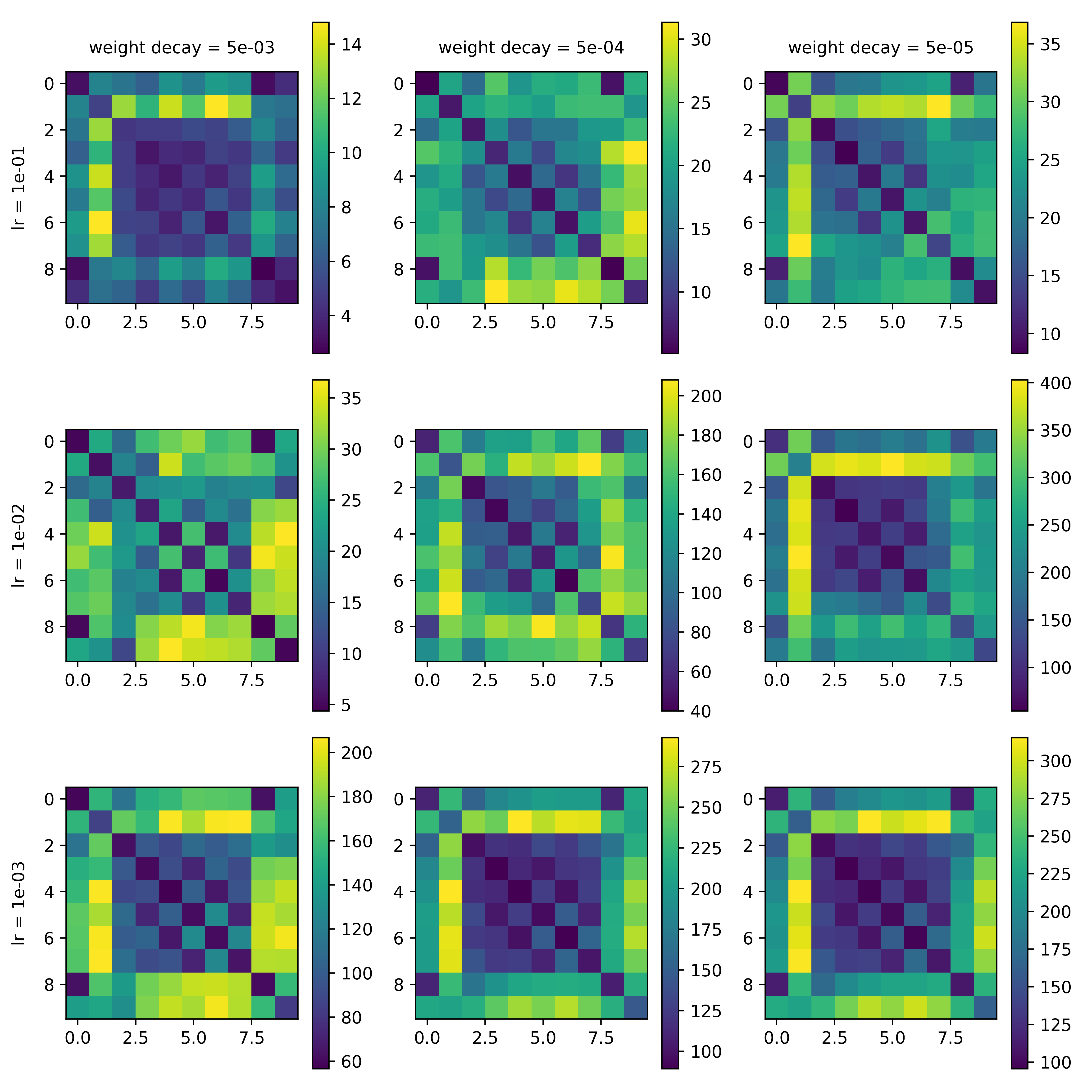
Refer to caption
Figure 37: The heatmaps of class distance matrices of different hyper-parameter combinations on Random Coarse CIFAR-10 at epoch 202020.
Refer to caption
Figure 38: The heatmaps of class distance matrices of different hyper-parameter combinations on Random Coarse CIFAR-10 at epoch 200200200.
Refer to caption
Figure 39: The heatmaps of class distance matrices of different hyper-parameter combinations on Random Coarse CIFAR-10 at epoch 350350350.
Refer to caption
Figure 40: The heatmaps of class distance matrices of different hyper-parameter combinations with DenseNet-121 on Coarse CIFAR-10 at epoch 202020.

Appendix G Experiment with DenseNet

We also perform our experiments with different neural network structures for completeness. In this section, we show the result with DenseNet-121 on Coarse CIFAR-10. The experiments with DenseNet is supportive to our observations in the main paper.

G.1 Class Distance

The class distance matrices of three epochs during training are presented in Figures 40, 42 and 42.

Refer to caption
Figure 41: The heatmaps of class distance matrices of different hyper-parameter combinations with DenseNet-121 on Coarse CIFAR-10 at epoch 202020.
Refer to caption
Figure 42: The heatmaps of class distance matrices of different hyper-parameter combinations with DenseNet-121 on Coarse CIFAR-10 at epoch 202020.

G.2 Cluster-and-Linear-Probe

The Cluster-and-Linear-Probe test results are presented in Figure 44.
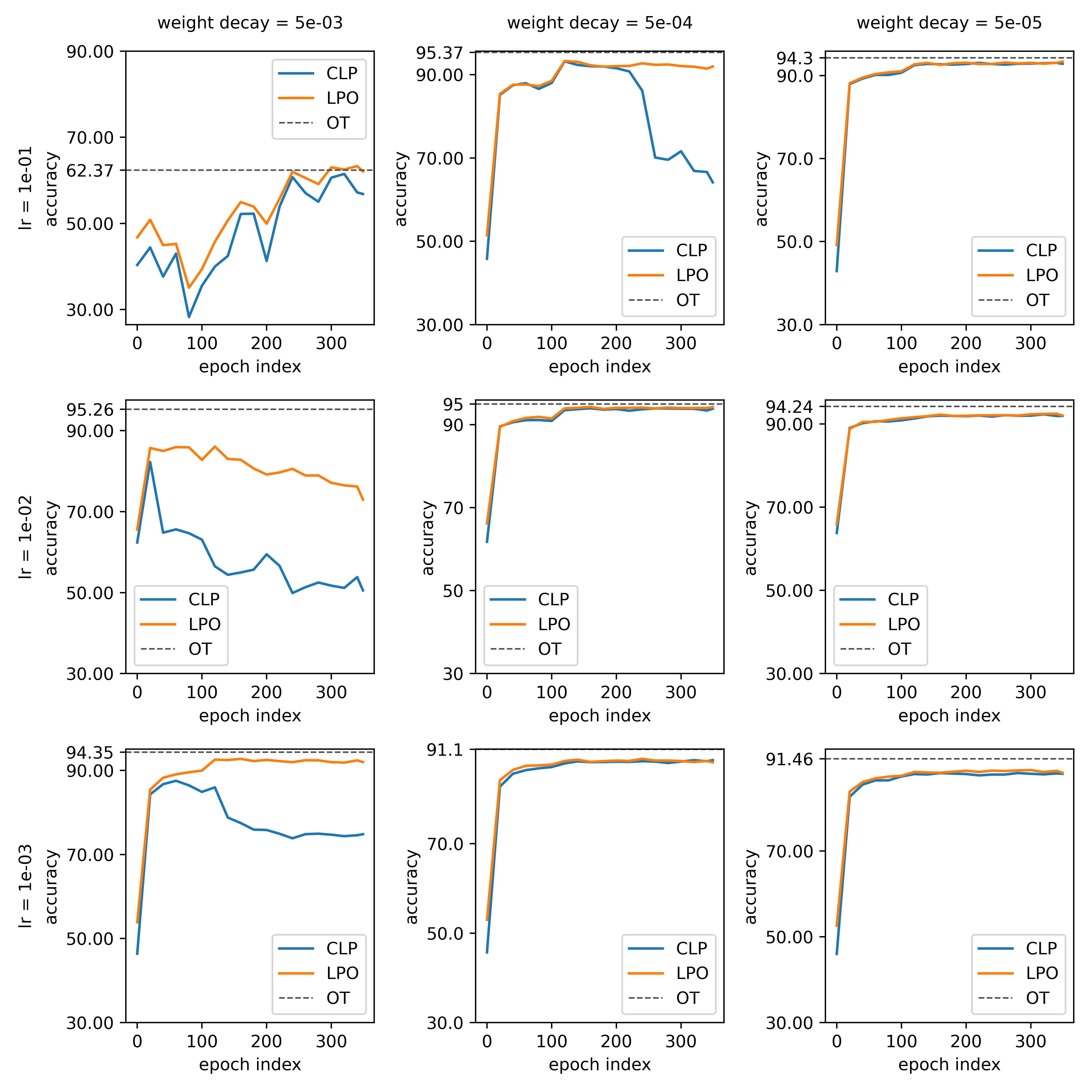
Refer to caption
Figure 43: The result of Cluster-and-Linear-Probe test with DenseNet-121. In the figure“CLP” refers to Cluster-and-Linear-Probe, “LPO” refers to linear probe with original labels and “OT’ refers to the test set accuracy of model trained on original CIFAR-10.
Refer to caption
Figure 44: The heatmaps of class distance matrices of different hyper-parameter combinations with VGG-18 on Coarse CIFAR-10 at epoch 202020.

Appendix H Experiment with VGG

We also extend our experiments to VGG-18. Interestingly, VGG to some extent is a counter example of the observations made in the main paper: it only displays Neural Collapse, and can not distinguish different original classes within one super-class, even in an early stage of training. The reason why VGG is abnormal requires further exploration.

The class distance matrices of three epochs with VGG during training are shown in Figures 44, 46 and 46. It can be observed that the three dark lines appears almost at the same time and always be of nearly the same darkness. This represents the trend predicted by Neural Collapse (Figure 4 (a)), but rejects the prediction made by (Figure 4 (b)).
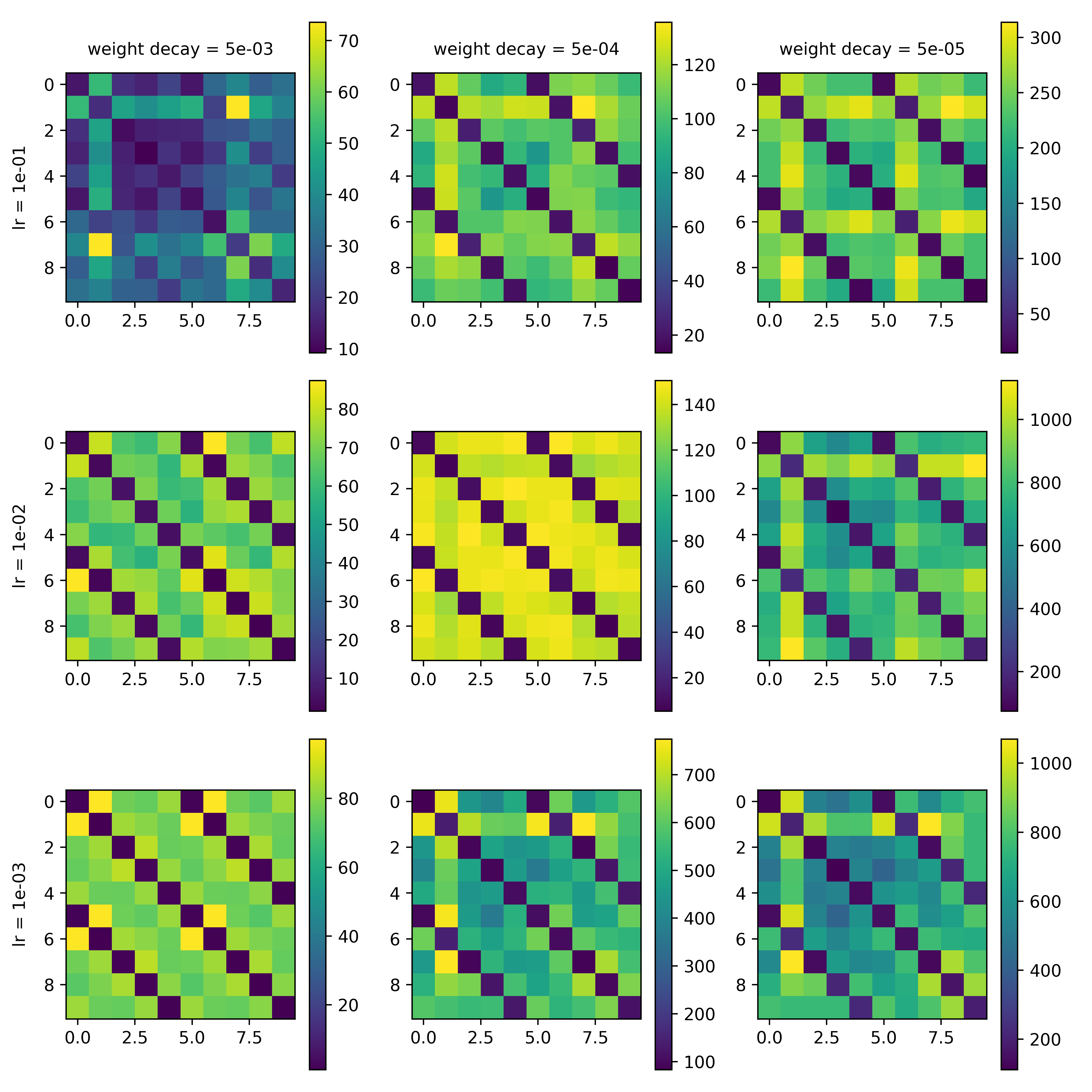
Refer to caption
Figure 45: The heatmaps of class distance matrices of different hyper-parameter combinations with VGG-18 on Coarse CIFAR-10 at epoch 200200200.
Refer to caption
Figure 46: The heatmaps of class distance matrices of different hyper-parameter combinations with VGG-18 on Coarse CIFAR-10 at epoch 350350350.