Alternative Telescopic Displacement: An Efficient Multimodal Alignment Method
Abstract
Feature alignment is the primary means of fusing multimodal data. We propose a feature alignment method that fully fuses multimodal information, which alternately shifts and expands feature information from different modalities to have a consistent representation in a feature space. The proposed method can robustly capture high-level interactions between features of different modalities, thus significantly improving the performance of multimodal learning. We also show that the proposed method outperforms other popular multimodal schemes on multiple tasks. Experimental evaluation of ETT and MIT-BIH-Arrhythmia, datasets shows that the proposed method achieves state of the art performance.
https://orcid.org/0000-0002-0551-4647
1 Introduction
Multimodal data, such as images, audio, and text, is ubiquitous in the real world. The data for each model has different eigenvectors, However, each modality has its own set of eigenvectors, which are located in different subspaces [12]. Consequently, they have different distributions and statistical properties, resulting in vectors with similar semantics being represented differently in different subspaces. Therefore, vectors with similar semantics represented in different subspaces will be completely different. This phenomenon is commonly known as the heterogeneity gap.
The heterogeneity gap is a significant issue as it can hinder the integrated use of multimodal data by subsequent machine learning modules [12]. The traditional approach to addressing this issue is to transform data from different modalities into the same vector space, for example, through feature fusion or dimensionality reduction methods. However, the disadvantage of this method is that the modal fusion is difficult, it is not easy to realize the cross-modal learning model, and the model cannot be extended to the single-modal scene [3].
Cross-modal multimedia retrieval is a popular way to solve this problem. For example, Hardoon, Szedmak and Taylor [5] map different modal data encodings to a common subspace and achieve good results on the corresponding datasets. Other researchers also achieve good results by similar methods [25] [2]. The main idea of this method is to map the features of different modes into a common low-dimensional vector space through a mapping function. In this vector space, the eigenvectors of each mode can be represented as similar vectors, which makes it convenient to perform tasks such as cross-modal retrieval and similarity calculation.
This method has been widely used in multimodal data processing and has achieved certain results. For example, in text-image retrieval, this method can be used to map text descriptions and image features into a common subspace to achieve cross-modal retrieval [3]. And in audio-image retrieval, this method can also be used to map audio and image features into a common subspace to achieve cross-modal retrieval [31] [32] [34].
However, there are some problems with this approach. For example, due to the heterogeneous gap, the mapping relationship between different modes is difficult to learn, which leads to the poor effect of the mapping function [4]. In addition, due to the high dimensionality of the feature space, the computational complexity of the learning mapping function is also high [8]. Therefore, how to effectively learn the mapping function and reduce the computational complexity is a problem that this method needs to solve.
We design a new alignment method: Alternative Telescopic Displacement(ATD), to overcome the above problems. We scale, rotate, and displace different feature spaces when fusing information features from different modalities. Displacement mapping is uncomplicated, and it can reduce the complexity of the model and prevent the gradient from disappearing. Therefore, ATD could not only fully integrate the feature information between modalities and within modalities but also could reduce overfitting and prevent gradient disappearance.
In addition, if a larger feature space is directly used to represent the features of multiple modalities, higher feature dimensions and more complex calculations will be inevitable. Before displacement mapping, we alternately select the features of one of the modalities for scaling and rotation transformation, which can reduce the dimensionality of the final alignment space. Also, we alternate between operations of stretching and rotating to add essential information about other modality features. In this way, we greatly avoid information loss.
2 Related works
Multimodal learning approach can be applied to many fields. For example, in computer vision, Velmurugan Sivakumar and Sampson [28] use multimodal medical image fusion for classification problems. They fuse multimodal medical images by shear wave transform and optimization models to obtain fused images. Their approach achieves superior performance with a fusion factor of 6.52 and a spatial frequency of 26.8. Melotti, Premebida and Goncalves [20] proposed a multimodal approach to target recognition. They integrate the RGB images captured by the camera with the LIDAR projections to handle the target recognition problem. Their method has a more accurate and robust performance compared to the unimodal approaches. Jain and Wigington [9] proposed a multimodal fusion approach for document image classification. They combine text and image features by extracting the text content through OCR technique. Such an approach can obtain 92.3% accuracy on the RVL-CDIP dataset. The multimodal approach is also applicable in the field of NLP. For instance, Jia et al. [10] pre-trained visual language dual-modality models using a noisy dataset of over 1 billion image text pairs. They achieve SOTA in a wide range of tasks. Zhang et al. [35] train image classifiers with image and text data pairs to obtain better image representations than baseline models in most cases. Liu, Wang and Li [17] integrate features from three modalities, text, audio and image, to obtain information about inter-modal consistency, which can make prediction more accurate.
In addition to the areas developed from unimodal such as computer vision and natural language processing, Multimodal models also perform well in areas such as speech recognition and video classification, which are inherently multimodal in character. Paraskevopoulos et al. [24] proposed a transformer-based combined audiovisual multimodal speech recognition model. The model uses cross-modal scaling dot product to achieve audio and visual fusion, which better adapts to the distribution characteristics of different modalities. Their experiments show that the model achieves about 50% improvement in multi-resolution convergence speed and about 18% improvement in word error rate. Eric and Hueber [29] propose a purely visual speech recognition method based on convolutional neural networks. The method uses CNN to extract features of ultrasound and video images and combines a Hidden Markov-Gaussian Mixture Model (HMM-GMM) decoder to achieve the fusion of modal information. This method achieves excellent performance in speech recognition accuracy, with an accuracy rate close to 84%. Mroueh Marcheret and Goel [23] propose a multimodal speech recognition method based on a bilinear bimodal deep neural network (DNN). The method makes full use of the correlation between audio and visual modalities to further improve speech recognition accuracy. The Phone Error Rata (PER) was reduced to 34.03%. The great results in several fields above have proven the superiority of multi-modal learning in deep learning research.
Multimodality can overcome a number of deficiencies in unimodal approaches, so multimodal approaches have superior performance over unimodal performance. A unimodal approach can only use information from one modality and cannot access information from other modalities. It may result in poor downstream task performance due to insufficient information and a lack of modal interaction [13] [15] [2]. However, multimodal methods can overcome the shortcomings of unimodal methods by integrating information from different modalities. So multimodal methods could obtain more accurate and robust results than unimodal methods. According to the survey by Baltrušaitis Ahuja and Morency [1], multimodal learning methods have been widely used in various fields such as vision, speech, and text. For example, Meng et al. [21] introduced a multimodal learning method based on deep neural networks. The method can integrate information from multiple modalities, such as vision and speech, thus improving the performance of the model. In addition, based on a survey by Mohammad Soleymani et al. [27], they conduct a series of studies on multimodal sentiment analysis tasks in social media. Their investigations find that more information and features can be obtained by analyzing and integrating information from multiple modalities, including text, images, and audio. These studies suggest that multimodal approaches can address a range of unimodality informational shortcomings and therefore perform better.
3 Multimodal model with Alternating Telescopic Displacement modules
3.1 Overview
Our bi-mode model comprises two modules: two Encoder modules that process different information modes, and an alignment module that merges the features of both modalities. The Encoder module is based on ResNet [6] and LSTM [7] network structures, while the alignment module is based on ATD. The established framework is illustrated in Figure 1 and described in detail in this paper.
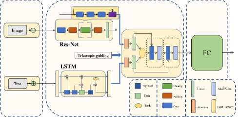
During each training process, we first feed two types of data: image and numerical data. The model then extracts numeric features and image features from the corresponding input data through two different feature extraction modules. Next, the ATD module calculates a telescopic guiding value, which is used to scale the features of one of the modalities. This allows the two sequences with the same dimension to be asymmetrically combined and then mapped to a common spatial region using displacement mapping to form a consistent representation. Finally, the output of the ATD module is processed through a fully connected layer to obtain the final output result. The algorithm based on our model is presented below:
Algorithm 1:
Input:{Image data, Numeric data}
Output :{Final-output}
I1 = Linear(Image data)
I2, V = Linear(Numeric data)
Def ATD_Block(I1,I2,V):
Guide = einsum(I1,I2)
Out = einsum(Softmax(Guide),V)
Out = Conv[Conv(Out) + I1] + I2
return Out
Img-feature = Resnet-Encoder(image);
Data-feature = LSTM-Encoder(data);
Multimodel-out = ATD_Block(Img-feature,
Data-feature,
Data-feature);
Final-output = Linear(Multimodel-out)
3.2 The Structure of the framework
In this section, we will introduce the detailed architectural design of our proposed bimodal regression network framework for numeric and image data, which includes three main modules: the image feature extraction module, the LSTM-based digital feature extraction module, and the bimodal fusion module. It should be noted that in the following equations, x1 represents numeric data and x2 represents image features.
3.3 Image feature extraction module: CNN
A Convolutional Neural Network (CNN) [14] is a type of neural network commonly used in image processing tasks. It introduces local connectivity and weight sharing between layers through convolution and pooling operations, which can significantly reduce the number of parameters in the model and improve its convergence and generalization ability. In CNN, each convolutional layer processes the input data using convolution operations. The basic idea of convolution operation is to slide a convolution kernel over each pixel of an image, multiply each element in the kernel with the corresponding pixel value in the input image, and then sum up the products to obtain the output pixel value of the convolution operation.
In this paper, we use and to represent the height and width of the input image, respectively, while and denote the corresponding dimensions of the output image. , , and represent the size, padding, and stride of the convolutional kernel used in the CNN, respectively. Specifically, during each convolution operation, the input image of size is convolved with a kernel of size , resulting in an output image of size , which can be adjusted using padding and stride .
The main structure of CNN includes convolutional layers, pooling layers and fully connected layers, and the structure of a typical CNN classification network is shown in the following figure:
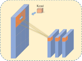
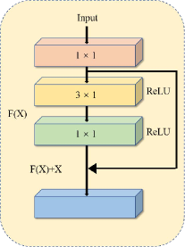
CNN can extract low or high-level features, and the level of extracted features increases with the depth of the network. The depth of the network has proven to be an important factor in achieving good performance. In our work, we intend to use a high-depth network to extract high-level features of images to obtain better classification results. However, gradient disappearance or gradient explosion becomes an obstacle for training deeper networks, which will lead to network failure to converge. The ResNet network structure can solve this problem to some extent by allowing the input information to be transferred directly to the output and added to the output layer so that the whole network only needs to learn the difference between the input and output, simplifying the learning difficulty, facilitating the convergence of the network, and protecting the integrity of the information. Presented below is the residual fork module of our image feature extraction network:
| (1) |
For m-th block of the ResNet, it can be expressed mathematically as:
| (2) | |||||
| (3) | |||||
| (4) |
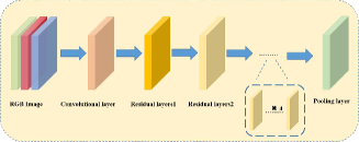
The input image feature information of residual has two propagation paths, one path is directly transferred to the output, and three convolutional layers process the other path to obtain . We use convolution and two convolution kernels in residual fork structure to extract the image features while merging with the original image feature layer information output. The output is expressed as . When the output satisfies the need of a certain task in the forward propagation process, the in the remaining residual fork layers automatically learns to become , realizing the constant mapping: , which effectively solves the degradation problem of the network. Figure 5 shows the structure of the ResNet network used in this paper:
3.4 Digital feature extraction module: LSTM
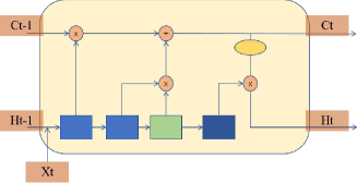
Hochreiter and Schmidhuber proposed Long Short-Term Memory [7], a network framework that can solve these problems by mitigating information loss within cells using three structures known as "gates" – Forget Gate, Output Gate and Memory Gate – composed of sigmoid neural network layers and element-wise operations to control how much information can pass through them. The strengths of an RNN mainly come from its unit-state, whereas LSTM can handle the loss of information within units through these gates to protect and maintain unit states while curbing gradient vanishing or exploding issues. Down below in this is a simple Figure 6. of the LSTM structure.
We could see this in Figure 6. The forgetting gate (left part) is responsible for forgetting a part of the memory, then the current memory is retained in the memory gate (middle part), and finally, the output gate (right part) is used in filtered and updated the memory. The parameters within these gated units can be automatically learned during training through a backpropagation algorithm.
| (5) |
Forgetting Gate: The input value and output hidden state of the previous step are combined into a single vector, then passed through the sigmoid layer . Because the sigmoid function compresses any input into the interval , the different sigmoid outputs determine how much of the information is remembered or forgotten. represents the extent of need to be forgotten.
| (6) |
Memory Gate: Use the function layer to extract the effective information of the input. refers to how much information has been extracted from the current input.
| (7) |
Using the sigmoid function to control how much of these memories are put into the cell state works as same as the Forgetting gate. represents the extent of need to be remembered.
| (8) |
The current cell state is determined by the forgetting gate and memory gate .
| (9) |
Output Gate: The input value and output hidden state of the previous step are combined into a single vector, then passed through the sigmoid layer .
| (10) |
Compress and map the current cell state to the interval through the function.
The reasons we use function in Memory gate and Output gate are to prevent the vanishing gradient problem and easy to convex optimization, converge more quickly than others.
3.4.1 Alternative Telescopic Displacement
We have extracted image and numeric features from the input data through the two modules mentioned above. In order to exploit the different features of the two modalities simultaneously, we design the Alternative Telescopic Displacement(ATD) module to fuse the features of the two modalities.
The main function of the ATD module is to alternately scale, rotate, and shift the eigenmatrices of the two modes. These could prevent us from getting a public representation space of a huge scale and getting stuck in more complex computations. Moreover, it can maintain a relatively simple mapping relationship with the original feature space. It works as follows:
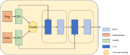
We perform Layernorm processing on the image and the digital features obtained from the two unimodal channels to obtain the normalized results.
| (11) | |||||
| (12) |
Then we alternately select the feature matrix of one of the modalities and perform scaling and rotation transformations to reduce the dimension while keeping the feature representation unchanged.
Get the guide() of image identity and series identity by scaling the dot product. The value of will be updated with the weight value update after backpropagation during training, meaning that the proportion of image and time-series data is different when each training is passed to the ATD module. The entire network will adjust the value of with more training errors until the performance reaches the optimum.
| (13) |
Computes the operation of taking the maximum value of Guide along the last dimension. This maximum value is then subtracted from each element of the Guide matrix.
| (14) |
denotes the th sample in the batch, denotes the th head, and and denote the positions in the sequence, respectively. Finally, each element in is compressed to the interval , which ensures numerical stability after the softmax operation.
The Guide obtained through scaled dot-product is substituted into the Softmax function to obtain the ATD weights.
| (15) |
The output is the result of the operation of value and ATD weights:
| (16) |
Select the feature matrix of a single modality and apply scaling and rotation transformations to reduce the dimensionality while maintaining the feature representation unchanged.
| (17) | |||||
| (18) |
Finally, the normalized original features are displacement mapped with the interaction output of the same dimension.
4 Experiments and Results
We selected two different datasets for experiments, proving that the ATD module is not limited to a single specified task.
Besides, to prove that our experiments with multimodal data are adequate, we also conduct experiments with single modality data of the two datasets, respectively.
Finally, to verify that our proposed ATD module is a better alignment method, we use two other alignment methods to replace the ATD module in our model for experiments.
4.1 Datasets
ETT (electric Transformer Temperature) [36]: This dataset records transformer temperature data for two years, and all data is divided into 1-hour classes. Each data point has a target temperature value and six power load characteristics.
The MIT-BIH Arrhythmia Database [22]: This dataset contains 48 excerpts of two-channel ambulatory ECG recordings taken from 47 subjects studied between 1975 and 1979 by the BIH Arrhythmia Laboratory. Twenty-three recordings were randomly selected from 4000 patients aged 24-30. Hour Holter recordings were collected from a mixed population of inpatients (approximately 60%) and outpatients (approximately 40%) at Beth Israel Hospital in Boston; the remainder 25 records were selected from the same group to include less common but clinically significant arrhythmias that would not be well represented in a small random sample.
We perform regression tasks on the ETT dataset and classification tasks on the MIT-BIH Arrhythmia dataset.
4.2 Comparison with other methods
Table 1 shows that the performance of our proposed method on the ETT dataset is better than the others.
| Measurement metrics | ||
|---|---|---|
| Method | MAE | MSE |
| NLinear[33] | 0.226 | 0.080 |
| FiLM[37] | 0.240 | 0.090 |
| SCINet[18] | 0.127 | 0.029 |
| ATD (our) | 0.058 | 0.006 |
Experimental results on the ETT dataset show that our model has better performance. Compared with previous SOTA results, our results have the minimum MAE and MSE, meaning our model has more minor errors.
Table 2 shows that the performance of our proposed method on MIT-BIH-Arrhythmia dataset is state of the art.
5 Ablation studies
5.1 Single mode results
We conduct experiments with unimodal data, and the results show that our ATD multimodal model has better performance. Table 3 shows that forecasting using only numerical data of ETT can not perform as well as ATD multimodal.
| Measurement metrics | ||
|---|---|---|
| Method | MAE | MSE |
| Numerical only | 0.187 | 0.0298 |
| ATD (multimodal) | 0.058 | 0.006 |
Table 4 shows the classification results using image and time-series signal data from the MIT-BIH Arrhythmia dataset. The results of ATD multimodal classification are better.
| Measurement metrics | ||
|---|---|---|
| Method | Accuracy | F1 |
| Image only | 0.518 | 0.479 |
| Time-series only | 0.858 | 0.893 |
| ATD (multimodal) | 0.989 | 0.982 |
5.2 Results using other alignment methods
LMF [19] and Cross-attention [16] are popular multimodal alignment methods. We use these two modules to replace the ATD module in our model for experiments.
Table 5 and Table 6 present the results of experiments with other alignment methods.
| Measurement metrics | ||||
|---|---|---|---|---|
| Dataset | MAE | MSE | Accuracy | F1 |
| ETT | 0.337 | 0.116 | - | - |
| MIT-BIH Arrhythmia | - | - | 0.912 | 0.905 |
| Measurement metrics | ||||
|---|---|---|---|---|
| Dataset | MAE | MSE | Accuracy | F1 |
| ETT | 0.187 | 0.086 | - | - |
| MIT-BIH Arrhythmia | - | - | 0.942 | 0.931 |
Compared with different alignment methods, ATD has apparent advantages in performance.
From the above table, compared with different alignment methods, ATD has apparent advantages in performance.
ATD can fully fuse the information inside and outside the modal. Therefore, the experimental results of the ATD model on the ETT dataset and MIT-BIH Arrhythmia dataset have achieved better performance.
6 Analysis and Discussion
6.1 Greater performance
Compared with LMF, the performance of the model using ATD on the ETT dataset is improved by 82.8% (MAE) and 48.3% (MSE), and the performance of the model using ATD on the MIT-BIH-Arrythmia dataset is improved by 8.4% (Acc) and 8.5% (F1 score). Compared with ATD, the performance of the model using ATD on the ETT dataset is improved by 31.0% (MAE) and 7.0% (MSE), and the performance of the model using ATD on the MIT-BIH-Arrythmia dataset is improved by 5.0% (Acc) and 5.5% (F1 score).
Compared with the existing methods, ATD performs better, and ATD is more environmentally friendly. It has fewer parameters, is easier to train, and deploy on a personal PC or even some portable device.
6.2 More environmentally friendly and easy to use
The ATD module can significantly reduce the number of parameters of the overall model. Under the premise of using CNN and LSTM as encoders, The number of parameters of the model using ATD for modal alignment is only 70 million. The parameters of the model using LMF and cross-attention are 71 million and 160 million, respectively. Compared with LMF, ATD reduces the model parameters by 1 million, and the parameter reduction ratio is 1.4%. Compared with cross-attention, ATD reduces the model parameters by 90 million, and the parameter reduction ratio is 56.3%. With transformer and version-transformer as the encoder, The number of model parameters using ATD for modal alignment is 282 million, and the number of model parameters using LMF and cross-attention is 283 million and 370 million, respectively. Compared with LMF, ATD reduces the model by 1 million parameters with a parameter reduction ratio of 0.6%, and compared with cross-attention, ATD reduces the model by 88 million parameters with a parameter reduction ratio of 24%.
| Alignment methods | |||
|---|---|---|---|
| Encoders | ATD | LMF | Cross-attention |
| Cnn and Lstm | 70 million | 71 million | 160 million |
| Transformer and VIT | 282 million | 283 million | 370 million |
7 Conclusions and future works
This paper proposes a new method for fusing feature information from multiple modalities: Alternative Telescopic Displacement (ATD). ATD alternately selects the feature matrix of each mode and performs scaling, rotation and displacement transformations. It can align the feature information of multiple modalities in a common subspace. We use one multimodal model with ATD to achieve the best performance on two datasets.
In future works, we will work on improving the compatibility of the ATD module to ensure that it can efficiently work with any neural network architecture. In addition, we plan to apply the ATD module in more complex multimodal learning, such as multimodal unsupervised tasks.
References
- [1] Tadas Baltrušaitis, Chaitanya Ahuja, and Louis-Philippe Morency, ‘Multimodal Machine Learning: A Survey and Taxonomy’, IEEE Transactions on Pattern Analysis and Machine Intelligence, 41(2), 423–443, (February 2019). Conference Name: IEEE Transactions on Pattern Analysis and Machine Intelligence.
- [2] Yixuan Chen, Dongsheng Li, Peng Zhang, Jie Sui, Qin Lv, Lu Tun, and Li Shang, ‘Cross-modal Ambiguity Learning for Multimodal Fake News Detection’, in Proceedings of the ACM Web Conference 2022, WWW ’22, pp. 2897–2905, New York, NY, USA, (April 2022). Association for Computing Machinery.
- [3] Jaemin Cho, Jie Lei, Hao Tan, and Mohit Bansal, ‘Unifying Vision-and-Language Tasks via Text Generation’, in Proceedings of the 38th International Conference on Machine Learning, pp. 1931–1942. PMLR, (July 2021). ISSN: 2640-3498.
- [4] Wenzhong Guo, Jianwen Wang, and Shiping Wang, ‘Deep Multimodal Representation Learning: A Survey’, IEEE Access, 7, 63373–63394, (2019). Conference Name: IEEE Access.
- [5] David R. Hardoon, Sandor Szedmak, and John Shawe-Taylor, ‘Canonical Correlation Analysis: An Overview with Application to Learning Methods’, Neural Computation, 16(12), 2639–2664, (December 2004). Conference Name: Neural Computation.
- [6] Kaiming He, Xiangyu Zhang, Shaoqing Ren, and Jian Sun, ‘Deep Residual Learning for Image Recognition’, pp. 770–778, (2016).
- [7] Sepp Hochreiter and Jürgen Schmidhuber, ‘Long Short-Term Memory’, Neural Computation, 9(8), 1735–1780, (November 1997). Conference Name: Neural Computation.
- [8] Michael E. Houle, Hans-Peter Kriegel, Peer Kröger, Erich Schubert, and Arthur Zimek, ‘Can Shared-Neighbor Distances Defeat the Curse of Dimensionality?’, in Scientific and Statistical Database Management, eds., Michael Gertz and Bertram Ludäscher, Lecture Notes in Computer Science, pp. 482–500, Berlin, Heidelberg, (2010). Springer.
- [9] Rajiv Jain and Curtis Wigington, ‘Multimodal Document Image Classification’, in 2019 International Conference on Document Analysis and Recognition (ICDAR), pp. 71–77, (September 2019). ISSN: 2379-2140.
- [10] Chao Jia, Yinfei Yang, Ye Xia, Yi-Ting Chen, Zarana Parekh, Hieu Pham, Quoc Le, Yun-Hsuan Sung, Zhen Li, and Tom Duerig, ‘Scaling Up Visual and Vision-Language Representation Learning With Noisy Text Supervision’, in Proceedings of the 38th International Conference on Machine Learning, pp. 4904–4916. PMLR, (July 2021). ISSN: 2640-3498.
- [11] Serkan Kiranyaz, Turker Ince, and Moncef Gabbouj, ‘Real-time patient-specific ecg classification by 1-d convolutional neural networks’, IEEE Transactions on Biomedical Engineering, 63(3), 664–675, (2015).
- [12] Dana Lahat, Tülay Adali, and Christian Jutten, ‘Multimodal Data Fusion: An Overview of Methods, Challenges, and Prospects’, Proceedings of the IEEE, 103(9), 1449–1477, (September 2015). Conference Name: Proceedings of the IEEE.
- [13] Claudia Lappe, Sibylle C. Herholz, Laurel J. Trainor, and Christo Pantev, ‘Cortical Plasticity Induced by Short-Term Unimodal and Multimodal Musical Training’, Journal of Neuroscience, 28(39), 9632–9639, (September 2008). Publisher: Society for Neuroscience Section: Articles.
- [14] Yann LeCun, Léon Bottou, Yoshua Bengio, and Patrick Haffner, ‘Gradient-based learning applied to document recognition’, Proceedings of the IEEE, 86(11), 2278–2324, (1998).
- [15] Tao Liang, Guosheng Lin, Mingyang Wan, Tianrui Li, Guojun Ma, and Fengmao Lv, ‘Expanding Large Pre-Trained Unimodal Models With Multimodal Information Injection for Image-Text Multimodal Classification’, pp. 15492–15501, (2022).
- [16] Hezheng Lin, Xing Cheng, Xiangyu Wu, and Dong Shen, ‘Cat: Cross attention in vision transformer’, in 2022 IEEE International Conference on Multimedia and Expo (ICME), pp. 1–6. IEEE, (2022).
- [17] Hui Liu, Wenya Wang, and Haoliang Li. Towards Multi-Modal Sarcasm Detection via Hierarchical Congruity Modeling with Knowledge Enhancement, October 2022. arXiv:2210.03501 [cs].
- [18] Minhao Liu, Ailing Zeng, Muxi Chen, Zhijian Xu, Qiuxia Lai, Lingna Ma, and Qiang Xu, ‘Scinet: time series modeling and forecasting with sample convolution and interaction’, Advances in Neural Information Processing Systems, 35, 5816–5828, (2022).
- [19] Zhun Liu, Ying Shen, Varun Bharadhwaj Lakshminarasimhan, Paul Pu Liang, Amir Zadeh, and Louis-Philippe Morency, ‘Efficient low-rank multimodal fusion with modality-specific factors’, arXiv preprint arXiv:1806.00064, (2018).
- [20] Gledson Melotti, Cristiano Premebida, and Nuno Gonçalves, ‘Multimodal Deep-Learning for Object Recognition Combining Camera and LIDAR Data’, in 2020 IEEE International Conference on Autonomous Robot Systems and Competitions (ICARSC), pp. 177–182, (April 2020).
- [21] Hongying Meng, Di Huang, Heng Wang, Hongyu Yang, Mohammed AI-Shuraifi, and Yunhong Wang, ‘Depression recognition based on dynamic facial and vocal expression features using partial least square regression’, in Proceedings of the 3rd ACM international workshop on Audio/visual emotion challenge, AVEC ’13, pp. 21–30, New York, NY, USA, (October 2013). Association for Computing Machinery.
- [22] George B Moody and Roger G Mark, ‘The impact of the mit-bih arrhythmia database’, IEEE engineering in medicine and biology magazine, 20(3), 45–50, (2001).
- [23] Youssef Mroueh, Etienne Marcheret, and Vaibhava Goel, ‘Deep multimodal learning for Audio-Visual Speech Recognition’, in 2015 IEEE International Conference on Acoustics, Speech and Signal Processing (ICASSP), pp. 2130–2134, (April 2015). ISSN: 2379-190X.
- [24] Georgios Paraskevopoulos, Srinivas Parthasarathy, Aparna Khare, and Shiva Sundaram. Multiresolution and Multimodal Speech Recognition with Transformers, April 2020. arXiv:2004.14840 [cs, eess, stat].
- [25] Yuxin Peng, Jinwei Qi, and Yuxin Yuan, ‘Modality-Specific Cross-Modal Similarity Measurement With Recurrent Attention Network’, IEEE Transactions on Image Processing, 27(11), 5585–5599, (November 2018). Conference Name: IEEE Transactions on Image Processing.
- [26] Abdelrahman M Shaker, Manal Tantawi, Howida A Shedeed, and Mohamed F Tolba, ‘Generalization of convolutional neural networks for ecg classification using generative adversarial networks’, IEEE Access, 8, 35592–35605, (2020).
- [27] Mohammad Soleymani, David Garcia, Brendan Jou, Björn Schuller, Shih-Fu Chang, and Maja Pantic, ‘A survey of multimodal sentiment analysis’, Image and Vision Computing, 65, 3–14, (September 2017).
- [28] Velmurugan Subbiah Parvathy, Sivakumar Pothiraj, and Jenyfal Sampson, ‘Optimal Deep Neural Network model based multimodality fused medical image classification’, Physical Communication, 41, 101119, (August 2020).
- [29] Eric Tatulli and Thomas Hueber, ‘Feature extraction using multimodal convolutional neural networks for visual speech recognition’, in 2017 IEEE International Conference on Acoustics, Speech and Signal Processing (ICASSP), pp. 2971–2975, (March 2017). ISSN: 2379-190X.
- [30] Mehmet Yamaç, Mert Duman, İlke Adalıoğlu, Serkan Kiranyaz, and Moncef Gabbouj, ‘A personalized zero-shot ecg arrhythmia monitoring system: From sparse representation based domain adaption to energy efficient abnormal beat detection for practical ecg surveillance’, arXiv preprint arXiv:2207.07089, (2022).
- [31] Rui Yang, Shuang Wang, Yingzhi Sun, Huan Zhang, Yu Liao, Yu Gu, Biao Hou, and Licheng Jiao, ‘Multimodal fusion remote sensing image–audio retrieval’, IEEE Journal of Selected Topics in Applied Earth Observations and Remote Sensing, 15, 6220–6235, (2022).
- [32] Zhiqiang Yuan, Wenkai Zhang, Kun Fu, Xuan Li, Chubo Deng, Hongqi Wang, and Xian Sun, ‘Exploring a fine-grained multiscale method for cross-modal remote sensing image retrieval’, arXiv preprint arXiv:2204.09868, (2022).
- [33] Ailing Zeng, Muxi Chen, Lei Zhang, and Qiang Xu, ‘Are transformers effective for time series forecasting?’, arXiv preprint arXiv:2205.13504, (2022).
- [34] Hong Zhang, Yueting Zhuang, and Fei Wu, ‘Cross-modal correlation learning for clustering on image-audio dataset’, in Proceedings of the 15th ACM international conference on Multimedia, pp. 273–276, (2007).
- [35] Yuhao Zhang, Hang Jiang, Yasuhide Miura, Christopher D. Manning, and Curtis P. Langlotz. Contrastive Learning of Medical Visual Representations from Paired Images and Text, September 2022. arXiv:2010.00747 [cs].
- [36] Haoyi Zhou, Shanghang Zhang, Jieqi Peng, Shuai Zhang, Jianxin Li, Hui Xiong, and Wancai Zhang, ‘Informer: Beyond efficient transformer for long sequence time-series forecasting’, in The Thirty-Fifth AAAI Conference on Artificial Intelligence, AAAI 2021, Virtual Conference, volume 35, pp. 11106–11115. AAAI Press, (2021).
- [37] Tian Zhou, Ziqing Ma, Qingsong Wen, Liang Sun, Tao Yao, Wotao Yin, Rong Jin, et al., ‘Film: Frequency improved legendre memory model for long-term time series forecasting’, Advances in Neural Information Processing Systems, 35, 12677–12690, (2022).