The Expressive Leaky Memory Neuron:
an Efficient and Expressive Phenomenological
Neuron Model Can Solve Long-Horizon Tasks

Abstract

Biological cortical neurons are remarkably sophisticated computational devices, temporally integrating their vast synaptic input over an intricate dendritic tree, subject to complex, nonlinearly interacting internal biological processes. A recent study proposed to characterize this complexity by fitting accurate surrogate models to replicate the input-output relationship of a detailed biophysical cortical pyramidal neuron model and discovered it needed temporal convolutional networks (TCN) with millions of parameters. Requiring these many parameters, however, could be the result of a misalignment between the inductive biases of the TCN and cortical neuron’s computations. In light of this, and with the aim to explore the computational implications of leaky memory units and nonlinear dendritic processing, we introduce the Expressive Leaky Memory (ELM) neuron model, a biologically inspired phenomenological model of a cortical neuron. Remarkably, by exploiting a few such slowly decaying memory-like hidden states and two-layered nonlinear integration of synaptic input, our ELM neuron can accurately match the aforementioned input-output relationship with under ten-thousand trainable parameters. To further assess the computational ramifications of our neuron design, we evaluate on various tasks with demanding temporal structures, including the Long Range Arena (LRA) datasets, as well as a novel neuromorphic dataset based on the Spiking Heidelberg Digits dataset (SHD-Adding). Leveraging a larger number of memory units with sufficiently long timescales, and correspondingly sophisticated synaptic integration, the ELM neuron proves to be competitive on both datasets, reliably outperforming the classic Transformer or Chrono-LSTM architectures on latter, even solving the Pathfinder-X task with over $70\%$ accuracy (16k context length). These findings indicate the importance of inductive biases for efficient surrogate neuron models and the potential for biologically motivated models to enhance performance in challenging machine learning tasks.

1 Introduction

The human brain has impressive computational capabilities, yet the precise mechanisms underpinning them remain largely undetermined. Two complementary directions are pursued in search of mechanisms for brain computations. On the one hand, many researchers investigate how these capabilities could arise from the collective activity of neurons connected into a complex network structure Maass (1997); Gerstner & Kistler (2002); Grüning & Bohte (2014), where individual neurons might be as basic as leaky integrators or ReLU neurons. On the other hand, it has been proposed that the intrinsic computational power possessed by individual neurons Koch (1997); Koch & Segev (2000); Silver (2010) contributes a significant part to the computations.

Even though most work focuses on the former hypothesis, an increasing amount of evidence indicates that cortical neurons are remarkably sophisticated Silver (2010); Gidon et al. (2020); Larkum (2022), even comparable to expressive multilayered artificial neural networks Poirazi et al. (2003); Jadi et al. (2014); Beniaguev et al. (2021); Jones & Kording (2021), and capable of discriminating between dozens to hundreds of input patterns Gütig & Sompolinsky (2006); Hawkins & Ahmad (2016); Moldwin & Segev (2020). Numerous biological mechanisms, such as complex ion channel dynamics (e.g. NMDA nonlinearity Major et al. (2013); Lafourcade et al. (2022); Tang et al. (2023)), plasticity on various and especially longer timescales (e.g. slow spike frequency adaptation Kobayashi et al. (2009); Bellec et al. (2020)), the intricate cell morphology (e.g. nonlinear integration by dendritic tree Stuart & Spruston (2015); Poirazi & Papoutsi (2020); Larkum (2022)), and their interactions, have been identified to contribute to their complexity.

Detailed biophysical models of cortical neurons aim to capture this inherent complexity through high-fidelity simulations Hay et al. (2011); Herz et al. (2006); Almog & Korngreen (2016). However, they require a lot of computing resources to run and typically operate at a very fine level of granularity that does not facilitate the extraction of higher-level insights into the neuron’s computational principles. A promising approach to deriving such higher-level insights from simulations is through the training of surrogate phenomenological neuron models. These models are designed to replicate the output of high-fidelity biophysical simulations but use simplified interpretable components. This approach was employed, for example, to model computation in the dendritic tree via simple two-layer ANN Poirazi et al. (2003); Tzilivaki et al. (2019); Ujfalussy et al. (2018). Building on this line of research, a recent study by Beniaguev et al. (2021) developed a temporal convolutional network to capture the spike-level input/output (I/O) relationship with millisecond precision, accounting for the complexity of integrating diverse synaptic input across the entirety of the dendritic tree of a high-fidelity biophysical neuron model. It was found that a highly expressive temporal convolutional network with millions of parameters was essential to reproduce the aforementioned I/O relationship.

In this work, we propose that a model equipped with appropriate inductive biases that align with the high-level computational principles of a cortical neuron should be capable of capturing the I/O relationship using a substantially smaller model size. To achieve this, a model would likely need to account for multiple mechanisms of neural expressivity and judiciously allocate computational resources and parameters in rough analogy to biological neurons. Should such a construction be possible, the requisite design choices may yield insights into principles of neural computation at the conceptual level. We proceed to design the Expressive Leaky Memory (ELM) neuron model (see Figure 1), a biologically inspired phenomenological model of a cortical neuron. While biologically inspired, low-level biological processes are abstracted away for computational efficiency, and consequently individual parameters of the ELM neuron are not designed for direct biophysical interpretation. Nevertheless, model ablations can provide conceptual insights into the computational components required to emulate the cortical input/output relationship. The ELM neuron functions as a recurrent cell and can be conveniently used as a drop-in replacement for LSTMs Hochreiter & Schmidhuber (1997).

Our experiments show that a variant of the ELM neuron is expressive enough to accurately match the spike level I/O of a detailed biophysical model of a layer 5 pyramidal neuron at a millisecond temporal resolution with merely a few thousand parameters, in stark contrast to the millions of parameters required by temporal convolutional networks. Conceptually, we find accurate surrogate models to require multiple memory-like hidden states with longer timescales and highly nonlinear synaptic integration. To explore the implications of neuron-internal timescales and sophisticated synaptic integration into multiple memory units, we first probe its temporal information integration capabilities on a challenging biologically inspired neuromorphic dataset requiring the addition of spike-encoded spoken digits. We find that the ELM neuron can outperform classic LSTMs leveraging a sufficient number of slowly decaying memory and highly nonlinear synaptic integration. We subsequently evaluate the ELM neuron on three well-established long sequence modeling LRA benchmarks from the machine learning literature, including the notoriously challenging Pathfinder-X task, where it achieves over $70\%$ accuracy but many transformer-based models struggle to learn at all.

Our contributions are the following.

1. We propose the phenomenological Expressive Leaky Memory (ELM) neuron model, a recurrent cell architecture inspired by biological cortical neuron.

2. The ELM neuron efficiently learns the input/output relationship of a sophisticated biophysical model of a cortical neuron, indicating it’s inductive biases to be well aligned.

3. The ELM neuron facilitates the formulation and validation of hypotheses regarding the underlying computations of biological neurons.

4. Lastly, we demonstrate the impressive long-sequence processing capabilities of the ELM, implicating the utility of leaky memory units and nonlinear dendritic processing, and suggesting broader applicability of ELM-like architectures in machine learning applications.

2 The Expressive Leaky Memory Neuron

(a) A Cortical Neuron

(b) The ELM Neuron Architecture

$$\begin{split}{\color[rgb]{0.00390625,0.44921875,0.69921875}\bm{\kappa_{m}}}&=\exp(\nicefrac{{-\Delta t}}{{{\color[rgb]{0.00390625,0.44921875,0.69921875}\bm{\tau_{m}}}}})\\ {\color[rgb]{0.0078125,0.62109375,0.44921875}\bm{\kappa_{s}}}&=\exp(\nicefrac{{-\Delta t}}{{{\color[rgb]{0.0078125,0.62109375,0.44921875}\bm{\tau_{s}}}}})\\ {\color[rgb]{0.0078125,0.62109375,0.44921875}\bm{s_{t}}}&={\color[rgb]{0.0078125,0.62109375,0.44921875}\bm{\kappa_{s}}}\odot{\color[rgb]{0.0078125,0.62109375,0.44921875}\bm{s_{t-1}}}+{\color[rgb]{0.0078125,0.62109375,0.44921875}\bm{w_{s}}}\odot\bm{x_{t}}\\ {\color[rgb]{0.87109375,0.5625,0.01953125}\bm{\Delta m_{t}}}&=\tanh(\text{MLP}_{{\color[rgb]{0.87109375,0.5625,0.01953125}\bm{w_{p}}}}([{\color[rgb]{0.0078125,0.62109375,0.44921875}\bm{s_{t}}},{\color[rgb]{0.00390625,0.44921875,0.69921875}\bm{\kappa_{m}}}\odot{\color[rgb]{0.00390625,0.44921875,0.69921875}\bm{m_{t-1}}}]))\\ {\color[rgb]{0.00390625,0.44921875,0.69921875}\bm{m_{t}}}&={\color[rgb]{0.00390625,0.44921875,0.69921875}\bm{\kappa_{m}}}\odot{\color[rgb]{0.00390625,0.44921875,0.69921875}\bm{m_{t-1}}}+{\color[rgb]{0.87109375,0.5625,0.01953125}\lambda}(1-{\color[rgb]{0.00390625,0.44921875,0.69921875}\bm{\kappa_{m}}})\odot{\color[rgb]{0.87109375,0.5625,0.01953125}\bm{\Delta m_{t}}}\\ {\color[rgb]{0.80078125,0.46875,0.73828125}\bm{y_{t}}}&={\color[rgb]{0.80078125,0.46875,0.73828125}\bm{w_{y}}}\cdot{\color[rgb]{0.00390625,0.44921875,0.69921875}\bm{m_{t}}}\end{split}$$ (1)

(c) The ELM Neuron Equations

Figure 1: The biologically motivated Expressive Leaky Memory (ELM) neuron model. The architecture can be divided into the following components; the input current synapse dynamics, the integration mechanism dynamics, the leaky memory dynamics, and the output dynamics. a) Sketch of a biological cortical pyramidal neuron segmented into the analogous architectural components using the corresponding colors. b) Schematics of the ELM neuron architecture, component-wise colored accordingly. c) The ELM neuron equations, where $\bm{x_{t}}\in\mathbb{R}^{d_{s}}$ is the input at time $t$, $\Delta t\in\mathbb{R}^{+}$ the fictitious elapsed time in milliseconds between two consecutive inputs $\bm{x_{t-1}}$ and $\bm{x_{t}}$ , ${\color[rgb]{0.00390625,0.44921875,0.69921875}\bm{m}}\in\mathbb{R}^{d_{m}}$ are memory units, ${\color[rgb]{0.0078125,0.62109375,0.44921875}\bm{s}}\in\mathbb{R}^{d_{s}}$ the synapse currents (traces), ${\color[rgb]{0.00390625,0.44921875,0.69921875}\bm{\tau_{m}}}\in\mathbb{R^{+}}^{d_{m}}$ and ${\color[rgb]{0.0078125,0.62109375,0.44921875}\bm{\tau_{s}}}\in\mathbb{R^{+}}^{d_{s}}$ their respective timescales in milliseconds, ${\color[rgb]{0.0078125,0.62109375,0.44921875}\bm{w_{s}}}\in\mathbb{R^{+}}^{d_{s}}$ are synapse weights, ${\color[rgb]{0.87109375,0.5625,0.01953125}\bm{w_{p}}}$ the weights of a Multilayer Perceptron (MLP) with $l_{\mathrm{mlp}}$ hidden layers of size $d_{\mathrm{mlp}}$, ${\color[rgb]{0.80078125,0.46875,0.73828125}\bm{w_{y}}}\in\mathbb{R}^{d_{o}\times d_{m}}$ the output weights, ${\color[rgb]{0.87109375,0.5625,0.01953125}\lambda}\in\mathbb{R^{+}}$ a scaling factor for the delta memory ${\color[rgb]{0.87109375,0.5625,0.01953125}\Delta m_{t}}\in\mathbb{R}^{d_{m}}$, and ${\color[rgb]{0.80078125,0.46875,0.73828125}\bm{y}}\in\mathbb{R}^{d_{o}}$ the output.

In this section, we discuss the design of the Expressive Leaky Memory (ELM) neuron. It’s architecture is engineered to efficiently capture sophisticated cortical neuron computations. Abstracting mechanistic neuronal implementation details away, we resort to an overall recurrent cell architecture with biologically motivated computational components. This design approach emphasizes conceptual over mechanistic insight into cortical neuron computations.

The current synapse dynamics.

Neurons receive inputs at their synapses in form of sparse binary events known as spikes Kandel et al. (2000). While the Excitatory/Inhibitory synapse identity determines the sign of the input (always given), the positive synapse weights can act as simple input gating ${\color[rgb]{0.0078125,0.62109375,0.44921875}\bm{w_{s}}}$ (learned in Branch-ELM). The synaptic trace ${\color[rgb]{0.0078125,0.62109375,0.44921875}\bm{s_{t}}}$ denotes a filtered version of the input, believed to aid coincidence detection and synaptic information integration in neuron König et al. (1996). This implementation is known at the current-based synapse dynamic Dayan & Abbott (2005).

The memory unit dynamics.

The state of a biological neuron may be characterized by diverse measurable quantities, such as their membrane voltage or various ion/molecule concentrations (e.g. Ca+, mRNA, etc.), and their rate of decay over time (slow decay <-> large timescale), endowing them with a sort of leaky memory Kandel et al. (2000); Dayan & Abbott (2005). However, which of these quantities are computationally relevant, how and where they interact, and on what timescale, remains a topic of active debate Aru et al. (2020); Herz et al. (2006); Almog & Korngreen (2016); Koch (1997); Chavlis & Poirazi (2021); Cavanagh et al. (2020); Gjorgjieva et al. (2016). Therefore, to match a biological neuron’s computations, the surrogate model architecture needs to be expressive enough to accommodate a large range of possibilities. In the ELM neuron, we achieve this by making the number of memory units $d_{m}$ a hyper-parameter and equipping each of them with a ${\color[rgb]{0.00390625,0.44921875,0.69921875}\bm{\tau_{m}}}$ (always learnable), setting it apart most other computational neuroscience models.

The integration mechanism dynamics.

This dynamic refers to how dependent on the previous memory units ${\color[rgb]{0.00390625,0.44921875,0.69921875}\bm{m_{t-1}}}$ the synaptic input ${\color[rgb]{0.0078125,0.62109375,0.44921875}\bm{s_{t}}}$ is integrated into the memory unit updates ${\color[rgb]{0.87109375,0.5625,0.01953125}\bm{\Delta m_{t}}}$ over the dendritic tree of cortical neuron. We choose to parameterize this transformation using a Multilayer Perceptron (MLP) (always learnable with $l_{\mathrm{mlp}}=1$ and $d_{\mathrm{mlp}}=2d_{m}$), which is motivated by the ongoing discussion regarding the complexity and functional form of synaptic information integration over the dendritic tree in cortical neurons. While earlier perspectives suggested an integration process akin to linear summation Jolivet et al. (2008), newer studies advocate for complex non-linear integration Almog & Korngreen (2016); Gidon et al. (2020); Larkum (2022), specifically proposing multi-layered ANNs as a more suitable model Poirazi et al. (2003); Jadi et al. (2014); Tzilivaki et al. (2019); Marino (2021); Jones & Kording (2021; 2022); Hodassman et al. (2022), backed by recent evidence of neuronal plasticity beyond synapses Losonczy et al. (2008); Holtmaat et al. (2009); Abraham et al. (2019), therefore making an MLP a natural generic choice. Nevertheless, the MLP is merely meant to capture the neuron analogous plasticity and dendritic nonlinearity, and cannot give a mechanistic explanation of these phenomena in neuron. The distinction to ${\color[rgb]{0.0078125,0.62109375,0.44921875}\bm{w_{s}}}$ is mainly relevant in the Branch-ELM, where unlike in the vanilla ELM, their functionality cannot be absorbed in the MLP. Finally, incorporating previous memory units ${\color[rgb]{0.00390625,0.44921875,0.69921875}\bm{m_{t-1}}}$ into the integration process, the ELM can accommodate state-dependent synaptic integration and related computations Hodgkin & Huxley (1952); Gasparini & Magee (2006); Bicknell & Häusser (2021), and enables the relationships among memory units ${\color[rgb]{0.00390625,0.44921875,0.69921875}\bm{m}}$ to be fully learnable. Crucially, this approach sidesteps the need for expert designed and pre-determined differential equations, typical in phenomenological neuron modeling.

The output dynamics.

Spiking neurons emit their output spike at the axon hillock roughly when their membrane voltage crosses a threshold Kandel et al. (2000). The ELM neuron’s output is similarly based on its internal state ${\color[rgb]{0.00390625,0.44921875,0.69921875}\bm{m_{t-1}}}$ (using a linear readout layer ${\color[rgb]{0.80078125,0.46875,0.73828125}\bm{w_{y}}}$), which rectified can be interpreted as the spike probability. For task compatibility, the output dimensionality is adjusted based on the respective dataset (not affecting neuron expressivity).

3 Related Work

Accurately replicating the full spike-level neuron input/output (I/O) relationship of detailed biophysical neuron models at millisecond resolution in a computationally efficient manner presents a formidable challenge. However, addressing this task could potentially yield valuable insights into neural mechanisms of expressivity, learning, and memory capabilities.

The relative scarcity of prior work on this subject can be partially attributed to the computational complexity of cortical neurons only recently garnering increased attention Tzilivaki et al. (2019); Beniaguev et al. (2021); Larkum (2022); Poirazi & Papoutsi (2020). Additionally, traditional phenomenological neuron models have primarily aimed to replicate specific computational phenomena of neurons or networks Koch (1997); Izhikevich (2004); Herz et al. (2006), rather than the entire I/O relationship. Finally, the computational resources and tooling necessary for an extensive exploration of suitable designs have only recently become widely available.

Phenomenological neuron modeling research on temporally or spatially less detailed I/O relationship of biophysical neurons has been primarily centered around the use of multi-layered ANN structures in analogy to the neurons dendritic tree Poirazi et al. (2003); Tzilivaki et al. (2019); Ujfalussy et al. (2018). Similarly, we parametrize the synaptic integration with an MLP, while crucially extending this modeling perspective in several ways. Drawing upon the principles of classical phenomenological modeling via differential equations Izhikevich (2004); Dayan & Abbott (2005), our approach embraces the recurrent nature inherent to neurons. We further consider the significance of hidden states ${\color[rgb]{0.00390625,0.44921875,0.69921875}\bm{m}}$ beyond membrane voltage, as seen in prior works with predetermined variables Brette & Gerstner (2005); Gerstner et al. (2014). This addition enables us to flexibly investigate internal memory timescales ${\color[rgb]{0.00390625,0.44921875,0.69921875}\bm{\tau_{m}}}$, hinted at in earlier modeling studies Gjorgjieva et al. (2016); Cavanagh et al. (2020).

Deep learning architectures for long sequence modeling have seen a shift towards the explicit incorporation of timescales for improved temporal processing, as observed in recent advancements in RNNs, transformers, and state-space models Gu et al. (2021); Mahto et al. (2021); Smith et al. (2023); Ma et al. (2023). Such an explicit approach can be traced back to Leaky-RNNs Mozer (1991); Jaeger (2002); Kusupati et al. (2018); Tallec & Ollivier (2018), which use a convex combination of old memory and updates, as done in ELM using ${\color[rgb]{0.00390625,0.44921875,0.69921875}\bm{\kappa_{m}}}$. Whereas the classic time-varying memory decay mediated by implicit timescales Tallec & Ollivier (2018), is known from classic gated RNNs like LSTM Hochreiter & Schmidhuber (1997) and GRU Cho et al. (2014). In contrast to complex gating mechanisms, time-varying implicit timescales, or sophisticated large multi-staged architectures, the ELM features a much simpler recurrent cell architecture only using fixed but trainable time constants ${\color[rgb]{0.00390625,0.44921875,0.69921875}\bm{\tau_{m}}}$ for gating, puting the major emphesis on the input integration dynamics using a single powerful MLP.

4 Experiments

In the experimental section of this work, we address three primary research questions. First, are the inductive biases imparted in the ELM neuron adequate to accurately fit a high-fidelity biophysical simulation with a small number of parameters? We detail this investigation in Section 4.1. Second, how can the ELM neuron effectively integrate non-trivial temporal information? We explore this issue in Section 4.2. Third, what are the computational limits of the ELM design? Discussed in Section 4.3. Each of these questions contributes to our overall understanding of the ELM neuron’s capabilities and its potential applications in both biological and machine learning contexts. For exact training details and hyper-parameters, please refer to the Appendix Table S1 and Appendix Section B respectively.

4.1 Fitting a complex biophysical cortical neuron model’s I/O relationship

The NeuronIO dataset primarily consists of simulated input-output (I/O) data for a complex biophysical layer 5 cortical pyramidal neuron model Hay et al. (2011). Input data features biologically inspired spiking patterns (1278 pre-synaptic spike channels featuring -1,1 or 0 as input), while output data comprises the model’s somatic membrane voltage and output spikes (see Figure 2a and 2b). The dataset and related code is publicly available Beniaguev et al. (2021). The dataset was pre-processed in accordance with Beniaguev et al. (2021), and the models were trained using Binary Cross Entropy (BCE) for spike prediction and Mean Squared Error (MSE) for somatic voltage prediction, with equal weighting.

Figure 2: The ELM neuron is a computationally efficient model of cortical neuron. a) detailed biophysical model of a layer 5 cortical pyramidal cell was used to generate the NeuronIO dataset consisting of input spikes and output spikes and voltage. b) and c) Voltage and spike prediction performance of the respective surrogate models, produced using joint ablation of $d_{m}$ with $d_{\mathrm{mlp}}=2d_{m}$ for ELM models. Previously around 10M parameters were required to make accurate spike predictions using a TCN Beniaguev et al. (2021), an LSTM baseline is able to do it with 266K, and our ELM and Branch-ELM (introduced later) neuron model require merely 53K and 8K respectively (3rd from left each), simultaneously achieving much better voltage prediction performance than the TCN. For comparison in TP/FP Rate performance or FLOPS cost see Fig. 4c or S1 respectively.

Our ELM neuron achieves better prediction of voltage and spikes than previously used architectures for any given number of trainable parameters (and compute). In particular, it crosses the “sufficiently good” spike prediction performance threshold (0.991 AUC) as defined in (Beniaguev et al., 2021) by using merely 50K trainable parameters, which is around 200$\times$ improvement compared to the previous attempt (TCN) that required around 10M trainable parameters, and 6$\times$ improvement over a LSTM baseline which requires around 266K parameters (see Figure 2c-d). Overall, this result indicates that recurrent computation is indeed an appropriate inductive bias for modeling cortical neurons.

We use the fitted model to investigate how many memory units and which timescales are needed to match the neuron closely. We find that around 20 memory units are required (Figure 3a) with timescales that are allowed to reach at least 25 ms (Figure 3d). While a diversity of timescales including long ones seem to be favorable for accurate modeling (Figure 3d and 3f), using constant memory timescales around 25 ms performs surprisingly well (matching the typical membrane timescales used in computational modeling Dayan & Abbott (2005), Figure 3e). Removing the hidden layer or decreasing the integration mechanism complexity deteriorates the performance significantly (Figure 3b). Allowing for more rapid memory updates through larger $\lambda$ is crucial (Figure 3c), possibly to match the fast internal dynamics of neurons around spike times.

Figure 3: The ELM neuron gives relevant neuroscientific insights. Ablations on NeuronIO of different hyperparameters of an ELM neuron with AUC $\approx 0.992$, and a Branch-ELM with the same default hyperparameters. The number of removed divergent runs marked with $1^{*}$. a) We find between 10 and 20 memory-like hidden states to be required for accurate predictions, much more than typical phenomenological models use Izhikevich (2004); Dayan & Abbott (2005). b) Highly nonlinear integration of synaptic input is required, in line with recent neuroscientific findings Stuart & Spruston (2015); Jones & Kording (2022); Larkum (2022). c) Allowing greater updates to the memory units is beneficial. d-f) Ablations of memory timescale (initialization and bounding) range or (constant) value, with the default range being 1ms-150ms. Timescales around 25 ms seems to be the most useful (matching the typical membrane timescale in the cortex Dayan & Abbott (2005)); however, a lack can be partially compensated by longer timescales. g) and h) Ablating the number of branches $d_{\mathrm{tree}}$ and number of synapses per branch $d_{\mathrm{brch}}$ of the Branch-ELM neuron.

How much nonlinearity is in the dendritic tree?

Within the ELM architecture, we allow for nonlinear interaction between any two synaptic inputs via the MLP. This flexibility might be necessary in cases where little is a priori known about the structure of the input. However, for matching the I/O of biological neurons, knowledge of neuronal morphology and biophysical assumptions about linear-nonlinear computations in the dendritic tree might be exploited to reduce the dimensionality of the input to the MLP (so far very parameter-costly component with $d_{s}=1278$ inputs). In particular, many studies suggest individual dendritic branches compute a rectified sum of their synaptic inputs Poirazi et al. (2003); Stuart & Spruston (2015); Hawkins & Ahmad (2016); Poirazi & Papoutsi (2020), with additional nonlinearities located downstream. Consequently, we modify the ELM neuron to include virtual branches along which the synaptic input is first reduced by a simple summation before further processing (see Figure 4). For NeuronIO specifically, we assign the synaptic inputs to the branches in a moving window fashion (exploiting that in the dataset, neighboring inputs were also typically neighboring synaptic contacts on the same dendritic branch of the biophysical model). The window size is controlled by the branch size, and number of branches implicitly defines the stride size to ensure equally spaced sampling across the $d_{s}=1278$ inputs.

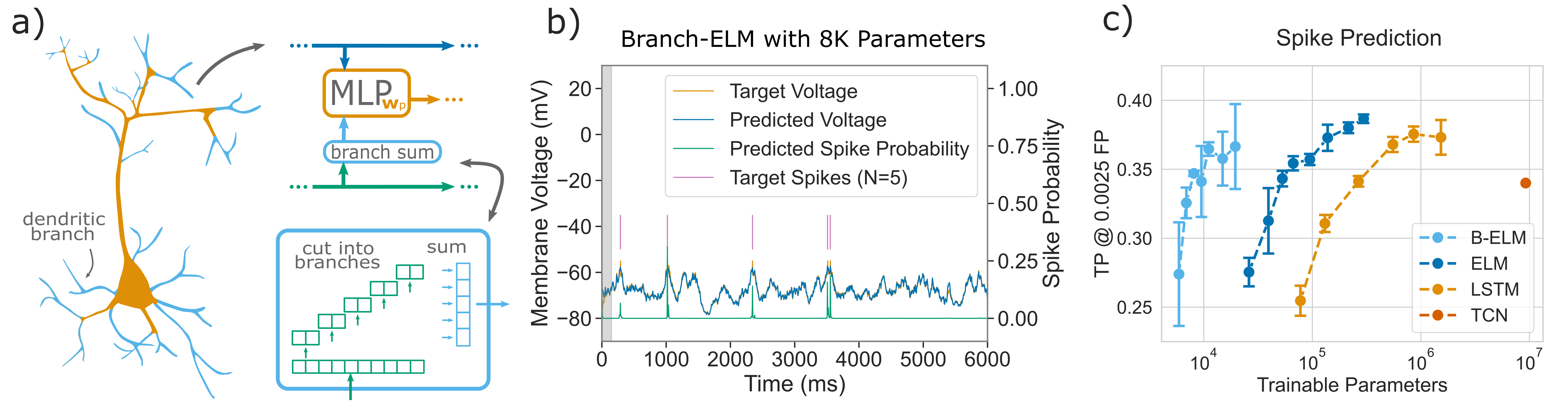
Figure 4: Coarse-grained modeling of synaptic integration significantly improves model efficiency. a) The integration mechanism dynamics of the ELM now computes the activity of individual dendritic branches as a simple sum of their respective synaptic inputs first before passing them on to the $\text{MLP}_{{\color[rgb]{0.87109375,0.5625,0.01953125}\bm{w_{p}}}}$, where $d_{\mathrm{tree}}$ is the number of branches and $d_{\mathrm{brch}}$ the number of synapses per branch. b) Accurate predictions using a Branch-ELM neuron with merely 8104 parameters (for zoomed in version with model dynamics see Fig. S7). c). The new Branch-ELM neuron improves on the ELM neuron by about 7$\times$ in terms of parameter efficacy (same ELM hyper-parameters). Differences in model quality are particularly obvious when examining True-Positive rate at a low False-Positive rate.

Surprisingly, even with this strong simplification, the Branch-ELM neuron model is able to retain its predictive performance while requiring a modest 8K trainable parameters to substantially cross the performance threshold. This corresponds to roughly 7$\times$ reduction over the vanilla ELM neuron. We also find that a combination of $d_{\mathrm{tree}}=35$ and $d_{\mathrm{brch}}=65$ still achieved over $0.991$ AUC with only 5479 trainable parameters, corroborating the assumption of the near-linear computation within dendritic branches and inviting future investigation of minimal required synaptic nonlinearity. However, this simplification ideally utilizes the knowledge of the exact morphology for modeling the neuron, or the relationship structure in the input data in case of other tasks; thus most consecutive experimental reports are for the vanilla ELM neuron.

4.2 Evaluating temporal processing capabilities on a bio-inspired task

The Spiking Heidelberg Digits (SHD) dataset comprises spike-encoded spoken digits (0-9) in German and English Cramer et al. (2020). The digits were encoded using 700 input channels in a biologically inspired artificial cochlea. Each channel represents a narrow frequency band with the firing rate coding for the signal power in this band, resulting in an encoding that resembles the spectrogram of the spoken digit (see Figure 5a).

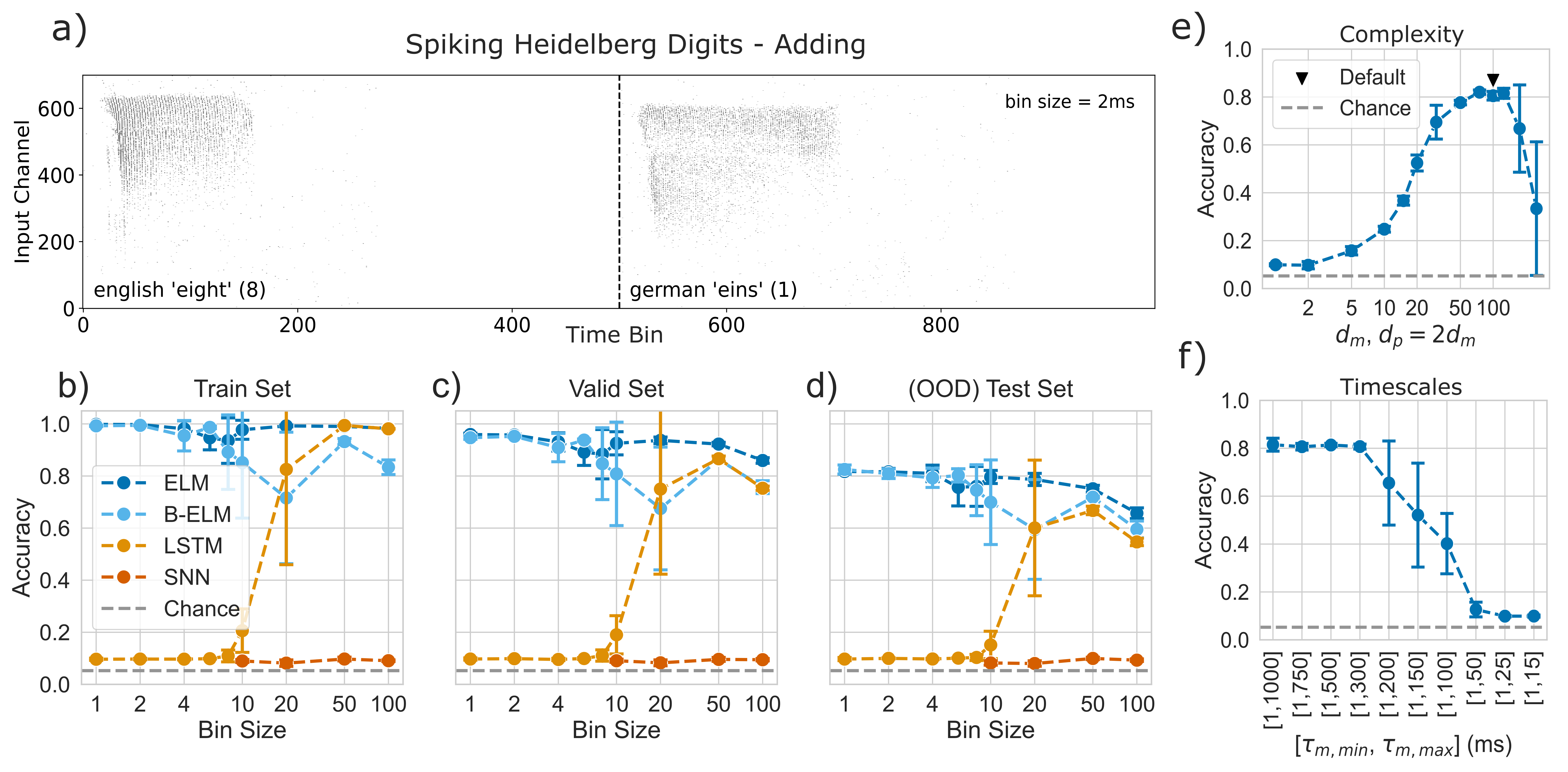
Figure 5: The ELM neuron performs well on long and sparse data using longer timescales. a) Sample from the biologically motivated SHD-Adding dataset (based on Cramer et al. (2020)), each dot is an input spike, and a vertical dashed line is a guide for the eye indicating the separation of the two digits (not communicated to the network). b-d) The ELM neuron (186K params.) consistently outperforms a classic LSTM (956K params.), especially for smaller bin sizes (meaning longer training samples), and LSTM-performance cannot be fully recovered even for larger bin sizes. The Branch-ELM (67K params.) can retain performance for fine-grained binning at a much reduced model size. Our Leaky Integrate and Fire (LIF) (51K params.) Spiking Neural Network (SNN) does not manage to achieve good performance for any bin size, and training becomes unstable for long sequences. e) and f) Ablations using bin size of 2ms with test set performance reported. e) Solving SHD-Adding requires ELM neuron to have a higher complexity than required for NeuronIO (large model unstable with $\lambda=5$). f) Longer memory timescales are crucial for extracting long-range dependencies.

Motivated by recent findings that most neuromorphic benchmark datasets only require minimal temporal processing abilities Yang et al. (2021), we introduce the SHD-Adding dataset by concatenating two uniformly and independently sampled SHD digits and setting the target to their sum (regardless of language) (see Figure 5a). Solving this dataset necessitates identifying each digit on a shorter timescale and computing their sum by integrating this information over a longer timescale, which in turn requires retaining the first digit in memory. Whether single cortical neurons can solve this exact task is unclear; however, it has been shown that even single neurons possibly encode and perform basic arithmetics in the medial temporal lobe Cantlon & Brannon (2007); Kutter et al. (2018; 2022).

The ELM neuron demonstrates its ability to solve the summing task across various temporal resolutions, as determined by the bin size. As we vary the bin size from 1ms (comprising 2000 bins in total, corresponding to the maximum temporal detail and longest required memory retention) to 100 (with 20 bins in total, corresponding to the minimum temporal detail and shortest memory retention), the ELM neuron’s performance remains robust, degrading only gracefully for greater bin sizes (see Figure 5b-d). Further, the performance is also maintained when testing on two held-out speakers, showing that the ELM neuron remains comparatively robust out-of-distribution. In contrast, the LSTM struggles with this task, especially when the bin size is below 50, due to memory issues. As the bin size increases, the LSTM’s performance does not improve because larger bin sizes leads to the loss of crucial temporal details. This outcome underlines the importance of a model’s ability to integrate complex synaptic information effectively (see Figure 5e), and the utility of longer neuron-internal timescales for learning long-range dependencies, potentially necessary for cortical neuron’s operation (see Figure 5f).

4.3 Evaluating on complex and very long temporal dependency tasks

To test the extent and limits of the ELM neuron’s ability to extract complex long-range dependencies, we use the classic Long Range Arena (LRA) benchmark datasets Tay et al. (2021). It consists of classification tasks; three image-derived datasets Image, Pathfinder, and Pathfinder-X (images being converted to a grayscale pixel sequence), and three text-based datasets ListOps, Text, and Retrieval. Pixel and token sequences were encoded categorically, however, only considering 8 or 16 different grayscale levels for images. In particular, the Pathfinder-X task is notoriously difficult, as the task is to determine whether two dots are connected by a path in a $128\times 128$ (~16k) image.

Table 1: Accuracy on Long Range Arena (LRA) Benchmark Tay et al. (2021).

	Image	Pathfinder	Pathfinder-X	ListOps	Text	Retrieval
ELM Neuron (ours)	49.62	71.15	77.29	46.77	80.3	84.93
Chr.-LSTM Tallec & Ollivier (2018)	46.09	70.79	FAIL∗	44.55	75.4	82.87
# parameters	~100k	~100k	~100k	~100k	~200k	~150k
Transformer Vaswani et al. (2017)	42.44	71.4	FAIL	36.37	64.27	57.46
Longformer Beltagy et al. (2020)	42.22	69.71	FAIL	35.63	62.85	56.89
S4 Gu et al. (2021)	87.26	86.05	88.1	58.35	76.02	87.09
Mega Ma et al. (2023)	90.44	96.01	97.98	63.14	90.43	91.25
# parameters	~600k	~600k	~600k	~600k	~600k	~600k

The ELM neuron can solve challenging long-range sequence modeling tasks. The mean accuracy and approximate model size are displayed. The ELM neuron routinely scores higher than the Chrono-LSTM or the much larger Transformer or Longformer, and only the large multi-layered architectures tuned specifically for these tasks, such as S4 or Mega, are able outperform it. Surprisingly, it is also the only non purpose built model that is able to reliably solve the notoriously challenging $16$K sample length Pathfinder-X task (albeit using much longer ${\color[rgb]{0.0078125,0.62109375,0.44921875}\bm{\tau_{s}}}$). Model sizes of the bottom baseline models extracted from Gu et al. (2021)Ma et al. (2023)Tay et al. (2021). Training details and model hyper-parameters detailed in Appendix section B, and Tables S2 and S3.

Our results are summarized in Table 1, where we compare the ELM neuron against several strong baselines. The model most comparable to ours is an LSTM with derived explicit gating bias initialization for effectively longer internal timescales Tallec & Ollivier (2018) (Chrono-LSTM). When comparing the two, we find that both models consistently perform well, except on the Pathfinder-X task which only the ELM is able to reliably solve, albeit using longer ${\color[rgb]{0.0078125,0.62109375,0.44921875}\bm{\tau_{s}}}$ than usual. The larger self-attention-based models trail further behind, with both Transformer Vaswani et al. (2017) and Longformer Beltagy et al. (2020) completely failing to solve the Pathfinder-X task Tay et al. (2021). Only the purpose built architectures such as S4 Gu et al. (2021) and Mega Ma et al. (2023) (current SOTA) perform better, but they require many layers of processing and many more parameters than an ELM neuron, with merely uses 150 memory units and typically ~100k parameters.

Overall, the results suggest that the simple ELM neuron architecture is capable of reliably solving challenging tasks with very long temporal dependencies. Crucially this required using memory timescales initialized according to the task length, and highly nonlinear synaptic integration into 150 memory units (See appendix B). While the LRA benchmark revealed the single ELM neurons limits, we hypothesize that assembling ELM neurons into layered networks might give it enough processing capabilities to catch up with the deep models, but leave this investigation to future work.

5 Discussion

In this study, we introduced a biologically inspired recurrent cell, the Expressive Leaky Memory (ELM) neuron, and demonstrated its capability to fit the full spike-level input/output mapping of a high-fidelity biophysical neuron model (NeuronIO). Unlike previous works that achieved this fit with millions of parameters, a variant of our model only requires a few thousand, thanks to the careful design of the architecture exploiting appropriate inductive biases. Furthermore, unlike existing neuron models, the ELM can effectively model neuron without making rigid assumptions about the number of memory states and their timescales, or the degree of nonlinearity in its synaptic integration.

We further scrutinized the implications and limitations of this design on various long-range dependency datasets, such as a biologically-motivated neuromorphic dataset (SHD-Adding), and some notoriously challenging ones from the machine learning literature (LRA). Leveraging slowly decaying memory units and highly nonlinear dendritic integration into multiple memory units, the ELM neuron was found to be quite competitive, in particular, compared to classic RNN architectures like the LSTM, a notable feat considering its much simpler architecture and biological inspiration.

It should be noted though, that in spite of its biological motivation, our model cannot give mechanistic explanations of neural computations as biophysical models do. Many biological implementation details are abstracted away in favor of computational efficiency and conceptual insight, and the required/recovered ELM neuron hyper-parameters are dependent on what constitutes a sufficiently good fit and the models subsequent use-case. Furthermore, ELM learning likely relies on neuronal plasticity beyond synapses, the extent of which in biological neurons is still a subject of debate. Additionally, our neuron model is missing some prominent macroscopic features like the distinction between apical/basal dendrites, and the modeling of dendrites is rudimentary and relies on oversampling synaptic inputs so far. Finally, given the use of BPTT for training, and the comparatively larger ELM neuron sizes on the later datasets, one should be careful to directly draw conclusions about the learning capabilities of individual biological cortical neurons.

Despite these caveats, the ELM’s ability to efficiently fit cortical neuron I/O and it’s promising performance on machine learning tasks suggests that we are beginning to incorporate the inductive biases that drive the development of more intelligent systems. Future research focused on connecting smaller ELM neurons into larger networks could provide even more insights into the necessary and dispensable elements for building smarter machines.

Acknowledgments

This work was supported by a Sofja Kovalevskaja Award from the Alexander von Humboldt Foundation. We acknowledge the support from the BMBF through the Tübingen AI Center (FKZ: 01IS18039A and 01IS18039B). AL, GM, and BS are members of the Machine Learning Cluster of Excellence, EXC number 2064/1 – Project number 39072764. Majority of computations were performed on the HPC system Raven at the Max Planck Computing and Data Facility.

Appendix

Appendix A Implementation Details

All computations were performed using Python 3.9, and the following libraries were instrumental in our implementation: jax 0.3.14 (coupled with jaxlib 0.3.10 as a GPU back-end) for auto-grad and auto-vectorization; equinox 0.8.0, a jax-based neural network library; optax 0.1.3, a jax-based optimizer library; and pytorch 1.12.1 for data-loading. The code used for our experiments will be accessible at the public repository upon publication.

Table S1: The default ELM neuron parameters and recommendations.

Hyper-Parameter	NeuronIO	Tuning Recommendation
$\bm{s_{0}}$	0	/
$\bm{w_{s}}$	0.5	/
$\bm{w_{s}}$ (bounds)	> 0	>= 0
$\bm{\tau_{s}}$	all 5ms	greater for long & sparse data
$\bm{m_{0}}$	0	/
$d_{m}$	$20$	up to $250$
$\bm{\tau_{m}}$ (init technique)	equally spaced	evenly spaced on log scale
$\bm{\tau_{m}}$ (init range)	1ms,100ms	1ms,data length
$\bm{\tau_{m}}$ (bounds)	0ms,500ms	same as for $\bm{\tau_{m}}$
$\text{MLP}_{w_{p}}$ (nonlineary)	ReLU	/
$\text{MLP}_{w_{p}}$ (bias)	True	/
$\text{MLP}_{w_{p}}$ (init technique)	Kaiming Uniform	/
$l_{\mathrm{mlp}}$	$1$	/
$d_{\mathrm{mlp}}$	$2*{\color[rgb]{0.00390625,0.44921875,0.69921875}d_{m}}$	$2*{\color[rgb]{0.00390625,0.44921875,0.69921875}d_{m}}$
$\lambda$	10	5
$\bm{w_{y}}$ (bias)	True	/
$\bm{w_{y}}$ (init technique)	Kaiming Uniform	/
$d_{\mathrm{tree}}$	45	get all input 2-5 times over
$d_{\mathrm{brch}}$	100	$2*{\color[rgb]{0.3359375,0.70703125,0.9140625}d_{\mathrm{tree}}}$

For all experiments $\bm{w_{y}}$, $w_{p}$ and $\bm{\tau_{m}}$ were learnable, with $\bm{w_{s}}$ crucially also learnable for Branch-ELM.

Recommended default and tuning parameters:

We primarily recommend ablating $d_{m}$. In case of small $d_{m}$, exploring larger relative $d_{\mathrm{mlp}}$ or larger $\lambda$ might yield improved performance. For a combination of large $d_{m}$ with large $\lambda$ we have observed increased traing instability. The timescales $\bm{\tau_{m}}$ should generally be derived from the dataset length and the suspected timescales of the temporal dependencies within the data. Increasing $\bm{\tau_{s}}$ may help to enhance learning speed in case of long and sparse data. When using the Branch-ELM it is important to sufficiently over-sample the input (more synapses than input) as we suspect significant expressivity stemming from $\bm{w_{s}}$ doing the selection. Additional recommendations are summarized in Table S1.

Timescale parametrization:

The memory timescales ${\color[rgb]{0.00390625,0.44921875,0.69921875}\bm{\tau_{m}}}$ are model parameters and directily learnable. They are constrained to an apriori-specified bound, which is enforced through a $sigmoid$ rectification (the lower bound being at least $0$). By defining ${\color[rgb]{0.00390625,0.44921875,0.69921875}\bm{\kappa_{m}}}=\exp(\nicefrac{{-\Delta t}}{{{\color[rgb]{0.00390625,0.44921875,0.69921875}\bm{\tau_{m}}}}})$, the resulting values are ensured to be within $[0,1]$ for all valid $\bm{\tau_{m}}$, irrespective of $\Delta t$. In preliminary experiments we observed increased training stability as opposed to directly learning ${\color[rgb]{0.00390625,0.44921875,0.69921875}\bm{\kappa_{m}}}$.

The $\lambda$ hyper-parameter:

We found that enabling greater changes in ${\color[rgb]{0.87109375,0.5625,0.01953125}\bm{\Delta m_{t}}}$ by introducing a multiplicative factor ${\color[rgb]{0.87109375,0.5625,0.01953125}\lambda}$ improved training performance. Interestingly, this parameter can be seen as effectively implementing a $\lambda$ times faster input-timescale (than the forget timescale ${\color[rgb]{0.00390625,0.44921875,0.69921875}\bm{\tau_{m}}}$). This notion can be explicitly implemented by calculating ${\color[rgb]{0.00390625,0.44921875,0.69921875}\bm{\kappa_{m^{\prime}}}}=\exp(\nicefrac{{-\Delta t{\color[rgb]{0.87109375,0.5625,0.01953125}\lambda}}}{{{\color[rgb]{0.00390625,0.44921875,0.69921875}\bm{\tau_{m}}}}})$. The substitution holds for ${\color[rgb]{0.00390625,0.44921875,0.69921875}\bm{\tau_{m}}}>>{\color[rgb]{0.87109375,0.5625,0.01953125}\lambda}>1$, and only diverges for small ${\color[rgb]{0.00390625,0.44921875,0.69921875}\bm{\tau_{m}}}$, where it allows for less stark ${\color[rgb]{0.00390625,0.44921875,0.69921875}\bm{m}}$ changes than the original implementation.

Appendix B Datasets and Training Details

General training setup:

For each task and dataset, the training dataset was deterministically split to create a consistent validation dataset, which was used for model selection during training and hyperparameter tuning. By default all models were trained using Backpropagation Through Time (BPTT) with a batch size of 8 and the Adam optimizer, employing a learning rate of $5e^{-4}$ and a cosine-decay schedule across the entire training duration. All experiments were run on a single A100-40GB or A100-80GB and ran less than 24h, Pathfinder-X being the notable exception.

NeuronIO Dataset:

For training and evaluation the dataset was pre-processed in accordance with Beniaguev et al. (2021), by capping somatic membrane voltage at -55mV and subtracting a bias of -67.7mV. Additionally, the somatic membrane voltage was scaled by 1/10 for training. Training samples were 500ms long with a 1ms bin size and $\Delta t$. The ELM neuron used the default parameters from Table S1. Models were trained for 30 epochs of 11,400 batches per epoch using Binary Cross Entropy (BCE) for spike prediction and Mean Squared Error (MSE) for somatic voltage prediction, with equal weighting. Loss was calculated after a 150ms burn-in period. The mean and standard deviation over three runs is reported, with Root Means Squared Error (RMSE) and Area Under the Receiver Operator Curve (AUC) for voltage and spike prediction, respectively.

Spiking Heidelberg Digits (Adding) Datasets:

The digits were preprocessed by cutting them to a uniform length of one second and binning the spikes using various bin sizes, the default being 10ms. The models were trained using the Adamax optimizer with a learning rate of $5e^{-3}$ for 70 epochs, for 814 and 2000 batches per epoch for SHD and SHD-Adding respectively, with $\Delta t$ set to the bin size, and dropout probability set to 0.5. The ELM used $\lambda=5$, $d_{m}=100$ and $\tau_{m}$ initialized evenly spaced between 1ms and 150ms with bounds of 0ms to 1000ms, and the LSTM used a hidden size of 250 and additional recurrent dropout of 0.3, while the SNN used a learning rate of $2e^{-3}$ no dropout but a $l1$ regularization on the spikes of $0.01$. Models were trained using the Cross-Entropy (CE) loss on the last float output of the respective model, and the performance was reported as prediction Accuracy, with mean and standard deviation calculated over five runs (chance performance being 1/19).

Long Sequence Modeling Datasets: The images-based datasets were preprocessed by binning the individual greyscale values (256 total) into 16, or 8 for Pathfinder-X, different levels. For the text based datasets a simple one-hot token encoding was used. For the Retrieval task with a two-tower setup, the latent-dimension was 75 for both models. The ELM neuron used a larning rate of $2e-4$ the LSTM model worked with $1e-3$ best. All trained using Cross-Entropy (CE) loss on the last output of the model, and the performance is reported as prediction Accuracy. The mean over three runs is reported for all experiments.

Table S2: The ELM neuron configuration

Dataset	Input Dim	Batch Size	Epochs	$\tau_{s}$	Timescales
Image	16	384	300	5	logspace: $1-10^{3}$
Pathfinder	16	384	300	5	logspace: $1-10^{3}$
Pathfinder-X	8	768	300	150	logspace: $1-2*10^{4}$
ListOps	25	384	150	5	logspace: $1-2*10^{3}$
Text	169	384	150	5	logspace: $1-4*10^{3}$
Retrieval	105	384	150	5	logspace: $1-4*10^{3}$

The ELM memory timescale bounds were matched to the initialization range. The ELM used a synapse tau of $150ms$ on the Pathfinder-X dataset, which we observed to increase the learning speed significantly, however, smaller synapse tau can also work. Otherwise the hyper-parameters were harmonized as much as possible, to demonstrate the robustness of the hyper-parameter choice.

Table S3: The Chrono-LSTM configuration

Dataset	Input Dim	Batch Size	Epochs	Timescales
Image	$16$	$384$	300	uniform: $1-2*10^{3}$
Pathfinder	$16$	$384$	300	uniform: $1-2*10^{3}$
Pathfinder-X	$8$	$768$	300	uniform: $1-2*10^{4}$
ListOps	$25$	$384$	150	uniform: $1-4*10^{3}$
Text	$169$	$384$	150	uniform: $1-8*10^{3}$
Retrieval	$105$	$384$	150	uniform: $1-8*10^{3}$

The Chrono-LSTM hyper-parameter tuning primarily concerned the learning rates and hidden sizes, however a learning rate of $1e^{-3}$ (among the tested) and a hidden size of $150$ (max tested) consistently performed best, the exception being Pathfinder-X, where during tuning a single run using a smaller hidden size performed slightly above change.

Appendix C Additional Results

We provide an evaluation of the classic Leaky Integrate and Fire (LIF) neuron model (with learnable membrane timescale and bias unit for linear integration), and an ELM neuron model with only a single memory unit (and timescale) with linear synaptic integration (additional parameters due to bias units, readout and other implementation details). The LIF’s internal membrane voltage was directly fit to the target voltage, and its output spike directly to the target spikes, using otherwise same training methodology as described in Section B.

Table S4: Evaluating Tiny Models on NeuronIO

Model	Soma RMSE	Spike AUC	# parameters
(classic) LIF	2.29	0.9117	1280
(simplest) ELM	1.60	0.9255	1286

While both models perform much worse than the reference performance threshold of $0.991AUC$, the ELM neuron performs slightly better in particular for somatic prediction. This could be the result of the ELM neuron, similarly to the underlying biophysical model, not enforcing an explicit hard memory reset after spiking. Additionally, the LIF’s shortcoming in capturing the I/O relationship accurately directly highlight the need for a more flexible phenomenological neuron model.

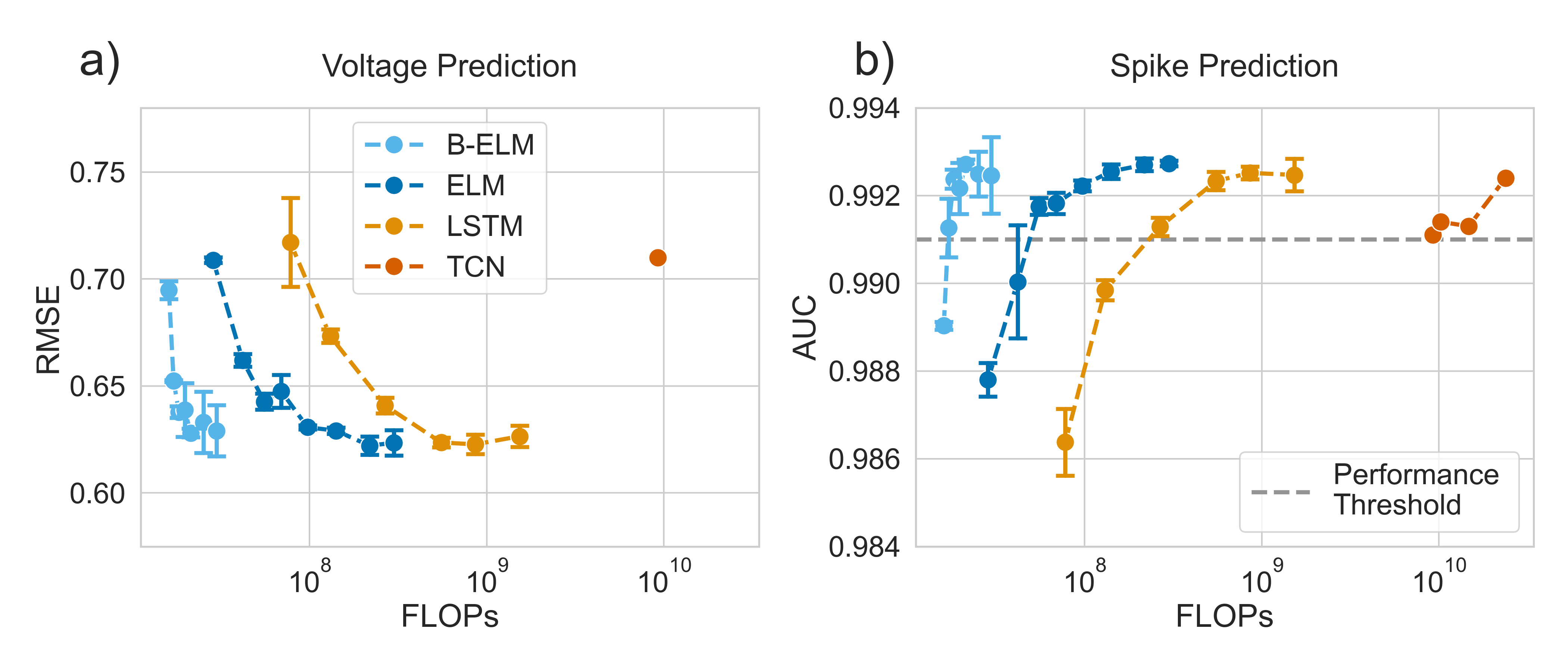
Figure S1: The ELM neuron is a computationally efficient model of cortical neuron. Similar figure to 2c and 2d, however, displaying FLOPs required to do inference on a single sample. a) and b) Voltage and spike prediction performance of the respective surrogate models. While previous works required around 10M parameters to make accurate spike predictions using a TCN Beniaguev et al. (2021), an LSTM baseline is able to do it with 266K, our ELM neuron model requires merely 53K, and our Branch-ELM neuron only a humble 8K, simultaneously achieving much better voltage prediction performance than the TCN. A throughput optimized ELM neuron implementation can potentially reduce the required FLOPs even further.

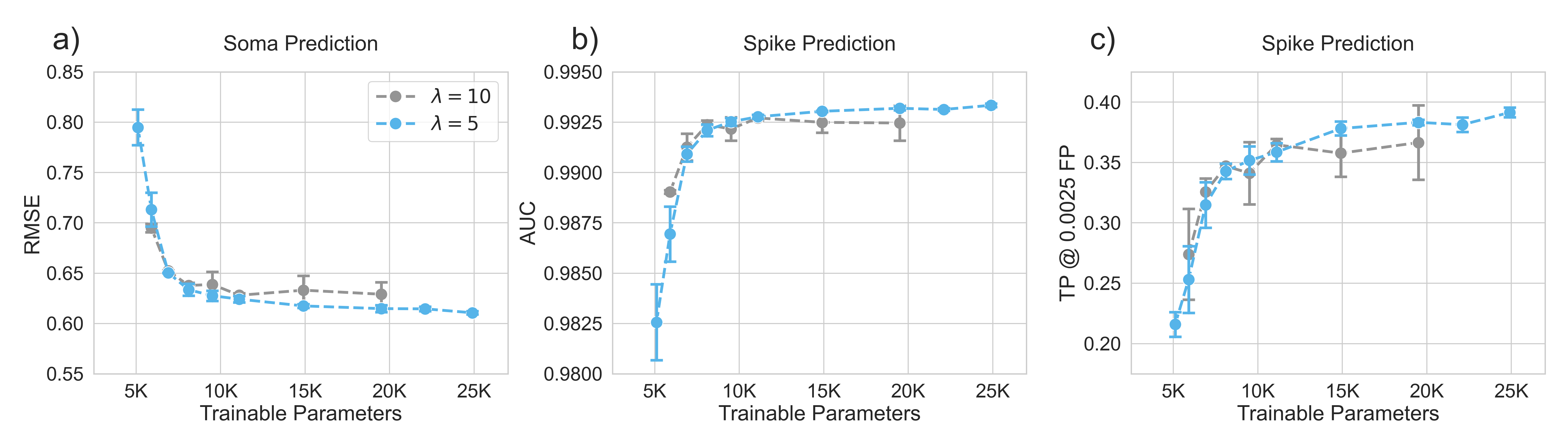
Figure S2: Branch-ELM neuron training is more stable with smaller $\lambda$. Evaluating a Branch-ELM with same hyper-parameters as in Figure 2, except with $\lambda=5$. Visibly, the variation in test set performance is reduced for most configurations, in particular for larger number of memory units, which results in new max performance for the model-type.

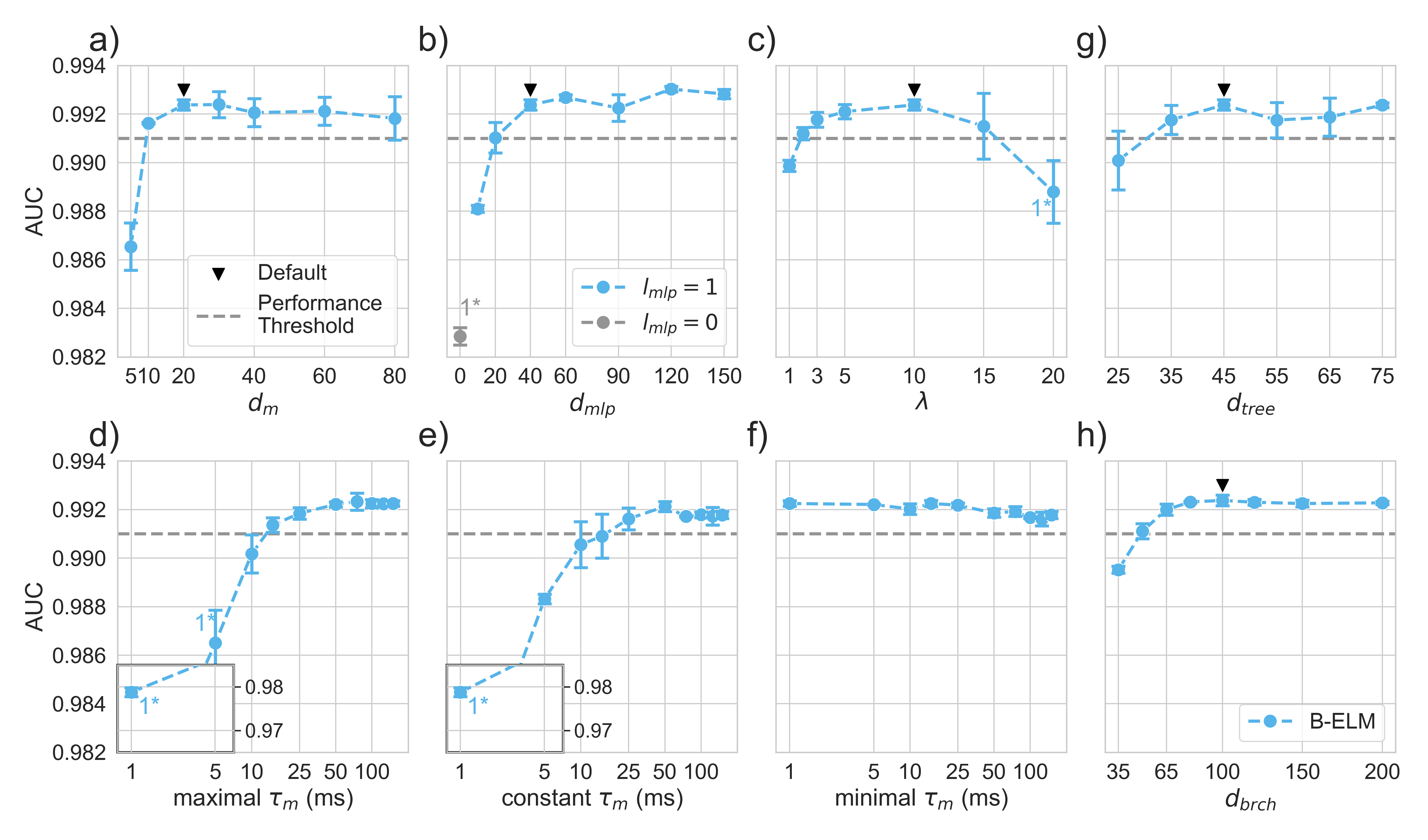
Figure S3: The ELM neuron gives relevant neuroscientific insights. Ablations on NeuronIO of different hyperparameters of an Branch-ELM neuron with AUC $\approx 0.992$, with default hyperparameters. The number of removed divergent runs marked with $1^{*}$. a) We find above memory-like hidden states to be required for accurate predictions, much more than typical phenomenological models use Izhikevich (2004); Dayan & Abbott (2005). b) Highly nonlinear integration of synaptic input is required, in line with recent neuroscientific findings Stuart & Spruston (2015); Jones & Kording (2022); Larkum (2022). c) Allowing greater updates to the memory units is beneficial, however, too large ones increase training instability. d-f) Ablations of memory timescale (initialization and bounding) range or (constant) value, with the default range being 1ms-150ms. Timescales around 25ms-50ms seem to be the most useful (matching the typical membrane timescale in the cortex Dayan & Abbott (2005)); however, a lack can be partially compensated by longer timescales, even better than by the vanilla ELM. g) and h) Ablating the number of branches $d_{\mathrm{tree}}$ and number of synapses per branch $d_{\mathrm{brch}}$.

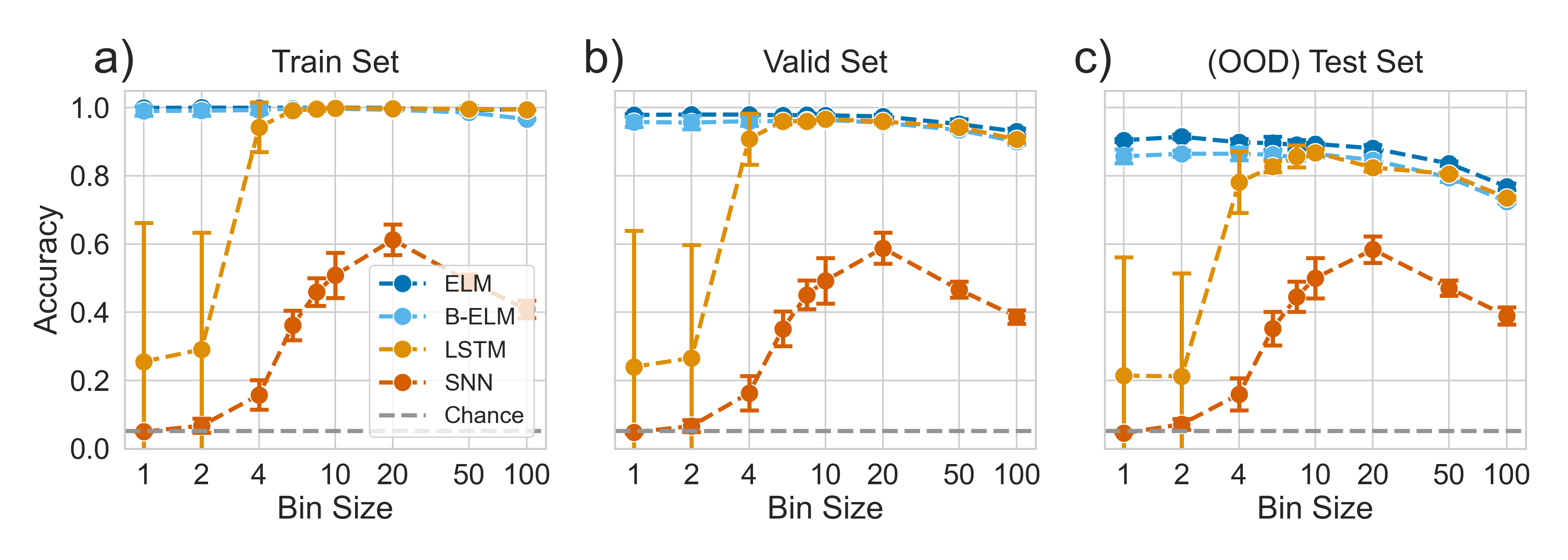
Figure S4: The ELM neuron performs well on typical spiking datasets. The following results are on the original Spiking Heidelberg Digits dataset Cramer et al. (2020). a-c) The ELM and Branch-ELM neuron reliably outperforms a classic LSTM, especially for smaller bin sizes (meaning longer training samples), and LSTM-performance cannot be fully recovered even for larger bin sizes. Our Leaky Integrate and Fire (LIF) Spiking Neural Network (SNN), however, does manage to achieve decent performance for intermediate bin sizes around 20, in contrast to the SHD-Adding dataset (see Figure 5).

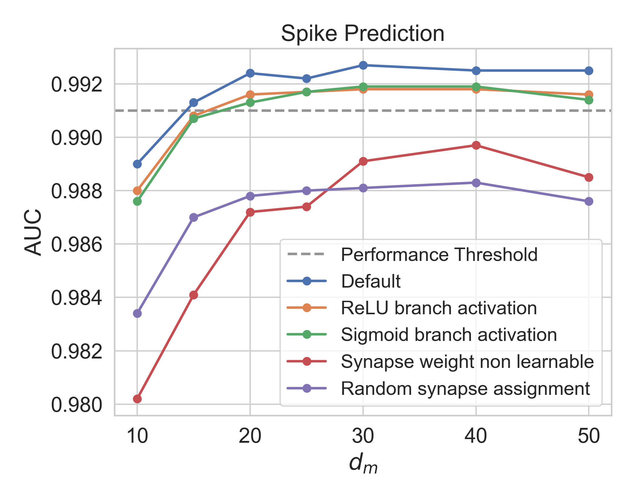
Figure S5: Ablating the ELM branch architecture on NeuronIO. Average test AUC displayed, using otherwise same hyper-parameters and training setup as in experiments in Figure 2. Exploiting the ordering in the synaptic input, and having learnable synapses is crucial for the Branch-ELM neuron model. Applying a specific nonlinearity on branch output slightly degrades performance.

Figure S6: Ablating the $\tau_{s}$ parameter on Pathfinder-X. Average and max test Accuracy displayed, using otherwise same hyper-parameters and training setup as in experiments in Table S2. While reliably achieving high performance requires larger $\tau_{s}$, smaller timescales can achieve even higher performance, although less reliably and take longer to pick up on learning signal.

Appendix D Additional Visualizations

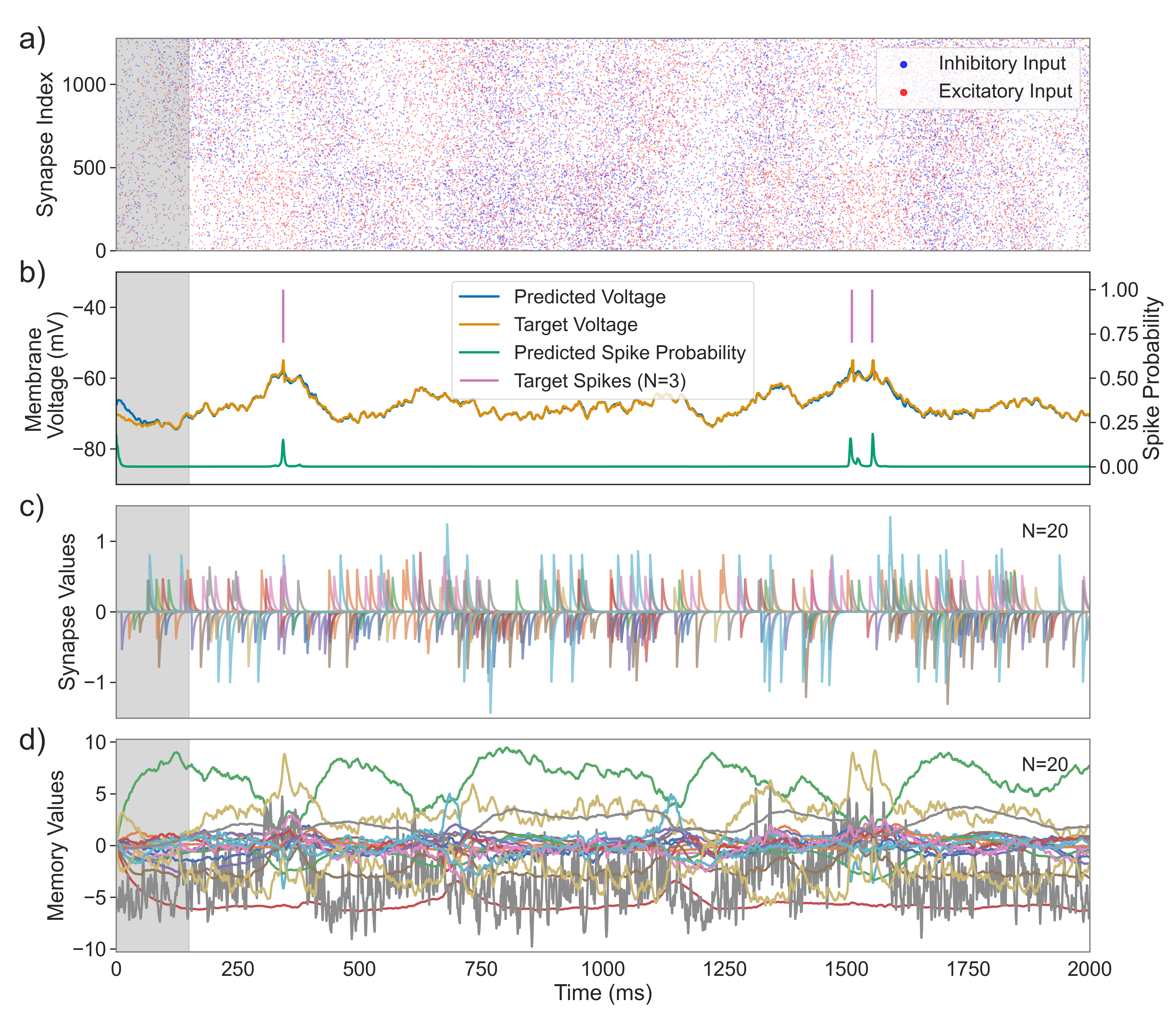
Figure S7: Visualization of ELM neuron dynamics. Extended visualization of Figure 2b for an ELM neuron achieving around 0.992 AUC. a) The synaptic input as the neuron model receives it, with excitatory input ($+1$) marked in red, and inhibitory input ($-1$) marked in blue. b) The ELM neurons predictions and the ground-truth targets for a regular sample from the data. Interestingly, the whole two seconds were inferred in one go (similar to Figure 4b), which shows its generalization capabilities beyond the training horizon of 500ms. c) A random subset of 20 synapses are visualized. Synapses receiving negative input will be deflected downwards. d) All 20 memory values are visualized. Some fluctuate more rapidly than others, typically proportional to their memory timescales.

Appendix E Reduced Implementation In Pytorch

⬇

import math

import torch

import torch.nn as nn

# NOTE: the 1e-6 used throughout are to avoid numerical instabilities

# NOTE: the tau_m bounds are enforced using a scaled sigmoid

# NOTE: the w_s bounds are enforced using relu (originally exp)

def scaled_sigmoid(x, lower_bound, upper_bound):

return (upper_bound - lower_bound) * torch.sigmoid(x) + lower_bound

def inverse_scaled_sigmoid(x, lower_bound, upper_bound):

x = torch.clamp(x, lower_bound + 1e-6, upper_bound - 1e-6)

return torch.log((x - lower_bound) / (upper_bound - x))

def custom_tanh(x):

return torch.tanh(x * 2 / 3) * 1.7159

class MLP(nn.Module):

"""Multi-layer␣perceptron␣(MLP)␣model."""

def __init__(self, input_size, hidden_size, num_output, num_layers):

super(MLP, self).__init__()

next_input_size = input_size

layers = []

for i in range(num_layers):

layers.append(nn.Linear(next_input_size, hidden_size))

layers.append(nn.ReLU())

next_input_size = hidden_size

layers.append(nn.Linear(next_input_size, num_output))

self.network = nn.Sequential(*layers)

def forward(self, x):

return self.network(x)

class ELM(nn.Module):

"""Expressive␣Leaky␣Memory␣(ELM)␣neuron␣model."""

def __init__(self, num_synapse, num_output, num_memory=100,

mlp_num_layers=1, memory_tau_min=10, memory_tau_max=1000,

lambda_value=3.0, tau_s_value=5.0, w_s_value=0.5, delta_t=1.0,

learn_memory_tau=False,mlp_hidden_size=None,use_num_branch=None):

super(ELM, self).__init__()

self.delta_t = delta_t

self.lambda_value = lambda_value

self.learn_memory_tau = learn_memory_tau

self.memory_tau_min = memory_tau_min

self.memory_tau_max = memory_tau_max

# configuration in case of using branches

self.use_num_branch = use_num_branch

if use_num_branch is not None:

assert num_synapse % use_num_branch == 0, "must␣be␣exactly␣divisible"

num_mlp_input = use_num_branch + num_memory

else:

num_mlp_input = num_synapse + num_memory

# initialization of model parameters

mlp_hidden_size = mlp_hidden_size if mlp_hidden_size else 2 * num_memory

self.mlp = MLP(num_mlp_input, mlp_hidden_size, num_memory, mlp_num_layers)

self.w_s = nn.parameter.Parameter(torch.full((num_synapse,), w_s_value))

self.w_y = nn.Linear(num_memory, num_output)

# initialization of time constants and decay factors

self.tau_s = torch.full((num_synapse,), tau_s_value)

self.kappa_s = torch.exp(-delta_t / torch.clamp(self.tau_s, min=1e-6))

self._proto_tau_m = torch.logspace(

math.log10(memory_tau_min + 1e-6),

math.log10(memory_tau_max - 1e-6),

num_memory,

)

self._proto_kappa_m = torch.exp(

-delta_t / torch.clamp(self._proto_tau_m, min=1e-6)

)

# configuration in case memory tau is learnable

if self.learn_memory_tau:

self._proto_tau_m = inverse_scaled_sigmoid(

self._proto_tau_m, memory_tau_min, memory_tau_max

)

self._proto_tau_m = nn.parameter.Parameter(self._proto_tau_m)

@property

def tau_m(self):

# ensure that tau_m is always up to date

if self.learn_memory_tau:

return scaled_sigmoid(

self._proto_tau_m, self.memory_tau_min, self.memory_tau_max

)

else:

return self._proto_tau_m

@property

def kappa_m(self):

# ensure that kappa_m is always up to date

if self.learn_memory_tau:

return torch.exp(-self.delta_t / torch.clamp(self.tau_m, min=1e-6))

else:

return self._proto_kappa_m

def dynamics(self, x, s_prev, m_prev, kappa_m):

# compute the dynamics for a single timestep

batch_size = x.shape[0]

s_t = self.kappa_s * s_prev + torch.relu(self.w_s) * x

if self.use_num_branch is not None:

syn_input = s_t.view(batch_size, self.use_num_branch, -1).sum(dim=-1)

else:

syn_input = s_t

delta_m_t = custom_tanh(

self.mlp(torch.cat([syn_input, kappa_m * m_prev], dim=-1))

)

m_t = kappa_m * m_prev + self.lambda_value * (1 - kappa_m) * delta_m_t

y_t = self.w_y(m_t)

return y_t, s_t, m_t

def forward(self, X):

# compute the the recurrent dynamics for a sample

batch_size, T, num_synapse = X.shape

kappa_m = self.kappa_m

s_prev = torch.zeros(batch_size, len(self.tau_s), device=X.device)

m_prev = torch.zeros(batch_size, len(self.tau_m), device=X.device)

outputs = []

for t in range(T):

y_t, s_prev, m_prev = self.dynamics(X[:, t], s_prev, m_prev, kappa_m)

outputs.append(y_t)

return torch.stack(outputs, dim=-2)

Appendix F Results in Table Format

Table S5: The Branch-ELM on NeuronIO

	Trainable Parameters	FLOPs	Voltage Prediction RMSE	Spike Prediction AUC
Memory Units
10	5.9K	16.04M	0.695 ± 0.004	0.989 ± 0.0001
15	6.9K	17.06M	0.652 ± 0.0	0.9913 ± 0.0007
20	8.1K	18.27M	0.638 ± 0.003	0.9924 ± 0.0002
25	9.5K	19.69M	0.639 ± 0.013	0.9922 ± 0.0006
30	11.1K	21.3M	0.628 ± 0.002	0.9927 ± 0.0001
40	14.9K	25.13M	0.633 ± 0.014	0.9925 ± 0.0005
50	19.5K	29.76M	0.629 ± 0.012	0.9925 ± 0.0009

Table S6: The ELM on NeuronIO

	Trainable Parameters	FLOPs	Voltage Prediction RMSE	Spike Prediction AUC
Memory Units
10	26.06K	28.49M	0.709 ± 0.001	0.9878 ± 0.0004
15	39.39K	41.84M	0.662 ± 0.003	0.99 ± 0.0013
20	52.92K	55.38M	0.643 ± 0.004	0.9918 ± 0.0002
25	66.65K	69.13M	0.648 ± 0.008	0.9918 ± 0.0002
35	94.71K	97.22M	0.631 ± 0.001	0.9922 ± 0.0001
50	138.3K	140.85M	0.629 ± 0.002	0.9925 ± 0.0002
75	214.95K	217.58M	0.622 ± 0.004	0.9927 ± 0.0001
100	296.6K	299.3M	0.623 ± 0.006	0.9927 ± 0.0001

Table S7: The LSTM on NeuronIO

	Trainable Parameters	FLOPs	Voltage Prediction RMSE	Spike Prediction AUC
Hidden Size
15	77.67K	77.77M	0.717 ± 0.021	0.9864 ± 0.0008
25	130.45K	130.61M	0.673 ± 0.003	0.9898 ± 0.0002
50	265.9K	266.23M	0.641 ± 0.004	0.9913 ± 0.0002
100	551.8K	552.45M	0.624 ± 0.002	0.9923 ± 0.0002
150	857.7K	858.68M	0.623 ± 0.005	0.9925 ± 0.0001
250	1529.5K	1531.13M	0.626 ± 0.005	0.9925 ± 0.0004

Table S8: SHD Results

		Train Accuracy	Valid Accuracy	Test Accuracy
Model	Bin Size
B-ELM	1	0.99 ± 0.01	0.96 ± 0.01	0.86 ± 0.02
	2	0.99 ± 0.01	0.96 ± 0.02	0.86 ± 0.01
	4	0.99 ± 0.01	0.96 ± 0.01	0.86 ± 0.02
	6	1.0 ± 0.0	0.96 ± 0.0	0.86 ± 0.01
	8	1.0 ± 0.0	0.96 ± 0.0	0.85 ± 0.01
	10	1.0 ± 0.0	0.96 ± 0.0	0.86 ± 0.01
	20	0.99 ± 0.0	0.96 ± 0.01	0.85 ± 0.01
	50	0.99 ± 0.0	0.93 ± 0.0	0.79 ± 0.01
	100	0.97 ± 0.0	0.9 ± 0.01	0.72 ± 0.01
ELM	1	1.0 ± 0.0	0.98 ± 0.0	0.9 ± 0.0
	2	1.0 ± 0.0	0.98 ± 0.0	0.91 ± 0.01
	4	1.0 ± 0.0	0.98 ± 0.0	0.9 ± 0.01
	6	1.0 ± 0.0	0.98 ± 0.0	0.9 ± 0.02
	8	1.0 ± 0.0	0.98 ± 0.0	0.89 ± 0.01
	10	1.0 ± 0.0	0.98 ± 0.0	0.89 ± 0.0
	20	1.0 ± 0.0	0.97 ± 0.0	0.88 ± 0.01
	50	0.99 ± 0.01	0.95 ± 0.01	0.84 ± 0.01
	100	1.0 ± 0.0	0.93 ± 0.01	0.77 ± 0.01
LSTM	1	0.26 ± 0.41	0.24 ± 0.4	0.21 ± 0.35
	2	0.29 ± 0.34	0.27 ± 0.33	0.21 ± 0.3
	4	0.94 ± 0.07	0.91 ± 0.07	0.78 ± 0.09
	6	0.99 ± 0.0	0.96 ± 0.01	0.83 ± 0.02
	8	1.0 ± 0.0	0.96 ± 0.0	0.86 ± 0.03
	10	1.0 ± 0.0	0.97 ± 0.0	0.87 ± 0.01
	20	1.0 ± 0.0	0.96 ± 0.0	0.82 ± 0.01
	50	1.0 ± 0.0	0.94 ± 0.01	0.81 ± 0.0
	100	0.99 ± 0.0	0.91 ± 0.01	0.74 ± 0.0
SNN	1	0.05 ± 0.0	0.05 ± 0.0	0.05 ± 0.0
	2	0.07 ± 0.02	0.07 ± 0.02	0.07 ± 0.02
	4	0.16 ± 0.04	0.16 ± 0.05	0.16 ± 0.05
	6	0.36 ± 0.04	0.35 ± 0.05	0.35 ± 0.05
	8	0.46 ± 0.04	0.45 ± 0.04	0.45 ± 0.04
	10	0.51 ± 0.07	0.49 ± 0.07	0.5 ± 0.06
	20	0.61 ± 0.04	0.59 ± 0.05	0.58 ± 0.04
	50	0.49 ± 0.02	0.47 ± 0.02	0.47 ± 0.02
	100	0.41 ± 0.03	0.39 ± 0.02	0.39 ± 0.03

Table S9: SHD-Adding Results

		Train Accuracy	Valid Accuracy	Test Accuracy
Model	Bin Size
B-ELM	1	0.99 ± 0.0	0.95 ± 0.01	0.83 ± 0.02
	2	0.99 ± 0.0	0.95 ± 0.0	0.81 ± 0.02
	4	0.95 ± 0.06	0.91 ± 0.05	0.79 ± 0.04
	6	0.99 ± 0.0	0.94 ± 0.0	0.8 ± 0.03
	8	0.89 ± 0.14	0.85 ± 0.14	0.75 ± 0.1
	10	0.85 ± 0.21	0.81 ± 0.2	0.7 ± 0.16
	20	0.72 ± 0.25	0.68 ± 0.24	0.59 ± 0.19
	50	0.93 ± 0.01	0.86 ± 0.01	0.72 ± 0.0
	100	0.83 ± 0.03	0.76 ± 0.02	0.59 ± 0.03
ELM	1	1.0 ± 0.0	0.96 ± 0.01	0.82 ± 0.01
	2	1.0 ± 0.0	0.96 ± 0.0	0.82 ± 0.01
	4	0.98 ± 0.03	0.93 ± 0.03	0.81 ± 0.03
	6	0.95 ± 0.05	0.89 ± 0.05	0.76 ± 0.07
	8	0.94 ± 0.09	0.88 ± 0.09	0.76 ± 0.08
	10	0.98 ± 0.04	0.93 ± 0.04	0.8 ± 0.03
	20	0.99 ± 0.0	0.94 ± 0.01	0.79 ± 0.02
	50	0.99 ± 0.0	0.92 ± 0.01	0.75 ± 0.01
	100	0.98 ± 0.0	0.86 ± 0.01	0.66 ± 0.02
LSTM	1	0.1 ± 0.0	0.1 ± 0.0	0.1 ± 0.01
	2	0.1 ± 0.0	0.1 ± 0.0	0.1 ± 0.0
	4	0.1 ± 0.0	0.1 ± 0.0	0.1 ± 0.0
	6	0.1 ± 0.0	0.1 ± 0.0	0.1 ± 0.0
	8	0.11 ± 0.02	0.11 ± 0.02	0.1 ± 0.01
	10	0.21 ± 0.08	0.19 ± 0.07	0.15 ± 0.05
	20	0.83 ± 0.37	0.75 ± 0.33	0.6 ± 0.26
	50	0.99 ± 0.0	0.87 ± 0.01	0.67 ± 0.02
	100	0.98 ± 0.0	0.75 ± 0.01	0.55 ± 0.01
SNN	10	0.09 ± 0.01	0.09 ± 0.01	0.08 ± 0.01
	20	0.08 ± 0.01	0.08 ± 0.01	0.08 ± 0.01
	50	0.1 ± 0.01	0.1 ± 0.01	0.1 ± 0.0
	100	0.09 ± 0.0	0.09 ± 0.0	0.09 ± 0.0

References

- Abraham et al. (2019) Wickliffe C Abraham, Owen D Jones, and David L Glanzman. Is plasticity of synapses the mechanism of long-term memory storage? NPJ science of learning, 4(1):9, 2019.
- Almog & Korngreen (2016) Mara Almog and Alon Korngreen. Is realistic neuronal modeling realistic? Journal of neurophysiology, 116(5):2180–2209, 2016.
- Aru et al. (2020) Jaan Aru, Mototaka Suzuki, and Matthew E Larkum. Cellular mechanisms of conscious processing. Trends in Cognitive Sciences, 24(10):814–825, 2020.
- Bellec et al. (2020) Guillaume Bellec, Franz Scherr, Anand Subramoney, Elias Hajek, Darjan Salaj, Robert Legenstein, and Wolfgang Maass. A solution to the learning dilemma for recurrent networks of spiking neurons. Nature Communications, 11(1):3625, December 2020. ISSN 2041-1723. doi: 10.1038/s41467-020-17236-y. URL http://www.nature.com/articles/s41467-020-17236-y.
- Beltagy et al. (2020) Iz Beltagy, Matthew E Peters, and Arman Cohan. Longformer: The long-document transformer. arXiv preprint arXiv:2004.05150, 2020.
- Beniaguev et al. (2021) David Beniaguev, Idan Segev, and Michael London. Single cortical neurons as deep artificial neural networks. Neuron, 109(17):2727–2739, 2021.
- Bicknell & Häusser (2021) Brendan A Bicknell and Michael Häusser. A synaptic learning rule for exploiting nonlinear dendritic computation. Neuron, 109(24):4001–4017, 2021.
- Brette & Gerstner (2005) Romain Brette and Wulfram Gerstner. Adaptive exponential integrate-and-fire model as an effective description of neuronal activity. Journal of neurophysiology, 94(5):3637–3642, 2005.
- Cantlon & Brannon (2007) Jessica F Cantlon and Elizabeth M Brannon. Basic Math in Monkeys and College Students. PLoS Biology, 5(12):e328, December 2007. ISSN 1545-7885. doi: 10.1371/journal.pbio.0050328. URL https://dx.plos.org/10.1371/journal.pbio.0050328.
- Cavanagh et al. (2020) Sean E Cavanagh, Laurence T Hunt, and Steven W Kennerley. A diversity of intrinsic timescales underlie neural computations. Frontiers in Neural Circuits, 14:615626, 2020.
- Chavlis & Poirazi (2021) Spyridon Chavlis and Panayiota Poirazi. Drawing inspiration from biological dendrites to empower artificial neural networks. Current opinion in neurobiology, 70:1–10, 2021.
- Cho et al. (2014) Kyunghyun Cho, Bart Van Merriënboer, Caglar Gulcehre, Dzmitry Bahdanau, Fethi Bougares, Holger Schwenk, and Yoshua Bengio. Learning phrase representations using rnn encoder-decoder for statistical machine translation. arXiv preprint arXiv:1406.1078, 2014.
- Cramer et al. (2020) Benjamin Cramer, Yannik Stradmann, Johannes Schemmel, and Friedemann Zenke. The heidelberg spiking data sets for the systematic evaluation of spiking neural networks. IEEE Transactions on Neural Networks and Learning Systems, 2020.
- Dayan & Abbott (2005) Peter Dayan and Laurence F Abbott. Theoretical neuroscience: computational and mathematical modeling of neural systems. MIT press, 2005.
- Gasparini & Magee (2006) Sonia Gasparini and Jeffrey C Magee. State-dependent dendritic computation in hippocampal ca1 pyramidal neurons. Journal of Neuroscience, 26(7):2088–2100, 2006.
- Gerstner & Kistler (2002) Wulfram Gerstner and Werner M Kistler. Spiking neuron models: Single neurons, populations, plasticity. Cambridge university press, 2002.
- Gerstner et al. (2014) Wulfram Gerstner, Werner M Kistler, Richard Naud, and Liam Paninski. Neuronal dynamics: From single neurons to networks and models of cognition. Cambridge University Press, 2014.
- Gidon et al. (2020) Albert Gidon, Timothy Adam Zolnik, Pawel Fidzinski, Felix Bolduan, Athanasia Papoutsi, Panayiota Poirazi, Martin Holtkamp, Imre Vida, and Matthew Evan Larkum. Dendritic action potentials and computation in human layer 2/3 cortical neurons. Science, 367(6473):83–87, 2020.
- Gjorgjieva et al. (2016) Julijana Gjorgjieva, Guillaume Drion, and Eve Marder. Computational implications of biophysical diversity and multiple timescales in neurons and synapses for circuit performance. Current opinion in neurobiology, 37:44–52, 2016.
- Grüning & Bohte (2014) André Grüning and Sander M Bohte. Spiking neural networks: Principles and challenges. In ESANN. Bruges, 2014.
- Gu et al. (2021) Albert Gu, Karan Goel, and Christopher Re. Efficiently modeling long sequences with structured state spaces. In International Conference on Learning Representations, 2021.
- Gütig & Sompolinsky (2006) Robert Gütig and Haim Sompolinsky. The tempotron: a neuron that learns spike timing–based decisions. Nature neuroscience, 9(3):420–428, 2006.
- Hawkins & Ahmad (2016) Jeff Hawkins and Subutai Ahmad. Why neurons have thousands of synapses, a theory of sequence memory in neocortex. Frontiers in neural circuits, pp. 23, 2016.
- Hay et al. (2011) Etay Hay, Sean Hill, Felix Schürmann, Henry Markram, and Idan Segev. Models of neocortical layer 5b pyramidal cells capturing a wide range of dendritic and perisomatic active properties. PLoS computational biology, 7(7):e1002107, 2011.
- Herz et al. (2006) Andreas VM Herz, Tim Gollisch, Christian K Machens, and Dieter Jaeger. Modeling single-neuron dynamics and computations: a balance of detail and abstraction. science, 314(5796):80–85, 2006.
- Hochreiter & Schmidhuber (1997) Sepp Hochreiter and Jürgen Schmidhuber. Long short-term memory. Neural computation, 9(8):1735–1780, 1997.
- Hodassman et al. (2022) Shiri Hodassman, Roni Vardi, Yael Tugendhaft, Amir Goldental, and Ido Kanter. Efficient dendritic learning as an alternative to synaptic plasticity hypothesis. Scientific Reports, 12(1):6571, 2022.
- Hodgkin & Huxley (1952) Alan L Hodgkin and Andrew F Huxley. A quantitative description of membrane current and its application to conduction and excitation in nerve. The Journal of physiology, 117(4):500, 1952.
- Holtmaat et al. (2009) Anthony Holtmaat, Tobias Bonhoeffer, David K Chow, Jyoti Chuckowree, Vincenzo De Paola, Sonja B Hofer, Mark Hübener, Tara Keck, Graham Knott, Wei-Chung A Lee, et al. Long-term, high-resolution imaging in the mouse neocortex through a chronic cranial window. Nature protocols, 4(8):1128–1144, 2009.
- Izhikevich (2004) Eugene M Izhikevich. Which model to use for cortical spiking neurons? IEEE transactions on neural networks, 15(5):1063–1070, 2004.
- Jadi et al. (2014) Monika P Jadi, Bardia F Behabadi, Alon Poleg-Polsky, Jackie Schiller, and Bartlett W Mel. An augmented two-layer model captures nonlinear analog spatial integration effects in pyramidal neuron dendrites. Proceedings of the IEEE, 102(5):782–798, 2014.
- Jaeger (2002) Herbert Jaeger. Tutorial on training recurrent neural networks, covering bppt, rtrl, ekf and the" echo state network" approach. ., 2002.
- Jolivet et al. (2008) Renaud Jolivet, Felix Schürmann, Thomas K Berger, Richard Naud, Wulfram Gerstner, and Arnd Roth. The quantitative single-neuron modeling competition. Biological cybernetics, 99(4):417–426, 2008.
- Jones & Kording (2021) Ilenna Simone Jones and Konrad Paul Kording. Might a single neuron solve interesting machine learning problems through successive computations on its dendritic tree? Neural Computation, 33(6):1554–1571, 2021.
- Jones & Kording (2022) Ilenna Simone Jones and Konrad Paul Kording. Do biological constraints impair dendritic computation? Neuroscience, 489:262–274, 2022.
- Kandel et al. (2000) Eric R Kandel, James H Schwartz, Thomas M Jessell, Steven Siegelbaum, A James Hudspeth, Sarah Mack, et al. Principles of neural science, volume 4. McGraw-hill New York, 2000.
- Kobayashi et al. (2009) Ryota Kobayashi, Yasuhiro Tsubo, and Shigeru Shinomoto. Made-to-order spiking neuron model equipped with a multi-timescale adaptive threshold. Frontiers in computational neuroscience, pp. 9, 2009.
- Koch (1997) Christof Koch. Computation and the single neuron. Nature, 385(6613):207–210, 1997.
- Koch & Segev (2000) Christof Koch and Idan Segev. The role of single neurons in information processing. Nature neuroscience, 3(11):1171–1177, 2000.
- König et al. (1996) Peter König, Andreas K Engel, and Wolf Singer. Integrator or coincidence detector? the role of the cortical neuron revisited. Trends in neurosciences, 19(4):130–137, 1996.
- Kusupati et al. (2018) Aditya Kusupati, Manish Singh, Kush Bhatia, Ashish Kumar, Prateek Jain, and Manik Varma. Fastgrnn: A fast, accurate, stable and tiny kilobyte sized gated recurrent neural network. Advances in neural information processing systems, 31, 2018.
- Kutter et al. (2018) Esther F. Kutter, Jan Bostroem, Christian E. Elger, Florian Mormann, and Andreas Nieder. Single Neurons in the Human Brain Encode Numbers. Neuron, 100(3):753–761.e4, November 2018. ISSN 08966273. doi: 10.1016/j.neuron.2018.08.036. URL https://linkinghub.elsevier.com/retrieve/pii/S0896627318307414.
- Kutter et al. (2022) Esther F. Kutter, Jan Boström, Christian E. Elger, Andreas Nieder, and Florian Mormann. Neuronal codes for arithmetic rule processing in the human brain. Current Biology, 32(6):1275–1284.e4, March 2022. ISSN 09609822. doi: 10.1016/j.cub.2022.01.054. URL https://linkinghub.elsevier.com/retrieve/pii/S0960982222001166.
- Lafourcade et al. (2022) Mathieu Lafourcade, Marie-Sophie H van der Goes, Dimitra Vardalaki, Norma J Brown, Jakob Voigts, Dae Hee Yun, Minyoung E Kim, Taeyun Ku, and Mark T Harnett. Differential dendritic integration of long-range inputs in association cortex via subcellular changes in synaptic ampa-to-nmda receptor ratio. Neuron, 2022.
- Larkum (2022) Matthew Larkum. Are dendrites conceptually useful? Neuroscience, 2022.
- Losonczy et al. (2008) Attila Losonczy, Judit K Makara, and Jeffrey C Magee. Compartmentalized dendritic plasticity and input feature storage in neurons. Nature, 452(7186):436–441, 2008.
- Ma et al. (2023) Xuezhe Ma, Chunting Zhou, Xiang Kong, Junxian He, Liangke Gui, Graham Neubig, Jonathan May, and Luke Zettlemoyer. Mega: Moving average equipped gated attention. In The Eleventh International Conference on Learning Representations, 2023. URL https://openreview.net/forum?id=qNLe3iq2El.
- Maass (1997) Wolfgang Maass. Networks of spiking neurons: the third generation of neural network models. Neural networks, 10(9):1659–1671, 1997.
- Mahto et al. (2021) Shivangi Mahto, Vy Ai Vo, Javier S. Turek, and Alexander Huth. Multi-timescale representation learning in {lstm} language models. In International Conference on Learning Representations, 2021. URL https://openreview.net/forum?id=9ITXiTrAoT.
- Major et al. (2013) Guy Major, Matthew E Larkum, and Jackie Schiller. Active properties of neocortical pyramidal neuron dendrites. Annual review of neuroscience, 36:1–24, 2013.
- Marino (2021) Joseph Marino. Predictive coding, variational autoencoders, and biological connections. Neural Computation, 34(1):1–44, 2021.
- Moldwin & Segev (2020) Toviah Moldwin and Idan Segev. Perceptron learning and classification in a modeled cortical pyramidal cell. Frontiers in computational neuroscience, 14:33, 2020.
- Mozer (1991) Michael C Mozer. Induction of multiscale temporal structure. Advances in neural information processing systems, 4, 1991.
- Poirazi & Papoutsi (2020) Panayiota Poirazi and Athanasia Papoutsi. Illuminating dendritic function with computational models. Nature Reviews Neuroscience, 21(6):303–321, 2020.
- Poirazi et al. (2003) Panayiota Poirazi, Terrence Brannon, and Bartlett W Mel. Pyramidal neuron as two-layer neural network. Neuron, 37(6):989–999, 2003.
- Silver (2010) R Angus Silver. Neuronal arithmetic. Nature Reviews Neuroscience, 11(7):474–489, 2010.
- Smith et al. (2023) Jimmy T.H. Smith, Andrew Warrington, and Scott Linderman. Simplified state space layers for sequence modeling. In The Eleventh International Conference on Learning Representations, 2023. URL https://openreview.net/forum?id=Ai8Hw3AXqks.
- Stuart & Spruston (2015) Greg J Stuart and Nelson Spruston. Dendritic integration: 60 years of progress. Nature neuroscience, 18(12):1713–1721, 2015.
- Tallec & Ollivier (2018) Corentin Tallec and Yann Ollivier. Can recurrent neural networks warp time? In International Conference on Learning Representations, 2018.
- Tang et al. (2023) Yuanhong Tang, Xingyu Zhang, Lingling An, Zhaofei Yu, and Jian K Liu. Diverse role of nmda receptors for dendritic integration of neural dynamics. PLOS Computational Biology, 19(4):e1011019, 2023.
- Tay et al. (2021) Yi Tay, Mostafa Dehghani, Samira Abnar, Yikang Shen, Dara Bahri, Philip Pham, Jinfeng Rao, Liu Yang, Sebastian Ruder, and Donald Metzler. Long range arena : A benchmark for efficient transformers. In International Conference on Learning Representations, 2021. URL https://openreview.net/forum?id=qVyeW-grC2k.
- Tzilivaki et al. (2019) Alexandra Tzilivaki, George Kastellakis, and Panayiota Poirazi. Challenging the point neuron dogma: Fs basket cells as 2-stage nonlinear integrators. Nature communications, 10(1):3664, 2019.
- Ujfalussy et al. (2018) Balázs B Ujfalussy, Judit K Makara, Máté Lengyel, and Tiago Branco. Global and multiplexed dendritic computations under in vivo-like conditions. Neuron, 100(3):579–592, 2018.
- Vaswani et al. (2017) Ashish Vaswani, Noam Shazeer, Niki Parmar, Jakob Uszkoreit, Llion Jones, Aidan N Gomez, Łukasz Kaiser, and Illia Polosukhin. Attention is all you need. Advances in neural information processing systems, 30, 2017.
- Yang et al. (2021) Qu Yang, Jibin Wu, and Haizhou Li. Rethinking benchmarks for neuromorphic learning algorithms. In 2021 International Joint Conference on Neural Networks (IJCNN), pp. 1–8. IEEE, 2021.