Inflationary interpretation of the stochastic gravitational wave background signal detected by pulsar timing array experiments
Abstract
Various pulsar timing array (PTA) experiments (NANOGrav, EPTA, PPTA, CPTA, including data from InPTA) very recently reported evidence for excess red common-spectrum signals in their latest datasets, with inter-pulsar correlations following the Hellings-Downs pattern, pointing to a stochastic gravitational wave background (SGWB) origin. Focusing for concreteness on the NANOGrav signal (given that all signals are in good agreement between each other), I inspect whether it supports an inflationary SGWB explanation, finding that such an interpretation calls for an extremely blue tensor spectrum, with spectral index , while Big Bang Nucleosynthesis limits require a very low reheating scale, . While not impossible, an inflationary origin for the PTA signal is barely tenable: within well-motivated inflationary models it is hard to achieve such a blue tilt, whereas models who do tend to predict sizeable non-Gaussianities, excluded by observations. Intriguingly, ekpyrotic models naturally predict a SGWB with spectral index , although with an amplitude too suppressed to be able to explain the signal detected by PTA experiments. Finally, I provide explicit expressions for a bivariate Gaussian approximation to the joint posterior distribution for the intrinsic-noise amplitude and spectral index of the NANOGrav signal, which can facilitate extending similar analyses to different theoretical signals.
I Introduction
The existence of a stochastic gravitational wave background (SGWB) covering a wide range of frequencies is a robust prediction of many motivated physical scenarios Caprini and Figueroa (2018); Renzini et al. (2022). Possible sources include but are not limited to cosmological relics associated to phase transitions Siemens et al. (2007); Caprini et al. (2010); Ramberg and Visinelli (2019); Caprini et al. (2020); Ellis et al. (2020), and astrophysical processes such as merging supermassive black hole binaries (SMBHBs) Rajagopal and Romani (1995); Jaffe and Backer (2003); Wyithe and Loeb (2003); Sesana et al. (2004); Burke-Spolaor et al. (2019). In particular, the incoherent superposition of the gravitational radiation produced during the slow adiabatic inspiral phase by all SMBHBs adds up to a broadband SGWB signal peaking in the frequency range Burke-Spolaor et al. (2019). A well-known detection channel for GWs is via pulsar timing arrays (PTAs), exploiting the fact that millisecond pulsars behave as extremely stable clocks Sazhin (1978); Detweiler (1979). PTAs search for spatially correlated fluctuations in the pulse arrival-time measurements of pulsars in a widely distributed array, induced by passing GWs perturbing the space-time metric along the line of sight to each pulsar Hobbs and Dai (2017).
In 2020, the North American Nanohertz Observatory for Gravitational Waves (NANOGrav) PTA collaboration reported strong evidence for a red-stochastic common-spectrum process in the timing residuals of the 47 pulsars in their 12.5-year dataset Arzoumanian et al. (2020). This signal was later confirmed by the Parkes PTA (PPTA) Goncharov et al. (2021) and European PTA (EPTA) Chen et al. (2021a) collaborations, as well as the combined International PTA (IPTA) Antoniadis et al. (2022). While an excess residual power with consistent amplitude and spectral shape across all pulsars is the first expected SGWB sign in a PTA Pol et al. (2021); Romano et al. (2021), a GW origin for such signal can only be attributed in the presence of phase-coherent inter-pulsar correlations following the Hellings-Downs (HD) pattern Hellings and Downs (1983), which would exclude more mundane explanations such as intrinsic pulsar processes Goncharov et al. (2022); Zic et al. (2022) or common systematic noise Tiburzi et al. (2016).
Very recently, in June 2023, various PTA experiments, including NANOGrav, EPTA, PPTA, and the Chinese Pulsar Timing Array (CPTA), in the case of EPTA including also data from the Indian PTA (InPTA), reported on the analyses of their latest datasets, which all confirm the presence of excess red common-spectrum signals, with strain amplitude of order at the reference frequency Agazie et al. (2023a); Antoniadis et al. (2023a); Reardon et al. (2023a); Xu et al. (2023); Agazie et al. (2023b, c); Afzal et al. (2023); Agazie et al. (2023d, e, f); Johnson et al. (2023); Antoniadis et al. (2023b, c, d, e); Smarra et al. (2023); Reardon et al. (2023b); Zic et al. (2023). Importantly, all analyses report evidence (with varying strength) for HD correlations, which point to a genuine GW origin for the signals, in turn making these the first convincing detections of a SGWB signal in the range. For instance, focusing on the NANOGrav 15-year results which for concreteness I will consider in the remainder of this work, the inferred amplitude of the excess red common-spectrum signal is at the reference frequency , whereas a model including a HD-correlated power-law SGWB was found to be preferred over a spatially uncorrelated common-spectrum power-law SGWB with Bayes factor of up to .
An important cosmological SGWB source are GWs produced during inflation, a theorized stage of quasi-de Sitter expansion in the very early Universe, introduced to solve the flatness, horizon, and entropy problems, alongside the apparent lack of topological defects: during inflation, tiny (quantum) tensor and scalar fluctuations to the metric are stretched outside the causal horizon, eventually re-entering much later Kazanas (1980); Starobinsky (1980); Sato (1981); Guth (1981); Mukhanov and Chibisov (1981); Linde (1982); Albrecht and Steinhardt (1982). Despite a few potential foundational problems pointed out in recent years (see e.g. Refs. Ijjas et al. (2013, 2014); Obied et al. (2018); Agrawal et al. (2018); Achúcarro and Palma (2019); Garg and Krishnan (2019); Kehagias and Riotto (2018); Kinney et al. (2019); Ooguri et al. (2019); Palti (2019); Bedroya et al. (2020); Geng (2020); Trivedi (2023); Anchordoqui et al. (2021); Gashti et al. (2022)), the inflationary paradigm remains in very good health and is consistent with a large number of precision cosmological observations (see e.g. Refs. Martin et al. (2014a); Benetti (2013); Martin et al. (2014b); Creminelli et al. (2014); Dai et al. (2014); Rinaldi et al. (2014, 2015); Myrzakulov et al. (2015a); Rinaldi et al. (2016); Escudero et al. (2016); Benetti and Alcaniz (2016); Benetti et al. (2016); Benetti and Ramos (2017); Guo and Zhang (2017); Campista et al. (2017); Ni et al. (2018); Santos da Costa et al. (2018); Park and Ratra (2019); Guo et al. (2019); Di Valentino and Mersini-Houghton (2019); Chowdhury et al. (2019); Benetti et al. (2019); Haro et al. (2020); Guo et al. (2020); Li et al. (2020); Aich et al. (2020); Braglia et al. (2020); Cicoli and Di Valentino (2020); Keeley et al. (2020); Santos da Costa et al. (2021); Rodrigues et al. (2021); Vagnozzi et al. (2021a); Neves et al. (2022); Vagnozzi et al. (2021b); Ye et al. (2021); Dhawan et al. (2021); Stein and Kinney (2022); Forconi et al. (2021); dos Santos et al. (2022); Cabass et al. (2022a); Ye and Piao (2022); Antony et al. (2023); Cabass et al. (2022b); Ye et al. (2022); Ghoshal et al. (2023a); Gangopadhyay et al. (2023); Montefalcone et al. (2023a); Stein and Kinney (2023); Cabass et al. (2023); Montefalcone et al. (2023b)), and further tests thereof are among the key science drivers of a number of upcoming cosmological surveys Abazajian et al. (2016); Ade et al. (2019); Abitbol et al. (2019). Nevertheless, the “smoking gun” detection of the inflationary SGWB remains to be achieved: while this signal has typically been sought at very low frequencies () Kamionkowski and Kovetz (2016), based on expectations within the simplest inflationary models, such a search needs not be limited to these low frequencies, as models beyond the minimal ones can naturally predict rich features at higher frequencies, including potentially the range. In the earlier work of Ref. Vagnozzi (2021) I examined whether the NANOGrav 12.5-year signal could be due to an inflationary SGWB, finding the answer to be potentially positive. In this work I revisit this question in light of the signals very recently detected by PTA experiments, prompted by their convincing GW origin. For concreteness and simplicity, I will focus on the NANOGrav 15-year signal, given that the signals observed in all four PTA experiments are mutually consistent, and that NANOGrav achieved the most precise determination of the signal’s spectral index. Overall, I find that an inflationary interpretation of these signals is now significantly less tenable, when compared to the previous explanation of the NANOGrav 12.5-year signal.
II Inflationary gravitational waves and pulsar timing arrays
Here I very briefly review the inflationary GW spectrum, focusing on scales relevant for PTA experiments. My discussion will closely follow Refs. Zhao et al. (2013); Liu et al. (2016); Vagnozzi (2021), modulo a few minor numerical updates, and I encourage the reader to refer to these works for further details. I work in synchronous gauge where, denoting by and respectively the scale factor and conformal time, and by a transverse, traceless (i.e. ) symmetric matrix describing GWs, the line element of the perturbed FLRW metric reads:
| (1) |
Moving to Fourier space (where denotes the mode wavenumber) and assuming isotropy, the evolution of the GW field (for both the and polarizations) is described by the following equation:
| (2) |
where denotes a derivative with respect to conformal time, and denotes the conformal Hubble rate. The evolution of a GW field given by at an initial conformal time , and characterized by its primordial (tensor) spectrum , can be obtained by determining the GW transfer function , with evaluated at conformals time and obtained by solving Eq. (2). The relevant quantity for GW direct detection experiments (such as PTAs) is the spectral energy density parameter , i.e. the logarithmic derivative with respect to wavenumber of the present GW energy density , divided by the critical density :
| (3) |
with and denoting the present conformal time and the Hubble constant respectively (see e.g. Refs. Kuroyanagi et al. (2009, 2011a, 2011b)). 111For reviews deriving in detail all the above equations, I refer the reader to Refs. Giovannini (2020); Odintsov et al. (2022a). In order to compare the expected theoretical signal to what is observed in PTA experiments, it is more convenient to work with frequencies rather than wavenumbers , and the two are related by:
| (4) |
where denotes the speed of light, and I have made the commonly used units of measure explicit.
In order to connect all the above quantities to inflation, one needs to specify the primordial tensor power spectrum . Although this is clearly an approximation (to be discussed more in detail later), it is customary to approximate the primordial tensor spectrum as being described by a pure power-law:
| (5) |
where denotes the tensor-to-scalar ratio, is the amplitude of primordial scalar perturbations at the Cosmic Microwave Background (CMB) pivot scale (here I assume the Planck 2018 pivot scale ), and is the tensor spectral index. Note that a scale-invariant primordial tensor spectrum is described by , whereas a blue [red] spectrum is described by []. Within single-field slow-roll inflationary models, the so-called “consistency relation” is satisfied Copeland et al. (1993): given that , within these models one expects the tensor spectrum to be slightly red-tilted. Note, in addition, that the tensor spectral index is related to the equation of state of the dominant component during the inflationary stage, , via the following relation (see e.g. Ref. Zhao et al. (2013)):
| (6) |
From the above we note that a pure de Sitter expansion stage (which clearly cannot be a completely realistic case given that inflation has to end at some point), i.e. one for which , leads to a scale-invariant tensor spectrum where . Within the simplest single-field slow-roll inflationary models based on canonical scalar fields, the effective equation of state is , leading to , and therefore a slight red tilt in the tensor power spectrum. On the other hand, within “phantom” inflationary models where , one expects and thereby a blue-tilted spectrum. When focusing on the range , necessary for the Universe to undergo an accelerated expansion and thereby for successful inflation to occur, it is worth noting that in Eq. (6) is bounded from above by .
If one assumes that inflation is followed by instantaneous reheating and the standard radiation, matter, and dark energy eras, it is well known that the transfer function evaluated today, , admits relatively simple analytical approximations Turner et al. (1993); Chongchitnan and Efstathiou (2006); Watanabe and Komatsu (2006); Zhao and Zhang (2006); Giovannini (2010) (see also Refs. Zhao et al. (2013); Kite et al. (2021)). For our purposes, we are interested in at PTA scales , whose corresponding wavenumbers are much larger than the wavenumber associated to a mode crossing the horizon at matter-radiation equality, , with and the matter density parameter and reduced Hubble constant respectively. In other words, modes observed on PTA scales crossed the horizon deep in the radiation era, well before equality. In the regime, the GW spectral energy density [Eq. (3)] reduces to Zhao et al. (2013):
| (7) |
where is the frequency corresponding to the pivot wavenumber , and is the present-day conformal time.
On the other hand, the GW spectral energy density associated to a PTA signal is conventionally expressed in the following way:
| (8) |
with the power spectrum of the GW strain, which at the reference frequency of is usually approximated as a power law with amplitude and spectral index :
| (9) |
where the spectral index is further related to the spectral index for the pulsar timing-residual cross-power spectral density by:
| (10) |
The expectation for the SGWB signal from merging SMBHBs is Phinney (2001), and therefore . Combining Eqs. (8–10), one finds that the GW spectrum associated to PTA signals can be expressed as:
| (11) |
Note that in comparison to earlier works on the same subject, in order to simplify the notation, I have dropped the subscript CP (standing for “common-process”) from the amplitude and spectral index . The results of PTA GW searches are therefore characterized by the inferred values of the intrinsic-noise amplitude and spectral index , and in fact these results are often reported in the form of joint - posteriors, or alternatively as the posterior of at a fiducial value of (typically the merging SMBHBs value ).
To connect the results of PTA GW searches with inflationary parameters, one can equate given in Eq. (11) with given in Eq. (7), the latter being an excellent approximation within the regime we are interested in, with the frequency associated to a mode crossing the horizon at matter-radiation equality. Doing so one finds that the tensor spectral index is related to via:
| (12) |
Further equating Eq. (7) and Eq. (11) while imposing Eq. (12) gives a relation between the amplitude of the PTA signal appearing in Eq. (11) and the relevant cosmological parameters (including the inflationary ones). Doing so, I find (see also Ref. Zhao et al. (2013)):
| (13) |
which carries a dependence on reflecting the large “lever arm” between the CMB pivot frequency at which is constrained, and the frequency of the PTA signal []. Inserting into Eq. (13) the best-fit values for the cosmological parameters as per the Planck 2018 results Aghanim et al. (2020), i.e. , (required to compute ), at , and , I find:
| (14) |
from which one clearly sees that for allowed values of , unless the spectrum is blue (), the amplitude of the inflationary SGWB on PTA scales will be , and hence beyond any hope of detection. 222Note that Eq. (14) differs slightly from the analogous Eq. (16) in Ref. Zhao et al. (2013), where a factor of instead of appears in the exponent. The results are completely consistent, and this difference in exponent is entirely due to the different choice of pivot scale, which was in Ref. Zhao et al. (2013). This corresponds to , leading to the factor of in Eq. (13) being fortuitously close to , and thereby . With the current choice of pivot scale instead, and therefore , explaining the factor of in Eq. (14). From Eq. (14) one sees that the amplitude of the inflationary SGWB on PTA scales is controlled by the cosmological parameters , , , , and (or equivalently, thinking in terms of the 6 CDM parameters, the acoustic scale ), whereas and are known once and are specified. However it is also easy to check that, given the current level of extremely low relative uncertainty in the determination of , , and , 333Modulo uncertainty floors in due to the Hubble tension Di Valentino et al. (2021), as well as the model-dependence of inferred constraints on and , the size of both of which however remain subdominant with respect to the effects of and . the value of is virtually controlled only by and , where essentially all of the theoretical uncertainty is condensed (particularly for what concerns , given the lack of detection of inflationary B-modes, and therefore our complete ignorance regarding even just the order of magnitude of the inflationary SGWB signal).
Just as any other massless degrees of freedom, GWs contribute to the radiation energy density of the early Universe, with potentially important effects at various epochs, including Big Bang Nucleosynthesis (BBN) and the time of recombination when the CMB formed. The SGWB contribution to the radiation energy budget can be characterized by , i.e. its contribution to the effective number of relativistic species . 444The standard value of has been subject to several increasingly precise revisions over the past decades (see e.g. Refs. Mangano et al. (2002, 2005); Bennett et al. (2020); Akita and Yamaguchi (2020); Froustey et al. (2020); Bennett et al. (2021); Cielo et al. (2023)), but lies safely between and . This contribution is given by (see e.g. Refs. Allen and Romano (1999); Smith et al. (2006); Boyle and Buonanno (2008); Kuroyanagi et al. (2015); Vagnozzi and Loeb (2022)): 555See also Ref. Giarè et al. (2023a) for a recent work examining caveats related to this calculation.
| (15) |
where the values of and depend respectively on the epoch of interest, and the maximum temperature reached in the hot Big Bang era. In the following, I will be interested in the epoch of BBN, during which light elements were synthesized. This sets , corresponding to the frequency of a mode crossing the horizon during the time of BBN, when the temperature of the radiation bath was . The reason is that only sub-horizon modes contribute to the radiation energy at any given time, as it is these modes that oscillate and propagate as massless modes, thereby contributing to the local energy density. As a consequence, frequencies associated to modes which have yet to cross the horizon at the epoch of interest should be discarded, which in turn explains the appearance of the lower cutoff in the integral in Eq. (15). On the other hand, assuming instantaneous reheating and a standard thermal history following inflation, is directly related to , the temperature at which the Universe reheats following inflation. For instance, GUT-scale reheating corresponds to , with lower values of corresponding to lower values of . In order not to spoil successful BBN predictions, reheating should occur at temperatures de Salas et al. (2015). Finally, is constrained by BBN and CMB probes, where an indicative upper limit is Aver et al. (2015); Cooke et al. (2018); Aghanim et al. (2020); Vagnozzi (2020); Hsyu et al. (2020); Aiola et al. (2020); Mossa et al. (2020). 666Although BBN and CMB probes constrain to a similar level of precision, formally speaking in this work I will only be considering BBN constraints. The reason, as discussed in footnote 6 of Ref. Kuroyanagi et al. (2021), is that in most CMB analyses the extra radiation components are implemented as a neutrino-like (free-streaming) fluid (see e.g. Refs. Vagnozzi et al. (2017, 2018); Roy Choudhury and Hannestad (2020); Giarè et al. (2021a); Gariazzo et al. (2022)). However, perturbations in the radiation originating from GWs are expected to behave quite differently, and hence it is unclear to what extent the CMB constraints on can be directly applied to GWs. To be as conservative as possible, I will thus only consider BBN constraints, therefore setting in Eq. (15) – nevertheless, since a posteriori I will be considering a (very) blue spectrum, the integral in Eq. (15) ends up being for all intents and purposes insensitive to the choice of , whereas it depends strongly on the chosen value of .
III Data and methods
In June 2023 the NANOGrav, EPTA, PPTA, and CPTA PTA experiments reported evidence for excess red common-spectrum signals in their latest datasets (NANOGrav 15-year, EPTA DR2 complemented with InPTA DR1, PPTA DR3, and CPTA DR1), with inter-pulsar correlations following the HD pattern Agazie et al. (2023a); Antoniadis et al. (2023a); Reardon et al. (2023a); Xu et al. (2023); Agazie et al. (2023b, c); Afzal et al. (2023); Agazie et al. (2023d, e, f); Johnson et al. (2023); Antoniadis et al. (2023b, c, d, e); Smarra et al. (2023); Reardon et al. (2023b); Zic et al. (2023). Considering that all four signals are consistent with each other, and the fact that NANOGrav achieved the most precise determination of the spectral index (which not all experiments managed to infer), for concreteness and simplicity I will focus on the NANOGrav 15-year signal in the remainder of this work, but I expect my main conclusions to broadly carry over to the results of the other three PTA experiments as well.
The NANOGrav 15-year dataset includes timing observations for 68 pulsars, collected between July 2004 and August 2020 by the Arecibo Observatory, the Green Bank Telescope, and the Very Large Array Alam et al. (2021a, b); Agazie et al. (2023a). Compared to the previous 12.5-year dataset, the current dataset contains 21 additional pulsars, whereas 2.9 more years of timing data are available for the 47 pulsars present previously. The consensus NANOGrav analysis of their 15-year dataset focused only on narrowband time-of-arrival data for the 67 pulsars with a timing baseline of at least 3 years Agazie et al. (2023a). The analysis makes use of the TT(BIPM2019) timescale and JPL DE440 ephemeris Park et al. (2021), the latter leading to significant improvements in the determination of the Jovian orbit compared to the previously used ephemeris. For further details on the analysis assumptions adopted by the NANOGrav collaboration, in particular for what concerns the underlying model fit to the time-of-arrival data, I invite the reader to refer to Sec. 2 of Ref. Agazie et al. (2023a).
Analyzing their 15-year dataset, the NANOGrav collaboration reported very strong evidence for a time-correlated stochastic signal with common amplitude and spectrum across all pulsars Agazie et al. (2023a). The analysis also provides positive Bayesian evidence that the common-spectrum signal includes HD inter-pulsar correlations: the latter case is preferred over a model with common-spectrum spatially-uncorrelated red noise (CURN), with Bayes factors as large as 1000. A model with common-spectrum spatially-uncorrelated red noise is itself strongly preferred over a model with intrinsic red noise only, confirming the earlier 12.5-year dataset findings. The HD versus CURN Bayes factors can be converted into detection statistics, with the corresponding -values being of order Agazie et al. (2023a). Overall, together with the latest EPTA (+InPTA), PPTA, and CPTA datasets, the NANOGrav 15-year dataset therefore provides the first compelling evidence for the presence of HD correlations in pulsar timing residuals, convincingly pointing to a SGWB origin.
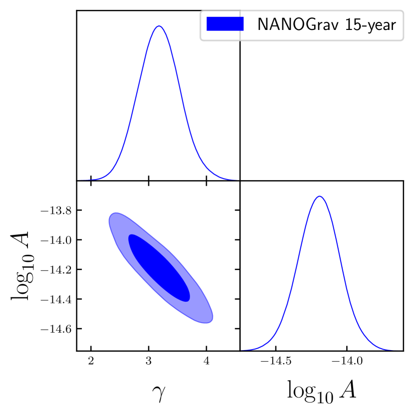
Fitting a model describing an isotropic SGWB characterized by HD correlations, the NANOGrav collaboration inferred the values of the intrinsic-noise amplitude and spectral index appearing in Eq. (11) to be and respectively (both reported at ), at a reference frequency of Agazie et al. (2023a). The joint - posterior is reported in the lower left panel of Fig. 1 of Ref. Agazie et al. (2023a) (blue contours, reference frequency ). It is worth noting that, compared to the 12.5-year signal, the value of is a factor of higher, whereas is significantly lower (as discussed in more detail in the next paragraph), corresponding to a bluer spectrum given the relation between and in Eq. (12). Therefore, one can already expect quantitative differences in the inflationary interpretation compared to my earlier results of Ref. Vagnozzi (2021), going in the direction of a bluer spectrum due to both the smaller value of and the larger value of . This expectation will in fact be confirmed in Sec. IV.
As noted in Ref. Agazie et al. (2023a), the inferred value of is low relative to (and in moderate tension with) the value expected from merging SMBHBs, which lies at the upper boundary of the region. Interestingly a similar “anomaly”, albeit reversed in direction, was observed in the 12.5-year dataset, where was inferred Arzoumanian et al. (2020). In that case, the value lay just outside the lower boundary of the region. However, astrophysical effects can alter the value of arising from merging SMBHBs, and the estimation of itself is sensitive to details in the modeling of intrinsic red noise and of interstellar medium timing delays in a few pulsars. The NANOGrav collaboration performed several robustness and validation tests, and found the inferred values of and to be quite stable against changes in the underlying analysis assumptions: I shall therefore take the consensus results reported in the lower left panel of Fig. 1 of Ref. Agazie et al. (2023a) as the baseline signal for which the viability of an inflationary interpretation will be examined.
In my earlier work of Ref. Vagnozzi (2021) I translated the inferred NANOGrav 12.5-year constraints on and into constraints on and through a simple grid scan. Although this simple method was more than sufficiently accurate to identify the benchmark region of inflationary parameter space required to explain the signal, here I improve the robustness and portability of the analysis method by performing a Bayesian analysis, through a Markov Chain Monte Carlo (MCMC) scan of the parameter space. 777A posteriori, I have cross-checked that repeating the analysis of Ref. Vagnozzi (2021) through an MCMC rather than a grid scan recovers essentially the same results. Specifically, my goal is to derive constraints on the cosmological parameters, with focus on the inflationary parameters and , treating the - posterior distribution inferred by NANOGrav as a likelihood. 888See Ref. Visinelli and Vagnozzi (2019) where a similar simplified approach was adopted and justified by means of Bayes’ theorem, and Appendix A of Ref. Giarè et al. (2023b) which confirms the goodness of the Gaussian approximation I have adopted. To this end, I seek a closed-form approximation for the NANOGrav - joint posterior distribution. I find that the latter is well approximated by a bivariate Gaussian in and , with mean vector and covariance matrix given by:
| (16) |
To test the goodness of this approximation, I run a test MCMC on the 2 parameters and , using the bivariate Gaussian described above as likelihood, and assuming flat wide priors on both parameters. As the priors are flat and no other likelihoods are used, the recovered joint - posterior directly traces the input bivariate Gaussian distribution, and by extension the NANOGrav 15-year joint - posterior for which I am seeking a closed-form approximation. The resulting joint - posterior, alongside the 1D marginalized distributions in and , are shown in Fig. 1. Comparing this to the lower left panel of Fig. 1 of Ref. Agazie et al. (2023a) (blue contours, reference frequency ), I find excellent agreement between the two, confirming the goodness of my approximation, especially for the purpose of pinpointing the (a posteriori rather implausible) benchmark region of inflationary parameter space required to explain the NANOGrav signal.
Having made these considerations, I therefore approximate the NANOGrav log-likelihood as:
| (17) |
where is the vector of derived parameters , where indicates the vector of cosmological parameters, T denotes the transpose operation, and and are respectively the vector of mean values and covariance matrix for the derived parameters and and the covariance matrix discussed earlier and given in Eq. (16). In principle should include all the relevant cosmological parameters governing the amplitude and shape of the inflationary SGWB: , , , , and (or equivalently ). However, as argued earlier in Sec. II, in practice only and have an important effect on the inflationary SGWB signal, whereas the effect of the other parameters is completely subdominant given the level of precision to which they have been determined by current cosmological observations, in particular the Planck satellite. Thus, in what follows I assume , i.e. that the independent cosmological parameters are and . I connect and to the derived parameters and entering the NANOGrav likelihood of Eq. (17) through Eqs. (12,14), fixing all other parameters to their best-fit values as per the Planck 2018 results Aghanim et al. (2020) quoted in Sec. II.
Given the fact that the order of magnitude of the tensor-to-scalar ratio is presently unknown, from a statistical point of view it proves more convenient to work with rather than itself. To sample the joint - posterior distribution in light of the NANOGrav signal, whose information is included by means of the log-likelihood of Eq. (17), I generate MCMC chains through the cosmological sampler MontePython Audren et al. (2013); Brinckmann and Lesgourgues (2019), which I have configured to act as a generic sampler. I impose wide flat priors on both and , and have verified a posteriori that the prior ranges do not cut the posteriors of the two parameters where these are significantly non-zero. In addition, I impose a hard prior on such that , to reflect the current upper limit on (at the same pivot scale at which has been reported) obtained by a joint analysis of Planck, WMAP, BICEP2, Keck Array, and BICEP3 data Ade et al. (2021) (I have check a posteriori that the choice of including this limit has very little effect on my results). I assess the convergence of the generated MCMC chains by using the Gelman-Rubin parameter Gelman and Rubin (1992), and require in order for the MCMC chains to be considered converged.
IV Results and discussions
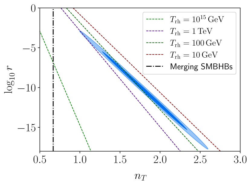
I perform an MCMC run as described above to identify which region of inflationary parameter space can, at face value, explain the NANOGrav 15-year signal. 999Besides the inflationary interpretation I put forward in Ref. Vagnozzi (2021), the NANOGrav 12.5-year signal (and the related PPTA, EPTA, and IPTA signals) stimulated a lot of work devoted to possible theoretical interpretations: for an inevitably limited selection of examples, see e.g. Refs. Ellis and Lewicki (2021); Blasi et al. (2021); Vaskonen and Veermäe (2021); De Luca et al. (2021); Buchmuller et al. (2020); Nakai et al. (2021); Addazi et al. (2021); Kohri and Terada (2021); Ratzinger and Schwaller (2021); Samanta and Datta (2021); Bian et al. (2021); Namba and Suzuki (2020); Neronov et al. (2021); Li et al. (2021a); Sugiyama et al. (2021); Liu et al. (2021); Paul et al. (2021); Zhou et al. (2020); Domènech and Pi (2022); Bhattacharya et al. (2021); Abe et al. (2021); Kitajima et al. (2021); Middleton et al. (2021); Inomata et al. (2021); Tahara and Kobayashi (2020); Chigusa et al. (2021); Pandey (2021); Bigazzi et al. (2021); Ramberg and Visinelli (2021); Cai and Piao (2021); Barman et al. (2020); Chiang and Lu (2021); Atal et al. (2021); Datta et al. (2021); Chen et al. (2021b); Gao and Yang (2021); Li et al. (2021b); Gorghetto et al. (2021); Kawasaki and Nakatsuka (2021); Blanco-Pillado et al. (2021); Sharma (2022); Brandenburg et al. (2021); Hindmarsh et al. (2021); Lazarides et al. (2021); Zhou et al. (2021); Sakharov et al. (2021); Arzoumanian et al. (2021a); Moore and Vecchio (2021); Borah et al. (2021a); Yi and Zhu (2022); Wu et al. (2021); Haque et al. (2021); Liu et al. (2022); Lewicki et al. (2021); Chang and Cui (2022); Buchmuller et al. (2021); Masoud et al. (2021); Casey-Clyde et al. (2022); Li and Shapiro (2021); Cai et al. (2021a); Spanos and Stamou (2021); Khodadi et al. (2021); Wu et al. (2022); Izquierdo-Villalba et al. (2021); Chen et al. (2022); Borah et al. (2021b); Arzoumanian et al. (2021b); Gao (2021); Lin et al. (2023); Benetti et al. (2022); Dunsky et al. (2022); Zhang (2022); Cai and Piao (2022); Roper Pol et al. (2022); Wang (2022a); Ashoorioon et al. (2022); Ahmed et al. (2022); Afzal et al. (2022); Wang (2022b); Cheong et al. (2022); Bernardo and Ng (2023a); Ghoshal et al. (2022); Datta and Samanta (2022); El Bourakadi et al. (2022); Blasi et al. (2023a); Borah et al. (2023a); Saad (2023); Bian et al. (2022); Cai (2023); Arzoumanian et al. (2023); Berbig and Ghoshal (2023); Wu et al. (2023); Dandoy et al. (2023); Bernardo and Ng (2023b); An and Yang (2023); Ferrer et al. (2023); Ghoshal et al. (2023b); Ferrante et al. (2023); Bringmann et al. (2023); Madge et al. (2023); Baldes et al. (2023). The resulting joint - posterior is shown in Fig. 2. Ignoring for the moment the dashed lines associated to different reheating temperatures, I find , completely in line with expectations given the inferred values of . The vertical dot-dashed line at indicates the expected value from merging SMBHBs corresponding to : not surprisingly, it lies out of the region. In addition, I find a very strong negative degeneracy between and , with a correlation coefficient , also not unexpected given that a lower value of can be compensated with a bluer spectrum, and viceversa. From Fig. 2 one also sees that the NANOGrav signal actually points towards rather low values of , as a direct consequence of the very high value of : larger values of would actually lead to the resulting SGWB exceeding the amplitude of the signal detected by NANOGrav. Within this scenario, the resulting inflationary SGWB would be barely detectable by next-generation CMB experiments Abazajian et al. (2016); Ade et al. (2019); Abitbol et al. (2019). As additionally anticipated earlier, the value of the tensor spectral index required to explain the NANOGrav 15-year signal is larger than that required to explain the 12.5-year signal Vagnozzi (2021), as a direct consequence of both the higher value of , as well as the significantly lower value of .
The key point to take away from these results is that explaining the NANOGrav 15-year signal requires a very blue spectrum, which very strongly violates the consistency relation Copeland et al. (1993). Obviously, this cannot be realized within the simplest single-field slow-roll inflationary models. Nevertheless, a number of inflationary (and non-inflationary) models leading to a blue spectrum (or more generally significant deviations from the simplest expectations) have been discussed in recent years: with no claims as to completeness, these models include inflationary models based on phantom fields Piao and Zhang (2004); Liu et al. (2011); Liu and Piao (2012); Dinda et al. (2014); Richarte and Kremer (2017), modifications to gravity Kobayashi et al. (2010); Myrzakulov et al. (2015b); Fujita et al. (2019); Odintsov and Oikonomou (2019); Nojiri et al. (2020a, b); Odintsov and Oikonomou (2020); Nojiri et al. (2020c); Odintsov et al. (2020); Kawai and Kim (2021); Oikonomou (2021); Odintsov et al. (2022b); Odintsov and Oikonomou (2022a, b); Oikonomou (2022a); Odintsov and Oikonomou (2022c); Oikonomou (2022b); Oikonomou and Lymperiadou (2022); Oikonomou (2023a, 2022c) or non-commutative space-times Calcagni and Tsujikawa (2004); Calcagni et al. (2014), breaking of spatial or temporal diffeomorphism invariance Endlich et al. (2013); Cannone et al. (2015); Graef and Brandenberger (2015); Ricciardone and Tasinato (2017); Graef et al. (2017), violations of the null energy condition Baldi et al. (2005), couplings to axionic, gauge, and spin-2 fields Maleknejad and Sheikh-Jabbari (2011); Adshead and Wyman (2012); Maleknejad (2016); Dimastrogiovanni et al. (2017); Adshead et al. (2016); Obata (2017); Nojiri et al. (2019); Iacconi et al. (2020); Oikonomou (2023b) and particle production Cook and Sorbo (2012); Pajer and Peloso (2013); Mukohyama et al. (2014), initial states other than the Bunch-Davies one Ashoorioon et al. (2014), elastic media Gruzinov (2004), higher order effective gravitational action corrections Giarè et al. (2021b), second-order effects Biagetti et al. (2013) (including those associated to the formation of primordial BHs), sound speed resonance effects Cai et al. (2016, 2021b) and finite-time singularities Kleidis and Oikonomou (2016), alternatives to inflation such as string gas cosmology Brandenberger and Vafa (1989); Brandenberger et al. (2007a, b); Stewart and Brandenberger (2008); Brandenberger et al. (2014), ekpyrotic Khoury et al. (2001); Hipolito-Ricaldi et al. (2016) and bouncing Brandenberger (2011) scenarios, and many others (see Ref. Wang and Xue (2014) for a more detailed overview of these scenarios). It is worth noting that, in principle, the inferred value of is not inconsistent with CMB observations alone, as these are unable to place strong constraints on in the absence of a detection of non-zero , or without including additional data (e.g. interferometer-scale limits on the the SGWB amplitude). 101010See e.g. Refs. Meerburg et al. (2015); Cabass et al. (2016); Wang et al. (2017); Graef et al. (2019); Giarè et al. (2019) for examples of works examining constraints on from CMB data, which in the absence of a detection of primordial B-modes are extremely weak due to the degeneracy between and . An alternative approach explored by Ref. Galloni et al. (2023) is to re-parameterize the tensor power spectrum using two different tensor-to-scalar ratios defined at two pivot scales: this “two-scales approach” was shown to improve the constraints on , although when using CMB data alone these constraints remain comparatively weak. See however Ref. Giarè and Renzi (2020) for a different work which argued that constraints on from CMB data might actually be stronger than previously thought.
More importantly, such a blue spectrum has a very strong impact on , and hence on BBN. In Fig. 2, the dashed curves correspond to isocontours of for different values of the reheating temperature (see color coding) and therefore of the frequency cutoff appearing in Eq. (15). The regions to the right of the curves are excluded by the requirement from BBN and CMB considerations (indicative and rather generous upper limit, with the caveats for the CMB discussed in footnote 6). From Fig. 2 it is clear that the inflationary interpretation of the NANOGrav signal is in strong tension with limits on unless the reheating temperature is as low as . Unsurprisingly, this upper limit on the reheating temperature is even stronger than the limit I obtained previously from the 12.5-year dataset, , as a direct result of the bluer spectrum. While low-scale reheating models have been studied for quite a while Kawasaki et al. (2000); Giudice et al. (2001); Hannestad (2004), they are generally less easier to construct, and require e.g. an unusually long period of slow-roll or the existence of long-lived massive particles. It is worth noting that with such a low reheating scale, cosmic neutrinos may not have had time to thermalize completely by the time they decouple – as a consequence, the current relic neutrino energy and number densities may be lower compared to standard expectations de Salas et al. (2015); Gerbino et al. (2017). 111111Given the recent results from the Atacama Cosmology Telescope (ACT) which have inferred a value of lower than expected Aiola et al. (2020), one may in principle be tempted to speculate as to whether an underlying low-reheating scenario may explain these results. See, however, Refs. Handley and Lemos (2021); Giarè et al. (2023c); Zhai et al. (2023); Di Valentino et al. (2023); Giarè et al. (2023d) for discussions on the tension between ACT and Planck for what concerns the determination of parameters such as , , and .
An important caveat to all these results is my choice of treating as a pure power-law from CMB frequencies down to PTA frequencies. While this approximation is widespread (just by way of recent well-known examples, see e.g. Refs. Meerburg et al. (2015); Akrami et al. (2020); Campeti et al. (2021)), it might not be entirely justified when considering probes leading to a wide lever arm in frequency space Giarè and Melchiorri (2021); Kinney (2021). For instance, there are about decades in frequency between CMB and PTA scales, and an additional decades in frequency between PTA and current interferometer scales. To address this point, what would ultimately be required is to estimate the theoretical uncertainties in the predictions for inflationary parameters in a way as potential-agnostic as possible (for instance through Monte Carlo inflation flow potential reconstruction, see e.g. Refs. Kinney and Riotto (2006); Caligiuri et al. (2015)). Nevertheless, for what concerns the present work, treating the primordial tensor spectrum as being a pure power-law between CMB and PTA scales might actually not be too bad an approximation: in this respect, see for example Fig. 5 in Ref. Kinney (2021), where PTA scales correspond to , where the relative deviation from the pure power-law extrapolation for an example inflationary potential is actually rather small. Nevertheless, extending this treatment down to interferometer scales and beyond is clearly not reasonable (as is clear from the same Figure). Overall this question, while important, goes well beyond the scope of my work, and I therefore defer it to future studies.
A somewhat observationally more relevant point related to the above is that the blue spectrum described earlier, if naïvely extrapolated down to interferometer scales (which, repetita juvant, should not be done in any case!), would inevitably violate upper limits on the SGWB amplitude on interferometer scales, where Advanced LIGO/Advanced Virgo set the upper limit at Abbott et al. (2021). An obvious and well-motivated way to address this problem is to envisage the existence of a break in the tensor power spectrum, which in the simplest case would therefore be described by a broken power-law. Such an approach was discussed in detail in Ref. Benetti et al. (2022), to which I refer the reader for further details. Here, I simply note that a wide variety of well-motivated scenarios naturally give rise to a break in the tensor power spectrum: such scenarios include but are not limited to a non-instantaneous reheating process (possibly with a low reheating scale), an early period of non-standard expansion (e.g. an early matter domination phase, or a kination phase), late-time entropy injection, models where the inflaton is coupled to gauge fields, and alternatives to inflation. Whichever mechanism one chooses to invoke, the break needs to take place at frequencies , and the post-break spectrum needs to be sufficiently red in order for the SGWB amplitude to be low enough on interferometer scales (see Ref. Benetti et al. (2022) for further details on this phenomenological approach).
The required reheating scale required for an inflationary interpretation of the NANOGrav 15-year signal to be viable at face value is extremely low, below the electroweak scale. While this is in principle allowed by cosmological probes, which only require de Salas et al. (2015), realizing it in practice from the particle point of view is more challenging (for instance, it is unclear whether electroweak symmetry breaking can proceed successfully as usual, although on the other hand such a scenario may facilitate the generation of a baryon asymmetry). Finally, it is worth noting that the reheating scale can be lowered even in the absence of new physics, through effects such as “Higgs blocking” Freese et al. (2018); Litsa et al. (2021, 2023).
The biggest challenge for an inflationary interpretation of the NANOGrav 15-year results, however, is the extremely blue spectrum required to fit the signal, with close to . As one sees from Eq. (6), even within effective phantom inflationary scenarios, the value can only be reached asymptotically if one requires (it can be reached for positive values of , but these are not of interest to an inflationary discussion). Nevertheless, even just getting close to within phantom inflationary models would require considering very deep phantom models: needless to say, such models are theoretically problematic and hard to achieve in a controlled setting. Just by way of example, from Eq. (6) one sees that obtaining requires , whereas obtaining requires – both correspond to values deep in the phantom regime, and therefore theoretically very problematic. Motivated by the 2014 BICEP-2 signal, Ref. Wang and Xue (2014) discussed a number of inflationary scenarios leading to blue tensor spectra, including the ones discussed earlier in this Section: for most of these models, it was found that reaching values of the tensor spectral index is extremely hard if not impossible altogether. In a more generic setting, this is also further supported by the findings of Ref. Giarè et al. (2023a), where based on an extension of the flow approach it was shown that most of the mechanisms proposed to obtain a blue spectrum (especially those which can be cast in terms of additional effective field theory operators) actually only support for few e-folds, which is quite different from what is required to explain the NANOGrav signal. This further supports the untenability of an inflationary interpretation of the NANOGrav signal.
An explicit phantom inflationary model is just one way of violating the null energy condition (NEC), which is a well-motivated possibility to obtain a blue spectrum. Besides explicit phantom inflationary models, the NEC can be violated within models based on modified gravity, and an interesting model in this sense is the G-inflation model Kobayashi et al. (2010), based on a Galileon field (see also Refs. Deffayet et al. (2009); He et al. (2016)). This allows for NEC violation at the cosmological background level without introducing a ghost in the scalar sector. However, in its simplest incarnation this model is problematic because a) the scalar and tensor spectra tilt in the same direction, so a very blue tensor spectrum would require a very blue scalar spectrum, strongly excluded by observations, and b) the bluer the tensor spectrum, the larger the level of equilateral non-Gaussianity predicted (due to non-linear self-interactions of the Galileon field), which in the case of are safely ruled out. Another possibility involves perturbations generated from a non-Bunch-Davies vacuum, although again achieving a large tensor spectral index comes at the price of introducing a significant level of (folded) non-Gaussianity both in the scalar and tensor sectors, with the former excluded by observations Wang and Xue (2014). Remaining within the inflationary realm, and in the context of the non-standard scenarios discussed earlier in this Section, one finds that either is positive but too small (certainly not as required by the NANOGrav signal), or achieving large comes at the price of a significant level of non-Gaussianities, already excluded by observations. 121212One possible interesting exception is the non-local extension of Starobinsky inflation, itself motivated by attempts to construct a 4-dimensional theory of quantum gravity, and whose phenomenology was recently studied in Refs. Koshelev et al. (2016, 2018, 2020a, 2020b, 2022a, 2022b, 2023). All these considerations bring me to the general conclusion that an inflationary interpretation of the NANOGrav signal, and by extension of the signal recently observed by EPTA+InPTA, PPTA, and CPTA (given the broad agreement between all four signals) is hardly tenable.
Before closing, I briefly discuss predictions for within alternatives to inflation. It is worth noting that one of the first predictions for a blue tensor spectrum came from string gas cosmology Brandenberger and Vafa (1989); Brandenberger et al. (2007a), wherein the universe emerged from a string Hagedorn phase at a nearly constant temperature, until the decay of the string winding modes allowed for the expansion of the Universe. Within string gas cosmology, one finds Brandenberger et al. (2014); Wang and Xue (2014):
| (18) |
which is not suppressed by the slow-roll parameters, and therefore clearly has a hard time explaining the value of required by the NANOGrav signal, given that constraints on the scalar spectral index from Planck imply . 131313A related scenario was studied in Ref. Biswas et al. (2014), where the possibility of producing primordial fluctuations from statistical thermal fluctuations within string gas cosmology was explored. In particular, blue GWs are produced during a stringy thermal contracting phase at temperatures higher than the Hagedorn temperature. However, this scenario predicts , which is at odds with the NANOGrav signal.
A more interesting possibility is the so-called “old ekpyrotic” scenario Khoury et al. (2001) (see also Refs. Khoury et al. (2002); Buchbinder et al. (2007); Lehners (2008); Oikonomou (2015); Odintsov et al. (2015)), wherein the Universe starts in a cold, very slowly contracting state, after which the collision of a brane in the bulk space with a bounding orbifold plane starts the hot Big Bang expansion era. The ekpyrotic model predicts a quasi-scale-invariant spectrum of scalar perturbations and a very blue tensor spectrum with Boyle et al. (2004). However, on cosmological scales the amplitude of tensor modes is highly suppressed Khoury et al. (2001); Boyle et al. (2004), so that despite the large blue tilt, the resulting SGWB remains well below the detection threshold even on PTA scales Boyle et al. (2004); Calcagni and Kuroyanagi (2021). While the “new ekpyrotic” scenario Brandenberger and Wang (2020a, b); Brandenberger et al. (2020) avoids these problems, it also predicts a relation between and of the same form as Eq. (18), and therefore a tensor spectrum which does not carry a strong enough blue tilt to explain the signal observed by PTA experiments.
V Conclusions
A number of pulsar timing array (PTA) experiments (NANOGrav, EPTA+InPTA, PPTA, and CPTA) have recently confirmed the detection of a common-spectrum low-frequency stochastic signal across the pulsars in their latest datasets, with the additional compelling evidence of Hellings-Downs inter-pulsar correlations, achieving the first convincing detection of a stochastic gravitational wave background (SGWB) in the frequency range Agazie et al. (2023a); Antoniadis et al. (2023a); Reardon et al. (2023a); Xu et al. (2023); Agazie et al. (2023b, c); Afzal et al. (2023); Agazie et al. (2023d, e, f); Johnson et al. (2023); Antoniadis et al. (2023b, c, d, e); Smarra et al. (2023); Reardon et al. (2023b); Zic et al. (2023). This has officially broadened the horizons of GW astronomy, and the quest is now open for determining the origin of these signals. An unresolved background of merging supermassive black hole binaries is a natural candidate explanation, whereas another exciting possibility entails a cosmological origin. While other types of observations (for instance the detection of anisotropies Bartolo et al. (2019, 2020, 2022); Galloni et al. (2022); Schulze et al. (2023)) are ultimately required to discern between these two possibilities, it is interesting to examine whether cosmological explanations are consistent with the currently reported characteristics of the signal. In this work, focusing for concreteness and simplicity on the NANOGrav 15-year signal (given that the signals observed in all four PTA experiments are mutually consistent), I have tested the viability of an inflationary SGWB interpretation, given the uttermost theoretical importance of an inflationary era as a source of cosmological GWs.
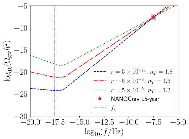
The main outcomes of my analysis are summarized in Fig. 2 and Fig. 3. Compared to the earlier NANOGrav 12.5-year results, for which an inflationary interpretation was in principle not unreasonable Vagnozzi (2021), an inflationary origin for the NANOGrav 15-year signal appears much less tenable. Firstly, the spectrum required to explain the signal is extremely blue (), to an extent which, while theoretically not impossible to obtain, presents huge challenges within inflationary settings. As discussed in Sec. IV, obtaining within inflationary models is extremely challenging (and at the very least requires moving far from the single-field slow-roll paradigm), and the least unlikely realizations all tend to predict sizeable non-Gaussianities, which have not been detected. Alternatives to inflation can also provide a source for such a blue-tilted SGWB spectrum, with an ekpyrotic phase being a particularly intriguing possibility in this sense, given the fact that such scenarios naturally predict , although in this case the expected amplitude of the signal is far too small. Returning to the inflationary realm, another difficulty concerns the fact that the required reheating scale has to be extremely low, below the electroweak scale, posing additional difficulties on the model-building side. 141414Even if an inflationary model which overcomes such difficulties can be constructed, the blue spectrum would anyhow require a break at frequencies above PTA scales, in order not to violate upper limits on the SGWB amplitude on interferometer scales (see e.g. the model-agnostic approach in Ref. Benetti et al. (2022)). Finally, I have provided explicit expressions for a bivariate Gaussian approximation to the joint posterior distribution for the intrinsic-noise amplitude and spectral index inferred from the NANOGrav signal. This can facilitate extending similar simplified likelihood analyses to different underlying theoretical signals for which a prediction for the amplitude and spectral index can easily be obtained.
Overall, it is safe to say that an inflationary interpretation of the signals reported in June 2023 by various PTA experiments appears exceptionally unlikely. Other cosmological sources, such as GWs generated by a network of cosmic strings or associated to the formation of primordial black holes, may provide a better explanation for the signal, and I expect that such possibilities will be examined in significant detail elsewhere in the literature. 151515Besides the NANOGrav Afzal et al. (2023) and EPTA Antoniadis et al. (2023e) official publications on searches for new physics, see e.g. Refs. Liu (2023); King et al. (2023); Zu et al. (2023); Han et al. (2023); Lambiase et al. (2023); Ellis et al. (2023a); Guo et al. (2023); Megias et al. (2023); Fujikura et al. (2023); Yang et al. (2023a); Li et al. (2023); Deng et al. (2023); Franciolini et al. (2023a); Shen et al. (2023); Kitajima et al. (2023); Ellis et al. (2023b); Franciolini et al. (2023b); Wang et al. (2023a); Ghoshal and Strumia (2023); Bai et al. (2023); Addazi et al. (2023); Athron et al. (2023); Oikonomou (2023c); Kitajima and Nakayama (2023); Huang et al. (2023); Eichhorn et al. (2023); Buchmueller et al. (2023); Lazarides et al. (2023); Broadhurst et al. (2023); Cai et al. (2023); Yang et al. (2023b); Blasi et al. (2023b); Inomata et al. (2023); Depta et al. (2023); Gouttenoire and Vitagliano (2023); Borah et al. (2023b); Wang et al. (2023b); Murai and Yin (2023); Datta (2023); Barman et al. (2023); Bi et al. (2023); Lu and Chiang (2023); Xiao et al. (2023); Li and Xie (2023); Zhang et al. (2023); Anchordoqui et al. (2023); Liu et al. (2023); Konoplya and Zhidenko (2023); Chowdhury et al. (2023); Niu and Rahat (2023), for examples of works connecting the PTA signals to a variety of fundamental physics models. Looking beyond, it will be interesting to see whether the characteristics of the signal will be confirmed by future PTA observations, e.g. the forthcoming IPTA Data Release 3, which will include a total of 80 pulsars observed for up to 24 years, with a considerably improved sensitivity to spatial correlations and spectral resolutions compared to single-PTA datasets such as the ones considered here. These datasets will help clarify the origin of the SGWB, settling the question of whether the latter is astrophysical or cosmological in origin. Regardless of the outcome, it is beyond doubt that PTA experiments are opening a new, exciting window onto GWs produced in the early Universe (including potentially during inflation), at energy scales and physical regimes which are completely inaccessible down on Earth: the era of nHz GW astronomy is upon us.
Note added
I have independently started this work in preparation for the much anticipated public announcement of NANOGrav in coordination with other PTA experiment on June 29, 2023. Inevitably, by then NANOGrav Afzal et al. (2023) and EPTA Antoniadis et al. (2023e) had already explored an inflationary interpretation of their results. However, they considered slightly different parametrizations and ingredients (e.g. non-instantaneous reheating), and conversely my work discusses in more detail the difficulties associated to an inflationary origin of the signals, which are only alluded to by NANOGrav. Our results are in good overall agreement, as we all agree on the need for a very blue spectrum and a very low reheating temperature. This provides a valuable and independent cross-check, whereas our discussions of the results nicely complement each other.
Acknowledgements.
I thank William Giarè and Will Kinney for many useful discussions around the subject of this work. This publication is based upon work from the COST Action CA21136 “Addressing observational tensions in cosmology with systematics and fundamental physics (CosmoVerse), supported by COST (European Cooperation in Science and Technology).References
- Caprini and Figueroa (2018) C. Caprini and D. G. Figueroa, Class. Quant. Grav. 35, 163001 (2018), arXiv:1801.04268 [astro-ph.CO] .
- Renzini et al. (2022) A. I. Renzini, B. Goncharov, A. C. Jenkins, and P. M. Meyers, Galaxies 10, 34 (2022), arXiv:2202.00178 [gr-qc] .
- Siemens et al. (2007) X. Siemens, V. Mandic, and J. Creighton, Phys. Rev. Lett. 98, 111101 (2007), arXiv:astro-ph/0610920 .
- Caprini et al. (2010) C. Caprini, R. Durrer, and X. Siemens, Phys. Rev. D 82, 063511 (2010), arXiv:1007.1218 [astro-ph.CO] .
- Ramberg and Visinelli (2019) N. Ramberg and L. Visinelli, Phys. Rev. D 99, 123513 (2019), arXiv:1904.05707 [astro-ph.CO] .
- Caprini et al. (2020) C. Caprini et al., JCAP 03, 024 (2020), arXiv:1910.13125 [astro-ph.CO] .
- Ellis et al. (2020) J. Ellis, M. Lewicki, and J. M. No, JCAP 07, 050 (2020), arXiv:2003.07360 [hep-ph] .
- Rajagopal and Romani (1995) M. Rajagopal and R. W. Romani, Astrophys. J. 446, 543 (1995), arXiv:astro-ph/9412038 .
- Jaffe and Backer (2003) A. H. Jaffe and D. C. Backer, Astrophys. J. 583, 616 (2003), arXiv:astro-ph/0210148 .
- Wyithe and Loeb (2003) J. S. B. Wyithe and A. Loeb, Astrophys. J. 590, 691 (2003), arXiv:astro-ph/0211556 .
- Sesana et al. (2004) A. Sesana, F. Haardt, P. Madau, and M. Volonteri, Astrophys. J. 611, 623 (2004), arXiv:astro-ph/0401543 .
- Burke-Spolaor et al. (2019) S. Burke-Spolaor et al., Astron. Astrophys. Rev. 27, 5 (2019), arXiv:1811.08826 [astro-ph.HE] .
- Sazhin (1978) M. V. Sazhin, Soviet Ast. 22, 36 (1978).
- Detweiler (1979) S. L. Detweiler, Astrophys. J. 234, 1100 (1979).
- Hobbs and Dai (2017) G. Hobbs and S. Dai, Natl. Sci. Rev. 4, 707 (2017), arXiv:1707.01615 [astro-ph.IM] .
- Arzoumanian et al. (2020) Z. Arzoumanian et al. (NANOGrav), Astrophys. J. Lett. 905, L34 (2020), arXiv:2009.04496 [astro-ph.HE] .
- Goncharov et al. (2021) B. Goncharov et al., Astrophys. J. Lett. 917, L19 (2021), arXiv:2107.12112 [astro-ph.HE] .
- Chen et al. (2021a) S. Chen et al., Mon. Not. Roy. Astron. Soc. 508, 4970 (2021a), arXiv:2110.13184 [astro-ph.HE] .
- Antoniadis et al. (2022) J. Antoniadis et al., Mon. Not. Roy. Astron. Soc. 510, 4873 (2022), arXiv:2201.03980 [astro-ph.HE] .
- Pol et al. (2021) N. S. Pol et al. (NANOGrav), Astrophys. J. Lett. 911, L34 (2021), arXiv:2010.11950 [astro-ph.HE] .
- Romano et al. (2021) J. D. Romano, J. S. Hazboun, X. Siemens, and A. M. Archibald, Phys. Rev. D 103, 063027 (2021), arXiv:2012.03804 [gr-qc] .
- Hellings and Downs (1983) R. w. Hellings and G. s. Downs, Astrophys. J. Lett. 265, L39 (1983).
- Goncharov et al. (2022) B. Goncharov et al., Astrophys. J. 932, L22 (2022), arXiv:2206.03766 [gr-qc] .
- Zic et al. (2022) A. Zic et al., Mon. Not. Roy. Astron. Soc. 516, 410 (2022), arXiv:2207.12237 [astro-ph.HE] .
- Tiburzi et al. (2016) C. Tiburzi, G. Hobbs, M. Kerr, W. Coles, S. Dai, R. Manchester, A. Possenti, R. Shannon, and X. You, Mon. Not. Roy. Astron. Soc. 455, 4339 (2016), arXiv:1510.02363 [astro-ph.IM] .
- Agazie et al. (2023a) G. Agazie et al. (NANOGrav), Astrophys. J. Lett. 951, L8 (2023a), arXiv:2306.16213 [astro-ph.HE] .
- Antoniadis et al. (2023a) J. Antoniadis et al., (2023a), arXiv:2306.16214 [astro-ph.HE] .
- Reardon et al. (2023a) D. J. Reardon et al., Astrophys. J. Lett. 951, L6 (2023a), arXiv:2306.16215 [astro-ph.HE] .
- Xu et al. (2023) H. Xu et al., Res. Astron. Astrophys. 23, 075026 (2023), arXiv:2306.16216 [astro-ph.HE] .
- Agazie et al. (2023b) G. Agazie et al. (NANOGrav), Astrophys. J. Lett. 951, L9 (2023b), arXiv:2306.16217 [astro-ph.HE] .
- Agazie et al. (2023c) G. Agazie et al. (NANOGrav), Astrophys. J. Lett. 951, L10 (2023c), arXiv:2306.16218 [astro-ph.HE] .
- Afzal et al. (2023) A. Afzal et al. (NANOGrav), Astrophys. J. Lett. 951, L11 (2023), arXiv:2306.16219 [astro-ph.HE] .
- Agazie et al. (2023d) G. Agazie et al. (NANOGrav), (2023d), arXiv:2306.16220 [astro-ph.HE] .
- Agazie et al. (2023e) G. Agazie et al. (NANOGrav), (2023e), arXiv:2306.16221 [astro-ph.HE] .
- Agazie et al. (2023f) G. Agazie et al. (NANOGrav), (2023f), arXiv:2306.16222 [astro-ph.HE] .
- Johnson et al. (2023) A. D. Johnson et al. (NANOGrav), (2023), arXiv:2306.16223 [astro-ph.HE] .
- Antoniadis et al. (2023b) J. Antoniadis et al., (2023b), 10.1051/0004-6361/202346841, arXiv:2306.16224 [astro-ph.HE] .
- Antoniadis et al. (2023c) J. Antoniadis et al., (2023c), arXiv:2306.16225 [astro-ph.HE] .
- Antoniadis et al. (2023d) J. Antoniadis et al., (2023d), arXiv:2306.16226 [astro-ph.HE] .
- Antoniadis et al. (2023e) J. Antoniadis et al., (2023e), arXiv:2306.16227 [astro-ph.CO] .
- Smarra et al. (2023) C. Smarra et al., (2023), arXiv:2306.16228 [astro-ph.HE] .
- Reardon et al. (2023b) D. J. Reardon et al., Astrophys. J. Lett. 951, L7 (2023b), arXiv:2306.16229 [astro-ph.HE] .
- Zic et al. (2023) A. Zic et al., (2023), arXiv:2306.16230 [astro-ph.HE] .
- Kazanas (1980) D. Kazanas, Astrophys. J. Lett. 241, L59 (1980).
- Starobinsky (1980) A. A. Starobinsky, Phys. Lett. B 91, 99 (1980).
- Sato (1981) K. Sato, Phys. Lett. B 99, 66 (1981).
- Guth (1981) A. H. Guth, Phys. Rev. D 23, 347 (1981).
- Mukhanov and Chibisov (1981) V. F. Mukhanov and G. V. Chibisov, JETP Lett. 33, 532 (1981).
- Linde (1982) A. D. Linde, Phys. Lett. B 108, 389 (1982).
- Albrecht and Steinhardt (1982) A. Albrecht and P. J. Steinhardt, Phys. Rev. Lett. 48, 1220 (1982).
- Ijjas et al. (2013) A. Ijjas, P. J. Steinhardt, and A. Loeb, Phys. Lett. B 723, 261 (2013), arXiv:1304.2785 [astro-ph.CO] .
- Ijjas et al. (2014) A. Ijjas, P. J. Steinhardt, and A. Loeb, Phys. Lett. B 736, 142 (2014), arXiv:1402.6980 [astro-ph.CO] .
- Obied et al. (2018) G. Obied, H. Ooguri, L. Spodyneiko, and C. Vafa, (2018), arXiv:1806.08362 [hep-th] .
- Agrawal et al. (2018) P. Agrawal, G. Obied, P. J. Steinhardt, and C. Vafa, Phys. Lett. B 784, 271 (2018), arXiv:1806.09718 [hep-th] .
- Achúcarro and Palma (2019) A. Achúcarro and G. A. Palma, JCAP 02, 041 (2019), arXiv:1807.04390 [hep-th] .
- Garg and Krishnan (2019) S. K. Garg and C. Krishnan, JHEP 11, 075 (2019), arXiv:1807.05193 [hep-th] .
- Kehagias and Riotto (2018) A. Kehagias and A. Riotto, Fortsch. Phys. 66, 1800052 (2018), arXiv:1807.05445 [hep-th] .
- Kinney et al. (2019) W. H. Kinney, S. Vagnozzi, and L. Visinelli, Class. Quant. Grav. 36, 117001 (2019), arXiv:1808.06424 [astro-ph.CO] .
- Ooguri et al. (2019) H. Ooguri, E. Palti, G. Shiu, and C. Vafa, Phys. Lett. B 788, 180 (2019), arXiv:1810.05506 [hep-th] .
- Palti (2019) E. Palti, Fortsch. Phys. 67, 1900037 (2019), arXiv:1903.06239 [hep-th] .
- Bedroya et al. (2020) A. Bedroya, R. Brandenberger, M. Loverde, and C. Vafa, Phys. Rev. D 101, 103502 (2020), arXiv:1909.11106 [hep-th] .
- Geng (2020) H. Geng, Phys. Lett. B 805, 135430 (2020), arXiv:1910.14047 [hep-th] .
- Trivedi (2023) O. Trivedi, Int. J. Mod. Phys. D 32, 2250130 (2023), arXiv:2008.05474 [hep-th] .
- Anchordoqui et al. (2021) L. A. Anchordoqui, I. Antoniadis, D. Lüst, and J. F. Soriano, Phys. Rev. D 103, 123537 (2021), arXiv:2103.07982 [hep-th] .
- Gashti et al. (2022) S. N. Gashti, J. Sadeghi, and B. Pourhassan, Astropart. Phys. 139, 102703 (2022), arXiv:2202.06381 [astro-ph.CO] .
- Martin et al. (2014a) J. Martin, C. Ringeval, and V. Vennin, Phys. Dark Univ. 5-6, 75 (2014a), arXiv:1303.3787 [astro-ph.CO] .
- Benetti (2013) M. Benetti, Phys. Rev. D 88, 087302 (2013), arXiv:1308.6406 [astro-ph.CO] .
- Martin et al. (2014b) J. Martin, C. Ringeval, R. Trotta, and V. Vennin, JCAP 03, 039 (2014b), arXiv:1312.3529 [astro-ph.CO] .
- Creminelli et al. (2014) P. Creminelli, D. López Nacir, M. Simonović, G. Trevisan, and M. Zaldarriaga, Phys. Rev. Lett. 112, 241303 (2014), arXiv:1404.1065 [astro-ph.CO] .
- Dai et al. (2014) L. Dai, M. Kamionkowski, and J. Wang, Phys. Rev. Lett. 113, 041302 (2014), arXiv:1404.6704 [astro-ph.CO] .
- Rinaldi et al. (2014) M. Rinaldi, G. Cognola, L. Vanzo, and S. Zerbini, JCAP 08, 015 (2014), arXiv:1406.1096 [gr-qc] .
- Rinaldi et al. (2015) M. Rinaldi, G. Cognola, L. Vanzo, and S. Zerbini, Phys. Rev. D 91, 123527 (2015), arXiv:1410.0631 [gr-qc] .
- Myrzakulov et al. (2015a) R. Myrzakulov, L. Sebastiani, and S. Zerbini, Eur. Phys. J. C 75, 215 (2015a), arXiv:1502.04432 [gr-qc] .
- Rinaldi et al. (2016) M. Rinaldi, L. Vanzo, S. Zerbini, and G. Venturi, Phys. Rev. D 93, 024040 (2016), arXiv:1505.03386 [hep-th] .
- Escudero et al. (2016) M. Escudero, H. Ramírez, L. Boubekeur, E. Giusarma, and O. Mena, JCAP 02, 020 (2016), arXiv:1509.05419 [astro-ph.CO] .
- Benetti and Alcaniz (2016) M. Benetti and J. S. Alcaniz, Phys. Rev. D 94, 023526 (2016), arXiv:1604.08156 [astro-ph.CO] .
- Benetti et al. (2016) M. Benetti, S. J. Landau, and J. S. Alcaniz, JCAP 12, 035 (2016), arXiv:1610.03091 [astro-ph.CO] .
- Benetti and Ramos (2017) M. Benetti and R. O. Ramos, Phys. Rev. D 95, 023517 (2017), arXiv:1610.08758 [astro-ph.CO] .
- Guo and Zhang (2017) R.-Y. Guo and X. Zhang, Eur. Phys. J. C 77, 882 (2017), arXiv:1704.04784 [astro-ph.CO] .
- Campista et al. (2017) M. Campista, M. Benetti, and J. Alcaniz, JCAP 09, 010 (2017), arXiv:1705.08877 [astro-ph.CO] .
- Ni et al. (2018) S. Ni, H. Li, T. Qiu, W. Zheng, and X. Zhang, Eur. Phys. J. C 78, 608 (2018), arXiv:1707.05570 [astro-ph.CO] .
- Santos da Costa et al. (2018) S. Santos da Costa, M. Benetti, and J. Alcaniz, JCAP 03, 004 (2018), arXiv:1710.01613 [astro-ph.CO] .
- Park and Ratra (2019) C.-G. Park and B. Ratra, Astrophys. J. 882, 158 (2019), arXiv:1801.00213 [astro-ph.CO] .
- Guo et al. (2019) R.-Y. Guo, L. Zhang, J.-F. Zhang, and X. Zhang, Sci. China Phys. Mech. Astron. 62, 30411 (2019), arXiv:1801.02187 [astro-ph.CO] .
- Di Valentino and Mersini-Houghton (2019) E. Di Valentino and L. Mersini-Houghton, Symmetry 11, 520 (2019), arXiv:1807.10833 [astro-ph.CO] .
- Chowdhury et al. (2019) D. Chowdhury, J. Martin, C. Ringeval, and V. Vennin, Phys. Rev. D 100, 083537 (2019), arXiv:1902.03951 [astro-ph.CO] .
- Benetti et al. (2019) M. Benetti, L. Graef, and R. O. Ramos, JCAP 10, 066 (2019), arXiv:1907.03633 [astro-ph.CO] .
- Haro et al. (2020) J. Haro, J. Amorós, and S. Pan, Eur. Phys. J. C 80, 404 (2020), arXiv:1908.01516 [gr-qc] .
- Guo et al. (2020) R.-Y. Guo, J.-F. Zhang, and X. Zhang, Sci. China Phys. Mech. Astron. 63, 290406 (2020), arXiv:1910.13944 [astro-ph.CO] .
- Li et al. (2020) H.-H. Li, G. Ye, Y. Cai, and Y.-S. Piao, Phys. Rev. D 101, 063527 (2020), arXiv:1911.06148 [gr-qc] .
- Aich et al. (2020) M. Aich, Y.-Z. Ma, W.-M. Dai, and J.-Q. Xia, Phys. Rev. D 101, 063536 (2020), arXiv:1912.00995 [astro-ph.CO] .
- Braglia et al. (2020) M. Braglia, D. K. Hazra, L. Sriramkumar, and F. Finelli, JCAP 08, 025 (2020), arXiv:2004.00672 [astro-ph.CO] .
- Cicoli and Di Valentino (2020) M. Cicoli and E. Di Valentino, Phys. Rev. D 102, 043521 (2020), arXiv:2004.01210 [astro-ph.CO] .
- Keeley et al. (2020) R. E. Keeley, A. Shafieloo, D. K. Hazra, and T. Souradeep, JCAP 09, 055 (2020), arXiv:2006.12710 [astro-ph.CO] .
- Santos da Costa et al. (2021) S. Santos da Costa, M. Benetti, R. M. P. Neves, F. A. Brito, R. Silva, and J. S. Alcaniz, Eur. Phys. J. Plus 136, 84 (2021), arXiv:2007.09211 [astro-ph.CO] .
- Rodrigues et al. (2021) J. G. Rodrigues, S. Santos da Costa, and J. S. Alcaniz, Phys. Lett. B 815, 136156 (2021), arXiv:2007.10763 [astro-ph.CO] .
- Vagnozzi et al. (2021a) S. Vagnozzi, E. Di Valentino, S. Gariazzo, A. Melchiorri, O. Mena, and J. Silk, Phys. Dark Univ. 33, 100851 (2021a), arXiv:2010.02230 [astro-ph.CO] .
- Neves et al. (2022) R. M. P. Neves, S. Santos Da Costa, F. A. Brito, and J. S. Alcaniz, JCAP 07, 024 (2022), arXiv:2011.05264 [hep-th] .
- Vagnozzi et al. (2021b) S. Vagnozzi, A. Loeb, and M. Moresco, Astrophys. J. 908, 84 (2021b), arXiv:2011.11645 [astro-ph.CO] .
- Ye et al. (2021) G. Ye, B. Hu, and Y.-S. Piao, Phys. Rev. D 104, 063510 (2021), arXiv:2103.09729 [astro-ph.CO] .
- Dhawan et al. (2021) S. Dhawan, J. Alsing, and S. Vagnozzi, Mon. Not. Roy. Astron. Soc. 506, L1 (2021), arXiv:2104.02485 [astro-ph.CO] .
- Stein and Kinney (2022) N. K. Stein and W. H. Kinney, JCAP 01, 022 (2022), arXiv:2106.02089 [astro-ph.CO] .
- Forconi et al. (2021) M. Forconi, W. Giarè, E. Di Valentino, and A. Melchiorri, Phys. Rev. D 104, 103528 (2021), arXiv:2110.01695 [astro-ph.CO] .
- dos Santos et al. (2022) F. B. M. dos Santos, S. Santos da Costa, R. Silva, M. Benetti, and J. Alcaniz, JCAP 06, 001 (2022), arXiv:2110.14758 [astro-ph.CO] .
- Cabass et al. (2022a) G. Cabass, M. M. Ivanov, O. H. E. Philcox, M. Simonović, and M. Zaldarriaga, Phys. Rev. Lett. 129, 021301 (2022a), arXiv:2201.07238 [astro-ph.CO] .
- Ye and Piao (2022) G. Ye and Y.-S. Piao, Phys. Rev. D 106, 043536 (2022), arXiv:2202.10055 [astro-ph.CO] .
- Antony et al. (2023) A. Antony, F. Finelli, D. K. Hazra, and A. Shafieloo, Phys. Rev. Lett. 130, 111001 (2023), arXiv:2202.14028 [astro-ph.CO] .
- Cabass et al. (2022b) G. Cabass, M. M. Ivanov, O. H. E. Philcox, M. Simonović, and M. Zaldarriaga, Phys. Rev. D 106, 043506 (2022b), arXiv:2204.01781 [astro-ph.CO] .
- Ye et al. (2022) G. Ye, J.-Q. Jiang, and Y.-S. Piao, Phys. Rev. D 106, 103528 (2022), arXiv:2205.02478 [astro-ph.CO] .
- Ghoshal et al. (2023a) A. Ghoshal, D. Mukherjee, and M. Rinaldi, JHEP 05, 023 (2023a), arXiv:2205.06475 [gr-qc] .
- Gangopadhyay et al. (2023) M. R. Gangopadhyay, H. A. Khan, and Yogesh, Phys. Dark Univ. 40, 101177 (2023), arXiv:2205.15261 [astro-ph.CO] .
- Montefalcone et al. (2023a) G. Montefalcone, V. Aragam, L. Visinelli, and K. Freese, Phys. Rev. D 107, 063543 (2023a), arXiv:2209.14908 [gr-qc] .
- Stein and Kinney (2023) N. K. Stein and W. H. Kinney, JCAP 03, 027 (2023), arXiv:2210.05757 [astro-ph.CO] .
- Cabass et al. (2023) G. Cabass, M. M. Ivanov, and O. H. E. Philcox, Phys. Rev. D 107, 023523 (2023), arXiv:2210.16320 [astro-ph.CO] .
- Montefalcone et al. (2023b) G. Montefalcone, V. Aragam, L. Visinelli, and K. Freese, JCAP 03, 002 (2023b), arXiv:2212.04482 [gr-qc] .
- Abazajian et al. (2016) K. N. Abazajian et al. (CMB-S4), (2016), arXiv:1610.02743 [astro-ph.CO] .
- Ade et al. (2019) P. Ade et al. (Simons Observatory), JCAP 02, 056 (2019), arXiv:1808.07445 [astro-ph.CO] .
- Abitbol et al. (2019) M. H. Abitbol et al. (Simons Observatory), Bull. Am. Astron. Soc. 51, 147 (2019), arXiv:1907.08284 [astro-ph.IM] .
- Kamionkowski and Kovetz (2016) M. Kamionkowski and E. D. Kovetz, Ann. Rev. Astron. Astrophys. 54, 227 (2016), arXiv:1510.06042 [astro-ph.CO] .
- Vagnozzi (2021) S. Vagnozzi, Mon. Not. Roy. Astron. Soc. 502, L11 (2021), arXiv:2009.13432 [astro-ph.CO] .
- Zhao et al. (2013) W. Zhao, Y. Zhang, X.-P. You, and Z.-H. Zhu, Phys. Rev. D 87, 124012 (2013), arXiv:1303.6718 [astro-ph.CO] .
- Liu et al. (2016) X.-J. Liu, W. Zhao, Y. Zhang, and Z.-H. Zhu, Phys. Rev. D 93, 024031 (2016), arXiv:1509.03524 [astro-ph.CO] .
- Kuroyanagi et al. (2009) S. Kuroyanagi, T. Chiba, and N. Sugiyama, Phys. Rev. D 79, 103501 (2009), arXiv:0804.3249 [astro-ph] .
- Kuroyanagi et al. (2011a) S. Kuroyanagi, T. Chiba, and N. Sugiyama, Phys. Rev. D 83, 043514 (2011a), arXiv:1010.5246 [astro-ph.CO] .
- Kuroyanagi et al. (2011b) S. Kuroyanagi, K. Nakayama, and S. Saito, Phys. Rev. D 84, 123513 (2011b), arXiv:1110.4169 [astro-ph.CO] .
- Giovannini (2020) M. Giovannini, Prog. Part. Nucl. Phys. 112, 103774 (2020), arXiv:1912.07065 [astro-ph.CO] .
- Odintsov et al. (2022a) S. D. Odintsov, V. K. Oikonomou, and R. Myrzakulov, Symmetry 14, 729 (2022a), arXiv:2204.00876 [gr-qc] .
- Copeland et al. (1993) E. J. Copeland, E. W. Kolb, A. R. Liddle, and J. E. Lidsey, Phys. Rev. Lett. 71, 219 (1993), arXiv:hep-ph/9304228 .
- Turner et al. (1993) M. S. Turner, M. J. White, and J. E. Lidsey, Phys. Rev. D 48, 4613 (1993), arXiv:astro-ph/9306029 .
- Chongchitnan and Efstathiou (2006) S. Chongchitnan and G. Efstathiou, Phys. Rev. D 73, 083511 (2006), arXiv:astro-ph/0602594 .
- Watanabe and Komatsu (2006) Y. Watanabe and E. Komatsu, Phys. Rev. D 73, 123515 (2006), arXiv:astro-ph/0604176 .
- Zhao and Zhang (2006) W. Zhao and Y. Zhang, Phys. Rev. D 74, 043503 (2006), arXiv:astro-ph/0604458 .
- Giovannini (2010) M. Giovannini, PMC Phys. A 4, 1 (2010), arXiv:0901.3026 [astro-ph.CO] .
- Kite et al. (2021) T. Kite, J. Chluba, A. Ravenni, and S. P. Patil, Mon. Not. Roy. Astron. Soc. 509, 1366 (2021), arXiv:2107.13351 [astro-ph.CO] .
- Phinney (2001) E. S. Phinney, arXiv e-prints , astro-ph/0108028 (2001), arXiv:astro-ph/0108028 [astro-ph] .
- Aghanim et al. (2020) N. Aghanim et al. (Planck), Astron. Astrophys. 641, A6 (2020), [Erratum: Astron.Astrophys. 652, C4 (2021)], arXiv:1807.06209 [astro-ph.CO] .
- Di Valentino et al. (2021) E. Di Valentino, O. Mena, S. Pan, L. Visinelli, W. Yang, A. Melchiorri, D. F. Mota, A. G. Riess, and J. Silk, Class. Quant. Grav. 38, 153001 (2021), arXiv:2103.01183 [astro-ph.CO] .
- Mangano et al. (2002) G. Mangano, G. Miele, S. Pastor, and M. Peloso, Phys. Lett. B 534, 8 (2002), arXiv:astro-ph/0111408 .
- Mangano et al. (2005) G. Mangano, G. Miele, S. Pastor, T. Pinto, O. Pisanti, and P. D. Serpico, Nucl. Phys. B 729, 221 (2005), arXiv:hep-ph/0506164 .
- Bennett et al. (2020) J. J. Bennett, G. Buldgen, M. Drewes, and Y. Y. Y. Wong, JCAP 03, 003 (2020), [Addendum: JCAP 03, A01 (2021)], arXiv:1911.04504 [hep-ph] .
- Akita and Yamaguchi (2020) K. Akita and M. Yamaguchi, JCAP 08, 012 (2020), arXiv:2005.07047 [hep-ph] .
- Froustey et al. (2020) J. Froustey, C. Pitrou, and M. C. Volpe, JCAP 12, 015 (2020), arXiv:2008.01074 [hep-ph] .
- Bennett et al. (2021) J. J. Bennett, G. Buldgen, P. F. De Salas, M. Drewes, S. Gariazzo, S. Pastor, and Y. Y. Y. Wong, JCAP 04, 073 (2021), arXiv:2012.02726 [hep-ph] .
- Cielo et al. (2023) M. Cielo, M. Escudero, G. Mangano, and O. Pisanti, (2023), arXiv:2306.05460 [hep-ph] .
- Allen and Romano (1999) B. Allen and J. D. Romano, Phys. Rev. D 59, 102001 (1999), arXiv:gr-qc/9710117 .
- Smith et al. (2006) T. L. Smith, E. Pierpaoli, and M. Kamionkowski, Phys. Rev. Lett. 97, 021301 (2006), arXiv:astro-ph/0603144 .
- Boyle and Buonanno (2008) L. A. Boyle and A. Buonanno, Phys. Rev. D 78, 043531 (2008), arXiv:0708.2279 [astro-ph] .
- Kuroyanagi et al. (2015) S. Kuroyanagi, T. Takahashi, and S. Yokoyama, JCAP 02, 003 (2015), arXiv:1407.4785 [astro-ph.CO] .
- Vagnozzi and Loeb (2022) S. Vagnozzi and A. Loeb, Astrophys. J. Lett. 939, L22 (2022), arXiv:2208.14088 [astro-ph.CO] .
- Giarè et al. (2023a) W. Giarè, M. Forconi, E. Di Valentino, and A. Melchiorri, Mon. Not. Roy. Astron. Soc. 520, 2 (2023a), arXiv:2210.14159 [astro-ph.CO] .
- de Salas et al. (2015) P. F. de Salas, M. Lattanzi, G. Mangano, G. Miele, S. Pastor, and O. Pisanti, Phys. Rev. D 92, 123534 (2015), arXiv:1511.00672 [astro-ph.CO] .
- Aver et al. (2015) E. Aver, K. A. Olive, and E. D. Skillman, JCAP 07, 011 (2015), arXiv:1503.08146 [astro-ph.CO] .
- Cooke et al. (2018) R. J. Cooke, M. Pettini, and C. C. Steidel, Astrophys. J. 855, 102 (2018), arXiv:1710.11129 [astro-ph.CO] .
- Vagnozzi (2020) S. Vagnozzi, Phys. Rev. D 102, 023518 (2020), arXiv:1907.07569 [astro-ph.CO] .
- Hsyu et al. (2020) T. Hsyu, R. J. Cooke, J. X. Prochaska, and M. Bolte, Astrophys. J. 896, 77 (2020), arXiv:2005.12290 [astro-ph.GA] .
- Aiola et al. (2020) S. Aiola et al. (ACT), JCAP 12, 047 (2020), arXiv:2007.07288 [astro-ph.CO] .
- Mossa et al. (2020) V. Mossa et al., Nature 587, 210 (2020).
- Kuroyanagi et al. (2021) S. Kuroyanagi, T. Takahashi, and S. Yokoyama, JCAP 01, 071 (2021), arXiv:2011.03323 [astro-ph.CO] .
- Vagnozzi et al. (2017) S. Vagnozzi, E. Giusarma, O. Mena, K. Freese, M. Gerbino, S. Ho, and M. Lattanzi, Phys. Rev. D 96, 123503 (2017), arXiv:1701.08172 [astro-ph.CO] .
- Vagnozzi et al. (2018) S. Vagnozzi, S. Dhawan, M. Gerbino, K. Freese, A. Goobar, and O. Mena, Phys. Rev. D 98, 083501 (2018), arXiv:1801.08553 [astro-ph.CO] .
- Roy Choudhury and Hannestad (2020) S. Roy Choudhury and S. Hannestad, JCAP 07, 037 (2020), arXiv:1907.12598 [astro-ph.CO] .
- Giarè et al. (2021a) W. Giarè, E. Di Valentino, A. Melchiorri, and O. Mena, Mon. Not. Roy. Astron. Soc. 505, 2703 (2021a), arXiv:2011.14704 [astro-ph.CO] .
- Gariazzo et al. (2022) S. Gariazzo et al., JCAP 10, 010 (2022), arXiv:2205.02195 [hep-ph] .
- Alam et al. (2021a) M. F. Alam et al. (NANOGrav), Astrophys. J. Suppl. 252, 4 (2021a), arXiv:2005.06490 [astro-ph.HE] .
- Alam et al. (2021b) M. F. Alam et al. (NANOGrav), Astrophys. J. Suppl. 252, 5 (2021b), arXiv:2005.06495 [astro-ph.HE] .
- Park et al. (2021) R. S. Park, W. M. Folkner, J. G. Williams, and D. H. Boggs, Astron. J. 161, 105 (2021).
- Visinelli and Vagnozzi (2019) L. Visinelli and S. Vagnozzi, Phys. Rev. D 99, 063517 (2019), arXiv:1809.06382 [hep-ph] .
- Giarè et al. (2023b) W. Giarè, M. De Angelis, C. van de Bruck, and E. Di Valentino, (2023b), arXiv:2306.12414 [astro-ph.CO] .
- Audren et al. (2013) B. Audren, J. Lesgourgues, K. Benabed, and S. Prunet, JCAP 02, 001 (2013), arXiv:1210.7183 [astro-ph.CO] .
- Brinckmann and Lesgourgues (2019) T. Brinckmann and J. Lesgourgues, Phys. Dark Univ. 24, 100260 (2019), arXiv:1804.07261 [astro-ph.CO] .
- Ade et al. (2021) P. A. R. Ade et al. (BICEP, Keck), Phys. Rev. Lett. 127, 151301 (2021), arXiv:2110.00483 [astro-ph.CO] .
- Gelman and Rubin (1992) A. Gelman and D. B. Rubin, Statist. Sci. 7, 457 (1992).
- Ellis and Lewicki (2021) J. Ellis and M. Lewicki, Phys. Rev. Lett. 126, 041304 (2021), arXiv:2009.06555 [astro-ph.CO] .
- Blasi et al. (2021) S. Blasi, V. Brdar, and K. Schmitz, Phys. Rev. Lett. 126, 041305 (2021), arXiv:2009.06607 [astro-ph.CO] .
- Vaskonen and Veermäe (2021) V. Vaskonen and H. Veermäe, Phys. Rev. Lett. 126, 051303 (2021), arXiv:2009.07832 [astro-ph.CO] .
- De Luca et al. (2021) V. De Luca, G. Franciolini, and A. Riotto, Phys. Rev. Lett. 126, 041303 (2021), arXiv:2009.08268 [astro-ph.CO] .
- Buchmuller et al. (2020) W. Buchmuller, V. Domcke, and K. Schmitz, Phys. Lett. B 811, 135914 (2020), arXiv:2009.10649 [astro-ph.CO] .
- Nakai et al. (2021) Y. Nakai, M. Suzuki, F. Takahashi, and M. Yamada, Phys. Lett. B 816, 136238 (2021), arXiv:2009.09754 [astro-ph.CO] .
- Addazi et al. (2021) A. Addazi, Y.-F. Cai, Q. Gan, A. Marciano, and K. Zeng, Sci. China Phys. Mech. Astron. 64, 290411 (2021), arXiv:2009.10327 [hep-ph] .
- Kohri and Terada (2021) K. Kohri and T. Terada, Phys. Lett. B 813, 136040 (2021), arXiv:2009.11853 [astro-ph.CO] .
- Ratzinger and Schwaller (2021) W. Ratzinger and P. Schwaller, SciPost Phys. 10, 047 (2021), arXiv:2009.11875 [astro-ph.CO] .
- Samanta and Datta (2021) R. Samanta and S. Datta, JHEP 05, 211 (2021), arXiv:2009.13452 [hep-ph] .
- Bian et al. (2021) L. Bian, R.-G. Cai, J. Liu, X.-Y. Yang, and R. Zhou, Phys. Rev. D 103, L081301 (2021), arXiv:2009.13893 [astro-ph.CO] .
- Namba and Suzuki (2020) R. Namba and M. Suzuki, Phys. Rev. D 102, 123527 (2020), arXiv:2009.13909 [astro-ph.CO] .
- Neronov et al. (2021) A. Neronov, A. Roper Pol, C. Caprini, and D. Semikoz, Phys. Rev. D 103, 041302 (2021), arXiv:2009.14174 [astro-ph.CO] .
- Li et al. (2021a) H.-H. Li, G. Ye, and Y.-S. Piao, Phys. Lett. B 816, 136211 (2021a), arXiv:2009.14663 [astro-ph.CO] .
- Sugiyama et al. (2021) S. Sugiyama, V. Takhistov, E. Vitagliano, A. Kusenko, M. Sasaki, and M. Takada, Phys. Lett. B 814, 136097 (2021), arXiv:2010.02189 [astro-ph.CO] .
- Liu et al. (2021) J. Liu, R.-G. Cai, and Z.-K. Guo, Phys. Rev. Lett. 126, 141303 (2021), arXiv:2010.03225 [astro-ph.CO] .
- Paul et al. (2021) A. Paul, U. Mukhopadhyay, and D. Majumdar, JHEP 05, 223 (2021), arXiv:2010.03439 [hep-ph] .
- Zhou et al. (2020) Z. Zhou, J. Jiang, Y.-F. Cai, M. Sasaki, and S. Pi, Phys. Rev. D 102, 103527 (2020), arXiv:2010.03537 [astro-ph.CO] .
- Domènech and Pi (2022) G. Domènech and S. Pi, Sci. China Phys. Mech. Astron. 65, 230411 (2022), arXiv:2010.03976 [astro-ph.CO] .
- Bhattacharya et al. (2021) S. Bhattacharya, S. Mohanty, and P. Parashari, Phys. Rev. D 103, 063532 (2021), arXiv:2010.05071 [astro-ph.CO] .
- Abe et al. (2021) K. T. Abe, Y. Tada, and I. Ueda, JCAP 06, 048 (2021), arXiv:2010.06193 [astro-ph.CO] .
- Kitajima et al. (2021) N. Kitajima, J. Soda, and Y. Urakawa, Phys. Rev. Lett. 126, 121301 (2021), arXiv:2010.10990 [astro-ph.CO] .
- Middleton et al. (2021) H. Middleton, A. Sesana, S. Chen, A. Vecchio, W. Del Pozzo, and P. A. Rosado, Mon. Not. Roy. Astron. Soc. 502, L99 (2021), arXiv:2011.01246 [astro-ph.HE] .
- Inomata et al. (2021) K. Inomata, M. Kawasaki, K. Mukaida, and T. T. Yanagida, Phys. Rev. Lett. 126, 131301 (2021), arXiv:2011.01270 [astro-ph.CO] .
- Tahara and Kobayashi (2020) H. W. H. Tahara and T. Kobayashi, Phys. Rev. D 102, 123533 (2020), arXiv:2011.01605 [gr-qc] .
- Chigusa et al. (2021) S. Chigusa, Y. Nakai, and J. Zheng, Phys. Rev. D 104, 035031 (2021), arXiv:2011.04090 [hep-ph] .
- Pandey (2021) A. K. Pandey, Eur. Phys. J. C 81, 399 (2021), arXiv:2011.05821 [astro-ph.CO] .
- Bigazzi et al. (2021) F. Bigazzi, A. Caddeo, A. L. Cotrone, and A. Paredes, JHEP 04, 094 (2021), arXiv:2011.08757 [hep-ph] .
- Ramberg and Visinelli (2021) N. Ramberg and L. Visinelli, Phys. Rev. D 103, 063031 (2021), arXiv:2012.06882 [astro-ph.CO] .
- Cai and Piao (2021) Y. Cai and Y.-S. Piao, Phys. Rev. D 103, 083521 (2021), arXiv:2012.11304 [gr-qc] .
- Barman et al. (2020) B. Barman, A. Dutta Banik, and A. Paul, (2020), arXiv:2012.11969 [astro-ph.CO] .
- Chiang and Lu (2021) C.-W. Chiang and B.-Q. Lu, JCAP 05, 049 (2021), arXiv:2012.14071 [hep-ph] .
- Atal et al. (2021) V. Atal, A. Sanglas, and N. Triantafyllou, JCAP 06, 022 (2021), arXiv:2012.14721 [astro-ph.CO] .
- Datta et al. (2021) S. Datta, A. Ghosal, and R. Samanta, JCAP 08, 021 (2021), arXiv:2012.14981 [hep-ph] .
- Chen et al. (2021b) Z.-C. Chen, C. Yuan, and Q.-G. Huang, Sci. China Phys. Mech. Astron. 64, 120412 (2021b), arXiv:2101.06869 [astro-ph.CO] .
- Gao and Yang (2021) T.-J. Gao and X.-Y. Yang, Eur. Phys. J. C 81, 494 (2021), arXiv:2101.07616 [astro-ph.CO] .
- Li et al. (2021b) S.-L. Li, L. Shao, P. Wu, and H. Yu, Phys. Rev. D 104, 043510 (2021b), arXiv:2101.08012 [astro-ph.CO] .
- Gorghetto et al. (2021) M. Gorghetto, E. Hardy, and H. Nicolaescu, JCAP 06, 034 (2021), arXiv:2101.11007 [hep-ph] .
- Kawasaki and Nakatsuka (2021) M. Kawasaki and H. Nakatsuka, JCAP 05, 023 (2021), arXiv:2101.11244 [astro-ph.CO] .
- Blanco-Pillado et al. (2021) J. J. Blanco-Pillado, K. D. Olum, and J. M. Wachter, Phys. Rev. D 103, 103512 (2021), arXiv:2102.08194 [astro-ph.CO] .
- Sharma (2022) R. Sharma, Phys. Rev. D 105, L041302 (2022), arXiv:2102.09358 [astro-ph.CO] .
- Brandenburg et al. (2021) A. Brandenburg, E. Clarke, Y. He, and T. Kahniashvili, Phys. Rev. D 104, 043513 (2021), arXiv:2102.12428 [astro-ph.CO] .
- Hindmarsh et al. (2021) M. Hindmarsh, J. Lizarraga, A. Urio, and J. Urrestilla, Phys. Rev. D 104, 043519 (2021), arXiv:2103.16248 [astro-ph.CO] .
- Lazarides et al. (2021) G. Lazarides, R. Maji, and Q. Shafi, Phys. Rev. D 104, 095004 (2021), arXiv:2104.02016 [hep-ph] .
- Zhou et al. (2021) R. Zhou, L. Bian, and J. Shu, (2021), arXiv:2104.03519 [hep-ph] .
- Sakharov et al. (2021) A. S. Sakharov, Y. N. Eroshenko, and S. G. Rubin, Phys. Rev. D 104, 043005 (2021), arXiv:2104.08750 [hep-ph] .
- Arzoumanian et al. (2021a) Z. Arzoumanian et al. (NANOGrav), Phys. Rev. Lett. 127, 251302 (2021a), arXiv:2104.13930 [astro-ph.CO] .
- Moore and Vecchio (2021) C. J. Moore and A. Vecchio, Nature Astron. 5, 1268 (2021), arXiv:2104.15130 [astro-ph.CO] .
- Borah et al. (2021a) D. Borah, A. Dasgupta, and S. K. Kang, Phys. Rev. D 104, 063501 (2021a), arXiv:2105.01007 [hep-ph] .
- Yi and Zhu (2022) Z. Yi and Z.-H. Zhu, JCAP 05, 046 (2022), arXiv:2105.01943 [gr-qc] .
- Wu et al. (2021) L. Wu, Y. Gong, and T. Li, Phys. Rev. D 104, 123544 (2021), arXiv:2105.07694 [gr-qc] .
- Haque et al. (2021) M. R. Haque, D. Maity, T. Paul, and L. Sriramkumar, Phys. Rev. D 104, 063513 (2021), arXiv:2105.09242 [astro-ph.CO] .
- Liu et al. (2022) J. Liu, L. Bian, R.-G. Cai, Z.-K. Guo, and S.-J. Wang, Phys. Rev. D 105, L021303 (2022), arXiv:2106.05637 [astro-ph.CO] .
- Lewicki et al. (2021) M. Lewicki, O. Pujolàs, and V. Vaskonen, Eur. Phys. J. C 81, 857 (2021), arXiv:2106.09706 [astro-ph.CO] .
- Chang and Cui (2022) C.-F. Chang and Y. Cui, JHEP 03, 114 (2022), arXiv:2106.09746 [hep-ph] .
- Buchmuller et al. (2021) W. Buchmuller, V. Domcke, and K. Schmitz, JCAP 12, 006 (2021), arXiv:2107.04578 [hep-ph] .
- Masoud et al. (2021) M. A. Masoud, M. U. Rehman, and Q. Shafi, JCAP 11, 022 (2021), arXiv:2107.09689 [hep-ph] .
- Casey-Clyde et al. (2022) J. A. Casey-Clyde, C. M. F. Mingarelli, J. E. Greene, K. Pardo, M. Nañez, and A. D. Goulding, Astrophys. J. 924, 93 (2022), arXiv:2107.11390 [astro-ph.HE] .
- Li and Shapiro (2021) B. Li and P. R. Shapiro, JCAP 10, 024 (2021), arXiv:2107.12229 [astro-ph.CO] .
- Cai et al. (2021a) R.-G. Cai, C. Chen, and C. Fu, Phys. Rev. D 104, 083537 (2021a), arXiv:2108.03422 [astro-ph.CO] .
- Spanos and Stamou (2021) V. C. Spanos and I. D. Stamou, Phys. Rev. D 104, 123537 (2021), arXiv:2108.05671 [astro-ph.CO] .
- Khodadi et al. (2021) M. Khodadi, U. K. Dey, and G. Lambiase, Phys. Rev. D 104, 063039 (2021), arXiv:2108.09320 [gr-qc] .
- Wu et al. (2022) Y.-M. Wu, Z.-C. Chen, and Q.-G. Huang, Astrophys. J. 925, 37 (2022), arXiv:2108.10518 [astro-ph.CO] .
- Izquierdo-Villalba et al. (2021) D. Izquierdo-Villalba, A. Sesana, S. Bonoli, and M. Colpi, Mon. Not. Roy. Astron. Soc. 509, 3488 (2021), arXiv:2108.11671 [astro-ph.GA] .
- Chen et al. (2022) Z.-C. Chen, Y.-M. Wu, and Q.-G. Huang, Commun. Theor. Phys. 74, 105402 (2022), arXiv:2109.00296 [astro-ph.CO] .
- Borah et al. (2021b) D. Borah, A. Dasgupta, and S. K. Kang, JCAP 12, 039 (2021b), arXiv:2109.11558 [hep-ph] .
- Arzoumanian et al. (2021b) Z. Arzoumanian et al. (NANOGrav), Astrophys. J. Lett. 923, L22 (2021b), arXiv:2109.14706 [gr-qc] .
- Gao (2021) T.-J. Gao, (2021), arXiv:2110.00205 [gr-qc] .
- Lin et al. (2023) J. Lin, S. Gao, Y. Gong, Y. Lu, Z. Wang, and F. Zhang, Phys. Rev. D 107, 043517 (2023), arXiv:2111.01362 [gr-qc] .
- Benetti et al. (2022) M. Benetti, L. L. Graef, and S. Vagnozzi, Phys. Rev. D 105, 043520 (2022), arXiv:2111.04758 [astro-ph.CO] .
- Dunsky et al. (2022) D. I. Dunsky, A. Ghoshal, H. Murayama, Y. Sakakihara, and G. White, Phys. Rev. D 106, 075030 (2022), arXiv:2111.08750 [hep-ph] .
- Zhang (2022) F. Zhang, Phys. Rev. D 105, 063539 (2022), arXiv:2112.10516 [gr-qc] .
- Cai and Piao (2022) Y. Cai and Y.-S. Piao, JHEP 06, 067 (2022), arXiv:2201.04552 [gr-qc] .
- Roper Pol et al. (2022) A. Roper Pol, C. Caprini, A. Neronov, and D. Semikoz, Phys. Rev. D 105, 123502 (2022), arXiv:2201.05630 [astro-ph.CO] .
- Wang (2022a) D. Wang, (2022a), arXiv:2201.09295 [astro-ph.CO] .
- Ashoorioon et al. (2022) A. Ashoorioon, K. Rezazadeh, and A. Rostami, Phys. Lett. B 835, 137542 (2022), arXiv:2202.01131 [astro-ph.CO] .
- Ahmed et al. (2022) W. Ahmed, M. Junaid, S. Nasri, and U. Zubair, Phys. Rev. D 105, 115008 (2022), arXiv:2202.06216 [hep-ph] .
- Afzal et al. (2022) A. Afzal, W. Ahmed, M. U. Rehman, and Q. Shafi, Phys. Rev. D 105, 103539 (2022), arXiv:2202.07386 [hep-ph] .
- Wang (2022b) D. Wang, (2022b), arXiv:2203.10959 [astro-ph.CO] .
- Cheong et al. (2022) D. Y. Cheong, K. Kohri, and S. C. Park, JCAP 10, 015 (2022), arXiv:2205.14813 [hep-ph] .
- Bernardo and Ng (2023a) R. C. Bernardo and K.-W. Ng, Phys. Lett. B 841, 137939 (2023a), arXiv:2206.01056 [astro-ph.CO] .
- Ghoshal et al. (2022) A. Ghoshal, L. Heurtier, and A. Paul, JHEP 12, 105 (2022), arXiv:2208.01670 [hep-ph] .
- Datta and Samanta (2022) S. Datta and R. Samanta, JHEP 11, 159 (2022), arXiv:2208.09949 [hep-ph] .
- El Bourakadi et al. (2022) K. El Bourakadi, B. Asfour, Z. Sakhi, Z. M. Bennai, and T. Ouali, Eur. Phys. J. C 82, 792 (2022), arXiv:2209.08585 [gr-qc] .
- Blasi et al. (2023a) S. Blasi, A. Mariotti, A. Rase, A. Sevrin, and K. Turbang, JCAP 04, 008 (2023a), arXiv:2210.14246 [hep-ph] .
- Borah et al. (2023a) D. Borah, S. Jyoti Das, R. Samanta, and F. R. Urban, JHEP 03, 127 (2023a), arXiv:2211.15726 [hep-ph] .
- Saad (2023) S. Saad, JHEP 04, 058 (2023), arXiv:2212.05291 [hep-ph] .
- Bian et al. (2022) L. Bian, S. Ge, C. Li, J. Shu, and J. Zong, (2022), arXiv:2212.07871 [hep-ph] .
- Cai (2023) Y. Cai, Phys. Rev. D 107, 063512 (2023), arXiv:2212.10893 [gr-qc] .
- Arzoumanian et al. (2023) Z. Arzoumanian et al. (NANOGrav), (2023), arXiv:2301.03608 [astro-ph.GA] .
- Berbig and Ghoshal (2023) M. Berbig and A. Ghoshal, JHEP 05, 172 (2023), arXiv:2301.05672 [hep-ph] .
- Wu et al. (2023) Y.-M. Wu, Z.-C. Chen, and Q.-G. Huang, Phys. Rev. D 107, 042003 (2023), arXiv:2302.00229 [gr-qc] .
- Dandoy et al. (2023) V. Dandoy, V. Domcke, and F. Rompineve, (2023), arXiv:2302.07901 [astro-ph.CO] .
- Bernardo and Ng (2023b) R. C. Bernardo and K.-W. Ng, Phys. Rev. D 107, L101502 (2023b), arXiv:2302.11796 [gr-qc] .
- An and Yang (2023) H. An and C. Yang, (2023), arXiv:2304.02361 [hep-ph] .
- Ferrer et al. (2023) F. Ferrer, A. Ghoshal, and M. Lewicki, (2023), arXiv:2304.02636 [astro-ph.CO] .
- Ghoshal et al. (2023b) A. Ghoshal, Y. Gouttenoire, L. Heurtier, and P. Simakachorn, (2023b), arXiv:2304.04793 [hep-ph] .
- Ferrante et al. (2023) G. Ferrante, G. Franciolini, A. Iovino, Junior., and A. Urbano, JCAP 06, 057 (2023), arXiv:2305.13382 [astro-ph.CO] .
- Bringmann et al. (2023) T. Bringmann, P. F. Depta, T. Konstandin, K. Schmidt-Hoberg, and C. Tasillo, (2023), arXiv:2306.09411 [astro-ph.CO] .
- Madge et al. (2023) E. Madge, E. Morgante, C. P. Ibáñez, N. Ramberg, W. Ratzinger, S. Schenk, and P. Schwaller, (2023), arXiv:2306.14856 [hep-ph] .
- Baldes et al. (2023) I. Baldes, M. Dichtl, Y. Gouttenoire, and F. Sala, (2023), arXiv:2306.15555 [hep-ph] .
- Piao and Zhang (2004) Y.-S. Piao and Y.-Z. Zhang, Phys. Rev. D 70, 063513 (2004), arXiv:astro-ph/0401231 .
- Liu et al. (2011) Z.-G. Liu, J. Zhang, and Y.-S. Piao, Phys. Lett. B 697, 407 (2011), arXiv:1012.0673 [gr-qc] .
- Liu and Piao (2012) Z.-G. Liu and Y.-S. Piao, Phys. Lett. B 713, 53 (2012), arXiv:1203.4901 [gr-qc] .
- Dinda et al. (2014) B. R. Dinda, S. Kumar, and A. A. Sen, Phys. Rev. D 90, 083515 (2014), arXiv:1404.3683 [astro-ph.CO] .
- Richarte and Kremer (2017) M. G. Richarte and G. M. Kremer, Eur. Phys. J. C 77, 51 (2017), arXiv:1612.03822 [gr-qc] .
- Kobayashi et al. (2010) T. Kobayashi, M. Yamaguchi, and J. Yokoyama, Phys. Rev. Lett. 105, 231302 (2010), arXiv:1008.0603 [hep-th] .
- Myrzakulov et al. (2015b) R. Myrzakulov, L. Sebastiani, and S. Vagnozzi, Eur. Phys. J. C 75, 444 (2015b), arXiv:1504.07984 [gr-qc] .
- Fujita et al. (2019) T. Fujita, S. Kuroyanagi, S. Mizuno, and S. Mukohyama, Phys. Lett. B 789, 215 (2019), arXiv:1808.02381 [gr-qc] .
- Odintsov and Oikonomou (2019) S. D. Odintsov and V. K. Oikonomou, Phys. Rev. D 99, 104070 (2019), arXiv:1905.03496 [gr-qc] .
- Nojiri et al. (2020a) S. Nojiri, S. D. Odintsov, and V. K. Oikonomou, Annals Phys. 418, 168186 (2020a), arXiv:1907.01625 [gr-qc] .
- Nojiri et al. (2020b) S. Nojiri, S. D. Odintsov, and V. K. Oikonomou, Phys. Dark Univ. 29, 100602 (2020b), arXiv:1912.13128 [gr-qc] .
- Odintsov and Oikonomou (2020) S. D. Odintsov and V. K. Oikonomou, Phys. Rev. D 101, 044009 (2020), arXiv:2001.06830 [gr-qc] .
- Nojiri et al. (2020c) S. Nojiri, S. D. Odintsov, V. K. Oikonomou, and A. A. Popov, Phys. Dark Univ. 28, 100514 (2020c), arXiv:2002.10402 [gr-qc] .
- Odintsov et al. (2020) S. D. Odintsov, V. K. Oikonomou, F. P. Fronimos, and K. V. Fasoulakos, Phys. Rev. D 102, 104042 (2020), arXiv:2010.13580 [gr-qc] .
- Kawai and Kim (2021) S. Kawai and J. Kim, Phys. Rev. D 104, 083545 (2021), arXiv:2108.01340 [astro-ph.CO] .
- Oikonomou (2021) V. K. Oikonomou, Class. Quant. Grav. 38, 195025 (2021), arXiv:2108.10460 [gr-qc] .
- Odintsov et al. (2022b) S. D. Odintsov, V. K. Oikonomou, and F. P. Fronimos, Phys. Dark Univ. 35, 100950 (2022b), arXiv:2108.11231 [gr-qc] .
- Odintsov and Oikonomou (2022a) S. D. Odintsov and V. K. Oikonomou, Phys. Lett. B 824, 136817 (2022a), arXiv:2112.02584 [gr-qc] .
- Odintsov and Oikonomou (2022b) S. D. Odintsov and V. K. Oikonomou, Fortsch. Phys. 70, 2100167 (2022b), arXiv:2203.10599 [gr-qc] .
- Oikonomou (2022a) V. K. Oikonomou, Astropart. Phys. 141, 102718 (2022a), arXiv:2204.06304 [gr-qc] .
- Odintsov and Oikonomou (2022c) S. D. Odintsov and V. K. Oikonomou, Phys. Rev. D 105, 104054 (2022c), arXiv:2205.07304 [gr-qc] .
- Oikonomou (2022b) V. K. Oikonomou, Annalen Phys. 534, 2200134 (2022b), arXiv:2205.15405 [gr-qc] .
- Oikonomou and Lymperiadou (2022) V. K. Oikonomou and E. C. Lymperiadou, Symmetry 14, 1143 (2022), arXiv:2206.00721 [gr-qc] .
- Oikonomou (2023a) V. K. Oikonomou, Astropart. Phys. 144, 102777 (2023a), arXiv:2209.09781 [gr-qc] .
- Oikonomou (2022c) V. K. Oikonomou, Nucl. Phys. B 984, 115985 (2022c), arXiv:2210.02861 [gr-qc] .
- Calcagni and Tsujikawa (2004) G. Calcagni and S. Tsujikawa, Phys. Rev. D 70, 103514 (2004), arXiv:astro-ph/0407543 .
- Calcagni et al. (2014) G. Calcagni, S. Kuroyanagi, J. Ohashi, and S. Tsujikawa, JCAP 03, 052 (2014), arXiv:1310.5186 [astro-ph.CO] .
- Endlich et al. (2013) S. Endlich, A. Nicolis, and J. Wang, JCAP 10, 011 (2013), arXiv:1210.0569 [hep-th] .
- Cannone et al. (2015) D. Cannone, G. Tasinato, and D. Wands, JCAP 01, 029 (2015), arXiv:1409.6568 [astro-ph.CO] .
- Graef and Brandenberger (2015) L. Graef and R. Brandenberger, JCAP 10, 009 (2015), arXiv:1506.00896 [astro-ph.CO] .
- Ricciardone and Tasinato (2017) A. Ricciardone and G. Tasinato, Phys. Rev. D 96, 023508 (2017), arXiv:1611.04516 [astro-ph.CO] .
- Graef et al. (2017) L. L. Graef, M. Benetti, and J. S. Alcaniz, JCAP 07, 013 (2017), arXiv:1705.01961 [astro-ph.CO] .
- Baldi et al. (2005) M. Baldi, F. Finelli, and S. Matarrese, Phys. Rev. D 72, 083504 (2005), arXiv:astro-ph/0505552 .
- Maleknejad and Sheikh-Jabbari (2011) A. Maleknejad and M. M. Sheikh-Jabbari, Phys. Rev. D 84, 043515 (2011), arXiv:1102.1932 [hep-ph] .
- Adshead and Wyman (2012) P. Adshead and M. Wyman, Phys. Rev. Lett. 108, 261302 (2012), arXiv:1202.2366 [hep-th] .
- Maleknejad (2016) A. Maleknejad, JHEP 07, 104 (2016), arXiv:1604.03327 [hep-ph] .
- Dimastrogiovanni et al. (2017) E. Dimastrogiovanni, M. Fasiello, and T. Fujita, JCAP 01, 019 (2017), arXiv:1608.04216 [astro-ph.CO] .
- Adshead et al. (2016) P. Adshead, E. Martinec, E. I. Sfakianakis, and M. Wyman, JHEP 12, 137 (2016), arXiv:1609.04025 [hep-th] .
- Obata (2017) I. Obata, JCAP 06, 050 (2017), arXiv:1612.08817 [astro-ph.CO] .
- Nojiri et al. (2019) S. Nojiri, S. D. Odintsov, V. K. Oikonomou, and A. A. Popov, Phys. Rev. D 100, 084009 (2019), arXiv:1909.01324 [gr-qc] .
- Iacconi et al. (2020) L. Iacconi, M. Fasiello, H. Assadullahi, and D. Wands, JCAP 12, 005 (2020), arXiv:2008.00452 [astro-ph.CO] .
- Oikonomou (2023b) V. K. Oikonomou, Phys. Rev. D 107, 064071 (2023b), arXiv:2303.05889 [hep-ph] .
- Cook and Sorbo (2012) J. L. Cook and L. Sorbo, Phys. Rev. D 85, 023534 (2012), [Erratum: Phys.Rev.D 86, 069901 (2012)], arXiv:1109.0022 [astro-ph.CO] .
- Pajer and Peloso (2013) E. Pajer and M. Peloso, Class. Quant. Grav. 30, 214002 (2013), arXiv:1305.3557 [hep-th] .
- Mukohyama et al. (2014) S. Mukohyama, R. Namba, M. Peloso, and G. Shiu, JCAP 08, 036 (2014), arXiv:1405.0346 [astro-ph.CO] .
- Ashoorioon et al. (2014) A. Ashoorioon, K. Dimopoulos, M. M. Sheikh-Jabbari, and G. Shiu, Phys. Lett. B 737, 98 (2014), arXiv:1403.6099 [hep-th] .
- Gruzinov (2004) A. Gruzinov, Phys. Rev. D 70, 063518 (2004), arXiv:astro-ph/0404548 .
- Giarè et al. (2021b) W. Giarè, F. Renzi, and A. Melchiorri, Phys. Rev. D 103, 043515 (2021b), arXiv:2012.00527 [astro-ph.CO] .
- Biagetti et al. (2013) M. Biagetti, M. Fasiello, and A. Riotto, Phys. Rev. D 88, 103518 (2013), arXiv:1305.7241 [astro-ph.CO] .
- Cai et al. (2016) Y. Cai, Y.-T. Wang, and Y.-S. Piao, Phys. Rev. D 94, 043002 (2016), arXiv:1602.05431 [astro-ph.CO] .
- Cai et al. (2021b) Y.-F. Cai, C. Lin, B. Wang, and S.-F. Yan, Phys. Rev. Lett. 126, 071303 (2021b), arXiv:2009.09833 [gr-qc] .
- Kleidis and Oikonomou (2016) K. Kleidis and V. K. Oikonomou, Astrophys. Space Sci. 361, 326 (2016), arXiv:1609.00848 [gr-qc] .
- Brandenberger and Vafa (1989) R. H. Brandenberger and C. Vafa, Nucl. Phys. B 316, 391 (1989).
- Brandenberger et al. (2007a) R. H. Brandenberger, A. Nayeri, S. P. Patil, and C. Vafa, Int. J. Mod. Phys. A 22, 3621 (2007a), arXiv:hep-th/0608121 .
- Brandenberger et al. (2007b) R. H. Brandenberger, A. Nayeri, S. P. Patil, and C. Vafa, Phys. Rev. Lett. 98, 231302 (2007b), arXiv:hep-th/0604126 .
- Stewart and Brandenberger (2008) A. Stewart and R. Brandenberger, JCAP 08, 012 (2008), arXiv:0711.4602 [astro-ph] .
- Brandenberger et al. (2014) R. H. Brandenberger, A. Nayeri, and S. P. Patil, Phys. Rev. D 90, 067301 (2014), arXiv:1403.4927 [astro-ph.CO] .
- Khoury et al. (2001) J. Khoury, B. A. Ovrut, P. J. Steinhardt, and N. Turok, Phys. Rev. D 64, 123522 (2001), arXiv:hep-th/0103239 .
- Hipolito-Ricaldi et al. (2016) W. S. Hipolito-Ricaldi, R. Brandenberger, E. G. M. Ferreira, and L. L. Graef, JCAP 11, 024 (2016), arXiv:1605.04670 [hep-th] .
- Brandenberger (2011) R. H. Brandenberger, Int. J. Mod. Phys. Conf. Ser. 01, 67 (2011), arXiv:0902.4731 [hep-th] .
- Wang and Xue (2014) Y. Wang and W. Xue, JCAP 10, 075 (2014), arXiv:1403.5817 [astro-ph.CO] .
- Meerburg et al. (2015) P. D. Meerburg, R. Hložek, B. Hadzhiyska, and J. Meyers, Phys. Rev. D 91, 103505 (2015), arXiv:1502.00302 [astro-ph.CO] .
- Cabass et al. (2016) G. Cabass, L. Pagano, L. Salvati, M. Gerbino, E. Giusarma, and A. Melchiorri, Phys. Rev. D 93, 063508 (2016), arXiv:1511.05146 [astro-ph.CO] .
- Wang et al. (2017) Y.-T. Wang, Y. Cai, Z.-G. Liu, and Y.-S. Piao, JCAP 01, 010 (2017), arXiv:1612.05088 [astro-ph.CO] .
- Graef et al. (2019) L. L. Graef, M. Benetti, and J. S. Alcaniz, Phys. Rev. D 99, 043519 (2019), arXiv:1809.04501 [astro-ph.CO] .
- Giarè et al. (2019) W. Giarè, E. Di Valentino, and A. Melchiorri, Phys. Rev. D 99, 123522 (2019).
- Galloni et al. (2023) G. Galloni, N. Bartolo, S. Matarrese, M. Migliaccio, A. Ricciardone, and N. Vittorio, JCAP 04, 062 (2023), arXiv:2208.00188 [astro-ph.CO] .
- Giarè and Renzi (2020) W. Giarè and F. Renzi, Phys. Rev. D 102, 083530 (2020), arXiv:2007.04256 [astro-ph.CO] .
- Kawasaki et al. (2000) M. Kawasaki, K. Kohri, and N. Sugiyama, Phys. Rev. D 62, 023506 (2000), arXiv:astro-ph/0002127 .
- Giudice et al. (2001) G. F. Giudice, E. W. Kolb, and A. Riotto, Phys. Rev. D 64, 023508 (2001), arXiv:hep-ph/0005123 .
- Hannestad (2004) S. Hannestad, Phys. Rev. D 70, 043506 (2004), arXiv:astro-ph/0403291 .
- Gerbino et al. (2017) M. Gerbino, K. Freese, S. Vagnozzi, M. Lattanzi, O. Mena, E. Giusarma, and S. Ho, Phys. Rev. D 95, 043512 (2017), arXiv:1610.08830 [astro-ph.CO] .
- Handley and Lemos (2021) W. Handley and P. Lemos, Phys. Rev. D 103, 063529 (2021), arXiv:2007.08496 [astro-ph.CO] .
- Giarè et al. (2023c) W. Giarè, F. Renzi, O. Mena, E. Di Valentino, and A. Melchiorri, Mon. Not. Roy. Astron. Soc. 521, 2911 (2023c), arXiv:2210.09018 [astro-ph.CO] .
- Zhai et al. (2023) Y. Zhai, W. Giarè, C. van de Bruck, E. Di Valentino, O. Mena, and R. C. Nunes, (2023), arXiv:2303.08201 [astro-ph.CO] .
- Di Valentino et al. (2023) E. Di Valentino, S. Gariazzo, W. Giarè, and O. Mena, (2023), arXiv:2305.12989 [astro-ph.CO] .
- Giarè et al. (2023d) W. Giarè, S. Pan, E. Di Valentino, W. Yang, J. de Haro, and A. Melchiorri, (2023d), arXiv:2305.15378 [astro-ph.CO] .
- Akrami et al. (2020) Y. Akrami et al. (Planck), Astron. Astrophys. 641, A10 (2020), arXiv:1807.06211 [astro-ph.CO] .
- Campeti et al. (2021) P. Campeti, E. Komatsu, D. Poletti, and C. Baccigalupi, JCAP 01, 012 (2021), arXiv:2007.04241 [astro-ph.CO] .
- Giarè and Melchiorri (2021) W. Giarè and A. Melchiorri, Phys. Lett. B 815, 136137 (2021), arXiv:2003.04783 [astro-ph.CO] .
- Kinney (2021) W. H. Kinney, (2021), 10.21105/astro.2103.00281, arXiv:2103.00281 [astro-ph.CO] .
- Kinney and Riotto (2006) W. H. Kinney and A. Riotto, JCAP 03, 011 (2006), arXiv:astro-ph/0511127 .
- Caligiuri et al. (2015) J. Caligiuri, A. Kosowsky, W. H. Kinney, and N. Seto, Phys. Rev. D 91, 103529 (2015), arXiv:1409.3195 [astro-ph.CO] .
- Abbott et al. (2021) R. Abbott et al. (KAGRA, Virgo, LIGO Scientific), Phys. Rev. D 104, 022004 (2021), arXiv:2101.12130 [gr-qc] .
- Freese et al. (2018) K. Freese, E. I. Sfakianakis, P. Stengel, and L. Visinelli, JCAP 05, 067 (2018), arXiv:1712.03791 [hep-ph] .
- Litsa et al. (2021) A. Litsa, K. Freese, E. I. Sfakianakis, P. Stengel, and L. Visinelli, Phys. Rev. D 104, 123546 (2021), arXiv:2009.14218 [hep-ph] .
- Litsa et al. (2023) A. Litsa, K. Freese, E. I. Sfakianakis, P. Stengel, and L. Visinelli, JCAP 03, 033 (2023), arXiv:2011.11649 [hep-ph] .
- Deffayet et al. (2009) C. Deffayet, S. Deser, and G. Esposito-Farese, Phys. Rev. D 80, 064015 (2009), arXiv:0906.1967 [gr-qc] .
- He et al. (2016) M. He, J. Liu, S. Lu, S. Zhou, Y.-F. Cai, Y. Wang, and R. Brandenberger, JCAP 12, 040 (2016), arXiv:1608.05079 [astro-ph.CO] .
- Koshelev et al. (2016) A. S. Koshelev, L. Modesto, L. Rachwal, and A. A. Starobinsky, JHEP 11, 067 (2016), arXiv:1604.03127 [hep-th] .
- Koshelev et al. (2018) A. S. Koshelev, K. Sravan Kumar, and A. A. Starobinsky, JHEP 03, 071 (2018), arXiv:1711.08864 [hep-th] .
- Koshelev et al. (2020a) A. S. Koshelev, K. Sravan Kumar, A. Mazumdar, and A. A. Starobinsky, JHEP 06, 152 (2020a), arXiv:2003.00629 [hep-th] .
- Koshelev et al. (2020b) A. S. Koshelev, K. S. Kumar, and A. A. Starobinsky, Int. J. Mod. Phys. D 29, 2043018 (2020b), arXiv:2005.09550 [hep-th] .
- Koshelev et al. (2022a) A. S. Koshelev, K. S. Kumar, and A. A. Starobinsky, (2022a), arXiv:2209.02515 [hep-th] .
- Koshelev et al. (2022b) A. S. Koshelev, K. S. Kumar, and A. A. Starobinsky, (2022b), arXiv:2210.16459 [hep-th] .
- Koshelev et al. (2023) A. S. Koshelev, K. S. Kumar, and A. A. Starobinsky, (2023), arXiv:2305.18716 [hep-th] .
- Biswas et al. (2014) T. Biswas, T. Koivisto, and A. Mazumdar, JHEP 08, 116 (2014), arXiv:1403.7163 [hep-th] .
- Khoury et al. (2002) J. Khoury, B. A. Ovrut, P. J. Steinhardt, and N. Turok, Phys. Rev. D 66, 046005 (2002), arXiv:hep-th/0109050 .
- Buchbinder et al. (2007) E. I. Buchbinder, J. Khoury, and B. A. Ovrut, Phys. Rev. D 76, 123503 (2007), arXiv:hep-th/0702154 .
- Lehners (2008) J.-L. Lehners, Phys. Rept. 465, 223 (2008), arXiv:0806.1245 [astro-ph] .
- Oikonomou (2015) V. K. Oikonomou, Astrophys. Space Sci. 359, 30 (2015), arXiv:1412.4343 [gr-qc] .
- Odintsov et al. (2015) S. D. Odintsov, V. K. Oikonomou, and E. N. Saridakis, Annals Phys. 363, 141 (2015), arXiv:1501.06591 [gr-qc] .
- Boyle et al. (2004) L. A. Boyle, P. J. Steinhardt, and N. Turok, Phys. Rev. D 69, 127302 (2004), arXiv:hep-th/0307170 .
- Calcagni and Kuroyanagi (2021) G. Calcagni and S. Kuroyanagi, JCAP 03, 019 (2021), arXiv:2012.00170 [gr-qc] .
- Brandenberger and Wang (2020a) R. Brandenberger and Z. Wang, Phys. Rev. D 101, 063522 (2020a), arXiv:2001.00638 [hep-th] .
- Brandenberger and Wang (2020b) R. Brandenberger and Z. Wang, Phys. Rev. D 102, 023516 (2020b), arXiv:2004.06437 [hep-th] .
- Brandenberger et al. (2020) R. Brandenberger, K. Dasgupta, and Z. Wang, Phys. Rev. D 102, 063514 (2020), arXiv:2007.01203 [hep-th] .
- Bartolo et al. (2019) N. Bartolo, D. Bertacca, S. Matarrese, M. Peloso, A. Ricciardone, A. Riotto, and G. Tasinato, Phys. Rev. D 100, 121501 (2019), arXiv:1908.00527 [astro-ph.CO] .
- Bartolo et al. (2020) N. Bartolo, D. Bertacca, V. De Luca, G. Franciolini, S. Matarrese, M. Peloso, A. Ricciardone, A. Riotto, and G. Tasinato, JCAP 02, 028 (2020), arXiv:1909.12619 [astro-ph.CO] .
- Bartolo et al. (2022) N. Bartolo et al. (LISA Cosmology Working Group), JCAP 11, 009 (2022), arXiv:2201.08782 [astro-ph.CO] .
- Galloni et al. (2022) G. Galloni, N. Bartolo, S. Matarrese, M. Migliaccio, A. Ricciardone, and N. Vittorio, JCAP 09, 046 (2022), arXiv:2202.12858 [astro-ph.CO] .
- Schulze et al. (2023) F. Schulze, L. Valbusa Dall’Armi, J. Lesgourgues, A. Ricciardone, N. Bartolo, D. Bertacca, C. Fidler, and S. Matarrese, (2023), arXiv:2305.01602 [gr-qc] .
- Liu (2023) J. Liu, (2023), arXiv:2305.15100 [astro-ph.CO] .
- King et al. (2023) S. F. King, D. Marfatia, and M. H. Rahat, (2023), arXiv:2306.05389 [hep-ph] .
- Zu et al. (2023) L. Zu, C. Zhang, Y.-Y. Li, Y.-C. Gu, Y.-L. S. Tsai, and Y.-Z. Fan, (2023), arXiv:2306.16769 [astro-ph.HE] .
- Han et al. (2023) C. Han, K.-P. Xie, J. M. Yang, and M. Zhang, (2023), arXiv:2306.16966 [hep-ph] .
- Lambiase et al. (2023) G. Lambiase, L. Mastrototaro, and L. Visinelli, (2023), arXiv:2306.16977 [astro-ph.HE] .
- Ellis et al. (2023a) J. Ellis, M. Fairbairn, G. Hütsi, J. Raidal, J. Urrutia, V. Vaskonen, and H. Veermäe, (2023a), arXiv:2306.17021 [astro-ph.CO] .
- Guo et al. (2023) S.-Y. Guo, M. Khlopov, X. Liu, L. Wu, Y. Wu, and B. Zhu, (2023), arXiv:2306.17022 [hep-ph] .
- Megias et al. (2023) E. Megias, G. Nardini, and M. Quiros, (2023), arXiv:2306.17071 [hep-ph] .
- Fujikura et al. (2023) K. Fujikura, S. Girmohanta, Y. Nakai, and M. Suzuki, (2023), arXiv:2306.17086 [hep-ph] .
- Yang et al. (2023a) J. Yang, N. Xie, and F. P. Huang, (2023a), arXiv:2306.17113 [hep-ph] .
- Li et al. (2023) Y. Li, C. Zhang, Z. Wang, M. Cui, Y.-L. S. Tsai, Q. Yuan, and Y.-Z. Fan, (2023), arXiv:2306.17124 [astro-ph.HE] .
- Deng et al. (2023) H. Deng, B. Bécsy, X. Siemens, N. J. Cornish, and D. R. Madison, (2023), arXiv:2306.17130 [gr-qc] .
- Franciolini et al. (2023a) G. Franciolini, D. Racco, and F. Rompineve, (2023a), arXiv:2306.17136 [astro-ph.CO] .
- Shen et al. (2023) Z.-Q. Shen, G.-W. Yuan, Y.-Y. Wang, and Y.-Z. Wang, (2023), arXiv:2306.17143 [astro-ph.HE] .
- Kitajima et al. (2023) N. Kitajima, J. Lee, K. Murai, F. Takahashi, and W. Yin, (2023), arXiv:2306.17146 [hep-ph] .
- Ellis et al. (2023b) J. Ellis, M. Lewicki, C. Lin, and V. Vaskonen, (2023b), arXiv:2306.17147 [astro-ph.CO] .
- Franciolini et al. (2023b) G. Franciolini, A. Iovino, Junior., V. Vaskonen, and H. Veermae, (2023b), arXiv:2306.17149 [astro-ph.CO] .
- Wang et al. (2023a) Z. Wang, L. Lei, H. Jiao, L. Feng, and Y.-Z. Fan, (2023a), arXiv:2306.17150 [astro-ph.HE] .
- Ghoshal and Strumia (2023) A. Ghoshal and A. Strumia, (2023), arXiv:2306.17158 [astro-ph.CO] .
- Bai et al. (2023) Y. Bai, T.-K. Chen, and M. Korwar, (2023), arXiv:2306.17160 [hep-ph] .
- Addazi et al. (2023) A. Addazi, Y.-F. Cai, A. Marciano, and L. Visinelli, (2023), arXiv:2306.17205 [astro-ph.CO] .
- Athron et al. (2023) P. Athron, A. Fowlie, C.-T. Lu, L. Morris, L. Wu, Y. Wu, and Z. Xu, (2023), arXiv:2306.17239 [hep-ph] .
- Oikonomou (2023c) V. K. Oikonomou, (2023c), arXiv:2306.17351 [astro-ph.CO] .
- Kitajima and Nakayama (2023) N. Kitajima and K. Nakayama, (2023), arXiv:2306.17390 [hep-ph] .
- Huang et al. (2023) H.-L. Huang, Y. Cai, J.-Q. Jiang, J. Zhang, and Y.-S. Piao, (2023), arXiv:2306.17577 [gr-qc] .
- Eichhorn et al. (2023) A. Eichhorn, R. R. Lino dos Santos, and J. a. L. Miqueleto, (2023), arXiv:2306.17718 [gr-qc] .
- Buchmueller et al. (2023) O. Buchmueller, J. Ellis, and U. Schneider, (2023), arXiv:2306.17726 [astro-ph.CO] .
- Lazarides et al. (2023) G. Lazarides, R. Maji, and Q. Shafi, (2023), arXiv:2306.17788 [hep-ph] .
- Broadhurst et al. (2023) T. Broadhurst, C. Chen, T. Liu, and K.-F. Zheng, (2023), arXiv:2306.17821 [astro-ph.HE] .
- Cai et al. (2023) Y.-F. Cai, X.-C. He, X. Ma, S.-F. Yan, and G.-W. Yuan, (2023), arXiv:2306.17822 [gr-qc] .
- Yang et al. (2023b) A. Yang, J. Ma, S. Jiang, and F. P. Huang, (2023b), arXiv:2306.17827 [hep-ph] .
- Blasi et al. (2023b) S. Blasi, A. Mariotti, A. Rase, and A. Sevrin, (2023b), arXiv:2306.17830 [hep-ph] .
- Inomata et al. (2023) K. Inomata, K. Kohri, and T. Terada, (2023), arXiv:2306.17834 [astro-ph.CO] .
- Depta et al. (2023) P. F. Depta, K. Schmidt-Hoberg, and C. Tasillo, (2023), arXiv:2306.17836 [astro-ph.CO] .
- Gouttenoire and Vitagliano (2023) Y. Gouttenoire and E. Vitagliano, (2023), arXiv:2306.17841 [gr-qc] .
- Borah et al. (2023b) D. Borah, S. Jyoti Das, and R. Samanta, (2023b), arXiv:2307.00537 [hep-ph] .
- Wang et al. (2023b) S. Wang, Z.-C. Zhao, J.-P. Li, and Q.-H. Zhu, (2023b), arXiv:2307.00572 [astro-ph.CO] .
- Murai and Yin (2023) K. Murai and W. Yin, (2023), arXiv:2307.00628 [hep-ph] .
- Datta (2023) S. Datta, (2023), arXiv:2307.00646 [hep-ph] .
- Barman et al. (2023) B. Barman, D. Borah, S. Jyoti Das, and I. Saha, (2023), arXiv:2307.00656 [hep-ph] .
- Bi et al. (2023) Y.-C. Bi, Y.-M. Wu, Z.-C. Chen, and Q.-G. Huang, (2023), arXiv:2307.00722 [astro-ph.CO] .
- Lu and Chiang (2023) B.-Q. Lu and C.-W. Chiang, (2023), arXiv:2307.00746 [hep-ph] .
- Xiao et al. (2023) Y. Xiao, J. M. Yang, and Y. Zhang, (2023), arXiv:2307.01072 [hep-ph] .
- Li and Xie (2023) S.-P. Li and K.-P. Xie, (2023), arXiv:2307.01086 [hep-ph] .
- Zhang et al. (2023) C. Zhang, N. Dai, Q. Gao, Y. Gong, T. Jiang, and X. Lu, (2023), arXiv:2307.01093 [gr-qc] .
- Anchordoqui et al. (2023) L. A. Anchordoqui, I. Antoniadis, and D. Lust, (2023), arXiv:2307.01100 [hep-ph] .
- Liu et al. (2023) L. Liu, Z.-C. Chen, and Q.-G. Huang, (2023), arXiv:2307.01102 [astro-ph.CO] .
- Konoplya and Zhidenko (2023) R. A. Konoplya and A. Zhidenko, (2023), arXiv:2307.01110 [gr-qc] .
- Chowdhury et al. (2023) D. Chowdhury, G. Tasinato, and I. Zavala, (2023), arXiv:2307.01188 [hep-th] .
- Niu and Rahat (2023) X. Niu and M. H. Rahat, (2023), arXiv:2307.01192 [hep-ph] .