A network-based regression approach for identifying subject-specific driver mutations

Abstract

In cancer genomics, it is of great importance to distinguish driver mutations, which contribute to cancer progression, from causally neutral passenger mutations. We propose a random-effect regression approach to estimate the effects of mutations on the expressions of genes in tumor samples, where the estimation is assisted by a prespecified gene network. The model allows the mutation effects to vary across subjects. We develop a subject-specific mutation score to quantify the effect of a mutation on the expressions of its downstream genes, so mutations with large scores can be prioritized as drivers. We demonstrate the usefulness of the proposed methods by simulation studies and provide an application to a breast cancer genomics study.

Keywords: EM algorithm; lasso; multivariate regression; penalized regression; random effects.

1 Introduction

Cancer is caused by progressive accumulation of somatic mutations. For better understanding of the disease mechanisms and the development of effective therapeutic methods, it is of great importance to identify genetic events that lead to cancer initiation and progression. This is a challenging task, because the genome of the tumor cells typically harbours a large number of passenger mutations, which are causally neutral to cancer progression and need to be distinguished from the driver mutations that drive the progression of cancer.

Another major challenge in driver gene identification is that cancer is a highly heterogeneous disease. The same type of cancer can be driven by different sets of mutation events. It is difficult to identity driver mutations merely based on mutation frequency, because some less frequently mutated genes may still be drivers in tumors where they are mutated. Also, mutations in the same gene may have different effects in different tumor samples.

One class of methods for driver gene identification incorporates the effects of mutations on other omic features to prioritize driver mutations. For example, Bashashati et al. (2012) proposed DriverNet, which identifies driver mutations based on their estimated effects on mRNA expression networks. Hou and Ma (2014) proposed DawnRank, which is a computational method that assigns a score to each gene based on the differential expression values of genes in its downstreams using a PageRank algorithm; the downstreams of a gene are given by a prespecified gene network. The method yields a subject-specific score for each gene, and mutated genes that receive high scores are regarded as drivers for a given subject. Other methods that identify driver mutations based on the impact on the expression of downstream genes include Shi et al. (2016), Wei et al. (2016), and Song et al. (2019).

The networks used in the analyses typically encode associations discovered in a wide range of studies, and any given link in the network may not be present in the current population of interest. Also, the strength of association among genes is not encoded in the network and thus is not taken into consideration. For example, in DawnRank, the score for a mutation is essentially a weighted sum of the differential expressions of its downstream genes, and the weights depend only on the network structure. Therefore, the results may be sensitive to false positive links in the network and do not take into account the strength of association between the mutations and gene expressions.

We proposed a two-step approach for evaluating driver mutations that have impacts on the expressions of downstream genes. In the first step, we fit a random effect linear model of gene expressions versus mutations, where a mutation is only allowed to have effects on the expressions of the downstream genes specified in the network. We allow the mutation effect to vary across subjects to allow for heterogeneity. In the second step, we evaluate the estimated subject-specific expected effect of the mutations on gene expressions given the observed data and use it as a score to quantity how “active” or how important a driver each mutation is.

2 Methods

Let $q$ be the number of gene expressions, $p$ be the number of mutations, $\boldsymbol{Y}\equiv(Y_{1},\ldots,Y_{q})^{\mathrm{T}}$ be a vector of gene expressions, and $\boldsymbol{X}\equiv(X_{1},\ldots,X_{p})^{\mathrm{T}}$ be a vector of mutations, with value 1 if the $j$th gene is mutated and value 0 if otherwise. In general, $\boldsymbol{X}$ and $\boldsymbol{Y}$ may correspond to the same or different sets of genes. We assume that for $k=1,\ldots,q$,

$$Y_{k}=\mu_{k}+\sum_{j=1}^{p}\beta_{jk}(1+\tau b_{j})X_{j}+\epsilon_{k},$$

where $\mu_{k}$ is an intercept, $\beta_{1k},\ldots,\beta_{pk}$ are regression parameters, $b_{1},\ldots,b_{p}$ are independent standard normal random variables, $\epsilon_{k}\sim\mathrm{N}(0,\sigma^{2}_{k})$, $\sigma^{2}_{k}$ is a positive variance parameter, and $\tau$ is a positive parameter that characterizes the magnitude of the random effects $b_{1},\ldots,b_{p}$. We assume that $\epsilon_{1},\ldots,\epsilon_{q}$ are independent. In the model, the effect of the $j$th mutation on the $k$th gene expression is composed on a fixed effect $\beta_{jk}$ and a random effect $\tau\beta_{jk}b_{j}$, where the direction and magnitude of the random effect are characterized by the fixed effect $\beta_{jk}$. We can understand $b_{j}$ as a characterization of how “active” the $j$th mutation is, such that when $b_{j}$ is larger, the effect of this mutation on each expression departs from the population average value $\beta_{jk}$ by a larger extent. For a sample of size $n$, the observed data consist of $(\boldsymbol{Y}_{i},\boldsymbol{X}_{i})_{i=1,\ldots,n}$.

When $p$ and $q$ are large, maximum likelihood estimation is highly challenging, if not impossible. To accommodate high-dimensional data in model estimation, we propose to adopt a pseudo-likelihood approach and estimate $\beta_{jk}$’s based on the likelihood without random effects, and impose sparsity on $\beta_{jk}$’s. We define the (unpenalized) pseudo-likelihood to be

$$\widetilde{L}(\boldsymbol{\xi})=\prod_{i=1}^{n}\prod_{k=1}^{q}\frac{1}{\sigma_{k}}\exp\bigg{\{}-\frac{1}{2\sigma^{2}_{k}}\Big{(}Y_{ik}-\mu_{k}-\sum_{j=1}^{p}X_{ij}\beta_{jk}\Big{)}^{2}\bigg{\}},$$

where $\boldsymbol{\xi}=(\boldsymbol{\mu},\boldsymbol{B},\boldsymbol{\Sigma})$, $\boldsymbol{B}^{\mathrm{T}}=(\beta_{jk})_{j=1,\ldots,p;k=1,\ldots,q}$, and $\boldsymbol{\Sigma}=\mathrm{diag}(\sigma_{1}^{2},\ldots,\sigma^{2}_{q})$. This is the likelihood function under $b_{j}=0$ for $j=1,\ldots,p$.

To construct the penalty term, we incorporate a prespecified directed gene network that informs the structure of the regression parameter matrix $\boldsymbol{B}$. We impose the following assumptions on $\boldsymbol{B}$. First, the effects of mutations should be constrained by the network structure; a mutation cannot affect the expression of a gene that is not its direct or indirect downstream. Second, the mutation effects should be sparse, such that only a few mutations have effect on the expression of any genes. Third, the effects of mutations should be generally more sparse on genes that are further away in the network.

To achieve these three properties, we introduce the following adaptive $L_{1}$-penalized pseudo log-likelihood function:

$$p\ell(\boldsymbol{\xi})=\log\widetilde{L}(\boldsymbol{\xi})-\lambda\sum_{j=1}^{p}\sum_{k=1}^{q}\theta^{-m(j,k)}w_{jk}|\beta_{jk}|,$$

where $\lambda$ is a tuning parameter that controls the overall strength of penalty, $\theta$ is a tuning parameter with value from $(0,1)$, $m(j,k)$ is the length of the shortest path from $j$ to $k$ in the prespecified network, and $w_{jk}$ is a weighting term obtained from an initial estimation step; we set $m(j,k)=\infty$ if there is no directed path from gene $j$ to gene $k$. In this formulation, if gene $j$ is further away from gene $k$, then $m(j,k)$ is larger, and the penalty on $\beta_{jk}$ is stronger. The tuning parameter $\theta$ controls how quickly the penalty strength increases as $m(j,k)$ increases. When the dimension $p$ is small or moderate, we can set the weighting term $w_{jk}$ to be inversely proportional to the absolute value of the unpenalized maximum pseudo-likelihood estimator. Let $\widetilde{\beta}_{jk}$ be the corresponding element of the maximizer of $\widetilde{L}(\boldsymbol{\xi})$, where in the maximization $\beta_{jk}$ is fixed at 0 if $m(j,k)=\infty$. We can set $w_{jk}=|\widetilde{\beta}_{jk}|^{-1}$. When $p$ is too large, we can set $\widetilde{\beta}_{jk}$ to be the estimator of the marginal effect of $X_{j}$ on $Y_{k}$ or simply set $w_{jk}=1$. With specified values of $\lambda$, $\theta$, and $w_{jk}$’s, we maximize $p\ell(\boldsymbol{\xi})$ and obtain a generally sparse estimator for $\boldsymbol{B}$. Because the penalized estimator is generally biased, we refit the selected model by maximizing $\widetilde{L}(\boldsymbol{\xi})$ with the zero parameters from the penalized estimators fixed at zero. Let $\widehat{\boldsymbol{B}}$ denote the refitted estimator of $\boldsymbol{B}$.

With $\boldsymbol{B}$ fixed at $\widehat{\boldsymbol{B}}$, we then estimate $\tau$ and also update the estimators of $\boldsymbol{\mu}$ and $\boldsymbol{\Sigma}$. The likelihood function that incorporates the random effects is

$$L(\tau,\boldsymbol{\mu},\boldsymbol{\Sigma};\widehat{\boldsymbol{B}})=\prod_{i=1}^{n}\int\prod_{k=1}^{q}\frac{1}{\sigma_{k}}\exp\bigg{\{}-\frac{1}{2\sigma^{2}_{k}}\Big{(}\widetilde{Y}_{ik}-\mu_{k}-\tau\sum_{j=1}^{p}X_{ij}\widehat{\beta}_{jk}b_{ij}\Big{)}^{2}\bigg{\}}e^{-\frac{1}{2}\|\boldsymbol{b}_{i}\|^{2}}\,\mathrm{d}\boldsymbol{b}_{i},$$

where $\widetilde{Y}_{ik}=Y_{ik}-\sum_{j=1}^{p}X_{ij}\widehat{\beta}_{jk}$, and $\boldsymbol{b}_{i}=(b_{i1},\ldots,b_{ip})^{\mathrm{T}}$. We compute the maximizer of $L(\tau,\boldsymbol{\mu},\boldsymbol{\Sigma};\widehat{\boldsymbol{B}})$ using the EM algorithm, with $\boldsymbol{b}_{i}$’s treated as missing data. The complete-data log-likelihood is

$$\sum_{k=1}^{q}\bigg{\{}-\frac{n}{2}\log\sigma^{2}_{k}-\frac{1}{2\sigma^{2}_{k}}\sum_{i=1}^{n}\Big{(}\widetilde{Y}_{ik}-\mu_{k}-\tau\sum_{j=1}^{p}X_{ij}\widehat{\beta}_{jk}b_{ij}\Big{)}^{2}\bigg{\}}.$$

This is the log-likelihood function for a linear regression model with heteroscedasticity. In the M-step, we first update $\boldsymbol{\mu}$ and $\tau$ using the weighted least-squares formula at the current $\boldsymbol{\Sigma}$. Let $\boldsymbol{Q}$ be a $(q+1)\times(q+1)$ symmetric matrix with upper-triangular block elements of

$$\boldsymbol{Q}=\left(\begin{array}[]{cc}n\boldsymbol{\Sigma}^{-1}&\boldsymbol{\Sigma}^{-1}\widehat{\boldsymbol{B}}\sum_{i=1}^{n}\mathrm{diag}(\boldsymbol{X}_{i})\widehat{\mathrm{E}}\boldsymbol{b}_{i}\\ &\mathrm{tr}\Big{\{}\sum_{i=1}^{n}\mathrm{diag}(\boldsymbol{X}_{i})\widehat{\mathrm{E}}\boldsymbol{b}_{i}\boldsymbol{b}_{i}^{\mathrm{T}}\mathrm{diag}(\boldsymbol{X}_{i})\widehat{\boldsymbol{B}}^{\mathrm{T}}\boldsymbol{\Sigma}^{-1}\widehat{\boldsymbol{B}}\Big{\}}\end{array}\right),$$

and let

$$\boldsymbol{u}=\Big{(}\begin{array}[]{cccc}\sigma_{1}^{-2}\sum_{i=1}^{n}\widetilde{Y}_{i1},&\ldots,&\sigma_{q}^{-2}\sum_{i=1}^{n}\widetilde{Y}_{iq},&\sum_{i=1}^{n}\sum_{j=1}^{q}\sigma_{j}^{-2}\widetilde{Y}_{ij}\widehat{\boldsymbol{B}}_{j}^{\mathrm{T}}\mathrm{diag}(\boldsymbol{X}_{i})\widehat{\mathrm{E}}\boldsymbol{b}_{i}\end{array}\Big{)}^{\mathrm{T}},$$

where $\widehat{\mathrm{E}}$ is the conditional expectation given the observed data, evaluated at the current estimates, $\widehat{\boldsymbol{B}}_{j}^{\mathrm{T}}$ is the $j$th row of $\widehat{\boldsymbol{B}}$, and $\boldsymbol{\Sigma}$ is evaluated at the current estimate. We update

$$\left(\begin{array}[]{c}\widehat{\boldsymbol{\mu}}\\ \widehat{\tau}\end{array}\right)=\boldsymbol{Q}^{-1}\boldsymbol{u}.$$ (3)

Then, we update $\sigma^{2}_{j}$ ($j=1,\ldots,q$) using the closed-form expression:

$$\widehat{\sigma}^{2}_{j}=\frac{1}{n}\sum_{i=1}^{n}\widehat{\mathrm{E}}\Big{(}\widetilde{Y}_{ik}-\mu_{k}-\tau\sum_{j=1}^{p}X_{ij}\widehat{\beta}_{jk}b_{ij}\Big{)}^{2},$$ (4)

where $\boldsymbol{\mu}$ and $\tau$ are evaluated at the current estimates.

Note that the M-step involves only the first and second moments of the conditional distribution of $\boldsymbol{b}_{i}$. Conditional on $(\widetilde{\boldsymbol{Y}}_{i},\boldsymbol{X}_{i})$, $\boldsymbol{b}_{i}$ follows a normal distribution with mean

$$\tau\mathrm{diag}(\boldsymbol{X}_{i})\widehat{\boldsymbol{B}}^{\mathrm{T}}\big{\{}\tau^{2}\widehat{\boldsymbol{B}}\mathrm{diag}(\boldsymbol{X}_{i})\widehat{\boldsymbol{B}}^{\mathrm{T}}+\boldsymbol{\Sigma}\big{\}}^{-1}(\widetilde{\boldsymbol{Y}}_{i}-\boldsymbol{\mu})$$ (5)

and variance

$$\boldsymbol{I}_{p}-\tau^{2}\mathrm{diag}(\boldsymbol{X}_{i})\widehat{\boldsymbol{B}}^{\mathrm{T}}\big{\{}\tau^{2}\widehat{\boldsymbol{B}}\mathrm{diag}(\boldsymbol{X}_{i})\widehat{\boldsymbol{B}}^{\mathrm{T}}+\boldsymbol{\Sigma}\big{\}}^{-1}\widehat{\boldsymbol{B}}\mathrm{diag}(\boldsymbol{X}_{i}),$$ (6)

where $\widetilde{\boldsymbol{Y}}_{i}=(\widetilde{Y}_{i1},\ldots,\widetilde{Y}_{iq})^{\mathrm{T}}$. Therefore, all expectations of functions of $\boldsymbol{b}_{i}$ in the E-step have closed-form expressions. We iterate between the E-step and the M-step until convergence.

The whole estimation algorithm can be summarized as follows:

1. Estimate $\boldsymbol{\xi}$ by maximizing $\widetilde{L}(\boldsymbol{\xi})$, with $\beta_{jk}$ fixed at $0$ for $m(j,k)=\infty$. Let $\widetilde{\beta}_{jk}$ be the estimated value of $\beta_{jk}$ in this initial estimation step.

2. Let $w_{jk}=|\widetilde{\beta}_{jk}|^{-1}$, and estimate $\boldsymbol{\xi}$ by maximizing $p\ell(\boldsymbol{\xi})$.

3. Refit the model selected in Step 2 by maximizing $\widetilde{L}(\boldsymbol{\xi})$, where parameters with zero estimates obtained from Step 2 are fixed at zero. Let $\widehat{\boldsymbol{B}}$ be the refitted estimate of $\boldsymbol{B}$.

4. Initialize $\tau$, and set $(\boldsymbol{\mu},\boldsymbol{\Sigma})$ to be the estimated values from Step 3. Compute $(\widehat{\tau},\widehat{\boldsymbol{\mu}},\widehat{\boldsymbol{\Sigma}})$, the maximizer of $L(\tau,\boldsymbol{\mu},\boldsymbol{\Sigma};\widehat{\boldsymbol{B}})$, by repeating the following E-step and M-step until convergence:

   1. At the current estimates, compute $\widehat{\mathrm{E}}\boldsymbol{b}_{i}$ and $\widehat{\mathrm{E}}\boldsymbol{b}_{i}\boldsymbol{b}_{i}^{\mathrm{T}}$ from (5) and (6).

   2. Update $(\boldsymbol{\mu},\tau)$ using (3) with $\boldsymbol{\Sigma}$ set at the current estimate. Then, at the updated estimates of $(\boldsymbol{\mu},\tau)$, update $\boldsymbol{\Sigma}$ using (4).

We propose to use a generalized information criterion to select the tuning parameters $\lambda$ and $\theta$. We suggest to select a small grid of values for $\theta$, and for each value of $\theta$ over the grid, we construct a grid for $\lambda$ using an approach similar to that of Friedman et al. (2010). Let $\lambda_{\max,\theta}$ be the value of $\lambda$ such that the $\boldsymbol{B}$-component of $\arg\max_{\boldsymbol{\xi}}p\ell(\boldsymbol{\xi})$ (at the given $\theta$) is zero, and let $r$ be a small number, say 0.0001. Then, we set the grid of $\lambda$ to be $\lambda_{\max,\theta}r^{k/(K-1)}$ for $k=0,\ldots,K-1$, where $K$ is the size of the grid. For each value of $(\lambda,\theta)$ over the grid, compute the following generalized information criterion (GIC):

$$\mathrm{GIC}(\lambda,\theta)=-2\log L(\widehat{\tau},\widehat{\boldsymbol{\mu}},\widehat{\boldsymbol{\Sigma}};\widehat{\boldsymbol{B}})+\log(n)\log\{\log(p)\}\|\widehat{\boldsymbol{B}}\|_{0},$$

where the parameter estimates are computed under the tuning parameter values $(\lambda,\theta)$. The penalty term for model complexity follows that of Wang et al. (2009). We select the set of tuning parameters $(\lambda,\theta)$ that minimizes $\mathrm{GIC}(\lambda,\theta)$.

From the estimated model, we can characterize the subject-specific activity of each mutation. For the $i$th subject, if the $j$th gene is mutated, i.e., $X_{ij}=1$, then we define the mutation score as

$$\widehat{\mathrm{E}}\big{\{}(1+\widehat{\tau}b_{ij})^{2}\mid\widetilde{Y}_{i1},\ldots,\widetilde{Y}_{iq}\big{\}}\sum_{k=1}^{q}\widehat{\beta}_{jk}^{2}.$$

This is the conditional expectation of the squared-$L_{2}$ norm of the effects of the $j$th mutation for the $i$th subject. Note that this quantity is a function of the first and second conditional moments of $\boldsymbol{b}_{i}$ and can be easily computed from the outputs of the EM algorithm. In addition, we can extend the definition of the mutation score to non-mutated genes. If $X_{ij}=0$, then we define the mutation score using the same expression as the above, but with $X_{ij}$ modified to be 1 in expressions (5) and (6) in the computation of the conditional moments; the value of $X_{ij}$ in $\widetilde{\boldsymbol{Y}}_{i}$ remains unchanged.

3 Simulation studies

We generated simulation data sets based on the METABRIC data that we analyze in Section 4. We set $p=91$ and $q=8939$, and the mutations and gene expressions correspond to the genes in the analysis of the METABRIC data. We also used the gene network adopted in the METABRIC data analysis. For a pair of genes $(j,k)$ with $m(j,k)>5$, we set $m(j,k)=\infty$. We independently generated each $X_{j}$ from the Bernoulli distribution, with the success probability set to be the maximum between 0.05 and the empirical mutation proportion of the gene in the METABRIC data set. We set 10 of the significantly mutated genes, namely PIK3CA, GATA3, MAP3K1, CDH1, TBX3, CBFB, RYR2, USH2A, AKT1, and NCOR1, to have effects on their downstream expressions. In particular, each mutation has effect $+1.5/-1.5$ on the expression of the same gene, where the sign is positive or negative with probability 0.5. Also, for each mutation, 5 genes with distance 1 from the mutation are randomly selected to have effect $+1/-1$, and 4 genes with distance 2 are randomly selected to have effect $+0.5/-0.5$; if the genes have fewer than 4/5 downstreams with the specified distance, then all the downstreams were selected to have effects. We set $\mu_{k}=0$ and $\sigma_{k}=1$ for $k=1,\ldots,q$ and set $\tau=0.5$. We set the sample size to be $n=1000$. We considered 100 simulation replicates.

Over the simulation replicates, the average number of nonzero elements of $\widehat{\boldsymbol{B}}$ is 240.2, and on average 74.56 of the nonzero elements correspond to a nonzero mutation effect; the total number of true nonzero elements of $\boldsymbol{B}$ is 80. The averaged value of $\widehat{\tau}$ is 0.438. Because we tend to select more nonzero elements of $\boldsymbol{B}$ than the true number of nonzero elements, a slight under-estimation of $\tau$ is expected. For the nonzero regression parameters, we present the empirical bias of the estimates in Table 1.

Table 1: Simulation results — Empirical bias for nonzero parameters

AKT1		CBFB		CDH1		GATA3		MAP3K1
True	Bias	True	Bias	True	Bias	True	Bias	True	Bias
$-$1.500	0.010	1.000	$-$0.010	1.500	$-$0.017	1.500	0.009	$-$1.500	0.001
$-$0.500	0.158	$-$1.000	0.001	$-$1.000	$-$0.003	$-$1.000	0.005	0.500	$-$0.010
$-$1.000	$-$0.007	1.500	0.010	$-$0.500	0.023	1.000	$-$0.007	$-$1.000	$-$0.003
$-$0.500	0.076	$-$1.000	$-$0.015	1.000	$-$0.019	$-$1.000	$-$0.008	$-$1.000	0.003
$-$0.500	0.114	1.000	$-$0.014	1.000	$-$0.015	$-$1.000	$-$0.008	1.000	0.010
$-$1.000	$-$0.020	1.000	$-$0.024	$-$0.500	0.019	0.500	$-$0.008	$-$1.000	0.018
1.000	$-$0.006	0.500	$-$0.079	0.500	$-$0.024	$-$0.500	$-$0.010	1.000	$-$0.008
$-$1.000	0.007	0.500	$-$0.063	$-$1.000	0.002	1.000	0.015	0.500	0.001
1.000	0.001	0.500	$-$0.107	1.000	$-$0.006	$-$0.500	$-$0.004	$-$0.500	0.025
0.500	$-$0.177	0.500	$-$0.061	0.500	$-$0.033	0.500	$-$0.012	0.500	0.000
PIK3CA		RYR2		TBX3		USH2A		NCOR1
True	Bias	True	Bias	True	Bias	True	Bias	True	Bias
0.500	0.011	1.500	$-$0.008	1.500	0.009	$-$1.500	0.004	$-$0.500	0.114
0.500	0.006	1.000	$-$0.006					$-$1.000	$-$0.036
1.500	0.007	1.000	0.011					$-$0.500	0.122
1.000	0.001	$-$1.000	0.021					1.000	0.024
0.500	$-$0.003	0.500	$-$0.099					0.500	$-$0.174
1.000	0.002	$-$0.500	0.076					$-$1.000	0.036
0.500	$-$0.009	0.500	$-$0.069					$-$0.500	0.202
$-$1.000	$-$0.003	0.500	$-$0.133					$-$1.500	$-$0.004
1.000	0.000							1.000	$-$0.014
$-$1.000	$-$0.004							1.000	0.023

• NOTE: Each row represents a nonzero effect of a mutation on a gene expression. Each pair of columns corresponds to the nonzero effects of a mutation on downstream expressions, “True” represents the true parameter value, and “Bias” represents the empirical bias. Because each mutation affects a different set of genes, for simplicity, we do not present the names of the downstream genes affected by the mutations.

For each mutation with nonzero effects, we present the mean-squared error (MSE), defined as $\sum_{k=1}^{q}(\widehat{\beta}_{jk}-\beta_{0jk})^{2}$ for the $j$th mutation, the false discovery rate (FDR), the true positive rate (TPR), and the sample correlation (Corr) between the estimated mutation score and the true mutation score, where $\beta_{0jk}$ denotes the true value of $\beta_{jk}$. For the correlation between the estimated and true mutation scores, the true mutation score for the $j$th mutation is defined as $(1+\tau b_{ij})^{2}\sum_{k=1}^{q}\beta_{0jk}^{2}$, and the sample correlation is computed using only the subjects with the mutation. The results are presented in Table 2. In the table, we also present the number of downstreams under the gene network for these 10 mutations.

Table 2: Simulation results — point estimation, variable selection, and mutation score prediction

	# Downstreams	MSE	FDR	TPR	Corr
AKT1	6828	2.061	0.432	0.860	0.771
CBFB	6689	0.743	0.137	0.906	0.787
CDH1	6761	0.682	0.287	0.977	0.787
GATA3	6700	0.256	0.152	0.999	0.799
MAP3K1	6758	0.444	0.229	0.991	0.792
PIK3CA	6795	0.272	0.306	1.000	0.797
RYR2	1828	0.406	0.003	0.864	0.752
TBX3	1	0.028	0.000	1.000	0.583
USH2A	1	0.029	0.000	1.000	0.569
NCOR1	6723	1.292	0.211	0.832	0.774

The biases of the parameter estimators are overall small, suggesting that the pseudo-likelihood approach yields consistent estimation. For some parameters, especially those with true value of 0.5 or $-$0.5, the bias may be large (with a magnitude up to 0.2). This is because the corresponding parameters are not selected in some replicates, thus yielding a zero point estimate, so the averaged estimates are biased towards zero.

For all mutations with nonzero effects, the MSE are small, especially in light of the large number of downstream genes. The FDR are mostly around 0.2–0.3, and the three genes with particularly few downstream genes have very small FDR. The TPR are all larger than 0.8. With the exception of TBX3 and USH2A, the correlations for mutation score are moderately large, with values between 0.75 and 0.8. The genes TBX3 and USH2A have only one downstream gene each. Therefore, although the point estimates for the mutation effects are accurate, the information about the random effect $b_{ij}$ contained in the observed data is relatively small, so the correlations for mutation scores are also small.

4 Real data analysis

We analyzed a data set of breast cancer patients of Luminal A and Luminal B subtypes from the METABRIC study (Curtis et al., 2012; Pereira et al., 2016). The sample size is 959, with 515 of subtype Luminal A and 444 of subtype Luminal B. The whole data set contains 25186 gene expressions, and $q=8939$ genes have available network information. For mutation data, we only keep genes with mutation frequency larger than or equal to 10, resulting in the number of mutations of $p=91$.

We adopted the gene network used in Siegel et al. (2018), which was built from both curated and non-curated human gene interactions obtained from Ciriello et al. (2012) and Kanehisa et al. (2012). In the network, the numbers of pairs of $(j,k)$ with $m(j,k)=$ 0, 1, 2, 3, 4, and 5 are 91, 3932, 49690, 184655, 179181, 71325, respectively.

We estimate the model using the proposed two-step approach. We considered tuning parameter values of $\theta=(1+e)^{-1}$, 0.5, and $e(1+e)^{-1}$ and selected the tuning parameters using the proposed GIC. As in the simulation studies, we set $m(j,k)=\infty$ for $m(j,k)>5$. In the estimated model, the total number of nonzero $\widehat{\beta}_{jk}$’s is 10227. The number of nonzero $\widehat{\beta}_{jk}$’s with $m(j,k)=$ 0, 1, 2, 3, 4, and 5 are 26, 428, 3185, 4904, 1458, and 226, respectively. Therefore, the sparsity of $\widehat{\beta}_{jk}$ grows as $m(j,k)$ increases. Of all the mutations, 80 of them are estimated to have nonzero effects on at least one gene expression. PIK3CA, TP53, and CDH1 have effects on the largest numbers of genes expressions, and they affect 2227, 1716, and 1018 gene expressions, respectively. Among the 91 mutations, the median number of expressions affected is 28. The estimated value of $\tau$ is 0.688, suggesting a moderate degree of heterogeneity in mutation effects.

To evaluate the biological significance of the estimated model and especially the mutation scores, we focus on a set of mutations that have been reported to be relevant to breast cancer. In particular, we consider the significantly mutated genes (SMG) list in The Cancer Genome Atlas Network (2012) and take a subset of 20 genes that are estimated to have effects on some gene expressions. Figure 1 shows the mutation rates of these genes. The mutation rate is about 0.5 for PIK3CA, whereas those for the other genes are lower than 0.2.

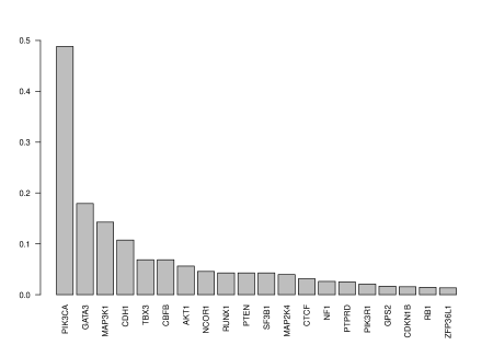
Figure 1: Mutation rates for the SMG

We calculate the mutation scores for these 20 mutations for all subjects. To assess the biological relevance of the mutation score, we study the association between the score and survival time. We consider the time to death due to disease, treating death by other causes or lost-to-followup as right censoring. The median follow-up time is 124 months, and the censoring proportion is 72.9%. For each of the 20 SMG, we classify subjects with that mutation into high-score group versus low-score group, according to whether the score is larger than or smaller than the median score for the gene among the mutated subjects; we similarly divide subjects into high-score and low-score groups for subjects without the mutation. Then, we perform the logrank test for the survival time between the high-score and low-score groups (regardless of the mutation status). To account for cancer subtypes, we also fit the Cox model of the survival time against the score status and subtype indicator. Figure 2 shows the QQ-plot for the $p$-values of the logrank tests, and Figure 3 shows the QQ-plot for the Wald test $p$-values for the score status under the Cox model.

Figure 2: QQ-plot for the logrank test $p$-values for survival VS mutation score

Figure 3: QQ-plot for the Cox $p$-values for survival VS mutation score, accounting for subtype

With or without accounting for subtype, the associations between mutation score and survival time are stronger than that expected under the null hypothesis. The results suggest that for these known important genes, the scores, as summaries of gene expressions, are associated with the survival time, and the associations remain even after accounting for subtype.

We further investigate the association between the gene score and survival time for the two most frequently mutated genes in the data set, PIK3CA and GATA3.

PIK3CA

Figure 4 shows the Kaplan–Meier curves for the high-score and low-score groups of subjects with or without a mutation in PIK3CA. In both the mutation and non-mutation groups, subjects with high scores tend to survive longer than subjects with low scores. The improvement in survival is more substantial in the mutation group (logrank $p$-value of $7.12\times 10^{-5}$) than in the non-mutation group (logrank $p$-value of 0.0110). This suggests that the gene expressions identified to be associated with the mutation of PIK3CA, as summarized by the gene score, are relevant to the survival time. Remarkably, if we compare the survival times between the mutated and non-mutated subjects, there is no significant difference between the survival functions of the two groups (logrank $p$-value $=0.739$). This suggests that the mutation status alone, without consideration of the expression of genes associated with the mutation, does not effectively distinguish subjects with different survival patterns.

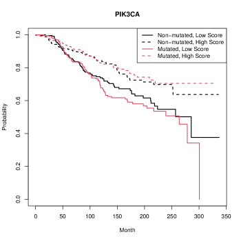
Figure 4: KM plots for subjects with different PIK3CA mutation statuses and score levels

We evaluate the association between mutation score and the mutation type. In the regression analyses, we treat a gene as mutated if it harbours any non-silent mutation within its genetic region. In the data set, the location of the mutation is actually available. Here, we classify the mutation into three groups: those located at 1047/1048, those located at 542/545, and others. Figure 5 shows the boxplot of mutation score over types of mutations and subtypes. There is no substantial difference in score between the three groups of mutation, but the difference is substantial between the two subtypes. In this case, the gene score captures the difference between the two subtypes.

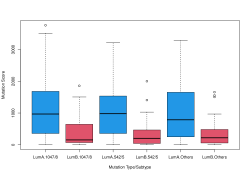
Figure 5: PIK3CA score level for subjects with different subtypes and mutation types

GATA3

For GATA3, the Kaplan–Meier curves for both mutation groups and high/low gene score groups are plotted in Figure 6. For both the mutation and non-mutation groups, subjects with high scores have overall longer survival time. The logrank test for the survival difference between the high-score and low-score groups yields a $p$-value of 0.00525. Remarkably, the two groups with no mutation and the group with mutation but low mutation score have similar survival distributions, whereas the group with mutation and high mutation score has substantially longer survival time. This suggests that it is the combination of mutation and perturbation of the associated gene expressions that drive the biological difference among the cancer patients, whereas the mutation alone may not be as effective. We perform a similar comparison of survival time but with the expression of GATA3 instead of the mutation score, and the curves are plotted in Figure 7. The group with mutation and high expression of GATA3 has longer survival than the remaining groups, but the difference between groups with high and low expression values is no longer significant under the logrank test ($p$-value $=0.178$). This suggests that the mutation score captures the biological status of the subjects better than the expression of a single gene.

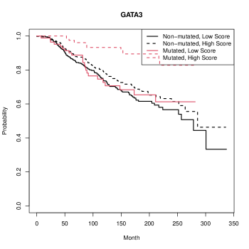
Figure 6: KM plots for subjects with different GATA3 mutation statuses and score levels

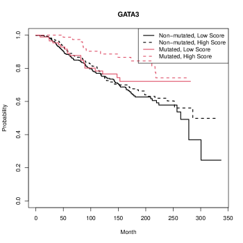
Figure 7: KM plots for subjects with different GATA3 mutation statuses and gene expression levels

We evaluate the distributions of the mutation score across different types of mutation. Following Takaku et al. (2018), we classify the mutations into three groups: the second GATA3 zinc-finger (ZnFn2) mutation, splice site mutations, and others. We present the boxplot for the mutation score across the three mutation groups and subtypes in Figure 8. We can see that for both subtypes, the scores for splice site mutations tend to be higher than the other two groups. This could explain why the combination of high score and mutation leads to change in survival time, but mutation alone may not: it is the splice site mutations that lead to difference in the survival distribution. Figure 9 shows the KM plots for subjects with different types of mutations. We can see that for both subtypes, subjects with splice site mutation tend to have the highest survival probabilities.

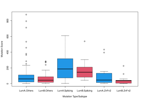
Figure 8: GATA3 score level for subjects with different subtypes and mutation types

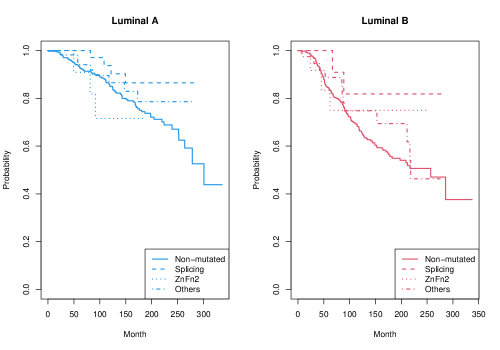
Figure 9: KM plots for subjects with different subtypes and GATA3 mutation types

5 Discussion

There are two main steps in the computation of the mutation score — model estimation and evaluation of the conditional expectation of the mutation effects. In principle, these two steps can be separated and performed on different data sets. A model can be estimated from a previous study or otherwise prespecified from prior knowledge, and then the mutation score can be computed for new subjects. Similar to DawnRank, the proposed score can be computed even for only a single subject with available mutation and gene expression data, as long as information about the association between mutation and gene expressions of the population where this subject belongs to is known.

If a gene network is not available, then the estimation of $\boldsymbol{B}$ can be replaced by a standard multivariate lasso regression, with a $(q\times p)$ unknown regression parameter matrix and a universal tuning parameter for all regression parameters. The subsequent EM algorithm and score calculation can be performed exactly as proposed. Alternatively, other penalization methods for the estimation of $\boldsymbol{B}$ that encourages group structures, such as Zhu et al. (2016), can be adopted.

The proposed method assumes that for a mutation to have effect on the expression of a gene, there must exist a directed path from the mutation to the gene in the network. To relax this assumption, we may set all mutation-to-expression effects as free parameters to be estimated and introduce another penalty for the effects that do not correspond to a path in the network.

References

- (1)
- Bashashati et al. (2012) Bashashati, A., Haffari, G., Ding, J., Ha, G., Lui, K., Rosner, J., Huntsman, D. G., Caldas, C., Aparicio, S. A., and Shah, S. P. (2012), “DriverNet: uncovering the impact of somatic driver mutations on transcriptional networks in cancer,” Genome Biology, 13, 1–14.
- Ciriello et al. (2012) Ciriello, G., Cerami, E., Sander, C., and Schultz, N. (2012), “Mutual exclusivity analysis identifies oncogenic network modules,” Genome Research, 22, 398–406.
- Curtis et al. (2012) Curtis, C., Shah, S. P., Chin, S.-F., Turashvili, G., Rueda, O. M., Dunning, M. J., Speed, D., Lynch, A. G., Samarajiwa, S., Yuan, Y. et al. (2012), “The genomic and transcriptomic architecture of 2,000 breast tumours reveals novel subgroups,” Nature, 486, 346–352.
- Friedman et al. (2010) Friedman, J., Hastie, T., and Tibshirani, R. (2010), “Regularization paths for generalized linear models via coordinate descent,” Journal of Statistical Software, 33, 1–22.
- Hou and Ma (2014) Hou, J. P., and Ma, J. (2014), “DawnRank: discovering personalized driver genes in cancer,” Genome Medicine, 6, 1–16.
- Kanehisa et al. (2012) Kanehisa, M., Goto, S., Sato, Y., Furumichi, M., and Tanabe, M. (2012), “KEGG for integration and interpretation of large-scale molecular data sets,” Nucleic Acids Research, 40, D109–D114.
- Pereira et al. (2016) Pereira, B., Chin, S.-F., Rueda, O. M., Vollan, H.-K. M., Provenzano, E., Bardwell, H. A., Pugh, M., Jones, L., Russell, R., Sammut, S.-J. et al. (2016), “The somatic mutation profiles of 2,433 breast cancers refine their genomic and transcriptomic landscapes,” Nature Communications, 7, 11479.
- Shi et al. (2016) Shi, K., Gao, L., and Wang, B. (2016), “Discovering potential cancer driver genes by an integrated network-based approach,” Molecular BioSystems, 12, 2921–2931.
- Siegel et al. (2018) Siegel, M. B., He, X., Hoadley, K. A., Hoyle, A., Pearce, J. B., Garrett, A. L., Kumar, S., Moylan, V. J., Brady, C. M., Van Swearingen, A. E. et al. (2018), “Integrated RNA and DNA sequencing reveals early drivers of metastatic breast cancer,” The Journal of Clinical Investigation, 128, 1371–1383.
- Song et al. (2019) Song, J., Peng, W., and Wang, F. (2019), “A random walk-based method to identify driver genes by integrating the subcellular localization and variation frequency into bipartite graph,” BMC Bioinformatics, 20, 1–17.
- Takaku et al. (2018) Takaku, M., Grimm, S. A., Roberts, J. D., Chrysovergis, K., Bennett, B. D., Myers, P., Perera, L., Tucker, C. J., Perou, C. M., and Wade, P. A. (2018), “GATA3 zinc finger 2 mutations reprogram the breast cancer transcriptional network,” Nature Communications, 9, 1059.
- The Cancer Genome Atlas Network (2012) The Cancer Genome Atlas Network (2012), “Comprehensive molecular portraits of human breast tumours,” Nature, 490, 61–70.
- Wang et al. (2009) Wang, H., Li, B., and Leng, C. (2009), “Shrinkage tuning parameter selection with a diverging number of parameters,” Journal of the Royal Statistical Society: Series B (Statistical Methodology), 71, 671–683.
- Wei et al. (2016) Wei, P.-J., Zhang, D., Xia, J., and Zheng, C.-H. (2016), “LNDriver: identifying driver genes by integrating mutation and expression data based on gene-gene interaction network,” BMC Bioinformatics, 17, 221–230.
- Zhu et al. (2016) Zhu, R., Zhao, Q., Zhao, H., and Ma, S. (2016), “Integrating multidimensional omics data for cancer outcome,” Biostatistics, 17, 605–618.