Trajectory Poisson multi-Bernoulli mixture filter for traffic monitoring using a drone

Abstract

This paper proposes a multi-object tracking (MOT) algorithm for traffic monitoring using a drone equipped with optical and thermal cameras. Object detections on the images are obtained using a neural network for each type of camera. The cameras are modelled as direction-of-arrival (DOA) sensors. Each DOA detection follows a von-Mises Fisher distribution, whose mean direction is obtain by projecting a vehicle position on the ground to the camera. We then use the trajectory Poisson multi-Bernoulli mixture filter (TPMBM), which is a Bayesian MOT algorithm, to optimally estimate the set of vehicle trajectories. We have also developed a parameter estimation algorithm for the measurement model. We have tested the accuracy of the resulting TPMBM filter in synthetic and experimental data sets.

I Introduction

Traffic monitoring consists of obtaining relevant information on the traffic in a given area based on sensor data [1, 2]. It provides key information that enables the improvement of the roadway system, and traffic law enforcement [3, 4]. There are different types of sensors used for traffic monitoring. For example, there are sensors that are located under or on the road: piezoelectric sensors, magnetometers, vibration sensors and loop detectors [3]. These sensors can provide valuable information on the number of vehicles and their types. However, they are difficult to install and only provide information at a given location. Other types of sensors for traffic monitoring are cameras, radars and lidars, which can be mounted next to the road or in another vehicle [3].

This paper focuses on traffic monitoring using a drone, also called an unmanned aerial vehicle [5, 6, 7]. A drone is convenient device to gather traffic data as it can be easily deployed and equipped with different sensors, such as cameras and lidars. We proceed to review the literature on traffic monitoring using drones equipped with cameras.

Traffic monitoring using a drone with cameras requires an object detection algorithm to detect vehicles on the roads and extract meaningful analytics [8]. It is also possible to improve object detection by adding road segmentation and only detect vehicles on the roads [9, 10]. In [11], several vehicle trackers on the image plane are evaluated. In [10], vehicle tracking is performed on the image plane using Kalman filters and data association methods. Velocity on the ground plane is obtained projecting the pixels to the ground plane using the ground sample distance. In [8], traffic flow estimation is performed by projecting the downward-facing image and applying the Kanade–Lucas–Tomasi (KLT) algorithm [12, 13] to estimate the background motion in low traffic. Marked geo-referenced points can also be used to accurately project pixels to the ground plane and obtain traffic statistics [6]. In [14], vehicles are detected on the image, and the optical flow using the KLT is obtained to perform the tracking. Road features are used to calculate the camera motion and pixel projection to the ground plane is achieved through an homography transformation obtained with matching points.

In this paper, we propose to use Bayesian multi-object tracking (MOT) algorithms to perform traffic monitoring directly on the ground plane. In Bayesian MOT, we require a multi-object dynamic model, which includes object births, single-object dynamics and deaths, and a multi-object measurement model [15]. We consider the standard point-object dynamic and detection-based measurement models, such that object birth follows a Poisson point process (PPP), and each object may generate at most one detection. In this framework, all information of interest about the object trajectories is included in the density of the set of (vehicle) trajectories given past and current measurements [16]. This posterior density can then be used to obtain the required traffic analytics.

The posterior density is a Poisson multi-Bernoulli mixture (PMBM) density [17, 18, 19]. The PMBM density is the union of an independent PPP and a multi-Bernoulli mixture (MBM). The PPP contains information on potential trajectories that have not yet been detected, and is useful for example in search-and-track sensor management [20]. The MBM contains the information on potential trajectories that have been detected at some point, as well as their data associations (global hypotheses). This PMBM density is computed recursively via the prediction and update steps of the trajectory PMBM (TPMBM) filter [18, 21].

Object detections from the images are obtained using a deep learning detector [22]. Then, to apply the TPMBM filter to these detections, we require a measurement model. There are several models available in the literature. In [22], the camera is modelled as a range-bearings sensor with additive Gaussian noise, with the neural network also providing depth information. In [23], the detection is converted to an azimuth measurement, which is assumed to be Gaussian distributed. In [24], the camera detection is mapped to a position with zero elevation. The measurement model is then a positional measurement on the ground plane with zero-mean Gaussian noise whose covariance matrix is calculated through the Jacobian of the projection mapping. It is also possible to use the unscented transform [25] to determine this covariance matrix [26]. The same type of approach is followed in [27] but with predefined diagonal covariance matrix for the noise.

In this paper, we model the camera as a direction-of-arrival (DOA) sensor, such that each object detection is a DOA. We use a von-Mises Fisher (VMF) distribution for DOAs, as it is a mathematically principled distribution for directional data and has benefits over Gaussian distributions for this type of data [28, 29]. For example, VMF distributions intrinsically deal with DOAs and do not require angle wrapping or external approaches to design filtering algorithms [30]. Then, using geometrical considerations, we obtain the distribution of the DOA measurement given a vehicle state, and also the distribution of the clutter measurements.

A challenge to apply the above camera-detection modelling to TPMBM filtering is to deal with the non-linear/non-Gaussian measurement updates for trajectories. One possibility is to use particle filtering techniques [31]. A computationally cheaper alternative is to use a non-linear Kalman filter, such as the extended Kalman filter (EKF) [32] or the sigma-point Kalman filters such as the unscented Kalman filter [25] and the cubature Kalman filter [32]. These filters implicitly perform a linearisation of the measurement function to obtain a Gaussian approximation to the posterior. The sigma-point Kalman filters have the following benefits over the EKF: they do not require the calculation of the Jacobian of the measurement function, and they perform the linearisation taking into account the uncertainty in the predicted density. The EKF and sigma-point Kalman filters work well for mild measurement nonlinearities [33]. However, they do not take into account the information provided by the measurement to perform the linearisation, which implies that there is room for improvement with stronger nonlinearities.

To improve performance, we therefore use the iterated posterior linearisation filter (IPLF) to perform the updates for the single-trajectory densities. The IPLF aims to obtain the best linearisation of the measurement function, as well as the resulting linearisation error, taking into account the observed measurement [34]. This property enables the IPLF to outperform the EKF and UKF if the update is sufficiently non-linear. The IPLF consists of an iterated procedure in which we linearise the measurement function in the area where the current approximation of the posterior lies. The IPLF can be implemented via sigma-points and its first iteration corresponds to a sigma-point Kalman filter update. In particular, we use the IPLF for VMF-distributed measurements and single-trajectory densities [35].

The contributions of this paper are:

• A camera measurement model, suitable for traffic monitoring with a drone, based on a deep learning detector and the VMF distribution.

• The TPMBM filter implementation with the VMF camera measurement model, the IPLF to perform the single-trajectory updates, and a suitable birth model.

• A measurement model parameter estimation algorithm based on optimising the likelihood, augmented with auxiliary variables representing data association hypotheses. The algorithm iteratively optimises the auxiliary variables, the clutter rate, probability of detection and the concentration parameter of the VMF distribution.

• The evaluation of the TPMBM filter via synthetic and experimental data using optical and thermal cameras on a Parrot Anafi USA drone [36].

The rest of the paper is organised as follows. The problem formulation is provided in Section II. In Section III, we present the multi-object measurement model. The measurement model parameter estimation algorithm is proposed in Section IV. The multi-object dynamic model is introduced in Section V. The main aspects of the Gaussian TPMBM implementation are addressed in Section VI. Finally, experimental results and conclusions are presented in Sections VII and VIII, respectively.

II System description, problem formulation, and TPMBM filtering

In this section we first describe the drone specifications in Section II-A. Then, we present the considered coordinate systems in Section II-B. We formulate the MOT problem from a Bayesian perspective in Section II-C and review the TPMBM filter in Section II-D.

II-A Drone specifications

In our experiments, we use a Parrot Anafi USA drone [36]. While the proposed algorithm is of general applicability, it is important to understand from the beginning what type of information is provided by the drone. The drone is equipped with several sensors for accurate positioning: satellite navigation (GPS, GLONASS and GALILEO), barometer, magnetometer, vertical camera and ultra-sonar, 2 inertial measurement units, 2 accelerometers and 2 gyroscopes. The drone is also equipped with two optical cameras and one thermal camera. We record video in either optical or thermal camera mode.

For each video frame, we can obtain the drone elevation, GPS location, attitude of the camera (in the form of a quaternion), and the FoV in degrees. The FoV depends on the user-defined zoom, which we assume fixed in time for simplicity. The FoV, frames per second (fps) and image size in pixels used for the optical and thermal camera modes are shown in Table I.

Table I: Video specifications

Parameter	Optical	Thermal
FoV	$\left[69^{\circ},42.27^{\circ}\right]$	$\left[46.14^{\circ},36.75^{\circ}\right]$
Fps	30	8.6
Image size	$1920\times 1080$	$1190\times 928$

II-B Coordinate systems

In this work, we use three coordinates systems: the world geodetic system (WGS) 84 format (which is the standard reference system for GPS navigation) [37], a local coordinate system for each flight, and a camera coordinate system. We proceed to explain these.

The drone coordinates in the WGS84 format, i.e., its latitude, longitude and altitude, which are obtained via satellite navigation, are recorded for each frame. For each flight, we use a local Cartesian coordinate system with the center located on the ground with the initial latitude and longitude of the drone. In this coordinate system, the $x$-axis points to the East, the $y$-axis points to the North and the $z$-axis points down. This corresponds to the initial drone north-east-down (NED) coordinate system located on the ground [37].

We also use a Cartesian coordinate system on the camera. In this coordinate system, the $x$-axis points ahead of the camera, the $y$-axis points to the right of the $x$-axis (in the direction of view), and the $z$-axis down, see Figure 1. The last two coordinate systems are used because the drone directly provides us with the rotation of this camera reference frame w.r.t. the local NED coordinate system.

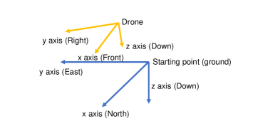
Figure 1: Cartesian coordinate systems. Local NED coordinate system with origin located on the ground and the initial latitude and longitude of the drone (blue). Camera coordinate system on the drone (yellow). The vehicles are tracked in the local coordinate system.

II-C Problem formulation

We model the MOT problem using a Bayesian approach [15]. Given the Bayesian modelling, our objective is to compute the posterior density of the set of all the vehicle trajectories (in the local coordinate system) that have been in the FoV [16]. We proceed to explain the models and the variables in the problem formulation

We make the assumption that all the objects (vehicles) are at a constant elevation in the local coordinate system. An object state in the local coordinate system is denoted by $x=\left[p_{x},v_{x},p_{y},v_{y}\right]^{T}\in\mathbb{R}^{n_{x}}$, with $n_{x}=4$, and contains its position and velocity in the local coordinate system. The set of objects at the current time step $k$ is $\mathbf{x}_{k}=\left\{x_{k}^{1},...,x_{k}^{n_{k}}\right\}$, where $n_{k}$ is the number of objects.

At each time step, each object $x\in\mathbf{x}_{k}$ can survive to the next time step with probability $p^{S}$ of survival and move with a Markovian transition density $g\left(\cdot\left|x\right.\right)$. In addition, independent new objects may be born following a PPP with intensity $\lambda_{k}^{B}\left(\cdot\right)$. According to this model, a vehicle trajectory can be represented as a variable $X=\left(t,x^{1:\nu}\right)$, where $t$ is the birth time step, $\nu$ is the trajectory length and $x^{1:\nu}=\left(x^{1},...,x^{\nu}\right)$ denotes the sequence of length $\nu$ with the object states at consecutive time steps [16]. The set of all trajectories ever present in the FoV up to the current time step $k$ is then $\mathbf{X}_{k}=\left\{X_{k}^{1},...,X_{k}^{n_{k}^{t}}\right\}$, where $n_{k}^{t}$ is the number of trajectories.

At each time step, each object $x\in\mathbf{x}_{k}$ may be detected with a probability $p^{D}$ and generate a measurement $z\in\mathbb{R}^{n_{z}}$ with density $l\left(\cdot|\mathbf{x}_{k}\right)$. The set of measurements $\mathbf{z}_{k}$ includes object-detected measurements and clutter measurements, which are distributed following a PPP with intensity $\lambda^{C}\left(\cdot\right)$.

II-D TPMBM filtering

Using the Bayesian prediction and update steps [15], we can calculate the posterior and predicted densities of $\mathbf{X}_{k^{\prime}}$, denoted by $f_{k^{\prime}|k}\left(\cdot\right)$ with $k^{\prime}\in\left\{k,k+1\right\}$, given the measurements up to time step $k$. These densities can be calculated by the TPMBM filtering recursion and are PMBMs of the form [18]

$$f_{k^{\prime}|k}\left(\mathbf{X}_{k^{\prime}}\right) =\sum_{\mathbf{Y}\uplus\mathbf{W}=\mathbf{X}_{k^{\prime}}}f_{k^{\prime}|k}^{p}\left(\mathbf{Y}\right)f_{k^{\prime}|k}^{mbm}\left(\mathbf{W}\right),$$ (1)

$$f_{k^{\prime}|k}^{p}\left(\mathbf{X}_{k^{\prime}}\right) =e^{-\int\lambda_{k^{\prime}|k}\left(X\right)dX}\left[\lambda_{k^{\prime}|k}\left(\cdot\right)\right]^{\mathbf{X}_{k^{\prime}}},$$ (2)

$$f_{k^{\prime}|k}^{mbm}\left(\mathbf{X}_{k^{\prime}}\right) =\sum_{a\in\mathcal{A}_{k^{\prime}|k}}w_{k^{\prime}|k}^{a}\sum_{\uplus_{l=1}^{n_{k^{\prime}|k}}\mathbf{X}^{l}=\mathbf{X}_{k^{\prime}}}\prod_{i=1}^{n_{k^{\prime}|k}}f_{k^{\prime}|k}^{i,a^{i}}\left(\mathbf{X}^{i}\right),$$ (3)

where (1) is the convolution formula for independent random finite sets, where we sum over all disjoint and possibly empty sets $\mathbf{Y}$ and $\mathbf{W}$ such that $\mathbf{Y}\cup\mathbf{W}=\mathbf{X}_{k^{\prime}}$ [15]. That is, (1) represents the union of an independent PPP $f_{k^{\prime}|k}^{p}\left(\cdot\right)$ with intensity $\lambda_{k^{\prime}|k}\left(\cdot\right)$, representing trajectories that remain undetected, and an MBM $f_{k^{\prime}|k}^{mbm}\left(\cdot\right)$, representing trajectories that have been detected at some point. The multi-object exponential, used in (2), is defined as $h^{\mathbf{X}}=\prod_{X\in\mathbf{X}}h\left(X\right)$ where $h$ is a real-valued function and $h^{\emptyset}=1$ by convention.

Equation (3) sums over all global data association hypotheses $a\in\mathcal{A}_{k^{\prime}|k}$, which are data-to-data hypotheses and have weight $w_{k^{\prime}|k}^{a}$. Each global hypothesis has an associated multi-Bernoulli with $n_{k^{\prime}|k}$ Bernoulli densities. Also, $a=\left(a^{1},...,a^{n_{k^{\prime}|k}}\right)$, where $a^{i}\in\left\{1,...,h^{i}\right\}$ is the index to the local hypothesis for the $i$-th Bernoulli and $h^{i}$ is the number of local hypotheses. The $i$-th Bernoulli with local hypothesis $a^{i}$ has a density

$$f_{k^{\prime}|k}^{i,a^{i}}\left(\mathbf{X}\right) =\begin{cases}1-r_{k^{\prime}|k}^{i,a^{i}}&\mathbf{X}=\emptyset\\ r_{k^{\prime}|k}^{i,a^{i}}p_{k^{\prime}|k}^{i,a^{i}}\left(X\right)&\mathbf{X}=\left\{X\right\}\\ 0&\mathrm{otherwise},\end{cases}$$ (4)

where $r_{k^{\prime}|k}^{i,a^{i}}$ is the probability of existence and $p_{k^{\prime}|k}^{i,a^{i}}\left(\cdot\right)$ its single-trajectory density, representing the trajectory information for this local hypothesis.

A detailed description of (1)-(4) and the TPMBM filtering recursion can be found in [18, 21]. To apply TPMBM filtering to drone traffic monitoring, we need to formulate the task using the models in Section II-C, which we proceed to do in the following sections.

III DOA multi-object measurement model

In this section, we present the multi-object measurement model characterising a camera as a DOA sensor. We first review the VMF distribution in Section III-A. Then, we explain the relation between a pixel and a DOA in Section III-B. We then provide the object-generated measurement model and the clutter model in Sections III-C and III-D. The overall measurement model is explained in Section III-E.

III-A Von Mises-Fisher distribution

The VMF distribution is a convenient and mathematically principled distribution for DOAs [28]. As we deal with a 3-D model, a DOA measurement is represented as a unit vector $z$ corresponding to a point in the sphere $S^{2}=\left\{z:\>z^{T}z=1,\,z\in\mathbb{R}^{3}\right\}$. The VMF distribution is unimodal and parameterised by a mean direction $\mu$ and a concentration parameter $\kappa$. Its density with respect to the uniform distribution is [28, Eq. (9.3.4)]

$$\mathcal{V}\left(z;\mu,\kappa\right) =\frac{\left(\frac{\kappa}{2}\right)^{1/2}}{\Gamma\left(3/2\right)\mathrm{I}_{1/2}\left(\kappa\right)}\exp\left(\kappa\mu^{T}z\right)\chi_{\left\|z\right\|=1}\left(z\right),$$ (5)

where $\kappa\geq 0$, $\left\|\mu\right\|=1$, $\mathrm{I}_{a}\left(\cdot\right)$ is the modified Bessel function of the first kind and order $a$, $\Gamma\left(\cdot\right)$ is the gamma function and $\chi_{A}\left(\cdot\right)$ is the indicator function on set $A$.

III-B From pixel to DOA

In this section, we explain how to convert a pixel $\left(i_{x},i_{y}\right)$ in the image to a DOA $z$ in the camera reference frame. The known camera parameters are the FoV $\left[f_{x},f_{y}\right]$ in radians, width $w$ in pixels and height $h$ in pixels. As $w$ and $h$ are even numbers, see Table I, the center pixel of the image is

$$\left(c_{x},c_{y}\right) =\left(\frac{w}{2},\frac{h}{2}\right).$$ (6)

We will test two methods to convert a pixel $\left(i_{x},i_{y}\right)$ into azimuth $\varphi\in\left[0,2\pi\right)$ and elevation $\theta\in\left[-\pi/2,\pi/2\right]$ in the camera reference frame. The first approach is to estimate $\left(\varphi,\theta\right)$ as [24, 23]

$$\varphi=\frac{i_{x}-c_{x}}{w}f_{x},\quad\theta=\frac{i_{y}-c_{y}}{h}f_{y}.$$ (7)

The second approach makes use of the pinhole camera model [38] to obtain

$$\varphi=\arctan\frac{i_{x}-c_{x}}{f_{I}},\quad\theta=\arctan\frac{i_{y}-c_{y}}{f_{I}},$$ (8)

where $f_{I}$ is the distance (in pixels) from the camera center to the image plane, which can be estimated as

$$f_{I} =\frac{1}{2}\left(\frac{w}{2\tan\left(f_{x}/2\right)}+\frac{h}{2\tan\left(f_{y}/2\right)}\right).$$ (9)

The proof of (8) and (9), and the relation with (7), is provided in Appendix A.

Using the spherical coordinates, the DOA unit vector corresponding to $\left(\varphi,\theta\right)$ is $z=\left[z_{x},z_{y},z_{z}\right]^{T}$ with [39]

$$z_{x} =\cos\varphi\cos\theta,$$ (10)

$$z_{y} =\sin\varphi\cos\theta,$$ (11)

$$z_{z} =\sin\theta.$$ (12)

III-C Single-object measurement density

The single-object measurement density $l\left(\cdot|x\right)$ given an object state $x$ is modelled as VMF (5) with

$$l\left(z|x\right) =\mathcal{V}\left(z;h(x),\kappa\right),$$ (13)

where $h(x)$ is the function that gives the mean direction for an object with state $x$. Function $h(x)$ depends on the object position $p=\left[p_{x},p_{y},0\right]^{T}\in\mathbb{R}^{3}$ in the local coordinate system, the drone location $s\in\mathbb{R}^{3}$ in the local coordinate system, and the camera frame quaternion $q=q_{1}+q_{2}i+q_{3}j+q_{4}k$, which indicates the orientation of the camera in the local coordinate system. For simplicity, we keep the dependence of $h(x)$ on $s$ and $q$ in the notation implicit.

Assuming that the drone is a point object, we obtain

$$h(x) =\frac{R_{q}\left(p-s\right)}{\left\|R_{q}\left(p-s\right)\right\|},$$ (14)

where $R_{q}$ is the rotation matrix of $q$ [40, pp. 178]

$$R_{q} =\left(\begin{array}[]{ccc}2q_{1}^{2}-1+2q_{2}^{2}&2q_{2}q_{3}+2q_{1}q_{4}&2q_{2}q_{4}-2q_{1}q_{3}\\ 2q_{2}q_{3}-2q_{1}q_{4}&2q_{1}^{2}-1+2q_{3}^{2}&2q_{3}q_{4}+2q_{1}q_{2}\\ 2q_{2}q_{4}+2q_{1}q_{3}&2q_{3}q_{4}-2q_{1}q_{2}&2q_{1}^{2}-1+2q_{4}^{2}\end{array}\right).$$ (18)

The numerator in (14) corresponds to the object position in the camera coordinate system, so $h(x)$ is the projection of this vector on the unit sphere.

III-D Clutter intensity

We model the clutter intensity as uniformly distributed in the camera FoV. In addition, the average number of clutter measurements is $\overline{\lambda}^{C}$. As the VMF density (5) is defined w.r.t. the uniform distribution, the clutter intensity must be defined w.r.t. the uniform distribution on the sphere.

Defining $\varphi\left(z\right)$ and $\theta\left(z\right)$ to be the azimuth and elevation of a measurement $z$, see (10)-(12), the camera FoV is $\mathbb{F}=\left\{z:\left\|z\right\|=1,\varphi\left(z\right)\in f_{x}/2\cdot\left[-1,1\right],\theta\left(z\right)\in f_{y}/2\cdot\left[-1,1\right]\right\}$. Then, the clutter intensity is

$$\lambda^{C}\left(z\right) =\frac{\overline{\lambda}^{C}}{u^{C}}\chi_{z\in\mathbb{F}}\left(z\right),$$ (19)

$$u^{C} =\frac{f_{x}\sin\left(f_{y}/2\right)}{2\pi},$$ (20)

where $u^{C}$ is the normalising constant of the uniform distribution on the FoV. The proof of (20) is provided in Appendix B. It should be noted that if the FoV were the whole sphere ($f_{x}=2\pi$, $f_{y}=\pi),$ then $u^{C}=1$, as the density is defined w.r.t. the uniform distribution.

III-E Multi-object measurement model

Given an image, we use a neural network to obtain a set of bounding boxes with the object detections [41]. We refer to this neural network as the object detection network. We then obtain the DOAs of the center of the bounding boxes to form the set $\mathbf{z}_{k}$ of measurements. That is, given the bounding box parameterisation $\left[b_{x},b_{y},b_{w},b_{h}\right]^{T}$, where $\left[b_{x},b_{y}\right]^{T}$ is its upper left corner, $b_{w}$ its width, and $b_{h}$ its height, the center $\left[b_{c,x},b_{c,y}\right]^{T}$ is

$$b_{c,x}=b_{x}+b_{w}/2,\quad b_{c,y}=b_{y}+b_{h}/2,$$ (21)

which can be converted to a DOA, see Section III-B.

We then assume that these object-generated DOA measurements follow the VMF distribution (13), clutter has intensity (19) and the probability of detection is a constant. With this measurement model, we can now perform the TPMBM update step from the drone images. How to select the parameters of this measurement model is explained in Section IV.

IV Measurement model parameter estimation

Once we have trained the neural network detector, we estimate the measurement model parameters $p^{D}$, $\kappa$, and $\overline{\lambda}^{C}$. To do so, we propose a coordinate ascent method [42] to maximise the likelihood after we introduce auxiliary variables that represent the data associations. We present the form of the likelihood in Section IV-A. The optimisations over the auxiliary variables and measurement model parameters are provided in Sections IV-B and IV-C, respectively.

IV-A Likelihood

For each frame $k=1,...,K$, we know the sets of DOAs $\mathbf{y}_{k}=\left\{h\left(x_{k}^{1}\right),...,h\left(x_{k}^{n_{k}}\right)\right\}$, where $\mathbf{x}_{k}=\left\{x_{k}^{1},...,x_{k}^{n_{k}}\right\}$ is the set of ground truth objects. Set $\mathbf{y}_{k}$ is obtained by mapping the center pixel of each manually annotated bounding box to a DOA, see Section III-B. We also know the set of measurements $\mathbf{z}_{k}=\left\{z_{k}^{1},...,z_{k}^{m_{k}}\right\}$ obtained by a neural network.

By applying the convolution formula [15], the likelihood of $\mathbf{z}_{k}$ given $\mathbf{x}_{k}$ is Poisson multi-Bernoulli [17]. That is, $\mathbf{z}_{k}$ is the union of independent PPP clutter and $n_{k}$ possible object-generated measurements. The density is

$$p\left(\mathbf{z}_{k}|\mathbf{x}_{k}\right) =e^{-\overline{\lambda}^{C}}\sum_{\mathbf{z}_{k}^{0}\uplus...\uplus\mathbf{z}_{k}^{n_{k}}=\mathbf{z}_{k}}\left[\prod_{z\in\mathbf{z}_{k}^{0}}\lambda^{C}\left(z\right)\right]\prod_{i=1}^{n_{k}}t\left(\mathbf{z}_{k}^{i}|x_{k}^{i}\right),$$ (22)

where the Bernoulli density of the object-generated measurements is

$$t\left(\mathbf{z}_{k}^{i}|x_{k}^{i}\right) =\begin{cases}p^{D}l(z|x_{k}^{i})&\mathbf{z}_{k}^{i}=\{z\}\\ 1-p^{D}&\mathbf{z}_{k}^{i}=\emptyset\\ 0&\mathrm{otherwise}.\end{cases}$$ (23)

In (22), the sum goes through all disjoint, and possibly empty, sets $\mathbf{z}_{k}^{0}$,…,$\mathbf{z}_{k}^{n_{k}}$ such that their union is $\mathbf{z}_{k}$.

To make parameter optimisation easier, we remove the convolution sum in (22) by the introduction of auxiliary variables. An auxiliary variable $a_{k}^{j}\in\mathbb{\mathbb{A}}_{k}=\left\{0,1,...,n_{k}\right\}$ for each measurement $z_{k}^{j}$ is defined such that an extended measurement is $\widetilde{z}_{k}^{j}=\left(a_{k}^{j},z_{k}^{j}\right)\in\mathbb{\mathbb{A}}_{k}\times S^{2}$, and $a_{k}^{j}=0$ if it is a clutter measurement and $a_{k}^{j}=i$ if it is a measurement generated by $x_{k}^{i}$ [21, 43].

Given a set of measurements with auxiliary variables $\widetilde{\mathbf{z}}_{k}$, we denote its subsets with each auxiliary variable by $\widetilde{\mathbf{z}}_{k}^{0},...,\widetilde{\mathbf{z}}_{k}^{n_{k}}$. Then, the likelihood with auxiliary variables becomes

$$\widetilde{p}\left(\widetilde{\mathbf{z}}_{k}|\mathbf{x}_{k}\right) =e^{-\overline{\lambda}^{C}}\left[\prod_{\left(0,z\right)\in\widetilde{\mathbf{z}}_{k}^{0}}\lambda^{C}\left(z\right)\right]\prod_{i=1}^{n_{k}}\widetilde{t}^{i}\left(\widetilde{\mathbf{z}}_{k}^{i}|x_{k}^{i}\right),$$ (24)

$$\widetilde{t}^{i}\left(\widetilde{\mathbf{z}}_{k}^{i}|x_{k}^{i}\right) =\begin{cases}p^{D}l(z|x_{k}^{i})&\widetilde{\mathbf{z}}_{k}^{i}=\{\left(i,z\right)\}\\ 1-p^{D}&\widetilde{\mathbf{z}}_{k}^{i}=\emptyset\\ 0&\mathrm{otherwise}.\end{cases}$$ (25)

Integrating out the auxiliary variables in (24), we obtain (22). It should be noted that the likelihood with auxiliary variables (24) is a lower bound of the likelihood (22), as all terms in (22) are positive and (24) only contains one of them. It should be noted that to evaluate (26), it is sufficient to know the set $\mathbf{y}_{k}$ of DOAs instead of $\mathbf{x}_{k}$.

Assuming that all measurements are within the FoV, the likelihood for all time steps is

$$\widetilde{p}\left(\widetilde{\mathbf{z}}_{1:K}|\mathbf{x}_{1:K}\right) =e^{-K\overline{\lambda}^{C}}\prod_{k=1}^{K}\left[\left(\frac{\overline{\lambda}^{C}}{u^{C}}\right)^{|\widetilde{\mathbf{z}}_{k}^{0}|}\prod_{i=1}^{n_{k}}t^{i}\left(\widetilde{\mathbf{z}}_{k}^{i}|x_{k}^{i}\right)\right]$$ (26)

where $\widetilde{\mathbf{z}}_{1:K}=\left(\widetilde{\mathbf{z}}_{1},...,\widetilde{\mathbf{z}}_{K}\right)$ and $\mathbf{x}_{1:K}=\left(\mathbf{x}_{1},...,\mathbf{x}_{K}\right)$.

We proceed to iteratively optimise (26) over the variables $a_{k}=\left(a_{k}^{1},...,a_{k}^{m_{k}}\right)$, $\overline{\lambda}^{C}$, $p_{D}$ and $\kappa$.

IV-B Optimising $a_{k}$

Fixing $\overline{\lambda}^{C}$, $p_{D}$ and $\kappa$, we seek the values of $a_{k}$ for $k=1,...,K$ that maximise (26). The solution can be found by solving an independent optimal assignment problem at each time step.

For time step $k$, we create an $m_{k}\times\left(n_{k}+m_{k}\right)$ cost matrix $C_{k}$ with value

$$-\ln\left(\begin{array}[]{cccccc}\frac{p^{D}l(z_{k}^{1}|x_{k}^{1})}{1-p^{D}}&...&\frac{p^{D}l(z_{k}^{1}|x_{k}^{n_{k}})}{1-p^{D}}&\frac{\overline{\lambda}^{C}}{u^{C}}&0&0\\ \vdots&\vdots&\vdots&0&\vdots&0\\ \frac{p^{D}l(z_{k}^{m_{k}}|x_{k}^{1})}{1-p^{D}}&...&\frac{p^{D}l(z_{k}^{m_{k}}|x_{k}^{n_{k}})}{1-p^{D}}&0&0&\frac{\overline{\lambda}^{C}}{u^{C}}\end{array}\right).$$ (30)

The optimal assignment can be written as an $m_{k}\times\left(n_{k}+m_{k}\right)$ binary matrix $S_{k}$ whose rows sum to one and its columns to either zero or one. Then, we can obtain the optimal assignment by minimising $\mathrm{tr}\left(S_{k}^{T}C_{k}\right)$ using the Hungarian algorithm [44] or alternative methods [45]. The optimal value of $S_{k}$ can then be written as an auxiliary variable $a_{k}$.

IV-C Optimising $\overline{\lambda}^{C}$, $p^{D}$ and $\kappa$

The optimisation over $\overline{\lambda}^{C}$, $p^{D}$ and $\kappa$ is provided in the following lemma.

Lemma 1.

Given the auxiliary variables $a_{k}$, $k=1,...,K$, the values of $\overline{\lambda}^{C}$, $p^{D}$ and $\kappa$ that maximise the likelihood (26) are

$$\overline{\lambda}^{C} =\frac{\sum_{k=1}^{K}|\mathbf{\widetilde{z}}_{k}^{0}|}{K},$$ (31)

$$p^{D} =\frac{\sum_{k=1}^{K}\sum_{i=1:\widetilde{\mathbf{z}}_{k}^{i}=\{z\}}^{n_{k}}1}{\sum_{k=1}^{K}n_{k}},$$ (32)

$$\frac{\mathrm{I}_{3/2}\left(\kappa\right)}{\mathrm{I}_{1/2}\left(\kappa\right)} =\overline{r},$$ (33)

where

$$\overline{r} =\frac{\sum_{k=1}^{K}\left[\sum_{i=1:\widetilde{\mathbf{z}}_{k}^{i}=\{z\}}^{n_{k}}\left(h\left(x_{k}^{i}\right)^{T}z\right)\right]}{\sum_{k=1}^{K}\sum_{i=1:\widetilde{\mathbf{z}}_{k}^{i}=\{z\}}^{n_{k}}1}.$$ (34)

Lemma 1 is proved in Appendix C. The optimal clutter rate (31) is the average number of clutter measurements per time step, as indicated by the auxiliary variables. Equation (32) is the empirical probability of detection for the assignments provided by the auxiliary variables. That is, the numerator is the total number of detected objects across all time steps and the denominator is the total number of objects across all time steps. Finally, $\kappa$ is obtained by solving (33), where $\overline{r}$ is a measure of the similarity of the associated DOA measurements w.r.t. $h\left(x_{k}^{i}\right)$.

For $\overline{r}\geq 0.9$, which is the case for a detector with sufficiently good performance, an accurate approximate solution to (33) is [28, Eq. (10.3.7)]

$$\kappa \simeq\frac{1}{1-\overline{r}}.$$ (35)

V Multi-object dynamic model

This section explains the multi-object dynamic model, which consists of the probability of survival $p^{S}$, the single-object transition density $g\left(\cdot\left|x\right.\right)$, and birth intensity $\lambda_{k}^{B}\left(\cdot\right)$. The models used are based on prior knowledge on the system set-up.

V-A Transition density

To model vehicle dynamics, we adopt a nearly constant velocity model [32]. The single-object transition density is

$$g\left(\cdot\left|x\right.\right) =\mathcal{N}\left(\cdot;Fx,Q\right),$$ (36)

$$F=I_{2}\otimes\left(\begin{array}[]{cc}1&\tau\\ 0&1\end{array}\right),\;Q=\sigma_{q}^{2}I_{2}\otimes\left(\begin{array}[]{cc}\tau^{3}/3&\tau^{2}/2\\ \tau^{2}/2&\tau\end{array}\right),$$ (41)

where $\tau$ is the sampling time between video frames, $F$ is the transition matrix and $Q$ the process noise covariance matrix with parameter $\sigma_{q}^{2}$, which indicates the intensity of the changes in the velocity. The probability of survival is set as a constant.

V-B Birth intensity

The birth intensity at time step $k$ is Gaussian

$$\lambda_{k}^{B}\left(x\right) =\overline{\lambda}_{k}^{B}\mathcal{N}\left(x;\overline{x}_{k}^{B},P_{k}^{B}\right),$$ (42)

where $\overline{\lambda}_{k}^{B}$ is the expected number of new born objects, $\overline{x}_{k}^{B}$ is the mean and $P_{k}^{B}$ the covariance matrix. We proceed to explain how we calculate $\overline{x}_{k}^{B}$ and $P_{k}^{B}$.

We consider that objects may appear anywhere in the FoV with a uniform angular distribution in the interval $\left[-f_{x}/2,f_{x}/2\right]\times\left[-f_{y}/2,f_{y}/2\right]$. This distribution has zero-mean and covariance

$$R^{B} =\frac{1}{12}\left(\begin{array}[]{cc}f_{x}^{2}&0\\ 0&f_{y}^{2}\end{array}\right).$$ (45)

We then map the mean and covariance of this distribution into the object positional space. To do so, we select $m$ sigma points $\mathcal{Y}_{1},...,\mathcal{Y}_{m}$ and weights $\omega_{1},...,\omega_{m}$ with zero-mean and covariance matrix using a sigma-point method [32], such as the unscented transform [25]. These points are transformed to DOAs $\mathcal{Z}_{1},...,\mathcal{Z}_{m}$ using (10)-(12), and afterwards to positional points $\mathcal{P}_{1},...,\mathcal{P}_{m}$ using the equations in Appendix D. The resulting positional mean and covariance are [32]

$$\overline{p}_{k}^{B} \approx\sum_{j=1}^{m}\omega_{j}\mathcal{P}_{j},$$ (46)

$$P_{p,k}^{B} \approx\sum_{j=1}^{m}\omega_{j}\left(\mathcal{P}_{j}-\overline{p}_{k}^{B}\right)\left(\mathcal{P}_{j}-\overline{p}_{k}^{B}\right)^{T}.$$ (47)

Then, $\overline{x}_{k}^{B}$ has the positional elements in $\overline{p}_{k}^{B}$ and zero velocity. Matrix $P_{k}^{B}$ has the positional elements in $P_{p,k}^{B}$ and the variance of the velocity elements are set to $\sigma_{v}^{2}$.

VI Gaussian TPMBM implementation

In this work, following [21, 35], we use a Gaussian implementation of the TPMBM filter for the set of all trajectories. In this setting, the single-trajectory densities $p_{k^{\prime}|k}^{i,a^{i}}\left(\cdot\right)$ in (4) have a deterministic start time and are Gaussian for each possible end time, and the PPP intensity $\lambda_{k^{\prime}|k}\left(\cdot\right)$ in (2) is a Gaussian mixture that only considers alive trajectories. We proceed to explain the main aspects of the implementation, and refer the reader to [21, 35] for all the details.

VI-A Single-trajectory density

A Gaussian density of a trajectory starting at time step $\tau$ with mean $\overline{x}$ and covariance $P$ is denoted by [21]

$$\mathcal{N}\left(t,x^{1:\nu};\tau,\overline{x},P\right) =\begin{cases}\mathcal{N}\left(x^{1:\nu};\overline{x},P\right)&t=\tau,\,\nu=\iota\\ 0&\mathrm{otherwise},\end{cases}$$ (48)

where the trajectory length is $\iota=\mathrm{dim}\left(\overline{x}\right)/n_{x}$, with $\mathrm{dim}\left(\overline{x}\right)$ being the dimensionality of vector $\overline{x}$. A trajectory with density (48) starts at time step $\tau$ and ends at time step $\tau+\iota-1$. If $k$ is the current time step, for an alive trajectory, $\tau+\iota-1=k$, and for a dead trajectory $\tau+\iota-1<k$.

In each $p_{k^{\prime}|k}^{i,a^{i}}\left(\cdot\right)$, see (4), of the Gaussian TPMBM for all trajectories [21], the birth time is known $t^{i}$, and the trajectory may end at any time between its birth and the current time step. The single-trajectory density $p_{k^{\prime}|k}^{i,a^{i}}\left(\cdot\right)$ is then of the form

$$p_{k^{\prime}|k}^{i,a^{i}}\left(X\right) =\sum_{l=t^{i}}^{k^{\prime}}\beta_{k^{\prime}|k}^{i,a^{i}}\left(l\right)\mathcal{N}\left(X;t^{i},\overline{x}_{k^{\prime}|k}^{i,a^{i}}\left(l\right),P_{k^{\prime}|k}^{i,a^{i}}\left(l\right)\right),$$ (49)

where $\beta_{k^{\prime}|k}^{i,a^{i}}\left(l\right)$ is the probability that the trajectory ends at time step $l$, and $\overline{x}_{k^{\prime}|k}^{i,a^{i}}\left(l\right)\in\mathbb{R}^{\iota n_{x}}$ and $P_{k^{\prime}|k}^{i,a^{i}}\left(l\right)\in\mathbb{R}^{\iota n_{x}\times\iota n_{x}}$, with $\iota=l-t^{i}+1$, are the mean and covariance given that the trajectory ends at time step $l$. The weights $\beta_{k^{\prime}|k}^{i,a^{i}}\left(l\right)$ sum to one over $l$.

VI-B Single-trajectory prediction and update

The multi-object dynamic model, see Section V, is linear and Gaussian, so we can directly apply the linear/Gaussian single-trajectory prediction [21]. The measurement model, see Section III, is non-linear/non-Gaussian so we need to perform a Gaussian approximation in the update. Specifically, in the update, we first perform a Gaussian approximation to the posterior of the current object state, and then we update past states of the trajectories using Gaussian properties [35, 46].

To perform the update with detection hypotheses, we use the IPLF applied to the VMF distribution [29]. In addition, we use the improvement of the normalising constant approximation explained in [47].

VI-C Practical considerations

Implementing the TPMBM filter also requires the following practical considerations. To deal with the ever increasing number of global hypotheses, we make use of ellipsoidal gating [44], Bernoulli pruning and global hypothesis pruning, in which we discard Bernoulli components with low probability of existence and global hypotheses with low weight [48]. We also use Murty’s algorithm to select global hypotheses with high weight in the update [49, 50].

As time goes on, trajectories may become increasingly long and it becomes computationally intractable to deal with the single-trajectory density (49). Therefore, we make use of the $L$-scan approximation [21], in which trajectory states before the last $L$ time steps are considered independent. This implies that the largest covariance matrices are of size $L\times L$ and the implementation can deal with long time sequences.

VII Experiments

In this section, we analyse the performance of the proposed vehicle monitoring system with synthetic and experimental data obtained with a Parrot Anafi USA drone in Liverpool. We compare different implementations of the PMBM and TPMBM filters via numerical simulations. Then, we test the accuracy of the DOA camera measurements in Section VII-B. Finally, we evaluate the filters using experimental data from the drone with optical and thermal cameras in Section VII-C.

VII-A Synthetic experiments

We compare different implementations of the PMBM and TPMBM filters in a synthetic experiment. Both filters have been implemented with the following parameters to perform the single-object updates: L0N1, L0N5 and L1N5, where L$x$N$y$ indicates that $x=1$ if there is likelihood improvement, or zero otherwise, and $y$ is the maximum number of IPLF iterations [47]. The IPLF uses the unscented transform with weight 1/3 at the origin [25] and the Kullback-Leibler divergence stopping criterion with threshold $10^{-2}$ [34, Eq. (30)]. It should be noted that the implementations with L0N1, no likelihood improvement, and 1 IPLF iteration, correspond to the UKF implementations [51], providing a baseline to assess the improvement provided by the IPLF. In turn, UKF implementations generally outperform the extended Kalman filter implementations so these are not considered [25, 33].

The filters prune Bernoulli components with existence lower than $10^{-4}$, prune MBM components with weight lower than $10^{-4}$, and prune PPP components with weight lower than $10^{-5}$. The ellipsoidal gating threshold is 50 and the maximum number of global hypothesis is 100, obtained via Murty’s algorithm [49, 50]. In addition, the TPMBM filter has been implemented with $L=1$ and $L=5$, and parameter $\Gamma_{a}=10^{-3}$ [21].

We consider a scenario, similar to [17], with 101 time steps in which 4 objects get in close proximity and then separate and one object disappears at time step 51. Objects move with $p^{S}=0.99$, $\sigma_{q}^{2}=0.5$ ($\mathrm{m^{2}/s^{3}}$) and $\tau=1/6\,\mathrm{s}$, and are born with $\overline{\lambda}_{0}^{B}=1$ and $\overline{\lambda}_{k}^{B}=0.025$ with $\sigma_{v}^{2}=20^{2}$ ($\mathrm{m}^{2}/\mathrm{s}^{2}$). The drone is located at the origin of the local coordinate system with an elevation of 25 m. The camera is pointing at point $\left(25,25,0\right)$ (m) in the local coordinate system. The VMF measurements have $\kappa=700$ and are generated using the code in [52]. The clutter intensity parameter is $\overline{\lambda}^{C}=5$.

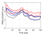
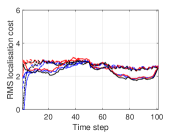
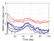
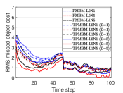
Figure 2: RMS-GOSPA error (m) and its decomposition. The TPMBM filter with $L=5$, likelihood improvement, and 5 IPLF iterations is the best performing filter.

We evaluate filter performance via Monte Carlo simulation with 100 runs. We use the generalised optimal sub-pattern assignment (GOSPA) metric with parameters $\alpha=2$, $p=2$ and $c=3\,\mathrm{m}$ to estimate the error of the ground truth set of vehicle positions and the estimated positions at each time step at the end of the simulation [53]. The root mean square GOSPA (RMS GOSPA) at each time step is shown in Figure 2. As expected, the best performing filter is TPMBM-L1N5 with $L=5$, as it uses likelihood improvement, 5 IPLF iterations and an $L$-scan window of 5. Lowering the $L$-scan window decreases performance as it does not improve estimation of past states. The PMBM has worse performance than TPMBM as it estimates object states sequentially without modifying past estimates. For the PMBM using 5 IPLF iterations and likelihood improvement also lowers the error compared to the UKF update (L0N1).

The computational times to run one Monte Carlo simulation of the algorithms on an Intel core i5 laptop are provided in Table II. The PMBM filter with L0N1 is the fastest filter. A higher number of IPLF iterations and $L$ increase the computational burden.

Table II: Computational times in seconds of the algorithms

	PMBM	TPMBM ($L=1$)	TPMBM ($L=5$)
L0N1	3.4	4.0	4.6
L0N5	5.9	9.4	10.1
L1N5	6.6	7.5	7.9

VII-B Accuracy of DOA camera measurements

In this section, we evaluate the accuracy of the estimated distances on the ground using the drone optical camera as a DOA sensor. Given a pixel on the image, we can obtain its DOA, see Section III, and then we can obtain the corresponding position on the ground, see Appendix D. Then, we can estimate distances on the ground and evaluate how accurate these estimates are. The accuracy of an estimated distance on the ground depends on several factors such as the accuracy in the drone elevation, camera quaternion, lens distortion, and gimbal stability, which depends on the drone motion and external factors such as wind speed [54].

The scenario is shown in Figure 3. The drone takes off and reaches an elevation of around 30 meters, while tilting the camera to point at the road. The length of each pavement tile measured with a tape measure is 0.9 m. We then take 5 consecutive points defined by these tiles to act as landmarks, as indicated in Figure 3.

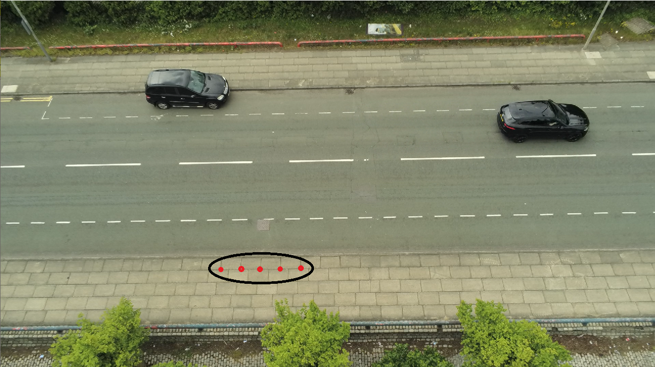
Figure 3: Image from the drone (elevation 20.8 m). The 5 points/landmarks on the pavement marked with red dots (inside the black ellipse) are used to measure the accuracy of the drone sensing system.

We identify the pixels representing the landmarks in 8 different frames of the video, with 200 frames in between these frames (which correspond to 6.7 seconds, see Table I). We have chosen these frames as they are evenly distributed while the drone is flying up and the camera is being tilted. We then calculate the distance of the corresponding points in the local coordinate system. We calculate the root mean square error (RMSE) of the estimated distances between consecutive landmarks, which are located 0.9 meters apart. We use two methods to calculate the DOA from a pixel: Method 1 uses (7) and Method 2 uses (8).

The resulting RMSEs are shown in Table III, where we also show the angles of arrival (azimuth $\varphi$ and elevation $\theta$) for the first landmark, obtained via Method 2. We can see that the RMSE stays below 0.08 m for both methods for a range of elevations and DOA. The RMSE remains unchanged from the 8-th frame on Table III until the end of the video (5.8 seconds after the 8-th frame). Across all frames, Method 2 generally performs better than Method 1 and is therefore the method we use in the next section.

Table III: RMSE of the distances between consecutive landmarks

Frame	Elevation (m)	$\varphi\,({}^{\circ})$	$\theta\,({}^{\circ})$	RMSE Method 1 (m)	RMSE Method 2 (m)
1	11.0	-7.8	3.7	0.07	0.05
2	17.1	-6.5	7.6	0.03	0.08
3	20.6	-5.5	9.3	0.06	0.06
4	20.6	-10.4	10.2	0.08	0.03
5	23.7	-9.5	8.2	0.07	0.03
6	26.8	-10.2	6.5	0.07	0.03
7	29.4	-9.4	9.6	0.08	0.03
8	31.5	-9.3	8.4	0.07	0.04

VII-C Experimental MOT performance

In this section, we analyse the performance of the proposed PMBM and TPMBM filters using recorded videos with the drone. The PMBM and TPMBM filters have also been implemented with the linear and Gaussian (LG) measurement likelihood used in [24], which uses (7). With the LG measurement likelihood, we perform a linear and Gaussian update by projecting the measurement on the ground plane. The measurement noise covariance matrix is obtained using the unscented transform with a standard deviation for the pixels of 30 [26]. We have also implemented a probability hypothesis density (PHD) filter and a cardinality PHD (CPHD) filter on the image plane [13, 15] based on the neural network detections. The estimated outputs of these filters are then projected to the ground plane, providing two additional baseline algorithms for comparison. The PHD/CPHD filters use a 4-D state vector with the position and velocity on the image plane. For the PHD/CPHD filters, the measurement noise covariance matrix is $9I_{2}$, where $I_{n}$ is the identity matrix of size $n$, and the transition density is (36) with $\sigma_{q}^{2}=9\,(\mathrm{pixel^{2}/s^{3}})$. The PHD/CPHD birth model is Gaussian with the mean at the center of the image and covariance matrix $P_{p}^{B}=\mathrm{diag}\left(\left[w^{2}/4,1,h^{2}/4,1\right]\right)$.

For each frame in the video, we have manually annotated the bounding box for each object. The available labelled data does not contain the sequence of bounding boxes of each object across all frames, which would be required to train a deep learning MOT algorithm [55, 56]. The considered multi-object dynamic model is the same as in Section VII-A but with $\tau=1/30\,\mathrm{s}$ for the optical camera and $\tau=1/8.6\,\mathrm{s}$ for the thermal camera, see Table I.

The ground truth set of object positions at each time step is considered to be the mapping of the center of each annotated bounding box in each frame to the ground plane, using (8) and Appendix D. Then, after we have processed all frames with the filters, we estimate the set of trajectories and evaluate positional errors. To do so, we compute the GOSPA metric $d_{G}\left(\cdot,\cdot\right)$ with parameters $\alpha=2$, $p=2$ and $c=3$ m at each time step, and then compute the following RMS GOSPA error across all time steps

$$d\left(\mathbf{x}_{1:K},\hat{\mathbf{x}}_{1:K}\right) =\sqrt{\frac{1}{K}\sum_{k=1}^{K}d_{G}^{2}\left(\mathbf{x}_{k},\hat{\mathbf{x}}_{k}\right)},$$ (50)

where $\mathbf{x}_{k}$ is the ground truth set of targets at time step $k$, and $\hat{\mathbf{x}}_{k}$ is its estimate. It should be noted that (50) corresponds to the metric for sets of trajectories in [57], with the track switching cost tending to zero, and normalised by the time window. The metric in [57] could only be computed explicitly if we had manually annotated the ground truth set of trajectories. Nevertheless, in traffic monitoring, objects tend to follow the road in an orderly fashion so a low number of track switches are expected in most situations. Therefore, in these scenarios, (50) provides an accurate approximation of the trajectory metric [57], even though there is no ground truth trajectory data. For example, in the synthetic experiments in Section II, the difference between the RMS trajectory metric error (with switching cost $\gamma=1$) is roughly 0.02 higher than (50) for all filters, without affecting the ranking of the algorithms.

In the rest of the subsection, we first explain the object detection network and then present the results with the optical and thermal cameras.

VII-C1 Object detection network

Any object detection network can be used in combination with our algorithm. In this experimental validation, we use a YOLOv4-tiny detector [58] due to its speed for real-time object detection and accuracy. The network only considers one object class “Vehicle”. We have manually annotated the bounding boxes of the considered videos using the Matlab Video Labeler app, helping the process with the integrated KLT point tracker algorithm [12]. We have used 6 optical camera videos and 6 thermal videos, all obtained in daylight conditions. The lengths of the videos and the ranges of drone elevations are provided in Table IV.

Table IV: Length and range of drone elevations of the videos

	Optical		Thermal
Video	Length (s)	Elevation (m)	Length (s)	Elevation (m)
1	23	34 - 34	12	29 - 30
2	109	14 - 35	30	30 - 31
3	98	28 - 40	43	41 - 45
4	96	35 - 35	39	35 - 36
5	50	40 - 40	69	40 - 40
6	32	36 - 36	45	31 - 31

The training of the detector for optical images has been performed by re-training a pre-trained model on the COCO data set. Re-training has been performed with 3 videos. We have used an input size of $416\times 416\times 3$ and 6 anchor boxes, whose sizes are estimated from the training data [59]. We have used data augmentation with random horizontal flipping, color jittering, X/Y scaling, and rotations from $-90^{\circ}$ to $90^{\circ}$. The optimisation algorithm is the Adam optimiser, with initial learning rate 0.001, mini-batch size of 8, moving batch normalisation statistics, and a maximum number of epochs of 200. For the thermal images, we have re-trained the obtained detector for optical images using 3 thermal videos. We have performed this re-training as the features of the vehicles on both type of images are quite similar.

In addition, for each video frame, we have also extracted the latitude, longitude, elevation and camera quaternion of the drone from the video metadata using ExifTool. These are required to establish the coordinate systems, see Section II-B, and run the filters.

VII-C2 Optical camera

We use video 4 to perform the measurement model parameter estimation, see Section IV. The resulting parameters are $p^{D}=0.95$, $\kappa=65000$, and $\overline{\lambda}^{C}=0.05$. The RMS GOSPA errors (50) for the algorithms are provided in Table V. We can see that the TPMBM ($L=5$) with 5 IPLF iterations and likelihood improvement is the best performing filter in general. This result is to be expected as it is the filter with highest performance in theory, and can improve the estimation of past states of the trajectories. The PMBM filter implementations with L1N5 generally have worse performance than the TPMBM implementations. Overall, the proposed PMBM and TPMBM filter implementations outperform the LG implementations and the PHD/CPHD filters on the image plane.

Table V: RMS GOSPA errors across time in the optical videos

	PHD	CPHD	PMBM				TPMBM ($L=1$)				TPMBM ($L=5$)
Video	-	-	LG	L0N1	L0N5	L1N5	LG	L0N1	L0N5	L1N5	LG	L0N1	L0N5	L1N5
1	1.38	1.44	1.70	1.92	0.82	0.87	1.66	2.18	0.79	0.79	1.63	2.02	0.77	0.78
2	1.46	1.47	2.31	1.06	0.92	0.89	2.32	1.19	0.90	0.89	2.27	1.12	0.86	0.86
3	1.44	1.28	4.48	0.70	0.73	0.73	4.48	0.76	0.70	0.70	4.47	0.69	0.69	0.69
4	1.38	1.39	2.23	1.10	0.86	0.83	2.23	1.21	0.85	0.85	2.19	1.16	0.83	0.82
5	2.40	2.46	3.01	1.92	1.97	1.92	3.01	1.97	1.90	1.88	2.98	1.90	1.88	1.86
6	3.17	3.20	4.16	2.88	2.87	2.82	4.16	2.90	2.83	2.82	4.11	2.80	2.79	2.79

VII-C3 Thermal camera

An example of a thermal image from the drone is shown in Figure 4. Using thermal video 4, the measurement model parameter estimation algorithm provides $p^{D}=0.99$ $\kappa=58800$, and $\overline{\lambda}^{C}=0.07$. The RMS GOSPA errors (50) for the algorithms are provided in Table VI. As with the optical camera, the TPMBM filter is the best performing filter. The TPMBM implementation with $L=5$, likelihood improvement and 5 IPLF iterations generally provides the best estimates of the vehicle trajectories. The TPMBM with $L=1$, no likelihood improvement and 1 IPLF iteration performs slightly worse. The PMBM filter shows a decrease in performance compared to the TPMBM filter. The LG implementations and the PHD/CPHD filters on the image plane do not perform as well as the proposed implementations of the TPMBM and PMBM filters.

Figure 4: Example of a thermal image of a roundabout with 7 vehicles, one of them entering the image (elevation 44.7 m).

Table VI: RMS GOSPA errors across time in the thermal videos

	PHD	CPHD	PMBM				TPMBM ($L=1$)				TPMBM ($L=5$)
Video	-	-	LG	L0N1	L0N5	L1N5	LG	L0N1	L0N5	L1N5	LG	L0N1	L0N5	L1N5
1	1.53	1.80	1.30	0.76	0.82	0.72	1.29	0.74	0.66	0.72	1.34	0.70	0.66	0.72
2	1.72	1.97	1.39	0.82	1.05	0.81	1.36	0.77	0.73	0.66	1.35	0.73	0.72	0.65
3	2.34	2.53	2.51	1.57	1.68	1.56	2.50	1.54	1.52	1.51	2.47	1.49	1.50	1.49
4	2.31	2.51	2.06	1.75	1.78	1.74	2.04	1.71	1.68	1.68	2.06	1.68	1.67	1.67
5	1.45	1.43	0.99	0.75	0.93	0.76	0.96	0.63	0.61	0.61	1.04	0.62	0.62	0.62
6	3.23	3.24	2.88	2.82	2.96	2.82	2.86	2.80	2.80	2.79	2.89	2.80	2.79	2.78

VIII Conclusions

This paper has proposed a multi-object tracking algorithm for vehicle monitoring using a drone equipped with a camera. The camera is modelled as a DOA sensor with its uncertainty modelled as a VMF distribution. We have derived the corresponding measurement model, which requires mapping the vehicle position on the ground into a direction of arrival, making use of the drone camera pose.

The multi-object tracking algorithm is based on the PMBM filter for sets of trajectories, which provides us with the optimal Bayesian solution for trajectory estimation under the standard multi-object tracking models. To apply this detection-based filter, vehicles in the image are detected using a neural network, retrained with labelled images obtained by the drone.

We have also derived a measurement model parameter estimation algorithm that enables us to obtain the probability of detection, clutter intensity and concentration parameter that best fit a lower bound on the likelihood. This algorithm can also be used to obtain the best parameters for different conditions, such as changing illumination or weather.

The algorithm has been first tested via numerical simulations. We have also carried out an experimental validation to test the accuracy of estimated distances on the ground, and the vehicle tracking accuracy using optical and thermal cameras.

Appendix A

In this appendix, we prove (8) and (9) using the pinhole camera model [38] assuming that pixels are evenly distributed on the image plane. We also show the connection with (7). From the camera specifications, see Table I, we know the FoV along the horizontal and vertical axes ($f_{x}$ and $f_{y}$ in radians) as well as the width $w$ and height $h$ in pixels. Using the pinhole camera model and just considering $f_{x}$ and $h$ (horizontal axis), we obtain the estimate $f_{I,x}$ of $f_{I}$ as [38]

$$f_{I,x} =\frac{w}{2\tan\left(f_{x}/2\right)}.$$ (51)

Performing the same calculation for the vertical axis, we obtain $f_{I,y}$ by substituting $h$ and $f_{y}$ instead of $w$ and $f_{x}$ in the previous equation. Equation (9) is the average between $f_{I,x}$ and $f_{I,y}$.

Using the geometry of the pinhole camera model, we obtain

$$\tan\varphi= \frac{i_{x}-c_{x}}{f_{I}}.$$ (52)

The same process can be used to obtain $\theta$ and prove (8).

Considering the values in Table I, we obtain $f_{I,x}=1396.81$ and $f_{I,y}=1396.90$ for the optical camera, which are very similar values. If we use $f_{I,x}$ instead of $f_{I}$ in for $\varphi$ and $f_{I,y}$ instead of $f_{I}$ in for $\theta$ in (8), and we approximate $\tan x\approx x$, valid for sufficiently small $x$, we obtain (7).

Appendix B

In this appendix, we calculate the normalising constant $u^{C}$ of the clutter intensity, see (20). To do so, we integrate the differential spherical area element (surface element) on the unit sphere [39] in the region of the camera FoV. In addition, as the VMF density is defined w.r.t. the uniform distribution, see (5), we need to divide the previous integral by $4\pi$, which is the area of the unit sphere. That is, we have that

$$u^{C} =\frac{1}{4\pi}\int_{-f_{x}/2}^{f_{x}/2}\int_{\pi/2-f_{y}/2}^{\pi/2+f_{y}/2}\sin\theta d\varphi d\theta.$$ (53)

This integral can be solved analytically yielding (20).

Appendix C

In this appendix, we prove Lemma 1. The log likelihood can be obtained from (26), (25) and (5) as

$$L =\ln\widetilde{p}\left(\widetilde{\mathbf{z}}_{1:K}|\mathbf{x}_{1:K}\right)$$

$$=\sum_{k=1}^{K}\left[|\widetilde{\mathbf{z}}_{k}^{0}|\ln\left(\frac{\overline{\lambda}^{C}}{u^{C}}\right)+\sum_{i=1:|\widetilde{\mathbf{z}}_{k}^{i}|=\emptyset}^{n_{k}}\ln\left(1-p^{D}\right)\right.$$

$$+\sum_{i=1:\widetilde{\mathbf{z}}_{k}^{i}=\{z\}}^{n_{k}}\left(\ln p^{D}+1/2\ln\frac{\kappa}{2}+\kappa h\left(x_{k}^{i}\right)^{T}z\right.$$

$$\left.\left.-\ln\mathrm{I}_{1/2}\left(\kappa\right)-\ln\Gamma\left(3/2\right)\right)\vphantom{\ln\left(\frac{\overline{\lambda}^{C}}{u^{C}}\right)}\right]-K\overline{\lambda}^{C}.$$ (54)

We proceed to maximise (54) w.r.t. $\overline{\lambda}^{C}$, $p^{D}$ and $\kappa$ in the following subsections.

C-A Optimisation of (54) w.r.t. $\overline{\lambda}^{C}$

The derivative of (54) w.r.t. $\overline{\lambda}^{C}$ is

$$\frac{\partial L}{\partial\overline{\lambda}^{C}} =-K+\frac{1}{\overline{\lambda}^{C}}\sum_{k=1}^{K}|\mathbf{\widetilde{z}}_{k}^{0}|.$$ (55)

Equating (55) to zero, we obtain (31). Taking the second derivative, we can check (31) is a maximum.

C-B Optimisation of (54) w.r.t. $p^{D}$

The derivative of (54) w.r.t. $p^{D}$ is

$$\frac{\partial L}{\partial p_{D}} =\frac{-1}{1-p^{D}}\left[\sum_{k=1}^{K}\sum_{i=1:|\widetilde{\mathbf{z}}_{k}^{i}|=\emptyset}^{n_{k}}1\right]$$

$$+\frac{1}{p^{D}}\left[\sum_{k=1}^{K}\sum_{i=1:\widetilde{\mathbf{z}}_{k}^{i}=\{z\}}^{n_{k}}1\right].$$ (56)

Equating (56) to zero, we obtain (32). Taking the second derivative, we can check (32) is a maximum.

C-C Optimisation of (54) w.r.t. $\kappa$

The derivative of (54) w.r.t. $\kappa$ is

$$\frac{\partial L}{\partial\kappa} =\sum_{k=1}^{K}\left[\sum_{i=1:\widetilde{\mathbf{z}}_{k}^{i}=\{z\}}^{n_{k}}\left(h\left(x_{k}^{i}\right)^{T}z\right)\right]$$

$$+\left(\frac{1}{2\kappa}-\frac{\frac{\partial\mathrm{I}_{1/2}\left(\kappa\right)}{\partial\kappa}}{\mathrm{I}_{1/2}\left(\kappa\right)}\right)\sum_{k=1}^{K}\sum_{i=1:\widetilde{\mathbf{z}}_{k}^{i}=\{z\}}^{n_{k}}1.$$ (57)

Equating (57) to zero and applying the equality [28, Eq. (A.8)]

$$\frac{\partial\mathrm{I}_{1/2}\left(\kappa\right)}{\partial\kappa} =\frac{1}{2\kappa}\mathrm{I}_{1/2}\left(\kappa\right)+\mathrm{I}_{3/2}\left(\kappa\right),$$ (58)

we obtain that the stationary point for $\kappa$ meets (33). Then, considering that $\mathrm{I}_{3/2}\left(\kappa\right)/\mathrm{I}_{1/2}\left(\kappa\right)$ is a strictly increasing function [60], the second derivative is negative, which proves that the stationary point is a maximum.

Appendix D

In this appendix, given a pixel $\left(i_{x},i_{y}\right)$, we calculate the corresponding position $\left[p_{x},p_{y},0\right]^{T}$ of an object on the ground in the local coordinate system. We first obtain the DOA $z$ in the camera reference frame using (8) and (10)-(12). The DOA vector in the local coordinate system $\nu=\left[\nu_{x},\nu_{y},\nu_{z}\right]^{T}$ is calculated with the inverse rotation of (18) such that

$$\nu =\left(R_{q}\right)^{-1}z.$$ (59)

Then, given the sensor position $\left[s_{x},s_{y},s_{z}\right]^{T}$ in the local coordinate system, the point on the ground $\left[p_{x},p_{y},0\right]^{T}$ with this DOA meets

$$\left[s_{x},s_{y},s_{z}\right]^{T}+\lambda\left[\nu_{x},\nu_{y},\nu_{z}\right]^{T}=\left[p_{x},p_{y},0\right]^{T},$$ (60)

where $\lambda\in\mathbb{R}$. In (60), the left-hand side represents the line defined by the DOA.

Solving for $\lambda$ in (60) yields that the position on the ground has $(p_{x},p_{y})$ coordinates

$$p_{x}=s_{x}-\frac{s_{z}}{\nu_{z}}\nu_{x},\quad p_{y}=s_{y}-\frac{s_{z}}{\nu_{z}}\nu_{y}.$$ (61)

References

- [1] J. Zhou, D. Gao, and D. Zhang, “Moving vehicle detection for automatic traffic monitoring,” IEEE Transactions on Vehicular Technology, vol. 56, no. 1, pp. 51–59, 2007.
- [2] R. Du, C. Chen, B. Yang, N. Lu, X. Guan, and X. Shen, “Effective urban traffic monitoring by vehicular sensor networks,” IEEE Transactions on Vehicular Technology, vol. 64, no. 1, pp. 273–286, 2015.
- [3] M. Won, “Intelligent traffic monitoring systems for vehicle classification: A survey,” IEEE Access, vol. 8, pp. 73 340–73 358, 2020.
- [4] S. Pan, P. Li, C. Yi, D. Zeng, Y.-C. Liang, and G. Hu, “Edge intelligence empowered urban traffic monitoring: A network tomography perspective,” IEEE Transactions on Intelligent Transportation Systems, vol. 22, no. 4, pp. 2198–2211, 2021.
- [5] V. Vahidi, E. Saberinia, and B. T. Morris, “OFDM performance assessment for traffic surveillance in drone small cells,” IEEE Transactions on Intelligent Transportation Systems, vol. 20, no. 8, pp. 2869–2878, 2019.
- [6] E. N. Barmpounakis, E. I. Vlahogianni, J. C. Golias, and A. Babinec, “How accurate are small drones for measuring microscopic traffic parameters?” Transportation Letters, vol. 11, no. 6, pp. 332–340, 2019.
- [7] H. Huang and A. V. Savkin, “Navigating UAVs for optimal monitoring of groups of moving pedestrians or vehicles,” IEEE Transactions on Vehicular Technology, vol. 70, no. 4, pp. 3891–3896, 2021.
- [8] R. Ke, Z. Li, J. Tang, Z. Pan, and Y. Wang, “Real-time traffic flow parameter estimation from UAV video based on ensemble classifier and optical flow,” IEEE Transactions on Intelligent Transportation Systems, vol. 20, no. 1, pp. 54–64, 2019.
- [9] C. Kyrkou, S. Timotheou, P. Kolios, T. Theocharides, and C. G. Panayiotou, “Optimized vision-directed deployment of UAVs for rapid traffic monitoring,” in IEEE International Conference on Consumer Electronics, 2018, pp. 1–6.
- [10] R. Makrigiorgis, N. Hadjittoouli, C. Kyrkou, and T. Theocharides, “AirCamRTM: Enhancing vehicle detection for efficient aerial camera-based road traffic monitoring,” in IEEE/CVF Winter Conference on Applications of Computer Vision, 2022, pp. 3431–3440.
- [11] D. Du et al., “The unmanned aerial vehicle benchmark: Object detection and tracking,” in Proceedings of the European Conference on Computer Vision, pp. 370–386.
- [12] B. D. Lucas and T. Kanade, “An iterative image registration technique with an application to stereo vision,” in Proceedings of Imaging Understanding Workshop, 1981, pp. 121–130.
- [13] E. Maggio and A. Cavallaro, Video Tracking: Theory and Practice. John Wiley & Sons, 2011.
- [14] L. Wang, F. Chen, and H. Yin, “Detecting and tracking vehicles in traffic by unmanned aerial vehicles,” Automation in Construction, vol. 72, pp. 294–308, 2016.
- [15] R. P. S. Mahler, Advances in Statistical Multisource-Multitarget Information Fusion. Artech House, 2014.
- [16] A. F. García-Fernández, L. Svensson, and M. R. Morelande, “Multiple target tracking based on sets of trajectories,” IEEE Transactions on Aerospace and Electronic Systems, vol. 56, no. 3, pp. 1685–1707, Jun. 2020.
- [17] J. L. Williams, “Marginal multi-Bernoulli filters: RFS derivation of MHT, JIPDA and association-based MeMBer,” IEEE Transactions on Aerospace and Electronic Systems, vol. 51, no. 3, pp. 1664–1687, July 2015.
- [18] K. Granström, L. Svensson, Y. Xia, J. L. Williams, and A. F. García-Fernández, “Poisson multi-Bernoulli mixture trackers: continuity through random finite sets of trajectories,” in 21st International Conference on Information Fusion, 2018, pp. 973–981.
- [19] G. Li, L. Kong, W. Yi, and X. Li, “Robust Poisson multi-Bernoulli mixture filter with unknown detection probability,” IEEE Transactions on Vehicular Technology, vol. 70, no. 1, pp. 886–899, 2021.
- [20] P. Boström-Rost, D. Axehill, and G. Hendeby, “Sensor management for search and track using the Poisson multi-Bernoulli mixture filter,” IEEE Transactions on Aerospace and Electronic Systems, vol. 57, no. 5, pp. 2771–2783, 2021.
- [21] A. F. García-Fernández, L. Svensson, J. L. Williams, Y. Xia, and K. Granström, “Trajectory Poisson multi-Bernoulli filters,” IEEE Transactions on Signal Processing, vol. 68, pp. 4933–4945, 2020.
- [22] S. Scheidegger, J. Benjaminsson, E. Rosenberg, A. Krishnan, and K. Granström, “Mono-camera 3D multi-object tracking using deep learning detections and PMBM filtering,” in IEEE Intelligent Vehicles Symposium, 2018, pp. 433–440.
- [23] Ø. K. Helgesen, K. Vasstein, E. F. Brekke, and A. Stahl, “Heterogeneous multi-sensor tracking for an autonomous surface vehicle in a littoral environment,” Ocean Engineering, vol. 252, pp. 1–16, 2022.
- [24] Ø. K. Helgesen, E. F. Brekke, A. Stahl, and Ø. Engelhardtsen, “Low altitude georeferencing for imaging sensors in maritime tracking,” in 21st IFAC World Congress, vol. 53, no. 2, 2020, pp. 14 476–14 481.
- [25] S. J. Julier and J. K. Uhlmann, “Unscented filtering and nonlinear estimation,” Proceedings of the IEEE, vol. 92, no. 3, pp. 401–422, Mar. 2004.
- [26] Ø. K. Helgesen, A. Stahl, and E. F. Brekke, “Maritime tracking with georeferenced multi-camera fusion,” IEEE Access, vol. 11, pp. 30 340–30 359, 2023.
- [27] S. Sharma, J. A. Ansari, J. K. Murthy, and K. M. Krishna, “Beyond pixels: Leveraging geometry and shape cues for online multi-object tracking,” in Procedings of the IEEE International Conference on Robotics and Automation, 2018.
- [28] K. V. Mardia and P. E. Jupp, Directional Statistics. John Wiley & Sons, 2000.
- [29] A. F. García-Fernández, F. Tronarp, and S. Särkkä, “Gaussian target tracking with direction-of-arrival von Mises-Fisher measurements,” IEEE Transactions on Signal Processing, vol. 67, pp. 2960–2972, June 2019.
- [30] D. F. Crouse, “Cubature/unscented/sigma point Kalman filtering with angular measurement models,” in 18th International Conference on Information Fusion, July 2015, pp. 1550–1557.
- [31] M. Arulampalam, S. Maskell, N. Gordon, and T. Clapp, “A tutorial on particle filters for online nonlinear/non-Gaussian Bayesian tracking,” IEEE Transactions on Signal Processing, vol. 50, no. 2, pp. 174–188, Feb. 2002.
- [32] S. Särkkä, Bayesian Filtering and Smoothing. Cambridge University Press, 2013.
- [33] M. R. Morelande and A. F. García-Fernández, “Analysis of Kalman filter approximations for nonlinear measurements,” IEEE Transactions on Signal Processing, vol. 61, no. 22, pp. 5477–5484, Nov. 2013.
- [34] A. F. García-Fernández, L. Svensson, M. R. Morelande, and S. Särkkä, “Posterior linearization filter: principles and implementation using sigma points,” IEEE Transactions on Signal Processing, vol. 63, no. 20, pp. 5561–5573, Oct. 2015.
- [35] A. F. García-Fernández, J. Ralph, P. Horridge, and S. Maskell, “Gaussian trajectory PMBM filter with nonlinear measurements based on posterior linearisation,” in Proceedings of the 25th International Conference on Information Fusion, 2022, pp. 1–8.
- [36] Parrot drones, “Anafi USA white paper, v. 1.5.2,” Tech. Rep. [Online]. Available: https://www.parrot.com/uk/drones/anafi-usa
- [37] G. Cai, B. M. Chen, and T. H. Lee, Unmanned Rotorcraft Systems. Springer, 2011.
- [38] R. Hartley and A. Zisserman, Multiple View Geometry in Computer Vision. Cambridge University Press, 2003.
- [39] C. H. Edwards Jr., Advanced Calculus of Several Variables. Academic Press, Inc., 1973.
- [40] J. B. Kuipers, Quaternions and Rotation sequences: A Primer with Applications to Orbits, Aerospace and Virtual Reality. Princeton University Press, 1999.
- [41] W. Luo, J. Xing, A. Milan, X. Zhang, W. Liu, and T.-K. Kim, “Multiple object tracking: A literature review,” Artificial Intelligence, vol. 293, pp. 1–23, 2021.
- [42] J. Nocedal and S. J. Wright, Numerical Optimization. Springer, 1999.
- [43] H. Kim, K. Granstrom, L. Svensson, S. Kim, and H. Wymeersch, “PMBM-based SLAM filters in 5G mmwave vehicular networks,” IEEE Transactions on Vehicular Technology, vol. 71, no. 8, pp. 8646–8661, 2022.
- [44] S. Blackman and R. Popoli, Design and Analysis of Modern Tracking Systems. Artech House, 1999.
- [45] D. F. Crouse, “On implementing 2D rectangular assignment algorithms,” IEEE Transactions on Aerospace and Electronic Systems, vol. 52, no. 4, pp. 1679–1696, August 2016.
- [46] F. Beutler, M. F. Huber, and U. D. Hanebeck, “Gaussian filtering using state decomposition methods,” in 12th International Conference on Information Fusion, July 2009, pp. 579–586.
- [47] A. F. García-Fernández, J. Ralph, P. Horridge, and S. Maskell, “A Gaussian filtering method for multi-target tracking with nonlinear/non-Gaussian measurements,” IEEE Transactions on Aerospace and Electronic Systems, vol. 57, no. 5, pp. 3539–3548, 2021.
- [48] K. Granström, M. Fatemi, and L. Svensson, “Poisson multi-Bernoulli mixture conjugate prior for multiple extended target filtering,” IEEE Transactions on Aerospace and Electronic Systems, vol. 56, no. 1, pp. 208–225, Feb. 2020.
- [49] K. G. Murty, “An algorithm for ranking all the assignments in order of increasing cost.” Operations Research, vol. 16, no. 3, pp. 682–687, 1968.
- [50] A. F. García-Fernández, J. L. Williams, K. Granström, and L. Svensson, “Poisson multi-Bernoulli mixture filter: direct derivation and implementation,” IEEE Transactions on Aerospace and Electronic Systems, vol. 54, no. 4, pp. 1883–1901, Aug. 2018.
- [51] M. R. Morelande, “Tracking multiple targets with a sensor network,” in 9th International Conference on Information Fusion, July 2006, pp. 1–7.
- [52] Y. H. Chen, D. Wei, G. Newstadt, M. DeGraef, J. Simmons, and A. Hero, “Parameter estimation in spherical symmetry groups,” IEEE Signal Processing Letters, vol. 22, no. 8, pp. 1152–1155, Aug. 2015.
- [53] A. S. Rahmathullah, A. F. García-Fernández, and L. Svensson, “Generalized optimal sub-pattern assignment metric,” in 20th International Conference on Information Fusion, 2017, pp. 1–8.
- [54] X. Liu, Y. Yang, C. Ma, J. Li, and S. Zhang, “Real-time visual tracking of moving targets using a low-cost unmanned aerial vehicle with a 3-axis stabilized gimbal system,” Applied Sciences, vol. 10, no. 15, 2020.
- [55] Y. Xu, A. Osep, Y. Ban, R. Horaud, L. Leal-Taixé, and X. Alameda-Pineda, “How to train your deep multi-object tracker,” in IEEE/CVF Conference on Computer Vision and Pattern Recognition, 2020, pp. 6786–6795.
- [56] A. Milan, L. Leal-Taixé, I. Reid, S. Roth, and K. Schindler, “MOT16: a benchmark for multi-object tracking.” [Online]. Available: https://arxiv.org/abs/1603.00831
- [57] A. F. García-Fernández, A. S. Rahmathullah, and L. Svensson, “A metric on the space of finite sets of trajectories for evaluation of multi-target tracking algorithms,” IEEE Transactions on Signal Processing, vol. 68, pp. 3917–3928, 2020.
- [58] C.-Y. Wang, A. Bochkovskiy, and H.-Y. M. Liao, “Scaled-YOLOv4: Scaling cross stage partial network,” in Proceedings of the IEEE/CVF Conference on Computer Vision and Pattern Recognition, 2021, pp. 13 029–13 038.
- [59] J. Redmon and A. Farhadi, “YOLO9000: Better, faster, stronger,” in Proceedings of the IEEE Conference on Computer Vision and Pattern Recognition, July 2017.
- [60] G. Schou, “Estimation of the concentration parameter in von Mises-Fisher distributions,” Biometrika, vol. 65, no. 2, pp. 369–377, 1978.