The History of The Milky Way: The Evolution of Star Formation, Cosmic Rays, Metallicity, and Stellar Dynamics over Cosmic Time

Abstract

We study the long-term evolution of the Milky Way (MW) over cosmic time by modeling the star formation, cosmic rays, metallicity, stellar dynamics, outflows and inflows of the galactic system to obtain various insights into the galactic evolution. The mass accretion is modeled by the results of cosmological $N$-body simulations for the cold dark matter. We find that the star formation rate is about half the mass accretion rate of the disk, given the consistency between observed Galactic Diffuse X-ray Emissions (GDXEs) and possible conditions driving the Galactic wind. Our model simultaneously reproduces the quantities of star formation rate, cosmic rays, metals, and the rotation curve of the current MW. The most important predictions of the model are that there is an unidentified accretion flow with a possible number density of $\sim 10^{-2}~{}{\rm cm^{-3}}$ and the part of the GDXEs originates from a hot, diffuse plasma which is formed by consuming about 10 % of supernova explosion energy. The latter is the science case for future X-ray missions; XRISM, Athena, and so on. We also discuss further implications of our results for the planet formation and observations of externalgalaxies in terms of the multimessenger astronomy.

1 Introduction

The evolution of galaxies over cosmic time is related to many astrophysical subjects such as the formation of stars, the origin of cosmic rays (CRs) and radiation, and the evolution of the environment for the life on the planets, and has been widely studied (e.g., [van der Kruit & Freeman (2011), Putman et al. (2012), Naab & Ostriker (2017)]). Nevertheless, our current understanding is far from sufficient. The long-term star formation rate of the Milky Way (MW), which continues with an almost constant rate of several $M_{\odot}~{}{\rm yr^{-1}}$ throughout the cosmic age (e.g., [Haywood et al. (2016)]), is a representative puzzle; if the constant star formation resulted from the similar Galactic disk conditions during the cosmic age of $14$ Gyr, the gaseous matter with a mass of $\sim 10^{9}~{}M_{\odot}$ would have been depleted within $\sim 1$ Gyr. This puzzle can be translated by the cosmological context. Supposing the cosmic density ratio of the baryon to dark matter (DM), $\sim 0.1$ ([Planck Collaboration et al. (2020)]), the total baryon mass of the MW is estimated to be $\sim 10^{11}~{}M_{\odot}$, while the total mass of stars is $4\mathchar 45\relax 6\times 10^{10}~{}M_{\odot}$ ([Bland-Hawthorn & Gerhard (2016)]). Therefore, we need to find an explanation why the half of the gaseous matter is converted into the stars, leaving $\sim 1$ % of the mass in the galactic disk. In this paper, we construct the galactic evolution model to elucidate what can be the essence of this fine-tuning mechanism.

The galactic wind (outflow from the disk) is invoked to explain the observed metal absorption lines in the circumgalactic medium (CGM, [Tumlinson et al. (2017)]). Shimoda & Inutsuka (2022) studied the galactic wind considering the effects of the radiative cooling and CR diffusion for the case of the MW. They found that the current conditions of the MW allow the existence of the wind with a mass transfer rate of several $M_{\odot}~{}{\rm yr}^{-1}$ which is comparable to the star formation rate. Thus, the galactic wind is also important for the mass budget of the Galactic system. They also pointed out that the mass loss due to the wind and star formation should be balanced with the disk mass accretion to explain the constant star formation rate over cosmic time. In this paper, following their considerations, we dedicate to find the possible gas accretion to reproduce the current conditions of the MW.

Since we consider the CR-driven wind and the metal-polluted CGM, our model also predicts the amounts of CRs and metals, simultaneously. The combination of predictions on the star formation, the CRs, the metals, and the gaseous matter distribution can be useful for the broad astrophysical subjects such as the planet formation (e.g., Tsukamoto & Okuzumi (2022); Tsukamoto et al. (2022)) and particle astrophysics in terms of the multimessenger astronomy (e.g., Murase (2022)). Therefore, the implications for various observations are important to test our model. These are also discussed in this paper.

This paper is organized as follows: In section 2, we review the important physical processes through the construction of our model and present analytical estimates of the current star formation rate, metallicity, and CR energy density. The numerical results of our model are presented in section 3. We discuss the implications for observations and future prospects in section 4 and summarize our results in section 5. We will find that the origins of the outflow and inflow are controversially uncertain, although they are really important for understanding galactic evolution.

2 Model Description

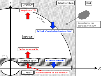
Figure 1: Schematic illustration of our model. The horizontal axis shows the radial distance $R$ in cylindrical coordinates. The vertical axis shows the vertical distance $z$. The galactocentric radius is $r=\sqrt{R^{2}+z^{2}}$.

We model the galactic system under the assumption of axial symmetry. Figure 1 shows a schematic diagram of our model. The horizontal axis shows the radial distance $R$ in cylindrical coordinates. The vertical axis shows the vertical distance $z$. Thus, the galactocentric radius is $r=\sqrt{R^{2}+z^{2}}$. The model consists of four parts: (1) the galactic disk, (2) the hot gas layer extending to $z=z_{\rm hl}\sim$ kpc which is responsible for the observed diffuse X-ray emission (e.g., Nakashima et al. (2018)), (3) the galactic wind extending to around the DM core radius of $r=2~{}r_{\rm core}(t)$, and (4) the CGM extending from $r>2~{}r_{\rm core}(t)$. The red arrows indicate the outflow. The SNe expel the diffuse gaseous matter from the disk into the hot gas layer. The CRs can drive the galactic wind from $z=z_{\rm hl}=2$ kpc (Shimoda & Inutsuka (2022)). We assume that the wind merges with the CGM at $r=2~{}r_{\rm core}(t)$. The blue arrows indicate the inflow. We suppose that a fraction of the metal-polluted CGM condenses and falls to the disk due to the radiative cooling. The dynamics of the wind is estimated from the CR pressure gradient and the gravitational acceleration. There is the cosmological gas accretion from the intergalactic medium (IGM). We assume that a fraction of the accretion gas is expelled by the wind to remain in the CGM, and the other fraction falls onto the disk. In the following we describe basic equations of the model for each part respectively. The model parameters are obtained by following the various observations and theoretical studies for the MW.

2.1 the cosmological accretion

The galaxy is considered to be formed and evolved with the cosmological baryon accretion. In this paper, we presume that the baryon accretion rate to the galactic system, $\dot{M}_{\rm b}(t)$, is proportional to the DM accretion rate, $\dot{M}_{\rm vir}$, as $\dot{M}_{\rm b}=f_{\rm cb}\dot{M}_{\rm vir}$, where $f_{\rm cb}=0.156$ is the cosmic baryon fraction. We follow the results of cosmological $N$-body simulations for the cold DM and their fitting functions given by Rodríguez-Puebla et al. (2016) (the ”Instantaneous” model is used). The cosmological parameters are the same as in their settings. The fitting function of $\dot{M}_{\rm vir}$ is parametrized by the current DM total mass $M_{\rm vir,0}$. We set $M_{\rm vir,0}=10^{12}~{}M_{\odot}$ (e.g., Sofue (2012); Posti & Helmi (2019)). Figures 2a and 2b show $\dot{M}_{\rm b}$ and $M_{\rm vir}$, respectively.

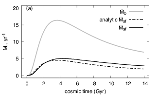
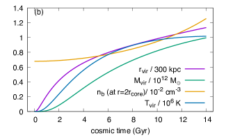
Figure 2: (a) The solid gray line is the baryon accretion rate $\dot{M}_{\rm b}(t)$. The broken black line is the analytical estimate of the star formation rate given by the equation (36) with setting $f_{\rm ms}=0.22$, $\eta_{\rm w}=6.58$, and $\dot{\Sigma}_{\rm cl}=\dot{\Sigma}_{\rm fb}=0$. (see, section 2.2 and 2.3). The black solid line shows the numerical results of the star formation rate for the fiducial model (see, section 3). (b) The purple line shows the virial radius $r_{\rm vir}(t)$, which becomes $r_{\rm vir}\simeq 342$ kpc at $t=14$ Gyr. The green line shows the virial mass of the DM halo $M_{\rm vir}$. The number density of the accreting baryon at $r=2r_{\rm core}$ is shown by the orange line as $n_{\rm b}(t,2r_{\rm core})=f_{\rm cb}\rho_{\rm dm}(t,2r_{\rm core})/m_{\rm p}$. The blue line shows the virial temperature which is given by the equation (1).

The mass density of the DM halo, $\rho_{\rm dm}(t,r)$, is assumed to be spherically symmetric with the NFW density profile (Navarro et al. (1996, 1997)). We assume the core radius to be $r_{\rm core}(t)=r_{\rm vir}(t)/20$, where $r_{\rm vir}(t)$ is the virial radius defined in the equation (1) of Rodríguez-Puebla et al. (2016). In this paper, we assume that the mass density of the accreting baryon is proportional to the DM mass density as $\rho_{\rm b}(t,r)=f_{\rm cb}\rho_{\rm dm}(t,r)$, which is shown in Figure 2b in terms of the number density $n_{\rm b}=\rho_{\rm b}/m_{\rm p}$ at the radius of $r=2r_{\rm core}$, where $m_{\rm p}$ is the proton mass. The virial temperature, defined as

$$k_{\rm B}T_{\rm vir}=\frac{2}{3}\frac{GM_{\rm vir}m_{\rm p}}{r_{\rm vir}},$$ (1)

is also shown, where $k_{\rm B}$ is the Boltzmann constant.

2.2 the galactic disk and hot gas layer

The galactic gas disk can be modeled by a viscous accretion disk. The local turbulent viscosity leads to the transport of the angular momentum (Shakura & Sunyaev (1973)). The disk wind and mass accretion are responsible for the change in total angular momentum (Suzuki & Inutsuka (2009); Suzuki et al. (2010, 2016)). We apply this disk model to the Galactic gas disk following Suzuki et al. (2016).

Under the axisymmetric approximation, the equation of the continuity and the conservation of the angular momentum can be written as (Balbus & Hawley, 1998),

$$\frac{\partial\rho}{\partial t}+\frac{1}{R}\frac{\partial}{\partial R}\left(\rho Rv_{R}\right)+\frac{\partial}{\partial z}\left(\rho v_{z}\right)=0,$$ (2)

and

$$\frac{\partial}{\partial t}\left(\rho Rv_{\phi}\right)+\frac{1}{R}\frac{\partial}{\partial R}\left[R^{2}\left(\rho v_{R}v_{\phi}-\frac{B_{R}B_{\phi}}{4\pi\rho}\right)\right]$$

$$+\frac{\partial}{\partial z}\left[\rho R\left(v_{\phi}v_{z}-\frac{B_{\phi}B_{z}}{4\pi\rho}\right)\right]=0,$$ (3)

respectively. $\rho$ is the mass density and the other symbols have their usual meaning. The azimuthal velocity is decomposed into the mean galaxy rotation velocity ${\cal V}_{\phi}$ and the turbulent perturbation $\delta v_{\phi}$ as $v_{\phi}={\cal V}_{\phi}+\delta v_{\phi}$. We assume that the rotation velocity of the gaseous matter is given by the equilibrium condition between the radial gravitational force, $g_{\rm R}=\partial\Phi/\partial R$, and centrifugal force ${\cal V}_{\phi}{}^{2}/R$, where $\Phi$ is the gravitational potential and ${\cal V}_{\phi}=\sqrt{R\big{|}g_{R}\big{|}}$. For the numerical calculation of $\Phi$, we consider the mass components of the disk gas, stars, and the DM halo. The stars and the disk gas are approximated at the midplane ($z=0$). In this case, the potential can be calculated as the sum of uniform rings of width $\Delta R$ at each discretized radius (see, Krough et al. (1982) and Lass & Blitzer (1983)), where $\Delta R$ is the interval of radial coordinates. Then, from the equation (2.2) and multiples of the equation (2) and $R{\cal V}_{\phi}$, we obtain

$$\rho Rv_{R}\times\frac{1}{R}\frac{\partial}{\partial R}\left(R{\cal V}_{\phi}\right)=-\left[\frac{1}{R}\frac{\partial}{\partial R}\left(\rho R^{2}\alpha_{R\phi}\right)+\frac{\partial}{\partial z}\left(\rho R\alpha_{\phi z}\right)\right]$$

where we approximate $\partial(\rho Rv_{\phi})/\partial t\approx R{\cal V}_{\phi}\partial\rho/\partial t$ and use the $\alpha$ prescription (Shakura & Sunyaev (1973)); $\alpha_{R\phi}\equiv v_{R}\delta v_{\phi}-B_{R}B_{\phi}/4\pi\rho$ and $\alpha_{R\phi}\equiv v_{R}\delta v_{\phi}-B_{R}B_{\phi}/4\pi\rho$. When $\partial(R{\cal V}_{\phi})/\partial R=0$ (there is no radial gradient in the specific angular momentum), we regard $\partial\rho/\partial t=0$ from the equation (2.2). For $\partial(R{\cal V}_{\phi})/\partial R\neq 0$, substituting the equation (2.2) to the equation of the continuity, we obtain

$$\frac{\partial\rho}{\partial t}-\frac{1}{R}\frac{\partial}{\partial R}\left[\frac{R}{{\cal V}_{\phi}+R{\cal V}_{\phi}{}^{\prime}}\left\{\frac{1}{R}\frac{\partial}{\partial R}\left(\rho R^{2}\alpha_{R\phi}\right)+\frac{\partial}{\partial z}\left(\rho R\alpha_{\phi z}\right)\right\}\right]$$

$$+\frac{\partial}{\partial z}\left(\rho z\right)=0,$$ (5)

where ${\cal V}_{\phi}{}^{\prime}=\partial{\cal V}_{\phi}/\partial R$. Integrating this equation along the vertical direction $z$ from the bottom surface ($z=-H/2$) to the top surface ($z=H/2$), we can derive

$$\frac{\partial\left(R\Sigma\right)}{\partial t}-\frac{1}{R}\frac{\partial}{\partial R}\left[\frac{R}{{\cal V}_{\phi}+R{\cal V}_{\phi}{}^{\prime}}\left\{\frac{1}{R}\frac{\partial}{\partial R}\left(\Sigma R^{2}C_{s}{}^{2}\bar{\alpha}_{R\phi}\right)\right.\right.$$

$$\left.\left.+\frac{\partial}{\partial z}\left(\Sigma RC_{s}{}^{2}\bar{\alpha}_{\phi z}\right)\right\}\right]=-\left[\rho Rv_{z}\right]^{H/2}_{-H/2},$$ (6)

where $\Sigma=\int\rho dz$ is the surface mass density, $\bar{\alpha}_{R\phi}\equiv\int\rho\alpha_{R\phi}dz/C_{s}{}^{2}\Sigma$, and $\bar{\alpha}_{\phi z}\equiv\rho R\alpha_{\phi z}/C_{s}{}^{2}\Sigma$. $C_{s}$ is the sound speed of the disk gas. In this paper, we approximate $\Sigma=\rho H$ and fix the disk thickness as $H=300$ pc and $C_{s}=10~{}{\rm km~{}s^{-1}}$ for simplicity. The $[\rho Rv_{z}]$ term on the right-hand side represents the effects of outflow and accretion. We denote these two effects separately as $-[\rho Rv_{z}]=-R\dot{\Sigma}_{\rm blown}+R\dot{\Sigma}_{\rm acc}$. $\dot{\Sigma}_{\rm blown}$ indicates the mass transfer rate from the disk to the hot gas layer due to the supernova explosions and $\dot{\Sigma}_{\rm acc}$ indicates the net mass accretion rate. Adding the source terms due to the star formation ($-\dot{\Sigma}_{\rm sf}$) and mass ejection by supernovae ($\dot{\Sigma_{\rm ej}}$), we finally obtain the diffusion-convection type equation as

$$\frac{\partial}{\partial t}\left(R\Sigma\right)-{\cal D}_{\Sigma}\frac{\partial^{2}}{\partial R^{2}}\left(R\Sigma\right)-{\cal V}_{\Sigma}\frac{\partial}{\partial R}\left(R\Sigma\right)-{\cal Q}_{\Sigma}\left(R\Sigma\right)$$

$$=-R\dot{\Sigma}_{\rm blown}+R\dot{\Sigma}_{\rm acc}-R\dot{\Sigma}_{\rm sf}+R\dot{\Sigma}_{\rm ej}.$$ (7)

The coefficients ${\cal V}_{\Sigma}$, ${\cal D}_{\Sigma}$, and ${\cal Q}_{\Sigma}$ can be derived by simple algebra. We assume that the $\alpha$-coefficients are constant; $\bar{\alpha}_{R\phi}=\bar{\alpha}_{\phi z}=10^{-6}$. In the realistic Galactic disk, the mass transfer speed may not exceed the typical sound velocity $C_{s}\approx 10~{}{\rm km~{}s^{-1}}$, which is a consequence of the very efficient Ly$\alpha$ cooling of the neutral hydrogen atoms. The sound crossing time of the galactic length scale is $\sim 10~{}{\rm kpc}/C_{s}\sim 1$ Gyr,i.e. the radial mass transfer dose not affect the evolution so much and the galactic radial profile depends strongly on the source terms. Therefore, we choose the small $\alpha$-coefficients to safely reproduce the realistic situation.

The mass consumption rate due to the star formation is estimated as $-\dot{\Sigma}_{\rm sf}=-\epsilon_{\rm sf}\Sigma/\tau_{\rm sf}$, where $\tau_{\rm sf}$ and $\epsilon_{\rm sf}$ are the star formation time and efficiency, respectively. From the state-of-the-art studies, the present day star formation rate is determined by the molecular cloud formation that is driven through multiple compressions of diffuse gas by supernovae (Inoue & Inutsuka (2009, 2012); Inutsuka et al. (2015); Hennebelle & Inutsuka (2019); Pineda et al. (2022)). Thus, we set the star formation time as $\tau_{\rm sf}=100~{}{\rm pc}/C_{s}\simeq 9.8~{}{\rm Myr}$, where the length scale of $100$ pc is assumed to be a typical size of local bubbles (e.g., Zucker et al. (2022) in the solar neighborhood and Watkins et al. (2023) in NGC 628). By simply adopting the Kennicutt-Schmidt law (Kennicutt & Evans (2012)), we set the star formation efficiency as

$$\epsilon_{\rm sf}=0.01\left(\frac{\Sigma}{10~{}M_{\odot}~{}{\rm pc^{-2}}}\right)^{0.4},$$ (8)

which results in $\dot{\Sigma}_{\rm sf}\propto\Sigma^{1.4}$ and the effective star formation time scale as $\tau_{\rm sf}/\epsilon_{\rm sf}\simeq 1~{}{\rm Gyr}(\Sigma/10~{}M_{\odot}~{}{\rm pc}^{-2})^{-0.4}$. For the numerical calculation, we set a threshold mass density of $R\Sigma\Delta R=10^{3}~{}M_{\odot}$ below which $\dot{\Sigma}_{\rm sf}=0$.

The surface mass density of long-lived low-mass stars and that of short-lived massive stars are calculated separately as

$$\frac{d\Sigma_{*}}{dt}=\left(1-f_{\rm ms}\right)\dot{\Sigma}_{\rm sf},$$ (9)

and

$$\frac{d\Sigma_{\rm ms}}{dt}=f_{\rm ms}\dot{\Sigma}_{\rm sf}-\dot{\Sigma}_{\rm sn},$$ (10)

where $\Sigma_{*}$ and $\Sigma_{\rm ms}$ are the surface mass densities of the low-mass stars and massive stars, respectively. We will discuss the treatments of the left-hand side terms, $d\Sigma_{*}/dt$ and $d\Sigma_{\rm ms}/dt$, later. $f_{\rm ms}$ is a mass fraction of the massive stars resulting in supernova explosions at the end of their life. $\dot{\Sigma}_{\rm sn}$ is the supernova rate in terms of the surface mass density. The massive star fraction, $f_{\rm ms}$, is estimated from the initial mass function by following the arguments of Inutsuka et al. (2015); $f_{\rm ms}=\left(8~{}M_{\odot}/m_{*,{\rm min}}\right)^{2-\beta}$, where $\beta=2.35$ corresponds to the Salpeter power-law index for a higher stellar mass part and $m_{*,{\rm min}}$ is the effective minimum stellar mass parametrizing the shape of a lower stellar mass part. In this paper, we set $m_{*,{\rm min}}=0.1~{}M_{\odot}$ and thus $f_{\rm ms}\simeq 0.22$. Note that the number fraction becomes $(8~{}M_{\odot}/m_{*,{\rm min}})^{1-\beta}\simeq 2.6\times 10^{-3}$. Then, we set $\dot{\Sigma}_{\rm sn}=\Sigma_{\rm ms}/\tau_{*,{\rm ms}}$, where $\tau_{*,{\rm ms}}$ is a typical lifetime of the massive stars. The lifetime is estimated from the mass-luminosity relation, $\tau_{*}=10~{}{\rm Gyr}(m_{*}/1~{}M_{\odot})^{-2.5}$, as

$$\tau_{*,{\rm ms}} = \left\{\int_{8M_{\odot}}^{\infty}\frac{1}{\tau_{*}}d\left(\frac{m_{*}}{1~{}M_{\odot}}\right)\right\}^{-1}$$ (11)

$$= 35\times\left(\frac{8~{}M_{\odot}}{1~{}M_{\odot}}\right)^{-3.5}{\rm Gyr}$$

$$\simeq 24.2~{}{\rm Myr}.$$

Note that the event rate of the supernova can be estimated as $\dot{\Sigma}_{\rm sn}/\bar{m}_{*,{\rm ms}}\approx f_{\rm ms}\dot{\Sigma}_{\rm sf}/\bar{m}_{*,{\rm ms}}$, where the average stellar mass of massive stars (the ratio of total mass to total number) is $\bar{m}_{*,{\rm ms}}=(\beta-1)/(\beta-2)\times 8~{}M_{\odot}\simeq 30.9~{}M_{\odot}$ and the steady-state approximation $d\Sigma_{\rm ms}/dt\approx 0$ is used. Then, the total event rate becomes $\dot{N}_{\rm sn}=f_{\rm ms}\dot{M}_{\rm sf}/\bar{m}_{*,{\rm ms}}\simeq 0.02~{}{\rm yr^{-1}}(\dot{M}_{\rm sf}/3~{}M_{\odot}~{}{\rm yr^{-1}})(m_{*,{\rm min}}/0.1~{}M_{\odot})^{\beta-2}$, where $\dot{M}_{\rm sf}=2\pi\int\dot{\Sigma}_{\rm sf}R^{2}dR$ and $\beta=2.35$ is used. This is consistent with the current state of the MW.

The supernova explosions result in the ejection of mass from $\Sigma_{\rm ms}$ to $\Sigma$, the rate of which is given by $\dot{\Sigma}_{\rm ej}$ in the equation (2.2). We suppose that each of the massive stars leaves one neutron star with a mass of $m_{*,{\rm ns}}=1.4~{}M_{\odot}$ as a result of the supernova. The net mass ejected per one supernova event is $m_{\rm ej}=\bar{m}_{*,{\rm ms}}-m_{*,{\rm ns}}$ and the mass ejection rate is $\dot{\Sigma}_{\rm ej}=(m_{\rm ej}/\bar{m}_{*,{\rm ms}})\dot{\Sigma}_{\rm sn}$. The surface mass density of the created neutron stars is given by

$$\frac{d\Sigma_{\rm ns}}{dt}=\frac{m_{*,{\rm ns}}}{\bar{m}_{*,{\rm ms}}}\dot{\Sigma}_{\rm sn}.$$ (12)

The treatment of the left-hand side term, $d\Sigma_{\rm ns}/dt$, will be discussed later.

The supernovae may also blow the gaseous matter off the disk. We suppose that some of the blown gas is responsible for the diffuse, X-ray emitting hot gas (e.g., Wada & Norman (2001); Girichidis et al. (2018)). The current Galactic disk shows such diffuse X-ray emission, called the Galactic Diffuse X-ray Emissions (GDXEs). Their origin is still under debated (e.g., Koyama (2018), for reviews). Since the estimated temperature of the GDXE ($>1$ keV) is much higher than the virial temperature of the current MW ($\sim 0.1$ keV), we expect that such X-ray emitting gas gose to the Galactic halo region. Indeed, the extended soft-X-ray emission ($\sim 0.1$ keV) is observed at much higher latitudes than the case of GDXE (e.g., Nakashima et al. (2018); Predehl et al. (2020)). Thus, we regard that the blown gas enters the hot gas layer which extends from $z=H/2$ to $z=z_{\rm hl}=2$ kpc. The outflow rate from the disk into the layer, $\dot{\Sigma}_{\rm blown}$, in the right-hand side of the equation (2.2) is estimated as

$$\dot{\Sigma}_{\rm blown} = \eta_{\rm blown}\frac{m_{\rm p}}{\bar{m}_{*,{\rm ms}}}\frac{E_{\rm sn}}{k_{\rm B}T_{\rm hl}}\dot{\Sigma}_{\rm sn}\equiv\eta_{\rm w}\dot{\Sigma}_{\rm sn},$$ (13)

where $E_{\rm sn}=10^{51}~{}{\rm erg}$, and $T_{\rm hl}=3\times 10^{6}$ K are the supernova explosion energy, and the temperature of the hot gas layer, respectively. The conversion efficiency $\eta_{\rm blown}$ is treated as a free parameter in this paper. The effective outflow efficiency driven by the supernovae, $\eta_{\rm w}$, becomes

$$\eta_{\rm w} \simeq 6.58\left(\frac{\eta_{\rm blown}}{0.1}\right)\left(\frac{E_{\rm sn}}{10^{51}~{}{\rm erg}}\right)$$ (14)

$$\times \left(\frac{T_{\rm hl}}{3\times 10^{6}~{}{\rm K}}\right)^{-1}\left(\frac{\bar{m}_{*,{\rm ms}}}{30.9~{}M_{\odot}}\right)^{-1}.$$

Then, the surface mass density of the hot gas layer, $\Sigma_{\rm hl}$, is given by

$$\frac{d\Sigma_{\rm hl}}{dt}=\frac{\dot{\Sigma}_{\rm blown}}{2}-\frac{\Sigma_{\rm hl}}{z_{\rm hl}}C_{s,{\rm hl}},$$ (15)

where $C_{s,{\rm hl}}=\sqrt{k_{\rm B}T_{\rm hl}/(0.6m_{\rm p})}\simeq 200~{}{\rm km~{}s^{-1}}(T_{\rm hl}/3\times 10^{6}~{}{\rm K})^{1/2}$. The radial mass transfer in the hot gas layer is omitted for simplicity. The factor $1/2$ of the first term on the right-hand side represents the existence of the layer on both the $+z$ and $-z$ sides. The second term represents the mass loss due to the Galactic wind (discussed later). The existence of the Galactic wind is supported by Shimoda & Inutsuka (2022) for the current condition of the MW.

We can find the importance of $\eta_{\rm w}$ from the steady-state approximation for the equation (2.2),

$$-R\dot{\Sigma}_{\rm blown}+R\dot{\Sigma}_{\rm acc}-R\dot{\Sigma}_{\rm sf}+R\dot{\Sigma}_{\rm ej}\approx 0$$

and equation (10),

$$\dot{\Sigma}_{\rm sf}f_{\rm ms}-\dot{\Sigma}_{\rm sn}\approx 0.$$

From these equations, we obtain $\dot{\Sigma}_{\rm ej}\approx(m_{\rm ej}/\bar{m}_{*,{\rm ms}})f_{\rm ms}\dot{\Sigma}_{\rm sf}$, $-\dot{\Sigma}_{\rm blown}\approx-f_{\rm ms}\eta_{\rm w}\dot{\Sigma}_{\rm sf}$, and

$$\dot{\Sigma}_{\rm sf}\approx\frac{\dot{\Sigma}_{\rm acc}}{1-f_{\rm ms}+f_{\rm ms}\eta_{\rm w}},$$ (16)

where we use $m_{\rm ej}/\bar{m}_{*,{\rm ms}}\simeq 1$. The denominator is about $2.2$ for which $f_{\rm ms}\simeq 0.22$ and $\eta_{\rm w}\simeq 6.58$ ($f_{\rm ms}\eta_{\rm w}\simeq 1.42$). Shimoda & Inutsuka (2022) showed that the mass transfer rate by the wind is comparable to the current star formation rate of several $M_{\odot}~{}{\rm yr^{-1}}$, which is consistent with the estimated $\dot{\Sigma}_{\rm blown}\simeq 1.42\dot{\Sigma}_{\rm sf}$. Thus, our choice of the conversion efficiency $\eta_{\rm blown}=0.1$ can be reasonable and the star formation rate can be about half of the net accretion rate $\dot{\Sigma}_{\rm acc}$. Note that the current cosmological accretion rate of baryons estimated from the $N$-body simulations by Rodríguez-Puebla et al. (2016) is about $7~{}M_{\odot}~{}{\rm yr^{-1}}$ (see, Figure 2a). Thus, the current star formation rate can be $\sim 3~{}M_{\odot}~{}{\rm yr^{-1}}$. Then, the total mass of the disk gas is $M\approx 3\times 10^{9}~{}M_{\odot}(\tau_{\rm sf}/10~{}{\rm Myr})(\epsilon_{\rm sf}/0.01)^{-1}$ and the mass ratio of the hot gas layer to the disk gas is $\approx\left(f_{\rm ms}\eta_{\rm w}z_{\rm hl}/C_{s,{\rm hl}}\right)\times 3~{}M_{\odot}~{}{\rm yr^{-1}}/M\approx 3\times 10^{-3}(z_{\rm hl}/2~{}{\rm kpc})$ which is consistent with a typical number density of the extended soft X-ray emission, $\sim 10^{-3}~{}{\rm cm^{-3}}$.

We also calculate the metal surface mass density, $\Sigma_{Z}$, to estimate the metal pollution of the CGM which is related to the net accretion rate $\dot{\Sigma}_{\rm acc}$ (discussed later). The differential equation of the metal surface density is assumed to be the same form as the equation (2.2), except for $\dot{\Sigma}_{\rm ej}$ and $\dot{\Sigma}_{\rm blown}$. The other differential equations of the stellar surface mass densities have the same form as those of the total surface mass densities ($\Sigma_{*}\rightarrow\Sigma_{Z,*}$, $\Sigma_{\rm ms}\rightarrow\Sigma_{Z,{\rm ms}}$, etc.). We include the newly created metal mass in the mass ejection rate as

$$\dot{\Sigma}_{Z,{\rm ej}}=\left(\frac{m_{\rm ej}}{\bar{m}_{*,{\rm ms}}}+\frac{m_{\rm co}}{\bar{m}_{*,{\rm ms}}}\right)\dot{\Sigma}_{Z,{\rm sn}},$$ (17)

where $\dot{\Sigma}_{Z,{\rm sn}}=\Sigma_{Z,{\rm ms}}/\tau_{*,{\rm ms}}$. $m_{\rm co}$ is the CO core mass in a massive star. The mass ratio of the massive star to the CO core is calculated as $\sim 1/6\mathchar 45\relax 1/4$ (e.g., Sukhbold et al. (2018); Chieffi & Limongi (2020)). In this paper, we fix $\bar{m}_{\rm co}/\bar{m}_{*,{\rm ms}}=1/6$ for simplicity. The metal outflow rate is set to $\dot{\Sigma}_{Z,{\rm blown}}=(\Sigma_{Z}/\Sigma)\dot{\Sigma}_{\rm blown}$.

Here we describe the terms $d\Sigma_{*}/dt$, $d\Sigma_{\rm ms}/dt$, and $d\Sigma_{\rm ns}/dt$. For the short-lived massive-stars, we approximate $d\Sigma_{\rm ms}/dt=\partial\Sigma_{\rm ms}/\partial t$. Since the gravitational potential evolves with time, the long-lived low-mass stars and neutron stars can move away from their birthplace (Chandrasekhar (1943)). In this paper, we omit the motion along the $z$-direction for simplicity. Then, for the numerical calculation, we introduce ”parcels” consisting of the formed stars at each time step and each radial position $(t^{n},R_{i})$ and solve for their motion;

$$\frac{d^{2}R_{*,j}}{dt^{2}}=-g_{R}(t,R_{*,j})+\frac{v_{*,\phi,j}{}^{2}}{R_{*,j}},$$ (18)

where $R_{*,j}$ and $v_{*,\phi,j}$ are the position and rotation velocity of the parcel denoted by the subscript $j$, respectively. Note that $R_{*,j}v_{*,\phi,j}$ is constant. The net surface density of the mass is calculated as

$$R\Sigma_{*}(t,R)=\sum_{j}\delta m_{*,j}\exp\left[-\frac{(R-R_{*,j})^{2}}{2H^{2}}\right],$$ (19)

where $\delta m_{*,j}$ is the line mass of parcel $j$. Let $t_{{\rm birth},j}$ be the birthtime of the stellar objects in the parcel $j$ at $(t^{n},R_{i})$. Then, the birthplace is written as $R_{{\rm birth},j}=R_{*,j}(t_{{\rm birth},j})=R_{i}$. We assume the initial radial velocity as $v_{*,R,j}(t_{{\rm birth},j})=dR_{*,j}/dt=0$ and the initial rotation velocity as $v_{*,\phi,j}(t_{\rm birth})={\cal V}_{\phi}(t_{\rm birth},R_{\rm birth})$. The mass of parcel $j$ is given by $\delta m_{*,j}=R_{\rm birth}\dot{\Sigma}_{\rm sf}(t_{\rm birth},R_{\rm birth})\Delta t$ for the low-mass stars and $\delta m_{*,j}=R_{\rm birth}\dot{\Sigma}_{\rm ns}(t_{\rm birth},R_{\rm birth})\Delta t$ for the neutron stars, respectively, where $\Delta t$ is the time interval of the numerical calculation. To save the computation costs, we implement that parcels $j$ and $k$ are unified under the conditions of $|R_{*,j}-R_{*,k}|<10^{-2}$, $|v_{*,\phi,j}-v_{*,\phi,k}|<10^{-2}$, $|v_{*,R,j}-v_{*,R,k}|<10^{-2}$, and $v_{*,R,j}v_{*,R,k}>0$ to have a mass of $\delta m_{*,j}+\delta m_{*,k}$. The information of the birthtime and place are evaluated as $(\delta m_{*,j}t_{{\rm birth},j}+\delta m_{*,k}t_{{\rm birth},k})/(\delta m_{*,j}+\delta m_{*,k})$ and $(\delta m_{*,j}R_{{\rm birth},j}+\delta m_{*,k}R_{{\rm birth},k})/(\delta m_{*,j}+\delta m_{*,k})$, respectively. We set the inner and outer boundary conditions. For $R_{*,j}<\Delta R$, we regard the parcel to drop the galactic center $R=0$ and its motion is no longer calculated. For $R_{*,j}>3R_{\rm B}$, where $R_{\rm B}=30$ kpc is the outer boundary of the gas disk calculation, we regard the parcel to escape from the system.

We summarize the disk model;

$$\frac{\partial}{\partial t}\left(R\Sigma\right)-{\cal D}_{\Sigma}\frac{\partial^{2}}{\partial R^{2}}\left(R\Sigma\right)-{\cal V}_{\Sigma}\frac{\partial}{\partial R}\left(R\Sigma\right)$$ (20)

$$=-R\dot{\Sigma}_{\rm blown}+R\dot{\Sigma}_{\rm acc}-R\dot{\Sigma}_{\rm sf}+R\dot{\Sigma}_{\rm ej},$$

$$\frac{d\Sigma_{*}}{dt}=\left(1-f_{\rm ms}\right)\dot{\Sigma}_{\rm sf},$$

$$\frac{d\Sigma_{\rm ms}}{dt}=f_{\rm ms}\dot{\Sigma}_{\rm sf}-\dot{\Sigma}_{\rm sn},$$

$$\frac{d\Sigma_{\rm ns}}{dt}=\frac{m_{*,{\rm ns}}}{\bar{m}_{*,{\rm ms}}}\dot{\Sigma}_{\rm sn},$$

$$\frac{d\Sigma_{\rm hl}}{dt}=\frac{\dot{\Sigma}_{\rm blown}}{2}-\frac{\Sigma_{\rm hl}}{z_{\rm hl}}C_{s,{\rm hl}},$$

$$\dot{\Sigma}_{\rm sf}=\frac{\epsilon_{\rm sf}}{\tau_{\rm sf}}\Sigma,$$

$$\dot{\Sigma}_{\rm ej}=\frac{m_{\rm ej}}{m_{*,{\rm ms}}}\dot{\Sigma}_{\rm sn}~{}~{}~{}\left[\dot{\Sigma}_{Z,{\rm ej}}=\left(\frac{m_{\rm ej}}{\bar{m}_{*,{\rm ms}}}+\frac{m_{\rm co}}{\bar{m}_{*,{\rm ms}}}\right)\dot{\Sigma}_{Z,{\rm sn}}~{}({\rm for~{}metals})\right],$$

$$\dot{\Sigma}_{\rm sn}=\frac{\Sigma_{\rm ms}}{\tau_{*,{\rm ms}}},$$

$$\dot{\Sigma}_{\rm blown}=\eta_{\rm w}\dot{\Sigma}_{\rm sn}~{}~{}~{}\left[\dot{\Sigma}_{Z,{\rm blown}}=\frac{\Sigma_{Z}}{\Sigma}\dot{\Sigma}_{\rm blown}~{}({\rm for~{}metals})\right].$$

The metal surface mass densities are denoted by replacing the symbols as $\Sigma\rightarrow\Sigma_{Z}$, $\Sigma_{*}\rightarrow\Sigma_{Z,*}$, $\dot{\Sigma}_{\rm sf}\rightarrow\dot{\Sigma}_{Z,{\rm sf}}=(\epsilon_{\rm sf}/\tau_{\rm sf})\Sigma_{Z}$ and so on, except for $\dot{\Sigma}_{Z,{\rm ej}}$ and $\dot{\Sigma}_{Z,{\rm blown}}$. We find that $\Sigma$ is conserved (take $\dot{\Sigma}_{\rm blown}=\dot{\Sigma}_{\rm scc}=0$ and $\Sigma_{\rm hl}=0$), while $\Sigma_{Z}$ increases at a rate of $(m_{\rm co}/\bar{m}_{*,{\rm ms}})\dot{\Sigma}_{\rm sn}$.

The estimation of the total mass of metal ejected by the supernovae clarifies the importance of the galactic wind (i.e. the role of the CRs). When the star formation continues with a constant rate of $\sim 3~{}M_{\odot}~{}{\rm yr}^{-1}$ throughout the cosmic age, the total metal mass ejected by supernovae becomes $\sim(m_{\rm co}/\bar{m}_{*,{\rm ms}})f_{\rm ms}\times 3~{}M_{\odot}~{}{\rm yr}^{-1}\times 14~{}{\rm Gyr}\sim 1.54\times 10^{9}~{}M_{\odot}$, where $\dot{\Sigma}_{\rm sn}\approx f_{\rm ms}\dot{\Sigma}_{\rm sf}$ is used. The total mass of the disk gas, $\sim 3\times 10^{9}~{}M_{\odot}$, which is comparable to the estimated metal mass, implies the existence of the wind; the almost all metals should be expelled from the disk to simultaneously explain the total mass of the disk gas and the metallicity of $Z_{\odot}\sim 0.01$ in the current Galactic disk. If the metal polluted gas is well mixed with the primordial gas with a mass of $f_{\rm cb}M_{\rm vir,0}\sim 10^{11}~{}M_{\odot}$, the mean metallicity becomes $\sim 10^{9}~{}M_{\odot}/10^{11}_{\odot}\sim 0.01$, which is consistent with the solar metallicity. Thus, the CRs also play a key role in controling an amount of the metals in the Galactic disk by driving the wind.

2.3 the galactic halo region; wind, CGM, and IGM

We suppose that the galactic wind is driven by CRs from the upper boundary of the hot gas layer, $z=z_{\rm hl}=2$ kpc, with a rate of $(\Sigma_{\rm hl}/z_{\rm hl})C_{s,{\rm hl}}$ following Shimoda & Inutsuka (2022). The CRs are assumed to be accelerated by supernova remnant shocks. In the following, we discuss the CR energy density and describe the numerical modeling of the galactic halo gas. In our model, the disk accretion rate, $R\dot{\Sigma}_{\rm acc}$, is decomposed into three components as

$$R\dot{\Sigma}_{\rm acc}=R\dot{\Sigma}_{\rm b,disk}+R\dot{\Sigma}_{\rm fb}+R\dot{\Sigma}_{\rm cl},$$ (21)

where the $\dot{\Sigma}_{\rm b,disk}$ is the cosmological baryon accretion rate on the disk, $\dot{\Sigma}_{\rm fb}$ is the mass coming from the wind region, and $\dot{\Sigma}_{\rm cl}$ is the mass accretion rate from the metal-polluted CGM, respectively. Note that our model calculation of the disk is done by the line mass of $R\Sigma$ as shown in the equation (20).

Shimoda et al. (2022) recently suggested that the energy injection rate of CRs at the shocks can be about 10 % of the supernova explosion energy by modeling the ion heating process at the shock transition. We follow their results and set the CR energy injection rate (${\rm erg~{}s^{-1}~{}cm^{-3}}$) as

$$\dot{q}_{\rm cr}=\frac{\eta_{\rm cr}E_{\rm sn}}{H\bar{m}_{*,{\rm ms}}}\dot{\Sigma}_{\rm sn},$$ (22)

where $\eta_{\rm cr}\sim 0.1$ is the injection efficiency. The energy loss rate of the CRs via the hadronic interactions (${\rm erg~{}s^{-1}~{}cm^{-3}}$) can be approximated by

$$-{\cal L}_{\rm cr}=-\Lambda_{\rm h}\frac{\Sigma}{m_{\rm p}H}e_{\rm cr},$$ (23)

where $\Lambda_{\rm h}=7.44\times 10^{-16}~{}{\rm s^{-1}~{}cm^{3}}$ is the collision rate per particle (see, Pfrommer et al. (2017) for details), and $e_{\rm cr}~{}({\rm erg~{}cm^{-3}})$ is the energy density of the CRs. We presume that the acceleration time of CRs at each supernova remnant shock is quite short, at most $\sim 10^{4}$ yr, which is a typical radiative cooling time of the shock-heated plasma for an ambient density of $\sim 1~{}{\rm cm^{-3}}$ (e.g., Vink et al. (2006)). Thus, we approximate the energy density of the CRs around their source as $\dot{q}_{\rm cr}-{\cal L}_{\rm cr}\approx 0$, i.e.,

$$e_{\rm cr,source}=\frac{\eta_{\rm cr}E_{\rm sn}}{\Lambda_{\rm h}}\frac{m_{\rm p}}{\bar{m}_{*,{\rm ms}}}\frac{\dot{\Sigma}_{\rm sn}}{\Sigma}.$$ (24)

Note that $e_{\rm cr,source}$ is assumed to be uniform along the vertical direction $z$ in the disk. The injected CRs will escape from the galaxy. In this paper, the escape flux is assumed to be dominated by the diffusion effect (the convection effect is omitted for simplicity). Then, we approximate the CR energy density released around the sources as

$${\cal D}_{\rm cr}{\bm{\nabla}}^{2}e_{\rm cr}=\frac{e_{\rm cr,source}}{\tau_{\rm cr,esc}},$$ (25)

where $\cal{D}_{\rm cr}$ and $\tau_{\rm cr,esc}$ are the CR diffusion coefficient and the CR escape time from the galaxy, respectively. The escape time is estimated by the abundance of CR nuclei (e.g., the Boron-to-Carbon ratio) as $\sim 10$ Myr. The diffusion coefficient is estimated from the abundance ratio with the assumption that the CR scale height of $\sim$ kpc; ${\cal D}_{\rm cr}=3\times 10^{28}~{}{\rm cm^{2}~{}s^{-1}}$ is frequently used (e.g., Gabici et al. (2019)). In this paper, we parametrize the CR scale height, $H_{\rm cr}=\sqrt{{\cal D}_{\rm cr}\tau_{\rm cr,esc}}$. Then, the CR energy densities are estimated by using the steady-state approximation of $\dot{\Sigma}_{\rm sn}\approx f_{\rm ms}\dot{\Sigma}_{\rm sf}$ and $\Sigma\approx(\tau_{\rm sf}/\epsilon_{\rm sf})\dot{\Sigma}_{\rm sf}$ as

$$e_{\rm cr,source} \approx \frac{\eta_{\rm cr}E_{\rm sn}}{\tau_{\rm sf}\Lambda_{\rm h}}\frac{m_{\rm p}}{\bar{m}_{*,{\rm ms}}}f_{\rm ms}\epsilon_{\rm sf}$$ (26)

$$\approx 16~{}{\rm eV~{}cm^{-3}}\left(\frac{\eta_{\rm cr}}{0.1}\right)\left(\frac{f_{\rm ms}}{0.22}\right)$$

$$\times \left(\frac{\tau_{\rm sf}/\epsilon_{\rm sf}}{1~{}{\rm Gyr}}\right)^{-1}\left(\frac{\bar{m}_{*,{\rm ms}}}{30.9~{}M_{\odot}}\right)^{-1},$$

and by using $\bm{\nabla}^{2}e_{\rm cr}\approx e_{\rm cr}/({\rm kpc})^{2}$ as,

$$e_{\rm cr}\approx 1.8~{}{\rm eV~{}cm^{-3}}\left(\frac{e_{\rm cr,source}}{16~{}{\rm eV~{}cm^{-3}}}\right)\left(\frac{H_{\rm cr}}{3~{}{\rm kpc}}\right)^{-2}.$$ (27)

Thus, we can find that the CR energy density in the interstellar medium (ISM), which is expected to be a few ${\rm eV~{}cm^{-3}}$, is given by $\eta_{\rm cr}/{\cal D}_{\rm cr}\tau_{\rm esc}=\eta_{\rm cr}/H_{\rm cr}{}^{2}$. We treat the CR scale height $H_{\rm cr}$ as a free parameter to study the effects of CR and fix the injection efficiency as $\eta_{\rm cr}=0.1$. In the CR injection scenario proposed by Shimoda et al. (2022), the injection efficiency depends on the sonic Mach number of the collisionless shocks. Therefore, we regard that the efficiency $\eta_{\rm cr}$ is universally determined by the local physics. On the other hand, the diffusion coefficient may depend on the local magnetic field strength whose evolution over cosmic time may still be uncertain. Moreover, there is no consensus on the general expression of the CR diffusion coefficient. Note that the energy densities depend on the star formation rate via $(\tau_{\rm sf}/\epsilon_{\rm sf})^{-1}\propto\Sigma^{0.4}$; a larger $\Sigma$ results in a larger star formation rate and a larger CR energy density. To estimate the CR energy density, we omit non-trivial numerical factors, so for simplicity we chose $H_{\rm cr}=3$ kpc. From the numerical results discussed later, we find that $(\eta_{\rm cr},H_{\rm cr})=(0.1,10~{}{\rm kpc})$ produces a reasonable result. The height of $H_{\rm cr}=10$ kpc is consistent with recent theoretical model of CR transport (Evoli et al. (2020)).

The galactic wind is driven by the CR pressure, $P_{\rm cr}=(\gamma_{c}-1)e_{\rm cr}$, where $\gamma_{c}=4/3$, from the hot gas layer. Shimoda & Inutsuka (2022) showed that for the current conditions of the MW, the wind density and temperature can be nearly constant at $z\lesssim 10$ kpc due to the balance between the radiative cooling and effects of CR heating. The thermal gas pressure and the CR pressure are comparable to each other. From these results, we simplify the wind dynamics as

$$\frac{d\bm{v}_{\rm w}}{dt}=-\frac{\bm{\nabla}P_{\rm cr}}{\rho_{\rm w}}-\bm{g},$$ (28)

where we approximate the total pressure as $P\approx P_{\rm cr}$. $\rho_{\rm w}$ and $\bm{v}_{\rm w}$ are the mass density and velocity of the wind, respectively. $\bm{g}$ is the gravitational acceleration calculated from the Poisson equation with the DM component and the disk mass components ($\Sigma$, $\Sigma_{*}$, $\Sigma_{\rm ms}$, and $\Sigma_{\rm ns}$). For numerical calculations of the wind, we treat the fluid parcel as a test particle denoted by the subscript $k$ and adopt the equation (28) as its equation of motion under the axisymmetric approximation. The density $\rho_{{\rm w},k}$ is assumed to be constant. For each time step, new particles are newly introduced at each point of $(R_{i},z_{\rm hl})$. The initial conditions of the particles are assumed to be $\rho_{{\rm w},k}=\Sigma_{\rm hl}(t,R)/z_{\rm hl}$, $v_{{\rm w},R,k}=0$, $v_{{\rm w},\phi,k}=\sqrt{Rg_{R}(t,R,z_{\rm hl})}$, and $v_{{\rm w},z,k}=C_{\rm s,hl}$, where $g_{R}$ is the radial component of $\bm{g}$ and the centrifugal force equilibrium is assumed, $v_{{\rm w},\phi}{}^{2}/R=g_{R}$. The mass of each particle is assumed to be $dm_{{\rm w},k}=\rho_{{\rm w},k}C_{s,{\rm hl}}R\Delta R\Delta td\phi=$constant. The infinitesimal azimuthal element vanishes by the axisymmetric integration. Using the particles located at $|z|<H/2$ and $R<R_{\rm B}$ with a density of $\rho_{{\rm w},k}\leq\Sigma(t,R_{k})/H$, where $R_{\rm B}=30$ kpc is the outer boundary of the disk region, we calculate the accretion rate component, $R\dot{\Sigma}_{\rm fb}$, as

$$R\dot{\Sigma}_{\rm fb}(t,R)=2\int_{0}^{2\pi}\sum_{k}\frac{dm_{{\rm w},k}}{d\phi}\frac{N_{k}}{\Delta t}\exp\left[-\frac{(R-R_{k})^{2}}{2H^{2}}\right]d\phi,$$

where $N_{k}=(\int_{0}^{R_{\rm B}}e^{-(R-R_{k})^{2}/2H^{2}}dR)^{-1}$ is the normalization factor. Note that the metal mass is calculated by the same manner as the total mass.

We regard that the particles located at $r_{k}>r_{\rm cgm}$ enter the CGM region, where $r_{k}=\sqrt{R_{k}{}^{2}+z_{k}{}^{2}}$ and $r_{\rm cgm}=2~{}r_{\rm core}(t)$ is the boundary galactocentric radius between the wind region and CGM region. The total CGM mass, $M_{\rm cgm}(t)$, is calculated as

$$\frac{dM_{\rm cgm}}{dt}=\dot{M}_{\rm w}+\dot{M}_{\rm ex}-\dot{M}_{\rm cl},$$ (30)

where

$$\dot{M}_{\rm w}=2\int_{0}^{2\pi}\sum_{k}\frac{dm_{{\rm w},k}}{d\phi}d\phi,$$ (31)

and $\dot{M}_{\rm ex}$ represents the mass supply due to the interaction between the wind and the baryon accretion flow. Some of the accreting baryons from the IGM may be expelled by the wind entering the CGM region. For simplicity, we assume that $\dot{M}_{\rm ex}=\dot{M}_{\rm w}$. $\dot{M}_{\rm cl}$ is the mass loss of the CGM due to the metal pollution which results in a large radiative cooling rate. For the CGM of externalgalaxies, absorption lines of lower ionized species such as HI, CII, and MgII are observed (Tumlinson et al. (2017), and references therein). The existence of such lower ionized species implies the existence of condensation phenomena that shield the cool gas from ionizing photons (e.g., the metagalactic radiation field, see Gnat (2017)). We assume that such cool, condensed gas leaves from the CGM by losing its angular momentum at a rate of

$$-\dot{M}_{\rm cl}=-\frac{\epsilon_{\rm cgm}}{\tau_{\rm cool}}M_{\rm cgm}=-\frac{\epsilon_{\rm cgm}kT_{\rm cgm}}{n_{\rm cgm}\Lambda_{{\rm rad},\odot}}\frac{Z_{\rm cgm}}{Z_{\odot}}M_{\rm cgm},$$ (32)

where $n_{\rm cgm}$ is the mean number density estimated as

$$n_{\rm cgm}=\frac{3}{4\pi r_{\rm vir}{}^{3}}\frac{M_{\rm cgm}}{m_{\rm p}},$$ (33)

and the radiative cooling time is estimated as

$$\tau_{\rm cool}=\frac{n_{\rm cgm}\Lambda_{{\rm rad},\odot}}{kT_{\rm cgm}}\frac{Z_{\odot}}{Z_{\rm cgm}}.$$ (34)

The mean temperature of the CGM, $T_{\rm cgm}$, is assumed to be equal to the virial temperature, $T_{\rm vir}(t)$, which is given by the equation (1). $\Lambda_{{\rm rad},\odot}(T_{\rm cgm})$ is the radiative cooling rate for the solar abundance given by Shimoda & Inutsuka (2022). $Z_{\rm cgm}$ is the metallicity of the CGM estimated as $Z_{\rm cgm}=M_{Z,{\rm cgm}}/M_{\rm cgm}$ and $Z_{\odot}=0.0134$ is the solar metallicity (Asplund et al. (2009)). $\epsilon_{\rm cgm}$ represents the efficiency of the angular momentum loss which is required for both condensation and accretion phenomena. We fix the efficiency $\epsilon_{\rm cgm}=0.01$ by analogy with $\epsilon_{\rm sf}$. The factor $Z_{\rm cgm}/Z_{\odot}$ approximately reflects the metallicity dependence of $\Lambda_{\rm rad}$.

The net baryon accretion rate onto the disk is given by $\dot{M}_{\rm b}-\dot{M}_{\rm ex}+\dot{M}_{\rm cl}$. The local accretion rate at $R$ is assumed to be

$$R\dot{\Sigma}_{\rm b,disk}(t,R) = \frac{\dot{M}_{\rm b}-\dot{M}_{\rm ex}+\dot{M}_{\rm cl}}{4\pi}$$ (35)

$$\times N_{\rm b,disk}\exp\left[-\frac{(R-r_{\rm core})^{2}}{2r_{\rm core}{}^{2}}\right],$$

where $N_{\rm b,disk}=(\int_{0}^{R_{\rm B}}e^{-(R-r_{\rm core})^{2}/2r_{\rm core}{}^{2}}dR)^{-1}$ is the normalization factor. Here, the core radius $r_{\rm core}$ is assumed to reflect a small angular momentum of the accreting gas from the IGM so that the galactic disk is formed. The radial profile of the galactic disk depends strongly on the source terms as we discussed in the equation (2.2). Since the galactic wind acts after the mass supply at a local point, the radial profile is almost given by this assumed $R\dot{\Sigma}_{\rm b.disk}$.

The estimate of the star formation rate under the steady-state approximation discussed in the equation (16) is rewritten as

$$\dot{\Sigma}_{\rm sf}\approx\frac{\dot{\Sigma}_{\rm b}+\dot{\Sigma}_{\rm fb}+\dot{\Sigma}_{\rm cl}}{1-f_{\rm ms}+2f_{\rm ms}\eta_{\rm w}},$$ (36)

where we use the total disk mass accretion rate $\dot{\Sigma}_{\rm acc}=\dot{\Sigma}_{\rm b}-\dot{\Sigma}_{\rm w}+\dot{\Sigma}_{\rm cl}+\dot{\Sigma}_{\rm fb}$ and approximate that $\dot{\Sigma}_{\rm w}\approx\dot{\Sigma}_{\rm blown}$. The dashed line in Figure 2a shows the estimated total star formation rate with $f_{\rm ms}=0.22$, $\eta_{\rm w}=6.58$, and $\dot{\Sigma}_{\rm cl}=\dot{\Sigma}_{\rm fb}=0$. Since the total mass of stars at the current MW is $\sim(4\mathchar 45\relax 6)\times 10^{10}~{}M_{\odot}$ (Bland-Hawthorn & Gerhard, 2016), and since the expected total baryon mass is $M_{\rm b}\sim f_{\rm cb}M_{\rm vir,0}\sim 10^{11}~{}M_{\odot}$, a significant fraction of gaseous matter should be deposited in the galactic halo region (Tumlinson et al., 2017). The small $\dot{\Sigma}_{\rm fb}$ and $\dot{\Sigma}_{\rm cl}$ are preferred to realize such a situation under the assumed $\dot{\Sigma}_{\rm b,disk}$ given by the equation (35).

In this paper we focus on studying the effects of $\eta_{\rm blown}$ and $H_{\rm cr}$. The conversion efficiency $\eta_{\rm blown}$ determines the relation between the star formation rate, $\dot{\Sigma}_{\rm sf}$, and the disk mass accretion rate, $\dot{\Sigma}_{\rm acc}$. The CR scale height $H_{\rm cr}$ determines the CR energy density, $e_{\rm cr}$. If the energy density is small, the galactic wind is unable to reach the CGM region; the wind gas falls back to the disk and the net mass accretion rate increases by the term of $\dot{\Sigma}_{\rm fb}$. Note that the CGM metal pollution by the galactic wind is required to explain the galactic halo observations and the typical metallicity of the current Galactic disk of $Z\sim Z_{\odot}$. $\eta_{\rm blown}$ also determines the mass transfer rate from the disk to the hot gas layer and $H_{\rm cr}$ determines that from the hot gas layer to the CGM region. The efficient metal pollution of the CGM can result in a large additional mass accretion rate $\dot{\Sigma}_{\rm cl}$. Thus, these two parameters $\eta_{\rm blown}$ and $H_{\rm cr}$ are important for the gas mass distribution and consequently for the star formation. We regard the case of $\eta_{\rm blown}=0.1$ and $H_{\rm cr}=10$ kpc as the fiducial model and summarize the other case in Table 2.3. Note that the values of $H_{\rm cr}$ are chosen to be $(10/7.07)^{2}\simeq 2$ and $(10/14.14)^{2}\simeq 0.5$.

Model parameters. Model $\eta_{\rm blown}$ $H_{\rm cr}$ category 0 $0.1$ $10$ kpc fiducial model 1 $0.2$ $10$ kpc massive wind 2 $0.05$ $10$ kpc weak wind 3 $0.1$ $7.07$ kpc large $e_{\rm cr}$ 4 $0.1$ $14.14$ kpc small $e_{\rm cr}$

For the numerical calculations, we set the time interval as $\Delta t=0.85$ Myr. Such small $\Delta t$ is required to resolve the lifetime of massive stars, $\tau_{*,{\rm ms}}\simeq 24.2$ Myr. The interval of the radial coordinate for the disk region is set to be $\Delta R=R_{\rm B}/128$. The initial time is set to $t_{0}=0.1$ Gyr, and the total baryon mass is given by the $N$-body simulation results. Then, we set $\Sigma(t_{0},R)=$constant with a total mass of $f_{\rm cb}M_{\rm vir}(t_{0})\times 10^{-2}\simeq 7.8\times M_{\odot}$. The initial mass of the CGM is $M_{\rm cgm}(t_{0})=0.99f_{\rm cb}M_{\rm vir}(t_{0})$. The stellar objects and metal masses are initially zero. Note that the results are not affected by these assumed initial conditions.

3 Results

We display the numerical results of our model for parameter the sets summarized by Table 2.3. First, we present the fiducial model, Model 0. We then discuss the difference between Model 0 and the others.

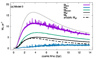
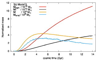
Figure 3: The numerical results of Model 0. (a) The baryon accretion rate $\dot{M}_{\rm b}$ (solid grey line), the estimated star formation rate given by the equation (36) with $\dot{\Sigma}_{\rm cl}=\dot{\Sigma}_{\rm fb}=0$ (broken black line), and the calculated star formation rate $\dot{M}_{\rm sf}$ (solid black line) are also shown in Figure 2a. The solid purple line shows the net accretion rate $\dot{M}_{\rm acc}$. The solid green line is the outflow rate of the disk $\dot{M}_{\rm blown}$. (b) The results of total mass of the CGM (red), the stellar mass (black), the gaseous matter at the disk (orange), and the wind (light blue).

Figure 3a shows the results for the total star formation rate, $\dot{M}_{\rm sf}$ (solid black line), the mass transfer rate given by the falling-back wind particles, $\dot{M}_{\rm fb}$ (purple), and the disk outflow rate, $\dot{M}_{\rm blown}$ (green). $\dot{M}_{\rm sf}$ is in good agreement with the estimated star formation rate for which $\dot{\Sigma}_{\rm cl}=\dot{\Sigma}_{\rm fb}=0$ given by the equation (36). $\dot{M}_{\rm fb}$ is small, although its contribution becomes large from $t>8$ Gyr due to a combination of disk mass growth and CR pressure decrease. Figure 3b shows the time evolution of the total mass of the CGM, $M_{\rm cgm}$, the total mass of low-mass stars, $M_{*}$, the total mass of the disk gas, $M$, and the total mass of the wind, $M_{\rm wind}$. $M_{*}\simeq 4\times 10^{10}~{}M_{\odot}$ at $t=14$ Gyr is consistent with the current condition of our galaxy (Bland-Hawthorn & Gerhard, 2016). The time evolution of $M$ is almost the same as $\dot{M}_{\rm sf}$ because of the assumed $\dot{\Sigma}_{\rm sf}=(\epsilon_{\rm sf}/\tau_{\rm sf})\Sigma$. The wind mass $M_{\rm wind}$ is flattened from $t\simeq 4$ Gyr on, when the growth of virial radius $r_{\rm vir}(t)$ almost finishes (see, Figure 2b). Since we regard the region within $r<2r_{\rm core}(t)=r_{\rm vir}(t)/10$ as the ‘wind’ region, this feature may have no useful physical meaning. The mass of the CGM increases monotonically, reflecting the cosmological accretion rate $\dot{M}_{\rm b}$ and the small mass loss rate of the CGM, $\dot{M}_{\rm cl}$.

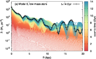
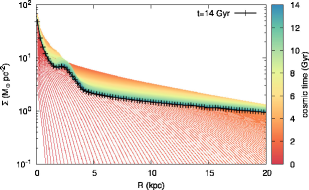
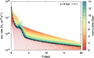
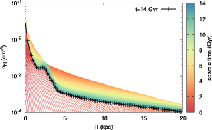
Figure 4: The radial profile of the disk and hot gas layer at each time for Model 0. (a) The surface mass density of the low-mass stars $\Sigma_{*}$. (b) The surface mass density of the gas $\Sigma$. (c) The net accretion rate $\dot{\Sigma}_{\rm acc}$. (d) The number density of the hot gas layer $n_{\rm hl}\equiv\Sigma_{\rm hl}/(z_{\rm hl}m_{\rm p})$.

Figures 4a, 4b, and 4c show the radial profiles of the surface mass densities of the low-mass stars, $\Sigma_{*}(t,R)$, that of the gas, $\Sigma(t,R)$, and the net accretion rate $\dot{\Sigma}_{\rm acc}(t,R)$ for each time, respectively. The radial profiles of $\Sigma_{*}$ and $\Sigma$ are nearly converged at $t\sim 8$ Gyr, although $\Sigma_{*}$ is perturbed by the stellar dynamics. The accretion rate, $\dot{\Sigma}_{\rm acc}$, shows drastic variations at $R\lesssim 5~{}{\rm kpc}$ from $t\sim 8$ Gyr due to the falling-back of the wind, $\dot{\Sigma}_{\rm fb}$. Although our treatment of the wind dynamics is still not sufficient (the disk is axisymmetric and the vertical motion is omitted), this result implies that the inner region of the disk is more affected by the gas accretion from the galactic halo than the outer region. The variations of $\dot{\Sigma}_{\rm acc}$ correspond to the perturbations of $\Sigma$ which in reality may have a three-dimensional, compact structure in reality (such as giant molecular clouds). If the case, the local perturbations of the gravitational potential would lead to the stellar migration phenomena (e.g., Fujimoto et al. (2023)). It would be an interesting subject to investigate the birthplace of the solar system, the morphology of galaxies especially for the formation and evolution of the Galactic bulge region, and so on. Figure 4d shows the number density profiles of the hot gas layer, $n_{\rm hl}\equiv\Sigma_{\rm hl}/(z_{\rm hl}m_{\rm p})$, which can be responsible for the extended soft X-ray emission as we discussed in section 2.2 and the steady-state solutions of the galactic wind derived by Shimoda & Inutsuka (2022).

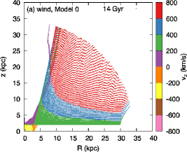
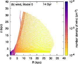
Figure 5: The numerical results of the galactic halo region for Model 0. (a) The wind profile of the vertical velocity component, $v_{{\rm w},z}$, at $t=14$ Gyr. (b) The wind profile of the number density, $n_{\rm w}\equiv\rho_{\rm w}/m_{\rm p}$, at $t=14$ Gyr.

Figures 5a and 5b are the snapshots at $t=14$ Gyr showing the vertical velocity component of the wind, $v_{{\rm w},z}$, and the number density of the wind, $n_{\rm w}\equiv\rho_{\rm w}/m_{\rm p}$, respectively. The wind morphology becomes to the so-called X-shape wind due to the centrifugal force. Such a morphology is reported in the externalgalaxy of NGC 3079 by Hodges-Kluck et al. (2020), for example. As shown in Figure 3a, most of the wind mass is transferred to the CGM region ($\dot{M}_{\rm blown}>\dot{M}_{\rm fb}$). The wind particle that leaves the radius of $R\lesssim 5$ kpc eventually falls back to the disk. This results in the metal pollution of the inner disk region. The metallicity history of the disk will be discussed later.

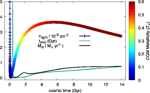
Figure 6: The numerical results of the galactic halo region for Model 0. The time evolution of the CGM number density, $n_{\rm cgm}$, radiative cooling time, $\tau_{\rm cool}$ (green line), and the mass depletion rate of the CGM, $\dot{M}_{\rm cl}$ (black line). The color bar indicates the metallicity of the CGM, $M_{Z,{\rm cgm}/M_{\rm cgm}}$.

Figure 6 shows the time evolution of the CGM number density, $n_{\rm cgm}$ (the equation 33), the radiative cooling time, $\tau_{\rm cool}$ (the equation 34), the mass depletion rate, $\dot{M}_{\rm cl}$ (the equation 32), and the metallicity, $M_{Z,{\rm cgm}}/M_{\rm cgm}$. At the very early stage $t<1$ Gyr, the very small virial radius, $r_{\rm vir}(t)$, results in the large $n_{\rm cgm}$. The large $\tau_{\rm cool}$ is due to the small metallicity of the CGM. At $t>1$ Gyr, $r_{\rm vir}$ becomes $\sim 30$ kpc (see, Figure 2b), and then the magnitudes of $n_{\rm cgm}$ and $\tau_{\rm cool}$ converge. The mass growth of the CGM due to the mass transfer by the wind is balanced with the growth of $\sim r_{\rm vir}(t)^{3}$ as a result, leading to the almost constant $n_{\rm cgm}(t)\sim 10^{-5}~{}{\rm cm}^{-3}$. The cooling time becomes $\sim 1$ Gyr, which is consistent with the steady-state solutions of the galactic wind studied by Shimoda & Inutsuka (2022). The small mass depletion rate of CGM, $\dot{M}_{\rm cl}\sim 0.5~{}{\rm M_{\odot}~{}yr^{-1}}$, is determined by the assumed efficiency of $\epsilon_{\rm cgm}=0.01$. The CGM metallicity may be sufficient to reproduce the observed metal absorption lines (see, Tumlinson et al. (2017) for a review).

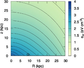
Figure 7: The numerical results of the galactic halo region for Model 0. The profile of the CR energy density, $e_{\rm cr}$, at $t=14$ Gyr. The black contours show the density increasing by $0.2~{}{\rm eV~{}cm^{-3}}$ from $1~{}{\rm eV~{}cm^{-3}}$ to $3.6~{}{\rm eV~{}cm^{-3}}$. The star symbol indicates $R=8.5$ kpc.

The CR energy density, $e_{\rm cr}$, at $t=14$ Gyr shown in Figure 7 is $2\mathchar 45\relax 4~{}{\rm eV~{}cm^{-3}}$. The radial dependence of $e_{\rm cr}$ reflects the star formation rate $\dot{\Sigma}_{\rm sf}(R)$ (see, the equation 26). Although $e_{\rm cr}$ is measured to be $\simeq 1~{}{\rm eV~{}cm^{-3}}$ around the Earth, the actual $e_{\rm cr}$ in the local ISM is still uncertain. To explain the CR ionization rates measured in the local molecular clouds, the higher energy density of $2\mathchar 45\relax 4~{}{\rm eV~{}cm^{-3}}$ may be preferred (e.g., Cummings et al. (2016)). Note that our model is based on the long-term averaged argument of the star formation with a time scale of $\sim 1$ Gyr. The CR energy density measured around the Earth reflects short-time, local variations of the ISM such as the local star formation and local diffusion of the CRs. These possible variations occur on very short-time scales of $\tau_{\rm sf}\sim 100~{}{\rm pc}/C_{s}\sim 10$ Myr and $(1~{}{\rm kpc~{}})^{2}/{\cal D}_{\rm cr}\sim 10~{}{\rm Myr}({\cal D}_{\rm cr}/3\times 10^{28}~{}{\rm cm^{2}~{}s^{-1}})^{-1}$, respectively.

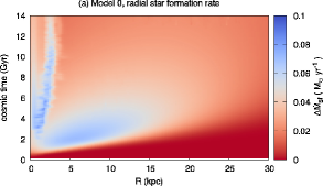
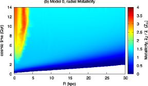
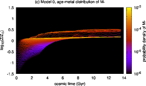
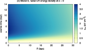
Figure 8: (a) The spacetime diagram of the radial star formation rate, $\Delta\dot{M}_{\rm sf}$. (b) The spacetime diagram of the disk gas metallicity, $\Sigma_{Z}/\Sigma$ for which $\Delta\dot{M}_{\rm sf}>10^{-8}~{}M_{\odot}~{}{\rm yr^{-1}}$. (c) The probability density distribution of the stellar metallicity for the cosmic time, corresponding to the age-metal distribution of the low-mass stars. (d) The spacetime diagram of the CR energy density at $z=0$ kpc.

Figures 8a and 8b show the spacetime diagrams of the radial star formation rate, $\Delta\dot{M}_{\rm sf}=2\pi\dot{\Sigma}_{\rm sf}R\Delta R$, and the disk gas metallicity, $\Sigma_{Z}/\Sigma$, respectively. The star formation history follows the assumed $\dot{\Sigma}_{\rm b,disk}$ given by the equation (35). At the inner radius of $R\lesssim 3$ kpc, the mass transfer by the falling-back wind particles leads to higher star formation rates. The metallicity of the disk gas becomes large at $R\lesssim 3~{}{\rm kpc}$ due to the metal transfer by the falling-back wind particles. Note that the cosmological accretion gas dose not contain the metals. The metallicity at $R\gtrsim 5$ kpc is almost constant with a value of $\sim Z_{\odot}$ over the cosmic time because of the large mass transfer rate of wind, $\dot{M}_{\rm w}\sim\dot{M}_{\rm b}$, and the small mass depletion rate of the CGM, $\dot{M}_{\rm cl}\ll\dot{M}_{\rm b}$. Most of the created metals goes to and stays in the CGM; $M_{\rm cgm}\sim 10^{11}~{}M_{\odot}$ (see, Figure 3b) and the CGM metallcity is $\sim 0.5~{}Z_{\odot}$ (see, Figure 5d). This trend of larger metallicity at the inner radius region is consistent with the current state of the Galactic disk. Figure 8c shows the age-metallicity distribution of the low-mass stars. The older stars tend to have smaller metallcities and the typical stellar metallicity is $Z_{\odot}$, which reflects the metallcity of the disk gas. Note that our model result is based on the long-term averaged argument. The actual stellar metallicity may reflect local and short time scale physical processes and conditions, which would produce a larger dispersion than our result. The mean behavior,— rapid growth at $t\lesssim 2$ Gyr and plateau distribution with $Z\sim Z_{\odot}$ at $t\gtrsim 2$ Gyr —, is similar to the observed one by Gaia satellite (Xiang & Rix (2022)) The CR energy density, $e_{\rm cr}$, shown in Figure 8d also traces the mass accretion via the star formation rate, but the structures are smoothed out by the diffusion.

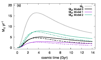
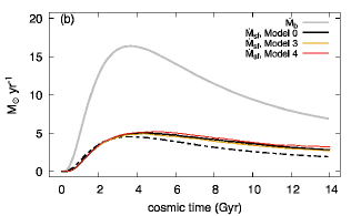
Figure 9: The results of star formation rate $\dot{M}_{\rm sf}$ for the models summarized in Table 2.3. The solid gray line, broken black line, and black lines are the same as Figure 2a and 3a. (a) The results of the strong wind case (Model 1, purple) and the weak wind case (Model 2, green). (b) The results of the large $e_{\rm cr}$ case (Model 3, orange) and the small $e_{\rm cr}$ case (Model 4, red).

Figure 9 shows the results of $\dot{M}_{\rm sf}$ for each model summarized in Table 2.3. The different conversion efficiency $\eta_{\rm blown}$ (Model 1 and 2) results in the different mass transfer rate of the outflow via $\dot{\Sigma}_{\rm blown}=\eta_{\rm w}\dot{\Sigma}_{\rm sn}\propto\eta_{\rm blown}$ and the effects of $H_{\rm cr}$ (Model 3 and 4) appear via $\dot{\Sigma}_{\rm fb}$. In the case of larger $\eta_{\rm blown}$ (Model 1, the purple lines in Figure 9a), the gaseous matter is efficiently removed by the wind and therefore the CGM mass becomes larger than in the case of Model 0. The opposite behavior is obtained in the case of smaller $\eta_{\rm blown}$ (Model 2, the green lines in Figure 9a). Such simple interpretations can also be found from the fact that the calculated $\dot{M}_{\rm sf}$ of each case is in good agreement with the estimated star formation rate given by the equation (36) for which $\dot{\Sigma}_{\rm cl}=\dot{\Sigma}_{\rm fb}=0$. For Model 1 ($\eta_{\rm blown}=0.05$), the total mass of low-mass stars is $M_{*}\simeq 6\times 10^{10}~{}M_{\odot}$. This is still consistent with the observationally estimated total stellar mass in the MW, $4\mathchar 45\relax 6\times 10^{10}~{}M_{\odot}$ (Bland-Hawthorn & Gerhard (2016)). On the other hand, for Model 2 ($\eta_{\rm blown}=0.2$), the mass is $M_{*}\simeq 2\times 10^{10}~{}M_{\odot}$, which is not likely. Figure 9b shows the larger $e_{\rm cr}$ case (Model 3, the orange line) and the smaller $e_{\rm cr}$ case (Model 4, the red line). Although the total star formation rate of each case may be acceptable, the CR energy density in the disk becomes $\sim 4\mathchar 45\relax 8~{}{\rm eV~{}cm^{-3}}$ for Model 3, which is a bit too large. In the case of Model 4, the energy density is $\sim 0.5\mathchar 45\relax 2~{}{\rm eV~{}cm^{-3}}$, which may still be acceptable. This weak dependence on $H_{\rm cr}$ implies that the Galactic evolution may be stable for variations in the CR energy density due to the uncertain magnetic field properties (or the diffusion coefficient). Note that the galactic wind solutions derived by Shimoda & Inutsuka (2022) exist in the range of $e_{\rm cr}\sim 0.1\mathchar 45\relax 10~{}{\rm eV~{}cm^{-3}}$. Thus, to reproduce the current MW, the parameter range of $0.05\lesssim\eta_{\rm blown}\lesssim 0.1$ and $10~{}{\rm kpc}\lesssim H_{\rm cr}\lesssim 14~{}{\rm kpc}$ with $\eta_{\rm cr}=0.1$ is favored.

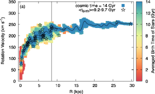
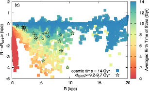
Figure 10: (a) The rotation curves at $t=14$ Gyr and $z=0$ kpc of Model 0. The gray line shows the rotation velocity calculated from the DM potential alone. The black curve shows the velocities calculated from the sum of the DM and mass components at the disk. The vertical black line indicates $R=8.5$ kpc. The square boxes are the stellar parcels and their color shows the averaged birth time, $\langle t\rangle_{\rm birth}$. The star symbols indicate parcels with $9.2~{}{\rm Gyr}<\langle t\rangle_{\rm birth}<9.7~{}{\rm Gyr}$. Note that the points of the stellar parcels overlap. (b) The distribution of stellar parcels in the velocity space. (c) The relation of stellar parcels between the current palce and averaged birth place $\langle R\rangle_{\rm birth}$.

To test the assumed $\dot{\Sigma}_{\rm b,disk}$ given by the equation (35), the rotation curve argument can be useful. Figure 10a shows the rotation velocity at $t=14$ Gyr and $z=0$ kpc. The flat rotation with a velocity of $\sim 200\mathchar 45\relax 250~{}{\rm km~{}s^{-1}}$ is well reproduced (e.g., Mróz et al. (2019), for the observed one). The dispersion of rotation curve is due to the collisionless nature of the stars. For the other models, the curves are similar to each other. Thus, we regard that the assumptions in $\dot{\Sigma}_{\rm b,disk}$ can be reasonable. Figure 10b shows the distribution of stellar parcels in the velocity space (see, Belokurov et al. (2018), for the one observed by the Gaia satellite). Note that since our model does not account for perturbations from local objects such as giant molecular clouds, the result tends to have a smaller dispersion than the realistic one. The older stars tend to be at $R\lesssim 3$ kpc and have a large radial velocity dispersion, reflecting the rapid growth of the gravitational potential in the early stage. The relatively younger stars have a smaller radial velocities with a smaller dispersion, corresponding to the Galactic stellar disk. The growth of gravitational potentail results in a systematic stellar migration which is indicated by Figure 9c. This tendency may be an indication of the bulge formation process, which will be studied in our future work.

4 Implication for Observations

We discuss the implications of our model for various observations focusing on the assumed gas accretion, the origin of the outflowing hot X-ray emitting gas, and so on.

4.1 The dark accretion flow tested by the X-ray, ultraviolet, infrared and radio observations

Finding the gas accretion flow onto the disk is important but an unsettled issue in the MW. In our model, we assume that the most of the cosmological accretion gas with a number density of $\sim 10^{-2}~{}{\rm cm^{-3}}$ falls directly onto the disk. Although the actual physical conditions of the cosmological accretion gas are non-trivial, the interactions between the dense, possibly low-temperature accretion gas and the diffuse gas in the galactic halo are important issues that may be similar to the cooling flow problem in the clusters of galaxies (Fabian (1994); Makishima et al. (2001); Peterson et al. (2003); Peterson & Fabian (2006)). If the case, observations at the soft X-ray band may be important to find the accretion flow in the analogue of the clusters of galaxies.

The high-velocity clouds and intermediate-velocity clouds observed at the Galactic halo region by the $21~{}{\rm cm}$ line emission may be part of this expected accretion gas (Wakker & van Woerden (1997); Putman et al. (2012); Hayakawa & Fukui (2022)). The estimated mass accretion rate of the observed HI components, $\sim 0.1\mathchar 45\relax 0.5~{}M_{\odot}~{}{\rm yr^{-1}}$, is too small to be responsible for the star formation rate of $\sim 3~{}M_{\odot}~{}{\rm yr^{-1}}$, although the distance of these clouds are not tightly constrained (i.e., the total mass is uncertain. See, Putman et al. (2012), and references therein). In our model, the mass accretion from the CGM region occurs with an assumed efficiency of the angular momentum transfer in condensation processes ($\epsilon_{\rm cgm}=0.01$). The accretion rate is $\dot{M}_{\rm cl}\sim 0.5~{}M_{\odot}{\rm yr^{-1}}$, which can be consistent with the estimated accretion rate of the observed HI components. Hayakawa & Fukui (2022) argued the origin of the intermediate-velocity clouds and found that a picture of the external low-metallicity HI gas accretion is favored instead of the Galactic-fountain model (Shapiro & Field (1976)). This scenario is consistent with our model results.

Thus, our model predicts the existence of dark accretion flows (DAFs) with a possible number density of $\sim 10^{-2}~{}{\rm cm^{-3}}$, corresponding to $\dot{\Sigma}_{\rm b,disk}$ given by the equation (35). The DAFs are expected to be responsible for the continuous star formation rate in the disk, and the galactic rotation curve reflects the accretion dynamics of the DAFs. When the temperature of the DAFs is comparable to the virial temperature ($\sim 10^{6}$ K), the DAFs are bright in the far ultraviolet and/or soft X-ray bands, which are actually obscured by the disk gas in the case of observations from the solar system. Investigating the dynamics of the gaseous matter including the DAFs, wind, HI clouds, and so on would be one of the most important issue. We will address this issue together with the study of the observational methods in future work.

It is worth emphasizing that an alternative scenario for the origin of DAFs is that most of the cosmological gas accretion remains in the Galactic halo or CGM region, — not accreting directly onto the disk due to the uncertain angular momentum properties. In this case, the mass accretion responsible for sustaining the long-term star formation is invoked from the metal-polluted CGM with a larger $\epsilon_{\rm cgm}$, although most of CGM gas should be virialized to explain the observed massive CGM. Then, the observational implications are changed as that the accretion gas consists of the metals and possibly dust grains produced during the gas condensation processes. The metals can produce the atomic line emissions in the ultraviolet band to the X-ray band so that the gas accretion motions can be identified by the detailed spectroscopy. The amount of dust grains is also an important predictable value that can be tested by the observations in the radio and infrared bands.

4.2 The accretaion history tested by the galactic archaeology

The relations between the stellar age, metallicity, and phase space distribution are important clues for investigating a galactic evolution. In the case of the MW, a sophisticated chemical abundance modeling favors much more episodic gas accretion onto the disk than that assumed in this paper to explain clear distinguished two sequences in [Mg/Fe] versus [Fe/H] relation (e.g., Spitoni et al. (2021); Sahlholdt et al. (2022)). The interpretation and prediction of the two sequences are not so simple because; (i) the stars can move from their birth place, (ii) the most of ejected metals should be removed from the disk by the wind, (iii) a fraction of the wind possibly falls back onto the inner disk, and (iv) (local) gas or dust migration/dynamics may affect (e.g., Chen et al. (2023)). In particular, the formation condition and migration of white dwarf(s) in a close binary system, which results in the Fe pollution by type Ia supernovae, may be significantly uncertain. Thus, it would be worth considering an another footprint for the accretion history.

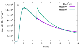
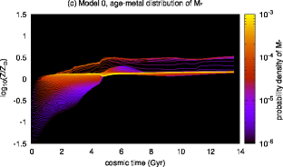
Figure 11: (a) The accretion rate onto the disk at $R=8$ kpc. The purple line indicates Model 0. The green line indicates the case of the episodic accretion. (b) The rate at $R=1$ kpc. (c) The age-metal distribution of the low-mass stars in the case of the episodic accretion. The other parameters are the same as Model 0.

To investigate the accretion history onto the disk, we adopt the episodic gas accretion scenario by replacing the term of $\exp[-(R-r_{\rm core})^{2}/2r_{\rm core}{}^{2}]$ in the equation (35) to $\exp[-(R-r_{\rm core})^{2}/2(r_{\rm core}/2){}^{2}]$ at $t>5$ Gyr, i.e., the accretion gas is more concentrated. The other parameters are the same as Model 0.

Figures 11a and 11b are the resultant gas accretion rate onto the disk at $R=8$ kpc (a) and $R=1$ kpc (b). The concentrated accretion of the primordial gas more dilutes the disk gas metallicity at $R\sim r_{\rm core}(t=5~{}{\rm Gyr})\sim 10$ kpc, while the inner radius region is less diluted. Such accretion history forms high-metallicity stars at the inner galaxy which can be seen in the age-metallicity distribution (Figure 11c). Future observations providing more complete stellar samples such as JASMINE (Gouda & Jasmine Team (2021)) will constrain the actual gas accretion history.

4.3 The origin of outflowing gas tested by X-ray observations

The gas with the virial temperature for the galactic mass scale, $kT_{\rm vir}\sim 0.1~{}{\rm keV}(M_{\rm vir}/10^{12}~{}M_{\odot})$, is bright at the X-ray band. The X-ray observations play a key role in studying the outflow from the galactic system in general.

The origin and formation processes of the diffuse X-ray emission around the Galactic disk are currently controversial issues as reviewed by Koyama (2018) for the GDXE. Note that the outflow is alternatively responsible for removing the metals from the galactic disk. Thus, a fraction of the disk gas should have a temperature of $T\gtrsim T_{\rm vir}$ to transfer the metals from the disk to the Galactic halo region. In our model, we assume that the outflows are driven by consuming a tenth of the supernova explosion energy ($\eta_{\rm blown}\sim 0.1$). The proposed candidates for the GDXE origin(s) are the assembly of young-intermediate-aged supernova remnants and/or discrete, unresolved stellar objects. The former scenario is possibly consistent with the numerical simulation results of the local galactic disk performed by Girichidis et al. (2018), although the current computational resources are far from sufficient to resolve the energy injection processes by the supernovae in general. It is worth pointing out that the CRs are also able to heat the diffuse gas via the dissipation of self-excited Alfvén waves at a rate comparable to the radiative cooling rate as discussed by Shimoda & Inutsuka (2022). Note that Shimoda & Inutsuka (2022) assumed one of the simplest CR heating scenarios (e.g., Volk & McKenzie (1981); Zirakashvili et al. (1996)), but the effects of the CR heating on the background plasma remain to be studied (e.g., Zweibel (2020); Yokoyama & Ohira (2023)). Thus, further investigations on the origin of GDXE are necessary for the understanding of the Galactic long-term evolution and these are the science cases of future X-ray observations such as XRISM (Tashiro et al. (2020)), and Athena (Nandra et al. (2013)).

Related to the origin of the GDXE, the galactic center activity is potentially important (e.g., Totani (2006); Koyama (2018)). Note that the galactic center of our galaxy roughly corresponds to the region around Sgr A^∗ within a radius of $\sim 300$ pc. This region is not resolved by our model. The existence of such activities is also favored to explain the bubble-like structures seen in the soft X-ray sky (e.g., Predehl et al. (2020)) and possibly smaller bubble structures bright at the $\gamma$-ray band (the so-called Fermi bubble, Su et al. (2010), but see also Crocker et al. (2022) suggesting the externalgalaxy scenario). The effects of such activities are not considered in our model and are also important issues for the net gas accretion rate at the Galactic center, which is related to the formation and evolution process of the supermassive black hole.

The outflow originated from the disk may explain the metal pollution of the CGM as we mentioned in this paper. The actual CGM temperature is also important to understand the observed ‘stable’ CGM (e.g., Miller & Bregman (2015); Tumlinson et al. (2017); Nakashima et al. (2018); Das et al. (2019)). If the temperature of CGM was much smaller than the virial temperature of $\sim 10^{6}$ K, a significant gas accretion from the CGM would happen. In the case of the MW, the estimated mass and temperature are $\sim 4\times 10^{10}~{}M_{\odot}$ and $\sim 3\times 10^{6}$ K, respectively (Miller & Bregman (2015)). Das et al. (2019) reported that a very hot phase with temperature of $\sim 10^{7}$ K is possibly co-spatial in the CGM. In the case of external galaxies, lower-ionized ions are also reported (Tumlinson et al. (2017)). Shimoda & Inutsuka (2022) studied the Galactic wind theoretically and showed that the allowed wind solutions range from $10^{4}$ K to $10^{7}$ K depending on the physical conditions (especially, the CR pressure) at the hot gas layer ($z\sim 2$ kpc). Obviously, the angular momentum distribution is also important however it is more uncertain than the thermal condition. Further theoretical and observational investigations of the thermal condition, chemical enrichment, and angular momentum distribution of the CGM are necessary.

4.4 Implication for the planet formation and cosmic life

The amounts of metals and CRs in the disk are important for the planet formation. The protoplanetary disk (PPD) can be quickly dissipated by too efficient angular momentum transport in the ideal magnetohydrodynamics regime, so the effects of finite magnetic resistivity are invoked for long-lived PPDs (e.g., Inutsuka (2012); Tsukamoto et al. (2022), for reviews). The magnetic resistivity is, however, uncertain due to large uncertainties in the CR ionization rate, the amount of the dust, and the dust size distributions (e.g., Tsukamoto & Okuzumi (2022)). Further development along the lines of this study such as the dust formation and detailed CR transport in the disk would describe the change due to the Galactic evolution for the environment of PPDs in terms of the amount of dust and CRs over cosmic time as shown in Figures 8b and 8d, and provide a useful step for investigations of the birthplace of the solar system. We will attempt to extend our model in future work.

The almost constant star formation rate of $\sim M_{\odot}~{}{\rm yr^{-1}}$ corresponds to the almost constant supernova rates under the assumption of the universal initial mass function and star formation efficiency, $\epsilon_{\rm sf}$. In contrast, the size of the gas disk can evolve in time from the center to outward, reflecting the gas accretion. Thus, the star and planet systems formed at a very early cosmic time, say $t<2$ Gyr, are more frequently swept up by the supernova blast waves than those formed at later times. The irradiation of the CRs and high-energy photons is also strong at the early time. It may be more severe conditions for cosmic life to survive than the current condition. The frequent shock propagation may also affect the dust grains in the ISM. At $t\sim 4$ Gyr, the size evolution of the gas disk almost converges (Figure 4b), and the local star formation rate starts to increase at $R\lesssim 3$ kpc (gradually decreasing at $R\gtrsim 3$ kpc, Figure 8a). These are interesting clues to study the habitable region and time of the Galactic disk.

4.5 Further improvement by observations of externalgalaxies

The comparison with the observations of externalgalaxies will also provide improvement of our modeling. Since our model can simultaneously describe the star formation history, CR energy density, metallicity, and total baryon mass of galactic halo, the correlations among the galaxy color magnitude diagram, $\gamma$-ray luminosity, and neutrino luminosity can be studied in a self-consistent manner. The origin of high-energy cosmic neutrinos discovered by the IceCube Collaboration (Aartsen et al. (2013); IceCube Collaboration (2013)) is considered as a possible evidence for the existence of hidden CR accelerators (e.g., Murase (2022)). Our model is also useful for studying such a big enigma in particle astrophysics.

The difference and relation between the host galaxy and its satellites would also be interesting subjects. Ruiz-Lara et al. (2020) suggested that repeated encounters of the Sagittarius dwarf galaxy with the MW result in star formation enhancements in the past of $\sim 5.7$ Gyr, $1.9$ Gyr, and $1.0$ Gyr ago. We will investigate what insights can be obtained from such multimessenger astronomy methods, including the effects from satellites in future work.

Once we have a reasonable model for Galaxy evolution, we may predict the future of our Galaxy (see, e.g., Tutukov et al. (2000)). For example, according to a simple extrapolation we need  100 Gyr to make the mean metallicity on the order of 10%, which might be too large to test observationally. However, it might not be impossible to study the effect of such a large metallicity by the systematic observation of the extreme regions in some external galaxies.

5 Summary

We have constructed the model of the Galactic system that describes the long-term evolution of the star formation, CRs, metallicity, and stellar dynamics over cosmic time. The Galactic gas disk can be modeled by the accretion disk with the $\alpha$ prescription however the radial mass transfer is not so important for the surface mass density profiles due to the limited amount of turbulent radial excursion of the gas. This can be easily understood by $\alpha/C_{s}{}^{2}<0.1$ and $10~{}{\rm kpc}/C_{s}\sim 1~{}{\rm Gyr}\left(C_{s}/10~{}{\rm km~{}s^{-1}}\right)$ that corresponds to the sound crossing time of the gas at $10^{4}$ K, which is essentially determined by the Ly$\alpha$ cooling. When the galactic wind is driven, the long-term star formation can be simply estimated by the equation (16). Considering the consistency between the observed diffuse X-ray emission of the current MW (Koyama, 2018; Nakashima et al., 2018; Predehl et al., 2020) and the steady-state wind solutions given by Shimoda & Inutsuka (2022), we have found that if about a tenth of the supernova explosion energy is consumed to form such diffuse, hot X-ray emitting gas (i.e., $\eta_{\rm blown}\sim 0.1$), the star formation rate of a few $M_{\odot}~{}{\rm yr^{-1}}$ can be explained. This hypothesis will be investigated by future X-ray missions; XRISM, Athena, and so on. We have found that the acceptable CR energy density of a few ${\rm eV~{}cm^{-3}}$ in the disk given by the CR scale height of $H_{\rm cr}\sim 10$ kpc can explain the long-term star formation rate. In our model, a fraction of the wind mass falls back to the disk. The mass transfer rate of the falling-back wind is a minor component of the net accretion rate of the total gas mass as a result, while it is responsible for the metallicity increase of the disk gas in the inner radius region (see, Figure 8b). To test the validity of our scenario in particular the assumed accretion rate of the disk given by the equation (35), we have estimated the rotation curves of the low-mass stars and found that the parameter set of $(\eta_{\rm blown};H_{\rm cr})=(0.1,10~{}{\rm kpc})$ can simultaneously explain the star formation rate, metallicity in the disk, CR energy density in the disk, and the rotation curve.

We thank T. Ishiyama, S. Inoue, M. Nobukawa, K. Nobukawa, S. Yamauchi, T. G. Tsuru, D. Kashino, and S. Cooray, for useful discussions and suggestions. We are grateful to the anonymous referee, for his/her comments that further improved the paper. This work is partly supported by JSPS Grants-in-Aid for Scientific Research Nos. 20J01086 (JS), 18H05436, 18H05437 (SI), and 20H01950 (MN).

References

- Aartsen et al. (2013) Aartsen, M. G., Abbasi, R., Abdou, Y., et al. 2013, Phys. Rev. Lett., 111, 021103
- Asplund et al. (2009) Asplund, M., Grevesse, N., Sauval, A. J., & Scott, P. 2009, ARA&A, 47, 481
- Balbus & Hawley (1998) Balbus, S. A., & Hawley, J. F. 1998, Reviews of Modern Physics, 70, 1
- Belokurov et al. (2018) Belokurov, V., Erkal, D., Evans, N. W., Koposov, S. E., & Deason, A. J. 2018, MNRAS, 478, 611
- Bland-Hawthorn & Gerhard (2016) Bland-Hawthorn, J., & Gerhard, O. 2016, ARA&A, 54, 529
- Chandrasekhar (1943) Chandrasekhar, S. 1943, ApJ, 97, 255
- Chen et al. (2023) Chen, B., Hayden, M. R., Sharma, S., et al. 2023, MNRAS, 523, 3791
- Chieffi & Limongi (2020) Chieffi, A., & Limongi, M. 2020, ApJ, 890, 43
- Crocker et al. (2022) Crocker, R. M., Macias, O., Mackey, D., et al. 2022, Nature Astronomy, 6, 1317
- Cummings et al. (2016) Cummings, A. C., Stone, E. C., Heikkila, B. C., et al. 2016, ApJ, 831, 18
- Das et al. (2019) Das, S., Mathur, S., Nicastro, F., & Krongold, Y. 2019, ApJ, 882, L23
- Evoli et al. (2020) Evoli, C., Morlino, G., Blasi, P., & Aloisio, R. 2020, Phys. Rev. D, 101, 023013
- Fabian (1994) Fabian, A. C. 1994, ARA&A, 32, 277
- Fujimoto et al. (2023) Fujimoto, Y., Inutsuka, S.-i., & Baba, J. 2023, MNRAS, arXiv:2305.07050
- Gabici et al. (2019) Gabici, S., Evoli, C., Gaggero, D., et al. 2019, International Journal of Modern Physics D, 28, 1930022
- Girichidis et al. (2018) Girichidis, P., Naab, T., Hanasz, M., & Walch, S. 2018, MNRAS, 479, 3042
- Gnat (2017) Gnat, O. 2017, ApJS, 228, 11
- Gouda & Jasmine Team (2021) Gouda, N., & Jasmine Team. 2021, in Astronomical Society of the Pacific Conference Series, Vol. 528, New Horizons in Galactic Center Astronomy and Beyond, ed. M. Tsuboi & T. Oka, 163
- Hayakawa & Fukui (2022) Hayakawa, T., & Fukui, Y. 2022, arXiv e-prints, arXiv:2208.13406
- Haywood et al. (2016) Haywood, M., Lehnert, M. D., Di Matteo, P., et al. 2016, A&A, 589, A66
- Hennebelle & Inutsuka (2019) Hennebelle, P., & Inutsuka, S.-i. 2019, Frontiers in Astronomy and Space Sciences, 6, 5
- Hodges-Kluck et al. (2020) Hodges-Kluck, E. J., Yukita, M., Tanner, R., et al. 2020, ApJ, 903, 35
- IceCube Collaboration (2013) IceCube Collaboration. 2013, Science, 342, 1242856
- Inoue & Inutsuka (2009) Inoue, T., & Inutsuka, S.-i. 2009, ApJ, 704, 161
- Inoue & Inutsuka (2012) —. 2012, ApJ, 759, 35
- Inutsuka (2012) Inutsuka, S.-i. 2012, Progress of Theoretical and Experimental Physics, 2012, 01A307
- Inutsuka et al. (2015) Inutsuka, S.-i., Inoue, T., Iwasaki, K., & Hosokawa, T. 2015, A&A, 580, A49
- Kennicutt & Evans (2012) Kennicutt, R. C., & Evans, N. J. 2012, ARA&A, 50, 531
- Koyama (2018) Koyama, K. 2018, PASJ, 70, R1
- Krough et al. (1982) Krough, F. T., Ng, E. W., & Snyder, W. V. 1982, Celestial Mechanics, 26, 395
- Lass & Blitzer (1983) Lass, H., & Blitzer, L. 1983, Celestial Mechanics, 30, 225
- Makishima et al. (2001) Makishima, K., Ezawa, H., Fukuzawa, Y., et al. 2001, PASJ, 53, 401
- Miller & Bregman (2015) Miller, M. J., & Bregman, J. N. 2015, ApJ, 800, 14
- Mróz et al. (2019) Mróz, P., Udalski, A., Skowron, D. M., et al. 2019, ApJ, 870, L10
- Murase (2022) Murase, K. 2022, ApJ, 941, L17
- Naab & Ostriker (2017) Naab, T., & Ostriker, J. P. 2017, ARA&A, 55, 59
- Nakashima et al. (2018) Nakashima, S., Inoue, Y., Yamasaki, N., et al. 2018, ApJ, 862, 34
- Nandra et al. (2013) Nandra, K., Barret, D., Barcons, X., et al. 2013, arXiv e-prints, arXiv:1306.2307
- Navarro et al. (1996) Navarro, J. F., Frenk, C. S., & White, S. D. M. 1996, ApJ, 462, 563
- Navarro et al. (1997) —. 1997, ApJ, 490, 493
- Peterson & Fabian (2006) Peterson, J. R., & Fabian, A. C. 2006, Phys. Rep., 427, 1
- Peterson et al. (2003) Peterson, J. R., Kahn, S. M., Paerels, F. B. S., et al. 2003, ApJ, 590, 207
- Pfrommer et al. (2017) Pfrommer, C., Pakmor, R., Schaal, K., Simpson, C. M., & Springel, V. 2017, MNRAS, 465, 4500
- Pineda et al. (2022) Pineda, J. E., Arzoumanian, D., André, P., et al. 2022, arXiv e-prints, arXiv:2205.03935
- Planck Collaboration et al. (2020) Planck Collaboration, Aghanim, N., Akrami, Y., et al. 2020, A&A, 641, A6
- Posti & Helmi (2019) Posti, L., & Helmi, A. 2019, A&A, 621, A56
- Predehl et al. (2020) Predehl, P., Sunyaev, R. A., Becker, W., et al. 2020, Nature, 588, 227
- Putman et al. (2012) Putman, M. E., Peek, J. E. G., & Joung, M. R. 2012, ARA&A, 50, 491
- Rodríguez-Puebla et al. (2016) Rodríguez-Puebla, A., Behroozi, P., Primack, J., et al. 2016, MNRAS, 462, 893
- Ruiz-Lara et al. (2020) Ruiz-Lara, T., Gallart, C., Bernard, E. J., & Cassisi, S. 2020, Nature Astronomy, 4, 965
- Sahlholdt et al. (2022) Sahlholdt, C. L., Feltzing, S., & Feuillet, D. K. 2022, MNRAS, 510, 4669
- Shakura & Sunyaev (1973) Shakura, N. I., & Sunyaev, R. A. 1973, A&A, 24, 337
- Shapiro & Field (1976) Shapiro, P. R., & Field, G. B. 1976, ApJ, 205, 762
- Shimoda & Inutsuka (2022) Shimoda, J., & Inutsuka, S.-i. 2022, ApJ
- Shimoda et al. (2022) Shimoda, J., Ohira, Y., Bamba, A., et al. 2022, PASJ
- Sofue (2012) Sofue, Y. 2012, PASJ, 64, 75
- Spitoni et al. (2021) Spitoni, E., Verma, K., Silva Aguirre, V., et al. 2021, A&A, 647, A73
- Su et al. (2010) Su, M., Slatyer, T. R., & Finkbeiner, D. P. 2010, ApJ, 724, 1044
- Sukhbold et al. (2018) Sukhbold, T., Woosley, S. E., & Heger, A. 2018, ApJ, 860, 93
- Suzuki & Inutsuka (2009) Suzuki, T. K., & Inutsuka, S.-i. 2009, ApJ, 691, L49
- Suzuki et al. (2010) Suzuki, T. K., Muto, T., & Inutsuka, S.-i. 2010, ApJ, 718, 1289
- Suzuki et al. (2016) Suzuki, T. K., Ogihara, M., Morbidelli, A., Crida, A., & Guillot, T. 2016, A&A, 596, A74
- Tashiro et al. (2020) Tashiro, M., Maejima, H., Toda, K., et al. 2020, in Society of Photo-Optical Instrumentation Engineers (SPIE) Conference Series, Vol. 11444, Society of Photo-Optical Instrumentation Engineers (SPIE) Conference Series, 1144422
- Totani (2006) Totani, T. 2006, PASJ, 58, 965
- Tsukamoto & Okuzumi (2022) Tsukamoto, Y., & Okuzumi, S. 2022, ApJ, 934, 88
- Tsukamoto et al. (2022) Tsukamoto, Y., Maury, A., Commerçon, B., et al. 2022, arXiv e-prints, arXiv:2209.13765
- Tumlinson et al. (2017) Tumlinson, J., Peeples, M. S., & Werk, J. K. 2017, ARA&A, 55, 389
- Tutukov et al. (2000) Tutukov, A. V., Shustov, B. M., & Wiebe, D. S. 2000, Astronomy Reports, 44, 711
- van der Kruit & Freeman (2011) van der Kruit, P. C., & Freeman, K. C. 2011, ARA&A, 49, 301
- Vink et al. (2006) Vink, J., Bleeker, J., van der Heyden, K., et al. 2006, ApJ, 648, L33
- Volk & McKenzie (1981) Volk, H. J., & McKenzie, J. F. 1981, in International Cosmic Ray Conference, Vol. 9, International Cosmic Ray Conference, 246–249
- Wada & Norman (2001) Wada, K., & Norman, C. A. 2001, ApJ, 547, 172
- Wakker & van Woerden (1997) Wakker, B. P., & van Woerden, H. 1997, ARA&A, 35, 217
- Watkins et al. (2023) Watkins, E. J., Barnes, A. T., Henny, K., et al. 2023, ApJ, 944, L24
- Xiang & Rix (2022) Xiang, M., & Rix, H.-W. 2022, Nature, 603, 599
- Yokoyama & Ohira (2023) Yokoyama, S. L., & Ohira, Y. 2023, MNRAS, 523, 3671
- Zirakashvili et al. (1996) Zirakashvili, V. N., Breitschwerdt, D., Ptuskin, V. S., & Voelk, H. J. 1996, A&A, 311, 113
- Zucker et al. (2022) Zucker, C., Goodman, A. A., Alves, J., et al. 2022, Nature, 601, 334
- Zweibel (2020) Zweibel, E. G. 2020, ApJ, 890, 67