Beamfocusing Optimization for Near-Field Wideband Multi-User Communications

Abstract

A near-field wideband communication system is studied, wherein a base station (BS) employs an extremely large-scale antenna array (ELAA) to serve multiple users situated within its near-field region. To facilitate the near-field beamfocusing and mitigate the wideband beam split, true-time delayer (TTD)-based hybrid beamforming architectures are employed at the BS. Apart from the fully-connected TTD-based architecture, a new sub-connected TTD-based architecture is proposed for enhancing energy efficiency. Three wideband beamfocusing optimization approaches are proposed to maximize spectral efficiency for both architectures. 1) Fully-digital approximation (FDA) approach: In this approach, the TTD-based hybrid beamformers are optimized to approximate the optimal fully-digital beamformers using block coordinate descent. 2) Penalty-based FDA approach: In this approach, the penalty method is leveraged in the FDA approach to guarantee the convergence to a stationary point of the spectral maximization problem. 3) Heuristic two-stage (HTS) approach: In this approach, the closed-form TTD-based analog beamformers are first designed based on the outcomes of near-field beam training and the piecewise-near-field approximation. Subsequently, the low-dimensional digital beamformer is optimized using knowledge of the low-dimensional equivalent channels, resulting in reduced computational complexity and channel estimation complexity. Our numerical results unveil that 1) the proposed approaches effectively eliminate the near-field beam split effect, and 2) compared to the fully-connected architecture, the proposed sub-connected architecture exhibits higher energy efficiency and imposes fewer hardware limitations on TTDs and system bandwidth.

I Introduction

Given the significantly higher performance target than the current wireless network, the sixth-generation (6G) wireless network is anticipated to incorporate two emerging trends: extremely large-scale antenna arrays (ELAAs) and significantly higher frequencies [1]. On the one hand, ELAAs are capable of realizing a large array gain and high spatial resolution, thereby improving network capacity and connectivity. On the other hand, high-frequency bands, such as millimeter-wave (mmWave) and terahertz (THz) bands, can provide enormous bandwidth resources to advance network performance. Nonetheless, the evolution towards ELAAs and the utilization of mmWave or THz frequency bands not only entails an increase in the number of antennas and carrier frequencies but also brings about significant modifications in the electromagnetic properties of the wireless environment. In particular, the electromagnetic field region surrounding transmit antennas can be categorized into two distinct regions: the near-field region and the far-field region [2]. The Rayleigh distance, which is proportional to the aperture of the antenna array and the carrier frequency, serves as a commonly employed metric for establishing the demarcation between the near-field and far-field regions. [2]. In previous generations of wireless networks, the Rayleigh distance was typically less than a few meters. Hence, the near-field region was negligible, allowing wireless networks to be designed based on the far-field approximation. However, with the emergence of ELAAs and high frequencies, the Rayleigh distance has grown significantly, ranging from tens to even hundreds of meters [3]. Consequently, the near-field region becomes dominant in the 6G wireless network, necessitating a redesign of the wireless network under the near-field assumption.

I-A Prior Works

The fundamental changes in electromagnetic characteristics in the near-field region present new opportunities for 6G wireless communications. In far-field communications, the signal wavefront is approximated as planar, allowing for far-field beamforming that resembles a flashlight, steering the beam towards the intended direction of users [4]. Such a beamforming approach is known as far-field beamsteering. Conversely, near-field communications require a more precise spherical wavefront model. As a result, near-field beamforming acts like a spotlight and is capable of focusing the beam around user locations, which is referred to as near-field beamfocusing [3]. In contrast to far-field beamsteering, near-field beamfocusing encompasses not only the direction but also the distance between the base station (BS) and the users, offering additional degrees of freedom (DoFs) to enhance system capacity and reduce inter-user interference [5, 6, 7, 8, 9]. In particular, the authors of [5] analyzed the performance of near-field multi-user communications using three typical beamforming strategies. Their analysis demonstrated that the new distance dimension in near-field communications enables effective suppression of inter-user interference, even if the users are in the same direction. Instead of exploiting these typical beamforming strategies, the authors of [6] took a different approach by optimizing the beamformers specifically for various hybrid beamforming antenna architectures, in order to achieve an optimal near-field beamfocusing strategy. As a further advance, the achievable rate of near-field communications is characterized in [7] based on the circuit theory, which provides an upper bound of the system performance. The authors of [8] unveiled the significant performance loss caused by the utilization of far-field approximation by analyzing the channel gain and interference gain. Their findings underscore the critical need to transition towards near-field communications in the high-frequency bands. Most recently, the exploitation of evanescent waves in the reactive near-field region for providing extra DoFs was investigated in [9].

However, the previous studies have primarily focused on narrowband systems, neglecting the unique challenges posed by wideband systems. In wideband systems, apart from the frequency-selective effect, there exists an intrinsic spatial-selective effect, which is also known as the spatial-wideband effect, particularly for ELAAs [10]. This effect gives rise to substantial frequency-dependent channels, further complicating the behavior and performance of the wireless system. On the other hand, hybrid analog and digital beamforming architectures have emerged as the dominant choice for ELAAs in high-frequency bands due to the exorbitant power consumption and hardware cost associated with fully-digital architectures. However, the conventional hybrid beamforming architectures, which rely on phase shifters (PSs), are restricted to achieving frequency-independent beamforming due to inherent hardware limitations associated with PSs [11]. As a result, employing conventional hybrid beamforming architectures in wideband systems causes the beam split effect in the frequency domain [12, 13, 14, 15, 16, 17]. More specifically, the beams generated by analog beamformers at most subcarriers are offset from the target user, leading to substantial performance degradation. To combat the beam split effect in wideband communications, the authors of [14, 15, 16, 17] exploit true-time delayers (TTDs) in the analog beamformer. Different from PSs, TTDs introduce specific time delays to the signal, enabling them to achieve frequency-dependent phase shifts. Capitalizing on this distinctive feature of TTDs, recent studies such as [14] and [15] have proposed a TTD-based hybrid beamforming architecture that incorporates a limited number of TTDs alongside a larger number of PSs. It was demonstrated that this architecture can achieve a close performance to the fully-digital beamformer in far-field communications. To further reduce energy consumption and hardware complexity, the authors of [16] exploited the low-cost TTDs with fixed time delays. Furthermore, the optimization of time delays of TTDs was studied in [17] in the context of simultaneously transmitting and reflecting reconfigurable intelligent surfaces, where a quasi-Newton method-based algorithm was proposed.

So far, there are only a limited number of works that studied the beam split effect in near-field communications [18, 19, 20]. Specifically, the authors of [18] developed a beamforming design that utilizes spatial coding to address the near-field beam split effect for the conventional hybrid beamformer architecture. Adopting the TTD-based hybrid beamforming architecture, a heuristic beamforming design was proposed in [19] based on piecewise-far-field approximation. As a further advance, a deep-learning-based beamforming method was conceived in [20] to maximize the array gain at a single user across all subcarriers.

I-B Motivations and Contributions

In comparison to the far-field beam split effect, the near-field beam split effect presents greater challenges in beamforming design due to its dependence on both the angle and distance between the transmitter and receiver. Although there have been a few works on this topic, they primarily focus on single-user near-field communications, where the beamformers can be designed simply to maximize the array gain. However, these designs may not be suitable for multi-user communications. Hence, it is still an open question that how close the performance of TTD-based hybrid beamforming architecture is to the optimal fully-digital one in near-field wideband multi-user communications. Furthermore, there is still a lack of studies on beamforming design specifically for the sub-connected TTD-based hybrid beamforming architecture in the literature. Hence, the objective of this paper is to explore the beamforming design for near-field wideband multi-user communications, focusing on both fully-connected and sub-connected TTD-based hybrid beamforming architectures. The primary contributions of this paper can be succinctly summarized as follows:

• We propose a new sub-connected TTD-based hybrid beamforming architecture. This architecture achieves a remarkable reduction in the number of PSs, while only requiring a few TTDs to effectively mitigate the near-field beam split effect. Then, we formulate the spectral efficiency maximization problems for both the fully-connected and sub-connected architectures.

• We first propose fully-digital approximation (FDA) approach to maximize the spectral efficiency. In this approach, the TTD-based hybrid beamformer is optimized to approximate the optimal fully-digital beamformer. For the fully-connected architecture, we proposed a block coordinate descent (BCD)-based algorithm to solve the FDA optimization problem. For the sub-connected architecture, by exploiting the special sub-connected structure of the hybrid beamformer, we propose a BCD-based algorithm with reduced complexity. Based on the FDA approach, we further develop a penalty-based FDA approach, which ensures the convergence to a stationary point of the spectral efficiency maximization problem.

• We then propose a low-complexity heuristic two-stage (HTS) approach. In this approach, we begin by deriving a closed-form design of analog beamformers realized by PSs and TTDs based on a piecewise-near-field approximation of the line-of-sight (LoS) near-field channels. Subsequently, we optimize the low-dimensional digital beamformer using the low-dimensional equivalent channels. The HTS approach significantly reduces the channel estimation overhead, as it only requires knowledge of the LoS channels, which can be obtained by near-field beam training, and the low-dimensional equivalent channels.

• Our numerical results unveil that 1) the near-field beam split effect can be effectively eliminated by leveraging TTDs; 2) the penalty-based FDA approach yields the best performance for fully-connected and sub-connected architectures, while the FDA-only approach demonstrates comparatively lower efficiency, particularly in the case of the sub-connected architecture; 3) the HTS approach can attain a comparable performance to the penalty-based FDA approach; and 4) compared to the fully-connected architecture, the sub-connected architecture achieves higher energy efficiency by reducing the number of PSs and TTDs.

I-C Organization and Notations

The remainder of this paper is organized as follows. Section II presents the system model and formulates the wideband beamfocusing optimization problem. Sections III and IV provide the details of the proposed FDA and penalty-based PDA approaches, respectively, while the details of the proposed HTS approach are presented in Section V. Section VI demonstrates the numerical results. Section VII concludes this paper.

Notations: Scalars, vectors, and matrices are represented by the lower-case, bold-face lower-case, and bold-face upper-case letters, respectively; The transpose, conjugate transpose, pseudo-inverse, and trace of a matrix are denoted by $\mathbf{X}^{T}$, $\mathbf{X}^{H}$, $\mathbf{X}^{\dagger}$, and $\mathrm{tr}(\mathbf{X})$, respectively. The Euclidean norm of vector $\mathbf{x}$ is denoted as $\|\mathbf{x}\|$, while the Frobenius norm of matrix $\mathbf{X}$ is denoted as $\|\mathbf{X}\|_{F}$. For matrix $\mathbf{X}$, $[\mathbf{X}]_{i,j}$ refers to its entry in the $i$-th row and $j$-th column. $[\mathbf{X}]_{i:j,:}$ represents a matrix composed of the rows from the $i$-th to the $j$-th, and $[\mathbf{X}]_{:,i}$ represents a vector composed of the $i$-th column. For vector $\mathbf{x}$, $[\mathbf{x}]_{i:j,:}$ indicates a vector containing the entries from the $i$-th to the $j$-th. A block diagonal matrix with diagonal blocks $\mathbf{x}_{1},\dots,\mathbf{x}_{N}$ is denoted as $\mathrm{blkdiag}(\mathbf{x}_{1},\dots,\mathbf{x}_{N})$. $\mathbb{E}[\cdot]$ represents the statistical expectation, while $\mathrm{Re}\{\cdot\}$ refers to the real component of a complex number. $\mathcal{CN}(\mu,\sigma^{2})$ denotes the circularly symmetric complex Gaussian random distribution with mean $\mu$ and variance $\sigma^{2}$. The matrix $\mathbf{I}_{N}$ denotes the identity matrix of size $N$. The symbol $\angle$ represents the phase of a complex value.

II System Model and Problem Formulation

We consider a near-field wideband multi-user communication system in which a BS utilizes a uniform linear array (ULA) consisting of $N$ antenna elements with an antenna spacing of $d$. The system involves $K$ communication users, each equipped with a single antenna, and their indices are collected in the set $\mathcal{K}$. To mitigate inter-symbol interference inherent in wideband communications, orthogonal frequency division multiplexing (OFDM) is employed, where the signal is generated in the frequency domain and then transformed into the time domain by inverse fast Fourier transform (IFFT). Let $M$ denote the number of subcarriers in OFDM, $B$ denote the system bandwidth, $f_{c}$ denote the central carrier frequency, $c$ denote the speed of light, and $\lambda_{c}=c/f_{c}$ denote the wavelength of the central carrier. Consequently, the frequency of subcarrier $m$ is determined as $f_{m}=f_{c}+\frac{B(2m-1-M)}{2M},\forall m\in\mathcal{M}=\{1,...,M\}$.

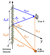
Figure 1: Illustration of the multipath near-field channel model.

II-A Near-Field Wideband Channel Model

We assume that all users are located in the near-field region of the BS, i.e., the distances between users and the BS are less than the Rayleigh distance $2D^{2}/\lambda_{c}$ [3], where $D=(N-1)d$ denotes the aperture of the antenna array. Therefore, as shown in Fig. 1, we adopt the multipath near-field channel model for each communication user, which consists of a line-of-sight (LoS) channel and several non-line-of-sight (NLoS) channels induced by $L_{k}$ scatterers associated with user $k$. We first focus on the user $k$. The distance and angle of the user with respect to the central element of the ULA are denoted by $\nu_{k}$ and $\theta_{k}$, respectively. By setting the origin of the coordinate system as the center of the ULA, the coordinates of the user and the $n$-th antenna element of the ULA, $\forall n\in\{0,\dots,N-1\}$ are given by $\mathbf{r}_{k}=[\nu_{k}\cos\theta_{k},\nu_{k}\sin\theta_{k}]^{T}$ and $\mathbf{s}_{n}=[\chi_{N}^{(n)}d,0]^{T}$, respectively, where $\chi_{N}^{(n)}=n-\frac{N-1}{2}$. The propagation distance of the signal from the $n$-th antenna element to the user $k$ can be calculated as follows:

$$\nu_{k,n}=\|\mathbf{r}_{k}-\mathbf{s}_{n}\|=\sqrt{\nu_{k}^{2}+(\chi_{N}^{(n)})^{2}d^{2}-2\nu_{k}\chi_{N}^{(n)}d\cos\theta_{k}}.$$ (1)

Similarly, the coordinate of the $l$-th scatterer for user $k$ is given by $\tilde{\mathbf{r}}_{k,l}=[\tilde{\nu}_{k,l}\cos\tilde{\theta}_{k,l},\tilde{\nu}_{k,l}\sin\tilde{\theta}_{k,l}]^{T}$, where $\tilde{\nu}_{k,l}$ and $\tilde{\theta}_{k,l}$ denote the distance and angle of the $l$-th scatterer with respect to the central element of the ULA, respectively. Let $\bar{\nu}_{k,l}$ denote the distance between the $l$-th scatterer and user $k$. Then, the propagation distance of the single from the $n$-th element to the user $k$ through the $l$-th scatterer is given by

$$\bar{\nu}_{k,l}+\tilde{\nu}_{k,n,l}=\bar{\nu}_{k,l}+\|\tilde{\mathbf{r}}_{k,l}-\mathbf{s}_{n}\|$$

$$=\bar{\nu}_{k,l}+\sqrt{\nu_{k,l}^{2}+(\chi_{N}^{(n)})^{2}d^{2}-2\nu_{k,l}\chi_{N}^{(n)}d\cos\theta_{k,l}}.$$ (2)

Then, the baseband frequency-domain channel between the user and the $n$-th antenna element for the subcarrier frequency $f_{m}$ is given by

$$h_{k,n}(f_{m})=\bar{\beta}_{k}e^{-j\frac{2\pi f_{m}}{c}\nu_{k,n}}+\sum_{l=1}^{L_{k}}\tilde{\bar{\beta}}_{k,l}e^{-j\frac{2\pi f_{m}}{c}\tilde{\nu}_{k,n,l}},$$ (3)

where $\bar{\beta}_{k}$ is the channel gain of the LoS channel, $\tilde{\bar{\beta}}_{k,l}$ is the complex channel gain of the $l$-th NLoS channel. In particular, $\bar{\beta}_{k}$ is mainly determined by the free-space pathloss while $\tilde{\bar{\beta}}_{k,l}$ involves both the free-space pathloss and the complex reflection coefficient. By stacking the channels of all antenna elements into a vector, the following overall near-field channel for subcarrier $m$ for user $k$ can be obtained:

$$\mathbf{h}_{m,k}=[h_{k,-\tilde{N}}(f_{m}),...,h_{k,\tilde{N}}(f_{m})]^{H}$$

$$=\beta_{m,k}^{*}\mathbf{b}_{N}^{*}(f_{m},\theta_{k},\nu_{k})+\sum_{l=1}^{L_{k}}\tilde{\beta}_{k,m,l}^{*}\mathbf{b}_{N}^{*}(f_{m},\tilde{\theta}_{k,l},\tilde{\nu}_{k,l}),$$ (4)

where $\mathbf{b}_{N}(f,\theta,\nu)$ is the near-field array response vector and $\tilde{\beta}_{m,k}=\bar{\beta}_{k}e^{-j\frac{2\pi f_{m}}{c}\nu_{k}}$ and $\tilde{\beta}_{k,l}=\tilde{\bar{\beta}}_{k,l}e^{-j2\pi\frac{f_{m}}{c}(\bar{\nu}_{k,l}+\tilde{\nu}_{k,l})}$ are the equivalent complex channel gains. Vector $\mathbf{b}_{N}(f,\theta,\nu)$ is given by

$$\mathbf{b}_{N}(f,\theta,\nu)=[e^{-j\frac{2\pi f}{c}(\nu_{N}^{(0)}-\nu)},\dots,e^{-j\frac{2\pi f}{c}(\nu_{N}^{(N-1)}-\nu)}]^{T},$$ (5)

where $\nu_{N}^{(n)}=\sqrt{\nu^{2}+(\chi_{N}^{(n)})^{2}d^{2}-2\nu\chi_{N}^{(n)}d\cos\theta}$. It is worth noting that the near-field array response vector is frequency-dependent. This property introduces additional challenges for the system design for near-field wideband communications. It can also be observed the near-field one involves both the angle and distance, which is different from the far-field array response vector relies only on the angle. As a result, near-field communications can facilitate a new beamforming paradigm, which is referred to as beamfocusing. With the capacity of beamfocusing, ner-field communications can focus signal energy on specific locations, which is different from far-field communications that can only steer the signal energy towards specific directions.

II-B Antenna Architectures for Wideband Beamfocusing

For near-field communications with ELAAs and high frequencies, the hybrid digital and analog beamforming architecture is typically exploited for enhancing energy efficiency and reducing the implementation complexity [4]. In the hybrid beamforming architecture, a small number of radio-frequency (RF) chains are deployed between a low-dimensional baseband digital beamformer and a high-dimensional analog beamformer realized by a larger number of PSs. Since the analog beamformer is applied after the IFFT operation, the signals of all subcarriers can only share a common analog beamformer [11]. Nevertheless, the conventional hybrid beamforming architecture is constrained by the fact that PS can only achieve frequency-independent analog beamforming. This inherent limitation results in a mismatch with the frequency-dependent near-field channels, giving rise to a notable near-field beam split effect. Specifically, the analog beamformer fails to focus the beam precisely around the desired location for all subcarriers, resulting in significant performance loss.

To address the issue caused by near-field beam split, a TTD-based hybrid beamforming architecture, as illustrated in Fig. 2(a), has been proposed to enable the frequency-dependent analog beamforming [14, 15]. Unlike conventional PSs, TTDs are capable of realizing a frequency-dependent phase shift $e^{-j2\pi f_{m}t}$ at subcarrier $m$ in the frequency domain by introducing a time delay $t$ into the signals. Considering the high cost of TTDs, this architecture incorporates only a limited number of TTDs between the RF chains and PSs in the conventional hybrid beamforming architecture. In particular, each TTD is connected to a sub-array of antenna elements via PSs, while each RF chain is connected to all antenna elements through TTDs and PSs, resulting in a fully-connected configuration. Furthermore, to further enhance the energy efficiency, we propose a new sub-connected TTD-based hybrid beamforming architecture, as illustrated in Fig. 2(b), where each RF chain is connected to a sub-array of antenna elements using TTDs and PSs.

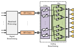
(a) Fully-connected architecture.

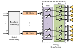
(b) Proposed sub-connected architecture.

Figure 2: Architectures for TTD-based hybrid beamforming.

Let $N_{\mathrm{RF}}$ denote the number of RF chains in the hybrid beamforming architecture, which is subject to the constraint $K\leq N_{\mathrm{RF}}\ll N$, and $N_{\mathrm{T}}$ denote the number of TTDs connected to each RF chain. Then, when the TTD-hybrid beamforming architecture is exploited, the received signal of user $k$ at subcarrier $m$ can be modelled as

$$y_{m,k}=\mathbf{h}_{m,k}^{H}\mathbf{A}\mathbf{T}_{m}\mathbf{D}_{m}\mathbf{s}_{m}+n_{m,k},$$ (6)

where $\mathbf{A}\in\mathbb{C}^{N\times N_{\mathrm{T}}N_{\mathrm{RF}}}$ and $\mathbf{T}_{m}\in\mathbb{C}^{N_{\mathrm{T}}N_{\mathrm{RF}}\times N_{\mathrm{RF}}}$ denote the frequency-independent and frequency-dependent analog beamformers realized by TTDs and PSs, respectively, $\mathbf{D}_{m}\in\mathbb{C}^{N_{\mathrm{RF}}\times K}$ denotes the baseband digital beamformer, $\mathbf{s}_{m}\in\mathbb{C}^{K\times 1}$ denotes the information symbols of the $K$ users at subcarrier $m$, satisfying $\mathbb{E}[\mathbf{s}_{m}\mathbf{s}_{m}^{H}]=\mathbf{I}_{K}$, and $n_{m,k}\sim\mathcal{CN}(0,\sigma_{m,k}^{2})$ represents the additive Gaussian white noise. In particular, for both fully-connected and sub-connected architectures, the TTD-based analog beamformer is given by

$$\mathbf{T}_{m}=\mathrm{blkdiag}\left(e^{-j2\pi f_{m}\mathbf{t}_{1}},\dots,e^{-j2\pi f_{m}\mathbf{t}_{N_{\mathrm{RF}}}}\right),$$ (7)

where $\mathbf{t}_{n}=[t_{n,1},\dots,t_{n,N_{\mathrm{T}}}]\in\mathbb{R}^{N_{\mathrm{T}}\times 1}$ denotes the time-delay vector realized the TTDs connected to the $n$-th RF chain. The time delay of each TTD needs to satisfy the maximum delay constraint, i.e., $t_{n,l}\in[0,t_{\max}],\forall n=1,...,N_{\mathrm{RF}},l=1,\dots,N_{\mathrm{T}}$. The PS-based analog beamformer $\mathbf{A}$ are of different structures for the fully-connected and sub-connected architectures, which are detailed in the following.

• Fully-Connected Architecture: In this architecture, each TTD is connected to $N/N_{\mathrm{T}}$ antennas via PSs. Therefore, the PS-based analog beamformer $\mathbf{A}$ for the fully-connected architecture is given by

  $$\mathbf{A}=[\mathbf{A}_{1},\dots,\mathbf{A}_{N_{\mathrm{RF}}}],$$ (8)

  $$\mathbf{A}_{n}=\mathrm{blkdiag}(\mathbf{a}_{n,1},...,\mathbf{a}_{n,N_{\mathrm{T}}}),$$ (9)

  where $\mathbf{A}_{n}\in\mathbb{C}^{N\times N_{\mathrm{T}}}$ and $\mathbf{a}_{n,l}\in\mathbb{C}^{\frac{N}{N_{\mathrm{T}}}\times 1}$ denote the PS-based analog beamformer connected to the $n$-th RF chain and the $l$-th TTD of this chain, respectively.

• Sub-Connected Architecture: In this architecture, each RF chain is only connected to a sub-array of $N_{\mathrm{sub}}=N/N_{\mathrm{RF}}$ antennas, and thus each TTD is connected to $N_{\mathrm{sub}}/N_{\mathrm{T}}$ antennas. As a result, the corresponding PS-based analog beamformer $\mathbf{A}$ can be expressed follows:

  $$\mathbf{A}=\mathrm{blkdiag}(\mathbf{A}_{1},\dots,\mathbf{A}_{N_{\mathrm{RF}}}),$$ (10)

  $$\mathbf{A}_{n}=\mathrm{blkdiag}(\mathbf{a}_{n,1},\dots,\mathbf{a}_{n,N_{\mathrm{T}}}),$$ (11)

  where $\mathbf{A}_{n}\in\mathbb{C}^{N_{\mathrm{sub}}\times N_{\mathrm{T}}}$ and $\mathbf{a}_{n,l}\in\mathbb{C}^{\frac{N_{\mathrm{sub}}}{N_{\mathrm{T}}}\times 1}$ denote the PS-based analog beamformer for the sub-array connected to the $n$-th RF chain and the $l$-th TTD of this chain, respectively.

Moreover, due to the inherent limitations of PSs, which can only adjust the phase of the signals, the analog beamformer based on PSs must satisfy the unit-modulus constraint. In other words, for non-zero entries, the PS-based analog beamformer should satisfy $|[\mathbf{A}]_{i,j}|=1$.

Remark 1.

(Advantages of the proposed sub-connected architecture) Compared to the fully-connected architecture, the advantages of the sub-connected architecture are summarized as follows. Firstly, it significantly reduces the required number of PSs from $NN_{\mathrm{RF}}$ PSs in the fully-connected architecture to just $N$ PSs in the sub-connected architecture. Secondly, within the sub-connected architecture, the TTDs connected to each RF chain only need to mitigate the near-field beam split effect of individual sub-arrays. It is worth noting that this effect is relatively less significant compared to the effect on the entire array. Consequently, only a few TTDs are required for each RF chain. Based on the aforementioned analysis, the sub-connected architecture achieves high energy efficiency by the reduced number of both PSs and TTDs.

II-C Problem Formulation

We aim to maximize the spectral efficiency of the considered near-field wideband communication system by optimizing the analog and digital beamformers of the TTD-based hybrid beamforming architecture. According to (6), the achievable communication rate of user $k$ at subcarrier $m$ is given by

$$R_{m,k}=\log_{2}\left(1+\frac{|\mathbf{h}_{m,k}^{H}\mathbf{A}\mathbf{T}_{m}\mathbf{d}_{m,k}|^{2}}{\sum_{i\in\mathcal{K},i\neq k}|\mathbf{h}_{m,k}^{H}\mathbf{A}\mathbf{T}_{m}\mathbf{d}_{m,i}|^{2}+\sigma_{m,k}^{2}}\right),$$ (12)

where $\mathbf{d}_{m,k}\in\mathbb{C}^{N_{\mathrm{RF}}\times 1}$ represents the $k$-th column of $\mathbf{D}_{m}$ and also the digital beamformer of user $k$ at subcarrier $m$. Therefore, the spectral efficiency maximization problem can be formulated as follows:

$$\max_{\mathbf{A},\mathbf{T}_{m},\mathbf{D}_{m}}\quad \sum_{m\in\mathcal{M}}\sum_{k\in\mathcal{K}}R_{m,k}(\mathbf{A},\mathbf{T}_{m},\mathbf{D}_{m})$$ (13a)

$$\mathrm{s.t.}\quad \|\mathbf{A}\mathbf{T}_{m}\mathbf{D}_{m}\|_{F}^{2}\leq P_{t},\forall m,$$ (13b)

$$\mathbf{A}\in\mathcal{A},\mathbf{T}_{m}\in\mathcal{T}_{m},\forall m.$$ (13c)

Specifically, constraint (13b) is the maximum transmit power constraint, where $P_{t}$ denotes the maximum transmit power available for each subcarrier. $\mathcal{A}\in\{\mathcal{A}_{F},\mathcal{A}_{P}\}$ is the feasible set of the PS-based analog beamformers imposed by the unit-modulus constraint for fully-connected or sub-connected architectures. $\mathcal{T}_{m}$ is the feasible set of the TTD-based analog beamformers imposed by the formula (7) and the maximum time delay constraint. Problem (13) is challenging to solve due to the following reasons.

• Firstly, the analog and digital beamformers are highly coupled in the non-convex sum-of-logarithms objective function and the maximum transmit power constraint.

• Secondly, the entries of the PS-based analog beamformer $\mathbf{A}$ are subject to the non-convex unit-modulus constraints.

• Thirdly, the TTD-based analog beamformers $\mathbf{T}_{m},\forall m,$ exhibit a complex exponential form. Furthermore, they are coupled across different subcarriers due to their implementation using a shared set of time delays. The fixed interval constraints on these time delays, i.e., $t_{n,l}\in[0,t_{\max}],\forall n,l$, pose additional challenges in achieving joint optimization of all time delays.

To the best of the authors’ knowledge, there are no general solutions to problem (13) in the presence of the above challenges. Therefore, in the following, we propose three efficient approaches to address this problem, namely the FDA approach, the penalty-based FDA approach, and the low-complexity HTS approach.

III Fully-digital Approximation Approach

In this section, we develop an FDA approach to solve problem (13). The main idea of the FDA approach is to optimize the hybrid beamformer sufficiently “close” to the optimal unconstrained fully-digital beamformer. This idea has been widely exploited for optimizing the conventional hybrid beamformers [21, 11].

III-A Problem Reformulation

In this subsection, we reformulate problem (13) into an FDA problem. The first step is to obtain the optimal unconstrained fully-digital beamformer by solving the following problem:

$$\max_{\mathbf{P}_{m}}\quad \sum_{m\in\mathcal{M}}\sum_{k\in\mathcal{K}}\tilde{R}_{m,k}(\mathbf{P}_{m})$$ (14a)

$$\mathrm{s.t.}\quad \|\mathbf{P}_{m}\|_{F}^{2}\leq P_{t},\forall m,$$ (14b)

where $\mathbf{P}_{m}=[\mathbf{p}_{m,1},\dots,\mathbf{p}_{m,K}]\in\mathbb{C}^{N\times K}$ is the unconstrained fully-digital beamformer for subcarrier $m$ and $\tilde{R}_{m,k}$ is the corresponding achievable rate given by

$$\tilde{R}_{m,k}=\log_{2}\left(1+\frac{|\mathbf{h}_{m,k}^{H}\mathbf{p}_{m,k}|^{2}}{\sum_{i\in\mathcal{K},i\neq k}|\mathbf{h}_{m,k}^{H}\mathbf{p}_{m,i}|^{2}+\sigma_{m,k}^{2}}\right).$$ (15)

This optimization problem has been well investigated in the literature. Existing methods, such as fractional programming (FP) [22], successive convex approximation (SCA) [23], and weighted minimum mean-square error (WMMSE) [24] methods, have proven to be effective in obtaining a stationary point for this problem. Thus, we omit the details for solving problem (14) here. Let $\mathbf{P}_{m}^{\mathrm{opt}}$ denote a stationary-point solution to problem (14) obtained by the aforementioned methods. Then, the analog and digital beamformers of the TTD-based hybrid beamforming architecture can be optimized to approximate $\mathbf{P}_{m}^{\mathrm{opt}}$, resulting in the following problem:

$$\min_{\mathbf{A},\mathbf{T}_{m},\mathbf{D}_{m}}\quad \sum_{m\in\mathcal{M}}\|\mathbf{P}_{m}^{\mathrm{opt}}-\mathbf{A}\mathbf{T}_{m}\mathbf{D}_{m}\|_{F}^{2}$$ (16a)

$$\mathrm{s.t.}\quad \mathbf{A}\in\mathcal{A},\mathbf{T}_{m}\in\mathcal{T}_{m},\forall m.$$ (16b)

Problem (16) is to minimize the distance between the hybrid beamformers and the optimal fully digital beamformer, which will also approximately maximize the spectral efficiency. It is worth noting that the maximum transmit power constraint is omitted in problem (16). After obtaining the optimal solution of $\mathbf{A}$, $\mathbf{T}_{m}$, and $\mathbf{D}_{m}$, the digital beamformer $\mathbf{D}_{m}$ can be normalized by a factor $\sqrt{P_{t}}/\|\mathbf{A}\mathbf{T}_{m}\mathbf{D}_{m}\|_{F}$ to satisfy the maximum transmit power constraint. According to [11, Lemma 1], the normalization operation only leads to a negligible performance loss. In the following, we solve problem (16) for fully-connected and sub-connected architectures, respectively.

III-B Solution for Fully-Connected Architectures

For fully-connected architectures, the analog beamformer matrix $\mathbf{A}\mathbf{T}_{m}$ is a full matrix, resulting in the coupling between time delay of different TTDs. To address this issue, we introduce the auxiliary variable $\mathbf{V}_{m}\in\mathbb{C}^{N\times N_{RF}}$. Each element of $\mathbf{V}_{m}$ is subject to the unit-modulus constraint, i.e., $|[\mathbf{V}_{m}]_{i,j}|=1$. Therefore, problem (16) for fully-connected architectures can be approximated by

$$\min_{\scriptstyle\mathbf{V}_{m},\mathbf{A},\atop\scriptstyle\mathbf{T}_{m},\mathbf{D}_{m}} \sum_{m\in\mathcal{M}}\|\mathbf{P}_{m}^{\mathrm{opt}}-\mathbf{V}_{m}\mathbf{D}_{m}\|_{F}^{2}+\varrho\sum_{m\in\mathcal{M}}\|\mathbf{V}_{m}-\mathbf{A}\mathbf{T}_{m}\|_{F}^{2}$$ (17a)

$$\mathrm{s.t.}\quad |[\mathbf{V}_{m}]_{i,j}|=1,\forall i,j,$$ (17b)

$$\mathbf{A}\in\mathcal{A},\mathbf{T}_{m}\in\mathcal{T}_{m},\forall m.$$ (17c)

where $\varrho>0$ is a regularization factor that determines the priority of the two terms in the objective function. To solve this new optimization problem, we propose to exploit the BCD, where the variable blocks $\mathbf{A}$, $\mathbf{T}_{m}$, $\mathbf{V}_{m}$, and $\mathbf{D}_{m}$ are optimized in an alternating manner.

III-B1 Optimization of PS-based Analog Beamformers

The optimization problem for the matrix $\mathbf{A}$ is given by

$$\min_{\mathbf{A}}\quad \sum_{m\in\mathcal{M}}\left\|\mathbf{V}_{m}-\mathbf{A}\mathbf{T}_{m}\right\|_{F}^{2}$$ (18a)

$$\mathrm{s.t.}\quad \mathbf{A}\in\mathcal{A}_{F}.$$ (18b)

By defining $\mathbf{v}_{m,n,l}=[\mathbf{V}_{m}]_{(l-1)\frac{N}{N_{\mathrm{T}}}+1:l\frac{N}{N_{\mathrm{T}}},n}$, the objective function can be recast as

$$\eqref{obj_1}=\sum_{n=1}^{N_{\mathrm{RF}}}\sum_{l=1}^{N_{\mathrm{T}}}\sum_{m\in\mathcal{M}}\|\mathbf{v}_{m,n,l}-\mathbf{a}_{n,l}e^{-j2\pi f_{m}t_{n,l}}\|^{2}.$$ (19)

It is evident that the objective function is separable. Consequently, each vector $\mathbf{f}_{n,l}$ can be optimized independently, leading to the following individual optimization problem:

$$\min_{\mathbf{a}_{n,l}}\quad \sum_{m\in\mathcal{M}}\left\|\mathbf{v}_{m,n,l}-\mathbf{a}_{n,l}e^{-j2\pi f_{m}t_{n,l}}\right\|^{2}$$ (20a)

$$\mathrm{s.t.}\quad |[\mathbf{a}_{n,l}]_{i}|=1,\forall i.$$ (20b)

To solve this optimization problem, we further simplify its objective function as follows:

$$\eqref{obj_2}= \sum_{m\in\mathcal{M}}-2\mathrm{Re}\left\{\mathbf{v}_{m,n,l}^{H}\mathbf{a}_{n,l}e^{-j2\pi f_{m}t_{n,l}}\right\}$$

$$+\sum_{m\in\mathcal{M}}\!\!\mathbf{a}_{n,l}^{H}\mathbf{a}_{n,l}+\mathbf{v}_{m,n,l}^{H}\mathbf{v}_{m,n,l}.$$ (21)

By exploiting the unit-modulus constraints of $\mathbf{a}_{n,l}$ and $\mathbf{v}_{m,n,l}$, we have $\mathbf{a}_{n,l}^{H}\mathbf{a}_{n,l}=\mathbf{v}_{m,n,l}^{H}\mathbf{v}_{m,n,l}=MN/N_{\mathrm{T}}$. Therefore, problem (20) is equivalent to minimizing the first term of the above expression subject to the unit-modulus constraint, resulting in the following optimal solution:

$$\mathbf{a}_{n,l}=e^{j\angle\tilde{\mathbf{v}}_{n,l}},$$ (22)

where $\tilde{\mathbf{v}}_{n,l}=\sum_{m\in\mathcal{M}}\mathbf{v}_{m,n,l}e^{j2\pi f_{m}t_{n,l}}$.

III-B2 Optimization of TTD-based Analog Beamformers

Next, we optimize the TTD-based analog beamformer $\mathbf{T}_{m},\forall m,$ by fixing the other optimization variables. The resulting optimization is given by

$$\min_{\mathbf{T}_{m}}\quad \sum_{m\in\mathcal{M}}\|\mathbf{V}_{m}-\mathbf{A}\mathbf{T}_{m}\|_{F}^{2}$$ (23a)

$$\mathrm{s.t.}\quad \mathbf{T}_{m}\in\mathcal{T}_{m},\forall m.$$ (23b)

According to the result in (19) and (III-B1), the above optimization problem is also a separable problem with respect to each time delay $t_{n,l},\forall n,l$, leading to the following independent optimization problem for each $t_{n,l}$:

$$\min_{t_{n,l}}\quad \sum_{m\in\mathcal{M}}\mathrm{Re}\left\{\mathbf{v}_{m,n,l}^{H}\mathbf{a}_{n,l}e^{-j2\pi f_{m}t_{n,l}}\right\}$$ (24a)

$$\mathrm{s.t.}\quad t_{n,l}\in[0,t_{\max}].$$ (24b)

The above problem can be categorized as a single-variable optimization problem within a fixed interval, which can be handled using standard techniques, such as linear search.

III-B3 Optimization of Auxiliary Variables

The optimization problem with respect to the auxiliary variable $\mathbf{V}_{m},\forall m,$ by fixing the other optimization variables is given by

$$\min_{\mathbf{V}_{m}}\quad \|\mathbf{P}_{m}^{\mathrm{opt}}-\mathbf{V}_{m}\mathbf{D}_{m}\|_{F}^{2}+\varrho\|\mathbf{V}_{m}-\mathbf{A}\mathbf{T}_{m}\|_{F}^{2}$$ (25a)

$$\mathrm{s.t.}\quad |[\mathbf{V}_{m}]_{i,j}|=1,\forall i,j.$$ (25b)

To address the element-wise unit-modulus constraint, we optimize $\mathbf{V}_{m}$ in a coordinate descent manner. Specifically, each entry of $\mathbf{V}_{m}$ is optimized in one step by fixing the other entries. Firstly, after some algebraic manipulations, the optimization problem (25) can be recast as

$$\min_{\mathbf{V}_{m}}\quad \mathrm{tr}\left(\mathbf{V}_{m}^{H}\mathbf{V}_{m}\mathbf{\Phi}_{m}\right)-\mathrm{Re}\left\{\mathrm{tr}\left(\mathbf{V}_{m}^{H}\mathbf{\Psi}_{m}\right)\right\}$$ (26a)

$$\mathrm{s.t.}\quad |[\mathbf{V}_{m}]_{i,j}|=1,\forall i,j,$$ (26b)

where $\mathbf{\Phi}_{m}=\mathbf{D}_{m}\mathbf{D}_{m}^{H}+\varrho\mathbf{I}_{N_{\mathrm{RF}}}$ and $\mathbf{\Psi}_{m}=\mathbf{P}_{m}^{\mathrm{opt}}\mathbf{D}_{m}^{H}+\varrho\mathbf{A}\mathbf{T}_{m}$. Then, the optimization problem for the $(i,j)$-th entry of $\mathbf{V}_{m}$ by fixing the other entries is given by

$$\min_{[\mathbf{V}_{m}]_{i,j}}\quad c_{m,i,j}|[\mathbf{V}_{m}]_{i,j}|^{2}-2\mathrm{Re}\left\{d_{m,i,j}^{*}[\mathbf{V}_{m}]_{i,j}\right\}$$ (27a)

$$\mathrm{s.t.}\quad |[\mathbf{V}_{m}]_{i,j}|=1,$$ (27b)

where $c_{m,i,j}=[\mathbf{\Phi}_{m}]_{j,j}$ and $d_{m,i,j}=[\mathbf{\Phi}_{m}]_{j,j}[\mathbf{V}_{m}]_{i,j}-[\mathbf{V}_{m}\mathbf{\Phi}_{m}]_{i,j}+[\mathbf{\Psi}_{m}]_{i,j}$. Due to the unit-modulus constraint, the first term in the objective function of problem (27) is a constant, i.e., $c_{m,i,j}|[\mathbf{V}_{m}]_{i,j}|^{2}=c_{m,i,j}$. As a result, problem (27) is equivalent to maximizing the $\mathrm{Re}\left\{d_{m,i,j}^{*}[\mathbf{V}_{m}]_{i,j}\right\}$ subject to the unit-modulus constraint, which has the following optimal solution:

$$[\mathbf{V}_{m}]_{i,j}=e^{j\angle d_{m,i,j}}.$$ (28)

The coordinate descent algorithm for solving problem (25) is summarized in Algorithm 1.

Algorithm 1 Coordinate descent algorithm for solving (25).

1:  initialize $\mathbf{V}_{m},\forall m$.

2:  repeat

3:     for  $i\in\{1,\dots,N\},j\in\{1,\dots,N_{\mathrm{RF}}\}$  do

4:        update $[\mathbf{V}_{m}]_{i,j}$ according to (28)

5:     end for

6:  until some termination criterion is met.

III-B4 Optimization of Digital Beamformers

The optimization problem for the digital beamformer $\mathbf{D}_{m}$ is given by

$$\min_{\mathbf{D}_{m}}\quad\|\mathbf{P}_{m}^{\mathrm{opt}}-\mathbf{V}_{m}\mathbf{D}_{m}\|_{F}^{2}.$$ (29)

This problem is a well-known least square problem, yielding the following optimal solution:

$$\mathbf{D}_{m}=\mathbf{V}_{m}^{\dagger}\mathbf{P}_{m}^{\mathrm{opt}}.$$ (30)

The FDA approach based on BCD for fully-connected architectures is summarized in Algorithm 2. Since the objective value is non-increasing in each step of BCD and is bounded from below, the convergence of Algorithm 2 is guaranteed. Furthermore, Algorithm 2 is computationally efficient, as the optimization variables in each step are updated by either the closed-form solution or the low-complexity linear search. It can be shown that the complexity of updating $\mathbf{A}$ is $\mathcal{O}(MN)$, that of updating $\mathbf{T}_{m},\forall m,$ is $\mathcal{O}(MN^{2}N_{\mathrm{RF}}Q/N_{\mathrm{T}})$ where $Q$ is the number of steps in linear search, that of updating $\mathbf{V}_{m},\forall m,$ is $\mathcal{O}(\sum_{m}I_{m}(N_{\mathrm{RF}}^{2}K+2NN_{\mathrm{RF}}K+NN_{\mathrm{RF}}^{2}N_{\mathrm{T}}))$, where $I_{m}$ is the number of iterations, and that of updating $\mathbf{D}_{m},\forall m,$ is $\mathcal{O}(M(2NN_{\mathrm{RF}}^{2}+N_{\mathrm{RF}}^{3}+NN_{\mathrm{RF}}K))$.

III-C Solution for Sub-Connected Architectures

For the sub-connected architecture, the matrix $\mathbf{A}\mathbf{T}_{m}$ is not a full matrix. By exploiting this spectral structure of the matrix $\mathbf{A}\mathbf{T}_{m}$, problem (16) can be effectively solved by BCD without introducing the auxiliary variables. Similarly, the optimization variables are divided into three blocks, namely $\mathbf{A}$, $\mathbf{T}_{m}$, and $\mathbf{D}_{m}$.

III-C1 Optimization of PS-based Analog Beamformers

Recall that the PS-based analog beamformer in the sub-connected architecture is given by

$$\mathbf{A}=\mathrm{blkdiag}(\mathbf{A}_{1},\dots,\mathbf{A}_{N_{\mathrm{RF}}}),$$ (31)

$$\mathbf{A}_{n}=\mathrm{blkdiag}(\mathbf{a}_{n,1},\dots,\mathbf{a}_{n,N_{\mathrm{T}}}),$$ (32)

Thus, by defining $\tilde{\mathbf{P}}_{m,n}=[\mathbf{P}_{m}^{\mathrm{opt}}]_{(n-1)N_{\mathrm{sub}}+1:nN_{\mathrm{sub}},:}$, $\tilde{\mathbf{d}}_{m,n}=[\mathbf{D}_{m}^{H}]_{:,n}$, the objective function of problem (16) can be simplified as follows:

$$\eqref{obj_3}=\sum_{n=1}^{N_{\mathrm{RF}}}\sum_{m\in\mathcal{M}}\left\|\tilde{\mathbf{P}}_{m,n}-\mathbf{A}_{n}e^{-j2\pi f_{m}\mathbf{t}_{n}}\tilde{\mathbf{d}}_{m,n}^{H}\right\|_{F}^{2}$$

$$=-\sum_{n=1}^{N_{\mathrm{RF}}}\sum_{m\in\mathcal{M}}2\mathrm{Re}\left\{\tilde{\mathbf{d}}_{m,n}^{H}\tilde{\mathbf{P}}_{m,n}^{H}\mathbf{A}_{n}e^{-j2\pi f_{m}\mathbf{t}_{n}}\right\}$$

$$+\sum_{n=1}^{N_{\mathrm{RF}}}\sum_{m\in\mathcal{M}}\tilde{\mathbf{d}}_{m,n}^{H}\tilde{\mathbf{d}}_{m,n}e^{j2\pi f_{m}\mathbf{t}_{n}^{T}}\mathbf{A}_{n}^{H}\mathbf{A}_{n}e^{-j2\pi f_{m}\mathbf{t}_{n}}+C,$$ (33)

where $C$ is a constant independent of $\mathbf{A}$. It can also be readily proved that $e^{j2\pi f_{m}\mathbf{t}_{n}^{T}}\mathbf{A}_{n}^{H}\mathbf{A}_{n}e^{-j2\pi f_{m}\mathbf{t}_{n}}=N_{\mathrm{sub}}$, which renders the second term in the above formula is also independent of $\mathbf{A}$. Then, by defining $\boldsymbol{\upsilon}_{m,n,l}=[\tilde{\mathbf{P}}_{m,n}\tilde{\mathbf{d}}_{m,n}]_{(l-1)\frac{N_{\mathrm{sub}}}{N_{\mathrm{T}}}+1:l\frac{N_{\mathrm{sub}}}{N_{\mathrm{T}}}}$, objective function with respect to $\mathbf{A}$ can be further simplified as follows:

$$\eqref{obj_3}=-\sum_{n=1}^{N_{\mathrm{RF}}}\sum_{l=1}^{N_{\mathrm{T}}}\sum_{m\in\mathcal{M}}2\mathrm{Re}\left\{\boldsymbol{\upsilon}_{m,n,l}^{H}\mathbf{a}_{n,l}e^{-j2\pi f_{m}t_{n,l}}\right\}+\tilde{C},$$ (34)

where $\tilde{C}$ collects all constant terms. Thus, each vector $\mathbf{a}_{n,l}$ can be designed individually by solving the following problem:

$$\max_{\mathbf{a}_{n,l}}\quad \mathrm{Re}\left\{\boldsymbol{\upsilon}_{m,n,l}^{H}\mathbf{a}_{n,l}e^{-j2\pi f_{m}t_{n,l}}\right\}$$ (35a)

$$\mathrm{s.t.}\quad |[\mathbf{a}_{n,l}]_{i}|=1,\forall i.$$ (35b)

By defining $\tilde{\boldsymbol{\upsilon}}_{n,l}=\sum_{m\in\mathcal{M}}\boldsymbol{\upsilon}_{m,n,l}e^{j2\pi f_{m}t_{n,l}}$, the optimal solution to this problem is given by

$$\mathbf{a}_{n,l}=e^{j\angle\tilde{\boldsymbol{\upsilon}}_{m,n,l}}.$$ (36)

We note that for the sub-connected architecture, the analog beamformer for each RF chain is not coupled with each other, which simplifies the optimization process.

Algorithm 2 Proposed FDA Approach for Fully-Connected Architectures.

1:  initialize $\mathbf{A}$, $\mathbf{T}_{m}$, $\mathbf{D}_{m}$, $\mathbf{V}_{m},\forall m$.

2:  repeat

3:     update $\mathbf{A}$ according to (22).

4:     update $\mathbf{T}_{m}$ by solving (24) via linear search.

5:     update $\mathbf{V}_{m}$ via Algorithm 1

6:     update $\mathbf{D}_{m}$ according to (30).

7:  until some termination criterion is met.

8:  normalized the obtained digital beamformers as $\mathbf{D}_{m}=\frac{\sqrt{P_{t}}}{\|\mathbf{A}\mathbf{T}_{m},\mathbf{D}_{m}\|_{F}}\mathbf{D}_{m}$.

III-C2 Optimization of TTD-based Analog Beamformers

According to the results in (34), the TTD-based analog beamformer $\mathbf{T}_{m}$ can be optimized by optimizing each time delay $t_{n,l}$ independently, resulting in the following optimization problem:

$$\max_{t_{n,l}}\quad \sum_{m\in\mathcal{M}}2\mathrm{Re}\{\boldsymbol{\upsilon}_{m,n,l}^{H}\mathbf{a}_{n,l}e^{-j2\pi f_{m}t_{n,l}}\}$$ (37a)

$$\mathrm{s.t.}\quad t_{n,l}\in[0,t_{\max}].$$ (37b)

This problem exhibits a similar structure to problem (24), which can also be solved by the linear search.

III-C3 Optimization of Digital Beamformers

The subproblem with respect to the digital beamformer is given by

$$\min_{\mathbf{D}_{m}}\quad\left\|\mathbf{P}_{m}^{\mathrm{opt}}-\mathbf{A}\mathbf{T}_{m}\mathbf{D}_{m}\right\|_{F}^{2},\vspace{-0.2cm}$$ (38)

which has the following optimal least-square solution:

$$\mathbf{D}_{m}=(\mathbf{A}\mathbf{T}_{m})^{\dagger}\mathbf{P}_{m}^{\mathrm{opt}}.$$ (39)

The FDA approach based on BCD for sub-connected architectures is summarized in Algorithm 3. In each step of Algorithm 3, the complexities for updating $\mathbf{A}$, $\mathbf{T}_{m}$, and $\mathbf{D}_{m}$, are given by $\mathcal{O}(M(N^{2}K^{2}+N))$, $\mathcal{O}(MN^{2}Q/(N_{\mathrm{RF}}N_{\mathrm{T}}))$, and $\mathcal{O}(M(2NN_{\mathrm{RF}}^{2}+N_{\mathrm{RF}}^{3}+NN_{\mathrm{RF}}K+NN_{\mathrm{RF}}^{3}N_{\mathrm{T}}^{2}))$, respectively.

Algorithm 3 Proposed FDA Approach for Sub-Connected Architectures.

1:  initialize $\mathbf{A}$, $\mathbf{T}_{m}$, $\mathbf{D}_{m},\forall m$.

2:  repeat

3:     update $\mathbf{A}$ according to (36).

4:     update $\mathbf{T}_{m}$ by solving (37) via linear search.

5:     update $\mathbf{D}_{m}$ according to (39).

6:  until some termination criterion is met.

7:  normalized the obtained digital beamformers as $\mathbf{D}_{m}=\frac{\sqrt{P_{t}}}{\|\mathbf{A}\mathbf{T}_{m},\mathbf{D}_{m}\|_{F}}\mathbf{D}_{m}$.

IV Penalty-based FDA Approach

Although the FDA approach can obtain a solution for the hybrid beamformer that closely approximates the unconstrained fully-digital beamformer, it does not directly address the problem of maximizing spectral efficiency and does not incorporate channel state information (CSI) into the optimization process. Therefore, it is difficult to guarantee the optimality of the obtained solution. In certain scenarios, the FDA approach may lead to significant performance degradation, because approximating the unconstrained fully-digital beamformer is not always approximately maximizing the spectral efficiency. As a remedy, we further propose a penalty-based FDA approach, where the hybrid beamformer is optimized to directly maximize spectral efficiency.

The key idea of the penalty-based FDA approach is to jointly optimize the unconstrained fully-digital beamformer $\mathbf{P}_{m}$ and the hybrid beamformers $\{\mathbf{A},\mathbf{T}_{m},\mathbf{D}_{m}\}$ with the aid of the penalty method. Firstly, we transform the original spectral efficiency maximizing problem (13) into the following equivalent optimization problem:

$$\max_{\scriptstyle\mathbf{P}_{m},\mathbf{A},\atop\scriptstyle\mathbf{T}_{m},\mathbf{D}_{m}}\quad \sum_{m\in\mathcal{M}}\sum_{k\in\mathcal{K}}\tilde{R}_{m,k}(\mathbf{P}_{m})$$ (40a)

$$\mathrm{s.t.}\quad \mathbf{P}_{m}=\mathbf{A}\mathbf{T}_{m}\mathbf{D}_{m},$$ (40b)

$$\|\mathbf{P}_{m}\|_{F}^{2}\leq P_{t},\forall m,$$ (40c)

$$\mathbf{A}\in\mathcal{A},\mathbf{T}_{m}\in\mathcal{T}_{m},\forall m,$$ (40d)

where $\tilde{R}_{m,k}(\mathbf{P}_{m})$ is given in (15). Then, the penalty method can be used to move the equality constraint (40b) as a penalty term to the objective function [25]. The resulting optimization problem is given by

$$\max_{\scriptstyle\mathbf{P}_{m},\mathbf{A},\atop\scriptstyle\mathbf{T}_{m},\mathbf{D}_{m}} \sum_{m\in\mathcal{M}}\sum_{k\in\mathcal{K}}\tilde{R}_{m,k}(\mathbf{P}_{m})-\frac{1}{\rho}\sum_{m\in\mathcal{M}}\left\|\mathbf{P}_{m}-\mathbf{A}\mathbf{T}_{m}\mathbf{D}_{m}\right\|_{F}^{2}$$ (41a)

$$\mathrm{s.t.}\quad \eqref{penalty_cons_1},\eqref{penalty_cons_2},$$ (41b)

where $\rho>0$ is a penalty factor. In particular, when $\rho\rightarrow 0$, the penalty term can be exactly zero, which yields a solution to problem (40). However, to ensure optimal performance, the penalty factor is typically initialized with a large value, ensuring that the term $\sum_{m\in\mathcal{M}}\sum_{k\in\mathcal{K}}\tilde{R}_{m,k}(\mathbf{P}_{m})$ is sufficiently maximized. Subsequently, the penalty factor is gradually decreased to guarantee the penalty term approaches zero, i.e., the equality constraint is achieved.

Algorithm 4 Proposed Penalty-based FDA Approach.

1:  initialize $\rho>0$, $\mathbf{P}_{m}$, $\mathbf{D}_{m}$, $\mathbf{V}_{m}$, $\mathbf{A}$, $\mathbf{T}_{m}$.

2:  repeat

3:     repeat

4:        update $\mathbf{P}_{m}$ based on existing methods [22, 23, 24].

5:        update $\mathbf{A}$, $\mathbf{T}_{m}$, and $\mathbf{D}_{m}$ following steps 3-6 in Algorithm 2 for fully-connected architectures and steps 3-5 in Algorithm 3 for sub-connected architectures.

6:     until some termination criterion is met.

7:     set $\rho=\epsilon\rho$.

8:  until the value of the penalty term falls below a predefined threshold.

When the fixed penalty factor, problem (41) can be effectively solved by BCD. In particular, for block $\mathbf{P}_{m}$, its subproblem can also be solved by the existing FD, SCA, and WMMSE methods, as the penalty term is convex with respect to $\mathbf{P}_{m}$. For the blocks $\mathbf{A}$, $\mathbf{T}_{m}$, and $\mathbf{D}_{m}$, their subproblems are only related to the penalty term, which is equivalent to the problem (16). Thus, they can be optimized following steps 3-6 in Algorithm 2 for fully-connected architectures and steps 3-5 in Algorithm 3 for sub-connected architectures. The penalty-based FDA approach is summarized in Algorithm 4, where $0<\epsilon<1$ is a reduction factor of the penalty factor. According to the results in [25], the penalty-based FDA approach can converge to a stationary point of problem (13). However, the complexity of the penalty-based FDA approach can be very high, as it involves jointly optimizing the high-dimensional fully-digital beamformer and the hybrid beamformers in a double-loop structure. The detailed complexity can be easily obtained based on the complexity of Algorithms 2 and 3 as well as the complexity of the methods in [22, 23, 24].

V Low-complexity Heuristic Two-stage Approach

Although the FDA approach directly optimized the hybrid beamformer and can obtain a stationary point with the aid of the penalty method, it has the following drawbacks that hinder its practical implementation.

• Firstly, the FDA approach requires optimizing the equivalent fully-digital beamformers and the analog beamformers. In near-field communications with ELAAs, the dimension of these beamformers is typically quite large, which leads to high computational complexity for solving this optimization problem.

• Secondly, the FDA approach requires full knowledge of the CSI. Similarly, due to the large number of antenna elements in near-field communications, the complexity of the channel estimation can be extremely high.

To address these issues, in this section, we propose an HTS approach, where the analog and digital beamformers are designed in two separate stages. This approach not only significantly reduces the complexity of optimization, but also simplifies channel estimation with the aid of fast near-field beam training [26]. In particular, the communication protocol including the proposed HTS approach and beam training is illustrated in Fig. 3, which will be detailed in the following.

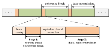
Figure 3: Communication protocol including the proposed HTS approach and beam training.

V-A Heuristic Analog Beamformer Design

Before designing the analog beamformers, the near-field beam training [26] is carried out, where the location of each user $k$, i.e., $\theta_{k}$ and $\nu_{k}$, can be obtained. During the near-field beam training, the near-field beam split effect can be avoided by exploiting only a small portion of the bandwidth. Therefore, we have obtained part of the CSI of the LoS channels. It is worth noting that due to the high carrier frequencies in near-field communications, the NLoS path loss can be much higher that the LoS path loss. Therefore, for designing the analog beamformers, we only focus on the LoS channels, resulting in the following received signal of user $k$ at subcarrier $m$:

$$y_{m,k}\approx\beta_{m,k}\mathbf{b}_{N}^{T}(f_{m},\theta_{k},\nu_{k})\mathbf{A}\mathbf{T}_{m}\mathbf{D}_{m}\mathbf{s}_{m}+n_{m,k}.$$ (42)

Based on the above signal model and the knowledge of $\theta_{k}$ and $\nu_{k}$ obtained by beam training, we propose a heuristic closed-form design of the analog beamformer for the fully-connected architecture, which can be easily extended to the sub-connected architectures. Therefore, in the following, we focus on the fully-connected architecture.

In the HTS approach, we design the analog beamformer connected to each RF chain to maximize the array gain at a specific user. Specifically, analog beamformers connected to the first $K$ out of $N_{\mathrm{RF}}$ RF chains are designed to maximize the array gain of each user individually, while the remaining analog beamformers are designed to randomly focus on a particular user based on the law of least repetition to ensure fairness. We first design the analog beamformers of the first $K$ RF chains. Define the overall analog beamformer as $\mathbf{V}_{m}=\mathbf{A}\mathbf{T}_{m}$. Then, the $k$-th column of $\mathbf{V}_{m}$ denotes the overall analog beamformer for the $k$-th RF chain at the subcarrier $m$, which can be expressed as

$$\mathbf{v}_{m,k}=\begin{bmatrix}\mathbf{a}_{k,1}e^{-j2\pi f_{m}t_{k,1}}\\[-3.99994pt] \vdots\\ \mathbf{a}_{k,N_{\mathrm{T}}}e^{-j2\pi f_{m}t_{k,N_{\mathrm{T}}}}\end{bmatrix}.$$ (43)

Ideally, given the location information $\theta_{k}$ and $\nu_{k}$ of user $k$, the optimal analog beamformer $\mathbf{w}_{m,k}$ that maximizes the array gain at user $k$ at subcarrier $m$ is given by

$$\mathbf{w}_{m,k}^{\mathrm{opt}}= \arg\max_{\mathbf{w}_{m,k}}\big{|}\mathbf{b}_{N}^{T}(f_{m},\theta_{k},\nu_{k})\mathbf{w}_{m,k}\big{|}$$

$$= \mathbf{b}_{N}^{*}(f_{m},\theta_{k},\nu_{k})e^{j\psi_{m,k}},\forall m,$$ (44)

where $\psi_{m,k}$ is an arbitrary phase. Unfortunately, due to the hardware limitation imposed on $\mathbf{v}_{m,k}$, it is generally impossible to find $\mathbf{a}_{k,l}$ and $t_{k,l},\forall l,$ such that $\mathbf{v}_{m,k}=\mathbf{w}_{m,k}^{\mathrm{opt}},\forall m$. As a remedy, in the following, we propose a high-quality piecewise-near-field approximation of the near-field array response vector. Then, based on this approximation, a nearly-optimal closed-form solution of $\mathbf{v}_{m,k}$ that maximizes the array gain at the location $(\theta_{k},\nu_{k})$ at all subcarriers can be obtained.

It can be observed that $\mathbf{v}_{m,k}$ can be decomposed into $N_{\mathrm{T}}$ sub-vectors, i.e., $\mathbf{a}_{k,l}e^{-j2\pi f_{m}t_{k,l}}\in\mathbb{C}^{\tilde{N}\times 1}$ with $\tilde{N}=N/N_{\mathrm{T}}$, which denotes the analog beamformer for the $l$-the sub-array connected to the $l$-th TTD. Based on this observation, we also divide the near-field array response vector into $N_{\mathrm{T}}$ sub-vectors as follows:

$$\mathbf{b}_{N}(f_{m},\theta_{k},\nu_{k})=\begin{bmatrix}\mathbf{q}_{1}(f_{m},\theta_{k},\nu_{k})\\[-3.99994pt] \vdots\\[-3.99994pt] \mathbf{q}_{N_{\mathrm{T}}}(f_{m},\theta_{k},\nu_{k})\end{bmatrix},$$ (45)

where $\mathbf{q}_{l}(f_{m},\theta_{k},\nu_{k})=[\mathbf{a}(f_{m},\theta_{k},\nu_{k})]_{(l-1)N_{\mathrm{T}}-1:lN_{\mathrm{T}}}\in\mathbb{C}^{\tilde{N}\times 1}$ denotes the piecewise-near-field array response vector for the $l$-th sub-array. According to the geometric relationship illustrated in Fig. 4, the coordinate of the center of the $l$-th sub-array is given by $\bar{\mathbf{s}}_{l}=[\xi_{l}d,0]$, where $\xi_{l}=(l-\frac{N_{\mathrm{T}}-1}{2})\tilde{N},\forall l=0,\dots,N_{\mathrm{T}}-1$. Let $\bar{\theta}_{k,l}$ and $\bar{\nu}_{k,l}$ denote the angle and distance of the user $k$ with respect to the center of the $l$-th sub-array, respectively, which can be calculated as follows:

$$\bar{\theta}_{k,l}= \arccos\left(\frac{\nu_{k}\cos\theta_{k}-\xi_{l}d}{\bar{\nu}_{k,l}}\right),$$ (46)

$$\bar{\nu}_{k,l}= \sqrt{\nu_{k}^{2}+\xi_{l}^{2}d^{2}-2\nu_{k}\xi_{l}d\cos\theta_{k}}.$$ (47)

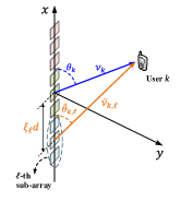
Figure 4: Illustration of the piecewise-near-field channel model.

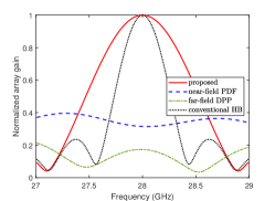
(a) $N_{\mathrm{T}}=2$.

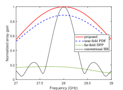
(b) $N_{\mathrm{T}}=4$.

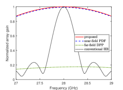
(c) $N_{\mathrm{T}}=8$.

Figure 5: Normalized array gain at the location of $(\nu_{k}=4\text{ m},\theta_{k}=60^{\circ})$ achieved by different analog beamforming schemes, where $N=256$, $f_{c}=28$ GHz, and $B=2$ GHz. Here, we assume that there is no maximum time delay constraint, i.e., $t_{\max}=\infty$.

Therefore, for the $n$-th antenna element in the $l$-th sub-array, $\forall n=0,\dots,\tilde{N}-1$, the distance to the user $k$ can be recalculated as follows, where $\chi_{\tilde{N}}^{(n)}=n-\frac{\tilde{N}-1}{2}$:

$$\bar{\nu}_{k,l,n}= \sqrt{\bar{\nu}_{k,l}^{2}+(\chi_{\tilde{N}}^{(n)})^{2}d^{2}-2\bar{\nu}_{k,l}\chi_{\tilde{N}}^{(n)}d\cos\theta_{k,l}}.$$ (48)

Next, the $n$-th entry of the array response vector $\mathbf{q}_{l}(f_{m},\theta,\nu)$ for the $l$-th sub-array at subcarrier $m$ can be rewritten as follows:

$$[\mathbf{q}_{l}(f_{m},\theta_{k},\nu_{k})]_{n}=e^{-j\frac{2\pi f_{m}}{c}(\bar{\nu}_{k,l,n}-\nu_{k})}$$

$$=e^{-j\frac{2\pi f_{m}}{c}(\bar{\nu}_{k,l}-\nu_{k})}e^{-j\frac{2\pi f_{m}}{c}(\bar{\nu}_{k,l,n}-\bar{\nu}_{k,l})}.$$ (49)

The $n$-th entry $[\mathbf{q}_{l}(f_{m},\theta_{k},\nu_{k})]_{n}$ comprises of two components: $e^{-j\frac{2\pi f_{m}}{c}(\bar{\nu}_{k,l}-r)}$ and $e^{-j\frac{2\pi f_{m}}{c}(\bar{\nu}_{k,l,n}-\bar{\nu}_{k,l})}$. The first component $e^{-j\frac{2\pi f_{m}}{c}(\bar{\nu}_{k,l}-\nu_{k})}$ represents the phase shift resulting from the difference in propagation delay between the sub-array center and the entire array center, while the second component $e^{-j\frac{2\pi f_{m}}{c}(\bar{\nu}_{k,l,n}-\bar{\nu}_{k,l})}$ represents the phase shift arising from the difference in propagation delay within the sub-array. In order to maximize the array gain at all subcarriers, the time delay $t_{k,l}$ realized the $l$-th TTD should be designed to compensate for the difference of these propagation delays. However, the propagation delay in the second component is specific to each element $n$, which is difficult to address by a common time delay $t_{k,l}$. To solve this issue, we approximate the second component $g=e^{-j\frac{2\pi f_{m}}{c}(\bar{\nu}_{k,l,n}-\bar{\nu}_{k,l})}$ as follows:

$$g= e^{-j\frac{2\pi(f_{m}-f_{c})}{c}(\bar{\nu}_{k,l,n}-\bar{\nu}_{k,l})}e^{-j\frac{2\pi f_{c}}{c}(\bar{\nu}_{k,l,n}-\bar{\nu}_{k,l})}$$

$$\approx e^{-j\frac{2\pi(f_{m}-f_{c})}{c}\eta_{k,l}}e^{-j\frac{2\pi f_{c}}{c}(\bar{\nu}_{k,l,n}-\bar{\nu}_{k,l})}$$

$$= e^{-j\frac{2\pi f_{m}}{c}\eta_{k,l}}e^{-j\frac{2\pi f_{c}}{c}\bar{\eta}_{k,l,n}},$$ (50)

where $\eta_{k,l}=\sum_{n=0}^{\tilde{N}-1}(\bar{\nu}_{k,l,n}-\bar{\nu}_{k,l})/\tilde{N}$ denote the average value of $\bar{\nu}_{k,l,n}-\bar{\nu}_{k,l}$ within a sub-array and $\bar{\eta}_{k,l,n}=\bar{\nu}_{k,l,n}-\bar{\nu}_{k,l}-\eta_{k,l}$. This approximation is reasonable because the value of $(f_{m}-f_{c})/c$ is generally relatively small. Consequently, the difference between $\bar{\nu}_{k,l,n}-\bar{\nu}_{k,l},\forall n,$ makes negligible impact. Based on the results in (V-A) and (V-A), a high-quality approximation of the piecewise-near-field array response vector $\mathbf{q}_{l}(f_{m},\theta_{k},\nu_{k})$ can be obtained, which is given by

$$\mathbf{q}_{l}(f_{m},\theta_{k},\nu_{k})\approx\boldsymbol{\beta}_{k,l}e^{-j\frac{2\pi f_{m}}{c}(\bar{\nu}_{k,l}-\nu_{k}+\eta_{k,l})},$$ (51)

where $\boldsymbol{\beta}_{k,l}=[e^{-j\frac{2\pi f_{c}}{c}\bar{\eta}_{k,l,0}},\dots,e^{-j\frac{2\pi f_{c}}{c}\bar{\eta}_{k,l,\tilde{N}-1}}]^{T}$. Then, the entire array response vector $\mathbf{b}_{N}(f_{m},\theta_{k},\nu_{k})$ can be approximated by

$$\tilde{\mathbf{a}}_{N}(f_{m},\theta_{k},\nu_{k})\triangleq\begin{bmatrix}\boldsymbol{\beta}_{k,1}e^{-j\frac{2\pi f_{m}}{c}(\bar{r}_{k,1}-\nu_{k}-\eta_{k,1})}\\[-6.00006pt] \vdots\\[-3.99994pt] \boldsymbol{\beta}_{k,N_{\mathrm{T}}}e^{-j\frac{2\pi f_{m}}{c}(\bar{r}_{k,N_{\mathrm{T}}}-\nu_{k}-\eta_{k,N_{\mathrm{T}}})}\end{bmatrix}.$$ (52)

According to (V-A), the analog beamformer $\mathbf{v}_{m,k}$ can be set to $\tilde{\mathbf{a}}_{N}^{*}(f_{m},\theta_{k},\nu_{k})e^{j\psi_{m,k}}$ to approximate the optimal beamformer. Therefore, by comparing (43) and (52), we have

$$\mathbf{a}_{k,l}e^{-j2\pi f_{m}t_{k,l}}=\boldsymbol{\beta}_{k,l}^{*}e^{j\frac{2\pi f_{m}}{c}(\bar{\nu}_{k,l}-\nu_{k}+\eta_{k,l})}e^{j\psi_{m,k}}.$$ (53)

Then, it can be readily obtained that

$$\mathbf{a}_{k,l}=\boldsymbol{\beta}_{k,l}^{*},$$ (54)

$$e^{-j2\pi f_{m}t_{k,l}}=e^{j\frac{2\pi f_{m}}{c}(\bar{\nu}_{k,l}-\nu_{k}+\eta_{k,l})}e^{j\psi_{m,k}}.$$ (55)

Since $\psi_{m}$ is an arbitrary phase, we can set it to $\psi_{m,k}=-2\pi f_{m}\vartheta_{k}$, where $\vartheta_{k}$ is an arbitrary scalar. Consequently, the second equality becomes

$$e^{-j2\pi f_{m}t_{k,l}}=e^{-j2\pi f_{m}\left(\vartheta_{k}-\frac{\bar{\nu}_{k,l}-\nu_{k}+\eta_{k,l}}{c}\right)}.\vspace{-0.2cm}$$ (56)

Let $\tilde{t}_{k,l}$ denote the unconstrained time delay. Based on the above equation, the optimal unconstrained time delay can be obtained, which is given by

$$\tilde{t}_{k,l}=\vartheta_{k}-\frac{\bar{\nu}_{k,l}-\nu_{k}+\eta_{k,l}}{c}.\vspace{-0.2cm}$$ (57)

The value of $\vartheta_{k}$ can be adjusted to make most of $\tilde{t}_{k,l},\forall l=1,\dots,N_{\mathrm{T}},$ fall in the feasible interval $[0,t_{\max}]$ of $t_{k,l}$. By defining $p_{k,l}=-(\bar{\nu}_{k,l}-\nu_{k}+\eta_{k,l})/c$, the value of $\vartheta_{k}$ can be set as follows

$$\vartheta_{k}=\frac{t_{\max}}{2}-\frac{\max_{k}p_{k,l}+\min_{k}p_{k,l}}{2}.\vspace{-0.2cm}$$ (58)

Therefore, the approximately optimal time delay of each TTD is given by

$$t_{k,l}=\max\{0,\min\{\tilde{t}_{k,l},t_{\max}\}\}.\vspace{-0.2cm}$$ (59)

The optimal analog beamformer for the sub-connected architecture can also be designed using the process outlined above. Specifically, an approximated array response vector of the sub-array connected to each RF chain is obtained in a similar manner to (52). Based on this, closed-form analog beamformers can be obtained.

There have been some existing heuristic analog beamformer designs for the TTD-based hybrid beamforming architecture, such as the near-field phase-delay focusing (PDF) approach [19] and the far-field delay-phase precoding (DPP) approach [14, 15]. In particular, the near-field PDF scheme is based on a piecewise-far-field channel model, while the far-field DPP scheme approximates the overall near-field channel by the far-field channel. However, the proposed approach relies on the exact near-field channel instead of far-field approximation and also considers the difference in propagation delay within the sub-array, resulting in higher accuracy. As shown in Fig. 5, the proposed approach achieves a higher array gain than the existing approaches, especially when the number of TTDs is not large. Additionally, in the proposed design, the maximum time delay constraint can be effectively handled, which is another novel contribution compared to the existing methods.

Algorithm 5 Proposed HTS Approach for Fully-connected Architectures.

1:  Stage I: Heuristic analog beamformer design

2:  estimate the user location information $\theta_{k}$ and $\nu_{k},\forall k,$ through near-field beam training.

3:  for  $n\in\{1,\dots,N_{\mathrm{RF}}\}$  do

4:     design the analog beamformer of the $n$-th RF chain based on user $n$’s location according to (54) and (59) if $n\leq K$. Otherwise, design it based on a random user’s location.

5:  end for

6:  Stage II: Digital beamformer optimization

7:  estimate the equivalently channel $\tilde{\mathbf{h}}_{m,k}$.

8:  optimize the digital beamformer $\mathbf{D}_{m}$ by exploiting SCA.

V-B Digital Beamformer Optimization

In the previous, a closed-form expression of the analog beamformer is derived. With the closed-form analog beamformer at hand, the received signal in (6) can be simplified as follows:

$$y_{m,k}=\tilde{\mathbf{h}}_{m,k}^{H}\mathbf{D}_{m}\mathbf{s}_{m}+n_{m,k},\vspace{-0.1cm}$$ (60)

where $\tilde{\mathbf{h}}_{m,k}=\mathbf{T}_{m}^{H}\mathbf{A}^{H}\mathbf{h}_{m,k}$ represents the equivalent channel. Since the equivalent channel has a low dimensional of $N_{\mathrm{RF}}$, it can be effectively estimated by the conventional channel estimation scheme with low complexity. Consequently, the digital beamformer can be optimized to maximize spectral efficiency with respect to the equivalent channels. The resulting optimization problem is given by

$$\max_{\mathbf{D}_{m}}\quad \sum_{m\in\mathcal{M}}\sum_{k\in\mathcal{K}}\breve{R}_{m,k}(\mathbf{D}_{m})$$ (61a)

$$\mathrm{s.t.}\quad \|\mathbf{A}\mathbf{T}_{m}\mathbf{D}_{m}\|_{F}^{2}\leq P_{t},\forall m,$$ (61b)

where

$$\breve{R}_{m,k}=\log_{2}\left(1+\frac{|\tilde{\mathbf{h}}_{m,k}^{H}\mathbf{d}_{m,k}|^{2}}{\sum_{i\in\mathcal{K},i\neq k}|\tilde{\mathbf{h}}_{m,k}^{H}\mathbf{d}_{m,i}|^{2}+\sigma_{m,k}^{2}}\right).$$ (62)

The eixsting FP, SCA, and WMMSE methods can be used to effectively solve this problem. Due to the low dimensionality of $\mathbf{D}_{m}$, the corresponding algorithm experiences low complexity. Based on the above discussion, the overall HTS approach is summarized in Algorithm 5. The HTS approach for the sub-connected architecture follows the same process, which is thus omitted here.

VI Numerical Results

In this section, numerical results obtained through Monte Carlo simulations are provided to verify the effectiveness of the proposed FAD and HTS approaches. The following simulation setup is exploited throughout our simulations unless otherwise specified. It is assumed that the BS is equipped with $N=256$ antennas with half-wavelength spacing, $N_{\mathrm{RF}}=4$ RF chains, and $N_{\mathrm{T}}=8$ TTDs for each RF chain. The maximum time delay of each TTD is set to $t_{\max}=5$ nanosecond (ns). The central frequency, system bandwidth, and number of subcarriers are assumed to be $f_{c}=28$ GHz, $B=2$ GHz, and $M=10$, respectively. There are $K=4$ near-field communication users randomly located in close proximity to the BS from $3$ m to $10$ m. The number of NLoS channels between the BS and each user is assumed to be $L_{k}=3$. The complex channel gains are generated based on the model in [27]. The noise powers of all users at all subcarriers are assumed to be the same, i.e., $\sigma_{m,k}^{2}=\sigma_{0}^{2},\forall m,k$. The SNR is defined as the ratio of the transmit power $P_{t}$ to the noise power $\sigma_{0}^{2}$, which is set to $10$ dB.

For the proposed algorithms, the convergence threshold is set to $10^{-4}$. The regularization factor $\varrho$ in Algorithm 2 is set to $\varrho=1/10$. For the penalty-based FDA approach in Algorithm 4, the penalty factor is initialized as $\rho=100$ and the reduction factor is set to $\epsilon=0.5$. Since the performance of Algorithms 2 and 3 is highly sensitive to the initialized parameters, the optimization variables of these two algorithms are initialized based on the closed-form solution obtained in the HTS approach to guarantee a good performance. For other algorithms, the optimization variables are randomly initialized within the feasible region. All following results are obtained by averaging over $100$ random channel realizations. For performance comparison, we consider both fully-digital (FD) beamforming architectures and conventional hybrid beamforming (HB) architectures as baseline schemes. In particular, the optimization of fully-digital beamformers for each subcarrier can be achieved independently by leveraging the methods in [22, 23, 24], while the optimization problems for conventional HB architectures can be effectively solved through the proposed penalty-based algorithm by setting $t_{n,l}=0$.

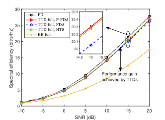
(a) Fully-connected architecture.

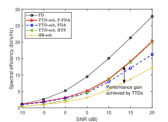
(b) Sub-connected architecture.

Figure 6: Spectral efficiency versus SNR.

In Fig. 6, we evaluate the spectral efficiency attained by different schemes versus SNR. Regarding the fully-connected architectures, as depicted in Fig. 6(a), it is evident that all the proposed approaches exhibit near-optimal performance across the entire range of SNR values under consideration due to the exploitation of TTDs, while the conventional HB approach results in significant performance degradation due to the significant near-field beam split effect. More particularly, the penalty-based FDA (P-FDA) stands out as the most effective approach due to its ability to attain a stationary point. While only exploiting part of the CSI to design the analog beamformer heuristically, the HTS approach incurs only a negligible performance loss compared to the P-FDA approach. Furthermore, the pure FDA approach is even worse than the HTS approach, as it only achieves an approximate maximization of spectral efficiency.

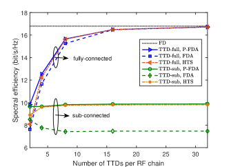
Figure 7: Spectral efficiency versus $N_{\mathrm{T}}$.

Figure 8: Energy efficiency versus $N_{\mathrm{T}}$.

Regarding the sub-connected architectures, as can be observed from Fig. 6(b), the P-FDA approach still achieves the best performance. However, it is interesting to observe that the HTS approach outperforms the FDA approach in the high SNR region, while the opposite holds true in the low SNR region. The reason behind this is explained as follows. Firstly, it is worth noting that the HTS approach for sub-connected architectures designs the analog beamformer of each sub-array for focusing on only one user. However, in the low SNR region, the objective of beamforming design is to combat the presence of significant noise. As such, each user prefers to leverage the potential of the entire antenna array to maximize the received power. Consequently, the HTS approach exhibits relatively inferior performance in such scenarios. In contrast, as the SNR increases and transitions into the high SNR region, the primary objective shifts towards mitigating inter-user interference. In this case, the HTS approach emerges as an effective strategy by dedicating the analog beamformer of each sub-array to a single user.

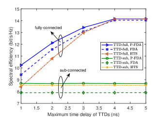
Figure 9: Spectral efficiency versus $t_{\max}$.

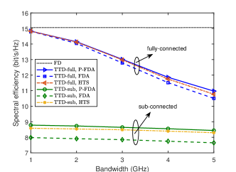
Figure 10: Spectral efficiency versus $B$.

In Fig. 7, we investigate the influence of the number of TTDs, $N_{\mathrm{T}}$, connected to each RF chain on the spectral efficiency of both fully-connected and sub-connected architectures. The results demonstrate that, as the number of TTDs increases, the performance of the fully-connected architecture, achieved through all proposed approaches, gradually converges towards the optimal fully-digital performance. This improvement is attributed to the enhanced mitigation of the near-field beam split effect achieved by incorporating additional TTDs. In contrast, in the case of sub-connected architectures, the increment in the number of TTDs has a negligible impact on the achieved spectral efficiency by the P-FDA and HTS approaches, owing to the less severe near-field beam split effect of the sub-array. This result is consistent with the analysis in Remark 1. Furthermore, when employing the FDA approach for sub-connected architectures, increasing the number of TTDs can even lead to a decrease in spectral efficiency performance. This suggests that the FDA approach becomes less accurate when a large number of TTDs are utilized in sub-connected architectures.

In Fig. 8, we further demonstrate the energy efficiency versus the number of TTDs connected to each RF chain. Energy efficiency is defined as the ratio between spectral efficiency and power consumption. In particular, let $P_{t}=100$ mW denote the transmit power, and $P_{\mathrm{BB}}=300$ mW, $P_{\mathrm{RF}}=200$ mW, $P_{\mathrm{PS}}=30$ mW, and $P_{\mathrm{TTD}}=100$ mW denote the power consumption of baseband processing, a RF chain, a PS, and a TTD, respectively [15]. Then, the power consumption of fully-digital antenna architectures is given by $P_{\mathrm{FD}}=P_{t}+P_{\mathrm{BB}}+NP_{\mathrm{RF}}$. The power consumption of the fully-connected and sub-connected TTD-based hybrid beamforming architectures is given by $P_{f}=P_{t}+P_{\mathrm{BB}}+N_{\mathrm{RF}}P_{\mathrm{RF}}+NN_{\mathrm{RF}}P_{\mathrm{PS}}+NN_{\mathrm{T}}P_{\mathrm{TTD}}$ and $P_{s}=P_{t}+P_{\mathrm{BB}}+N_{\mathrm{RF}}P_{\mathrm{RF}}+NP_{\mathrm{PS}}+NN_{\mathrm{T}}P_{\mathrm{TTD}}$, respectively. Similarly, the power consumption of conventional hybrid beamforming architectures can be calculated by excluding the power consumption attributed to TTDs. As can be observed from Fig. 8, it is evident that the energy efficiency achieved by the fully-connected architecture exhibits a peak point at $N_{\mathrm{T}}=8$. This is because, beyond this point, the additional increase in the number of TTDs leads to marginal performance improvements in spectral efficiency, as depicted in Fig. 7, while incurring a substantial power consumption. Conversely, the energy efficiency of the sub-connected architecture exhibits a continuous decline from the outset, as the installation of additional TTDs fails to provide significant improvements in spectral efficiency.

In Fig. 9, the impact of the maximum time delay $t_{\max}$ of TTDs on the performance in spectral efficiency is studied. The results demonstrate that the performance of fully-connected architectures is heavily influenced by the value of $t_{\max}$. Specifically, a minimum $t_{\max}$ of $4$ ns is required to achieve optimal performance. However, for sub-connected architectures, the minimum $t_{\max}$ that attains optimal performance is less than $1$ ns. This phenomenon can be explained as follows. In sub-connected architectures, the difference in propagation delays within each sub-array is significantly smaller compared to that of the entire array. As a result, to mitigate the near-field beam split effect for each sub-array, TTDs only need to introduce a minor time delay to compensate for the propagation delay differences. Additionally, for fully-connected architectures, the effectiveness of HTS becomes worse for the smaller $t_{\max}$. This is because, in the HTS approach, the maximum time delay constraint is simply solved by clipping, c.f., (59), rather than through optimization as in FDA approaches.

In Fig. 10, the impact of the system bandwidth $B$ on the performance in spectral efficiency is studied. The performance of fully-connected architectures experiences a notable decrease as the bandwidth increases. This is because a larger bandwidth results in a more severe near-field beam split effect, which requires more TTDs to mitigate it effectively. In contrast, sub-connected architectures exhibit only a slight performance loss with increasing bandwidth. This is also due to the small sub-array connected to each RF chain, resulting in a slight near-field beam split effect even for a large bandwidth.

VII Conclusion

In this paper, the beamfocusing optimization problem in the near-field wideband multi-user communication systems has been investigated, aiming for mitigating the performance loss caused by the near-field beam split. A new sub-connected configuration was proposed for TTD-based hybrid beamforming architectures. Three wideband beamfocusing approaches, namely the FDA, penalty-based FDA, and low-complex HTS approaches, are proposed for both fully-connected and sub-connected configurations. Numerical results showed that although the sub-connected configuration results in performance degradation in terms of spectral efficiency compared to the fully-connected configuration, it exhibits much higher energy efficiency due to the substantially reduced number of PSs and TTDs.

References

- [1] Z. Zhang et al., “6G wireless networks: Vision, requirements, architecture, and key technologies,” IEEE Veh. Technol. Mag., vol. 14, no. 3, pp. 28–41, Sep. 2019.
- [2] J. D. Kraus and R. J. Marhefka, Antennas for all applications. New York, NY, USA: McGraw-Hill, 2002.
- [3] Y. Liu et al., “Near-field communications: A tutorial review,” IEEE Open J. Commun. Soc., vol. 4, pp. 1999–2049, Aug. 2023.
- [4] R. W. Heath et al., “An overview of signal processing techniques for millimeter wave MIMO systems,” IEEE J. Sel. Topics Signal Process., vol. 10, no. 3, pp. 436–453, Apr. 2016.
- [5] H. Lu and Y. Zeng, “Near-field modeling and performance analysis for multi-user extremely large-scale MIMO communication,” IEEE Commun. Lett., vol. 26, no. 2, pp. 277–281, Feb. 2022.
- [6] H. Zhang et al., “Beam focusing for near-field multiuser MIMO communications,” IEEE Trans. Wireless Commun., vol. 21, no. 9, pp. 7476–7490, Sep. 2022.
- [7] M. Akrout et al., “Achievable rate of near-field communications based on physically consistent models,” IEEE Trans. Wireless Commun., vol. 22, no. 2, pp. 1266–1280, Feb. 2023.
- [8] G. Bacci et al., “Spherical wavefronts improve MU-MIMO spectral efficiency when using electrically large arrays,” IEEE Wireless Commun. Lett., vol. 12, no. 7, pp. 1219–1223, Jul. 2023.
- [9] R. Ji et al, “Extra DoF of near-field holographic MIMO communications leveraging evanescent waves,” IEEE Wireless Commun. Lett., vol. 12, no. 4, pp. 580–584, Apr. 2023.
- [10] B. Wang, F. Gao, S. Jin, H. Lin, and G. Y. Li, “Spatial-and frequency-wideband effects in millimeter-wave massive MIMO systems,” IEEE Trans. Signal Process., vol. 66, no. 13, pp. 3393–3406, Jul. 2018.
- [11] X. Yu et al., “Alternating minimization algorithms for hybrid precoding in millimeter wave MIMO systems,” IEEE J. Sel. Topics Signal Process., vol. 10, no. 3, pp. 485–500, Apr. 2016.
- [12] M. Cai et al., “Effect of wideband beam squint on codebook design in phased-array wireless systems,” in Proc. IEEE Global Commun. Conf. (GLOBECOM), Washington, DC, USA, Dec. 2016, pp. 1–6.
- [13] Y. Chen et al., “Hybrid precoding for wideband millimeter wave MIMO systems in the face of beam squint,” IEEE Trans. Wireless Commun., vol. 20, no. 3, pp. 1847–1860, Mar. 2021.
- [14] F. Gao, B. Wang, C. Xing, J. An, and G. Y. Li, “Wideband beamforming for hybrid massive MIMO terahertz communications,” IEEE J. Sel. Areas Commun., vol. 39, no. 6, pp. 1725–1740, Jun. 2021.
- [15] L. Dai, J. Tan, Z. Chen, and H. V. Poor, “Delay-phase precoding for wideband THz massive MIMO,” IEEE Trans. Wireless Commun., vol. 21, no. 9, pp. 7271–7286, Sep. 2022.
- [16] L. Yan et al., “Energy-efficient dynamic-subarray with fixed true-time-delay design for terahertz wideband hybrid beamforming,” IEEE J. Sel. Areas Commun., vol. 40, no. 10, pp. 2840–2854, Oct. 2022.
- [17] Z. Wang, X. Mu, J. Xu, and Y. Liu, “Simultaneously transmitting and reflecting surface (STARS) for terahertz communications,” IEEE J. Sel. Topics Signal Process., vol. 17, no. 4, pp. 861–877, Jul. 2023.
- [18] N. J. Myers and R. W. Heath, “InFocus: A spatial coding technique to mitigate misfocus in near-field LoS beamforming,” IEEE Trans. Wireless Commun., vol. 21, no. 4, pp. 2193–2209, Apr. 2022.
- [19] M. Cui, L. Dai, R. Schober, and L. Hanzo, “Near-field wideband beamforming for extremely large antenna arrays,” arXiv preprint arXiv:2109.10054, 2021.
- [20] Y. Zhang and A. Alkhateeb, “Deep learning of near field beam focusing in terahertz wideband massive MIMO systems,” IEEE Wireless Commun. Lett., vol. 12, no. 3, pp. 535–539, Mar. 2023.
- [21] O. El Ayach, S. Rajagopal, S. Abu-Surra, Z. Pi, and R. W. Heath, “Spatially sparse precoding in millimeter wave MIMO systems,” IEEE Trans. Wireless Commun., vol. 13, no. 3, pp. 1499–1513, Mar. 2014.
- [22] K. Shen and W. Yu, “Fractional programming for communication systems—part I: Power control and beamforming,” IEEE Trans. Signal Process., vol. 66, no. 10, pp. 2616–2630, May 2018.
- [23] Y. Sun, P. Babu, and D. P. Palomar, “Majorization-minimization algorithms in signal processing, communications, and machine learning,” IEEE Trans. Signal Process., vol. 65, no. 3, pp. 794–816, Feb. 2017.
- [24] S. S. Christensen et al., “Weighted sum-rate maximization using weighted MMSE for MIMO-BC beamforming design,” IEEE Trans. Wireless Commun., vol. 7, no. 12, pp. 4792–4799, Dec. 2008.
- [25] Q. Shi, M. Hong, X. Gao, E. Song, Y. Cai, and W. Xu, “Joint source-relay design for full-duplex MIMO AF relay systems,” IEEE Trans. Signal Process., vol. 64, no. 23, pp. 6118–6131, Dec. 2016.
- [26] Y. Zhang, X. Wu, and C. You, “Fast near-field beam training for extremely large-scale array,” IEEE Wireless Commun. Lett., vol. 11, no. 12, pp. 2625–2629, Dec. 2022.
- [27] M. R. Akdeniz et al., “Millimeter wave channel modeling and cellular capacity evaluation,” IEEE J. Sel. Areas Commun., vol. 32, no. 6, pp. 1164–1179, Jun. 2014.