Opinion Optimization in Directed Social Networks

Abstract

Shifting social opinions has far-reaching implications in various aspects, such as public health campaigns, product marketing, and political candidates. In this paper, we study a problem of opinion optimization based on the popular Friedkin-Johnsen (FJ) model for opinion dynamics in an unweighted directed social network with $n$ nodes and $m$ edges. In the FJ model, the internal opinion of every node lies in the closed interval $[0,1]$, with 0 and 1 being polar opposites of opinions about a certain issue. Concretely, we focus on the problem of selecting a small number of $k\ll n$ nodes and changing their internal opinions to 0, in order to minimize the average opinion at equilibrium. We then design an algorithm that returns the optimal solution to the problem in $O(n^{3})$ time. To speed up the computation, we further develop a fast algorithm by sampling spanning forests, the time complexity of which is $O(ln)$, with $l$ being the number of samplings. Finally, we execute extensive experiments on various real directed networks, which show that the effectiveness of our two algorithms is similar to each other, both of which outperform several baseline strategies of node selection. Moreover, our fast algorithm is more efficient than the first one, which is scalable to massive graphs with more than twenty million nodes.

1 Introduction

As an important part of our lives, online social networks and social media have dramatically changed the way people propagate, exchange, and formulate opinions (Ledford 2020). Increasing evidence indicates that in contrast to traditional communications and interaction, in the current digital age online communications and discussions have significantly influenced human activity in an unprecedented way, leading to universality, criticality and complexity of information propagation (Notarmuzi et al. 2022). In order to understand mechanisms for opinion propagation and shaping, a variety of mathematical models for opinion dynamics have been established (Jia et al. 2015; Proskurnikov and Tempo 2017; Dong et al. 2018; Anderson and Ye 2019). Among different models, the Friedkin-Johnsen (FJ) model (Friedkin and Johnsen 1990) is a popular one, which has been applied to many aspects (Bernardo et al. 2021; Friedkin et al. 2016). For example, the concatenated FJ model has been recently adapted to capture and reproduce the complex dynamics behind the Paris Agreement negotiation process, which explains why consensus was achieved in these multilateral international negotiations (Bernardo et al. 2021).

A fundamental quantity for opinion dynamics is the overall opinion or average opinion, which reflects the public opinions about certain topics of interest. In the past years, the subject of modifying opinions in a graph has attracted considerable attention in the scientific community (Gionis, Terzi, and Tsaparas 2013; Abebe et al. 2018; Chan, Liang, and Sozio 2019; Xu et al. 2020), since it has important implications in diverse realistic situations, such as commercial marketing, political election, and public health campaigns. For example, previous work has formulated and studied the problem of optimizing the overall or average opinion for the FJ model in undirected graphs by changing a certain attribute of some chosen nodes, including internal opinion (Xu et al. 2020), external opinion (Gionis, Terzi, and Tsaparas 2013), and susceptibility to persuasion (Abebe et al. 2018; Chan, Liang, and Sozio 2019), and so on. Thus far, most existing studies about modifying opinions focused on undirected graphs. In this paper, we study the problem of minimizing or maximizing average opinion in directed graphs (digraphs), since they can better mimic realistic networks. Moreover, because previous algorithms for unweighted graphs do not carry over to digraphs, we will propose an efficient linear-time approximation algorithm to solve the problem.

We adopt the discrete-time FJ model in a social network modeled by a digraph $\mathcal{G}=(V,E)$ with $n$ nodes and $m$ arcs. In the model, each node $i\in V$ is endowed with an internal/innate opinion $s_{i}$ in the interval $[0,1]$, where 0 and 1 are two polar opposing opinions regarding a certain topic. Moreover, each node $i\in V$ has an expressed opinion $z_{i}(t)$ at time $t$. During the opinion evolution process, the internal opinions of all nodes never change, while the expressed opinion $z_{i}(t+1)$ of any node $i$ at time $t+1$ evolves as a weighted average of $s_{i}$ and the expressed opinions of $i$’s neighbors at time $t$. For sufficiently large $t$, the expressed opinion $z_{i}(t)$ of every node $i$ converges to an equilibrium opinion $z_{i}$. We address the following optimization problem OpinionMin (or OpinionMax): Given a digraph $\mathcal{G}=(V,E)$ and a positive integer $k\ll n$, how to choose $k$ nodes and change their internal opinions to $0$ (or 1), so that the average overall steady-state opinion is minimized (or maximized).

The main contributions of our work are as follows. We formalize the problem OpinionMin (or OpinionMax) of optimizing the average equilibrium opinion by optimally selecting $k$ nodes and modifying their internal opinions to $0$ (or 1), and show that both problems are equivalent to each other. We prove that the OpinionMin problem has an optimal solution and give an exact algorithm, which returns the optimal solution in $O(n^{3})$ time. We then provide an interpretation for the average equilibrium opinion from the perspective of spanning converging forests, based on which and Wilson’s algorithm we propose a sampling based fast algorithm. The fast algorithm has an error guarantee for the main quantity concerned, and has a time complexity of $O(ln)$, where $l$ is the number of samplings. Finally, we perform extensive experiments on various real networks, which shows that our fast algorithm is almost as effective as the exact one, both outperforming several natural baselines. Furthermore, compared with the exact algorithm, our fast algorithm is more efficient, and scales to massive graphs with more than twenty million nodes.

2 Related Work

In this section, we briefly review the existing work related to ours.

Establishing mathematical models is a key step for understanding opinion dynamics and various models have been developed in the past years (Jia et al. 2015; Proskurnikov and Tempo 2017; Dong et al. 2018; Anderson and Ye 2019). Among existing models, the FJ model (Friedkin and Johnsen 1990) is a classic one, which is a significant extension of the DeGroot model (Degroot 1974). Due to its theoretical and practical significance, the FJ model has received much interest since its development. A sufficient condition for stability of the FJ model was obtained in (Ravazzi et al. 2015), its average innate opinion was inferred in (Das et al. 2013), and the vector of its expressed opinions at equilibrium was derived in (Das et al. 2013; Bindel, Kleinberg, and Oren 2015). Moreover, some explanations of the FJ model were also provided (Ghaderi and Srikant 2014; Bindel, Kleinberg, and Oren 2015). Finally, in recent years many variants or extensions of the FJ model have been introduced and studied by incorporating different factors affecting opinion formation, such as peer pressure (Semonsen et al. 2019), cooperation and competition (He et al. 2020; Xu et al. 2020), and interactions among higher-order nearest neighbors (Zhang et al. 2020).

In addition to the properties, interpretations and extensions of the FJ model itself, some social phenomena have been quantified based on the FJ model, such as disagreement (Musco, Musco, and Tsourakakis 2018), conflict (Chen, Lijffijt, and De Bie 2018), polarization (Matakos, Terzi, and Tsaparas 2017; Musco, Musco, and Tsourakakis 2018), and controversy (Chen, Lijffijt, and De Bie 2018), and a randomized algorithm approximately computing polarization and disagreement was designed in (Xu, Bao, and Zhang 2021), which was later used in (Tu and Neumann 2022). Also, many optimization problems for these quantities in the FJ model have been proposed and analyzed, including minimizing polarization (Musco, Musco, and Tsourakakis 2018; Matakos, Terzi, and Tsaparas 2017), disagreement (Musco, Musco, and Tsourakakis 2018), and conflict (Chen, Lijffijt, and De Bie 2018; Zhu and Zhang 2022), by different strategies such as modifying node’s internal opinions (Matakos, Terzi, and Tsaparas 2017), allocating edge weights (Musco, Musco, and Tsourakakis 2018) and adding edges (Zhu, Bao, and Zhang 2021). In order to solve these problems, different algorithms were designed by leveraging some mathematical tools, such as semidefinite programming (Chen, Lijffijt, and De Bie 2018) and Laplacian solvers (Zhu, Bao, and Zhang 2021).

Apart from polarization, disagreement, and conflict, another important optimization objective for opinion dynamics is the overall opinion or average opinion at equilibrium. For example, based on the FJ model, maximizing or minimizing the overall opinion has been considered by using different node-based schemes, such as changing the node’s internal opinions (Xu et al. 2020), external opinions (Gionis, Terzi, and Tsaparas 2013), and susceptibility to persuasion (Abebe et al. 2018; Chan, Liang, and Sozio 2019). On the other hand, for the DeGroot model of opinion dynamics in the presence of leaders, optimizing the overall opinion or average opinion was also heavily studied (Luca et al. 2014; Yi, Castiglia, and Patterson 2021; Zhou and Zhang 2021). An identical problem was also considered for a vote model (Yildiz et al. 2013), the asymptotic mean opinion of which is similar to that in the extended DeGroot model (Yi, Castiglia, and Patterson 2021). The vast majority of previous studies concentrated on unweighted graphs, with the exception of a few works (Ahmadinejad et al. 2015; Yi, Castiglia, and Patterson 2021), which addressed opinion optimization problems in digraphs and developed approximation algorithms with the time complexity of at least $O(n^{2.373})$. In comparison, our fast algorithm is more efficient since it has linear time complexity.

3 Preliminary

This section is devoted to a brief introduction to some useful notations and tools, in order to facilitate the description of problem formulation and algorithms.

3.1 Directed Graph and Its Laplacian Matrix

Let $\mathcal{G}=(V,E)$ denote an unweighted simple directed graph (digraph) with $n=|V|$ nodes (vertices) and $m=|E|$ directed edges (arcs), where $V=\{v_{1},v_{2},\cdots,v_{n}\}$ is the set of nodes, and $E=\{(v_{i},v_{j})\in V\times V\}$ is the set of directed edges. The existence of arc $(v_{i},v_{j})\in E$ means that there is an arc pointing from node $v_{i}$ to node $v_{j}$. In what follows, $v_{i}$ and $i$ are used interchangeably to represent node $v_{i}$ if incurring no confusion. An isolated node is a node with no arcs pointing to or coming from it. Let $N(i)$ denote the set of nodes that can be accessed by node $i$. In other words, $N(i)=\{j:(i,j)\in E\}$. A path $P$ from node $v_{1}$ to $v_{k}$ is an alternating sequence of nodes and arcs $v_{1}$,$(v_{1},v_{2})$,$v_{2}$,$\cdots$, $v_{j-1},(v_{j-1}$,$v_{j})$, $v_{j}$ in which nodes are distinct and every arc $(v_{i},v_{i+1})$ is from $v_{i}$ to $v_{i+1}$. A loop is a path plus an arc from the ending node to the starting node. A digraph is (strongly) connected if for any pair nodes $v_{x}$ and $v_{y}$, there is a path from $v_{x}$ to $v_{y}$, and there is a path from $v_{y}$ to $v_{x}$ at the same time. A digraph is called weakly connected if it is connected when one replaces any directed edge $(i,j)$ with two directed edges $(i,j)$ and $(j,i)$ in opposite directions. A tree is a weakly connected graph with no loops. An isolated node is considered as a tree. A forest is a particular graph that is a disjoint union of trees.

The connections of digraph $\mathcal{G}=(V,E)$ are encoded in its adjacency matrix $\bm{\mathit{A}}=(a_{ij})_{n\times n}$, with the element $a_{ij}$ at row $i$ and column $j$ being $1$ if $(v_{i},v_{j})\in E$ and $a_{ij}=0$ otherwise. For a node $i$ in digraph $\mathcal{G}$, its in-degree $d^{+}_{i}$ is defined as $d^{+}_{i}=\sum_{j=1}^{n}a_{ji}$, and its out-degree $d^{-}_{i}$ is defined as $d^{-}_{i}=\sum_{j=1}^{n}a_{ij}$. In the sequel, we use $d_{i}$ to represent the out-degree $d_{i}^{-}$. The diagonal out-degree matrix of digraph $\mathcal{G}$ is defined as ${\bm{\mathit{D}}}={\rm diag}(d_{1},d_{2},\ldots,d_{n})$, and the Laplacian matrix of digraph $\mathcal{G}$ is defined to be ${\bm{\mathit{L}}}={\bm{\mathit{D}}}-{\bm{\mathit{A}}}$. Let $\mathbf{1}$ and $\mathbf{0}$ be the two $n$-dimensional vectors with all entries being ones and zeros, respectively. Then, by definition, the sum of all entries in each row of $\bm{\mathit{L}}$ is equal to $0$ obeying $\bm{\mathit{L}}\mathbf{1}=\mathbf{0}$. Let $\bm{\mathit{I}}$ be the $n$-dimensional identity matrix.

In a digraph $\mathcal{G}$, if for any arc $(i,j)$, the arc $(j,i)$ exists, $\mathcal{G}$ is reduced to an undirected graph. When $\mathcal{G}$ is undirected, $a_{ij}=a_{ji}$ holds for an arbitrary pair of nodes $i$ and $j$, and thus $d^{+}_{i}=d^{-}_{i}$ holds for any node $i\in V$. Moreover, in undirected graph $\mathcal{G}$ both adjacency matrix $\bm{\mathit{A}}$ and Laplacian matrix $\bm{\mathit{L}}$ of $\mathcal{G}$ are symmetric, satisfying $\bm{\mathit{L}}\mathbf{1}=\mathbf{0}$.

3.2 Friedkin-Johnsen Model on Digraphs

The Friedkin-Johnsen (FJ) model (Friedkin and Johnsen 1990) is a popular model for opinion evolution and formation. For the FJ opinion model on a digraph $\mathcal{G}=(V,E)$, each node/agent $i\in V$ is associated with two opinions: one is the internal opinion $s_{i}$, the other is the expressed opinion $z_{i}(t)$ at time $t$. The internal opinion $s_{i}$ is in the closed interval $[0,1]$, reflecting the intrinsic position of node $i$ on a certain topic, where 0 and 1 are polar opposites of opinions regarding the topic. A higher value of $s_{i}$ signifies that node $i$ is more favorable toward the topic, and vice versa. During the process of opinion evolution, the internal opinion $s_{i}$ remains constant, while the expressed opinion $z_{i}(t)$ evolves at time $t+1$ as follows:

$$z_{i}(t+1)=\frac{s_{i}+\sum_{j\in N(i)}a_{ij}z_{j}(t)}{1+\sum_{j\in N(i)}a_{ij}}.$$ (1)

Let $\bm{\mathit{s}}=(s_{1},s_{2},\cdots,s_{n})^{\top}$ denote the vector of internal opinions, and let $\bm{\mathit{z}}(t)=(z_{1}(t),z_{2}(t),\cdots,z_{n}(t))^{\top}$ denote the vector of expressed opinions at time $t$.

Lemma 3.1

(Bindel, Kleinberg, and Oren 2015) As $t$ approaches infinity, $\bm{\mathit{z}}(t)$ converges to an equilibrium vector $\bm{\mathit{z}}=(z_{1},z_{2},\cdots,z_{n})^{\top}$ satisfying $\bm{\mathit{z}}=(\bm{\mathit{I}}+\bm{\mathit{L}})^{-1}\bm{\mathit{s}}$.

Let $\omega_{ij}$ be the element at the $i$-th row and the $j$-th column of matrix $\mathbf{\Omega}\triangleq\left(\bm{\mathit{I}}+\bm{\mathit{L}}\right)^{-1}$, which is called the fundamental matrix of the FJ model for opinion dynamics (Gionis, Terzi, and Tsaparas 2013). The fundamental matrix has many good properties (Chebotarev and Shamis 1997, 1998). It is row stochastic, since $\sum_{j=1}^{n}\omega_{ij}=1$. Moreover, $0\leq\omega_{ji}<\omega_{ii}\leq 1$ for any pair of nodes $i$ and $j$. The equality $\omega_{ji}=0$ holds if and only if $j\neq i$ and there is no path from node $j$ to node $i$; and $\omega_{ii}=1$ holds if and only if the out-degree $d_{i}$ of nodes $i$ is 0. Then, according to Lemma 3.1, for every node $i\in V$, its expressed opinion $z_{i}$ is given by $z_{i}=\sum^{n}_{j=1}\omega_{ij}s_{j}$, a convex combination of the internal opinions for all nodes.

4 Problem Formulation

An important quantity for opinion dynamics is the overall expressed opinion or the average expressed opinion at equilibrium, the optimization problem for which on the FJ model has been addressed under different constraints (Gionis, Terzi, and Tsaparas 2013; Ahmadinejad et al. 2015; Abebe et al. 2018; Xu et al. 2020; Yi, Castiglia, and Patterson 2021). In this section, we propose a problem of minimizing average expressed opinion for the FJ opinion dynamics model in a digraph, and design an exact algorithm optimally solving the problem.

4.1 Average Opinion and Structure Centrality

For the FJ model in digraph $\mathcal{G}=(V,E)$, the overall expressed opinion is defined as the sum $z_{\rm sum}$ of expressed opinions $z_{i}$ of every node $i\in V$ at equilibrium. By Lemma 3.1, $z_{i}=\sum^{n}_{j=1}\omega_{ij}s_{j}$ and $z_{\rm sum}=\sum_{i=1}^{n}z_{i}=\sum_{i=1}^{n}\sum_{j=1}^{n}\omega_{ji}s_{i}$. Given the vector for the equilibrium expressed opinions $\bm{\mathit{z}}$, we use $g(\bm{\mathit{z}})$ to denote the average expressed opinion. By definition,

$$g(\bm{\mathit{z}})=\frac{1}{n}z_{\rm sum}=\frac{1}{n}\sum_{i=1}^{n}z_{i}=\sum_{i=1}^{n}\frac{\sum_{j=1}^{n}\omega_{ji}}{n}s_{i}\,.$$ (2)

Since $g(\bm{\mathit{z}})=z_{\rm sum}/n$, related problems and algorithms for $g(\bm{\mathit{z}})$ and $z_{\rm sum}$ are equivalent to each other. In what follows, we focus on the quantity $g(\bm{\mathit{z}})$.

Equation (2) tells us that the average expressed opinion $g(\bm{\mathit{z}})$ is determined by two aspects: the internal opinion of every node, as well as the network structure characterizing interactions between nodes encoded in matrix $\mathbf{\Omega}$, both of which constitute the social structure of opinion system for the FJ model. The former is an intrinsic property of each node, while the latter is a structure property of the network, both of which together determine the opinion dynamics system. Concretely, for the equilibrium expressed opinion $z_{i}=\sum_{j=1}^{n}\omega_{ij}s_{j}$ of node $i$, $\omega_{ij}$ indicates the convex combination coefficient or contribution of the internal opinion for node $j$. And the average of the $j$-th column elements of $\mathbf{\Omega}$, denoted by $\rho_{j}\triangleq\frac{1}{n}\sum_{i=1}^{n}\omega_{ij}$, measures the contribution of the internal opinion of node $j$ to $g(\bm{\mathit{z}})$. We call $\rho_{j}$ as the structure centrality (Friedkin 2011) of node $j$ in opinion dynamics modelled by the FJ model, since it catches the long-run structure influence of node $j$ on the average expressed opinion. Note that matrix $\mathbf{\Omega}$ is row stochastic and $0\leq\omega_{ij}\leq 1$ for any pair of nodes $i$ and $j$, $0\leq\rho_{j}\leq 1$ holds for every node $j\in V$, and $\sum_{j=1}^{n}\rho_{j}=1$.

Using structure centrality, the average expressed opinion $g(\bm{\mathit{z}})$ is expressed as $g(\bm{\mathit{z}})=\sum_{i=1}^{n}\rho_{i}s_{i}$, which shows that the average expressed opinion $g(\bm{\mathit{z}})$ is a convex combination of the internal opinions of all nodes, with the weight for $s_{i}$ being the structure centrality $\rho_{i}$ of node $i$.

4.2 Problem Statement

As shown above, for a given digraph $\mathcal{G}=(V,E)$, its node centrality remains fixed. For the FJ model on $\mathcal{G}=(V,E)$ with initial vector $\bm{\mathit{s}}=(s_{1},s_{2},\cdots,s_{n})^{\top}$ of internal opinions, if we choose a set $T\subset V$ of $k$ nodes and persuade them to change their internal opinions to 0, the average equilibrium opinion, denoted by $g_{T}(\bm{\mathit{z}})$, will decrease. It is clear that for $T=\emptyset$, $g_{\emptyset}(\bm{\mathit{z}})=g(\bm{\mathit{z}})$. Moreover, for two node sets $H$ and $T$, if $T\subset H\subset V$, then $g_{T}(\bm{\mathit{z}})\geq g_{H}(\bm{\mathit{z}})$. Then the problem OpinionMin of opinion minimization arises naturally: How to optimally select a set $T$ with a small number of $k$ nodes and change their internal opinions to 0, so that their influence on the overall equilibrium opinion is maximized. Mathematically, it is formally stated as follows.

Problem 1 (OpinionMin)

Given a digraph $\mathcal{G}=(V,E)$, a vector $\bm{\mathit{s}}$ of internal opinions, and an integer $k\ll n$, we aim to find the set $T\subseteq V$ with $|T|=k$ nodes, and change the internal opinions of these chosen $k$ nodes to $0$, so that the average equilibrium opinions is minimized. That is,

$$T=\arg\min_{U\subseteq V,|U|=k}g_{U}(\bm{\mathit{z}}).$$ (3)

Similarly, we can define the problem OpinionMax for maximizing the average equilibrium opinion by optimally selecting a set $T$ of $k$ nodes and changing their internal opinions to 1. The goal of problem OpinionMin is to drive the average equilibrium opinion $g_{T}(\bm{\mathit{z}})$ towards the polar value 0, while the of goal of problem OpinionMax is to drive $g_{T}(\bm{\mathit{z}})$ towards polar value 1. Although the definitions and formulations of problems OpinionMin and OpinionMax are different, we can prove that they are equivalent to each other. In the sequel, we only consider the OpinionMin problem.

4.3 Optimal Solution

Although the OpinionMin problem is seemingly combinatorial, we next show that there is an exact algorithm optimally solving the problem in $O(n^{3})$ time.

Theorem 4.1

The optimal solution to the OpinionMin problem is the set $T$ of $k$ nodes with the largest product of structure centrality and internal opinion. That is, for any node $i\in T$ and any node $j\in V\setminus T$, $\rho_{i}s_{i}\geq\rho_{j}s_{j}$.

Proof.   Since the modifying of the internal opinions does not change the structure centrality $\rho_{i}$ of any node $i$, the optimal set $T$ of nodes for the OpinionMin problem satisfies

$$T=\arg\min_{U\subseteq V,|U|=k}\sum_{i\notin U}\rho_{i}s_{i}=\arg\max_{U\subseteq V,|U|=k}\sum_{i\in U}\rho_{i}s_{i},$$

which finishes the proof.  $\Box$

Theorem 4.1 shows that the key to solve Problem 1 is to compute $\rho_{i}$ for every node $i$. In Algorithm 1, we present an algorithm Exact, which computes $\rho_{i}$ exactly. The algorithm first computes the inverse $\mathbf{\Omega}$ of matrix $\bm{\mathit{I}}+\bm{\mathit{L}}$, which takes $O(n^{3})$ time. Based on the obtained $\mathbf{\Omega}=(\omega_{ij})_{n\times n}$, the algorithm then computes $\rho_{i}s_{i}$ for each $i\in V$ in $O(n^{2})$ time, by using the relation $\rho_{i}s_{i}=\frac{1}{n}\sum_{j=1}^{n}\omega_{ji}s_{i}$. Finally, Algorithm 1 constructs the set $T$ of $k$ nodes with the largest value of $\rho_{i}s_{i}$, which takes $O(kn)$ time. Therefore, the total time complexity of Algorithm 1 is $O(n^{3})$.

Due to the high computation complexity, Algorithm 1 is computationally infeasible for large graphs. In the next section, we will give a fast algorithm for Problem 1, which is scalable to graphs with twenty million nodes.

Input     :  A digraph $\mathcal{G}=(V,E)$; an internal opinion vector $\bm{\mathit{s}}$; an integer $k$ obeying relation $1\leq k\leq|V|$

Output :  $T$: A subset of $V$ with $|T|=k$

1 Initialize solution $T=\emptyset$

2 Compute $\mathbf{\Omega}=(\bm{\mathit{I}}+\bm{\mathit{L}})^{-1}$

3 Compute $\rho_{i}s_{i}=\frac{1}{n}\sum_{j=1}^{n}\omega_{ji}s_{i}$ for each $i\in V$

4 for $t=1$ to $k$ do

5       Select $i$ s. t. $i\leftarrow\mathrm{arg\,max}_{i\in V\setminus T}\rho_{i}s_{i}$

6       Update solution $T\leftarrow T\cup\{i\}$

7      

return $T$.

Algorithm 1 Exact$(\mathcal{G},\bm{\mathit{s}},k)$

5 Fast Sampling Algorithm

In this section, we develop a linear time algorithm to approximately evaluate the structure centrality of every node and solve the OpinionMin problem by using the connection of the fundamental matrix $\mathbf{\Omega}$ and the spanning converging forest. Our fast algorithm is based on the sampling of spanning converging forests, the ingredient of which is an extention of Wilson’s algorithm (Wilson 1996; Wilson and Propp 1996).

5.1 Interpretation of Structure Centrality

For a digraph $\mathcal{G}=(V,E)$, a spanning subgraph of $\mathcal{G}$ is a subgraph of $\mathcal{G}$ with node set being $V$ and edge set being a subset of $E$. A converging tree is a weakly connected digraph, where one node, called the root node, has out-degree 0 and all other nodes have out-degree 1. An isolated node is considered as a converging tree with the root being itself. A spanning converging forest of digraph $\mathcal{G}$ is a spanning subdigraph of $\mathcal{G}$, where all weakly connected components are converging trees. A spanning converging forest is in fact an in-forest in (Agaev and Chebotarev 2001; Chebotarev and Agaev 2002).

Let $\mathcal{F}$ be the set of all spanning converging forests of digraph $\mathcal{G}$. For a spanning converging forest $\phi\in\mathcal{F}$, let $V_{\phi}$ and $E_{\phi}$ denote its node set and arc set, respectively. By definition, for each node $i\in V_{\phi}$, there is at most one node $j\in V_{\phi}$ obeying $(i,j)\in E_{\phi}$. For a spanning converging forest $\phi$, define $\mathcal{R}(\phi)=\{i:(i,j)\notin\phi,\forall j\in V_{\phi}\}$, which is actually the set of roots of all converging trees that constitute $\phi$. Since each node $i$ in $\phi$ belongs to a certain converging tree, we define function $r_{\phi}(i):V\rightarrow\mathcal{R}(\phi)$ to map node $i$ to the root of the converging tree including $i$. Thus, if $r_{\phi}(i)=j$ we conclude that $j\in\mathcal{R}(\phi)$, and nodes $i$ and $j$ belong to the same converging tree in $\phi$. Define $\mathcal{F}_{ij}$ to be the set of those spanning converging forests, where for each spanning converging forest nodes $i$ and $j$ are in the same converging tree rooted at node $j$. That is, $\mathcal{F}_{ij}=\{\phi:r_{\phi}(i)=j,\phi\in\mathcal{F}\}$. Then, we have $\mathcal{F}_{ii}=\{\phi:i\in\mathcal{R}(\phi),\phi\in\mathcal{F}\}$.

Spanning converging forests have a close connection with the fundamental matrix of the FJ model, which is in fact the in-forest matrix of a digraph $\mathcal{G}$ introduced (Chebotarev and Shamis 1997, 1998). Using the approach in (Chaiken 1982), it is easy to derive that the entry $\omega_{ij}$ of the fundamental matrix $\mathbf{\Omega}$ can be written as $\omega_{ij}=|\mathcal{F}_{ij}|/|\mathcal{F}|$.

With the notions mentioned above, we now provide an interpretation and another expression of structure centrality $\rho_{i}$ for any node $i$. For the convenience of description, we introduce some more notations. For a node $i\in V$ and a spanning converging forest $\phi\in\mathcal{F}$ of digraph $\mathcal{G}=(V,E)$, let $M(\phi,i)$ be a set defined by $M(\phi,i)=\{j:r_{\phi}(j)=i\}$. By definition, for any $\phi\in\mathcal{F}$, if $i\notin\mathcal{R}(\phi)$, $M(\phi,i)=\emptyset$; if $i\in\mathcal{R}(\phi)$, $|M(\phi,i)|$ is equal to the number of nodes in the converging tree in $\phi$, whose root is node $i$. For two nodes $i$ and $j$ and a spanning converging forest $\phi$, define $s(\phi,j,i)$ as a function taking two values, 0 or 1:

$$s(\phi,j,i)=\begin{cases}1&\text{ if }r_{\phi}(j)=i,\\ 0&\text{ if }r_{\phi}(j)\neq i.\end{cases}$$ (4)

Then, the structure centrality $\rho_{i}$ of node $i$ is recast as

$$\rho_{i} =\frac{1}{n}\sum_{j=1}^{n}\omega_{ji}=\frac{1}{n|\mathcal{F}|}\sum_{j=1}^{n}|\mathcal{F}_{ji}|=\frac{1}{n|\mathcal{F}|}\sum\limits_{j=1}^{n}\sum\limits_{\phi\in\mathcal{F}}s(\phi,j,i)$$

$$=\frac{1}{n|\mathcal{F}|}\sum\limits_{\phi\in\mathcal{F}}\sum\limits_{j=1}^{n}s(\phi,j,i)=\frac{1}{n|\mathcal{F}|}\sum\limits_{\phi\in\mathcal{F}}|M(\phi,i)|,$$ (5)

which indicates that $\rho_{i}$ is the average number of nodes in the converging trees rooted at node $i$ in all $\phi\in\mathcal{F}$, divided by $n$.

5.2 An Expansion of Wilson’s Algorithm

We first give a brief introduction to the loop-erasure operation to a random walk (Lawler and Gregory 1980), which is a process obtained from the random walk by performing an erasure operation on its loops in chronological order. Concretely, for a random walk $P=v_{1},(v_{1},v_{2}),v_{2},\ldots,v_{k-1},(v_{j-1},v_{j}),v_{j}$, the loop-erasure $P_{\rm LE}$ to $P$ is an alternating sequence $\widetilde{v}_{1},(\widetilde{v}_{1},\widetilde{v}_{2}),\widetilde{v}_{2}\ldots,\widetilde{v}_{q-1},(\widetilde{v}_{q-1},\widetilde{v}_{q}),\widetilde{v}_{q}$ of nodes and arcs obtained inductively in the following way. First set $\widetilde{v}_{1}=v_{1}$ and append $\widetilde{v}_{1}$ to $P_{\rm LE}$. Suppose that sequence $\widetilde{v}_{1}$, $(\widetilde{v}_{1},\widetilde{v}_{2})$, $\widetilde{v}_{2}$, $\ldots$, $\widetilde{v}_{h-1}$, $(\widetilde{v}_{h-1},\widetilde{v}_{h})$, $\widetilde{v}_{h}$ has been added to $P_{\rm LE}$ for some $h\geq 1$. If $\widetilde{v}_{h}=v_{j}$, then $q=h$ and $\widetilde{v}_{h}$ is the last node in $P_{\rm LE}$. Otherwise, define $\widetilde{v}_{h+1}=v_{r+1}$, where $r=\max\{i:v_{i}=\widetilde{v}_{h}\}$.

Based on the loop-erasure operation on a random walk, Wilson proposed an algorithm to generate a uniform spanning tree rooted at a given node (Wilson 1996; Wilson and Propp 1996). Following the three steps below, we introduce Wilson’s algorithm to get a spanning tree $\tau=(V_{\tau},E_{\tau})$ of a connected digraph $\mathcal{G}=(V,E)$, which is rooted at node $u$. (i) Set $\tau=(\{u\},\emptyset)$ with $V_{\tau}=\{u\}$. Choose $i\in V\setminus V_{\tau}$. Then create an unbiased random walk starting at node $i$. At each time step, the walk jumps to a neighbor of current position with identical probability. The walk stops, when the whole walk $P$ reaches some node in $\tau$. (ii) Perform loop-erasure operation on the random walk $P$ to get $P_{\rm LE}=\widetilde{v}_{1}$, $(\widetilde{v}_{1},\widetilde{v}_{2})$, $\widetilde{v}_{2}$, $\ldots$, $(\widetilde{v}_{q-1},\widetilde{v}_{q})$, $\widetilde{v}_{q}$, and add the nodes and arcs in $P_{\rm LE}$ to $\tau$. Then update $V_{\tau}$ with the nodes in $\tau$. (iii) If $V_{\tau}\neq V$, repeat step (ii), otherwise end circulation and return $\tau$.

For a digraph $\mathcal{G}=(V,E)$, connected or disconnected, we can also apply Wilson’s Algorithm to get a spanning converging forest $\phi_{0}\in\mathcal{F}$, by using the method similar to that in (Avena and Gaudillière 2018; Pilavcı et al. 2021), which includes the following three steps. (i) We construct an augmented digraph $\mathcal{G}^{\prime}=(V^{\prime},E^{\prime})$ of $\mathcal{G}=(V,E)$, obtained from $\mathcal{G}=(V,E)$ by adding a new node $\Delta$ and some new edges. Concretely, in $\mathcal{G}^{\prime}=(V^{\prime},E^{\prime})$, $V^{\prime}=V\cup\{\Delta\}$ and $E^{\prime}=E\cup\{(i,\Delta)\}\cup\{(\Delta,i)\}$ for all $i\in V$. (ii) Using Wilson’s algorithm to generate a uniform spanning tree $\tau$ for the augmented graph $\mathcal{G}^{\prime}$, whose root node is $\Delta$. (iii) Deleting all the edges $(i,\Delta)\in\tau$ we get a spanning forest $\phi_{0}\in\mathcal{F}$ of $\mathcal{G}$. Assigning $\mathcal{R}(\phi_{0})=\{i:(i,\Delta)\in\tau\}$ as the set of roots for trees $\phi_{0}$ makes $\phi_{0}$ become a converging spanning forest of $\mathcal{G}$.

The spanning converging forest $\phi_{0}$ obtained using the above steps is uniformly selected from $\mathcal{F}$ (Avena and Gaudillière 2018). In other words, for any spanning converging forest $\phi$ in $\mathcal{F}$, we have $\mathbb{P}(\phi_{0}=\phi)=1/|\mathcal{F}|$. Following the three steps above for generating a uniform spanning converging forest of digraph $\mathcal{G}$, in Algorithm 2 we present an algorithm to generate a uniform spanning converging forest $\phi$ of digraph $\mathcal{G}$, which returns a list RootIndex with the $i$-th element RootIndex[$i$] recording the root of the tree in $\phi$ node $i$ belongs to. That is, RootIndex[$i$]=$r_{\phi}(i)$.

Input     :  $\mathcal{G}$ : a digraph

Output : RootIndex : a vector recording the root index of every node

1 InForest[$i$] $\leftarrow$ false , $i=1,2,\ldots,n$

2 Next[$i$] $\leftarrow-1$ , $i=1,2,\ldots,n$

3 RootIndex[$i$] $\leftarrow 0$, $i=1,2,\ldots,n$

4 for $i=1$ to $n$ do

5      $u\leftarrow i$

6       while not InForest[$u$] do

7             seed $\leftarrow$ Rand()

8             if seed $\leq\frac{1}{1+d_{u}}$ then

9                   InForest[$u$] $\leftarrow$ true

10                   Next[$u$]$\leftarrow-1$

11                   RootIndex[$u$] $\leftarrow u$

12                  

13            else

14                   Next[$u$] $\leftarrow$ RandomSuccessor($u,\mathcal{G}$)

15                   u $\leftarrow$ Next[$u$]

16                  

17            

18      RootNow $\leftarrow$ RootIndex[$u$]

19       $u\leftarrow i$

20       while not InForest[$u$] do

21             InForest[$u$] $\leftarrow$ true

22             RootIndex[$u$] $\leftarrow$ RootNow

23             u $\leftarrow$ Next[$u$]

24            

25      

26

27return RootIndex

Algorithm 2 $\textsc{RandomForest}(\mathcal{G})$

Below we give a detailed description for Algorithm 2. InForest is a list recording whether a node is in the forest or not in the random walk process. In line 1, we initialize InForest$[i]$ to false, for all $i\in V$. If node $i$ is not a root of any tree in the forest $\phi$, Next[$i$] is the node $j$ satisfying $(i,j)\in\phi$; if node $i$ belongs to the root set $\mathcal{R}(\phi)$, Next[$i$] $=-1$. We initialize Next[$i$] $=-1$ in line 2. We start a random walk at node $u$ in the extended graph $\mathcal{G}^{\prime}$ in line 5 to create a forest branch of $\mathcal{G}$. The probability of visiting node $\Delta$ starting from $u$ is $1/(1+d_{u})$. In line 7, we generate a random real number in $(0,1)$ using function Rand(). If the random number satisfies the inequality in line 8, the walk jumps to node $\Delta$ at this step. According to the previous analysis, in extended graph $\mathcal{G}^{\prime}$, those nodes that point directly to $\Delta$ belong to the root set $\mathcal{R}(\phi)$. In lines 9-11, we set the node $u$ as a root node and update InForest[$u$], Next$[u]$, and RootIndex$[u]$. If the inequality in line 8 does not hold, we use function RandomSuccessor($u,\mathcal{G}$) to return a node randomly selected from the neighbors of $u$ in $\mathcal{G}$ in line 13. Then we update $u$ to Next[$u$] and go back to line 6. The $\mathbf{for}$ loop stops when the random walk goes to a node already existing in the forest. When the loop stops, we get a newly created branch. In lines 15-20, we add the loop-erasure of the branch to the forest and then update RootIndex.

We now analyze the time complexity of Algorithm 2. Before doing this, we present some properties of the diagonal element $\omega_{ii}$ of matrix $\mathbf{\Omega}$ for all nodes $i\in V$.

Lemma 5.1

For any $i=1,2,\ldots,n$, the diagonal element $\omega_{ii}$ of matrix $\mathbf{\Omega}$ sastisfies $\frac{1}{1+d_{i}}\leq\omega_{ii}\leq\frac{2}{2+d_{i}}$.

Lemma 5.2

For any unweighted digraph $\mathcal{G}=(V,E)$, the expected time complexity of Algorithm 2 is $O(n)$.

Proof.   Wilson showed that the expected running time of generating a uniform spanning tree of a connected digraph $\mathcal{G}$ rooted at node $u$ is equal to a weighted average of commute time between the root and the other nodes (Wilson 1996). Marchal rewrote this average of commute time in terms of graph matrices in Proposition 1 in (Marchal 2000). According to Marchal’s result, the expected running time of Algorithm 2 is equal to the trace $\sum_{i=1}^{n}\omega_{ii}(1+d_{i})$ of matrix $\mathbf{\Omega}(\bm{\mathit{I}}+\bm{\mathit{D}})$. Using Lemma 5.2, we have $\sum_{i=1}^{n}\omega_{ii}(1+d_{i})\leq\sum_{i=1}^{n}\frac{2+2d_{i}}{2+d_{i}}\leq 2n\left(1-\frac{1}{n+1}\right).$ Thus, the expected time complexity of Algorithm 2 is $O(n)$.  $\Box$

5.3 Fast Approximation Algorithm

Here by using (5.1), we present an efficient sampling-based algorithm Fast to estimate $\rho_{i}$ for all $i\in V$ and approximately solve the problem OpinionMin in linear time.

The ingredient of the approximation algorithm Fast is the variation of Wilson’s algorithm introduced in the preceding subsection. The details of algorithm Fast are described in Algorithm 3. First, by applying Algorithm 2 we generate $l$ random spanning converging forests $\phi_{1},\phi_{2},\ldots,\phi_{l}$. Then, we compute $\widehat{\rho}_{i}=\frac{1}{nl}\sum_{j=1}^{l}|M(\phi_{j},i)|$ for all $i\in V$. Note that each of these $l$ spanning converging forests has the same probability of being created from all spanning converging forests in $\mathcal{F}$ (Avena and Gaudillière 2018). Thus, we have $\mathbb{E}\left(\frac{1}{nl}\sum_{j=1}^{l}\left|M(\phi_{j},i)\right|\right)=\rho_{i}$, which implies that $\widehat{\rho}_{i}$ in Algorithm 3 is an unbiased estimation of $\rho_{i}$. Then, $\widehat{\rho}_{i}s_{i}$ is an unbiased estimation of $\rho_{i}s_{i}$. Finally, we choose $k$ nodes from $V$ with the top-$k$ values of $\widehat{\rho}_{i}s_{i}$.

Input     : $\mathcal{G}$ : a digraph

$k$ : size of the target set

$l$ : number of generated spanning forests

Output : $\widehat{T}$ : the target set

1 Initialize : $\widehat{T}\leftarrow\emptyset$, $\widehat{\rho}_{i}\leftarrow 0,\ i=1,2,\ldots,n$

2 for $t=1$ to $l$ do

3       RootIndex $\leftarrow$ RandomForest($\mathcal{G}$)

4       for $i=1$ to $n$ do

5             $u\leftarrow$ RootIndex[$i$]

6             $\widehat{\rho}_{u}\leftarrow\widehat{\rho}_{u}+1$

7      

8$\widehat{\rho}\leftarrow\widehat{\rho}/nl$     % $\widehat{\rho}=(\widehat{\rho}_{1},\widehat{\rho}_{2},\ldots,\widehat{\rho}_{n})^{\top}$

9 for $i=1$ to $k$ do

10       $u\leftarrow\arg\max\limits_{q\in V\setminus\widehat{T}}\widehat{\rho}_{q}s_{q}$

11       $\widehat{T}\leftarrow\widehat{T}\bigcup\{u\}$

12      

13return $\widehat{T}$

Algorithm 3 $\textsc{Fast}\left(\mathcal{G},k,l\right)$

Theorem 5.3

The time complexity of Algorithm 3 is $O(ln)$.

Running Algorithm 2 requires determining the number of sampling $l$, which determines the accuracy of $\widehat{\rho}_{i}s_{i}$ as an approximation of $\rho_{i}s_{i}$. In general, the larger the value of $l$, the more accurate the estimation of $\widehat{\rho}_{i}s_{i}$ to $\rho_{i}s_{i}$. Next, we bound the number $l$ of required samplings of spanning converging forests to guarantee a desired estimation precision of $\widehat{\rho}_{i}s_{i}$ by applying the Hoeffding’s inequality (Hoeffding and Wassily 1963).

We now demonstrate that with a proper choice of $l$, $\widehat{\rho}_{i}s_{i}$ as an estimator of $\rho_{i}s_{i}$ has an approximation guarantee for all $i\in V$. Specifically, we establish an $(\epsilon,\delta)$-approximation of $\widehat{\rho}_{i}s_{i}$: for any small parameters $\epsilon>0$ and $\delta>0$, the approximation error $\widehat{\rho}_{i}s_{i}$ is bounded by $\epsilon$ with probability at least $1-\delta$. Theorem 5.4 shows how to properly choose $l$ so that $\widehat{\rho}_{i}s_{i}$ is an $(\epsilon,\delta)$-approximation of $\rho_{i}s_{i}$.

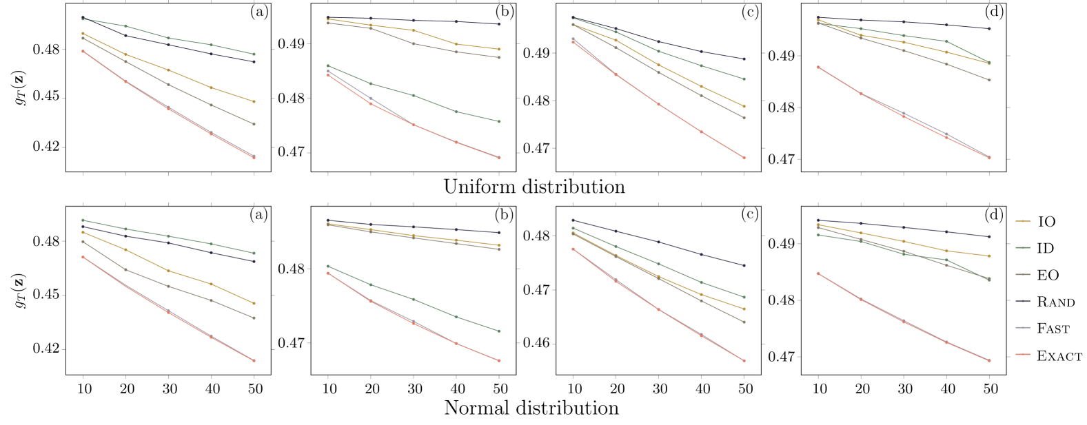
Figure 1: Average of equilibrium expressed opinions for our two algorithms Exact and Fast, and four baseline heuristics Random (Rand), In-degree (ID), Internal opinion (IO), and Expressed opinion (EO), on four directed real networks: (a) Filmtrust, (b) Dblp, (c) Humanproteins, and (d) P2p-Gnutella08.

Theorem 5.4

For any $\epsilon>0$ and $\delta\in(0,1)$, if $l$ is chosen obeying $l=\left\lceil\frac{1}{2\epsilon^{2}}\ln{\frac{2}{\delta}}\right\rceil$, then for any $i\in V$, $\mathbb{P}\left\{|\widehat{\rho}[i]s_{i}-\rho_{i}s_{i}|>\epsilon\right\}\leq\delta$.

Recall that our problem aims to determine the optimal set $T$, which consists of $k$ nodes with the largest $\rho_{i}s_{i}$. To avoid calculating $\rho_{i}$ directly, we propose a fast algorithm (Algorithm 3), which returns a set $\widehat{T}$ containing top $k$ nodes of the highest $\hat{\rho}[i]s_{i}$. Based on the result of Theorem 5.4, we can get a union bound between $g_{\widehat{T}}(\bm{\mathit{z}})$ and $g_{T}(\bm{\mathit{z}})$, as stated in the following theorem.

Theorem 5.5

For given parameters $k,\epsilon,\delta$, if $l$ is chosen according to Theorem 5.4, the inequality $|g_{\widehat{T}}(\bm{\mathit{z}})-g_{T}(\bm{\mathit{z}})|<2k\epsilon$ holds with high probability.

Proof.   According to Theorem 5.4, we suppose now inequalities $|\widehat{\rho}[i]s_{i}-\rho_{i}s_{i}|>\epsilon$ hold for any $i\in V$. Since the nodes in set $T$ have the top value of $\rho_{i}s_{i}$, we have

$$g_{\widehat{T}}(\bm{\mathit{z}})-g_{T}(\bm{\mathit{z}})=\sum_{i\notin\widehat{T}}\rho_{i}s_{i}-\sum_{i\notin T}\rho_{i}s_{i}=\sum_{i\in{T}}\rho_{i}s_{i}-\sum_{i\in\widehat{T}}\rho_{i}s_{i}\geq 0.$$

By Theorem 5.4, one obtains

$$\quad g_{\widehat{T}}(\bm{\mathit{z}})-g_{T}(\bm{\mathit{z}})\leq\sum_{i\in{T}}\widehat{\rho}[i]s_{i}-\sum_{i\in\widehat{T}}\rho_{i}s_{i}+k\epsilon$$

$$\leq\sum_{i\in\widehat{T}}\widehat{\rho}[i]s_{i}-\sum_{i\in\widehat{T}}\rho_{i}s_{i}+k\epsilon\leq 2k\epsilon,$$

which completes the proof.  $\Box$

Therefore, for any fixed $k$, the number of samples does not depend on $n$.

6 Experiments

In this section, we conduct extensive experiments on various real-life directed networks, in order to evaluate the performance of our two algorithms Exact and Fast in terms of effectiveness and efficiency. The data sets of selected real networks are publicly available in the KONECT (Kunegis 2013) and SNAP (Leskovec and Sosič 2016), the detailed information of which is presented in the first three columns of Table 1. In the dataset networks, the number $n$ of nodes ranges from about 1 thousand to 24 million, and the number $m$ of directed edges ranges from about 2 thousand to 58 million. All our experiments are programmed in Julia using a single thread, and are run on a machine equipped with 4.2 GHz Intel i7-7700 CPU and 32GB of main memory.

6.1 Effectiveness

We first compare the effectiveness of our algorithms Exact and Fast with four baseline schemes for node selection: Random, In-degree, Internal opinion, and Expressed opinion. Random selects $k$ nodes at random. In-degree chooses $k$ nodes with the largest in-degree, since a node with a high in-degree may has a strong influence on other nodes (Xu et al. 2020). For Internal opinion and Expressed opinion, they have been used in (Gionis, Terzi, and Tsaparas 2013). Internal opinion returns $k$ nodes with the largest original internal opinions, while Expressed opinion selects $k$ nodes with the largest equilibrium expressed opinions in the FJ model corresponding to the original internal opinion vector.

Network	Nodes	Arcs	Running time ($s$) for Exact and Fast				Relative error ($\times 10^{-3}$)
			Optimal	$l=500$	$l=1000$	$l=2000$	$l=500$	$l=1000$	$l=2000$
Filmtrust	874	1,853	0.023	0.019	0.037	0.042	1.08	0.55	0.11
Humanproteins	2,239	6,452	0.251	0.032	0.039	0.056	0.19	0.16	0.03
Adolescenthealth	2,539	12,969	0.354	0.034	0.068	0.134	0.72	0.59	0.09
P2p-Gnutella08	6,301	20,777	4.825	0.067	0.123	0.244	0.83	0.64	0.04
Wiki-Vote	7,115	103,689	7.405	0.078	0.156	0.312	1.13	0.87	0.13
Dblp	12,590	49,744	40.870	0.106	0.210	0.419	0.38	0.13	0.08
Wikipedialinks	17,649	296,918	110.744	0.248	0.477	0.932	1.32	0.97	0.06
Twitterlist	23,370	33,101	259.484	0.127	0.250	0.498	0.25	0.12	0.01
P2p-Gnutella31	62,586	147,892	-	0.628	1.236	2.550	-	-	-
Soc-Epinions	75,879	508,837	-	1.260	2.501	4.973	-	-	-
Email-EuAll	265,009	418,956	-	3.016	5.929	11.844	-	-	-
Stanford	281,903	2,312,500	-	7.474	14.908	29.815	-	-	-
NotreDame	325,729	1,469,680	-	4.823	9.574	19.232	-	-	-
BerkStan	685,230	7,600,600	-	14.021	28.009	56.130	-	-	-
Google	875,713	5,105,040	-	26.583	53.655	106.005	-	-	-
NorthwestUSA	1,207,940	2,820,770	-	27.758	55.509	110.410	-	-	-
WikiTalk	2,394,380	5,021,410	-	20.277	37.622	75.105	-	-	-
Greatlakes	2,758,120	6,794,810	-	64.391	128.167	255.147	-	-	-
FullUSA	23,947,300	57,708,600	-	559.147	1116.550	2230.770	-	-	-

Table 1: The running time and the relative error of Algorithms 1 and 3 on real networks for various sampling number $l$.

In our experiment, the number $l$ of samplings in algorithm Fast is set be $500$. For each node $i$, its internal opinion $s_{i}$ is generated uniformly in the interval $[0,1]$. For each real network, we first calculate the equilibrium expressed opinions of all nodes and their average opinion for the original internal opinions. Then, using our algorithms Exact and Fast and the four baseline strategies, we select $k=10,20,30,40,50$ nodes and change their internal opinions to 0, and recompute the average expressed opinion associated with the modified internal opinions. We also execute experiments for other distributions of internal opinions. For example, we consider the case that the internal opinions follow a normal distribution with mean $0$ and variance $1$. For this case, we perform a linear transformation, mapping the internal opinions into interval $[0,1]$, so that the smallest internal opinion is mapped to 0, while the largest internal opinion corresponds to 1. As can be seen from Figure 1, for each network algorithm Fast always returns a result close to the optimal solution corresponding to algorithm Exact for both uniform distribution and standardized normal distribution, outperforming the four other baseline strategies.

For the cases that internal opinions obey power-law distribution or exponential distribution, here we do not report the results since they are similar to that observed in Figure 1.

6.2 Efficiency and Scalability

As shown above, algorithm Fast has similar effectiveness to that of algorithm Exact. Below we will show that algorithm Fast is more efficient than algorithm Exact. To this end, in Table 1 we compare the performance of algorithms Exact and Fast. First, we compare the running time of the two algorithms on the real-life directed networks listed in Table 1. For our experiment, the internal opinion of all nodes in each network obeys uniform distribution from $[0,1]$, $k$ is equal to 50, and $l$ is chosen to be 500, 1000, and 2000. As shown in Table 1, Fast is significantly faster than Exact for all $l$, which becomes more obvious when the number of nodes increases. For example, Exact fails to run on the last 11 networks in Table 1, due to time and memory limitations. In contrast, Fast still works well in these networks. Particularly, algorithm Fast is scalable to massive networks with more than twenty million nodes, e.g., FullUSA with over $2.9\times 10^{7}$ nodes.

Table 1 also reports quantitative comparison of the effectiveness between algorithms Exact and Fast. Let $g_{T}$ and $g_{\widehat{T}}$ denote the average opinion obtained, respectively, by algorithms Exact and Fast, and let $\gamma=|g_{T}-g_{\widehat{T}}|/g_{T}$ be the relative error of $g_{\widehat{T}}$ with respect to $g_{T}$. The last three columns of Table 1 present the relative errors for different real networks and various numbers $l$ of samplings. From the results, we can see that for all networks and different $l$, the relative error $\gamma$ is negligible, with the largest value being less than $0.0014$. Moreover, for each network, $\gamma$ is decreased when $l$ increases. This again indicates that the results returned by Fast are very close to those corresponding to Exact. Therefore, algorithm Fast is both effective and efficient, and scales to massive graphs.

7 Conclusions

In this paper, we studied how to optimize social opinions based on the Friedkin-Johnsen (FJ) model in an unweighted directed social network with $n$ nodes and $m$ edges, where the internal opinion $s_{i}$, $i=1,2,\cdots,n$, of every node $i$ is in interval $[0,1]$. We concentrated on the problem of minimizing the average of equilibrium opinions by selecting a set $U$ of $k\ll n$ nodes and modifying their internal opinions to 0. Although the problem seems combinatorial, we proved that there is an algorithm Exact solving it in $O(n^{3})$ time, which returns the $k$ optimal nodes with the top $k$ values of $\rho_{i}s_{i}$, $i=1,\cdots,n$, where $\rho_{i}$ is the structure centrality of node $i$.

Although algorithm Exact avoids the naïve enumeration of all $\tbinom{n}{k}$ cases for set $U$, it is not applicable to large graphs. To make up for this deficiency, we proposed a fast algorithm for the problem. To this end, we provided an interpretation of $\rho_{i}$ in terms of rooted spanning converging forests, and designed a fast sampling algorithm Fast to estimate $\rho_{i}$ for all nodes by using a variant of Wilson’s Algorithm. The algorithm simultaneously returns $k$ nodes with largest values of $\rho_{i}s_{i}$ in $O(ln)$ time, where $l$ denotes the number of samplings. Finally, we performed experiments on many real directed networks of different sizes to demonstrate the performance of our algorithms. The results show that the effectiveness of algorithm Fast is comparable to that of algorithm Exact, both of which are better than the baseline algorithms. Furthermore, relative to Exact, Fast is more efficient, since is Fast is scalable to massive graphs with over twenty million nodes, while Exact only applies to graphs with less than tens of thousands of nodes. It is worth mentioning that it is easy to extend or modify our algorithm to weighed digraphs and apply it to solve other optimization problems for opinion dynamics.

References

- Abebe et al. (2018) Abebe, R.; Kleinberg, J.; Parkes, D.; and Tsourakakis, C. E. 2018. Opinion dynamics with varying susceptibility to persuasion. In Proceedings of the 24th ACM SIGKDD International Conference on Knowledge Discovery and Data Mining, 1089–1098. ACM.
- Agaev and Chebotarev (2001) Agaev, R. P.; and Chebotarev, P. Y. 2001. Spanning forests of a digraph and their applications. Automation and Remote Control, 62(3): 443–466.
- Ahmadinejad et al. (2015) Ahmadinejad, A. M.; Dehghani, S.; Hajiaghayi, M. T.; Mahini, H.; and Yazdanbod, S. 2015. Forming external behaviors by leveraging internal opinions. In Proceedings of 2015 IEEE Conference on Computer Communications, 2728–2734. IEEE.
- Anderson and Ye (2019) Anderson, B. D.; and Ye, M. 2019. Recent advances in the modelling and analysis of opinion dynamics on influence networks. International Journal of Automation and Computing, 16(2): 129–149.
- Avena and Gaudillière (2018) Avena, L.; and Gaudillière, A. 2018. Two applications of random spanning forests. Journal of Theoretical Probability, 31(4): 1975–2004.
- Bernardo et al. (2021) Bernardo, C.; Wang, L.; Vasca, F.; Hong, Y.; Shi, G.; and Altafini, C. 2021. Achieving consensus in multilateral international negotiations: The case study of the 2015 Paris Agreement on climate change. Science Advances, 7(51): eabg8068.