Quantum Parrondo Games in Low-Dimensional Hilbert Spaces

Abstract

We consider quantum variants of Parrondo games on low-dimensional Hilbert spaces. The two games which form the Parrondo game are implemented as quantum walks on a small cycle of length $M$. The dimension of the Hilbert space is $2M$. We investigate a random sequence of these two games which is realized by a quantum coin, so that the total Hilbert space dimension is $4M$. We show that in the quantum Parrondo game constructed in this way a systematic win or loss occurs in the long time limit. Due to entaglement and self-interference on the cycle, the game yields a rather complex structure for the win or loss depending on the parameters.

Keywords: Quantum games; Parrondo’s paradox; Quantum Parrondo games; Entanglement; Self-interference

1 Introduction

Since their initial description by Harmer and Abbott [1], [2] in 1999, classical Parrondo games attracted a lot of attention and many different variants have beem proposed. In all these variants, two simple fair (or losing but almost fair) games are played in some regular or random sequence leading to a systematic win. Parrondo invented these games as a simple, discrete illustration of so called Bownian motors, see [3] for a review. Other applications of Parrondo games are winning strategies in social groups [4] or by bacteriophages [5].

Quantum games have first been proposed by Meyer [6] in 1999. Already three years later, Meyer and Blumer [7] proposed quantum variants of Parrondo games based on lattice gas automata. Later, Flitney [8] proposed a different variant based on quantum walks. This approach is more natural since the original Parrondo games can be viewed as combinations of classical random walks. And their advantage compared to the initial proposal by Meyer and Blumer [7] is that they are computationally less expensive. On the other hand, and this holds for the different variants of capital dependent quantum Parrondo games presented in the review [9] by Lai and Cheong, the Parrondo effect appears as a transient effect in these games and vanishes in the infinite time limit. In contrast, Rajendran and Benjamin [10] show that if one uses two coin quantum walks, one obtains a quantum Parrondo effect in the long time limit. More recently, Panda et al. [11] show that deterministic Parrondo sequences generate highly entangled states. Recently, Walczak and Bauer [12] show that the quantum Parrondo effect occurs not only in random or deterministic periodic sequences of games but also in deterministic aperiodic sequences.

A quantum game consists of an initial state and a series of unitary transformations applied to that state. The superposition of initial states, the quantum entanglement of initial states, and quantum interference of the states induced by the unitary transformations are the three important points which make quantum games different from classical games. This holds for the quantum Parrondo games as well.

In all the realization of quantum Parrondo games by quantum walks, the games are realized using a quantum coin, i.e. an $SU(2)$ transformation of a quantum bit, which is coupled to a one-dimensional discrete walk on a line. The dimension of the Hilbert space of this combination is infinite. On the other hand, the most simple classical Parrondo game can be realized as a random walk on a cycle with length 3. The classical game on this cycle converges towards a stationary state which has a stationary, positive current. Therefore the questions arises whether it is possible to construct a quantum game using a quantum walk on a cycle of finite length, e.g. of length 3. The Hilbert space of such a game is finite, depending on the implementation it has dimension 6 or 12. This makes computations easy. Further, Tregenna et al. [13] point out that there is a fundamental difference between quantum walks on the line and on the cycle. For the latter, the interference of the quantum state with itself makes a huge difference. This might make the investigation of quantum Parrondo games on a cycle even more interesting.

The aim of this paper is to investigate quantum Parrondo games on a cycle. The paper is structured as follows: We first very briefly review classical Parrondo games on cycles. We concentrate on capital dependent games and realizations where the two different games are combined in random sequences. We then explain how these games can be realized as quantum games on cycles of length $M$. We keep this realization general, but we calculate explicit results for cycles of length $M=3$. Generalizations to larger $M$ are straight forward. Since the quantum games do not converge to a stationary state, we calculate the long time average of the current. We show that quite complex patterns for the current depending on the parameters of the game, esp. on the parameters of the quantum coin occur. We show that, depending on the parameters, the maximal current in the quantum system is larger than in the classical case and that as a function of the parameters the current changes the sign. Finally we give an outlook and propose some future research.

2 Classical Parrondo games

The original, classical Parrondo game consists of two simple games, game A and game B, typically realized by flipping biased coins, which are played in some regular or randomly alternating sequence. Since the quantum games we investigate in this paper are realized by quantum walks, we use the language of random walks for the classical games as well. In this section, we very briefly introduce the original Parrondo game, mainly to fix the notation and to compare the results for the quantum case later with the classical results.

Game A is a classical random walk on $\mathbb{Z}$. At time $t=0$ the particle starts at $x_{0}=0$. At discrete time steps $t\in\mathbb{N}$, the particle moves with probability $1/2$ one step to the left or to the right. The location of the particle after $t$ time steps is $x_{t}$. The game is fair, the expectation value of $x_{t}$ is 0. The game is even a martingale since at every step it is fair.

Game B is a modified random walk. If $x_{t}\bmod M=0$, the particle moves with probability $1/2-\epsilon_{1}$ to the right and with probability $1/2+\epsilon_{1}$ to the left. If $x_{t}\bmod M\neq 0$, the particle moves with probability $1/2+\epsilon_{2}$ to the right and with probability $1/2-\epsilon_{2}$ to the left. $\epsilon_{1,2}$ are chosen such that this game is fair as well. Fair here means that in the long time limit no systematic win or loss occurs. We will make this precise later. The original choice by Harmer and Abbott [2] was $M=3$, $\epsilon_{1}=2/5$, $\epsilon_{2}=1/4$. This game is not a martingale since the single steps are not fair. A fair game is only obtained in the stationary state. One can prove that in the long-time limit the game converges to the stationary state.

The classical Parrondo game (game C) is a random combination of game A and game B. One plays game A with probability $p_{\mathrm{A}}$ and game B with probability $p_{\mathrm{B}}=1-p_{\mathrm{A}}$. Doing so, one obtains a game which is no longer fair. The random walker moves more often in one direction than in the other. This effect is called Parrondo’s paradox.

More formally, one can treat the system as a discrete time Markov process [14] on a reduced state space $\mathbb{Z}/M\mathbb{Z}$. Let $p_{t,x}$, $x\in\mathbb{Z}/M\mathbb{Z}$ be the probability for the particle to be in state $x$ at time $t$. For the games A, B, or C the Markov process is described by a stochastic matrix $L_{\mathrm{A},\mathrm{B},\mathrm{C}}$ and

$$p_{t+1}=L_{\mathrm{A},\mathrm{B},\mathrm{C}}p_{t}$$ (1)

where $p_{t}=(p_{t,x})_{x\in\mathbb{Z}/M\mathbb{Z}}$. We have

$$L_{\mathrm{B}}=\left(\begin{array}[]{ccccc}0&1/2-\epsilon_{2}&&&1/2+\epsilon_{2}\\ 1/2-\epsilon_{1}&0&\ddots&&\\ &1/2+\epsilon_{2}&\ddots&1/2-\epsilon_{2}&\\ &&\ddots&0&1/2-\epsilon_{2}\\ 1/2+\epsilon_{1}&&&1/2+\epsilon_{2}&0\par\end{array}\right)\,,$$ (2)

the same for $L_{\mathrm{A}}$ but with $\epsilon_{1,2}=0$, and $L_{\mathrm{C}}=p_{\mathrm{A}}L_{\mathrm{A}}+p_{\mathrm{B}}L_{\mathrm{B}}$.

If $\rho$ is the stationary solution (right eigenvector of $L$ with eigenvalue 1), then let $P=\mathrm{diag}\,\rho$. The stationary current then is

$$j=LP-PL^{t}\,.$$ (3)

$j_{x,y}$ is the probability for the particle to sit on $y$ and move to $x$ minus the probability to sit on $x$ and move from $x$ to $y$. $j_{x,y}$ is therefore the net flow from $y$ to $x$. Detailled balance means $j=0$, this is the case for game A. For a fair game it is sufficient that

$$\sum_{y}j_{x,y}=0\,.$$ (4)

The parameters in game B are tuned such that it is fair. For game B with $M=3$ it is easy to show that the game is fair if $\epsilon_{1}=2\epsilon_{2}/(4\epsilon_{2}^{2}+1)$. The values $\epsilon_{1}=2/5$, $\epsilon_{2}=1/4$ chosen by Harmer and Abbott [2] clearly fulfill this condition.

Calculating the current for the combination, game C, is easy. One just needs to calculate the eigenvector of $L_{\mathrm{C}}$ and use (3). Fig. 1 shows the result for the current as a function of $p_{\mathrm{A}}$ for the original parameter set $M=3$, $\epsilon_{1}=2/5$, $\epsilon_{2}=1/4$.

Figure 1: The stationary current for $M=3$, $\epsilon_{1}=2/5$, $\epsilon_{2}=1/4$.

Since the two games A and B are fair, the current vanishes for $p_{\mathrm{A}}=0$ and $p_{\mathrm{A}}=1$. A maximum occurs near $p_{\mathrm{A}}=0.4$.

This result is well known. One can modify $M$, one can introduce different transition probabilities for the switch from game A to game B and back, one can tune $\epsilon_{1,2}$, etc. We do not go further here because our interest is to investigate a quantum version of this game.

3 Quantum Parrondo games

As an implementation for the game we use a quantum walk. It consists of a single quantum coin realized by a quantum bit and a chain (or cycle). Two unitary transformations are performed in one time step. The first is tossing the coin, the second is moving the walker along the chain depending on the result of the coin. If the walker walks on a cycle of length $M$, we need therefore a Hilbert space of dimension $2M$.

A quantum coin can be realized by elements of the (two-dimensional representation of the) Lie group $SU(2)$. We choose an arbitrary $SU(2)$ matrix. We use the parametrization

$$V(q,\phi,\theta)=\begin{pmatrix}\sqrt{q}\exp(i\phi)&\sqrt{1-q}\exp(i\theta)\\ -\sqrt{1-q}\exp(-i\theta)&\sqrt{q}\exp(-i\phi)\end{pmatrix}$$ (5)

with $0\leq q\leq 1$, $0\leq\phi\leq 2\pi$, $0\leq\theta\leq 2\pi$.

Let $J$ be a unitary transformation for a move of the walker to the right, $J^{\dagger}$ for a move to the left, and let $I$ be the identity. Let now $V\in SU(2)$ be the unitary coin tossing transformation. Let $P_{\pm}$ be the projectors onto the two states of the coin. Then

$$U_{\mathrm{A}}=(J\otimes P_{+}+J^{\dagger}\otimes P_{-})(I\otimes V)$$ (6)

represents the motion of the quantum walker. This would be the realization of game A of a Parrondo game provided the parameters are chosen such that the game is fair, esp. we need $q=1/2$ as in the classical case.

The question under which conditions $U_{\mathrm{A}}$ is unbiased (or fair) has been investigated by Tregenna et al. [13]. We reproduce their result here in a slightly modified way because we need to generalize it later when we deal with game B.

$\langle P_{\pm}\rangle$ are the expectation values for the two states of the coin. At a given time step $t$, the system is in a given state described by a density operator $\rho_{t}$.

$$\langle(P_{+}-P_{-})\rangle_{t}=\operatorname{Tr}(P_{+}-P_{-})\rho_{t}$$ (7)

yields the net flow, namely the probability to move to the right minus the probability to move to the left. We calculate this quantity for each time step and take the average over all time steps, i.e.

$$j:=\langle(P_{+}-P_{-})\rangle=\lim_{T\rightarrow\infty}\frac{1}{T}\sum_{t=1}^{T}\operatorname{Tr}(P_{+}-P_{-})\rho_{t}\,.$$ (8)

In the classical case, the long time average is identical to the stationary current calculated there because in the classical case the stochastic process converges to the stationary solution. For the quantum walk there is generically no convergence to a stationary state, therefore we take the long time average.

For a general game which is defined by a unitary transformation $U$ (take $U_{\mathrm{A}}$ as an example), we have $\rho_{t}=U^{t}\rho_{0}(U^{\dagger})^{t}$. Therefore we can calculate the trace in (8) in the eigenbasis of $U$. Let $L$ be the set of eigenvalues of $U$ and let for $\exp(i\lambda)\in L$ be $P_{\lambda}$ be the projector onto the eigenspace of the eigenvalue $\exp(i\lambda)$. Then we obtain

$$j=\sum_{\exp(i\lambda)\in L}\operatorname{Tr}((P_{+}-P_{-})P_{\lambda}\rho_{0}P_{\lambda})\,.$$ (9)

An unbiased (or fair) game is a game where $j=0$. The game is biased or unbiased with respect to a given $\rho_{0}$. There is no parameter set for which the game is unbiased for arbitrary $\rho_{0}$.

We are mainly interested in the case where $\rho_{0}$ is a pure state. But it is clearly possible to do the calculation for mixed states. If $\rho_{0}$ is proportional to the identity, we have a fully mixed state. For this case, $\rho_{t}=\rho_{0}$ and $j$ vanishes. This holds for arbitrary $U$.

The eigenbasis of $U_{\mathrm{A}}$ is easily calculated. Let $u$ be an eigenstate of $J$ to the eigenvalue $\exp(i\xi)$. Since $J$ and $J^{\dagger}$ commute, we can write the eigenstates of $U_{\mathrm{A}}$ in the form

$$\begin{pmatrix}z_{+}u\\ z_{-}u\end{pmatrix}$$ (10)

with two complex numbers $z_{\pm}$. Those are determined by the eigenvalue equation

$$\begin{pmatrix}\sqrt{q}\exp(i\phi+i\xi)&\sqrt{1-q}\exp(i\theta+i\xi)\\ -\sqrt{1-q}\exp(-i\theta-i\xi)&\sqrt{q}\exp(-i\phi-i\xi)\end{pmatrix}\begin{pmatrix}z_{+}\\ z_{-}\end{pmatrix}=\exp(i\lambda)\begin{pmatrix}z_{+}\\ z_{-}\end{pmatrix}\,.$$ (11)

For each eigenvalue $\exp(i\xi)$ of $J$ we get two eigenvalues $\exp(i\lambda)$ of $U_{\mathrm{A}}$. From the eigenvalue equation we obtain two equations for $z_{\pm}$ and those can be reduced to

$$\cos(\lambda)=\sqrt{q}\cos(\phi+\xi)$$ (12)

and

$$\sqrt{1-q}\exp(-i\theta)z_{+}=(\sqrt{q}\exp(-i\phi)-\exp(i\lambda+i\xi))z_{-}\,.$$ (13)

So far we have not been specific about the set the quantum walker is defined on. As stated and motivated in the introduction, we use a cycle. Tregenna et al. [13] point out that there is a fundamental difference between quantum walks on the line and on the cycle. For the latter, the interference of the quantum state with itself makes a huge difference. The interference is one motivation to study the games on a cycle, but more importantly, it makes the calculations cheap since the Hilbert space dimension is small for small cycles. For a cycle of length $M$ the Hilbert space dimension is $2M$ and the smallest possible value of $M$ is $M=3$.

For a cycle of length $M$ one has $J^{M}=1$ and therefore the eigenvalues of $J$ are $\exp(i\xi_{l})$ with $\xi_{l}=2\pi l/M$, $|l|\leq M/2$. For a pair of two $\xi$, $\xi^{\prime}$ for which $\xi$ and $\phi+\xi^{\prime}$ differ only by a sign, we obtain the same two values for $\lambda$ for each. Thus there may be degeneracies in the spectrum of $U_{\mathrm{A}}$.

For the concrete calculations, we use the smallest possible cycle of length $M=3$. We choose

$$\rho_{0}=\rho_{0w}\otimes\rho_{0c}$$ (14)

with

$$(\rho_{0w})_{x,y\in\mathbb{Z}/M\mathbb{Z}}=\delta_{x,y}\delta_{x,0}$$ (15)

and

$$\rho_{0c}=\frac{1}{2}\begin{pmatrix}1&\pm 1\\ \pm 1&1\end{pmatrix}\,.$$ (16)

In $\rho_{0c}$ we usually choose the upper sign, but the results we present here are independent of the sign. Note that $\rho_{0c}$ is the projection onto the state $(1,\pm 1)^{\dagger}/\sqrt{2}$, $\rho_{0}$ therefore is a density matrix of a pure state. Generalizations to mixed states are straight forward.

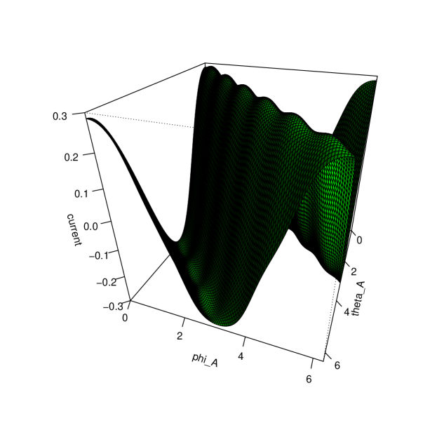
Figure 2: The time averaged current for the quantum game A, $M=3$.

In the $SU(2)$ matrix $U_{\mathrm{A}}$ which represents the quantum coin, the probability is fixed to $q_{\mathrm{A}}=1/2$ for which the classical game A is fair. The quantum game has two free parameters, the two phases $\phi_{\mathrm{A}}$ and $\theta_{\mathrm{A}}$ in the representation of the matrix $V$ in (5). The calculation of the current is easy, we just need to calculate the eigenvalues of the unitary matrix $U_{\mathrm{A}}$ and the corresponding projectors onto the eigenspaces and apply (8). The result for the current of game A as a function of the two phases $\phi_{\mathrm{A}}$ and $\theta_{\mathrm{A}}$ of $U_{\mathrm{A}}$ is shown in Fig. 2. The current vanishes for $|\theta_{\mathrm{A}}-\phi_{\mathrm{A}}|=\pi/2\bmod\pi$. One possible choice to obtain a fair game is $\phi_{\mathrm{A}}=0$ and $\theta_{\mathrm{A}}=\pi/2$. This has as well been shown in [13].

For game B of a Parrondo game we need two different unitary coin tossing transformations $V_{1,2}\in SU(2)$. Which one is used depends on the site of the walker. Let $P_{1,2}$ be the projector onto the two subsets of walker sites for which those two coin transformations are used, $P_{1}+P_{2}=I$. Then the unitary transformation for game B is

$$U_{\mathrm{B}}=(J\otimes P_{+}+J^{\dagger}\otimes P_{-})(P_{1}\otimes V_{1}+P_{2}\otimes V_{2})\,.$$ (17)

For $U_{B}$ we choose two different probabilities $q_{1}=1/2-\epsilon_{1}$ and $q_{2}=1/2+\epsilon_{2}$ for the two matrices $V_{1}$ and $V_{2}$ as in the original classical Parrondo game. We choose $M=3$ and $\rho_{0}$ as above for game A. Further we use the same phases $\phi_{\mathrm{B}}$ and $\theta_{\mathrm{B}}$ in $V_{1}$ and $V_{2}$.

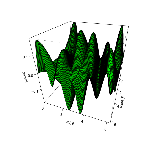
Figure 3: The time averaged current for the quantum game B, $M=3$.

The result for the current of game B as a function of the two phases $\phi_{\mathrm{B}}$ and $\theta_{\mathrm{B}}$ is shown in Fig. 3. The current vanishes for a larger set of parameters than for game A. One possible choice to obtain a fair game is $\phi_{\mathrm{B}}=0$ and $\theta_{\mathrm{B}}=\pi/2$, another possible choice is $\phi_{\mathrm{B}}=\pi/2$ and $\theta_{\mathrm{B}}=0$. For the following calculations we take the latter choice.

To obtain a Parrondo game, game A and B are played either in some regular, alternating fashion or randomly. We concentrate on the latter case, for which we need a second qbit. On the cycle, the Hilbert space dimension is then $4M$. Let $W\in SU(2)$ represent the unitary transformation for the second qbit and let $Q_{\pm}$ be the two projectors onto the two basis states of the second qbit. Then the entire unitary transformation for the quantum Parrondo game is

$$U=(U_{A}\otimes Q_{+}+U_{B}\otimes Q_{-})(I\otimes W)\,.$$ (18)

This corresponds to the classical game C. The construction is easy, $U$ consists of two unitary transformations. The first is the coin tossing represented by $W$, the second is the unitary transformation of game A or game B depending on the state of the coin. As before the current of the combined game is easily calculated by calculating the eigenvalues and the corresponding projectors of the unitary matrix $U$. We obtain generically a bias, i.e. $j\neq 0$. The value and the sign of the current depend on the parameters $q_{W}$, $\phi_{W}$ and $\theta_{W}$ in $W$ in the representation (5) and on the initial conditions. We choose the same initial condition as before in games A and B and we fix the parameters of the quantum coines in game A and B as described above, so that these two games are fair, meaning that the long time average of the current is zero. For the initial condition of the second quantum coin we take

$$\rho_{0W}=\frac{1}{2}\begin{pmatrix}1&\pm 1\\ \pm 1&1\end{pmatrix}$$ (19)

Again, we choose the upper sign. For the lower sign we obtain similar results. Then, the combined game depends on the three parameters of $W$. We first take $\theta_{W}=\pi/2$, $\phi_{W}=0$ and calculate the current as a function of $q_{W}$. The result is plotted in Fig. 4. The current is negative for very small $q$, then changes the sign and becomes positive with a maximum at $q\approx 0.2$. It then decreases, becomes negative with a maximum for $q\approx 0.9$. The current vanishes for $q=0$ and $q=1$. This must be the case since then only game A or only game B is played and both have a vanishing current.

Figure 4: The time averaged current for the combination of the two unbiased games A and B with $\theta_{\mathrm{A}}=\pi/2$, $\phi_{\mathrm{A}}=0$, $\theta_{\mathrm{B}}=0$, $\phi_{\mathrm{B}}=\pi/2$. The current is plotted as a function of the probability $q_{W}$ in the unitary transformation $W$ for the choice of game A, $\theta_{W}=\pi/2$, $\phi_{W}=0$.

We now fix $q_{W}$ and calculate the current as a function of the phases $\theta_{W}$ and $\phi_{W}$. We show the result for $q_{W}=0.2$ in Fig. 5 and the result for $q_{W}=0.8$ in Fig. 6. In both cases we see a very rich structure of the current as a function of the two phases with many sign changes, minima, and maxima. The maxima of the absolute value of the current lie above 0.1, a factor 5 higher than in the classical case.

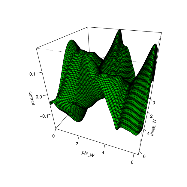
Figure 5: The time averaged current for the combination of the two unbiased games A and B with $\theta_{\mathrm{A}}=\pi/2$, $\phi_{\mathrm{A}}=0$, $\theta_{\mathrm{B}}=0$, $\phi_{\mathrm{B}}=\pi/2$. The current is plotted as a function of the two phases $\theta_{W}$ and $\phi_{W}$ and a fixed probability $q_{W}=0.2$ in the unitary transformation $W$ for the choice of game A.

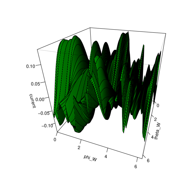
Figure 6: The time averaged current for the combination of the two unbiased games A and B with $\theta_{\mathrm{A}}=\pi/2$, $\phi_{\mathrm{A}}=0$, $\theta_{\mathrm{B}}=0$, $\phi_{\mathrm{B}}=\pi/2$. The current is plotted as a function of the two angles $\theta$ and $\phi$ and a fixed probability $q_{W}=0.8$ in the unitary transformation $W$ for the choice of game A.

The rich structure we observe here is a lot more complicated than the structure of the single games A and B depicted in Figs. 2, 3. What actually happens is the following: We have a quantum walk on a cycle which interferes with itself during its motion. Actually, this quantum walk is an $M$ state quantum system with $M=3$ in our concrete calculations. It is coupled to two quantum coins, each of dimension 2. These three quantum systems evolve in discrete time steps with a unitary transformation (18). The transformation produces a sequence of entangled states which clearly depend on the parameters of the transformation. The entanglement and the interference between of these states with themselves produce the rich structure of the long-time average of the current. This is the main result of the paper: It is possible to construct quantum Parrondo games on small Hilbert spaces, they generically show a finite current which may be positive or negative and which is larger than the classical current, and the current as a function of the parameters has a rich structure.

This is not always the case. The effect occurs for our choice of the phases of games A and B, $\theta_{\mathrm{A}}=\pi/2$, $\phi_{\mathrm{A}}=0$, $\theta_{\mathrm{B}}=0$, $\phi_{\mathrm{B}}=\pi/2$ and for many other choices for which the games A and B are fair. But there are exceptions. If instead we choose $\theta_{\mathrm{A}}=\theta_{\mathrm{B}}=\pi/2$, $\phi_{\mathrm{A}}=\phi_{\mathrm{B}}=0$, the current vanishes independent of the choice of $W$.

4 Discussion and outlook

In the classical case of game B, some fine tuning is needed to obtain a fair game. The classical games are discrete time Markov processes, for a mathematical introduction see [14]. Whereas game A is fair because it is a martingale (it is balanced at every single step), game B is not a martingale and the fairness, a vanishing current in the long-time limit, can only be assured by the fine tuning of the two probabilities involved. Combining the classical games A and B randomly, without fine tuning, leads to a current. Given the fact that already for the fairness of game B fine tuning is necessary, the occurence of a current for the random combination of games A and B is eventually less paradoxical than the term ”Parrondo’s paradox” suggests.

Quantum walks, in contrast to classical random walks, are much more complicated and do not even converge to a stationary state. Therefore, more fine tuning is needed, even for the quantum analogue of game A to obtain a fair game, a game for which the long time average of the current vanishes. A similar fine tuning is needed for game B. That the random combination of the two games is not fair, is therefore something which might have been expected. From this point of view, the inital statement of Flitney [8] that the Parrondo effect occurs only as a transient effect and vanishes in the long time limit, may look unexpected. But Flitney simply combined two simple quantum walks of the type of game A, not the quantum analogues to the classical game B. This may explain his result.

An important point to understand the results for the quantum games is the well known fact that fairness of the quantum games is not independent of the initial condition. We choose the initial condition (15) for the coin which is a pure entangled combination of the two states of the quantum coin. If one chooses as initial condition the normalized unit matrix, i.e.

$$\rho_{0c}=\frac{1}{2}\begin{pmatrix}1&0\\ 0&1\end{pmatrix}$$ (20)

which is not a pure state but the mixture of the two orthogonal pure states of the coin with equal weight, the current is always zero because any unitary transformation $V$ in (5) leaves this state invariant. In this case, there is no entanglement and no interference. In other words: If we take the average of the current for all possible different initial conditions, this should be zero. If we take the average over a subset of states, namely the states $P_{\lambda}\rho_{0}P_{\lambda}$ in (9) we may generically get non-zero values with different signs depending on the parameters which determine $P_{\lambda}$, i.e. the parameters of the unitary transformation that defines the game.

The interesting result is that the depencence of the current has an extremely rich structure as shown in Figs. 4, 5, and 6. A second, equally important result is that, depending on the parameters, the current may by much larger than in the classical case.

The rich structure we observe here certainly provokes a series of questions: Which conditions are needed for $U$ and the initial conditions to obtain the rich structure we observe and is it possible to characterize this structure in some way? Is it possible to prove that for certain conditions the current vanishes? What happens if instead of taking a random quantum choice of games A and B we play games A and B in a periodic sequence? What happens for larger values of $M$ and especially in the limit $M\rightarrow\infty$? We investigate the long time behaviour of the current, what about the transient behaviour, is it different? The early result by Flitney [8] seem to suggest that. These questions show that there is room for further research.

Another direction of research would be to investigate multi-player versions of the quantum games presented here. For multi-player versions of classical Parrondo games, interesting effects have been observed, see e.g. [15]. For the quantum version, due to the rich struture we obtain, each of the players has a huge flexibility to develop an optimal strategy.

References

- [1] Gregory Harmer and Derek Abbott. Losing strategies can win by Parrondo’s paradox. Nature 402, 864 (1999).
- [2] Derek Abbott and Gregory Harmer. Parrondo’s paradox. Statistical Science 14, 206 – 213 (1999).
- [3] P Reimann. Brownian motors: noisy transport far from equilibrium. Phys. Rep. 361, 57 (2002).
- [4] Joel Weijia Lai and Kang Hao Cheong. Social dynamics and parrondo’s paradox: a narrative review. Nonlinear Dyn 101, 1–20b (2020).
- [5] Kang Hao Cheong, Tao Wen, Sean Benler, Jin Ming Koh, and Eugene V. Koonin. Alternating lysis and lysogeny is a winning strategy in bacteriophages due to parrondo’s paradox. Proceedings of the National Academy of Sciences, 119, e2115145119 (2022).
- [6] David A. Meyer. Quantum Strategies. Phys. Rev. Lett. 82, 1052–1055 (1999).
- [7] David A. Meyer and Heather Blumer. Parrondo Games as Lattice Gas Automata. Journal of Statistical Physics 107, 225–239 (2002).
- [8] Adrian P. Flitney. Quantum Parrondo’s games using quantum walks. arxiv:1209.2252 (2012).
- [9] Joel Weijia Lai and Kang Hao Cheong. Parrondo’s paradox from classical to quantum: A review. Nonlinear Dyn 100, 849–861 (2020).
- [10] J. Rajendran and C. Benjamin. Implementing Parrondo’s paradox with two-coin quantum walks. Royal Soc. Open Sci. 5, 171599 (2018).
- [11] Dinesh Kumar Panda and B. Varun Govind and Colin Benjamin. Generating highly entangled states via discrete-time quantum walks with Parrondo sequences. Physica A 608, 128256 (2022).
- [12] Zbigniew Walczak and Jarosław H. Bauer. Parrondo’s paradox in quantum walks with deterministic aperiodic sequence of coins. Phys. Rev. E 104, 064209 (2021).
- [13] Ben Tregenna, Will Flanagan, Rik Maile, and Viv Kendon. Controlling discrete quantum walks: coins and initial states. New J. Phys. 5, 83 (2003).
- [14] Pierre Brémaud. Markov Chains. Springer Nature Switzerland AG, Cham, 2 edition, 2020.
- [15] Sandro Breuer and Andreas Mielke. Multi player parrondo games with rigid coupling. Physica A 622, 128890 (2023).