Solving Kernel Ridge Regression with Gradient-Based Optimization Methods

Abstract

Kernel ridge regression, KRR, is a generalization of linear ridge regression that is non-linear in the data, but linear in the parameters. Here, we introduce an equivalent formulation of the objective function of KRR, opening up both for using penalties other than the ridge penalty and for studying kernel ridge regression from the perspective of gradient descent. Using a continuous-time perspective, we derive a closed-form solution for solving kernel regression with gradient descent, something we refer to as kernel gradient flow, KGF, and theoretically bound the differences between KRR and KGF, where, for the latter, regularization is obtained through early stopping. We also generalize KRR by replacing the ridge penalty with the $\ell_{1}$ and $\ell_{\infty}$ penalties, respectively, and use the fact that analogous to the similarities between KGF and KRR, $\ell_{1}$ regularization and forward stagewise regression (also known as coordinate descent), and $\ell_{\infty}$ regularization and sign gradient descent, follow similar solution paths. We can thus alleviate the need for computationally heavy algorithms based on proximal gradient descent. We show theoretically and empirically how the $\ell_{1}$ and $\ell_{\infty}$ penalties, and the corresponding gradient-based optimization algorithms, produce sparse and robust kernel regression solutions, respectively.

Keywords: Kernel Ridge Regression, Gradient Descent, Forward Stagewise Regression, Sign Gradient Descent, Gradient Flow

1 Introduction

Kernel ridge regression, KRR, is a generalization of linear ridge regression that is non-linear in the data, but linear in the parameters. As for linear ridge regression, KRR has a closed-form solution, but at the cost of inverting an $n\times n$ matrix, where $n$ is the number of training observations. The KRR estimate coincides with the posterior mean of kriging, or Gaussian process regression, (Krige,, 1951; Matheron,, 1963) and has successfully been applied within a wide range of applications (Zahrt et al.,, 2019; Ali et al.,, 2020; Chen and Leclair,, 2021; Fan et al.,, 2021; Le et al.,, 2021; Safari and Rahimzadeh Arashloo,, 2021; Shahsavar et al.,, 2021; Singh Alvarado et al.,, 2021; Wu et al.,, 2021; Chen et al.,, 2022).

For linear regression, many alternatives to the ridge penalty have been proposed, including the lasso penalty (Tibshirani,, 1996), which is known for creating sparse models. By replacing the ridge penalty of KRR with the lasso penalty Roth, (2004), Guigue et al., (2005) and Feng et al., (2016) have obtained non-linear regression that is sparse in the observations. However, while the ridge penalty in KRR is formulated such that KRR can alternatively be interpreted as linear ridge regression in feature space, for these formulations the analog interpretation is lost. Rather than using the lasso, or $\ell_{1}$, penalty, Russu et al., (2016) and Demontis et al., (2017) trained kernelized support vector machines with infinity norm regularization to obtain models that are robust against adversarial data, which in the context of regression would translate to outliers. However, just as for kernelized lasso, by using their formulation, the connection to linear regression in feature space is lost.

An alternative to explicit regularization is to use an iterative optimization algorithm and stop the training before the algorithm converges. A well-known example of this is the connection between the explicitly regularized lasso model and the iterative method forward stagewise regression, which is also known as coordinate descent. The similarities between the solutions are well studied by e.g. Efron et al., (2004), Hastie et al., (2007) and Tibshirani, (2015). There are also striking similarities between explicitly regularized ridge regression and gradient descent with early stopping (Friedman and Popescu,, 2004; Ali et al.,, 2019). Replacing explicit infinity norm regularization with an iterative optimization method with early stopping does not seem to be as well studied. However, as is shown in this paper, the solutions are similar to those of sign gradient descent with early stopping.

Explicit regularization may be replaced by early stopping for different reasons, e.g. to reduce computational time. Even if closed-form solutions do exist for linear and kernel ridge regression, they include the inversion of a matrix, which is an $\mathcal{O}(d^{3})$ operation for a $\mathbb{R}^{d\times d}$ matrix, something can be avoided when by gradient descent, which has been used in the kernel setting by e.g. Yao et al., (2007), Raskutti et al., (2014) and Ma and Belkin, (2017). Moreover, while for explicit regularization this calculation has to be performed once for every considered value of the regularization strength, for an iterative optimization method, all solutions, for different stopping times, are obtained by running the algorithm to convergence just once. While the lasso and infinity norm regularized problems are still convex, in general, no closed-form solutions exist, and iterative optimization methods have to be run to convergence once for every candidate value of the regularization strength, something that tends to be computationally heavy.

In this paper, we present an equivalent formulation of KRR, which we use to obtain kernel regression with the $\ell_{1}$ and $\ell_{\infty}$ norms, in addition to the default, $\ell_{2}$, norm. We also use the equivalent formulation to solve kernel regression using the three different gradient-based optimization algorithms gradient descent, coordinate descent (forward stagewise regression), and sign gradient descent. We relate each iterative algorithm to one explicitly norm-based regularized solution and use gradient-based optimization with early stopping to obtain computationally efficient sparse, and robust, kernel regression.

The rest of the paper is structured as follows. In Section 2, we review kernel ridge regression, before introducing our equivalent formulation in Section 3. In Section 4, we review kernel gradient descent, introduce kernel gradient flow, and theoretically analyze the differences between KGF and KRR. In Section 5, we generalize KRR by replacing the $\ell_{2}$ penalty with the $\ell_{1}$ and $\ell_{\infty}$ penalties and introduce the related algorithms kernel coordinate descent and kernel sign gradient descent. Finally, in Section 6, we verify our findings with experiments on real and synthetic data.

Our main contributions are listed below.

• We present an equivalent objective function for KRR and use this formulation to generalize KRR to the $\ell_{1}$ and $\ell_{\infty}$ penalties.

• We derive a closed-form expression for kernel gradient flow, KGF, i.e. solving kernel regression with gradient descent for infinitesimal step size, and bound the differences between KGF and KRR in terms of:

  • Estimation and prediction differences.

  • Estimation and prediction risks.

• We introduce computationally efficient regularization by replacing $\ell_{1}$ and $\ell_{\infty}$ regularization by

  • kernel coordinate descent (or kernel forward stagewise regression) and

  • kernel sign gradient descent

  with early stopping. We also theoretically show that kernel coordinate descent, and kernel sign gradient descent, with early stopping, correspond to sparse and robust kernel regression, respectively.

All proofs are deferred to Appendix B.

2 Review of Kernel Ridge Regression

For a positive semi-definite kernel function, $k(\bm{x},\bm{x^{\prime}})\in\mathbb{R}$, and $n$ paired observations, $(\bm{x_{i}},y_{i})_{i=1}^{n}\in\mathbb{R}^{p}\times\mathbb{R}$, presented in a design matrix, $\bm{X}=[\bm{x_{1}}^{\top},\bm{x_{2}}^{\top},\dots\bm{x_{n}}^{\top}]^{\top}\in\mathbb{R}^{n\times p}$, and a response vector, $\bm{y}\in\mathbb{R}^{n}$, and for a given regularization strength, $\lambda>0$, the objective function of kernel ridge regression, KRR, is given by

$$\bm{\hat{\alpha}}=\operatorname*{arg\,min}_{\bm{\alpha}\in\mathbb{R}^{n}}\frac{1}{2}\left\|\bm{y}-\bm{K}\bm{\alpha}\right\|_{2}^{2}+\frac{\lambda}{2}\|\bm{\alpha}\|^{2}_{\bm{K}}$$ (1)

with predictions given by

$$\begin{bmatrix}\bm{\hat{f}}(\bm{X})\\ \bm{\hat{f}}(\bm{X^{*}})\end{bmatrix}=\begin{bmatrix}\bm{K}\\ \bm{K^{*}}\end{bmatrix}\bm{\hat{\alpha}}.$$

Here, $\bm{\hat{f}}(\bm{X})\in\mathbb{R}^{n}$ and $\bm{\hat{f}}(\bm{X^{*}})\in\mathbb{R}^{n^{*}}$ denote model predictions for the training data, $\bm{X}$, and new data, $\bm{X^{*}}=[\bm{x^{*}_{1}}{{}^{\top}},\bm{x^{*}_{2}}{{}^{\top}},\dots\bm{x^{*}_{n^{*}}}{{}^{\top}}]^{\top}\in\mathbb{R}^{n^{*}\times p}$, and $\bm{K}=\bm{K}(\bm{X})\in\mathbb{R}^{n\times n}$ and $\bm{K^{*}}=\bm{K^{*}}(\bm{X^{*}},\bm{X})\in\mathbb{R}^{n^{*}\times n}$ denote two kernel matrices defined according to $\bm{K}_{ij}=k(\bm{x_{i}},\bm{x_{j}})$ and $\bm{K^{*}}_{ij}=k(\bm{x^{*}_{i}},\bm{x_{j}})$. The weighted norm, $\|\bm{v}\|_{\bm{A}}$, is defined according to $\|\bm{v}\|_{\bm{A}}^{2}=\bm{v}^{\top}\bm{A}\bm{v}$ for any symmetric positive definite matrix $\bm{A}$.

The closed-form solution for $\bm{\hat{\alpha}}$ is given by

$$\bm{\hat{\alpha}}=\left(\bm{K}+\lambda\bm{I}\right)^{-1}\bm{y},$$ (2)

and consequently

$$\begin{bmatrix}\bm{\hat{f}}(\bm{X})\\ \bm{\hat{f}}(\bm{X^{*}})\end{bmatrix}=\begin{bmatrix}\bm{K}\\ \bm{K^{*}}\end{bmatrix}\left(\bm{K}+\lambda\bm{I}\right)^{-1}\bm{y}.$$ (3)

An alternative interpretation of KRR is as linear regression for a non-linear feature expansion of $\bm{X}$. According to Mercer’s Theorem (Mercer,, 1909), every kernel can be written as the inner product of feature expansions of its two arguments: $k(\bm{x},\bm{x^{\prime}})=\bm{\varphi}(\bm{x})^{\top}\bm{\varphi}(\bm{x^{\prime}})$ for $\bm{\varphi}(\bm{x})\in\mathbb{R}^{q}$. Thus, denoting the feature expansions of the design matrix and the new data with $\bm{\Phi}=\bm{\Phi}(\bm{X})\in\mathbb{R}^{n\times q}$ and $\bm{\Phi^{*}}=\bm{\Phi^{*}}(\bm{X^{*}})\in\mathbb{R}^{n^{*}\times q}$, the two kernel matrices can be expressed as $\bm{K}=\bm{\Phi}\bm{\Phi}^{\top}$ and $\bm{K^{*}}=\bm{\Phi^{*}}\bm{\Phi}^{\top}$. Thus, for $\bm{\beta}=\bm{\Phi}^{\top}\bm{\alpha}$, Equations 1 and 3 become

$$\bm{\hat{\beta}}=\operatorname*{arg\,min}_{\bm{\beta}\in\mathbb{R}^{q}}\frac{1}{2}\left\|\bm{y}-\bm{\Phi}\bm{\beta}\right\|_{2}^{2}+\frac{\lambda}{2}\|\bm{\beta}\|^{2}_{2}$$ (4)

$$\begin{bmatrix}\bm{\hat{f}}(\bm{X})\\ \bm{\hat{f}}(\bm{X^{*}})\end{bmatrix}=\begin{bmatrix}\bm{\Phi}\\ \bm{\Phi^{*}}\end{bmatrix}\bm{\hat{\beta}},$$

which is exactly linear ridge regression for the corresponding feature expansion.

3 Equivalent Formulations of Kernel Ridge Regression

In this section, we present an equivalent formulation of the objective function in Equation 1, which provides the same solution for $\bm{\hat{\alpha}}$ as in Equation 2. This formulation opens up for generalizing KRR by using penalties other than the ridge penalty and also provides an interesting connection to functional gradient descent (Mason et al.,, 1999).

In Appendix A, we take this one step further by reformulating Equation 1 directly in the model predictions,

$$\begin{bmatrix}\bm{f}\\ \bm{f^{*}}\end{bmatrix}:=\begin{bmatrix}\bm{f}(\bm{X})\\ \bm{f}(\bm{X^{*}})\end{bmatrix},$$

by presenting two equivalent objectives, that, when minimized with respect to $[\bm{f}^{\top},\bm{f^{*}}{{}^{\top}}]^{\top}$, generate the solution in Equation 3. In this and the following sections, all calculations are done with respect to $\bm{\alpha}$, and the corresponding expressions for $[\bm{f}^{\top},\bm{f^{*}}{{}^{\top}}]^{\top}$ are obtained through multiplication with $[\bm{K}^{\top},\bm{K^{*}}{{}^{\top}}]^{\top}$. However, in Appendix A, we show how the expressions for $[\bm{f}^{\top},\bm{f^{*}}{{}^{\top}}]^{\top}$ can alternatively be obtained directly without taking the detour over $\bm{\alpha}$.

In Lemma 1, we show how we can move the weighted norm in Equation 1 from the penalty term to the reconstruction term.

Lemma 1.

$$\bm{\hat{\alpha}}= \operatorname*{arg\,min}_{\bm{\alpha}\in\mathbb{R}^{n}}\frac{1}{2}\left\|\bm{y}-\bm{K}\bm{\alpha}\right\|_{2}^{2}+\frac{\lambda}{2}\|\bm{\alpha}\|^{2}_{\bm{K}}$$ (5a)

$$= \operatorname*{arg\,min}_{\bm{\alpha}\in\mathbb{R}^{n}}\frac{1}{2}\left\|\bm{y}-\bm{K}\bm{\alpha}\right\|_{\bm{K}^{-1}}^{2}+\frac{\lambda}{2}\|\bm{\alpha}\|^{2}_{2}$$ (5b)

$$= \left(\bm{K}+\lambda\bm{I}\right)^{-1}\bm{y}.$$

The alternative formulation in Equation 5b, where the reconstruction term rather than the regularization term, is weighted by the kernel matrix, has two interesting implications. First, a standard ridge penalty on the regularization term opens up for using other penalties than the $\ell_{2}$ norm, such as the $\ell_{1}$ and $\ell_{\infty}$ norms. Although these penalties have previously been used in the kernel setting, it has been done by replacing $\|\bm{\alpha}\|_{\bm{K}}^{2}$ in Equation 1 by $\|\bm{\alpha}\|_{1}$ or $\|\bm{\alpha}\|_{\infty}$, thus ignoring the impact of $\bm{K}$, by acting as if the objective of KRR were to minimize $\|\bm{y}-\bm{K}\bm{\alpha}\|_{2}^{2}+\lambda\|\bm{\alpha}\|_{2}^{2}$. This form has the solution $\bm{\hat{\alpha}}=\bm{K}(\bm{K}^{2}+\lambda)^{-1}\bm{y}$, for which the connection to linear regression in feature space is lost.

Second, the gradient of Equation 5b with respect to $\bm{\alpha}$ is

$$\bm{K}\bm{\alpha}-\bm{y}+\lambda\bm{\alpha}$$ (6)

Multiplying by $[\bm{K}^{\top},\bm{K^{*}}{{}^{\top}}]^{\top}$, we obtain

$$\begin{bmatrix}\bm{K}\\ \bm{K^{*}}\end{bmatrix}(\bm{f}-\bm{y})+\lambda\begin{bmatrix}\bm{f}\\ \bm{f^{*}}\end{bmatrix},$$ (7)

which is the gradient used in functional gradient descent, where it is obtained from differentiating functionals. Here, however, it is a simple simple consequence of the equivalent objective function of KRR.

4 Kernel Gradient Descent and Kernel Gradient Flow

In this section, we investigate solving kernel regression iteratively with gradient descent. We also use gradient descent with infinitesimal step size, known as gradient flow, to obtain a closed-form solution which we use for direct comparisons to kernel ridge regression.

The similarities between ridge regression and gradient descent with early stopping are well studied for linear regression (Friedman and Popescu,, 2004; Ali et al.,, 2019; Allerbo et al.,, 2023). When starting at zero, optimization time can be thought of as an inverse penalty, where longer optimization time corresponds to weaker regularization. When applying gradient descent to kernel regression, something we refer to as kernel gradient descent, KGD, we will replace explicit regularization with implicit regularization through early stopping. That is, we will use $\lambda=0$ and consider training time, $t$, as a regularizer.

With $\lambda=0$ in Equation 6, starting at $\bm{0}$, the KGD update becomes, for step size $\eta$,

$$\bm{\hat{\alpha}}_{k+1}=\bm{\hat{\alpha}}_{k}+\eta\cdot\left(\bm{y}-\bm{K}\bm{\hat{\alpha}}_{k}\right),\ \bm{\hat{\alpha}}_{0}=\bm{0}.$$ (8)

To compare the regularization injected by early stopping to that of ridge regression, we let the optimization step size go to zero to obtain a closed-form solution, which we refer to as kernel gradient flow, KGF. Then, Equation 8 can be thought of as the Euler forward formulation of the differential equation in Equation 9,

$$\frac{d\bm{\hat{\alpha}}(t)}{dt}=\bm{y}-\bm{K}\bm{\hat{\alpha}}(t),\ \bm{\hat{\alpha}}(0)=\bm{0}$$ (9)

whose solution is stated in Lemma 2.

Lemma 2.

The solution to the differential equation in Equation 9 is

$$\bm{\hat{\alpha}}(t)=(\bm{I}-\exp(-t\bm{K}))\bm{K}^{-1}\bm{y}=:\bm{\hat{\alpha}}_{\text{KGF}}(t),$$ (10)

where $\exp$ denotes the matrix exponential.

Remark 1: Note that $(\bm{I}-\exp(-t\bm{K}))\bm{K}^{-1}=\bm{K}^{-1}(\bm{I}-\exp(-t\bm{K}))$ is well-defined even if $\bm{K}$ is singular. The matrix exponential is defined through its Taylor approximation and from $\bm{I}-\exp(-t\bm{K})=t\bm{K}-\frac{1}{2!}t^{2}\bm{K}^{2}+\dots$, a matrix $\bm{K}$ factors out, that cancels with $\bm{K}^{-1}$.
Remark 2: It is possible to generalize Lemma 2 to Nesterov accelerated gradient descent with momentum (Nesterov,, 1983; Polyak,, 1964). In this case $\exp(-t\bm{K})$ in Equation 10 generalizes to $\exp\left(-\frac{t}{1-\gamma}\bm{K}\right)$, where $\gamma\in[0,1)$ is the strength of the momentum. See the proof in the appendix for details.

To facilitate the comparisons between KGF and KRR, we rewrite Equation 2 using Lemma 3, from which we obtain

$$\bm{\hat{\alpha}}_{\text{KRR}}(\lambda)=\left(\bm{I}-\left(\bm{I}+1/\lambda\cdot\bm{K}\right)^{-1}\right)\bm{K}^{-1}\bm{y}.$$ (11)

Since $\exp(-t\bm{K})=\exp(t\bm{K})^{-1}$, the KGF and KRR solutions differ only in the factor

$$\exp(t\bm{K})\text{ v.s. }\bm{I}+1/\lambda\bm{K}.$$ (12)

Thus, for $t=1/\lambda$, we can think of the ridge penalty as a first-order Taylor approximation of the gradient flow penalty, where, since $e^{tk}\geq 1+tk$, the KGF solution tends to lie closer to the observations than the KRR solution does.

Lemma 3.

$$\left(\bm{K}+\lambda\bm{I}\right)^{-1}=\left(\bm{I}-\left(\bm{I}+1/\lambda\cdot\bm{K}\right)^{-1}\right)\bm{K}^{-1}.$$

4.1 Comparisons between Kernel Ridge Regression and Kernel Gradient Flow

In this section, we compare the KRR and KGF solutions for $\lambda=1/t$. To do this, we introduce the following notation, where $\bm{k}(\bm{x^{*}})^{\top}=\bm{k}(\bm{x^{*}},\bm{X})^{\top}\in\mathbb{R}^{n}$ is the row in $\bm{K^{*}}$ corresponding to $\bm{x^{*}}$:

$$\bm{\hat{f}}_{\text{KGF}}(\bm{X},t):=\bm{K}\bm{\hat{\alpha}}_{\text{KGF}}(t),\quad\hat{f}_{\text{KGF}}(\bm{x^{*}},t):=\bm{k}(\bm{x^{*}})^{\top}\bm{\hat{\alpha}}_{\text{KGF}}(t),$$

$$\bm{\hat{f}}_{\text{KRR}}(\bm{X},\lambda):=\bm{K}\bm{\hat{\alpha}}_{\text{KRR}}(\lambda),\quad\hat{f}_{\text{KRR}}(\bm{x^{*}},\lambda):=\bm{k}(\bm{x^{*}})^{\top}\bm{\hat{\alpha}}_{\text{KRR}}(\lambda),$$

$$\bm{\hat{\alpha}}^{0}:=\bm{\hat{\alpha}}_{\text{KGF}}(t=\infty)=\bm{\hat{\alpha}}_{\text{KRR}}(\lambda=0)=\bm{K}^{-1}\bm{y},$$

$$\bm{\hat{f}}^{0}(\bm{X}):=\bm{\hat{f}}_{\text{KGF}}(\bm{X},t=\infty)=\bm{\hat{f}}_{\text{KRR}}(\bm{X},\lambda=0)=\bm{K}\bm{\hat{\alpha}}^{0}=\bm{y},$$

$$\hat{f}^{0}(\bm{x^{*}}):=\hat{f}_{\text{KGF}}(\bm{x^{*}},t=\infty)=\hat{f}_{\text{KRR}}(\bm{x^{*}},\lambda=0)=\bm{k}(\bm{x^{*}})^{\top}\bm{\hat{\alpha}}^{0}=\bm{k}(\bm{x^{*}})^{\top}\bm{K}^{-1}\bm{y},$$

$$\hat{\alpha}_{i}^{\text{KGF}}:=(\bm{\hat{\alpha}}_{\text{KGF}})_{i},\quad\hat{\alpha}_{i}^{\text{KRR}}:=(\bm{\hat{\alpha}}_{\text{KRR}})_{i},\quad\hat{\alpha}_{i}^{0}:=(\bm{\hat{\alpha}}^{0})_{i}.$$

In Proposition 1, we bound the differences between the KGF and KRR solutions in terms of the non-regularized solutions, $\bm{\alpha_{0}}$, $\bm{\hat{f}}^{0}(\bm{X})$ and $\hat{f}^{0}(\bm{x^{*}})$. In parts (a) and (b), where the difference between the parameter and in-sample prediction vectors are bounded, no further assumptions are needed. In parts (c) and (d), with bounds on individual parameters and predictions, including out-of-sample predictions, some very reasonable assumptions have to be made on the data. For all four bounds, the larger the non-regularized value is, the larger the difference between the KGF and KRR estimates is allowed to be.

Proposition 1.

For $t\geq 0$,

• $\left\|\bm{\hat{\alpha}}_{\text{KGF}}(t)-\bm{\hat{\alpha}}_{\text{KRR}}(1/t)\right\|_{2}^{2}\leq 0.0415\cdot\|\bm{\hat{\alpha}}^{0}\|_{2}^{2}$,

• $\left\|\bm{\hat{f}}_{\text{KGF}}(\bm{X},t)-\bm{\hat{f}}_{\text{KRR}}(\bm{X},1/t)\right\|_{2}^{2}\leq 0.0415\cdot\|\bm{\hat{f}}^{0}(\bm{X})\|_{2}^{2}=0.0415\cdot\|\bm{y}\|_{2}^{2}$.

For $\bm{y}=\bm{K}\bm{\alpha_{0}}+\bm{\varepsilon},\ \bm{\alpha_{0}}\sim(\bm{0},\bm{\Sigma_{\alpha}}),\ \bm{\varepsilon}\sim(\bm{0},\sigma_{\varepsilon}^{2}\bm{I})$, where $\bm{\Sigma_{\alpha}}$ and $\bm{K}$ are simultaneously diagonalizable,

• $\mathbb{E}_{\bm{\varepsilon},\bm{\alpha_{0}}}\left(\left(\hat{\alpha}_{i}^{\text{KGF}}(t)-\hat{\alpha}_{i}^{\text{KRR}}(1/t)\right)^{2}\right)\leq 0.0415\cdot\mathbb{E}_{\bm{\varepsilon},\bm{\alpha_{0}}}\left((\hat{\alpha}_{i}^{0})^{2}\right)$, $i=1,2,\dots n$,

• $\mathbb{E}_{\bm{\varepsilon},\bm{\alpha_{0}}}\left(\left(\hat{f}_{\text{KGF}}(\bm{x^{*}},t)-\hat{f}_{\text{KRR}}(\bm{x^{*}},1/t)\right)^{2}\right)\leq 0.0415\cdot\mathbb{E}_{\bm{\varepsilon},\bm{\alpha_{0}}}\left(\hat{f}^{0}(\bm{x^{*}})^{2}\right)$.

Two typical options for $\bm{\Sigma_{\alpha}}$ are $\sigma_{\alpha}^{2}\bm{I}$ and $\sigma_{\beta}^{2}\bm{K}^{-1}$, where the second formulation implies $\bm{\beta_{0}}\sim(\bm{0},\sigma_{\beta}^{2}\bm{I})$ in the feature space formulation of KRR from Equation 4.

If we assume that a true function exists, parameterized by the true $\bm{\alpha_{0}}$ as

$$\begin{bmatrix}\bm{f_{0}}(\bm{X})\\ \bm{f_{0}}(\bm{X^{*}})\end{bmatrix}=\begin{bmatrix}\bm{K}\\ \bm{K^{*}}\end{bmatrix}\bm{\alpha_{0}},$$

and with observations according to $\bm{y}=\bm{f_{0}}(\bm{X})+\bm{\varepsilon}$, we can calculate the expected squared differences between the estimated and true models, something that is often referred to as the risk: $\text{Risk}(\bm{\hat{\theta}};\bm{\theta_{0}})=\mathbb{E}\left(\|\bm{\hat{\theta}}-\bm{\theta_{0}}\|_{2}^{2}\right)$. In Proposition 2, the KGF estimation and prediction risks are bounded in terms of the corresponding KRR risks. In all three cases, the KGF risk is less than 1.69 times the KRR risk.

Proposition 2.

For $t\geq 0$, $\bm{y}=\bm{f_{0}}(\bm{X})+\bm{\varepsilon}=\bm{K}\bm{\alpha_{0}}+\bm{\varepsilon}$, $\bm{\varepsilon}\sim(\bm{0},\sigma_{\varepsilon}^{2}\bm{I})$,

• For any $\bm{\alpha_{0}}$, $\text{\emph{Risk}}(\bm{\hat{\alpha}}_{\text{KGF}}(t);\bm{\alpha_{0}})\leq 1.6862\cdot\text{\emph{Risk}}(\bm{\hat{\alpha}}_{\text{KRR}}(1/t);\bm{\alpha_{0}})$.

• For any $\bm{\alpha_{0}}$, $\text{\emph{Risk}}(\bm{\hat{f}}_{\text{KGF}}(\bm{X},t);\bm{f_{0}}(\bm{X}))\leq 1.6862\cdot\text{\emph{Risk}}(\bm{\hat{f}}_{\text{KRR}}(\bm{X},1/t);\bm{f_{0}}(\bm{X}))$.

• For $\bm{\alpha_{0}}\sim\left(\bm{0},\bm{\Sigma_{\alpha}}\right)$, where $\bm{\Sigma_{\alpha}}$ and $\bm{K}$ are simultaneously diagonalizable,
  $\mathbb{E}_{\bm{\alpha_{0}}}\left(\text{\emph{Risk}}(\hat{f}_{\text{KGF}}(\bm{x^{*}},t);f_{0}(\bm{x^{*}}))\right)\leq 1.6862\cdot\mathbb{E}_{\bm{\alpha_{0}}}\left(\text{\emph{Risk}}(\hat{f}_{\text{KRR}}(\bm{x^{*}},1/t);f_{0}(\bm{x^{*}}))\right)$,
  where $f_{0}(\bm{x^{*}})\in\bm{f_{0}}(\bm{X^{*}})$.

5 Kernel Regression with the $\ell_{1}$ and $\ell_{\infty}$ Norms

In this section, we replace the squared $\ell_{2}$ norm of KRR in Equation 5b by the $\ell_{1}$ and $\ell_{\infty}$ norms, respectively, to obtain $\ell_{1}$ and $\ell_{\infty}$ regularized kernel regression, which we abbreviate as K$\ell_{1}$R and K$\ell_{\infty}$R, respectively. We also connect the explicitly regularized algorithms K$\ell_{1}$R and K$\ell_{\infty}$R to kernel coordinate descent, KCD, and kernel sign gradient descent, KSGD, with early stopping, similarly to how we related KRR and KGF in Section 4. The six algorithms and their abbreviations are stated in Table 1.

Table 1: Kernel regression algorithms

Algorithm	Abbreviation
Kernel ridge regression ($\ell_{2}$ penalty)	KRR
Kernel regression with the $\ell_{1}$ penalty (sparse)	K$\ell_{1}$R
Kernel regression with the $\ell_{\infty}$ penalty (robust)	K$\ell_{\infty}$R
Kernel gradient descent	KGD
Kernel coordinate descent (sparse)	KCD
Kernel sign gradient descent (robust)	KSGD

The objective functions for K$\ell_{1}$R and K$\ell_{\infty}$R are, respectively

$$\operatorname*{arg\,min}_{\bm{\alpha}\in\mathbb{R}^{n}}\frac{1}{2}\left\|\bm{y}-\bm{K}\bm{\alpha}\right\|_{\bm{K}^{-1}}^{2}+\lambda\|\bm{\alpha}\|_{1}$$ (13)

and

$$\operatorname*{arg\,min}_{\bm{\alpha}\in\mathbb{R}^{n}}\frac{1}{2}\left\|\bm{y}-\bm{K}\bm{\alpha}\right\|_{\bm{K}^{-1}}^{2}+\lambda\|\bm{\alpha}\|_{\infty}.$$ (14)

In contrast to KRR, unless the data is uncorrelated, no closed-form solutions exist for Equations 13 and 14. However, the problems are still convex and solutions can be obtained using the iterative optimization method proximal gradient descent (Rockafellar,, 1976), which, in contrast to standard gradient descent, can handle the discontinuities of the gradients of the $\ell_{1}$ and $\ell_{\infty}$ norms.

For a translational-invariant kernel (i.e. a kernel where the arguments enter only through the distance between them, $k(\bm{x},\bm{x^{\prime}})=k(\|\bm{x}-\bm{x^{\prime}}\|_{2})$) that decreases with the distance between the arguments (i.e. $\frac{dk(\|\bm{x}-\bm{x^{\prime}}\|_{2})}{d\|\bm{x}-\bm{x^{\prime}}\|_{2}}\leq 0$), each prediction is more affected by observations that it is close to than observations further away. As previously stated, $\ell_{1}$, or lasso, regularization promotes a sparse solution, where parameters are added sequentially to the model, with the most significant parameters included first. A sparse solution in $\bm{\alpha}$, which only includes the most significant observations, thus results in a solution that is closer to the non-regularized solution in the neighborhood of influential observations, and close to zero further away from influential observations, as is exemplified in the top-middle panel of Figures 1. It might thus be a suitable penalty if there is a strong signal in combination with noise, since this regularization scheme has the capacity to discard the noise without introducing a too large bias to the signal. It is also useful to obtain a compressed solution, including only the most significant observations. If, on the other hand, $\ell_{\infty}$ regularization is used on $\bm{\alpha}$, a solution where all observations contribute equally is promoted. This might be a good option if outliers are present in the data. In the top-right panel of Figures 1, we exemplify how the $\ell_{\infty}$ norm promotes a solution where all observations contribute equally, which makes the solution more robust to outliers.

5.1 Regularization through Early Stopping

Applying the proximal gradient descent algorithm might be computationally heavy, especially when evaluating several different regularization strengths. In Section 4, we showed how the solution of KGF with early stopping is very similar to that of KRR. Thus, running KGD until convergence once, all different regularization strengths between $t=0$ and $t=t_{\max}$ are obtained through this single execution of the algorithm. If something similar could be done for the $\ell_{1}$ and $\ell_{\infty}$ penalties, instead of solving the problem iteratively once for each value of $\lambda$, all different regularization strengths could be obtained through a single call of the algorithm.

The similarities between $\ell_{1}$ regularization (lasso) and the iterative optimization method forward stagewise regression (also known as coordinate descent) are well studied, for instance by Efron et al., (2004) and Hastie et al., (2007). Just as there is a connection between $\ell_{2}$ regularization and gradient descent with early stopping, an analog connection exists between $\ell_{1}$ regularization and coordinate descent with early stopping. The topic of a gradient-based algorithm similar to $\ell_{\infty}$ regularization does not seem to be as well studied. However, in Proposition 3, we show that the solutions of $\ell_{\infty}$ regularization and sign gradient descent flow coincide for uncorrelated data. This is shown using the constrained form of regularized regression, which, due to Lagrangian duality, is equivalent to the penalized form.

With the gradient and its maximum component denoted as

$$\bm{g}_{k} :=\frac{\partial L(\bm{\theta}_{k};\bm{X},\bm{y})}{\partial\bm{\theta}_{k}}$$

$$m_{k} :=\operatorname*{arg\,max}_{d}(|\bm{g}_{k}|)_{d},$$

where $L(\cdot)$ is a loss function, that quantifies the reconstruction error, and where the absolute value of the gradient is evaluated element-wise, the update rules of gradient descent, coordinate descent, and sign gradient descent are stated in Equation 15.

Gradient Descent: $$\bm{\theta}_{k+1} =\bm{\theta}_{k}-\eta\cdot\bm{g}_{k}$$ (15)

Coordinate Descent: $$\left(\bm{\theta}_{k+1}\right)_{m_{k}} =\bm{\theta}_{k}-\eta\cdot\text{sign}\left(\bm{g}_{k}\right)_{m_{k}}$$

Sign Gradient Descent: $$\bm{\theta}_{k+1} =\bm{\theta}_{k}-\eta\cdot\text{sign}\left(\bm{g}_{k}\right),$$

Remark 1: For coordinate descent, in each iteration, only the coordinate corresponding to the maximal absolute gradient value is updated.
Remark 2: The name “coordinate descent” is sometimes also used for other, related algorithms.

Proposition 3.

1. Let $\bm{\hat{\beta}}^{\infty}(c)$ denote the solution to

   $$\min_{\bm{\beta}\in\mathbb{R}^{p}}\left\|\bm{y}-\bm{X}\bm{\beta}\right\|_{2}^{2}\text{ s.t. }\|\bm{\beta}\|_{\infty}\leq c,$$

   and let $\bm{\hat{\beta}}^{\text{SGF}}(t)$ denote the solution to

   $$\frac{d\bm{\beta}(t)}{dt}=\text{sign}\left(-\frac{\partial}{\partial\bm{\beta}(t)}\left(\left\|\bm{y}-\bm{X}\bm{\beta}(t)\right\|_{2}^{2}\right)\right),\ \bm{\beta}(0)=\bm{0}.$$

   When $\bm{X}^{\top}\bm{X}$ is diagonal, with elements $\{s_{ii}\}_{i=1}^{p}$, the two solutions decompose element-wise and coincide for $c=t$:

   $$\hat{\beta}^{\infty}_{i}(t)=\hat{\beta}^{\text{SGF}}_{i}(t)=\text{sign}((\bm{X}^{\top}\bm{y})_{i}/s_{ii})\cdot\min(t,|(\bm{X}^{\top}\bm{y})_{i}/s_{ii}|).$$

2. Let $\bm{\hat{\alpha}}^{\infty}(c)$ denote the solution to

   $$\min_{\bm{\alpha}\in\mathbb{R}^{n}}\left\|\bm{y}-\bm{K}\bm{\alpha}\right\|_{\bm{K}^{-1}}^{2}\text{ s.t. }\|\bm{\alpha}\|_{\infty}\leq c,$$

   and let $\bm{\hat{\alpha}}^{\text{SGF}}(t)$ denote the solution to

   $$\frac{d\bm{\alpha}(t)}{dt}=\text{sign}\left(-\frac{\partial}{\partial\bm{\alpha}(t)}\left(\left\|\bm{y}-\bm{K}\bm{\alpha}(t)\right\|_{\bm{K}^{-1}}^{2}\right)\right),\ \bm{\alpha}(0)=\bm{0}.$$

   When $\bm{K}$ is diagonal, with elements $\{k_{ii}\}_{i=1}^{n}$, the two solutions decompose element-wise and coincide for $c=t$:

   $$\hat{\alpha}^{\infty}_{i}(t)=\hat{\alpha}^{\text{SGF}}_{i}(t)=\text{sign}(y_{i}/k_{ii})\cdot\min(t,|y_{i}/k_{ii}|).$$

Remark 1: For infinitesimal step size, sign gradient descent, Adam (Kingma and Ba,, 2014), and RMSProp (Hinton et al.,, 2012) basically coincide (Balles and Hennig,, 2018). Thus, in the uncorrelated case, $\ell_{\infty}$ regularization also (almost) coincides with Adam and RMSProp with infinitesimal step size.
Remark 2: It is also possible to show that, for uncorrelated data, the solutions of gradient flow and $\ell_{2}$ regularization, and the solutions of coordinate flow and $\ell_{1}$ regularization, coincide. The former is easily shown by comparing Equations 10 and 11 for $\bm{K}=\bm{I}$ and $\lambda=1/(1+e^{t})$.

In Figures 1 and 2, the similarities between explicit regularization and gradient-based optimization with early stopping are demonstrated. The solutions are very similar, although not exactly identical.

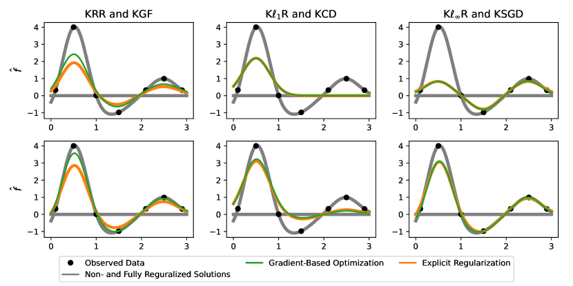
Figure 1: Comparisons of the effects of KRR/KGF, K$\ell_{1}$R/KCD, and K$\ell_{\infty}$R/KSGD on $\bm{\hat{f}}(\bm{x})$. In the top panel, a larger regularization, or a shorter training time, is used than in the bottom panel. For KRR/KGF, we use $t=1/\lambda$, while for the other two cases, $t$ and $\lambda$ are chosen so that the functions coincide as well as possible.
As proposed by Proposition 1, the KGF and KRR solutions differ most where the non-regularized solution is large, and as suggested by Equation 12, the KGF solution lies closer to the observations than the KRR solution does.
For K$\ell_{1}$R/KCD, some observations do not contribute to the solution, resulting in peaks at the more significant observations. For K$\ell_{\infty}$R/KSGD, all observations tend to contribute equally to the solution, resulting in a more robust solution, less sensitive to outliers.
The solutions obtained through early stopping are very similar to those obtained through explicit regularization, although not exactly identical.

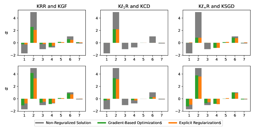
Figure 2: Comparisons of the effects of KRR/KGF, K$\ell_{1}$R/KCD, and K$\ell_{\infty}$R/KSGD on $\bm{\hat{\alpha}}$. In the top panel, a larger regularization, or a shorter training time, is used than in the bottom panel. For KRR/KGF, we use $t=1/\lambda$, while, for the two other cases, $t$ and $\lambda$ are chosen so that the functions coincide as well as possible.
For K$\ell_{1}$R/KCD, some observations do not contribute to the solution, resulting in the corresponding $\hat{\alpha}_{i}$’s being 0. For K$\ell_{\infty}$R/KSGD, all observations tend to contribute equally to the solution, resulting in many $\hat{\alpha}_{i}$’s being equal in magnitude.
The solutions obtained through early stopping are very similar to those obtained through explicit regularization, although not exactly identical.

5.2 Equivalent Interpretations of Kernel Coordinate Descent and Kernel Sign Gradient Descent

As discussed above, using $\ell_{1}$ regularization on $\bm{\alpha}$ promotes a sparse solution, where only the most significant observations are included, while using $\ell_{\infty}$ regularization promotes a solution where all observations contribute equally. Since coordinate descent, and sign gradient descent, with early stopping provide solutions similar to those of $\ell_{1}$ and $\ell_{\infty}$ regularization, the same properties should hold for these algorithms. In Proposition 4, we show that this is the case by using the equivalent interpretation of kernel regression as linear regression in feature space from Equation 4.

Proposition 4.

Solving $\min_{\bm{\alpha}}\left\|\bm{y}-\bm{K}\bm{\alpha}\right\|_{\bm{K}^{-1}}^{2}$ for $\bm{\alpha}$ with

• gradient descent, is equivalent of solving $\min_{\bm{\beta}}\left\|\bm{y}-\bm{\Phi}\bm{\beta}\right\|_{2}^{2}$ for $\bm{\beta}$ with gradient descent.

• coordinate descent, is equivalent of solving $\min_{\bm{\beta}}\left\|\bm{y}-\bm{\Phi}\bm{\beta}\right\|_{\infty}$ for $\bm{\beta}$ with gradient descent.

• sign gradient descent, is equivalent of solving $\min_{\bm{\beta}}\left\|\bm{y}-\bm{\Phi}\bm{\beta}\right\|_{1}$ for $\bm{\beta}$ with gradient descent.

According to Proposition 4, KCD and KSGD correspond to feature space regression with the $\ell_{\infty}$ and $\ell_{1}$ norms, respectively. Note that while we previously discussed different norms for the penalty term, we now consider different norms for the reconstruction term. Regression with the $\ell_{\infty}$ norm minimizes the maximum residual, i.e. more extreme observations contribute more to the solution than less extreme observations do. Vice versa, $\ell_{1}$ norm regression, which is also known as robust regression, is known to be less sensitive to extreme observations than standard, $\ell_{2}$ norm, regression. Thus the takeaways of Proposition 4 are the same as those for explicit regularization. The implications of Proposition 4 can also be observed in Figure 1. For $\ell_{2}$ regression, all residuals are treated equally and all parts of the function are updated at a pace that is proportional to the distance to the solution at convergence. For $\ell_{1}$ regression (KSGD), which is less sensitive to outliers, all parts of the function are initially updated at the same pace, and, in contrast to more moderate observations, the most extreme observations are not fully incorporated until the end of the training. For $\ell_{\infty}$ regression (KCD), which minimizes the maximum residual, the most extreme observations are considered first, while more moderate observations are initially ignored.

6 Experiments

In this section, we demonstrate K$\ell_{1}$R, K$\ell_{\infty}$R, and the corresponding early stopping algorithms, KCD and KSGD, and compare the algorithms to KGD and KRR, on real and synthetic data. We used five different kernels, four Matérn kernels, with different differentiability parameters, $\nu$ (including the Laplace and Gaussian kernels), and the Cauchy kernel. The five different kernels are stated in Table 2.

The evaluation metrics used are

• test $R^{2}$, i.e. the proportion of the variance in test $\bm{y}$ that is explained by the model.

• computation time in seconds.

• model sparsity, calculated as the fraction between included and available observations (only for K$\ell_{1}$R/KCD).

For the explicitly regularized algorithms, the bandwidth and regularization strengths were selected through 10-fold cross-validation with $30\times 30$ logarithmically spaced values. For the early stopping algorithms, 10-fold cross-validation was used for bandwidth selection, with the same 30 candidate bandwidths as for the explicitly regularized models. The stopping times were selected by monitoring performance on validation data. All statistical tests were performed using Wilcoxon signed-rank tests. The experiments were run on a cluster with Intel Xeon Gold 6130, 2.10 GHz processors. For the iterative algorithms, we used an optimization step size of 0.01.

Table 2: Kernels used in the experiments

Name	Equation
Matérn, $\nu=\frac{1}{2}$, (Laplace)	$\exp\left(-\frac{\|\bm{x}-\bm{x^{\prime}}\|_{2}}{\sigma}\right)$
Matérn, $\nu=\frac{3}{2}$,	$\left(1+\frac{\sqrt{3}\cdot\|\bm{x}-\bm{x^{\prime}}\|_{2}}{\sigma}\right)\cdot\exp\left(-\frac{\sqrt{3}\cdot\|\bm{x}-\bm{x^{\prime}}\|_{2}}{\sigma}\right)$
Matérn, $\nu=\frac{5}{2}$,	$\left(1+\frac{\sqrt{5}\cdot\|\bm{x}-\bm{x^{\prime}}\|_{2}}{\sigma}+\frac{5\cdot\|\bm{x}-\bm{x^{\prime}}\|^{2}_{2}}{\sigma}\right)\cdot\exp\left(-\frac{\sqrt{5}\cdot\|\bm{x}-\bm{x^{\prime}}\|_{2}}{\sigma}\right)$
Matérn, $\nu=\infty$, (Gaussian)	$\exp\left(-\frac{\|\bm{x}-\bm{x^{\prime}}\|^{2}_{2}}{2\sigma}\right)$
Cauchy	$\left(1+\frac{\|\bm{x}-\bm{x^{\prime}}\|_{2}^{2}}{\sigma^{2}}\right)^{-1}$

6.1 Synthetic Data

We demonstrate sparse and robust kernel regression on one synthetic data set, respectively. To demonstrate sparse regression on a signal that is mostly zero, with a narrow but distinct peak, 100 observations were sampled according to

$$x\sim\mathcal{U}(-10,10),\ y=e^{-5\cdot x^{2}}+\mathcal{N}(0,0.1^{2}).$$ (16)

For robust regression, to obtain data with outliers, 100 observations were sampled according to

$$x\sim\mathcal{U}(-10,10),\ y=\sin\left(\frac{\pi}{2}\cdot x\right)+\mathcal{C}(0,0.1),$$ (17)

where $\mathcal{C}(0,\gamma)$ is the centered Cauchy distribution with scale parameter $\gamma$. On the first (sparse) data set, we compare KCD, K$\ell_{1}$R, KGD, and KRR, and on the second (robust) data set, we compare KSGD, K$\ell_{\infty}$R, KGD, and KRR.

The results are presented in Tables 3 and 4. For both data sets, using appropriate regularization ($\ell_{1}$ or $\ell_{\infty}$, respectively), either explicitly or through early stopping, outperforms standard KRR/KGD. K$\ell_{1}$R/K$\ell_{\infty}$R and KCD/KSGD perform similarly in terms of $R^{2}$, but the early stopping algorithms are approximately two orders of magnitude faster than the explicitly regularized models. KRR, where a closed-form solution exists, tends to perform faster than the iterative method KGD. Except for computation time, KGD and KRR perform very similarly on the first synthetic data set. However, with outliers present, KGD performs much worse than KRR. This can probably be attributed to the fact that the KGF solution tends to lie closer to the observations than the KRR solution does, as suggested by Equation 12. It is thus more sensitive to outliers.

In Figure 3 we show one realization for each data set. We note that for the first data set, to perform well at the peak, KRR/KGD must also incorporate the noise in the regions where the true signal is zero. K$\ell_{1}$R/KCD include the most significant observations first and are thus able to perform well at the peak while still ignoring the noise in the zero regions. For the second data set, KRR/KGD are more sensitive to the outliers than K$\ell_{\infty}$R/KSGD are, with KGD being more sensitive than KRR.

Table 3: Median and first and third quartile of test $R^{2}$, computation time in seconds, and sparsity for KCD, K$\ell_{1}$R, KGD, and KRR on synthetic data. Occasions when the algorithm performs significantly worse in terms of $R^{2}$/computation time/sparsity than KCD (at significance level 0.01) are marked with bold. In contrast to KRR/KGD, K$\ell_{1}$R/KCD only include a fraction of the observations in the model. KCD is significantly faster than K$\ell_{1}$R.

Kernel	Method	$R^{2}$	Execution Time [s]	Sparsity
$\nu=1/2$ (Laplace)	KCD	$0.89,\ (0.84,0.91)$	$4.81,\ (3.76,5.49)$	$0.14,\ (0.08,0.19)$
	K$\ell_{1}$R	$0.89,\ (0.85,0.91)$	$\bm{159.87,\ (154.78,164.65)}$	$\bm{0.80,\ (0.57,0.95)}$
	KGD	$\bm{0.84,\ (0.79,0.88)}$	$\bm{7.39,\ (2.83,25.29)}$	$\bm{1.00,\ (1.00,1.00)}$
	KRR	$\bm{0.86,\ (0.82,0.88)}$	$3.71,\ (3.68,3.74)$	$\bm{1.00,\ (1.00,1.00)}$
$\nu=3/2$	KCD	$0.91,\ (0.86,0.94)$	$4.05,\ (3.46,4.66)$	$0.07,\ (0.05,0.11)$
	K$\ell_{1}$R	$0.90,\ (0.87,0.93)$	$\bm{161.02,\ (154.70,166.22)}$	$\bm{0.60,\ (0.36,0.82)}$
	KGD	$\bm{0.83,\ (0.76,0.88)}$	$3.60,\ (2.56,10.49)$	$\bm{1.00,\ (1.00,1.00)}$
	KRR	$\bm{0.86,\ (0.83,0.89)}$	$\bm{4.35,\ (4.29,4.38)}$	$\bm{1.00,\ (1.00,1.00)}$
$\nu=5/2$	KCD	$0.92,\ (0.85,0.95)$	$4.03,\ (3.35,4.66)$	$0.07,\ (0.04,0.10)$
	K$\ell_{1}$R	$0.90,\ (0.87,0.93)$	$\bm{162.68,\ (154.70,166.05)}$	$\bm{0.58,\ (0.35,0.78)}$
	KGD	$\bm{0.83,\ (0.77,0.88)}$	$\bm{4.71,\ (2.92,9.24)}$	$\bm{1.00,\ (1.00,1.00)}$
	KRR	$\bm{0.86,\ (0.82,0.89)}$	$\bm{4.70,\ (4.66,4.73)}$	$\bm{1.00,\ (1.00,1.00)}$
$\nu=\infty$ (Gaussian)	KCD	$0.93,\ (0.87,0.96)$	$4.06,\ (3.54,4.69)$	$0.07,\ (0.04,0.09)$
	K$\ell_{1}$R	$0.91,\ (0.88,0.93)$	$\bm{162.73,\ (157.14,167.62)}$	$\bm{0.44,\ (0.33,0.77)}$
	KGD	$\bm{0.80,\ (0.72,0.86)}$	$\bm{13.63,\ (7.45,19.32)}$	$\bm{1.00,\ (1.00,1.00)}$
	KRR	$\bm{0.86,\ (0.81,0.89)}$	$\bm{4.84,\ (4.35,4.99)}$	$\bm{1.00,\ (1.00,1.00)}$
Cauchy	KCD	$0.90,\ (0.82,0.92)$	$3.98,\ (3.27,4.37)$	$0.07,\ (0.04,0.11)$
	K$\ell_{1}$R	$0.89,\ (0.85,0.92)$	$\bm{160.05,\ (153.97,164.57)}$	$\bm{0.65,\ (0.40,0.90)}$
	KGD	$\bm{0.82,\ (0.75,0.86)}$	$3.73,\ (2.47,7.18)$	$\bm{1.00,\ (1.00,1.00)}$
	KRR	$\bm{0.86,\ (0.82,0.89)}$	$3.73,\ (3.57,3.77)$	$\bm{1.00,\ (1.00,1.00)}$

Table 4: Median and first and third quartile of test $R^{2}$ and computation time in seconds for KSGD, K$\ell_{\infty}$R, KGD, and KRR on synthetic data. Occasions when the algorithm performs significantly worse in terms of $R^{2}$/computation time than KSGD (at significance level 0.01) are marked with bold. K$\ell_{\infty}$R/KSGD are less sensitive to outliers than KRR/KGD are, and thus perform better. KSGD is significantly faster than K$\ell_{\infty}$R. KGD is more sensitive to outliers than KRR is.

Kernel	Method	$R^{2}$	Execution Time [s]
$\nu=1/2$ (Laplace)	KSGD	$0.87,\ (0.84,0.91)$	$2.25,\ (1.95,2.49)$
	K$\ell_{\infty}$R	$0.89,\ (0.82,0.93)$	$\bm{736.80,\ (720.44,755.13)}$
	KGD	$\bm{-0.06,\ (-2.06,0.65)}$	$\bm{18.85,\ (6.95,46.37)}$
	KRR	$\bm{0.46,\ (0.11,0.76)}$	$\bm{3.73,\ (3.71,3.76)}$
$\nu=3/2$	KSGD	$0.95,\ (0.91,0.97)$	$3.08,\ (2.78,3.49)$
	K$\ell_{\infty}$R	$\bm{0.92,\ (0.86,0.95)}$	$\bm{725.91,\ (707.37,748.49)}$
	KGD	$\bm{-0.22,\ (-2.62,0.72)}$	$\bm{16.88,\ (7.54,27.15)}$
	KRR	$\bm{0.49,\ (-0.12,0.80)}$	$\bm{4.38,\ (4.35,4.40)}$
$\nu=5/2$	KSGD	$0.95,\ (0.91,0.98)$	$2.85,\ (2.52,3.18)$
	K$\ell_{\infty}$R	$\bm{0.93,\ (0.88,0.95)}$	$\bm{722.53,\ (700.31,749.59)}$
	KGD	$\bm{-0.24,\ (-3.12,0.73)}$	$\bm{20.14,\ (11.25,40.14)}$
	KRR	$\bm{0.49,\ (-0.16,0.81)}$	$\bm{4.71,\ (4.68,4.74)}$
$\nu=\infty$ (Gaussian)	KSGD	$0.96,\ (0.86,0.98)$	$2.43,\ (2.11,2.73)$
	K$\ell_{\infty}$R	$0.94,\ (0.87,0.96)$	$\bm{750.24,\ (730.84,770.17)}$
	KGD	$\bm{-0.34,\ (-3.99,0.76)}$	$\bm{23.80,\ (10.32,33.56)}$
	KRR	$\bm{0.52,\ (-0.11,0.84)}$	$\bm{4.40,\ (4.13,4.46)}$
Cauchy	KSGD	$0.95,\ (0.91,0.97)$	$2.57,\ (2.34,2.76)$
	K$\ell_{\infty}$R	$\bm{0.92,\ (0.85,0.94)}$	$\bm{731.53,\ (711.45,751.03)}$
	KGD	$\bm{-0.29,\ (-2.42,0.72)}$	$\bm{19.43,\ (10.09,32.43)}$
	KRR	$\bm{0.47,\ (-0.14,0.84)}$	$\bm{3.76,\ (3.74,3.79)}$

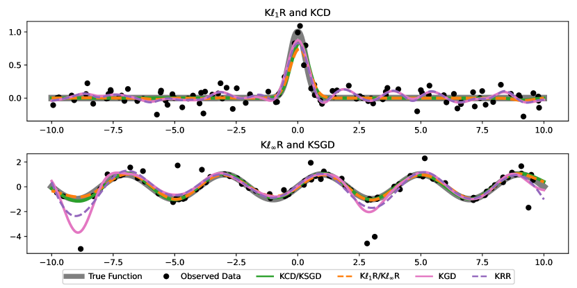
Figure 3: Modelling the data generated by Equations 16 (top) and 17 (bottom) using appropriate regularization and standard KRR/KGD. For the first data set, in contrast to KRR/KGD, K$\ell_{1}$R/KCD are able to model the peak without incorporating the noise. For the second data set, K$\ell_{\infty}$R/KSGD are less affected by the outliers than KRR/KGD are. KGD is more affected by the outliers than KRR is.

6.2 U.K. Temperature Data

We also compared the models on the U.K. temperature data used by Wood et al., (2017). In our experiments, we modeled the daily mean temperature as a function of spatial location for 164 monitoring stations in the U.K. every day during the year 2000. When evaluating robust regression, outliers were introduced by multiplying each element, $y_{i}$, in the response vector by $(1+|\varepsilon_{i}|)$, where $\varepsilon_{i}\sim\mathcal{C}(0,0.01)$ is Cauchy distributed.

The results are presented in Tables 5 and 6. In contrast to KRR/KGD, K$\ell_{1}$R/KCD select models that are sparse in the training data. When outliers are added, K$\ell_{\infty}$R/KSGD perform better than KRR/KGD in terms of $R^{2}$. KCD/KSGD perform significantly faster than K$\ell_{1}$R/K$\ell_{\infty}$R. Again, KGD is more affected by the outliers than KRR is.

Table 5: Median and first and third quartile of test $R^{2}$, computation time in seconds, and sparsity for KCD, K$\ell_{1}$R, KGD, and KRR on the U.K. temperature data over the 366 days. Occasions when the algorithm performs significantly worse in terms of $R^{2}$/computation time/sparsity than KCD (at significance level 0.01) are marked with bold. In contrast to KRR/KGD, K$\ell_{1}$R/KCD only include a fraction of the observations into the model. KCD is significantly faster than K$\ell_{1}$R.

Kernel	Method	$R^{2}$	Execution Time [s]	Sparsity
$\nu=1/2$ (Laplace)	KCD	$0.70,\ (0.46,0.83)$	$44.68,\ (31.26,57.83)$	$0.40,\ (0.29,0.52)$
	K$\ell_{1}$R	$\bm{0.45,\ (0.17,0.67)}$	$\bm{87.79,\ (71.28,103.97)}$	$0.19,\ (0.15,0.25)$
	KGD	$0.76,\ (0.51,0.89)$	$\bm{66.25,\ (46.47,91.29)}$	$\bm{1.00,\ (1.00,1.00)}$
	KRR	$0.75,\ (0.52,0.88)$	$4.72,\ (4.45,5.00)$	$\bm{1.00,\ (1.00,1.00)}$
$\nu=3/2$	KCD	$0.63,\ (0.39,0.79)$	$34.45,\ (24.88,47.12)$	$0.22,\ (0.15,0.33)$
	K$\ell_{1}$R	$\bm{0.47,\ (0.18,0.69)}$	$\bm{88.38,\ (72.85,106.20)}$	$0.18,\ (0.15,0.23)$
	KGD	$0.70,\ (0.44,0.85)$	$\bm{70.60,\ (54.46,89.79)}$	$\bm{1.00,\ (1.00,1.00)}$
	KRR	$0.71,\ (0.49,0.85)$	$5.64,\ (5.23,5.92)$	$\bm{1.00,\ (1.00,1.00)}$
$\nu=5/2$	KCD	$0.60,\ (0.37,0.78)$	$31.52,\ (22.42,44.85)$	$0.19,\ (0.13,0.30)$
	K$\ell_{1}$R	$\bm{0.47,\ (0.18,0.69)}$	$\bm{89.81,\ (73.20,105.86)}$	$0.18,\ (0.15,0.23)$
	KGD	$0.69,\ (0.40,0.84)$	$\bm{71.08,\ (55.91,89.46)}$	$\bm{1.00,\ (1.00,1.00)}$
	KRR	$0.69,\ (0.46,0.84)$	$6.22,\ (5.83,6.58)$	$\bm{1.00,\ (1.00,1.00)}$
$\nu=\infty$ (Gaussian)	KCD	$0.55,\ (0.32,0.75)$	$25.72,\ (18.12,37.35)$	$0.17,\ (0.10,0.26)$
	K$\ell_{1}$R	$\bm{0.48,\ (0.20,0.69)}$	$\bm{88.04,\ (72.97,104.45)}$	$0.18,\ (0.15,0.23)$
	KGD	$0.64,\ (0.36,0.82)$	$\bm{77.90,\ (59.44,94.69)}$	$\bm{1.00,\ (1.00,1.00)}$
	KRR	$0.67,\ (0.41,0.82)$	$5.65,\ (5.33,6.13)$	$\bm{1.00,\ (1.00,1.00)}$
Cauchy	KCD	$0.64,\ (0.40,0.79)$	$38.04,\ (27.31,51.77)$	$0.23,\ (0.15,0.39)$
	K$\ell_{1}$R	$\bm{0.46,\ (0.18,0.69)}$	$\bm{87.78,\ (71.43,106.03)}$	$0.18,\ (0.15,0.24)$
	KGD	$0.68,\ (0.42,0.84)$	$\bm{68.20,\ (52.66,84.48)}$	$\bm{1.00,\ (1.00,1.00)}$
	KRR	$0.70,\ (0.48,0.85)$	$4.72,\ (4.43,5.00)$	$\bm{1.00,\ (1.00,1.00)}$

Table 6: Median and first and third quartile of test $R^{2}$ and computation time in seconds for KSGD, K$\ell_{\infty}$R, KGD, and KRR on the outlier injected U.K. temperature data over the 366 days. Occasions when the algorithm performs significantly worse in terms of $R^{2}$/computation time than KSGD (at significance level 0.01) are marked with bold. K$\ell_{\infty}$R/KSGD are less affected by the outliers than KRR/KGD are and thus perform better. KSGD is significantly faster than K$\ell_{\infty}$R. KGD is more sensitive to outliers than KRR is.

Kernel	Method	$R^{2}$	Execution Time [s]
$\nu=1/2$ (Laplace)	KSGD	$0.58,\ (0.25,0.76)$	$3.35,\ (2.88,4.46)$
	K$\ell_{\infty}$R	$0.61,\ (0.35,0.79)$	$\bm{805.13,\ (734.67,905.81)}$
	KGD	$0.48,\ (-0.40,0.78)$	$\bm{47.03,\ (18.56,80.58)}$
	KRR	$0.46,\ (-0.01,0.77)$	$\bm{4.77,\ (4.46,5.07)}$
$\nu=3/2$	KSGD	$0.60,\ (0.31,0.80)$	$3.83,\ (3.21,5.15)$
	K$\ell_{\infty}$R	$0.61,\ (0.31,0.78)$	$\bm{806.83,\ (732.84,909.09)}$
	KGD	$\bm{0.38,\ (-0.84,0.74)}$	$\bm{51.49,\ (26.32,74.58)}$
	KRR	$\bm{0.42,\ (0.02,0.73)}$	$\bm{5.58,\ (5.26,5.91)}$
$\nu=5/2$	KSGD	$0.57,\ (0.29,0.78)$	$3.91,\ (3.20,5.25)$
	K$\ell_{\infty}$R	$0.60,\ (0.28,0.77)$	$\bm{808.60,\ (740.00,919.48)}$
	KGD	$\bm{0.34,\ (-1.07,0.72)}$	$\bm{53.40,\ (26.99,76.82)}$
	KRR	$\bm{0.40,\ (-0.02,0.73)}$	$\bm{6.19,\ (5.84,6.55)}$
$\nu=\infty$ (Gaussian)	KSGD	$0.56,\ (0.24,0.77)$	$3.89,\ (3.28,4.98)$
	K$\ell_{\infty}$R	$0.58,\ (0.28,0.76)$	$\bm{824.79,\ (753.40,933.57)}$
	KGD	$\bm{0.24,\ (-1.34,0.70)}$	$\bm{58.28,\ (34.78,80.10)}$
	KRR	$\bm{0.38,\ (-0.02,0.72)}$	$\bm{5.72,\ (5.34,6.11)}$
Cauchy	KSGD	$0.59,\ (0.29,0.80)$	$3.88,\ (3.18,5.10)$
	K$\ell_{\infty}$R	$0.61,\ (0.31,0.77)$	$\bm{803.72,\ (734.21,908.72)}$
	KGD	$\bm{0.33,\ (-1.30,0.72)}$	$\bm{49.85,\ (27.28,73.81)}$
	KRR	$\bm{0.41,\ (0.00,0.73)}$	$\bm{4.68,\ (4.41,4.95)}$

7 Conclusions

We introduced an equivalent formulation of kernel ridge regression and used it to define kernel regression with the $\ell_{1}$ and $\ell_{\infty}$ penalties, and for solving kernel regression with gradient-based optimization methods. We introduced the methods kernel coordinate descent and kernel sign gradient descent, and utilized the similarities between $\ell_{1}$ regularization and coordinate descent (forward stagewise regression), and between $\ell_{\infty}$ regularization and sign gradient descent, to obtain computationally efficient algorithms for sparse and robust kernel regression, respectively. We theoretically analyzed the similarities between kernel gradient descent, kernel coordinate descent, and kernel sign gradient descent and the corresponding explicitly regularized kernel regression methods, and compared the methods on real and synthetic data.

Our generalizations of kernel ridge regression, together with regularization through early stopping, enable computationally efficient, kernelized sparse, and robust, regression. Although we investigated only kernel regression with the $\ell_{2}$, $\ell_{1}$, and $\ell_{\infty}$ penalties, many other penalties could be considered, such as the adaptive lasso (Zou,, 2006), the group lasso (Yuan and Lin,, 2006), the exclusive lasso (Zhou et al.,, 2010) and OSCAR (Bondell and Reich,, 2008). This is, however, left for future work.

Code is available at https://github.com/allerbo/gradient_based_kernel_regression.

Appendix A Calculations for $[\bm{\hat{f}}^{\top},\bm{\hat{f}^{*}}{{}^{\top}}]^{\top}$

In this section, we revisit some of the calculations in the main manuscript and reformulate them directly in terms of $[\bm{\hat{f}}^{\top},\bm{\hat{f}^{*}}{{}^{\top}}]^{\top}$, rather than obtaining them by multiplying $\bm{\alpha}$ by $[\bm{K}^{\top},\bm{K^{*}}{{}^{\top}}]^{\top}$.

A.1 Equivalent Formulations of Kernel Ridge Regression

In Lemma 4, we present three different objective functions, that all render the same solution for $[\bm{\hat{f}}^{\top},\bm{\hat{f}^{*}}{{}^{\top}}]^{\top}$ as in Equation 3. When expressing KRR in terms of $\bm{\alpha}\in\mathbb{R}^{n}$, it is enough to include $\bm{K}\in\mathbb{R}^{n\times n}$ in the expression to capture the dynamics of the kernel. However, when expressing KRR in terms of $[\bm{\hat{f}}^{\top},\bm{\hat{f}^{*}}{{}^{\top}}]^{\top}\in\mathbb{R}^{n+n^{*}}$, we need to introduce the larger kernel matrix

$$\bm{K^{**}}:=\begin{bmatrix}\bm{K}(\bm{X},\bm{X})&\bm{K}(\bm{X},\bm{X^{*}})\\ \bm{K}(\bm{X^{*}},\bm{X})&\bm{K}(\bm{X^{*}},\bm{X^{*}})\end{bmatrix}\in\mathbb{R}^{(n+n^{*})\times(n+n^{*})}$$

in order to let the kernel affect not only $\bm{f}\in\mathbb{R}^{n}$, but also $\bm{f^{*}}\in\mathbb{R}^{n^{*}}$. Furthermore, we need the extended response vector $[\bm{y}^{\top},\bm{\tilde{y}}^{\top}]^{\top}$, where $\bm{\tilde{y}}$ is a copy of $\bm{f^{*}}$, so that $\bm{\tilde{y}}-\bm{f^{*}}=\bm{0}$.

Lemma 4.

$$\begin{bmatrix}\bm{\hat{f}}\\ \bm{\hat{f}^{*}}\end{bmatrix}= \operatorname*{arg\,min}_{[\bm{f}^{\top},\bm{f^{*}}{{}^{\top}}]^{\top}\in\mathbb{R}^{n+n^{*}}}\frac{1}{2}\left\|\bm{y}-\bm{f}\right\|_{2}^{2}+\frac{\lambda}{2}\left\|\begin{bmatrix}\bm{f}\\ \bm{f^{*}}\end{bmatrix}\right\|^{2}_{(\bm{K^{**}})^{-1}}$$ (18a)

$$= \operatorname*{arg\,min}_{[\bm{f}^{\top},\bm{f^{*}}{{}^{\top}}]^{\top}\in\mathbb{R}^{n+n^{*}}}\frac{1}{2}\left\|\begin{bmatrix}\bm{y}\\ \bm{\tilde{y}}\end{bmatrix}-\begin{bmatrix}\bm{f}\\ \bm{f^{*}}\end{bmatrix}\right\|_{2}^{2}+\frac{\lambda}{2}\left\|\begin{bmatrix}\bm{f}\\ \bm{f^{*}}\end{bmatrix}\right\|^{2}_{(\bm{K^{**}})^{-1}}$$ (18b)

$$= \operatorname*{arg\,min}_{[\bm{f}^{\top},\bm{f^{*}}{{}^{\top}}]^{\top}\in\mathbb{R}^{n+n^{*}}}\frac{1}{2}\left\|\begin{bmatrix}\bm{y}\\ \bm{\tilde{y}}\end{bmatrix}-\begin{bmatrix}\bm{f}\\ \bm{f^{*}}\end{bmatrix}\right\|_{\bm{K^{**}}}^{2}+\frac{\lambda}{2}\left\|\begin{bmatrix}\bm{f}\\ \bm{f^{*}}\end{bmatrix}\right\|^{2}_{2}$$ (18c)

$$= \begin{bmatrix}\bm{K}\\ \bm{K^{*}}\end{bmatrix}\left(\bm{K}+\lambda\bm{I}\right)^{-1}\bm{y}.$$

Remark 1: We assert that $\bm{f^{*}}$ does not affect the reconstruction error by requiring that $\bm{\tilde{y}}-\bm{f^{*}}=\bm{0}$, We may, however, not define $\bm{\tilde{y}}$ to equal $\bm{f^{*}}$, since we do not want $\bm{\tilde{y}}$ to be considered when differentiating Equations 18b and 18c with respect to $\bm{f^{*}}$.
Remark 2: The term $\left\|\begin{bmatrix}\bm{f}\\ \bm{f^{*}}\end{bmatrix}\right\|^{2}_{(\bm{K^{**}})^{-1}}$, might appear a bit peculiar, including the inverse of the extended kernel matrix. However, it is very closely related to the expression for the reproducing kernel Hilbert space norm, $\|f\|^{2}_{\mathcal{H}_{k}}$, obtained when expressing the functions $f$ and $k$ in terms of the orthogonal basis given by Mercer’s Theorem: $f(\bm{x})=\sum_{i=1}^{\infty}f_{i}\phi_{i}(\bm{x})$ and $k(\bm{x},\bm{x^{\prime}})=\sum_{i=1}^{\infty}k_{i}\phi_{i}(\bm{x})\phi_{i}(\bm{x^{\prime}})$, with $\|f\|^{2}_{\mathcal{H}_{k}}:=\sum_{i=1}^{\infty}\frac{f_{i}^{2}}{k_{i}}$. Defining the vector $\bm{\tilde{f}}$ and the diagonal matrix $\bm{\tilde{K}}$ according to $\bm{\tilde{f}}_{i}=f_{i}$ and $\bm{\tilde{K}}_{ii}=k_{i}$, we obtain $\|f\|^{2}_{\mathcal{H}_{k}}=\sum_{i=1}^{\infty}\frac{f_{i}^{2}}{k_{i}}=\bm{\tilde{f}}^{\top}\bm{\tilde{K}}^{-1}\bm{\tilde{f}}=\|\bm{\tilde{f}}\|_{\bm{\tilde{K}}^{-1}}^{2}$.

A.2 Kernel Gradient Descent and Kernel Gradient Flow

The gradient of Equation 18c with respect to $[\bm{f}^{\top},\bm{f^{*}}{{}^{\top}}]^{\top}$ is

$$\begin{bmatrix}\bm{K}\\ \bm{K^{*}}\end{bmatrix}(\bm{f}-\bm{y})+\lambda\begin{bmatrix}\bm{f}\\ \bm{f^{*}}\end{bmatrix},$$

which coincides with Equation 7, as expected. Thus, the KGD update in $[\bm{\hat{f}}^{\top},\bm{\hat{f}^{*}}{{}^{\top}}]^{\top}$ is

$$\begin{bmatrix}\bm{\hat{f}}_{k+1}\\ \bm{\hat{f}^{*}}_{k+1}\end{bmatrix}=\begin{bmatrix}\bm{\hat{f}}_{k}\\ \bm{\hat{f}^{*}}_{k}\end{bmatrix}+\eta\cdot\begin{bmatrix}\bm{K}\\ \bm{K^{*}}\end{bmatrix}\left(\bm{y}-\bm{\hat{f}}_{k}\right),\ \begin{bmatrix}\bm{\hat{f}}_{0}\\ \bm{\hat{f}^{*}}_{0}\end{bmatrix}=\bm{0},$$

with the corresponding differential equation

$$\frac{\partial}{\partial t}\left(\begin{bmatrix}\bm{\hat{f}}(t)\\ \bm{\hat{f}^{*}}(t)\end{bmatrix}\right)=\begin{bmatrix}\bm{K}\\ \bm{K^{*}}\end{bmatrix}\left(\bm{y}-\bm{\hat{f}}(t)\right),\ \begin{bmatrix}\bm{\hat{f}}(0)\\ \bm{\hat{f}^{*}}(0)\end{bmatrix}=\bm{0},$$ (19)

whose solution is stated in Lemma 5

Lemma 5.

The solution to the differential equation in Equation 19 is

$$\begin{bmatrix}\bm{\hat{f}}(t)\\ \bm{\hat{f}^{*}}(t)\end{bmatrix}=\begin{bmatrix}\bm{I}\\ \bm{K^{*}}\bm{K}^{-1}\end{bmatrix}(\bm{I}-\exp(-t\bm{K}))\bm{y}$$

A.3 Kernel Regression with the $\ell_{1}$ and $\ell_{\infty}$ Norms

If we replace the squared $\ell_{2}$ norm in Equation 18c by the $\ell_{1}$ and $\ell_{\infty}$ norms, we obtain

$$\operatorname*{arg\,min}_{[\bm{f}^{\top},\bm{f^{*}}{{}^{\top}}]^{\top}\in\mathbb{R}^{n+n^{*}}}\frac{1}{2}\left\|\begin{bmatrix}\bm{y}\\ \bm{\tilde{y}}\end{bmatrix}-\begin{bmatrix}\bm{f}\\ \bm{f^{*}}\end{bmatrix}\right\|_{\bm{K^{**}}}^{2}+\lambda\left\|\begin{bmatrix}\bm{f}\\ \bm{f^{*}}\end{bmatrix}\right\|_{1}$$ (20)

and

$$\operatorname*{arg\,min}_{[\bm{f}^{\top},\bm{f^{*}}{{}^{\top}}]^{\top}\in\mathbb{R}^{n+n^{*}}}\frac{1}{2}\left\|\begin{bmatrix}\bm{y}\\ \bm{\tilde{y}}\end{bmatrix}-\begin{bmatrix}\bm{f}\\ \bm{f^{*}}\end{bmatrix}\right\|_{\bm{K^{**}}}^{2}+\lambda\left\|\begin{bmatrix}\bm{f}\\ \bm{f^{*}}\end{bmatrix}\right\|_{\infty}.$$ (21)

In contrast to ridge regression, where the formulations in $\bm{\alpha}$ and $[\bm{f}^{\top},\bm{f^{*}}{{}^{\top}}]^{\top}$ are equivalent in the sense that the latter can always be obtained from the first through multiplication with $[\bm{K}^{\top},\bm{K^{*}}{{}^{\top}}]^{\top}$, the solutions of Equations 20 and 21 cannot be obtained from the solutions of Equations 13 and 14.

Since $\ell_{1}$ regularization promotes a sparse solution, with the most significant parameters included first, in the solutions of Equation 20, many of the predictions equal exactly zero, with only the most extreme predictions being non-zero. For $\ell_{\infty}$ regularization, which promotes a solution where the parameters have equal absolute values, many of the predictions in the solution to Equation 21 are exactly equal. In Figure 4, we exemplify this for explicit regularization for two different regularization strengths. Even though it is technically possible to use gradient-based optimization with early stopping for $[\bm{f}^{\top},\bm{f^{*}}{{}^{\top}}]^{\top}$, since the reconstruction error, and thus the gradient, is affected only by $\bm{f}$ and not by $\bm{f^{*}}$, this does not work well the for coordinate and sign gradient descent algorithms.

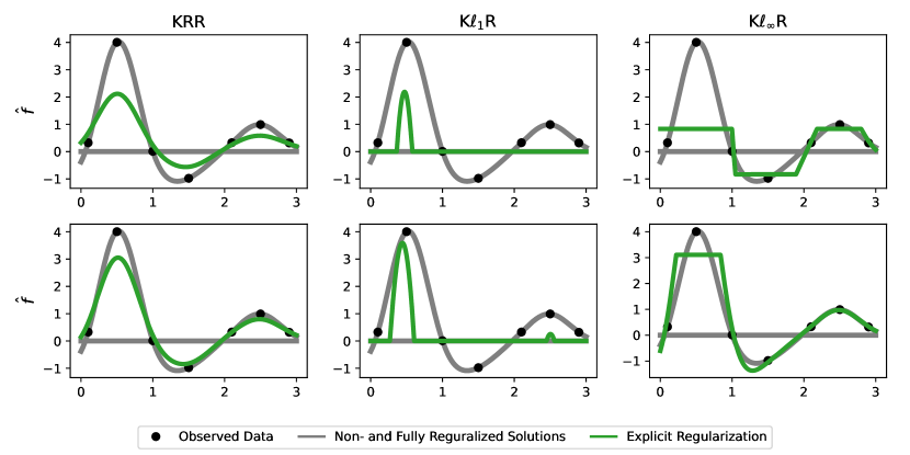
Figure 4: Comparisons of the effects of $\ell_{2}$, $\ell_{1}$, and $\ell_{\infty}$ regularization on $[\bm{f}^{\top},\bm{f^{*}}{{}^{\top}}]^{\top}$.
In the top panel, a larger regularization, or a shorter training time, is used than in the bottom panel.
For $\ell_{1}$ regularization, many predictions are set exactly to zero, with peaks at some extreme predictions. For $\ell_{\infty}$ regularization, the absolute values of many predictions exactly equal. To obtain this, compared to the non-regularized solution, some predictions are shifted away from zero, while some predictions are shifted toward zero.

Finally, in Proposition 5, we present the analogue of Proposition 3 for $[\bm{f}^{\top},\bm{f^{*}}{{}^{\top}}]^{\top}$.

Proposition 5.

For $\bm{f^{{}^{+}}}:=[\bm{f}^{\top},\bm{f^{*}}{{}^{\top}}]^{\top}$ and $\bm{y^{{}^{+}}}:=[\bm{y}^{\top},\bm{\tilde{y}}^{\top}]^{\top}$, where $\bm{\tilde{y}}-\bm{f^{*}}=\bm{0}$, let $\bm{\hat{f}}^{\bm{+}\infty}(c)$ denote the solution to

$$\min_{\bm{f^{{}^{+}}}\in\mathbb{R}^{n+n^{*}}}\left\|\bm{y^{{}^{+}}}-\bm{f^{{}^{+}}}\right\|_{\bm{K^{**}}}^{2}\text{ s.t. }\|\bm{f^{{}^{+}}}\|_{\infty}\leq c,$$

and let $\bm{\hat{f}}^{\bm{+}\text{SGF}}(t)$ denote the solution to

$$\frac{\partial\bm{f^{{}^{+}}}(t)}{\partial t}=\text{sign}\left(-\frac{\partial}{\partial\bm{f^{{}^{+}}}(t)}\left(\left\|\bm{y^{{}^{+}}}-\bm{f^{{}^{+}}}(t)\right\|_{\bm{K^{**}}}^{2}\right)\right),\ \bm{f^{{}^{+}}}(0)=\bm{0}.$$

When $\bm{K^{**}}$ is diagonal, with elements $\{k_{ii}\}_{i=1}^{n+n^{*}}$, $k_{ii}>0$, the two solutions decompose element-wise and coincide for $c=t$:

$$\hat{f}^{+\infty}_{i}(t)=\hat{f}^{+\text{SGF}}_{i}(t)=\begin{cases}\text{sign}(y_{i})\cdot\min(t,|y_{i}|)&\text{if }i\leq n\\ 0&\text{if }i>n.\end{cases}$$

Appendix B Proofs

Proof of Lemma 1.

Differentiating Equation 5b with respect to $\bm{\alpha}$ and setting the gradient to $\bm{0}$, we obtain

$$\bm{0}=\frac{\partial}{\partial\bm{\hat{\alpha}}}\left(\frac{1}{2}\left\|\bm{y}-\bm{K}\bm{\hat{\alpha}}\right\|_{\bm{K}^{-1}}^{2}+\frac{\lambda}{2}\|\bm{\hat{\alpha}}\|^{2}_{2}\right)=-\bm{y}+\bm{K}\bm{\hat{\alpha}}+\lambda\bm{\hat{\alpha}}=-\bm{y}+(\bm{K}+\lambda\bm{I})\bm{\hat{\alpha}}\iff\bm{\hat{\alpha}}=(\bm{K}+\lambda\bm{I})^{-1}\bm{y}.$$

∎

Proof of Lemma 2.

With $\bm{\hat{\eta}}(t)=\bm{K}\bm{\hat{\alpha}}(t)-\bm{y}$, we obtain $\frac{d\bm{\hat{\eta}}(t)}{dt}=\bm{K}\frac{d\bm{\hat{\alpha}}(t)}{dt}$ and Equation 9 can be written as

$$\frac{d\bm{\hat{\eta}}(t)}{dt}=-\bm{K}\bm{\hat{\eta}}(t)\iff\bm{\hat{\eta}}(t)=\exp\left(-t\bm{K}\right)\bm{\hat{\eta}_{0}}.$$

Now,

$$\bm{\hat{\alpha}}(0)=\bm{0}\implies\bm{\hat{\eta}_{0}}=\bm{\hat{\eta}}(0)=-\bm{y}\implies\bm{\hat{\eta}}(t)=-\exp(-t\bm{K})\bm{y}.$$

Solving for $\bm{\hat{\alpha}}(t)$, we obtain

$$\bm{\hat{\alpha}}(t)=\bm{K}^{-1}\left(\bm{I}-\exp(-t\bm{K})\right)\bm{y}=\left(\bm{I}-\exp(-t\bm{K})\right)\bm{K}^{-1}\bm{y}.$$

∎

Proof of Remark 3 of Lemma 2.

The differential equation in Equation 9 can be obtained by writing

$$\bm{\hat{\alpha}}_{k+1}=\bm{\hat{\alpha}}_{k}+\eta\cdot\left(\bm{y}-\bm{K}\bm{\hat{\alpha}}_{k}\right)$$

as

$$\bm{\hat{\alpha}}(t+\Delta t)=\bm{\hat{\alpha}}(t)+\Delta t\cdot\left(\bm{y}-\bm{K}\bm{\hat{\alpha}}(t)\right),$$

rearranging and letting $\Delta t\to 0$, to obtain

$$\frac{d\bm{\hat{\alpha}}(t)}{dt}=\lim_{\Delta t\to 0}\left(\frac{\bm{\hat{\alpha}}(t+\Delta t)-\bm{\hat{\alpha}}(t)}{\Delta t}\right)=\bm{y}-\bm{K}\bm{\hat{\alpha}}(t).$$

For momentum and Nesterov accelerated gradient, the update rule for $\bm{\hat{\alpha}}$ in Equation 8 generalizes to

$$\bm{\hat{\alpha}}(t+\Delta t)=\bm{\hat{\alpha}}(t)+\gamma\cdot\left(\bm{\hat{\alpha}}(t)-\bm{\hat{\alpha}}(t-\Delta t)\right)+\Delta t\cdot\left(\bm{y}-\bm{K}\left(\bm{\hat{\alpha}}(t)+\mathbb{I}_{\text{NAG}}\cdot\gamma\cdot\left(\bm{\hat{\alpha}}(t)-\bm{\hat{\alpha}}(t-\Delta t)\right)\right)\right),$$

where $\gamma\in[0,1)$ is the strength of the momentum and $\mathbb{I}_{\text{NAG}}\in\{0,1\}$ decides whether to use Nesterov accelerated gradient or not. Rearranging, we obtain

$$\frac{\bm{\hat{\alpha}}(t+\Delta t)-\bm{\hat{\alpha}}(t)}{\Delta t}-\gamma\cdot\frac{\bm{\hat{\alpha}}(t)-\bm{\hat{\alpha}}(t-\Delta t)}{\Delta t}=\bm{y}-\bm{K}\left(\bm{\hat{\alpha}}(t)+\mathbb{I}_{\text{NAG}}\cdot\gamma\cdot\left(\bm{\hat{\alpha}}(t)-\bm{\hat{\alpha}}(t-\Delta t)\right)\right),$$

and, when $\Delta t\to 0$,

$$(1-\gamma)\cdot\frac{d\bm{\hat{\alpha}}(t)}{dt}=\bm{y}-\bm{K}\bm{\hat{\alpha}}(t).$$

Solving the differential equations in the same way as in Lemma 2, we obtain

$$\bm{\hat{\alpha}}(t)=\left(\bm{I}-\exp\left(-\frac{t}{1-\gamma}\bm{K}\right)\right)\bm{K}^{-1}\bm{y}.$$

∎

Proof of Lemma 3.

$$\left(\bm{K}+\lambda\bm{I}\right)^{-1} =\left(\bm{K}+\lambda\bm{I}\right)^{-1}\underbrace{(\bm{K}+\lambda\bm{I}-\lambda\bm{I})\bm{K}^{-1}}_{=\bm{I}}=\left(\bm{I}-\lambda\left(\bm{K}+\lambda\bm{I}\right)^{-1}\right)\bm{K}^{-1}$$

$$=\left(\bm{I}-\left(\bm{I}+1/\lambda\cdot\bm{K}\right)^{-1}\right)\bm{K}^{-1}.$$

∎

Proof of Proposition 1.

By using the fact that $\bm{K}$, $\bm{K}^{-1}$ and $\bm{\Delta_{K}}:=\left(\left(\bm{I}+t\bm{K}\right)^{-1}-\exp(-t\bm{K})\right)$ commute, we obtain

$$\bm{\hat{\alpha}}_{\text{KGF}}(t)-\bm{\hat{\alpha}}_{\text{KRR}}(1/t) =\left(\bm{I}-\exp(-t\bm{K})\right)\bm{K}^{-1}\bm{y}-\left(\bm{I}-\left(\bm{I}+t\bm{K}\right)^{-1}\right)\bm{K}^{-1}\bm{y}$$

$$=\underbrace{\left(\left(\bm{I}+t\bm{K}\right)^{-1}-\exp(-t\bm{K})\right)}_{=:\bm{\Delta_{K}}}\bm{K}^{-1}\bm{y}=\bm{\Delta_{K}}\bm{K}^{-1}\bm{y},$$

$$\bm{\hat{f}}_{\text{KGF}}(\bm{X},t)-\bm{\hat{f}}_{\text{KRR}}(\bm{X},1/t) =\bm{K}\left(\bm{\hat{\alpha}}_{\text{KGF}}-\bm{\hat{\alpha}}_{\text{KRR}}\right)=\bm{K}\bm{\Delta_{K}}\bm{K}^{-1}\bm{y}=\bm{\Delta_{K}}\bm{K}\bm{K}^{-1}\bm{y}=\bm{\Delta_{K}}\bm{y},$$

$$\hat{f}_{\text{KGF}}(\bm{x^{*}},t)-\hat{f}_{\text{KRR}}(\bm{x^{*}},1/t) =\bm{k}(\bm{x^{*}})^{\top}\left(\bm{\hat{\alpha}}_{\text{KGF}}-\bm{\hat{\alpha}}_{\text{KRR}}\right)=\bm{k}(\bm{x^{*}})^{\top}\bm{\Delta_{K}}\bm{K}^{-1}\bm{y}=\bm{k}(\bm{x^{*}})^{\top}\bm{K}^{-1}\bm{\Delta_{K}}\bm{y},$$

We denote the singular value decomposition of the symmetric matrix $\bm{K}$ by $\bm{K}=\bm{U}\bm{S}\bm{U}^{\top}$, where $\bm{S}$ is a diagonal matrix with diagonal elements $\bm{S}_{ii}=s_{i}$. Then $\bm{\Delta_{K}}=\bm{U}\bm{D}\bm{U}^{\top}$, where $\bm{D}$ is a diagonal matrix with entries

$$\bm{D}_{ii}=d_{i}=\frac{1}{1+t\cdot s_{i}}-e^{t\cdot s_{i}}.$$

Since for any vector $\bm{x}$ and any diagonal matrix $\bm{D}$,

$$\bm{x}^{\top}\bm{D}\bm{x}=\sum_{i}x_{i}^{2}\cdot d_{i}\leq\sum_{i}x_{i}^{2}\cdot\max_{i}d_{i}=\bm{x}^{\top}\bm{x}\cdot\max_{i}d_{i},$$ (22)

and since $\bm{K}^{-1}$ and $\bm{\Delta_{K}}$ are both symmetric,

$$\|\bm{\hat{\alpha}}_{\text{KGF}}(t)-\bm{\hat{\alpha}}_{\text{KRR}}(1/t)\|_{2}^{2} =\bm{y}^{\top}\bm{K}^{-1}\bm{\Delta_{K}}\bm{\Delta_{K}}\bm{K}^{-1}\bm{y}=\bm{y}^{\top}\bm{K}^{-1}\bm{U}\bm{D}^{2}\bm{U}^{\top}\bm{K}^{-1}\bm{y}$$

$$\leq\bm{y}^{\top}\bm{K}^{-1}\underbrace{\bm{U}\bm{U}^{\top}}_{=\bm{I}}\bm{K}^{-1}\bm{y}\cdot\max_{i}d_{i}^{2}=\|\bm{K}^{-1}\bm{y}\|_{2}^{2}\cdot\max_{i}d_{i}^{2},$$

and

$$\|\bm{\hat{f}}_{\text{KGF}}(\bm{X},t)-\bm{\hat{f}}_{\text{KRR}}(\bm{X},1/t)\|_{2}^{2}=\bm{y}^{\top}\bm{\Delta_{K}}\bm{\Delta_{K}}\bm{y}=\bm{y}^{\top}\bm{U}\bm{D}^{2}\bm{U}^{\top}\bm{y}\leq\bm{y}^{\top}\underbrace{\bm{U}\bm{U}^{\top}}_{=\bm{I}}\bm{y}\cdot\max_{i}d_{i}^{2}=\|\bm{y}\|_{2}^{2}\cdot\max_{i}d_{i}^{2}.$$

For out-of-sample predictions, calculations become different, since $\bm{k}(\bm{x^{*}})$ and $\bm{K}$ do not commute. Hence we need to take expectation over $\bm{y}$. We first note that for $\bm{y}=\bm{K}\bm{\alpha_{0}}+\bm{\varepsilon}$, where $\bm{\alpha_{0}}\sim(\bm{0},\bm{\Sigma_{\alpha}})$, and $\bm{\varepsilon}\sim(\bm{0},\sigma_{\varepsilon}^{2}\bm{I})$, and where $\bm{K}$ and $\bm{\Sigma_{\alpha}}$ commute,

$$\mathbb{E}_{\bm{\varepsilon},\bm{\alpha_{0}}}\left(\bm{y}\bm{y}^{\top}\right)=\bm{K}\mathbb{E}\left(\bm{\alpha_{0}}\bm{\alpha_{0}}^{\top}\right)\bm{K}+2\bm{K}\mathbb{E}(\bm{\alpha_{0}})\mathbb{E}(\bm{\varepsilon})^{\top}+\mathbb{E}(\bm{\varepsilon}\bm{\varepsilon}^{\top})=\bm{\Sigma_{\alpha}}\bm{K}^{2}+\sigma_{\varepsilon}^{2}\bm{I}.$$

Now,

$$\mathbb{E}_{\bm{\varepsilon},\bm{\alpha_{0}}}\left(\left(\hat{f}_{\text{KGF}}(\bm{x^{*}},t)-\hat{f}_{\text{KRR}}(\bm{x^{*}},1/t)\right)^{2}\right)=\mathbb{E}_{\bm{\varepsilon},\bm{\alpha_{0}}}\left(\bm{k}(\bm{x^{*}})^{\top}\bm{K}^{-1}\bm{\Delta_{K}}\bm{y}\bm{y}^{\top}\bm{\Delta_{K}}\bm{K}^{-1}\bm{k}(\bm{x^{*}})\right)$$

$$=\bm{k}(\bm{x^{*}})^{\top}\bm{K}^{-1}\bm{\Delta_{K}}\left(\bm{\Sigma_{\alpha}}\bm{K}^{2}+\sigma_{\varepsilon}^{2}\bm{I}\right)\bm{\Delta_{K}}\bm{K}^{-1}\bm{k}(\bm{x^{*}})$$

$$=\bm{k}(\bm{x^{*}})^{\top}\bm{K}^{-1}\bm{\Sigma_{\alpha}}^{1/2}\bm{K}\bm{U}\bm{D}^{2}\bm{U}^{\top}\bm{K}\bm{\Sigma_{\alpha}}^{1/2}\bm{K}^{-1}\bm{k}(\bm{x^{*}})+\sigma_{\varepsilon}^{2}\cdot\bm{k}(\bm{x^{*}})^{\top}\bm{K}^{-1}\bm{U}\bm{D}^{2}\bm{U}^{\top}\bm{K}^{-1}\bm{k}(\bm{x^{*}})$$

$$\leq\left(\bm{k}(\bm{x^{*}})^{\top}\bm{K}^{-1}\bm{\Sigma_{\alpha}}^{1/2}\bm{K}\underbrace{\bm{U}\bm{U}^{\top}}_{=\bm{I}}\bm{K}\bm{\Sigma_{\alpha}}^{1/2}\bm{K}^{-1}\bm{k}(\bm{x^{*}})+\sigma_{\varepsilon}^{2}\cdot\bm{k}(\bm{x^{*}})^{\top}\bm{K}^{-1}\underbrace{\bm{U}\bm{U}^{\top}}_{=\bm{I}}\bm{K}^{-1}\bm{k}(\bm{x^{*}})\right)\cdot\max_{i}d_{i}^{2}$$

$$=\bm{k}(\bm{x^{*}})^{\top}\bm{K}^{-1}\left(\bm{\Sigma_{\alpha}}\bm{K}^{2}+\sigma_{\varepsilon}^{2}\bm{I}\right)\bm{K}^{-1}\bm{k}(\bm{x^{*}})\cdot\max_{i}d_{i}^{2}=\mathbb{E}_{\bm{\varepsilon},\bm{\alpha_{0}}}\left(\bm{k}(\bm{x^{*}})^{\top}\bm{K}^{-1}\bm{y}\bm{y}^{\top}\bm{K}^{-1}\bm{k}(\bm{x^{*}})\right)\cdot\max_{i}d_{i}^{2}$$

$$=\mathbb{E}_{\bm{\varepsilon},\bm{\alpha_{0}}}\left((\bm{k}(\bm{x^{*}})^{\top}\bm{K}^{-1}\bm{y})^{2}\right)\cdot\max_{i}d_{i}^{2}=\mathbb{E}_{\bm{\varepsilon},\bm{\alpha_{0}}}\left(\hat{f}^{0}(\bm{x^{*}})^{2}\right)\cdot\max_{i}d_{i}^{2},$$

where we have again used Equation 22, and the fact that $\bm{K}$, $\bm{\Sigma_{\alpha}}^{1/2}$ and $\bm{\Delta_{K}}$ commute.

If we repeat the calculations with $\bm{k}(\bm{x^{*}})$ replaced by $\bm{e_{i}}\in\mathbb{R}^{n}$, where $(\bm{e_{i}})_{i}=1$ and remaining elements equal 0, so that $\hat{\alpha}_{i}=\bm{e_{i}}^{\top}\bm{\hat{\alpha}}$, we obtain

$$\mathbb{E}_{\bm{\varepsilon},\bm{\alpha_{0}}}\left(\left(\hat{\alpha}_{i}^{\text{KGF}}(t)-\hat{\alpha}_{i}^{\text{KRR}}(1/t)\right)^{2}\right)x_{i}d_{i}^{2}=\mathbb{E}_{\bm{\varepsilon},\bm{\alpha_{0}}}\left((\bm{e_{i}}^{\top}\bm{K}^{-1}\bm{y})^{2}\right)\cdot\max_{i}d_{i}^{2}=\mathbb{E}_{\bm{\varepsilon},\bm{\alpha_{0}}}\left((\hat{\alpha}_{i}^{0})^{2}\right)\cdot\max_{i}d_{i}^{2}.$$

What is left to do, is to calculate $\max_{i}d_{i}^{2}$. Let $x=t\cdot s_{i}$. Then, for $x\geq 0$ (which holds, since both $t$ and $s_{i}$ are non-negative), $d_{i}^{2}=\left(\frac{1}{1+x}-e^{-x}\right)^{2}$ is obviously larger than 0, and equals 0 for $x=0$ and $x=+\infty$. To find the maximum of the expression we differentiate and set the derivative to zero.

$$\frac{\partial}{\partial x}\left(\left(\frac{1}{1+x}-e^{-x}\right)^{2}\right)=2\left(e^{-x}-\frac{1}{(1+x)^{2}}\right)\left(\frac{1}{1+x}-e^{-x}\right).$$

For $i\in\{1,2\}$ we obtain

$$e^{-x}-\frac{1}{(1+x)^{i}}=0\iff-\frac{1+x}{i}e^{-\frac{1+x}{i}}=-\frac{e^{-\frac{1}{i}}}{i}\iff-\frac{1+x}{i}=W_{k}\left(-\frac{e^{-\frac{1}{i}}}{i}\right)$$

$$\iff x=-1-i\cdot W_{k}\left(-\frac{e^{-\frac{1}{i}}}{i}\right)$$

where $W_{k}$ is the $k$-th branch of the Lambert W function, for $k\in\{-1,0\}$. The only combination of $i$ and $k$ that yields an $x\neq 0$ is $i=2$, $k=-1$, for which we obtain $x\approx 2.513$ and $\left.\left(\frac{1}{1+x}-e^{-x}\right)^{2}\right|_{x=2.513}\approx 0.0415.$

∎

Proof of Proposition 2.

The proof is an adaptation of the proofs of Theorems 1 and 2 by Ali et al., (2019). Unless otherwise stated, all expectations and covariances are with respect to the random variable $\bm{\varepsilon}$. We let $\bm{K}=\bm{U}\bm{S}\bm{U}^{\top}$ denote the eigenvalue decomposition of $\bm{K}$.

Before starting the calculations, we show some intermediary results that will be needed:

$$\mathbb{E}(\bm{\hat{\alpha}}_{\text{KGF}}(t))-\bm{\alpha_{0}}= \left(\bm{I}-\exp\left(-t\bm{K}\right)\right)\bm{K}^{-1}\mathbb{E}(\bm{y})-\bm{\alpha_{0}}=\left(\bm{I}-\exp\left(-t\bm{K}\right)\right)\bm{\alpha_{0}}-\bm{\alpha_{0}}=-\exp\left(-t\bm{K}\right)\bm{\alpha_{0}}.$$

$$\text{Cov}(\bm{\hat{\alpha}}_{\text{KGF}}(t))= \mathbb{E}\left(\bm{\hat{\alpha}}_{\text{KGF}}(t)\left(\bm{\hat{\alpha}}_{\text{KGF}}(t)\right)^{\top}\right)-\mathbb{E}(\bm{\hat{\alpha}}_{\text{KGF}}(t))\mathbb{E}(\bm{\hat{\alpha}}_{\text{KGF}}(t))^{\top}$$

$$= \left(\bm{I}-\exp\left(-t\bm{K}\right)\right)\bm{\alpha_{0}}\bm{\alpha_{0}}^{\top}\left(\bm{I}-\exp\left(-t\bm{K}\right)\right)+\sigma_{\varepsilon}^{2}\bm{K}^{-2}\left(\bm{I}-\exp\left(-t\bm{K}\right)\right)^{2}$$

$$-\left(\bm{I}-\exp\left(-t\bm{K}\right)\right)\bm{\alpha_{0}}\bm{\alpha_{0}}^{\top}\left(\bm{I}-\exp\left(-t\bm{K}\right)\right)$$

$$= \sigma_{\varepsilon}^{2}\bm{K}^{-2}\left(\bm{I}-\exp\left(-t\bm{K}\right)\right)^{2}.$$

$$\mathbb{E}(\bm{\hat{\alpha}}_{\text{KRR}}(1/t))-\bm{\alpha_{0}}= \left(\bm{K}+1/t\cdot\bm{I}\right)^{-1}\mathbb{E}(\bm{y})-\bm{\alpha_{0}}=\left(\bm{K}+1/t\cdot\bm{I}\right)^{-1}\bm{K}\bm{\alpha_{0}}-\bm{\alpha_{0}}$$

$$= \left(\left(\bm{K}+1/t\cdot\bm{I}\right)^{-1}\bm{K}-\bm{I}\right)\bm{\alpha_{0}}=\left(\bm{K}+1/t\cdot\bm{I}\right)^{-1}\left(\bm{K}-\bm{K}-1/t\cdot\bm{I}\right)\bm{\alpha_{0}}$$

$$= -1/t\cdot\left(\bm{K}+1/t\cdot\bm{I}\right)^{-1}\bm{\alpha_{0}}.$$

$$\text{Cov}(\bm{\hat{\alpha}}_{\text{KRR}}(1/t))= \mathbb{E}\left(\bm{\hat{\alpha}}_{\text{KRR}}(1/t)\left(\bm{\hat{\alpha}}_{\text{KRR}}(1/t)\right)^{\top}\right)-\mathbb{E}(\bm{\hat{\alpha}}_{\text{KRR}}(1/t))\mathbb{E}(\bm{\hat{\alpha}}_{\text{KRR}}(1/t))^{\top}$$

$$= \left(\bm{K}+1/t\cdot\bm{I}\right)^{-1}\left(\bm{K}\bm{\alpha_{0}}\bm{\alpha_{0}}^{\top}\bm{K}+\sigma_{\varepsilon}^{2}\bm{I}\right)\left(\bm{K}+1/t\cdot\bm{I}\right)^{-1}$$

$$-\left(\bm{K}+1/t\cdot\bm{I}\right)^{-1}\bm{K}\bm{\alpha_{0}}\bm{\alpha_{0}}^{\top}\bm{K}\left(\bm{K}+1/t\cdot\bm{I}\right)^{-1}$$

$$= \sigma_{\varepsilon}^{2}\left(\bm{K}+1/t\cdot\bm{I}\right)^{-2}.$$

$$\mathbb{E}\left(\hat{f}_{\text{KGF}}(\bm{x^{*}},t)\right)-f_{0}(\bm{x^{*}})= \bm{k}(\bm{x^{*}})^{\top}\left(\mathbb{E}(\bm{\hat{\alpha}}_{\text{KGF}}(t))-\bm{\alpha_{0}}\right)=-\bm{k}(\bm{x^{*}})^{\top}\exp\left(-t\bm{K}\right)\bm{\alpha_{0}}.$$

$$\mathbb{E}\left(\hat{f}_{\text{KRR}}(\bm{x^{*}},1/t)\right)-f_{0}(\bm{x^{*}})= \bm{k}(\bm{x^{*}})^{\top}\left(\mathbb{E}(\bm{\hat{\alpha}}_{\text{KRR}}(1/t))-\bm{\alpha_{0}}\right)=-1/t\cdot\bm{k}(\bm{x^{*}})^{\top}\left(\bm{K}+1/t\cdot\bm{I}\right)^{-1}\bm{\alpha_{0}}.$$

$$\text{Var}(\hat{f}_{\text{KGF}}(\bm{x^{*}},t))= \mathbb{E}\left(\hat{f}_{\text{KGF}}(\bm{x^{*}},t)^{2}\right)-\mathbb{E}\left(\hat{f}_{\text{KGF}}(\bm{x^{*}},t)\right)^{2}$$

$$= \bm{k}(\bm{x^{*}})^{\top}\left(\bm{I}-\exp\left(-t\bm{K}\right)\right)\bm{\alpha_{0}}\bm{\alpha_{0}}^{\top}\left(\bm{I}-\exp\left(-t\bm{K}\right)\right)\bm{k}(\bm{x^{*}})$$

$$+\sigma_{\varepsilon}^{2}\bm{k}(\bm{x^{*}})^{\top}\bm{K}^{-2}\left(\bm{I}-\exp\left(-t\bm{K}\right)\right)^{2}\bm{k}(\bm{x^{*}})$$

$$-\bm{k}(\bm{x^{*}})^{\top}\left(\bm{I}-\exp\left(-t\bm{K}\right)\right)\bm{\alpha_{0}}\bm{\alpha_{0}}^{\top}\left(\bm{I}-\exp\left(-t\bm{K}\right)\right)\bm{k}(\bm{x^{*}})$$

$$= \sigma_{\varepsilon}^{2}\bm{k}(\bm{x^{*}})^{\top}\bm{K}^{-2}\left(\bm{I}-\exp\left(-t\bm{K}\right)\right)^{2}\bm{k}(\bm{x^{*}}).$$

$$\text{Var}(\hat{f}_{\text{KRR}}(\bm{x^{*}},1/t))= \mathbb{E}\left(\hat{f}_{\text{KRR}}(\bm{x^{*}},1/t)^{2}\right)-\mathbb{E}\left(\hat{f}_{\text{KRR}}(\bm{x^{*}},1/t)\right)^{2}$$

$$= \bm{k}(\bm{x^{*}})^{\top}\left(\bm{K}+1/t\cdot\bm{I}\right)^{-1}\left(\bm{K}\bm{\alpha_{0}}\bm{\alpha_{0}}^{\top}\bm{K}+\sigma_{\varepsilon}^{2}\bm{I}\right)\left(\bm{K}+1/t\cdot\bm{I}\right)^{-1}\bm{k}(\bm{x^{*}})$$

$$-\bm{k}(\bm{x^{*}})^{\top}\left(\bm{K}+1/t\cdot\bm{I}\right)^{-1}\bm{K}\bm{\alpha_{0}}\bm{\alpha_{0}}^{\top}\bm{K}\left(\bm{K}+1/t\cdot\bm{I}\right)^{-1}\bm{k}(\bm{x^{*}})$$

$$= \sigma_{\varepsilon}^{2}\bm{k}(\bm{x^{*}})^{\top}\left(\bm{K}+1/t\cdot\bm{I}\right)^{-2}\bm{k}(\bm{x^{*}}).$$

According to the bias covariance decomposition, we can write the risk of an estimator $\bm{\hat{\theta}}$, estimating $\bm{\theta_{0}}$, as

$$\text{Risk}(\bm{\hat{\theta}};\bm{\theta_{0}})=\mathbb{E}\left(\|\bm{\hat{\theta}}-\bm{\theta_{0}}\|_{2}^{2}\right)=\|\mathbb{E}(\bm{\hat{\theta}})-\bm{\theta_{0}}\|_{2}^{2}+\text{Tr}(\text{Cov}(\bm{\hat{\theta}})).$$

Thus,

$$\text{Risk}\left(\bm{\hat{\alpha}}_{\text{KGF}}(t);\bm{\alpha_{0}}\right) =\|\mathbb{E}(\bm{\hat{\alpha}}_{\text{KGF}}(t))-\bm{\alpha_{0}}\|_{2}^{2}+\text{Tr}(\text{Cov}(\bm{\hat{\alpha}}_{\text{KGF}}))$$

$$=\|-\exp(-t\bm{K})\bm{\alpha_{0}}\|_{2}^{2}+\text{Tr}\left(\sigma_{\varepsilon}^{2}\bm{K}^{-2}\left(\bm{I}-\exp(-t\bm{K})\right)^{2}\right)$$

$$=\bm{\alpha_{0}}^{\top}\bm{U}e^{-t\bm{S}}\bm{U}^{\top}\bm{U}e^{-t\bm{S}}\bm{U}^{\top}\bm{\alpha_{0}}+\sigma_{\varepsilon}^{2}\text{Tr}\left(\bm{U}\left(\frac{1-e^{-t\bm{S}}}{\bm{S}}\right)^{2}\bm{U}^{\top}\right)$$

$$=\bm{\alpha_{0}}^{\top}\bm{U}e^{-2t\bm{S}}\bm{U}^{\top}\bm{\alpha_{0}}+\sigma_{\varepsilon}^{2}\text{Tr}\left(\left(\frac{1-e^{-t\bm{S}}}{\bm{S}}\right)^{2}\right)$$

$$=\sum_{i=1}^{n}((\bm{U}_{:,i})^{\top}\bm{\alpha_{0}})^{2}e^{-2ts_{i}}+\sigma_{\varepsilon}^{2}\sum_{i=1}^{n}\left(\frac{1-e^{-ts_{i}}}{s_{i}}\right)^{2},$$

where in the third equality, we have used the cyclic property of the trace.

Equivalently, for the risk of $\bm{\hat{\alpha}}_{\text{KRR}}$, for $\lambda=1/t$,

$$\text{Risk}\left(\bm{\hat{\alpha}}_{\text{KRR}}(1/t);\bm{\alpha_{0}}\right) =\|\mathbb{E}(\bm{\hat{\alpha}}_{\text{KRR}}(1/t))-\bm{\alpha_{0}}\|_{2}^{2}+\text{Tr}(\text{Cov}(\bm{\hat{\alpha}}_{\text{KRR}}))$$

$$=\|-1/t\cdot\left(\bm{K}+1/t\cdot\bm{I}\right)^{-1}\bm{\alpha_{0}}\|_{2}^{2}+\text{Tr}\left(\sigma_{\varepsilon}^{2}\left(\bm{K}+1/t\cdot\bm{I}\right)^{-2}\right)$$

$$=\bm{\alpha_{0}}^{\top}\bm{U}\frac{1/t}{\bm{S}+1/t}\bm{U}^{\top}\bm{U}\frac{1/t}{\bm{S}+1/t}\bm{U}^{\top}\bm{\alpha_{0}}+\sigma_{\varepsilon}^{2}\text{Tr}\left(\bm{U}\left(\frac{1}{\bm{S}+1/t}\right)^{2}\bm{U}^{\top}\right)$$

$$=\bm{\alpha_{0}}^{\top}\bm{U}\frac{1}{(t\cdot\bm{S}+1)^{2}}\bm{U}^{\top}\bm{\alpha_{0}}+\sigma_{\varepsilon}^{2}\text{Tr}\left(\frac{t^{2}}{(t\cdot\bm{S}+1)^{2}}\right)$$

$$=\sum_{i=1}^{n}((\bm{U}_{:,i})^{\top}\bm{\alpha_{0}})^{2}\frac{1}{(ts_{i}+1)^{2}}+\sigma_{\varepsilon}^{2}\sum_{i=1}^{n}\frac{t^{2}}{(ts_{i}+1)^{2}}.$$

For $x\geq 0$, the following two inequalities are shown by Ali et al., (2019):

$$e^{-x}\leq 1/(x+1)\text{ and }1-e^{-x}\leq 1.2985\cdot x(x+1).$$

Using these, we obtain

$$\text{Risk}\left(\bm{\hat{\alpha}}_{\text{KGF}}(t);\bm{\alpha_{0}}\right)= \sum_{i=1}^{n}\left(((\bm{U}_{:,i})^{\top}\bm{\alpha_{0}})^{2}e^{-2ts_{i}}+\sigma_{\varepsilon}^{2}\left(\frac{1-e^{-ts_{i}}}{s_{i}}\right)^{2}\right)$$

$$\leq \sum_{i=1}^{n}\left(((\bm{U}_{:,i})^{\top}\bm{\alpha_{0}})^{2}\frac{1}{(ts_{i}+1)^{2}}+\sigma_{\varepsilon}^{2}\left(1.2985\frac{ts_{i}}{ts_{i}+1}\right)^{2}\frac{1}{s_{i}^{2}}\right)$$

$$= \sum_{i=1}^{n}\left(((\bm{U}_{:,i})^{\top}\bm{\alpha_{0}})^{2}\frac{1}{(ts_{i}+1)^{2}}+\sigma_{\varepsilon}^{2}1.2985^{2}\frac{t^{2}}{(ts_{i}+1)^{2}}\right)$$

$$\leq 1.6862\sum_{i=1}^{n}\left(((\bm{U}_{:,i})^{\top}\bm{\alpha_{0}})^{2}\frac{1}{(ts_{i}+1)^{2}}+\sigma_{\varepsilon}^{2}\frac{t^{2}}{(ts_{i}+1)^{2}}\right)=1.6862\cdot\text{Risk}\left(\bm{\hat{\alpha}}_{\text{KRR}}(1/t);\bm{\alpha_{0}}\right),$$

which proves part (a).

The calculations for part (b) are basically identical to those for part (a). We obtain

$$\text{Risk}\left(\bm{\hat{f}}_{\text{KGF}}(\bm{X},t);\bm{f_{0}}(\bm{X})\right)=\sum_{i=1}^{n}((\bm{U}_{:,i})^{\top}\bm{\alpha_{0}})^{2}s_{i}^{2}e^{-2ts_{i}}+\sigma_{\varepsilon}^{2}\sum_{i=1}^{n}\left(1-e^{-ts_{i}}\right)^{2},$$

$$\text{Risk}\left(\bm{\hat{f}}_{\text{KRR}}(\bm{X},1/t);\bm{f_{0}}(\bm{X})\right)=\sum_{i=1}^{n}((\bm{U}_{:,i})^{\top}\bm{\alpha_{0}})^{2}\frac{s_{i}^{2}}{(ts_{i}+1)^{2}}+\sigma_{\varepsilon}^{2}\sum_{i=1}^{n}\frac{t^{2}s_{i}^{2}}{(ts_{i}+1)^{2}},$$

and thus

$$\text{Risk}\left(\bm{\hat{f}}_{\text{KGF}}(\bm{X},t);\bm{f_{0}}(\bm{X})\right)= \sum_{i=1}^{n}\left(((\bm{U}_{:,i})^{\top}\bm{\alpha_{0}})^{2}s_{i}^{2}e^{-2ts_{i}}+\sigma_{\varepsilon}^{2}\left(1-e^{-ts_{i}}\right)^{2}\right)$$

$$\leq \sum_{i=1}^{n}\left(((\bm{U}_{:,i})^{\top}\bm{\alpha_{0}})^{2}\frac{s_{i}^{2}}{(ts_{i}+1)^{2}}+\sigma_{\varepsilon}^{2}\left(1.2985\frac{ts_{i}}{ts_{i}+1}\right)^{2}\right)$$

$$\leq 1.2985^{2}\sum_{i=1}^{n}\left(((\bm{U}_{:,i})^{\top}\bm{\alpha_{0}})^{2}\frac{s_{i}^{2}}{(ts_{i}+1)^{2}}+\sigma_{\varepsilon}^{2}\frac{t^{2}s_{i}^{2}}{(ts_{i}+1)^{2}}\right)$$

$$= 1.6862\cdot\text{Risk}\left(\bm{\hat{f}}_{\text{KRR}}(\bm{X},1/t);\bm{f_{0}}(\bm{X})\right),$$

which proves part (b).

For the out-of-sample prediction risk, since $\bm{k}(\bm{x^{*}})$ and $\bm{K}$ do not commute, calculations become slightly different. We now obtain

$$\text{Risk}\left(\hat{f}_{\text{KGF}}(\bm{x^{*}},t);f_{0}(\bm{x^{*}},t)\right)=\left(\mathbb{E}(\hat{f}_{\text{KGF}}(\bm{x^{*}},t))-f_{0}(\bm{x^{*}},t)\right)^{2}+\text{Var}(\hat{f}_{\text{KGF}}(\bm{x^{*}},t))$$

$$= \left(-\bm{k}(\bm{x^{*}})^{\top}\exp(-t\bm{K})\bm{\alpha_{0}}\right)^{2}+\sigma_{\varepsilon}^{2}\bm{k}(\bm{x^{*}})^{\top}\bm{K}^{-2}\left(\bm{I}-\exp(-t\bm{K})\right)^{2}\bm{k}(\bm{x^{*}})$$

$$= \bm{\alpha_{0}}^{\top}\exp(-t\bm{K})\bm{k}(\bm{x^{*}})\bm{k}(\bm{x^{*}})^{\top}\exp(-t\bm{K})\bm{\alpha_{0}}$$

$$+\sigma_{\varepsilon}^{2}\text{Tr}\left(\bm{K}^{-2}\left(\bm{I}-\exp(-t\bm{K})\right)^{2}\bm{k}(\bm{x^{*}})\bm{k}(\bm{x^{*}})^{\top}\right)$$

$$= \text{Tr}\left(\exp(-t\bm{K})\bm{\alpha_{0}}\bm{\alpha_{0}}^{\top}\exp(-t\bm{K})\bm{k}(\bm{x^{*}})\bm{k}(\bm{x^{*}})^{\top}\right)$$

$$+\sigma_{\varepsilon}^{2}\text{Tr}\left(\bm{K}^{-2}\left(\bm{I}-\exp(-t\bm{K})\right)^{2}\bm{k}(\bm{x^{*}})\bm{k}(\bm{x^{*}})^{\top}\right),$$

where we have used the fact that the trace of a scalar is the scalar itself, and the cyclic property of the trace.

Analogously, for the risk of $\hat{f}_{\text{KRR}}(\bm{x^{*}})$,

$$\text{Risk}\left(\hat{f}_{\text{KRR}}(\bm{x^{*}},1/t);f_{0}(\bm{x^{*}})\right)=\left(\mathbb{E}(\hat{f}_{\text{KRR}}(\bm{x^{*}},1/t))-f_{0}(\bm{x^{*}})\right)^{2}+\text{Var}(\hat{f}_{\text{KRR}}(\bm{x^{*}},1/t))$$

$$= \left(-1/t\cdot\bm{k}(\bm{x^{*}})^{\top}\left(\bm{K}+1/t\cdot\bm{I}\right)^{-1}\bm{\alpha_{0}}\right)^{2}+\sigma_{\varepsilon}^{2}\bm{k}(\bm{x^{*}})^{\top}\left(\bm{K}+1/t\cdot\bm{I}\right)^{-2}\bm{k}(\bm{x^{*}})$$

$$= 1/t^{2}\cdot\bm{\alpha_{0}}^{\top}\left(\bm{K}+1/t\cdot\bm{I}\right)^{-1}\bm{k}(\bm{x^{*}})\bm{k}(\bm{x^{*}})^{\top}\left(\bm{K}+1/t\cdot\bm{I}\right)^{-1}\bm{\alpha_{0}}$$

$$+\sigma_{\varepsilon}^{2}\text{Tr}\left(\left(\bm{K}+1/t\cdot\bm{I}\right)^{-2}\bm{k}(\bm{x^{*}})\bm{k}(\bm{x^{*}})^{\top}\right)$$

$$= \text{Tr}\left(1/t^{2}\cdot\left(\bm{K}+1/t\cdot\bm{I}\right)^{-1}\bm{\alpha_{0}}\bm{\alpha_{0}}^{\top}\left(\bm{K}+1/t\cdot\bm{I}\right)^{-1}\bm{k}(\bm{x^{*}})\bm{k}(\bm{x^{*}})^{\top}\right)$$

$$+\sigma_{\varepsilon}^{2}\text{Tr}\left(\left(\bm{K}+1/t\cdot\bm{I}\right)^{-2}\bm{k}(\bm{x^{*}})\bm{k}(\bm{x^{*}})^{\top}\right).$$

Taking expectation over $\bm{\alpha_{0}}$, for $\bm{\alpha_{0}}\sim(\bm{0},\bm{\Sigma_{\alpha}})$, we obtain

$$\mathbb{E}_{\bm{\alpha_{0}}} \left(\text{Risk}\left(\hat{f}_{\text{KGF}}(\bm{x^{*}},t);f_{0}(\bm{x^{*}})\right)\right)$$

$$=\text{Tr}\left(\left(\bm{\Sigma_{\alpha}}\exp(-t\bm{K})^{2}+\sigma_{\varepsilon}^{2}\bm{K}^{-2}\left(\bm{I}-\exp(-t\bm{K})\right)^{2}\right)\bm{k}(\bm{x^{*}})\bm{k}(\bm{x^{*}})^{\top}\right),$$

$$\mathbb{E}_{\bm{\alpha_{0}}} \left(\text{Risk}\left(\hat{f}_{\text{KRR}}(\bm{x^{*}},1/t);f_{0}(\bm{x^{*}})\right)\right)$$

$$=\text{Tr}\left(\left(\bm{\Sigma_{\alpha}}1/t^{2}\cdot\left(\bm{K}+1/t\cdot\bm{I}\right)^{-2}+\sigma_{\varepsilon}^{2}\left(\bm{K}+1/t\cdot\bm{I}\right)^{-2}\right)\bm{k}(\bm{x^{*}})\bm{k}(\bm{x^{*}})^{\top}\right).$$

Finally comparing the risks, we obtain

$$\mathbb{E}_{\bm{\alpha_{0}}}\left(\text{Risk}(\hat{f}_{\text{KGF}}(\bm{x^{*}},t);f_{0}(\bm{x^{*}}))\right)$$

$$=\text{Tr}\left(\left(\bm{\Sigma_{\alpha}}\exp(-t\bm{K})^{2}+\sigma_{\varepsilon}^{2}t^{2}(t\bm{K})^{-2}\left(\bm{I}-\exp(-t\bm{K})\right)^{2}\right)\bm{k}(\bm{x^{*}})\bm{k}(\bm{x^{*}})^{\top}\right)$$

$$\leq\text{Tr}\left(\left(\bm{\Sigma_{\alpha}}\left(\bm{I}+t\bm{K}\right)^{-2}+\sigma_{\varepsilon}^{2}t^{2}\left(1.2985\left(\bm{I}+t\bm{K}\right)^{-1}\right)^{2}\right)\bm{k}(\bm{x^{*}})\bm{k}(\bm{x^{*}})^{\top}\right)$$

$$=\text{Tr}\left(\left(\bm{\Sigma_{\alpha}}\cdot 1/t^{2}\cdot\left(1/t\cdot\bm{I}+\bm{K}\right)^{-2}+\sigma_{\varepsilon}^{2}\cdot 1.2985^{2}\left(1/t\cdot\bm{I}+\bm{K}\right)^{-2}\right)\bm{k}(\bm{x^{*}})\bm{k}(\bm{x^{*}})^{\top}\right)$$

$$\leq 1.6862\cdot\text{Tr}\left(\left(\bm{\Sigma_{\alpha}}\cdot 1/t^{2}\cdot\left(1/t\cdot\bm{I}+\bm{K}\right)^{-2}+\sigma_{\varepsilon}^{2}\left(1/t\cdot\bm{I}+\bm{K}\right)^{-2}\right)\bm{k}(\bm{x^{*}})\bm{k}(\bm{x^{*}})^{\top}\right)$$

$$=1.6862\cdot\mathbb{E}_{\bm{\alpha_{0}}}\left(\text{Risk}(\hat{f}_{\text{KRR}}(\bm{x^{*}},1/t);f_{0}(\bm{x^{*}}))\right),$$

which proves part (c).

∎

Proof of Proposition 3.

The proofs of the two parts are very similar, differing only in the details.

For part (a), when $\bm{X}^{\top}\bm{X}$ is a diagonal matrix with elements $\{s_{ii}\}_{i=1}^{p}$,

$$\left\|\bm{y}-\bm{X}\bm{\beta}\right\|_{2}^{2}=\bm{y}^{\top}\bm{y}-2\bm{y}^{\top}\bm{X}\bm{\beta}+\bm{\beta}^{\top}\bm{X}^{\top}\bm{X}\bm{\beta}=\sum_{i=1}^{p}\left(y_{i}^{2}-2(\bm{X}^{\top}\bm{y})_{i}\beta_{i}+s_{ii}\beta_{i}^{2}\right).$$

The constraint $\|\bm{\beta}\|_{\infty}=\max_{i}|\beta_{i}|\leq c$ is equivalent to $|\beta_{i}|\leq c$ for $i=1,2,\dots p$. Thus,

$$\left\|\bm{y}-\bm{X}\bm{\beta}\right\|_{2}^{2}\text{ s.t. }\|\bm{\beta}\|_{\infty}\leq c\iff\sum_{i=1}^{p}\left(y_{i}^{2}-2(\bm{X}^{\top}\bm{y})_{i}\beta_{i}+s_{ii}\beta_{i}^{2}\right)\text{ s.t. }|\beta_{i}|\leq c\ \forall i,$$

which decomposes element-wise. In the absence of the constraint, $\hat{\beta}_{i}=\left((\bm{X}^{\top}\bm{X})^{-1}\bm{X}^{\top}\bm{y}\right)_{i}=\left(\bm{X}^{\top}\bm{y}\right)_{i}/s_{ii}$.

Assume $\left(\bm{X}^{\top}\bm{y}\right)_{i}/s_{ii}\geq 0$. Then, the optimal value for $\beta_{i}$ is $\left(\bm{X}^{\top}\bm{y}\right)_{i}/s_{ii}$, unless $\left(\bm{X}^{\top}\bm{y}\right)_{i}/s_{ii}>c$, then, due to convexity, the optimal value is $c$, i.e. $\hat{\beta}_{i}=\min\left(\left(\bm{X}^{\top}\bm{y}\right)_{i}/s_{ii},c\right)$. Accounting also for the case of $\left(\bm{X}^{\top}\bm{y}\right)_{i}/s_{ii}<0$, we obtain

$$\hat{\beta}_{i}(c)=\text{sign}\left(\left(\bm{X}^{\top}\bm{y}\right)_{i}/s_{ii}\right)\cdot\min\left(\left|\left(\bm{X}^{\top}\bm{y}\right)_{i}/s_{ii}\right|,c\right).$$

The sign gradient flow solution is calculated as follows:

$$\text{sign}\left(-\frac{\partial}{\partial\bm{\beta}(t)}\left(\left\|\bm{y}-\bm{X}\bm{\beta}(t)\right\|_{2}^{2}\right)\right) =\text{sign}\left(\bm{X}^{\top}\bm{y}-\bm{X}^{\top}\bm{X}\bm{\beta}(t)\right)=\text{sign}\left(\begin{bmatrix}\vrule\\ (\bm{X}^{\top}\bm{y})_{i}-s_{ii}\beta_{i}(t)\\ \vrule\end{bmatrix}\right)$$

$$=\begin{bmatrix}\vrule\\ \text{sign}\left((\bm{X}^{\top}\bm{y})_{i}-s_{ii}\beta_{i}(t)\right)\\ \vrule\end{bmatrix}.$$

Since element $i$ in the vector only depends on $\bm{\beta}$ through $\beta_{i}$,

$$\frac{\partial\bm{\beta}(t)}{\partial t}=\text{sign}\left(-\frac{\partial}{\partial\bm{\beta}(t)}\left(\left\|\bm{y}-\bm{X}\bm{\beta}(t)\right\|_{2}^{2}\right)\right)$$

$$\iff \frac{\partial\beta_{i}(t)}{\partial t}=\text{sign}((\bm{X}^{\top}\bm{y})_{i}-s_{ii}\beta_{i}(t))=\begin{cases}1&\text{if }(\bm{X}^{\top}\bm{y})_{i}>s_{ii}\beta(t)\\ -1&\text{if }(\bm{X}^{\top}\bm{y})_{i}<s_{ii}\beta(t)\\ 0&\text{if }(\bm{X}^{\top}\bm{y})_{i}=s_{ii}\beta(t)\\ \end{cases},\ i=1,2,\dots p.$$

Thus, with $\beta_{i}(0)=0$, $\beta_{i}(t)=\pm t$, depending on the sign of $(\bm{X}^{\top}\bm{y})_{i}/s_{ii}$. Once $\beta_{i}=(\bm{X}^{\top}\bm{y})_{i}/s_{ii}$ (and $\text{sign}(s_{ii}\beta_{i}-(\bm{X}^{\top}\bm{y})_{i})=0$), then $\beta_{i}=(\bm{X}^{\top}\bm{y})_{i}/s_{ii}$. That is,

$$\hat{\beta}_{i}(t)=\text{sign}\left((\bm{X}^{\top}\bm{y})_{i}/s_{ii}\right)\cdot\min\left(t,\left|(\bm{X}^{\top}\bm{y})_{i}/s_{ii}\right|\right).$$

For part (b), when $\bm{K}$ is a diagonal matrix with elements $\{k_{ii}\}_{i=1}^{n}$,

$$\left\|\bm{y}-\bm{K}\bm{\alpha}\right\|_{\bm{K}^{-1}}^{2}=\left\|\left(\sqrt{\bm{K}}\right)^{-1}\bm{y}-\sqrt{\bm{K}}\bm{\alpha}\right\|_{2}^{2}=\sum_{i=1}^{n}\left(\frac{y_{i}}{\sqrt{k_{ii}}}-\sqrt{k_{ii}}\alpha_{i}\right)^{2}.$$

The constraint $\|\bm{\alpha}\|_{\infty}=\max_{i}|\alpha_{i}|\leq c$ is equivalent to $|\alpha_{i}|\leq c$, for $i=1,2,\dots n$. Thus,

$$\left\|\bm{y}-\bm{K}\bm{\alpha}\right\|_{\bm{K}^{-1}}^{2}\text{ s.t. }\|\bm{\alpha}\|_{\infty}\leq c\iff\sum_{i=1}^{n}\left(\frac{y_{i}}{\sqrt{k_{ii}}}-\sqrt{k_{ii}}\alpha_{i}\right)^{2}\text{ s.t. }|\alpha_{i}|\leq c\ \forall i,$$

which decomposes element-wise. Assume $y_{i}/k_{ii}\geq 0$. Then, the optimal value for $\alpha_{i}$ is $y_{i}/k_{ii}$, unless $y_{i}/k_{ii}>c$, then, due to convexity, the optimal value is $c$, i.e. $\hat{\alpha}_{i}=\min(y_{i}/k_{ii},c)$. Accounting also for the case of $y_{i}/k_{ii}<0$, we obtain

$$\hat{\alpha}_{i}(c)=\text{sign}(y_{i}/k_{ii})\cdot\min(|y_{i}/k_{ii}|,c).$$

The sign gradient flow solution is calculated as follows:

$$\text{sign}\left(-\frac{\partial}{\partial\bm{\alpha}(t)}\left(\left\|\bm{y}-\bm{K}\bm{\alpha}(t)\right\|_{\bm{K}^{-1}}^{2}\right)\right)=\text{sign}\left(\bm{y}-\bm{K}\bm{\alpha}(t)\right)=\text{sign}\left(\begin{bmatrix}\vrule\\ y_{i}-k_{ii}\alpha_{i}(t)\\ \vrule\end{bmatrix}\right)=\begin{bmatrix}\vrule\\ \text{sign}(y_{i}-k_{ii}\alpha_{i}(t))\\ \vrule\end{bmatrix}.$$

Since element $i$ in the vector only depends on $\bm{\alpha}$ through $\alpha_{i}$,

$$\frac{\partial\bm{\alpha}(t)}{\partial t}=\text{sign}\left(-\frac{\partial}{\partial\bm{\alpha}(t)}\left(\left\|\bm{y}-\bm{K}\bm{\alpha}(t)\right\|_{\bm{K}^{-1}}^{2}\right)\right)$$

$$\iff \frac{\partial\alpha_{i}(t)}{\partial t}=\text{sign}(y_{i}-k_{ii}\alpha_{i}(t))=\begin{cases}1&\text{if }y_{i}>k_{ii}\alpha_{i}(t)\\ -1&\text{if }y_{i}<k_{ii}\alpha_{i}(t)\\ 0&\text{if }y_{i}=k_{ii}\alpha_{i}(t)\\ \end{cases},\ i=1,2,\dots n.$$

Thus, with $\alpha_{i}(0)=0$, $\alpha_{i}(t)=\pm t$, depending on the sign of $y_{i}/k_{ii}$. Once $\alpha_{i}=y_{i}/k_{ii}$ (and $\text{sign}(y_{i}-k_{ii}\alpha_{i})=0$), then $\alpha_{i}=y_{i}/k_{ii}$. That is,

$$\hat{\alpha}_{i}(t)=\text{sign}(y_{i}/k_{ii})\cdot\min(t,|y_{i}/k_{ii}|).$$

∎

Proof of Proposition 4.

We first calculate the gradients of $\|\bm{y}-\bm{\Phi}\bm{\beta}\|_{2}^{2}$, $\|\bm{y}-\bm{\Phi}\bm{\beta}\|_{1}$ and $\|\bm{y}-\bm{\Phi}\bm{\beta}\|_{\infty}$, respectively:

$$\frac{\partial}{\partial\bm{\beta}}\left(\left\|\bm{y}-\bm{\Phi}\bm{\beta}\right\|_{2}^{2}\right)=\frac{\partial}{\partial\bm{\beta}}\left((\bm{y}-\bm{\Phi}\bm{\beta})^{\top}(\bm{y}-\bm{\Phi}\bm{\beta})\right)=-\bm{\Phi}^{\top}(\bm{y}-\bm{\Phi}\bm{\beta}).$$

Since $\|\bm{v}\|_{1}=\text{sign}(\bm{v})^{\top}\bm{v}$,

$$\frac{\partial}{\partial\bm{\beta}}\left(\left\|\bm{y}-\bm{\Phi}\bm{\beta}\right\|_{1}\right)=\frac{\partial}{\partial\bm{\beta}}\left(\text{sign}(\bm{y}-\bm{\Phi}\bm{\beta})^{\top}(\bm{y}-\bm{\Phi}\bm{\beta})\right)=-\bm{\Phi}^{\top}\text{sign}(\bm{y}-\bm{\Phi}\bm{\beta}).$$

Let $\mathbb{I}_{\infty}(\bm{v})$ be a vector denoting the sign of the largest (absolute) value in $\bm{v}$, such that

$$\mathbb{I}_{\infty}(\bm{v})_{d}=\begin{cases}\text{sign}(v_{d})&\text{ if }d=\operatorname*{arg\,max}_{d^{\prime}}|v_{d^{\prime}}|\\ 0&\text{ else.}\end{cases}$$

Then $\|\bm{v}\|_{\infty}=\mathbb{I}_{\infty}(\bm{v})^{\top}\bm{v}$, and

$$\frac{\partial}{\partial\bm{\beta}}\left(\left\|\bm{y}-\bm{\Phi}\bm{\beta}\right\|_{\infty}\right)=\frac{\partial}{\partial\bm{\beta}}\left(\mathbb{I}_{\infty}(\bm{y}-\bm{\Phi}\bm{\beta})^{\top}(\bm{y}-\bm{\Phi}\bm{\beta})\right)=-\bm{\Phi}^{\top}\mathbb{I}_{\infty}(\bm{y}-\bm{\Phi}\bm{\beta}).$$

The three update rules for gradient descent in $\bm{\beta}$ are thus

$$\bm{\hat{\beta}}_{k+1} =\bm{\hat{\beta}}_{k}+\eta\cdot\bm{\Phi}^{\top}\left(\bm{y}-\bm{\Phi}\bm{\hat{\beta}}_{k}\right), \text{ for }\|\bm{y}-\bm{\Phi}\bm{\beta}\|_{2}^{2}$$ (23)

$$\bm{\hat{\beta}}_{k+1} =\bm{\hat{\beta}}_{k}+\eta\cdot\bm{\Phi}^{\top}\text{sign}\left(\bm{y}-\bm{\Phi}\bm{\hat{\beta}}_{k}\right), \text{ for }\|\bm{y}-\bm{\Phi}\bm{\beta}\|_{1}$$

$$\bm{\hat{\beta}}_{k+1} =\bm{\hat{\beta}}_{k}+\eta\cdot\bm{\Phi}^{\top}\mathbb{I}_{\infty}\left(\bm{y}-\bm{\Phi}\bm{\hat{\beta}}_{k}\right), \text{ for }\|\bm{y}-\bm{\Phi}\bm{\beta}\|_{\infty}.$$

Since the gradient of $\|\bm{y}-\bm{K}\bm{\alpha}\|_{\bm{K}^{-1}}^{2}$ is $-(\bm{y}-\bm{K}\bm{\alpha})$, the update rules for gradient descent, sign gradient descent and coordinate descent are, respectively

$$\bm{\hat{\alpha}}_{k+1} =\bm{\hat{\alpha}}_{k}+\eta\cdot\left(\bm{y}-\bm{K}\bm{\hat{\alpha}}_{k}\right)$$ (24)

$$\bm{\hat{\alpha}}_{k+1} =\bm{\hat{\alpha}}_{k}+\eta\cdot\text{sign}\left(\bm{y}-\bm{K}\bm{\hat{\alpha}}_{k}\right)$$

$$\bm{\hat{\alpha}}_{k+1} =\bm{\hat{\alpha}}_{k}+\eta\cdot\mathbb{I}_{\infty}\left(\bm{y}-\bm{K}\bm{\hat{\alpha}}_{k}\right).$$

By multiplying each term in Equation 24 by $\bm{\Phi}^{\top}$, and using $\bm{\beta}=\bm{\Phi}^{\top}\bm{\alpha}$ and $\bm{K}=\bm{\Phi}\bm{\Phi}^{\top}$, and thus $\bm{K}\bm{\alpha}=\bm{\Phi}\bm{\beta}$, we obtain Equation 23. ∎

Proof of Lemma 4.

Let $\bm{f^{{}^{+}}}:=[\bm{\hat{f}}^{\top},\bm{\hat{f}^{*}}{{}^{\top}}]^{\top}$, $\bm{y^{{}^{+}}}:=[\bm{y}^{\top},\bm{\tilde{y}}^{\top}]^{\top}$, and let

$$\bm{\hat{I}}:=\begin{bmatrix}\bm{I}_{n\times n}&\bm{0}_{n\times n^{*}}\end{bmatrix}\in\mathbb{R}^{n\times(n+n^{*})}$$

denote the training data selection matrix, so that $\bm{f}=\bm{\hat{I}}\bm{f^{{}^{+}}}$ and $\bm{K}=\bm{\hat{I}}\cdot[\bm{K}^{\top},\bm{K^{*}}{{}^{\top}}]^{\top}=\bm{\hat{I}}\bm{K^{**}}\bm{\hat{I}}^{\top}$.

Differentiating Equation 18a with respect $\bm{f^{{}^{+}}}$ and setting the gradient to $\bm{0}$, we obtain

$$\bm{0} =\frac{\partial}{\partial\bm{\hat{f}^{{}^{+}}}}\left(\frac{1}{2}\left\|\bm{y}-\bm{\hat{I}}\bm{f^{{}^{+}}}\right\|_{2}^{2}+\frac{\lambda}{2}\|\bm{f^{{}^{+}}}\|^{2}_{(\bm{K^{**}})^{-1}}\right)=\bm{\hat{I}}^{\top}\left(\bm{\hat{I}}\bm{\hat{f}^{{}^{+}}}-\bm{y}\right)+\lambda(\bm{K^{**}})^{-1}\bm{\hat{f}^{{}^{+}}}$$

$$\iff\bm{\hat{f}^{{}^{+}}} =\left(\bm{\hat{I}}^{\top}\bm{\hat{I}}+\lambda(\bm{K^{**}})^{-1}\right)^{-1}\bm{\hat{I}}^{\top}\bm{y}.$$

According to the matrix inversion lemma,

$$(\bm{D}-\bm{C}\bm{A}^{-1}\bm{B})^{-1}\bm{C}\bm{A}^{-1}=\bm{D}^{-1}\bm{C}(\bm{A}-\bm{B}\bm{D}^{-1}\bm{C})^{-1}.$$

For $\bm{A}=\bm{I}$, $\bm{B}=\bm{\hat{I}}$, $\bm{C}=\bm{\hat{I}}^{\top}$ and $\bm{D}=\lambda(\bm{K^{**}})^{-1}$, we obtain

$$\left(\lambda(\bm{K^{**}})^{-1}+\bm{\hat{I}}^{\top}\bm{\hat{I}}\right)^{-1}\bm{\hat{I}}^{\top}=1/\lambda\underbrace{\bm{K^{**}}\bm{\hat{I}}^{\top}}_{=[\bm{K}^{\top},\bm{K^{*}}{{}^{\top}}]^{\top}}\left(\bm{I}+1/\lambda\underbrace{\bm{\hat{I}}\bm{K^{**}}\bm{\hat{I}}^{\top}}_{=\bm{K}}\right)^{-1}=\begin{bmatrix}\bm{K}\\ \bm{K^{*}}\end{bmatrix}(\lambda\bm{I}+\bm{K})^{-1},$$

and thus

$$\bm{\hat{f}^{{}^{+}}}=\begin{bmatrix}\bm{K}\\ \bm{K^{*}}\end{bmatrix}\left(\bm{K}+\lambda\bm{I}\right)^{-1}\bm{y}.$$

Before differentiating Equation 18c with respect to $\bm{f^{{}^{+}}}$, we first note that according to the definition of $\bm{\tilde{y}}$,

$$\bm{y^{{}^{+}}}-\bm{f^{{}^{+}}}=\begin{bmatrix}\bm{y}-\bm{\hat{I}}\bm{f^{{}^{+}}}\\ \bm{0}\end{bmatrix}=\begin{bmatrix}\bm{I}_{n\times n}\\ \bm{0}_{n^{*}\times n}\end{bmatrix}(\bm{y}-\bm{\hat{I}}\bm{f^{{}^{+}}})=\bm{\hat{I}}^{\top}\bm{y}-\bm{\hat{I}}^{\top}\bm{\hat{I}}\bm{f^{{}^{+}}}.$$

Now, differentiating Equation 18c with respect $\bm{f^{{}^{+}}}$ and setting the gradient to $\bm{0}$ we obtain

$$\bm{0} =\frac{\partial}{\partial\bm{\hat{f}^{{}^{+}}}}\left(\frac{1}{2}\left\|\bm{y^{{}^{+}}}-\bm{\hat{f}^{{}^{+}}}\right\|_{\bm{K^{**}}}^{2}+\frac{\lambda}{2}\|\bm{\hat{f}^{{}^{+}}}\|^{2}_{2}\right)=-\bm{K^{**}}\bm{y^{{}^{+}}}+\bm{K^{**}}\bm{\hat{f}^{{}^{+}}}+\lambda\bm{\hat{f}^{{}^{+}}}=-\bm{K^{**}}(\bm{y^{{}^{+}}}-\bm{\hat{f}^{{}^{+}}})+\lambda\bm{\hat{f}^{{}^{+}}}$$

$$=-\bm{K^{**}}\left(\bm{\hat{I}}^{\top}\bm{y}-\bm{\hat{I}}^{\top}\bm{\hat{I}}\bm{\hat{f}^{{}^{+}}}\right)+\lambda\bm{\hat{f}^{{}^{+}}}=-\bm{K^{**}}\bm{\hat{I}}^{\top}\bm{y}+(\bm{K^{**}}\bm{\hat{I}}^{\top}\bm{\hat{I}}+\lambda\bm{I})\bm{\hat{f}^{{}^{+}}}$$

$$\iff\bm{\hat{f}^{{}^{+}}} =\left(\begin{bmatrix}\bm{K}\\ \bm{K^{*}}\end{bmatrix}\bm{\hat{I}}+\lambda\bm{I}\right)^{-1}\begin{bmatrix}\bm{K}\\ \bm{K^{*}}\end{bmatrix}\bm{y},$$

Using the matrix inversion lemma,

$$(\bm{D}-\bm{C}\bm{A}^{-1}\bm{B})^{-1}\bm{C}\bm{A}^{-1}=\bm{D}^{-1}\bm{C}(\bm{A}-\bm{B}\bm{D}^{-1}\bm{C})^{-1},$$

with $\bm{A}=\bm{I}$, $\bm{B}=\bm{\hat{I}}$, $\bm{C}=[\bm{K}^{\top},\bm{K^{*}}{{}^{\top}}]^{\top}$ and $\bm{D}=\lambda\bm{I}$, we obtain

$$\left(\lambda\bm{I}+\begin{bmatrix}\bm{K}\\ \bm{K^{*}}\end{bmatrix}\bm{\hat{I}}\right)^{-1}\begin{bmatrix}\bm{K}\\ \bm{K^{*}}\end{bmatrix}=1/\lambda\begin{bmatrix}\bm{K}\\ \bm{K^{*}}\end{bmatrix}\left(\bm{I}+1/\lambda\underbrace{\bm{\hat{I}}\begin{bmatrix}\bm{K}\\ \bm{K^{*}}\end{bmatrix}}_{=\bm{K}}\right)^{-1}=\begin{bmatrix}\bm{K}\\ \bm{K^{*}}\end{bmatrix}(\lambda\bm{I}+\bm{K})^{-1},$$

and thus

$$\bm{\hat{f}^{{}^{+}}}=\begin{bmatrix}\bm{K}\\ \bm{K^{*}}\end{bmatrix}\left(\bm{K}+\lambda\bm{I}\right)^{-1}\bm{y}.$$

∎

Proof of Lemma 5.

With $\bm{\hat{\eta}}(t)=\bm{\hat{f}}(t)-\bm{y}$ we obtain $\frac{d\bm{\hat{\eta}}(t)}{dt}=\frac{d\bm{\hat{f}}(t)}{dt}$ and the first part of Equation 19 can be written as

$$\frac{d\bm{\hat{\eta}}(t)}{dt}=-\bm{K}\bm{\hat{\eta}}(t)\iff\bm{\hat{\eta}}(t)=\exp\left(-t\bm{K}\right)\bm{\hat{\eta}_{0}}.$$

Now,

$$\bm{\hat{f}}(0)=\bm{0}\implies\bm{\hat{\eta}_{0}}=\bm{\hat{\eta}}(0)=-\bm{y}\implies\bm{\hat{\eta}}(t)=-\exp(-t\bm{K})\bm{y}$$

Solving for $\bm{\hat{f}}(t)$, we obtain

$$\bm{\hat{f}}(t)=\left(\bm{I}-\exp(-t\bm{K})\right)\bm{y}.$$

Finally,

$$\frac{d\bm{\hat{f}^{*}}(t)}{dt}=\bm{K^{*}}\left(\bm{y}-\bm{\hat{f}}(t)\right)=\bm{K^{*}}\exp(-t\bm{K})\bm{y}\implies\bm{\hat{f}^{*}}(t)=\bm{c}-\bm{K^{*}}\bm{K}^{-1}\exp(-t\bm{K})\bm{y}.$$

Now,

$$\bm{\hat{f}^{*}}(0)=\bm{0}\implies\bm{c}=\bm{K^{*}}\bm{K}^{-1}\bm{y}\implies\bm{\hat{f}^{*}}(t)=\bm{K^{*}}\bm{K}^{-1}(\bm{I}-\exp(-t\bm{K}))\bm{y}.$$

∎

Proof of Lemma 5 with momentum and Nesterov accelerated gradient.

Analogously to for the case of $\bm{\hat{\alpha}}$ in the proof of the remark of Lemma 2, for momentum and Nesterov accelerated gradient, Equation 19 generalizes into

$$(1-\gamma)\cdot\begin{bmatrix}\frac{d\bm{\hat{f}}(t)}{dt}\\ \frac{d\bm{\hat{f}}(t)}{dt}\end{bmatrix}=\begin{bmatrix}\bm{K}\\ \bm{K^{*}}\end{bmatrix}\left(\bm{y}-\bm{\hat{f}}(t)\right).$$

Solving the differential equations in the same way as in Lemma 5, we obtain

$$\begin{bmatrix}\bm{\hat{f}}(t)\\ \bm{\hat{f}^{*}}(t)\end{bmatrix}=\begin{bmatrix}\bm{I}\\ \bm{K^{*}}\bm{K}^{-1}\end{bmatrix}\left(\bm{I}-\exp\left(-\frac{t}{1-\gamma}\bm{K}\right)\right)\bm{y}.$$

∎

Proof of Proposition 5.

When $\bm{K^{**}}$ is a diagonal matrix with elements $\{k_{ii}\}_{i=1}^{n+n^{*}}$, $k_{ii}>0$,

$$\left\|\bm{y^{{}^{+}}}-\bm{f^{{}^{+}}}\right\|_{\bm{K^{**}}}^{2}=\sum_{i=1}^{n+n^{*}}\left(k_{ii}(y^{{}^{+}}_{i}-f^{{}^{+}}_{i})\right)^{2}.$$

The constraint $\|\bm{f^{{}^{+}}}\|_{\infty}=\max_{i}|f^{{}^{+}}_{i}|\leq c$ is equivalent to $|f^{{}^{+}}_{i}|\leq c\text{ for }i=1,2,\dots n+n^{*}$.
Thus,

$$\left\|\bm{y^{{}^{+}}}-\bm{f^{{}^{+}}}\right\|_{\bm{K^{**}}}^{2}\text{ s.t. }\|\bm{f^{{}^{+}}}\|_{\infty}\leq c\iff\sum_{i=1}^{n+n^{*}}\left(k_{ii}(y^{{}^{+}}_{i}-f^{{}^{+}}_{i})\right)^{2}\text{ s.t. }|f^{{}^{+}}_{i}|\leq c\ \forall i,$$

which decomposes element-wise to

$$\hat{f}^{{}^{+}}_{i}=\operatorname*{arg\,min}_{f^{{}^{+}}_{i}\in\mathbb{R}}\left(k_{ii}(y^{{}^{+}}_{i}-f^{{}^{+}}_{i})\right)^{2}\text{ s.t. }|f^{{}^{+}}_{i}|\leq c.$$ (25)

We solve Equation 25 separately for the two cases $i\leq n$ and $i>n$. For $i>n$, we have defined $y^{{}^{+}}_{i}$ to be a copy of $f^{{}^{+}}_{i}$, which means that the reconstruction error is always 0 and Equation 25 reduces to

$$\hat{f}^{{}^{+}}_{i}=\operatorname*{arg\,min}_{f^{{}^{+}}_{i}\in\mathbb{R}}\left(k_{ii}(y^{{}^{+}}_{i}-f^{{}^{+}}_{i})\right)^{2}\text{ s.t. }|f^{{}^{+}}_{i}|\leq c=\operatorname*{arg\,min}_{f^{{}^{+}}_{i}\in\mathbb{R}}\left(k_{ii}(y^{{}^{+}}_{i}-f^{{}^{+}}_{i})\right)^{2}+\lambda_{i}|f^{{}^{+}}_{i}|=\lambda_{i}|f^{{}^{+}}_{i}|,$$ (26)

for $\lambda_{i}=\max(0,k_{ii}(y^{{}^{+}}_{i}-c))$, where the first equality is due to Lagrangian duality, and the second is due to the reconstruction error being 0.

First assume $\lambda_{i}=0$, in which case Equation 26 reduces to the ill-posed problem $\hat{f}_{i}=\operatorname*{arg\,min}_{f^{{}^{+}}_{i}\in\mathbb{R}}0$. However, in this case, we can use Equation 3 with $\lambda=0$. Since a diagonal $\bm{K^{**}}$ implies $\bm{K^{*}}=\bm{0}$, we obtain, for $i>n$, $\hat{f}^{{}^{+}}_{i}=0$. If, on the other hand, $\lambda_{i}>0$, then $\hat{f}^{{}^{+}}_{i}=\operatorname*{arg\,min}_{f^{{}^{+}}_{i}\in\mathbb{R}}\lambda_{i}|f^{{}^{+}}_{i}|=0$. Thus, for $i>n$, regardless of $\lambda_{i}$, $\hat{f}^{{}^{+}}_{i}=0$.

For $i\leq n$, we have $y^{{}^{+}}_{i}=y_{i}$. Assume $y_{i}\geq 0$. Then, the optimal value for $f^{{}^{+}}_{i}$ is $y_{i}$, unless $y_{i}>c$, then, due to convexity, the optimal value is $c$, i.e. $\hat{f}^{{}^{+}}_{i}=\min(y_{i},c)$. Accounting also for the case of $y_{i}<0$, we obtain

$$\hat{f}^{{}^{+}}_{i}(c)=\begin{cases}\text{sign}(y_{i})\cdot\min(|y_{i}|,c)&\text{if }i\leq n\\ 0&\text{if }i>n.\\ \end{cases}$$

The sign gradient flow solution is calculated as follows:

$$\text{sign}\left(-\frac{\partial}{\partial\bm{f^{{}^{+}}}(t)}\left(\left\|\bm{y^{{}^{+}}}-\bm{f^{{}^{+}}}(t)\right\|_{\bm{K^{**}}}^{2}\right)\right)=\text{sign}\left(\bm{K^{**}}(\bm{y^{{}^{+}}}-\bm{f^{{}^{+}}}(t))\right)$$

$$=\text{sign}\left(\begin{bmatrix}\vrule\\ k_{ii}(y^{{}^{+}}_{i}-f^{{}^{+}}_{i}(t))\\ \vrule\end{bmatrix}\right)=\text{sign}\left(\begin{bmatrix}[k_{ii}(y_{i}-f_{i}(t))]_{i=1}^{n}\\ \bm{0}\end{bmatrix}\right)=\begin{bmatrix}[\text{sign}(k_{ii}(y_{i}-f_{i}(t)))]_{i=1}^{n}\\ \bm{0}\end{bmatrix},$$

where $[\text{sign}(k_{ii}(y_{i}-f_{i}(t)))]_{i=1}^{n}\in\mathbb{R}^{n}$ and $\bm{0}\in\mathbb{R}^{n^{*}}$. Since element $i$ in the vector depends on $\bm{f^{{}^{+}}}$ only through $f^{{}^{+}}_{i}$, and since $k_{ii}>0$,

$$\frac{\partial\bm{f^{{}^{+}}}(t)}{\partial t}=\text{sign}\left(-\frac{\partial}{\partial\bm{f^{{}^{+}}}(t)}\left(\left\|\bm{y^{{}^{+}}}-\bm{f^{{}^{+}}}(t)\right\|_{\bm{K^{**}}}^{2}\right)\right)$$

$$\iff \frac{\partial f^{{}^{+}}_{i}(t)}{\partial t}=\begin{cases}\text{sign}(k_{ii}(y_{i}-f_{i}(t)))&\text{if }i\leq n\\ 0&\text{if }i>n\end{cases}=\begin{cases}1&\text{if }i\leq n\text{ and }y_{i}>f^{{}^{+}}_{i}(t)\\ -1&\text{if }i\leq n\text{ and }y_{i}<f^{{}^{+}}_{i}(t)\\ 0&\text{if }i>n\text{ or }y_{i}=f^{{}^{+}}_{i}(t).\end{cases}$$

Thus, since $f^{{}^{+}}_{i}(0)=0$, $f^{{}^{+}}_{i}(t)=0$, for $i>n$. For $i\leq n$, $f^{{}^{+}}_{i}(t)=\pm t$, depending on the sign of $y_{i}$. Once $f^{{}^{+}}_{i}=y_{i}$ (and $\text{sign}(k_{ii}(y_{i}-f^{{}^{+}}_{i})=0$), then $f^{{}^{+}}_{i}=y$:

$$\hat{f}^{{}^{+}}_{i}(t)=\begin{cases}\text{sign}(y_{i})\cdot\min(t,|y_{i}|)&\text{if }i\leq n\\ 0&\text{if }i>n.\\ \end{cases}$$

∎

References

- Ali et al., (2019) Ali, A., Kolter, J. Z., and Tibshirani, R. J. (2019). A continuous-time view of early stopping for least squares regression. In The 22nd International Conference on Artificial Intelligence and Statistics, pages 1370–1378. PMLR.
- Ali et al., (2020) Ali, M., Prasad, R., Xiang, Y., and Yaseen, Z. M. (2020). Complete ensemble empirical mode decomposition hybridized with random forest and kernel ridge regression model for monthly rainfall forecasts. Journal of Hydrology, 584:124647.
- Allerbo et al., (2023) Allerbo, O., Jonasson, J., and Jörnsten, R. (2023). Elastic gradient descent, an iterative optimization method approximating the solution paths of the elastic net. Journal of Machine Learning Research, 24(277):1–53.
- Balles and Hennig, (2018) Balles, L. and Hennig, P. (2018). Dissecting adam: The sign, magnitude and variance of stochastic gradients. In International Conference on Machine Learning, pages 404–413. PMLR.
- Bondell and Reich, (2008) Bondell, H. D. and Reich, B. J. (2008). Simultaneous regression shrinkage, variable selection, and supervised clustering of predictors with oscar. Biometrics, 64(1):115–123.
- Chen and Leclair, (2021) Chen, H. and Leclair, J. (2021). Optimizing etching process recipe based on kernel ridge regression. Journal of Manufacturing Processes, 61:454–460.
- Chen et al., (2022) Chen, Z., Hu, J., Qiu, X., and Jiang, W. (2022). Kernel ridge regression-based tv regularization for motion correction of dynamic mri. Signal Processing, 197:108559.
- Demontis et al., (2017) Demontis, A., Biggio, B., Fumera, G., Giacinto, G., Roli, F., et al. (2017). Infinity-norm support vector machines against adversarial label contamination. In CEUR Workshop Proceedings, volume 1816, pages 106–115. CEUR-WS.
- Efron et al., (2004) Efron, B., Hastie, T., Johnstone, I., Tibshirani, R., et al. (2004). Least angle regression. Annals of Statistics, 32(2):407–499.
- Fan et al., (2021) Fan, P., Deng, R., Qiu, J., Zhao, Z., and Wu, S. (2021). Well logging curve reconstruction based on kernel ridge regression. Arabian Journal of Geosciences, 14(16):1–10.
- Feng et al., (2016) Feng, Y., Lv, S.-G., Hang, H., and Suykens, J. A. (2016). Kernelized elastic net regularization: generalization bounds, and sparse recovery. Neural Computation, 28(3):525–562.
- Friedman and Popescu, (2004) Friedman, J. and Popescu, B. E. (2004). Gradient directed regularization. Unpublished manuscript, http://www-stat.stanford.edu/~ jhf/ftp/pathlite.pdf.
- Guigue et al., (2005) Guigue, V., Rakotomamonjy, A., and Canu, S. (2005). Kernel basis pursuit. In ECML, pages 146–157. Springer.
- Hastie et al., (2007) Hastie, T., Taylor, J., Tibshirani, R., Walther, G., et al. (2007). Forward stagewise regression and the monotone lasso. Electronic Journal of Statistics, 1:1–29.
- Hinton et al., (2012) Hinton, G., Srivastava, N., and Swersky, K. (2012). Neural networks for machine learning lecture 6a overview of mini-batch gradient descent.
- Kingma and Ba, (2014) Kingma, D. P. and Ba, J. (2014). Adam: A method for stochastic optimization. arXiv preprint arXiv:1412.6980.
- Krige, (1951) Krige, D. G. (1951). A statistical approach to some basic mine valuation problems on the witwatersrand. Journal of the Southern African Institute of Mining and Metallurgy, 52(6):119–139.
- Le et al., (2021) Le, Y., Jin, S., Zhang, H., Shi, W., and Yao, H. (2021). Fingerprinting indoor positioning method based on kernel ridge regression with feature reduction. Wireless Communications and Mobile Computing, 2021.
- Ma and Belkin, (2017) Ma, S. and Belkin, M. (2017). Diving into the shallows: a computational perspective on large-scale shallow learning. Advances in Neural Information Processing Systems, 30.
- Mason et al., (1999) Mason, L., Baxter, J., Bartlett, P., and Frean, M. (1999). Boosting algorithms as gradient descent. Advances in Neural Information Processing Systems, 12.
- Matheron, (1963) Matheron, G. (1963). Principles of geostatistics. Economic Geology, 58(8):1246–1266.
- Mercer, (1909) Mercer, J. (1909). Xvi. functions of positive and negative type, and their connection the theory of integral equations. Philosophical Transactions of the Royal Society of London. Series A, Containing Papers of a Mathematical or Physical Character, 209(441-458):415–446.
- Nesterov, (1983) Nesterov, Y. (1983). A method for unconstrained convex minimization problem with the rate of convergence o (1/k^ 2). In Doklady an USSR, volume 269, pages 543–547.
- Polyak, (1964) Polyak, B. T. (1964). Some methods of speeding up the convergence of iteration methods. USSR Computational Mathematics and Mathematical Physics, 4(5):1–17.
- Raskutti et al., (2014) Raskutti, G., Wainwright, M. J., and Yu, B. (2014). Early stopping and non-parametric regression: an optimal data-dependent stopping rule. Journal of Machine Learning Research, 15(1):335–366.
- Rockafellar, (1976) Rockafellar, R. T. (1976). Monotone operators and the proximal point algorithm. SIAM Journal on Control and Optimization, 14(5):877–898.
- Roth, (2004) Roth, V. (2004). The generalized lasso. IEEE Transactions on Neural Networks, 15(1):16–28.
- Russu et al., (2016) Russu, P., Demontis, A., Biggio, B., Fumera, G., and Roli, F. (2016). Secure kernel machines against evasion attacks. In Proceedings of the 2016 ACM Workshop on Artificial Intelligence and Security, pages 59–69.
- Safari and Rahimzadeh Arashloo, (2021) Safari, M. J. S. and Rahimzadeh Arashloo, S. (2021). Kernel ridge regression model for sediment transport in open channel flow. Neural Computing and Applications, 33(17):11255–11271.
- Shahsavar et al., (2021) Shahsavar, A., Jamei, M., and Karbasi, M. (2021). Experimental evaluation and development of predictive models for rheological behavior of aqueous fe3o4 ferrofluid in the presence of an external magnetic field by introducing a novel grid optimization based-kernel ridge regression supported by sensitivity analysis. Powder Technology, 393:1–11.
- Singh Alvarado et al., (2021) Singh Alvarado, J., Goffinet, J., Michael, V., Liberti, W., Hatfield, J., Gardner, T., Pearson, J., and Mooney, R. (2021). Neural dynamics underlying birdsong practice and performance. Nature, 599(7886):635–639.
- Tibshirani, (1996) Tibshirani, R. (1996). Regression shrinkage and selection via the lasso. Journal of the Royal Statistical Society: Series B (Methodological), 58(1):267–288.
- Tibshirani, (2015) Tibshirani, R. J. (2015). A general framework for fast stagewise algorithms. Journal of Machine Learning Research, 16(1):2543–2588.
- Wood et al., (2017) Wood, S. N., Li, Z., Shaddick, G., and Augustin, N. H. (2017). Generalized additive models for gigadata: Modeling the uk black smoke network daily data. Journal of the American Statistical Association, 112(519):1199–1210.
- Wu et al., (2021) Wu, Y., Prezhdo, N., and Chu, W. (2021). Increasing efficiency of nonadiabatic molecular dynamics by hamiltonian interpolation with kernel ridge regression. The Journal of Physical Chemistry A, 125(41):9191–9200.
- Yao et al., (2007) Yao, Y., Rosasco, L., and Caponnetto, A. (2007). On early stopping in gradient descent learning. Constructive Approximation, 26(2):289–315.
- Yuan and Lin, (2006) Yuan, M. and Lin, Y. (2006). Model selection and estimation in regression with grouped variables. Journal of the Royal Statistical Society: Series B (Statistical Methodology), 68(1):49–67.
- Zahrt et al., (2019) Zahrt, A. F., Henle, J. J., Rose, B. T., Wang, Y., Darrow, W. T., and Denmark, S. E. (2019). Prediction of higher-selectivity catalysts by computer-driven workflow and machine learning. Science, 363(6424):eaau5631.
- Zhou et al., (2010) Zhou, Y., Jin, R., and Hoi, S. C.-H. (2010). Exclusive lasso for multi-task feature selection. In Proceedings of the Thirteenth International Conference on Artificial Intelligence and Statistics, pages 988–995.
- Zou, (2006) Zou, H. (2006). The adaptive lasso and its oracle properties. Journal of the American Statistical Association, 101(476):1418–1429.