=0
Planar splines on a triangulation with a single totally interior edge
Abstract.
We derive an explicit formula, valid for all integers , for the dimension of the vector space of piecewise polynomial functions continuously differentiable to order and whose constituents have degree at most , where is a planar triangulation that has a single totally interior edge. This extends previous results of Tohǎneanu, Mináč, and Sorokina. Our result is a natural successor of Schumaker’s 1979 dimension formula for splines on a planar vertex star. Indeed, there has not been a dimension formula in this level of generality (valid for all integers and any vertex coordinates) since Schumaker’s result. We derive our results using commutative algebra.
1. Introduction
Suppose is a planar triangulation. Given integers , we denote by the vector space of piecewise polynomial functions on which are continuously differentiable of order . A fundamental problem in numerical analysis and computer-aided geometric design is to determine the dimension of (and a basis for) [14]. Even the dimension of the space turns out to be quite difficult. It was known to Strang (see [3]) that depends on local geometry (the number of slopes that meet at each interior vertex). This dependence is standard by now, and is a fundamental part of a well-known lower bound for derived by Schumaker [25]. Hong proves in [13] that Schumaker’s lower bound coincides with for . Under a mild genericity condition, Alfeld and Schumaker show that also coincides with Schumaker’s lower bound for [2].
The ‘’ conjecture of Schenck, appearing in his doctoral thesis [24] (see also [23, 19]), is that coincides with Schumaker’s lower bound for . When , this has recently been disproved by the second author together with Schenck and Stillman [32, 22]. If , Schenck’s conjecture reduces to a formula for the dimension of that has been conjectured since at least 1991 by Alfeld and Manni [19, 1]. This remains an open problem.
For , there are relatively few general statements known about . In this range it is possible that depends upon global geometry of – illustrated in the Morgan-Scott split [1]. The issue of geometric dependence can be sidestepped by assuming that is suitably generic. If , Billera [3] shows that the generic dimension of coincides with Schumaker’s lower bound for all , proving a conjecture of Strang [28]. Whiteley computes certain generic dimension formulas for in [31], but generic dimension formulas for for all and are (as of yet) out of reach. Given the difficulty of computing the dimension of for , it is natural and useful to have a complete characterization of for interesting examples, which is the motivation for our work.
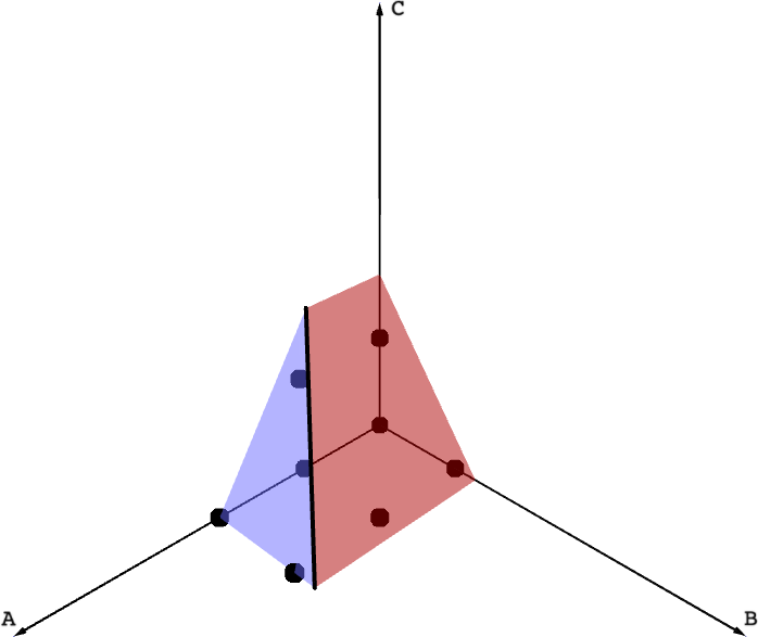
In this paper we derive in Theorem 6.1 an explicit formula for for all whenever is a triangulation that has a single totally interior edge – that is, an edge connecting two interior vertices. See Figure 1 for such a triangulation. A more intuitive version of our main result, described in terms of lattice points in a certain polytope, appears in Theorem 4.1. Our formula applies to any choice of vertex coordinates for , and only depends on the number of distinct slopes of edges meeting at each interior vertex. This is the first non-trivial dimension formula for planar splines that applies in this level of generality (all and any choice of vertex coordinates) since Schumaker computed the formula for splines on a planar vertex star in 1979 [25].
Our work directly extends results in previous papers of Tohǎneanu, Mináč, and Sorokina [29, 18, 27] which study the dimension of splines on a particular triangulation with a single totally interior edge. As a consequence of our work, we see that Schenck’s ‘’ conjecture is satisfied for triangulations with a single totally interior edge for all (Corollary 4.3). Moreover, it is clear from our result that the dimension of splines on a triangulation with a single totally interior edge only depends on local geometry and not global geometry. Thus the dependence of upon global geometry indicated by the Morgan-Scott split does not manifest unless there is more than one totally interior edge.
We briefly outline the paper. In Section 2 we recall background on splines and dimension formulas from previous papers. Section 3 is a largely technical section in which we prove a few results in commutative algebra, possibly of independent interest, for use in future sections. We then prove the first formulation of our main result – Theorem 4.1 – in Section 4, stated in terms of lattice points. In Section 5 we characterize in what degrees the spline space does not change upon removal of the totally interior edge (this is related to the phenomenon of supersmoothness explored in [27]). We give the fully explicit dimension formula in Theorem 6.1 of Section 6 and illustrate the result with several examples. We conclude with additional remarks and open problems in Section 7.
2. Splines on planar triangulations
We call a domain polygonal if it consists of a simple closed polygon and its interior. The simple closed polygon is the boundary of , which we denote by . Throughout this paper we assume is a triangulation of a polygonal domain; we denote the domain which triangulates by . For our purposes, a triangulation consists of a collection of triangles in which each pair of triangles satisfies or is either an edge or vertex of both and . Specifically, we do not allow so-called ‘hanging vertices’ which occur in the interior of an edge of a triangle.
We write for the set of vertices of , for the set of edges of , and for the set of triangles of . An interior edge of is an edge that is a common edge of two triangles of . A boundary edge of is an edge that is only contained in a single triangle of . An interior vertex of is a vertex that is not contained in any boundary edges. Put and for the set of interior vertices and interior edges of , respectively. A totally interior edge of is an edge that connects two interior vertices of .
Let be an integer. We define to be the set of -differentiable piecewise polynomial functions on . These functions are called splines. More explicitly:
Definition 2.1.
is the set of functions such that:
-
(1)
For all facets , is a polynomial in .
-
(2)
is differentiable of order .
For each integer , we define
For an edge , we write for a choice of affine linear form that vanishes on the affine span of .
Proposition 2.1 (Algebraic spline criterion).
[4, Corollary 1.3] Suppose is a triangulation of a polygonal domain and is a piecewise polynomial function. Then if and only if
for every pair so that .
The space is a finite dimensional -vector space. One of the key problems in spline theory is
Key Problem 1.
Determine for all .
To study this problem, we use a standard coning construction due to Billera and Rose [4]. Namely, for any set , define by . Define to be the tetrahedral complex whose tetrahedra are . All above definitions for triangulations in carry over in the expected way to tetrahedral complexes in . For a two-dimensional face , we write for the linear form defining the linear span of (this linear form is the homogenization of the affine linear form ). We put
where is the vector space of homogeneous polynomials of degree . We relate this space to using:
Proposition 2.2.
[4, Theorem 2.6] The real vector spaces and are isomorphic.
Along with the coning construction, we use the Billera-Schenck-Stillman (BSS) chain complex over . This chain complex is introduced by Billera in [3] and modified by Schenck and Stillman in [21].
Definition 2.2.
For an edge and vertex , define
-
•
(the principal ideal of generated by ) and
-
•
(the ideal of generated by .
Let . We define the chain complex by
where the differentials and are the differentials in the simplicial chain complex of relative to with coefficients in . In other words, the th homology is isomorphic to , where the latter is the th simplicial homology group of relative to with coefficients in . We also define the subcomplex by
and the quotient complex (which we call the Billera-Schenck-Stillman chain complex)
We use the following result of Schenck and Stillman.
It is shown in [20] that Schumaker’s lower bound – first derived using methods from numerical analysis in [25] – is the Euler characteristic of in degree . From this perspective, we give an explicit formula for for use later in the paper. We set some additional notation. If are non-negative integers, we use the following convention for the binomial coefficient :
For each vertex we let be the number of slopes of edges containing . Let and be the quotient and remainder when is divided by ; that is, , with and . Put . Then we have the following formula for .
Proposition 2.4.
Using the above notation, Schumaker’s lower bound for can be expressed as
We will occasionally consider splines on a partition which is not a triangulation but a rectilinear partition – in this case the polygonal domain is subdivided into polygonal cells which meet along edges. All definitions and results stated thus far carry over to rectilinear partitions. The class of rectilinear partitions we will have occcasion to use are called quasi-cross-cut partitions.
Definition 2.3.
A rectilinear partition is a quasi-cross-cut partition if every edge of is connected to the boundary of by a sequence of adjacent edges that all have the same slope.
The following result was first proved by Chui and Wang [5]; we give the formulation of the result that appears in [20].
Proposition 2.5.
If is a quasi-cross-cut partition then for all .
2.1. Case of a single totally interior edge
In this section we specialize to the case of interest in this paper. That is, is a triangulation with only two interior vertices and connected by a single totally interior edge . There are two cases in which the dimension formula on such a triangulation is trivial, which we record in the following proposition.
Proposition 2.6.
Let be a triangulation with a single totally interior edge connecting interior vertices and . Suppose that either
-
•
the interior edge has the same slope as another edge meeting at either or or
-
•
the number of slopes of edges meeting at either or is at least .
Then for all integers .
Proof.
The result follows from [20, Theorem 5.2]. In either case, and is a free module over the polynomial ring. ∎
Assumptions 2.1.
In the remainder of the paper, we use the following notation and assumptions whenever we have a triangulation with a single totally interior edge connecting interior vertices and .
-
•
We assume no edge adjacent to or has the same slope as .
-
•
We write (respectively ) for the number of edges different from which are adjacent to (respectively ).
-
•
We write (respectively ) for the number of different slopes achieved by the edges different from which contain (respectively ).
-
•
We assume (without loss) that .
Remark 1.
We explain the last bullet point in Assumptions 2.1. Since we assume no other edge besides has a slope equal to the slope of , is surrounded by edges taking on different slopes and is surrounded by edges taking on different slopes. See Figure 1. We obtain by simply relabeling and if necessary. If then either or . In either case it is not possible for to be a triangulation. (If it would be possible to have a so-called -juncture or ‘hanging vertex’ at , but we do not allow these under our definition of a triangulation.) Hence . We can also assume that and are both at most by Proposition 2.6. Putting these all together, we arrive at .
With this setup, consider the homology module where is the Billera-Schenck-Stillman chain complex. It turns out that is graded isomorphic to a shift of the quotient of the polynomial ring by an ideal.
Lemma 2.7.
If has only one totally interior edge , then
| (2) |
where
| (3) |
This lemma is a consequence of presentation for due to Schenck and Stillman. We recall this presentation before proceeding to the proof.
Lemma 2.8.
[21, Lemma 3.8] Let be the free module with summands indexed by the formal basis symbols which each have degree . Define to be the submodule of generated by
and, for each ,
The -module is given by generators and relations by
Proof of Lemma 2.7.
First, since has no holes, . This follows from the long exact sequence in homology associated to the short exact sequence of chain complexes and the fact that (see [21]).
Thus we may use Lemma 2.8. Since has only one totally interior edge , is generated by the free module and the syzygy modules for . Since all factors of indexed by an interior edge different from are quotiented out, after trimming the presentation in Lemma 2.8 we are left with
where . Observe that is the internal sum of the submodules
for , where Thus . Recalling that has degree , this proves that
After coning, we apply a change of coordinates so that points in the direction of and points in the direction of . With respect to this new choice of coordinates we may choose linear forms vanishing on the interior codimension one faces so that:
In Section 3 we study ideals of this type, returning to the study of the homology module in Section 4.
3. The initial ideal of a power ideal in two variables
This section is largely a technical section in which we derive some results from commutative algebra – possibly of independent interest – to use in our analysis for in future sections. The reader will not lose much by skipping this section for now and returning later as needed or desired.
Suppose we are given a set of points , where for , and a sequence of multiplicities for these points. We will assume that the points are ordered so that . We associate two ideals to this set of points. First, the power ideal
in the polynomial ring (the offset by one in the exponent will make statements later a bit cleaner). Secondly, the fat point ideal
in the polynomial ring ( is the coordinate ring of ). The ideal consists of all polynomials which vanish to order at , for .
Our objective is to show that, under the assumption that for , the initial ideal with respect to either graded lexicographic or graded reverse lexicographic order, is a lex-segment ideal. Since the graded lexicographic and graded reverse lexicographic order coincide in two variables, we focus on the lexicographic order since it is consistent with the lex-segment definition.
Definition 3.1.
A monomial ideal is called a lex-segment ideal if, whenever a monomial of degree satisfies for some monomial of degree , then .
Lex-segment ideals play an important role in Macaulay’s classification of Hilbert functions [16]. Before proceeding to the proof, we introduce the notion of apolarity. An excellent survey of this notion by Geramita can be found in [11]. Define an action of on by
and extend linearly. That is, acts on as partial differential operators. It is straightforward to see that this action induces a perfect pairing
via . For an -vector subspace we thus define
Write for the -vector space spanned by homogeneous polynomials in of degree (this definition clearly extends to any homogeneous ideal). A result of Emsalem and Iarrobino describes in terms of fat point ideals. In the statement of the result below, we put and .
Theorem 3.1 (Emsalem and Iarrobino [9]).
As a corollary, the Hilbert function can be derived.
Corollary 3.2 (Geramita and Schenck [12]).
This shows that the Hilbert function of has the maximal growth possible for its number of generators. We take this analysis one step further.
Corollary 3.3.
Suppose that no point of has a vanishing -coordinate. Then the initial ideal is a lex-segment ideal.
Proof.
Fix a degree . Put and . By assumption, for any , so the monomial appears with non-zero coefficient in .
Since is principle, a basis for is given by
(Coupled with Theorem 3.1, this proves that , which is Corollary 3.2.) Observe that the given basis for has a polynomial whose lex-last term involves the monomial for .
If then . So suppose and that the leading term of some polynomial with respect to lex order is for some and . Then every other term of involves a power of which is larger than . From our above observation, the lex-last (or lex-least) monomial in the basis polynomial is . Thus . In fact, , so we can compute it exactly as:
which is non-zero because the ’s are all non-vanishing and . This contradicts Theorem 3.1, since but .
It follows that the initial terms of can only involve the monomials , where . Since by Corollary 3.2, it follows that consists of the lex-largest monomials of degree . Thus is a lex-segment ideal. ∎
In the following corollary we use the ordering .
Corollary 3.4.
With the same setup as Corollary 3.3, The initial ideal consists of the monomials , where , , and one of the strict inequalities , , is satisfied.
Proof.
It suffices to show that if and only if and is satisfied for every .
Since is a lex-segment ideal with Hilbert function , if and only if
Since it is not possible that . So we are left with the condition
Now, since , . The ‘plus’ subscript means only positive contributions to the sum on the right hand side are taken. So we can interpret the above inequality as
Equivalently, is satisfied for . Re-arranging, we get if and only if for . ∎
Remark 2.
Given non-negative integers , the inequalities , , and for define a convex polygon in . Corollary 3.4 says that the initial ideal of consists of monomials which are in bijection with the lattice points in the first quadrant of and are additionally not contained in this polygon. Equivalently, the monomials which are not in the initial ideal of are in bijection with the lattice points of this polygon.
In the next result, and following, if is a non-negative integer we write and for the case where consists of copies of .
Corollary 3.5.
With the same setup as Corollary 3.3, the initial ideal consists of those monomials satisfying , and .
Proof.
Due to Corollary 3.4, it suffices to show that the inequality is implied by the inequality for any . This is clear by multiplying both sides of by . ∎
3.1. Behavior under colon
In this section we discuss the behavior of under coloning with a power of . We continue to assume that no point of has a vanishing -coordinate. We use the following fact about graded reverse lexicographic order.
Proposition 3.6.
If under graded reverse lexicographic order, then . In particular, for any integer , .
Proof.
This is a special case of [8, Proposition 15.12]. ∎
Corollary 3.7.
For any integer , is a lex-segment ideal with Hilbert function
The monomial is in if and only if , and the inequality is satisfied for some .
Proof.
Due to Proposition 3.6 and the fact that graded lexicographic and graded reverse lexicographic orders coincide in two variables, we have . Now, a well-known identity is that . Said otherwise, the monomials in of degree are in bijection with the monomials of degree in which are divisible by . Since is spanned by lex-largest monomials, is either empty or consists of the lex-largest monomials of degree . This establishes both that is lex-segment and the claimed form of the Hilbert function.
For the description of the monomials which are in , it suffices to observe that if and only if . Then apply Corollary 3.4. ∎
3.2. A summation property of Gröbner bases
We would like to prove a general fact, which will be useful in later sections. We refer the reader to [6, Chapter 2] for basics on Gröbner bases and the Buchberger algorithm, and we follow the same notation.
Lemma 3.8.
Let be the polynomial ring . Assume is a homogeneous ideal generated by polynomials in the variables and and is a homogeneous ideal generated by polynomials in the variables and , then a Gröbner basis for with respect to graded lexicographic (or graded reverse lexicographic) order can be obtained by taking the union of the Gröbner bases of and with respect to the graded lexicographic (or graded reverse lexicographic) order. In particular, .
Proof.
Let be a Gröbner basis for and be a Gröbner basis for , both taken with respect to either graded lexicographic order or graded reverse lexicographic order. It suffices to show that satisfies Buchberger’s criterion - that is, the -pair of any two reduces to zero under the division algorithm. This is clearly true if both and are in or both and are in . So we assume . We further assume the leading coefficients of and are normalized to . Let and . Then
Put and . Assume (the case is entirely analogous). Then
where and are both polynomials because every term of is divisible by (and hence since ) and every term of is divisible by . There is no cancellation between the lead terms of and since the lead term of has a higher power of in it than . Thus . Since and ,
is what is called a standard representation of in [6, Section 9]. It is shown in [6, Section 9] that if every -pair of has a standard representation, then is a Gröbner basis, and so the result follows. ∎
4. The dimension formula expressed via lattice points
In this section we prove our first version of the dimension formula for when is a triangulation with a single totally interior edge. We also characterize when begins to agree with Schumaker’s lower bound. We record these as two separate results, and prove them at the very end of the section.
Theorem 4.1.
Let be a triangulation with a single totally interior edge satisfying Assumptions 2.1. Then for all integers ,
where and is the polytope in defined by , and . Equivalently, for all integers ,
where is the polygon in defined by the inequalities , , , and .
Theorem 4.2.
Let be a triangulation with a single totally interior edge satisfying Assumptions 2.1. If and then
Otherwise,
Remark 3.
Corollary 4.3.
We shall use Theorem 2.3 to prove Theorems 4.1 and 4.2, hence we spend the remainder of this section analyzing the homology module , where is the Billera-Schenck-Stillman chain complex from Section 2. We use Assumptions 2.1 throughout this section. As we observed in Section 2.1, we may change coordinates so that
Using Lemma 2.7, Proposition 3.6, and Lemma 3.8, we obtain the following corollary.
Corollary 4.4.
With the above definition of , and ,
| (4) |
and
| (5) |
where the initial ideal is taken with respect to graded lexicographic order or graded reverse lexicographic order.
Proof.
Lemma 4.5.
A basis for as an -vector space is given by the monomials which satisfy the inequalities and .
Proof.
A common use of initial ideals is that the monomials outside of form a basis for [6, Section 5.3]. Thus it suffices to show that if and only if satisfy the claimed inequalities. Since by (5), it suffices to show that and if and only if the claimed inequalities hold. Since the initial ideals are monomial, and . Thus we reduce in both cases to two variables, and the result now follows from Corollary 3.7. ∎
Example 4.1.
Let be the triangulation in Figure 1, with and . When , a basis for as an -vector space is given by the monomials which satisfy and . The lattice points satisfying these inequalities are shown in Figure 2. When , there is a single lattice point – – that satisfies these inequalites (see the plot at right in Figure 2). Thus and .
Proposition 4.6.
The dimension of in degree is given by the number of lattice points satisfying the inequalities , , , and .
Proof.
If is a graded module of finite length, recall that the (Castelnuovo-Mumford) regularity of , written , is defined by .
Proposition 4.7.
The regularity of is bounded by
| (6) |
More precisely,
| (7) |
Thus for , where is Schumaker’s lower bound [25].
To prove Proposition 4.7, we use the following lemma:
Lemma 4.8.
Assume . Let be the polytope in defined by the inequalities and . Let be the plane defined by . Then if and only if and . Moreover, if and then
-
•
If then
-
•
If then
Proof.
We first treat the case and . Assume . If , then and . Hence, , contradiction. Therefore, .
Next, we show that . Let . Substituting to , we know that must satisfy and . Eliminating and simplifying, we obtain
where and . Because and , so . Since and , this implies .
Therefore, , and hence and . Observe that if or then . Therefore if then and which in turn happens if and only if and . In case both congruences are satisfied, it is clear from the above reasoning that is the only point in .
Now we treat the case . First suppose is odd, so for some integer . Then and the polytope is defined by , , , , and . From the final two inequalities we deduce that and thus is empty. Now suppose for some integer . Then again, and is defined by the inequalities , , , , and . From , , and , we deduce that . Since and , we deduce that . ∎
Now we are ready to prove Proposition 4.7.
Proof of Proposition 4.7.
We first prove the bounds (6). By Lemma 2.7, the regularity of is the largest degree of a monomial in . By Lemma 4.5, if and . In particular, and satisfy this condition. By Lemma 2.7, we obtain
Note that the region of bounded by inequalities in Lemma 4.5 is a polytope, which we denote by as in Lemma 4.8. Thus the largest degree of a monomial in is obtained by maximizing the linear functional over . It is well-known in linear programming that the maximum of this linear functional on occurs at one of the vertices of . Therefore, to prove the upper bound, it suffices to verify that evaluating at the vertices achieves a value of at most . The vertices of have coordinates
respectively. Computing for each of them, we have
respectively. We want to show that
is the largest among all of them.
It is clear that
and that
We only need to show that
| (8) |
We have
Because , so , where equality holds if and only if . If , then equality in (8) holds. Otherwise, and
Thus, we have proved (8). This means
Therefore, the inequality (6) holds.
Example 4.2.
Assume that and . Then
and
Therefore,
Clearly every monomial of degree two or more is in , but the monomial is not in this ideal. Therefore and so by Lemma 2.7. The bounds given by (6) are
In this case, , so by Proposition 4.7, , which aligns with what we have found already.
On the other hand, if and , then
and
Therefore,
We can see by inspection that any monomial of degree five or more is in , while is a monomial of degree four not in this ideal. Thus and so, by Lemma 2.7, . In this case, (6) specializes to . Since and , Proposition 4.7 yields , which aligns with what we found by inspection.
Proof of Theorem 4.1.
5. Comparison to quasi-cross-cut
In this section we address the phenomenon that, for certain pairs , where is obtained by removing the unique totally interior edge from to get a quasi-cross-cut partition (see Definition 2.3), as shown in Figure 3.
In [27], Sorokina discusses this phenomenon using the Bernstein-Bézier form in the case (which she calls the Tohǎneanu partition due to its appearance in [29]). A main result of [27] is that for when . In this section, we extend Sorokina’s result to arbitrary and . This equality of dimensions upon removal of an edge is related to the phenomenon of supersmoothness [27, 10], although we will not go into details about this.
Let be a triangulation with a single totally interior edge and let be the partition formed by removing the edge from as in Figure 3. As in Section 4, put for . Furthermore, for any homogeneous ideal , define
Lemma 5.1.
There is a short exact sequence
| (9) |
where is the natural inclusion and is the difference of restricted to the faces and shown in Figure 3. In particular, if then .
Proof.
We prove that (9) is a short exact sequence; the final statement follows immediately. Let be the totally interior edge of , with corresponding linear form . Let be the linear forms defining the edges which surround the interior vertex , in clockwise order. Likewise suppose that the linear forms defining the edges which surround the interior vertex in counterclockwise order are . See Figure 3, where the edges are labeled by the corresponding linear forms. With this convention, , , and .
It is clear that is the kernel of the map . It follows from the algebraic spline criterion that if then . We show that is surjective. Suppose that . We define a spline so that as follows. Let and . Write for the remaining faces surrounding the vertex (in clockwise order) and for the remaining faces surrounding the vertex (in counterclockwise order). See Figure 3.
Then the linear forms defining the interior edges adjacent to are and for and the linear forms defining the interior edges adjacent to are and for .
Now we continue to define . Since for some polynomials . Define by for . Likewise, since , for some polynomials . Define by for . One readily checks, using Proposition 2.1, that . Clearly , so we are done. ∎
Since is principal, and . Hence, the .
Lemma 5.2.
For , let . We have
Moreover, the monomial if and only if , , and .
Proof.
The second part follows immediately from Corollary 3.7. So we only verify the first part. It is clear that . We only need to show that for all degrees .
By Corollary 4.4, we know that . We also know that for any ideal . Because
and
we must have for all degree . This completes the proof. ∎
Corollary 5.3.
Let be a triangulation with a single totally interior edge satisfying Assumptions 2.1. For , .
Proof.
As in Lemma 5.2, we let for . By Lemma 5.1, it suffices to prove that . From the discussion just prior to Lemma 5.2 coupled with the lemma itself, it suffices to prove that .
Let be the collection of points defined by the inequalities , and . Then its closure (in the usual topology on ) is the polyhedron in defined by the inequalities , and . Using Lemma 5.2 again,
We first show that is the smallest value achieved by on the polyhedron . Since we assume that , it is not possible for any to satisfy or . The vertices of the polyhedron are:
We have proved (8), which implies that evaluated at is at least as large as evaluated at . Since , evaluated at is at most evaluated at . Therefore, over the real numbers, is minimized over at the vertex , with a value of . Let be the affine hyperplane defined by . A straightforward calculation with the inequalities also shows that , hence and also . It follows that
6. The explicit dimension formula
In this section we use the preceding sections to give an explicit formula for , where is a planar triangulation with a single totally interior edge, for any and . We then illustrate the formula in a few examples.
Theorem 6.1.
Let be a triangulation with a single totally interior edge satisfying Assumptions 2.1 and the partition formed by removing . Then
where
Moreover, put . If , , and , then . Otherwise .
Proof.
First, it follows from that Now, if then by Corollary 5.3. Since is a quasi-cross-cut partition, it follows from Proposition 2.5 that for all .
Likewise, if then by Theorem 4.2. Observe that these first two cases allow us to dispense of the case (which we consider in more detail in Example 6.1). So henceforth we assume .
According to Theorem 4.1, it remains to show that, when , , where is the polytope defined by the inequalities , , , , and .
We first show that, in the given range for , is in fact a triangle bounded by , , and . For this observe that
from which we deduce that . Since , we need only show that . Re-arranging, we see this is equivalent to
which is precisely our assumption. So is a consequence of and . Since , we obtain
or . Using the given bound on , we obtain . Since , we thus have and so .
It follows that is the triangle in the first quadrant bounded by , , and . Now we count the lattice points . We do this by counting the lattice points on the line segments defined by the intersection of with , for . The two lines defined by the equations and intersect at the point
where (restricted to ) achieves its minimum value of
Thus we start our count at , which is the lower index of summation for the definition of in the theorem statement. Clearly the maximum is .
Now put , so . We have
yielding or . Likewise we have
which yields or . Putting these together, the number of lattice points with is the same as the number of integers in the interval
which is counted by
Summing this over the appropriate range for yields the expression for .
In the following examples we compute explicit formulas for certain triangulations with a single totally interior edge. We assume that the triangulation satisfies Assumptions 2.1 and we introduce some additional notation to explicitly write out Schumaker’s lower bound. Let and (respectively and ) be the quotient and remainder when is divided by (respectively is divided by ). That is, and , where and . Furthermore, put and . From Proposition 2.4 we have
| (10) |
Now let and (respectively and ) be the quotient and remainder when is divided by (respectively is divided by ). That is, and , where and . Furthermore, put and . Again from Proposition 2.4 we have
| (11) |
Example 6.1.
Consider the triangulation with and . Sorokina calls this a Tohǎneanu partition in [27] due to its study by Tohǎneanu in [29] and [18]. According to Theorem 6.1, we have
The first case (for ) recovers [27, Theorem 3.1]. The second case (for ) recovers the main result of [18]. From Equation (11) we have
Since the final term of vanishes for , we have for , recovering [27, Theorem 3.2]. When is odd (), Equation (10) yields
and when is even (), Equation (10) yields
If (), then
and if (), then
This proves that , so Schumaker’s lower bound indeed does not give the correct dimension for (the inequality also follows from an application of Theorem 4.2). This recovers the main result of [29].
Example 6.2.
Consider the triangulation shown in Figure 1, with and . If then is free and for all integers by Proposition 2.6. For , according to Theorem 6.1, for and for . For ,
We now use Equations (10) and (11) to compute dimension formulas for . When , we have
When ,
which simply means that the triangle defined by the inequalities in Proposition 4.6 does not contain any lattice points. Thus . This also is expected by Theorem 6.1 since and .
Observing that the last three terms of vanish when , we conclude that
When , there is no integer so that , so we simply have
When , we hit our first non-zero contribution from . Namely, when , (this comes from the single lattice point pictured on the right in Figure 2). Notice that , so we must compute directly. Thus
Remark 4.
The smallest values of , , , and where we see a non-zero contribution from in Theorem 6.1 are , and , where .
7. Concluding remarks and open problems
We close with a number of remarks on connections to the literature and open problems.
Remark 5.
It should be possible to use our techniques to analyze additional ‘supersmoothness’ across the totally interior edge, as Sorokina does in [27].
Remark 6.
We can apply the methods of this paper to determine whenever the only non-trivial generators of correspond to totally interior edges which do not meet each other. In this case the dimension of would be obtained by simply adding together the contributions from the different totally interior edges.
Remark 7.
The next natural case in which to compute for all is the case when has two totally interior edges which meet at a vertex.
Problem 1.
Suppose is a triangulation with two totally interior edges which meet at a common vertex. Find a formula for for all , and all choices of vertex coordinates.
The recent counterexample to Schenck’s ‘’ conjecture in [32, 22] is a triangulation with two totally interior edges which meet at a vertex. Thus, contrary to our result for triangulations with a single totally interior edge in Corollary 4.3, we might not have for when is a triangulation with two totally interior edges meeting at a vertex.
Remark 8.
The well-known Morgan-Scott split, for which depends on the global geometry of , has three totally interior edges which form a triangle. In a remarkable preprint, Whiteley shows that the process of vertex splitting applied to the Morgan-Scott split leads to infinitely many triangulations for which the dimension of quadratic splines depends on global geometry [30]. Vertex splitting results in a triangulation with additional triangles all of whose edges are totally interior edges. As far as we are aware, the Morgan-Scott split and its vertex splits are the only known triangulations for which the dimension of quadratic splines exhibits a dependence upon global, as oppoosed to local, geometry. For each , there is a variation of the Morgan-Scott split so that exhibits dependence on global geometry [15]. Each of these has three totally interior edges forming a triangle as well. Given that Theorem 6.1 implies that a triangulation with a single totally interior edge depends only on local geometry, we pose Problem 2.
Problem 2.
If no triangle of is surrounded by totally interior edges – equivalently, the dual graph has no interior vertex – does the dimension of depend only on local geometry (that is, the number of slopes meeting at each interior vertex)?
Remark 9.
If is a rectilinear partition, a mixed spline space on , written , is one where different orders of smoothness are imposed across different edges according to a function . Generally speaking, decreasing the order of smoothness across certain edges of a partition enriches the resulting spline space, while increasing the smoothness coarsens the spline space.
In [7] it is shown that the (Castelnuovo-Mumford) regularity of the mixed spline space on a rectilinear partition can be bounded by the maximum regularity of the space of mixed splines on the union of two adjacent polygonal cells of –that is, the star of an edge –where vanishing is imposed (to the order prescribed by ) across all edges which the polygonal cells do not have in common. It may be possible that the methods of this paper can be used to improve the regularity bounds derived in [7] for mixed splines on the star of an edge with vanishing imposed across the boundary. Improving the regularity bound for splines on the star of an edge with vanishing across the boundary will give a better bound on the degree needed for the formula to stabilize.
Remark 10.
A generalized quasi-cross-cut partition (see [17]) is defined as follows. We call a sequence of adjacent edges of a cross-cut if they all have the same slope and both endpoints of the sequence touch the boundary of . We call a sequence of adjacent edges of a quasi-cross-cut if all edges have the same slope, one endpoint of the sequence touches the boundary, and the other endpoint cannot be extended to include another adjacent edge of the same slope. It is possible that a cross-cut or quasi-cross-cut consists of only a single edge – for instance, any edge which is not totally interior is either a quasi-cross-cut or it can be extended to a quasi-cross-cut. For a vertex , we define to be the number of cross-cuts passing through and to be the number of quasi-cross-cuts passing through . The rectilinear partition is a generalized quasi-cross-cut partition if for every . Generalized quasi-cross-cut partitions are studied by Manni in [17] and Shi, Wang, and Yin in [26].
If has a single totally interior edge, it is clearly a generalized quasi-cross-cut partition. If has a single totally interior edge connecting vertices and with different slopes meeting at and different slopes meeting at , it follows from [17, Theorem 2.2] that for and from [26, Theorem 5] that for . Theorem 4.2 shows an improvement on both of these bounds. This leads us to pose Problem 3, inspired by the result of Shi, Wang, and Yin and our Theorem 4.2.
Problem 3.
If is a generalized quasi-cross-cut partition, define for each edge the quantity . Let . Is it true that for ?
If Problem 3 has a positive answer, it would imply that all generalized quasi-cross-cut partitions satisfy Schenck’s ‘’ conjecture (and the conjecture of Alfeld and Manni for ). Notice that the only known counterexample to Schenck’s conjecture in [32, 22] is not a generalized quasi-cross-cut partition since the central vertex has only a single cross-cut passing through it, and no quasi-cross-cuts.
Acknowledgements
The core ideas that led to this paper can be found in a preprint of the second author: An upper bound on the regularity of the first homology of spline complexes https://arxiv.org/pdf/1907.10811.pdf. The current paper extends these ideas to give a complete dimension formula. The authors participate in a semi-regular virtual meeting on topics related to splines along with Peter Alfeld, Tatyana Sorokina, Nelly Villamizar, Maritza Sirvent, and Walter Whiteley. This meeting facilitated our collaboration, and we are grateful to all members of this group for their comments on this work and many inspiring discussions.
References
- [1] P. Alfeld. Multivariate splines and the Bernstein-Bézier form of a polynomial. Computer Aided Geometric Design, 45:2–13, 2016.
- [2] P. Alfeld and L. Schumaker. On the dimension of bivariate spline spaces of smoothness and degree . Numerische Mathematik, 57(1):651–661, 1990.
- [3] L. Billera. Homology of smooth splines: generic triangulations and a conjecture of Strang. Transactions of the American Mathematical Society, 310(1):325–340, 1988.
- [4] L. Billera and L. Rose. A dimension series for multivariate splines. Discrete & Computational Geometry, 6(1):107–128, 1991.
- [5] C. Chui and R. Wang. Multivariate spline spaces. J. Math. Anal. Appl., 94(1):197–221, 1983.
- [6] D. Cox, J. Little, and D. O’Shea. Ideals, varieties, and algorithms. Undergraduate Texts in Mathematics. Springer, Cham, fourth edition, 2015. An introduction to computational algebraic geometry and commutative algebra.
- [7] M. DiPasquale. Dimension of mixed splines on polytopal cells. Math. Comp., 87(310):905–939, 2018.
- [8] D. Eisenbud. Commutative Algebra: with a view toward algebraic geometry, volume 150. Springer Science & Business Media, 2013.
- [9] J. Emsalem and A. Iarrobino. Inverse system of a symbolic power, i. Journal of Algebra, 174(3):1080–1090, 1995.
- [10] M. Floater and K. Hu. A characterization of supersmoothness of multivariate splines. Adv. Comput. Math., 46(5):Paper No. 70, 15, 2020.
- [11] A. Geramita. Inverse systems of fat points: Waring’s problem, secant varieties of Veronese varieties and parameter spaces for Gorenstein ideals. In The Curves Seminar at Queen’s, Vol. X (Kingston, ON, 1995), volume 102 of Queen’s Papers in Pure and Appl. Math., pages 2–114. Queen’s Univ., Kingston, ON, 1996.
- [12] A. Geramita and H. Schenck. Fat points, inverse systems, and piecewise polynomial functions. Journal of Algebra, 204(1):116–128, 1998.
- [13] D. Hong. Spaces of bivariate spline functions over triangulation. Approx. Theory Appl., 7(1):56–75, 1991.
- [14] M. Lai and L. Schumaker. Spline functions on triangulations, volume 110 of Encyclopedia of Mathematics and its Applications. Cambridge University Press, Cambridge, 2007.
- [15] Z. Luo, F. Liu, and X. Shi. On singularity of spline space over Morgan-Scott’s type partition J. Math. Res. Exposition, 30(1):1–16, 2010.
- [16] F. Macaulay. Some Properties of Enumeration in the Theory of Modular Systems. Proc. London Math. Soc. (2), 26:531–555, 1927.
- [17] C. Manni. On the dimension of bivariate spline spaces on generalized quasi-cross-cut partitions. Journal of Approximation Theory, 69(2):141–155, 1992.
- [18] J. Mináč and S. Tohǎneanu. From spline approximation to Roth’s equation and Schur functors. Manuscripta Mathematica, 142(1-2):101–126, 2013.
- [19] H. Schenck. Algebraic methods in approximation theory. Computer Aided Geometric Design, 45:14–31, 2016.
- [20] H. Schenck and M. Stillman. A family of ideals of minimal regularity and the Hilbert series of . Advances in Applied Mathematics, 19(2):169–182, 1997.
- [21] H. Schenck and M. Stillman. Local cohomology of bivariate splines. Journal of Pure and Applied Algebra, 117:535–548, 1997.
- [22] H. Schenck, M. Stillman, and B. Yuan. A new bound for smooth spline spaces. J. Comb. Algebra, 4(4):359–367, 2020.
- [23] H. Schenck and P. Stiller. Cohomology vanishing and a problem in approximation theory. Manuscripta Mathematica, 107(1):43–58, 2002.
- [24] H. Schenck. Homological methods in the theory of splines. ProQuest LLC, Ann Arbor, MI, 1997. Thesis (Ph.D.)–Cornell University.
- [25] L. Schumaker. On the dimension of spaces of piecewise polynomials in two variables. In Multivariate approximation theory, pages 396–412. Springer, 1979.
- [26] X. Shi, T. Wang, and B. Yin. Splines on generalized quasi-cross-cut partitions. J. Comput. Appl. Math., 96(2):139–147, 1998.
- [27] T. Sorokina. Bivariate splines on Tohǎneanu partition. Journal of Approximation Theory, 232:6–11, 2018.
- [28] G. Strang. Piecewise polynomials and the finite element method. Bull. Amer. Math. Soc., 79:1128–1137, 1973.
- [29] Ş. Tohǎneanu. Smooth planar -splines of degree . Journal of Approximation Theory, 132(1):72–76, 2005.
- [30] W. Whiteley. The geometry of bivariate splines. 1990.
- [31] W. Whiteley. The combinatorics of bivariate splines. In Applied geometry and discrete mathematics, volume 4 of DIMACS Ser. Discrete Math. Theoret. Comput. Sci., pages 587–608. Amer. Math. Soc., Providence, RI, 1991.
- [32] B. Yuan and M. Stillman. A counter-example to the Schenck-Stiller “” conjecture. Advances in Applied Mathematics, 110:33–41, 2019.