Efficient subsampling for exponential family models

Abstract

We propose a novel two-stage subsampling algorithm based on optimal design principles. In the first stage, we use a density-based clustering algorithm to identify an approximating design space for the predictors from an initial subsample. Next, we determine an optimal approximate design on this design space. Finally, we use matrix distances such as the Procrustes, Frobenius, and square-root distance to define the remaining subsample, such that its points are “closest” to the support points of the optimal design. Our approach reflects the specific nature of the information matrix as a weighted sum of non-negative definite Fisher information matrices evaluated at the design points and applies to a large class of regression models including models where the Fisher information is of rank larger than $1$.

Keywords: Subsampling, optimal design, exponential family, matrix distances

1 Introduction

Nowadays, with the easy accessibility to data collecting frameworks and computing devices, a large amount of data is encountered in various fields ranging from terrestrial data, manufacturing sector, and e-commerce to name a few. Training statistical models to draw inferences with such large volumes of data can be very time-consuming. A popular method for dealing with large-scale data is sampling, where one performs statistical inference on a subsample, which (hopefully) represents the most informative part of the data and is used as a surrogate.

Various subsampling algorithms have been proposed in recent times for this purpose using concepts of optimal design theory. Some of the algorithms perform probability-based sampling based on minimizing variances of the predicted response or of the estimator (see, for example Ma et al.,, 2015; Wang et al.,, 2018). The others are deterministic (see, for example Wang et al.,, 2019, 2021; Ren and Zhao,, 2021).

The IBOSS algorithm (Wang et al.,, 2019) applies to (homoscedastic) linear regression and determines the most informative points by component-wise selecting extreme covariate values. Simulation studies show that it is an improvement over the leverage-based algorithm. Wang et al., (2021) and Ren and Zhao, (2021) consider also the linear regression model and use the concept of orthogonal arrays to construct subsampling procedures. An orthogonal array ensures that the covariates are as far apart as possible and also supports the selection of extreme values. As a result, these authors demonstrate by means of a simulation study that orthogonal array-based subsampling is an improvement over IBOSS. Cheng et al., (2020) extend the IBOSS approach to define a deterministic subsampling procedure for the logistic regression.

Several non-deterministic subsampling procedures have been developed for these regression models as well. For example, Ma et al., (2015) gives a leverage-based algorithm for linear regression, that performs a probability-based subsample with replacement based on the leverage scores of each data point. Wang et al., (2018) considers two-stage subsampling algorithms for the logistic regression model, where the first stage consists in taking a random sample, which is used to obtain a preliminary estimate of the parameter. They then propose a probability score (depending on the initial estimate of the parameter in stage I) based subsampling with replacement based on the A-optimality criterion. It has been improved by Wang, (2019) and extended to several other models and estimation techniques (see Wang and Ma,, 2020; Ai et al.,, 2021; Yu et al.,, 2022, among others). In principle, these non-deterministic methods apply to a broad class of regression models and we refer to the recent review paper by Yao and Wang, (2021) for the current state of the art.

In this paper, we propose a new deterministic subsampling algorithm that can also be easily applied to a wide class of regression models. In contrast to the currently available methods, which are based on specific properties of the regression model (such as, it is reasonable to use observations with large components in homoscedastic linear regression) our approach uses basic principles of optimal design theory and is generally applicable. Our general idea is to interpret the sampling as an optimal design problem. For this purpose, the proposed algorithm first tries to understand the nature/shape of the design space which, roughly speaking, is the domain containing most of the predictors of the sample. Thereafter, we determine a subsample approximating the optimal design on the identified design space. More precisely, in the first step, we obtain an initial parameter estimate (if necessary) and determine an approximation of the design space using a density-based clustering algorithm. Next, we determine the optimal design on the “estimated design space”. When the number of support points of the optimal design is large, we use the concept of efficiency to eliminate the most unimportant points from the optimal design, which ensures much less execution time for the subsequent subsampling step. To identify the points in the subsample, which are “closest” to the remaining support points of the optimal design, we use matrix distances such as the Procrustes, Frobenius, and square-root distance (see, for example, Dryden et al.,, 2009; Pigoli et al.,, 2014, for a definition).

The algorithm, which is most similar in spirit is the subsampling procedure proposed recently by Deldossi and Tommasi, (2022) and also accounts for the shape of the design space. Our approach differs from this work with respect to at least three perspectives. First, these authors propose to determine an optimal design (more precisely its weights) using the full sample as design space, which is computationally expensive for large-scale data. In contrast, our approach applies clustering techniques to determine a (discrete) design space from an initial subsample (which is also used to obtain initial estimates of the parameter). It is therefore computationally much cheaper because the cardinality of the estimated design space is substantially smaller than the size of the total sample. Second, it is robust with respect to outliers due to density based clusters identifying the design space. Third, we propose to utilize the geometry of the space induced by the Fisher information matrix and thus use matrix distances on the space of non-negative definite matrices (see Dryden et al.,, 2009; Pigoli et al.,, 2014) to identify the remaining points for the subsample, such that they are close to the support points of the optimal design. This reflects the specific nature of the information matrix which is a weighted sum of the non-negative definite Fisher information matrices evaluated at the design points. As a consequence, our approach is applicable for regression models where the Fisher information is of rank larger than $1$, as they appear, for example, in heteroscedastic regression models (see Atkinson and Cook,, 1995; Dette and Holland-Letz,, 2009)

The rest of the paper is organized in the following way: Section 2 discusses the models under consideration and the idea of approximate optimal design. The subsampling algorithm is introduced in Section 3. Finally, we demonstrate in Section 4 through simulation studies that the new approach has better accuracy compared to existing subsampling approaches proposed in Cheng et al., (2020) and Wang et al., (2018) in the case of a logistic regression model. Compared to the optimal design-based subsampling approach proposed in Deldossi and Tommasi, (2022), our approach has improved time complexities. In this section, we also illustrate the applicability of our subsampling approach to a heteroskedastic regression model, where the Fisher information has rank larger than $1$.

2 Preliminaries

We assume that the full data sample $\mathcal{D}=\{(\boldsymbol{x}_{i},y_{i}):i=1,\ldots,n\}$ are realization of i.i.d. $\mathbb{R}^{p+1}$-dimensional random variables with (conditional) distribution from an exponential family with density (with respect to a dominating measure, say $\nu$ defined on an appropriate sigma field)

$$f(y|\boldsymbol{x},\boldsymbol{\beta}) =h(y)\;\exp\{\eta^{\top}(\boldsymbol{x},\boldsymbol{\beta})T(y)-A(\boldsymbol{x},\boldsymbol{\beta})\},$$ (2.1)

where ($\boldsymbol{x}$,$y$) is defined on ${\cal X}\times{\cal Y}\subset\mathbb{R}^{p+1}$, $\boldsymbol{\beta}=(\beta_{0},\beta_{1},\ldots,\beta_{p})^{\top}\in\Theta\subset\mathbb{R}^{p+1}$ denotes the unknown vector of parameters, $\boldsymbol{x}$ is a $p$-dimensional predictor and $y$ a univariate response. Here, $h(y)$ is assumed to be a positive measurable function, $\eta:{\cal X}\times\Theta\to\mathbb{R}^{l}$, $A:{\cal X}\times\Theta\to\mathbb{R}$, and $T$ denote a $l$-dimensional statistic.

We denote by $\hat{\boldsymbol{\beta}}=(\hat{\beta}_{0},\hat{\beta}_{1},\ldots,\hat{\beta}_{p})^{\top}\in\mathbb{R}^{p+1}$ the maximum likelihood estimate of the parameter $\boldsymbol{\beta}$ from the full sample $\mathcal{D}$ and recall that under standard regularity assumptions (see, for example, Theorem 5.1 in Lehmann and Casella,, 2006) the statistic $(\mathcal{I}(\boldsymbol{\beta},\boldsymbol{X}))^{-1/2}\big{(}\hat{\boldsymbol{\beta}}-\boldsymbol{\beta}\big{)}$ is asymptotically normal distributed with mean vector $0$ and covariance matrix $I_{p+1}$, where $\mathcal{I}(\boldsymbol{\beta},\boldsymbol{X})$ denotes the information matrix defined by

$$\mathcal{I}(\boldsymbol{\beta},\boldsymbol{X}) =\sum_{i=1}^{n}\mathcal{I}(\boldsymbol{\beta},\boldsymbol{x}_{i}),$$ (2.2)

$\boldsymbol{X}=[{\boldsymbol{x}}_{1},\ldots,{\boldsymbol{x}}_{n}]^{\top}$ and

$$\mathcal{I}(\boldsymbol{\beta},\boldsymbol{x}) =\mathbb{E}\Big{[}\Big{\{}\dfrac{\partial\log f(y|\boldsymbol{x},\boldsymbol{\beta})}{\partial\boldsymbol{\beta}}\Big{\}}^{\top}\;\;\Big{\{}\dfrac{\partial\log f(y|\boldsymbol{x},\boldsymbol{\beta})}{\partial\boldsymbol{\beta}}\Big{\}}\Big{]}$$ (2.3)

is the Fisher information matrix at the point $\boldsymbol{x}$. We are interested in identifying a most informative subsample from ${\cal D}$ of size $k$, say

$$\mathcal{D}_{k} =\{(\boldsymbol{x}_{s_{i}},y_{s_{i}}):i=1,\ldots,k\}\leavevmode\nobreak\ \subset\leavevmode\nobreak\ \mathcal{D}.$$

and denote by $\hat{\boldsymbol{\beta}}_{\mathcal{D}_{k}}$ the parameter estimate based on the subsample $\mathcal{D}_{k}$. Before we continue, we present three examples, which will be in the focus of this paper.

Example 2.1.

Assume that ${\cal Y}=\mathbb{R}$, $\nu$ is the Lebesgue measure, and that $g({\boldsymbol{x},\boldsymbol{\beta}})$ is a sufficiently smooth function. Then, for

$$h(y)=\dfrac{\exp{(-{y}^{2}/2\sigma^{2})}}{\sqrt{2\pi\sigma^{2}}},\leavevmode\nobreak\ \eta(\boldsymbol{x},\boldsymbol{\beta})=\dfrac{g({\boldsymbol{x},\boldsymbol{\beta}})}{\sigma^{2}},\leavevmode\nobreak\ T(y)=y,\leavevmode\nobreak\ A(\boldsymbol{x},\boldsymbol{\beta})=\dfrac{g({\boldsymbol{x},\boldsymbol{\beta}})^{2}}{2\sigma^{2}}$$

we obtain the normal distribution (with known variance $\sigma^{2}$) and the common nonlinear regression model with

$$\mathbb{E}[y|\boldsymbol{x},\boldsymbol{\beta}]=g({\boldsymbol{x},\boldsymbol{\beta}})\leavevmode\nobreak\ .$$

Here the Fisher-information matrix for the parameter $\boldsymbol{\beta}$ at the point $\boldsymbol{x}$ is given by

$$\mathcal{I}(\boldsymbol{\beta},\boldsymbol{x}) =\dfrac{\partial g(\boldsymbol{x},\boldsymbol{\beta})^{\top}}{\partial\boldsymbol{\beta}}\;\dfrac{\partial g(\boldsymbol{x},\boldsymbol{\beta})}{\partial\boldsymbol{\beta}}.$$ (2.4)

In particular, if $g(\boldsymbol{x},\boldsymbol{\beta})=f(\boldsymbol{x})^{\top}\boldsymbol{\beta}$ for a $(p+1)$-dimensional vector of regression functions $f$, this model reduces to the common linear regression model. In this case, the Fisher-information at the point $\boldsymbol{x}$ is given by $\mathcal{I}(\boldsymbol{\beta},\boldsymbol{x})=f(\boldsymbol{x})f^{\top}(\boldsymbol{x})$.

Example 2.2.

If ${\cal Y}=\{0,1\}$, $\nu$ is the counting measure and

$$h(y) =1,\leavevmode\nobreak\ \eta(\boldsymbol{x},\boldsymbol{\beta})=\log\big{[}\pi(\boldsymbol{x},\boldsymbol{\beta})/(1-\pi(\boldsymbol{x},\boldsymbol{\beta})\big{]},$$

$$T(y) =y,\leavevmode\nobreak\ A(\boldsymbol{x},\boldsymbol{\beta})=-\log(1-\pi(\boldsymbol{x},\boldsymbol{\beta}))$$

for some function $\boldsymbol{x}\to\pi(\boldsymbol{x},\boldsymbol{\beta})\in(0,1)$, we obtain the Binomial response model, that is

$$f(y_{i}|\boldsymbol{x}_{i},\boldsymbol{\beta})=\pi(\boldsymbol{x}_{i},\boldsymbol{\beta})^{y_{i}}\big{(}1-\pi(\boldsymbol{x}_{i},\boldsymbol{\beta})\big{)}^{1-y_{i}}\leavevmode\nobreak\ ,$$ (2.5)

and

$$\mathbb{P}(y=1|\boldsymbol{x},\beta)=\pi(\boldsymbol{x},\boldsymbol{\beta}).$$ (2.6)

For the special choice

$$\pi(\boldsymbol{x},\boldsymbol{\beta})=\frac{\exp(\boldsymbol{z}^{\top}\boldsymbol{\beta})}{1+\exp(\boldsymbol{z}^{\top}\boldsymbol{\beta})}$$

where $\boldsymbol{z}=(1,\boldsymbol{x}^{\top})^{\top}$ we get the frequently used logistic regression model with parameter $\boldsymbol{\beta}$. In this case, the Fisher-information at the point $\boldsymbol{x}$ is given by

$$\mathcal{I}(\boldsymbol{\beta},\boldsymbol{x}) =\big{(}\phi(\boldsymbol{z},\boldsymbol{\beta})\boldsymbol{z}\big{)}\;\;\big{(}\phi(\boldsymbol{z},\boldsymbol{\beta})\boldsymbol{z}\big{)}^{\top},$$ (2.7)

where

$$\phi(\boldsymbol{z},\boldsymbol{\beta})=\displaystyle{\dfrac{\exp(\boldsymbol{z}^{\top}\boldsymbol{\beta}/2)}{1+\exp(\boldsymbol{z}^{\top}\boldsymbol{\beta})}}.$$

Example 2.3.

Assume that ${\cal Y}=\mathbb{R}$, $\nu$ is the Lebesgue measure, and that $g({\boldsymbol{x},\boldsymbol{\beta}})$ is a sufficiently smooth function. Then, for $T(y)=\big{[}y^{2}\leavevmode\nobreak\ \leavevmode\nobreak\ y\big{]}^{\top},\leavevmode\nobreak\$

$$h(y)=\dfrac{1}{\sqrt{2\pi}},\leavevmode\nobreak\ \eta(\boldsymbol{x},\boldsymbol{\beta})=\Big{[}\dfrac{-1}{2\sigma^{2}({\boldsymbol{x},\boldsymbol{\beta}})}\leavevmode\nobreak\ \leavevmode\nobreak\ \dfrac{g({\boldsymbol{x},\boldsymbol{\beta}})}{\sigma^{2}({\boldsymbol{x},\boldsymbol{\beta}})}\Big{]}^{\top},\leavevmode\nobreak\ A(\boldsymbol{x},\boldsymbol{\beta})=\dfrac{g^{2}({\boldsymbol{x},\boldsymbol{\beta}})}{2\sigma^{2}({\boldsymbol{x},\boldsymbol{\beta}})}-\dfrac{1}{2}\log(\sigma^{2}({\boldsymbol{x},\boldsymbol{\beta}}))$$

we obtain the normal distribution and the common heteroskedastic nonlinear regression model with

$$\mathbb{E}[y|\boldsymbol{x},\boldsymbol{\beta}] =g({\boldsymbol{x},\boldsymbol{\beta}})\leavevmode\nobreak\ ,\leavevmode\nobreak\ \leavevmode\nobreak\ {\rm Var}[y|\boldsymbol{x},\boldsymbol{\beta}]=\sigma^{2}({\boldsymbol{x},\boldsymbol{\beta}}).$$ (2.8)

In this case, Fisher-information matrix for the parameter $\boldsymbol{\beta}$ at the point $\boldsymbol{x}$ is given by

$$\mathcal{I}(\boldsymbol{\beta},\boldsymbol{x}) =\dfrac{1}{\sigma^{2}({\boldsymbol{x},\boldsymbol{\beta}})}\dfrac{\partial g(\boldsymbol{x},\boldsymbol{\beta})^{\top}}{\partial\boldsymbol{\beta}}\;\dfrac{\partial g(\boldsymbol{x},\boldsymbol{\beta})}{\partial\boldsymbol{\beta}}+\dfrac{1}{2\sigma^{4}({\boldsymbol{x},\boldsymbol{\beta}})}\dfrac{\partial\sigma^{2}({\boldsymbol{x},\boldsymbol{\beta}})^{\top}}{\partial\boldsymbol{\beta}}\;\dfrac{\partial{\sigma^{2}({\boldsymbol{x},\boldsymbol{\beta}})}}{\partial\boldsymbol{\beta}}$$ (2.9)

(see Dette and Holland-Letz,, 2009). Note that in general the matrix in (2.9) has rank $2$ (in contrast to Example 2.1 and 2.2).

In the following, we will develop an algorithm for selecting a subsample $\mathcal{D}_{k}$ from $\cal D$ such that the resulting maximum likelihood estimator $\hat{\boldsymbol{\beta}}_{\mathcal{D}_{k}}$ based on ${{\mathcal{D}_{k}}}$ is most efficient. Similar to Deldossi and Tommasi, (2022) the subsampling algorithm proposed in this article is based on optimal design principles. For this purpose, we briefly describe some basic facts from optimal design theory (see, for example, the monographs of Silvey,, 1980; Pukelsheim,, 2006; Randall et al.,, 2007, for more details) and present some tools, which will be useful for our approach. Following Kiefer, (1974) we define an approximate design $\xi$ on a given design space ${\cal X}$ (which will be determined as described in Section 3.2 below) as a probability measure with weights $w_{1},\ldots,w_{d}$ at the points ${\boldsymbol{x}}_{1},\ldots,{\boldsymbol{x}}_{d}\in{\cal X}$. If $N$ observations can be taken, the quantities ${w}_{\ell}N$ are rounded to non-negative integers, say $N_{\ell}$, such that $\sum_{\ell=1}^{d}N_{\ell}=N$ and the experimenter takes $N_{\ell}$ (independent) observations at each ${\boldsymbol{x}}_{\ell}$ ($\ell=1,\ldots,d$). In this case, under standard assumptions, the covariance matrix of the maximum likelihood estimator $\sqrt{N}\hat{\boldsymbol{\beta}}$ for the parameter ${\boldsymbol{\beta}}$ in model (2.1) converges to the matrix $M^{-1}(\xi,\boldsymbol{\beta})$, where

$$M(\xi,\boldsymbol{\beta}):=\sum_{i=1}^{d}w_{i}\mathcal{I}(\boldsymbol{\beta},\boldsymbol{x}_{i}),$$

which is the analog of the matrix (2.2) and used to measure the accuracy of the estimator $\hat{\boldsymbol{\beta}}$. An optimal design maximizes an appropriate functional, say $\Psi$, of the matrix $M(\xi,\boldsymbol{\beta})$ with respect to the design $\xi$. Here $\Psi$ is an information function in the sense of Pukelsheim, (2006), that is a positively homogeneous, concave, non-negative, non-constant, and upper semi-continuous function on the space of non-negative definite matrices and the optimal design is called $\Psi$-optimal design. Numerous criteria have been proposed in the literature to discriminate between competing designs (see Pukelsheim,, 2006) and we exemplary mention Kiefer’s $\Psi_{q}$-criteria, which are defined for $-\infty\leq q<1$ as

$$\Psi_{q}(\xi)=(\text{tr}\big{\{}\big{(}M^{q}(\xi,\boldsymbol{\beta})\big{\}}\big{)}^{1/q} =\Big{(}\text{tr}\Big{\{}\Big{(}\sum_{i=1}^{d}w_{i}\mathcal{I}(\boldsymbol{\beta},\boldsymbol{x}_{i})\Big{)}^{q}\Big{\}}\Big{)}^{1/q},$$ (2.10)

and contain the famous $E$-optimality $(q=-\infty)$, $A$-optimality $(q=-1)$ and $D$-optimality $(q=0)$ criterion as special cases. Under some continuity assumptions a $\Psi$-optimal design, say

$$\xi^{\ast}(\boldsymbol{\beta},{\boldsymbol{\chi}})=\biggl{\{}\genfrac{}{}{0.0pt}{}{{\boldsymbol{x}}_{1}^{\ast}}{w^{\ast}_{1}}\;\genfrac{}{}{0.0pt}{}{{\boldsymbol{x}}_{2}^{\ast}}{w^{\ast}_{2}}\ldots\genfrac{}{}{0.0pt}{}{{\boldsymbol{x}}_{d}^{\ast}}{w^{\ast}_{d}}\biggl{\}},$$

maximizing (2.10) exists, where ${\boldsymbol{x}}_{1}^{\ast},{\boldsymbol{x}}_{2}^{\ast},\ldots,{\boldsymbol{x}}_{d}^{\ast}\in{\boldsymbol{\chi}}$ and $w^{\ast}_{1}+w^{\ast}_{2}+\ldots+w^{\ast}_{d}=1$ are the support points and weights of the optimal design. Note that in general, this design depends on the unknown parameter $\boldsymbol{\beta}$ and on the design space ${\cal X}$, which is reflected in our notation. Of course, the design also depends on the optimality criterion $\Psi$. However, as the criterion does not play an important role in the following discussion (in fact the proposed method is basically applicable for any information function in the sense of Pukelsheim, (2006)), this dependence will not be reflected in the following discussion.

In most cases of practical interest, a $\Psi$-optimal design is unknown and has to be found numerically, and for a given design $\xi$ its $\Psi$-efficiency is defined by

$$\mbox{eff}(\xi,\boldsymbol{\beta})={\Psi(M(\xi,\boldsymbol{\beta}))\over\Psi(M(\xi^{\ast}(\boldsymbol{\beta},{\boldsymbol{\chi}}),\boldsymbol{\beta}))}\in[0,1]$$ (2.11)

3 Optimal Design Based Sub-sampling

In this section, we explain the basic structure of the proposed algorithm to obtain a subsample of size $k$, which is called ODBSS and summarized in Algorithm 1: first, we use an initial sample to obtain an estimate of a design space and of the parameter $\boldsymbol{\beta}$. Second, based on the estimated design space and the parameter estimate, we determine the (locally) optimal design with respect to some optimality criterion. Third, we determine a subsample by choosing the data points, which are close to the support points of the optimal design. For this purpose, we will define an appropriate “metric” on the set $\boldsymbol{\chi}$.

Before we give details for each step in Section 3.1 - 3.3, we illustrate our approach in a concrete example. In Figure 1, we display a typical situation, where we use ODBSS to determine a subsample for estimating the parameter of a logistic regression model with $p=2$ parameters, and where the true parameter is given by $\boldsymbol{\beta}=(0.1,0.5,0.5)$. The full sample size is $n=50000$ and we want to find the most informative subsample of size $k=5000$. Figure 1(a) displays the corresponding predictors simulated from a $2$-dimensional normal distribution centered at $(0,0)^{\top}$ with unit variances and correlation $0.5$. Figure 1(b) displays predictors corresponding to the initial subsample of size $k_{0}=1000$, which is chosen by uniform random sampling. This initial subsample $\mathcal{D}_{k_{0}}$ is used for two purposes: first, to obtain an initial parameter estimate (say $\hat{\boldsymbol{\beta}}_{\mathcal{D}_{k_{0}}}$) for the parameter $\boldsymbol{\beta}$, and second, to get an estimate of a “design space” (say ${{\boldsymbol{\chi}}}_{k_{0}}$), which is used in the calculations for obtaining the optimal design. Figure 1(c) shows the estimated design space ${{\boldsymbol{\chi}}}_{k_{0}}$ and the support points of the $A$-optimal design $\xi^{\ast}(\hat{\boldsymbol{\beta}}_{\mathcal{D}_{k_{0}}},{{\boldsymbol{\chi}}}_{k_{0}})$ on the design space ${{\boldsymbol{\chi}}}_{k_{0}}$. The details of design space estimation and optimal design determination can be found in Section 3.1 and 3.2, respectively. Finally, Figure 1(d) shows the $k-k_{0}$ (=4000) optimal subsample points, such that they are in some sense close to the support points of the optimal design $\xi^{\ast}(\hat{\boldsymbol{\beta}}_{\mathcal{D}_{k_{0}}},{{\boldsymbol{\chi}}}_{k_{0}})$ (see the right lower panel, and Section 3.3 for more details).

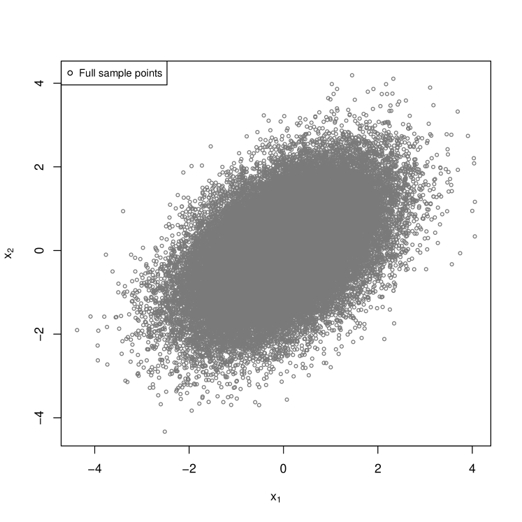
(a) Covariates of full data $(n=50000)$.

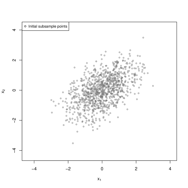
(b) Initial uniform subsample ($k_{0}=1000$).

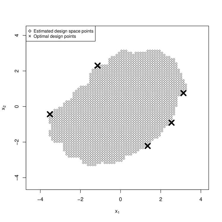
(c) Estimated design space and optimal approximate design.

(d) Final ODBSS subsample($k=5000$)

Figure 1: Illustration of key steps in ODBSS algorithm for a logistic regression model.

Algorithm 1 ODBSS

Input: The sample $\mathcal{D}$ of size $n$

• Initial sampling

  • Take a uniform subsample of size $k_{0}$ denoted by $\mathcal{D}_{{k_{0}}}$

  • Find an estimate of the design space ${{\boldsymbol{\chi}}}_{k_{0}}$ based on $\mathcal{D}_{{k_{0}}}$

  • Calculate an initial parameter estimate $\hat{\boldsymbol{\beta}}_{\mathcal{D}_{k_{0}}}$ based on $\mathcal{D}_{{k_{0}}}$

• Optimal design determination

  Find a (locally) approximate optimal design $\xi^{\ast}(\hat{\boldsymbol{\beta}}_{\mathcal{D}_{k_{0}}},{{\boldsymbol{\chi}}}_{k_{0}})$ on the design space ${{\boldsymbol{\chi}}}_{k_{0}}$ for the parameter $\hat{\boldsymbol{\beta}}_{\mathcal{D}_{k_{0}}}$.

• Optimal design based sampling

  • Determine the remaining subsample $\mathcal{D}_{{k_{1}}}$ ($k_{1}=k-k_{0}$), such that, $\lfloor w^{\ast}_{i}\leavevmode\nobreak\ k_{1}\rfloor$ observations are “close” to the support points ${\boldsymbol{x}}_{i}^{\ast}$ of the optimal design $\xi^{\ast}(\hat{\boldsymbol{\beta}}_{\mathcal{D}_{k_{0}}},{{\boldsymbol{\chi}}}_{k_{0}})$ ($i=1,\ldots,d$).

  • The final subsample $\mathcal{D}_{{k}}=\mathcal{D}_{{k_{0}}}\cup\mathcal{D}_{{k_{1}}}$

Output: The subsample $\mathcal{D}_{{k}}$ of size $k$

Remark 3.1.

In cases, where the optimal design does not depend on the parameter (for example in linear models) the parameter estimation in step (1) of Algorithm 1 is not necessary (but the design space has still to be estimated). Moreover, we emphasize that the points of the optimal design calculated in step (2) of Algorithm 1 are not necessarily part of the original sample $\mathcal{D}$.

3.1 Step 1: Estimation of the design space

To obtain the required design space ${\boldsymbol{\chi}}_{k_{0}}$ from the the initial set $\mathcal{D}_{{k_{0}}}$ we view it as a union of clusters and use the set of clusters in $\mathcal{D}_{{k_{0}}}$ to estimate ${\boldsymbol{\chi}}_{k_{0}}$. We found that a density-based clustering algorithm popularly referred to as DBSCAN (Ester et al.,, 1996) is suitable for our problem. In the following we describe the two main steps for design space estimation using DBSCAN.

1. Training DBSCAN from the initial sample ${\mathcal{D}}_{k_{0}}$. DBSCAN identifies several clusters labeled by $1,2,\ldots,m$ and a cluster of “outliers” labeled by $0$ using two inputs: a constant $\epsilon>0$ and an integer $m_{p}>0$. Consider first the case where there is only one cluster in $\mathcal{D}_{{k_{0}}}$. A point $\boldsymbol{c}\in\mathcal{D}_{{k_{0}}}$ is said to be a core point, if its $\epsilon$ neighbourhood $N_{\epsilon}(\boldsymbol{c})$ contains at least $m_{p}$ points from $\mathcal{D}_{{k_{0}}}$, that is $|N_{\epsilon}(\boldsymbol{c})\bigcap\mathcal{D}_{{k_{0}}}|\geq m_{p}$. A point $\boldsymbol{c}^{\prime}\in\mathcal{D}_{{k_{0}}}$ is said to be a boundary point, if $\boldsymbol{c}^{\prime}\in N_{\epsilon}(\boldsymbol{c})$ but $|N_{\epsilon}(\boldsymbol{c}^{\prime})\bigcap\mathcal{D}_{{k_{0}}}|<m_{p}$, where $\boldsymbol{c}$ is any core point. The cluster is the union of the core points and the boundary points. If there is more than one cluster present in the data, using a notion density reachability and density connectedness, this algorithm identifies the different clusters (for more details see Ester et al.,, 1996). We denote by $\mathcal{C}=\{C_{1},C_{2},\ldots,C_{m}\}$ the set of clusters present in the initial sample $\mathcal{D}_{{k_{0}}}$ and by $C_{0}$ the set of outliers.

2. Using DBSCAN for estimating a design space. Once the DBSCAN model is trained we can, in principle, decide for any $\boldsymbol{c}^{\prime\prime}\in\mathbb{R}^{p}$ if it belongs to a cluster from $\mathcal{C}$ or if it is an outlier. More precisely, if $\boldsymbol{c}^{\prime\prime}\in N_{\epsilon}(\boldsymbol{c})$ for some core point $\boldsymbol{c}\in\mathcal{D}_{{k_{0}}}$ associated with a cluster $C_{i}$, then $\boldsymbol{c}^{\prime\prime}\in{C}_{i}$. Thus, after training DBSCAN formally defines a function, which assigns each point to a cluster and, for a given set $\mathcal{M}\subset\mathbb{R}^{p}$, we obtain a decomposition

   $$\mathcal{M}=\mathcal{M}_{0}\cup\mathcal{M}_{1}\cup\mathcal{M}_{2}\cup\ldots\leavevmode\nobreak\ \cup\mathcal{M}_{m},$$

   where $\mathcal{M}_{j}$ contains the points in $\mathcal{M}$ which are assigned to $C_{j}$ $(j=1,\ldots,m)$. Note that $\mathcal{M}_{j}$ does not necessarily contain points from the cluster $C_{j}\subset\mathcal{D}_{k_{0}}$, it just contains all points from $\mathcal{M}$, which are “close” to the set $C_{j}$. We define for a set $\mathcal{M}\subset\mathbb{R}^{p}$ the function

   $$\Omega_{\mathcal{D}_{{k_{0}}}}(\mathcal{M})=\mathcal{M}_{1}\cup\ldots\cup\mathcal{M}_{m}\leavevmode\nobreak\ ,$$

   where the index $\mathcal{D}_{{k_{0}}}$ reflects the fact that the clusters are defined by the initial sample $\mathcal{D}_{{k_{0}}}$. We finally define the estimated design space by

   $${{\boldsymbol{\chi}}}_{k_{0}} =\Omega_{\mathcal{D}_{{k_{0}}}}(\mathcal{G})\leavevmode\nobreak\ ,$$ (3.1)

   where

   $$\mathcal{G} =\Big{\{}({i_{1}},\ldots,{i_{j}})^{\top}\leavevmode\nobreak\ \Big{|}\leavevmode\nobreak\ i_{j}\in\Big{\{}\underline{K}_{j},\tfrac{L\underline{K}_{j}+(\overline{K}_{j}-{\underline{K}_{j}})}{L},\ldots,\tfrac{L\underline{K}_{j}+(\overline{K}_{j}-{\underline{K}_{j}})(L-1)}{L},\overline{K}_{j}\Big{\}};\leavevmode\nobreak\ j=1,\ldots,p\Big{\}}\leavevmode\nobreak\$$

   is a grid and the bounds $\underline{K}_{1},\ldots,\underline{K}_{p}$ and $\overline{K}_{1},\ldots,\overline{K}_{p}$ are chosen such that the grid covers the covariate space corresponding to the initial sample $\mathcal{D}_{k_{0}}$ and $L$ corresponds to the partition size of the grid.

In our simulation studies, we use the R-implementation in the $dbscan$ package in $R$-software (see Hahsler et al.,, 2022), where $\epsilon$ is set to be equal to the maximum $4^{th}$ nearest neighbour distance of $\boldsymbol{x}\in\mathcal{D}_{k_{0}}$ and adjusted for outliers (a similar approach recommended in Ester et al.,, 1996) and $m_{p}=5$.

3.2 Step 2: Determination of the optimal design

For most cases of practical interest, the optimal designs have to be found numerically and for this purpose, we use the R-package OptimalDesign (see Harman and Lenka,, 2019). Note that only the optimal weights have to be determined, where most of the points in ${\boldsymbol{\chi}}_{k_{0}}$ will get weight $0$. The resulting optimal design will be denoted by

$$\xi^{\ast}(\hat{\boldsymbol{\beta}}_{\mathcal{D}_{k_{0}}},{{\boldsymbol{\chi}}}_{k_{0}})=\Big{\{}\genfrac{}{}{0.0pt}{}{{\boldsymbol{x}}_{1}^{\ast}}{w^{\ast}_{1}}\;\genfrac{}{}{0.0pt}{}{{\boldsymbol{x}}_{2}^{\ast}}{w^{\ast}_{2}}\leavevmode\nobreak\ \ldots\leavevmode\nobreak\ \genfrac{}{}{0.0pt}{}{{\boldsymbol{x}}_{d}^{\ast}}{w^{\ast}_{d}}\Big{\}},$$ (3.2)

where we assume without loss of generality that the weights are ordered, that is $w^{\ast}_{1}\geq{w^{\ast}_{2}}\geq\ldots\geq{w^{\ast}_{d}}$. For a large dimensional parameter, the number of support points of the optimal design is rather large, but in many cases, most of the mass is concentrated at a smaller number of support points. Because in Step (3) of Algorithm 1 we determine points in the sample $\mathcal{D}$ which are close to support points of the optimal design, we propose to reduce the number of support points by deleting support points with small weights as long as the efficiency of the design is not decreasing substantially. In other words, for a given efficiency bound $\zeta\in(0,1)$ we consecutively omit the support points with small weights in $\xi^{\ast}(\hat{\boldsymbol{\beta}}_{\mathcal{D}_{k_{0}}},{{\boldsymbol{\chi}}}_{k_{0}})$ (and rescale the weights) such that the resulting design has at least efficiency $\zeta$. The details are given in Algorithm 2 and in the following discussion the resulting design will also be denoted $\xi^{\ast}(\hat{\boldsymbol{\beta}}_{\mathcal{D}_{k_{0}}},{{\boldsymbol{\chi}}}_{k_{0}})$. In Section 4.1.3, we study the impact of this choice of $\zeta$ on the accuracy of the resulting subsampling in a logistic regression model. In particular, we demonstrate that the number of support points can be reduced substantially without losing too much efficiency.

Algorithm 2 Optimal design with reduced support points

Input: $\Psi$-optimal design $\xi^{\ast}=\xi^{\ast}(\hat{\boldsymbol{\beta}}_{\mathcal{D}_{k_{0}}},{{\boldsymbol{\chi}}}_{k_{0}})$ defined in (3.2); accuracy $\zeta\in(0.5,1)$

    Set ${d^{\prime}}={d}$ and $\xi^{\ast}_{d^{\prime}}=\xi^{\ast}(\hat{\boldsymbol{\beta}}_{\mathcal{D}_{k_{0}}},{{\boldsymbol{\chi}}}_{k_{0}})$

while $\Psi(\xi^{\ast}_{{d^{\prime}}})>\zeta\Psi(\xi^{\ast})$ and $d^{\prime}>p$ do

         ${d^{\prime}}\leftarrow{d^{\prime}}-1$

         $u^{\ast}_{i}\leftarrow\frac{w^{\ast}_{i}}{\sum^{d^{\prime}}_{i=1}w^{\ast}_{i}}$ (for $i=1,\ldots,d^{\prime}$)

         $w^{\ast}_{i}\leftarrow u^{\ast}_{i}$ (for $i=1,\ldots,d^{\prime}$)

         $\xi^{\ast}_{d^{\prime}}\leftarrow\Big{\{}\genfrac{}{}{0.0pt}{}{{\boldsymbol{x}}_{1}^{\ast}}{w^{\ast}_{1}}\;\genfrac{}{}{0.0pt}{}{{\boldsymbol{x}}_{2}^{\ast}}{w^{\ast}_{2}}\ldots\genfrac{}{}{0.0pt}{}{\boldsymbol{x}^{\ast}_{d^{\prime}}}{w^{\ast}_{d^{\prime}}}\Big{\}}$

end while$\xi^{\ast}(\hat{\boldsymbol{\beta}}_{\mathcal{D}_{k_{0}}},{{\boldsymbol{\chi}}}_{k_{0}})\leftarrow\xi^{\ast}_{d^{\prime}+1}$

Output: Design $\xi^{\ast}(\hat{\boldsymbol{\beta}}_{\mathcal{D}_{k_{0}}},{{\boldsymbol{\chi}}}_{k_{0}})$ with a minimal number of support points and $\Psi$-efficiency larger or equal than $\zeta$.

3.3 Step 3: Design based subsampling

Once the approximate $\Psi$-optimal design $\xi^{\ast}(\hat{\boldsymbol{\beta}}_{\mathcal{D}_{k_{0}}},{{\boldsymbol{\chi}}}_{k_{0}})$ has been determined (if necessary with a reduced number of support points), the algorithm proceeds to find the remaining $k_{1}=k-k_{0}$ points for the subsample such that they are close to the support points $\boldsymbol{x}_{1}^{*},\ldots,\boldsymbol{x}_{d}^{*}$ of the approximate $\Psi$-optimal design. For this purpose, we introduce several distances, which will be discussed first.

In particular, we are not comparing the points $\boldsymbol{x}$ and $\boldsymbol{x}^{\prime}$ with respect to a norm on $\boldsymbol{\chi}$. Instead, we use distances between the Fisher information matrices $\mathcal{I}(\boldsymbol{x})$ and $\mathcal{I}(\boldsymbol{x}^{\prime})$. We concentrate on the Frobenius distance

$$d_{F}(\boldsymbol{x},\boldsymbol{x}^{\prime}) :=\|\mathcal{I}(\boldsymbol{x})-\mathcal{I}(\boldsymbol{x}^{\prime})\|_{F}:=tr\Big{\{}\big{(}\mathcal{I}(\boldsymbol{x})-\mathcal{I}(\boldsymbol{x}^{\prime})\big{)}^{\top}\leavevmode\nobreak\ \big{(}\mathcal{I}(\boldsymbol{x})-\mathcal{I}(\boldsymbol{x}^{\prime})\big{)}\Big{\}}^{1/2}\leavevmode\nobreak\ ,$$ (3.3)

the square root distance

$$d_{s}(\boldsymbol{x},\boldsymbol{x}^{\prime}) :=\|\mathcal{I}(\boldsymbol{x})^{1/2}-\mathcal{I}(\boldsymbol{x}^{\prime})^{1/2}\|_{F}\leavevmode\nobreak\ ,and$$ (3.4)

and the Procrustes distance

$$d_{p}(\boldsymbol{x},\boldsymbol{x}^{\prime}) :=\displaystyle{\inf_{\boldsymbol{K}\in O(\mathbb{R}^{p\times p})}\Big{\{}\|\mathcal{I}(\boldsymbol{x})-\mathcal{I}(\boldsymbol{x}^{\prime})\boldsymbol{K}\|_{F}\Big{\}}^{1/2}}$$ (3.5)

between the information matrices $\mathcal{I}(\boldsymbol{x})$ and $\mathcal{I}(\boldsymbol{x}^{\prime})$, which reflect the geometry of the space $\{\mathcal{I}(\boldsymbol{x},\boldsymbol{\beta})\leavevmode\nobreak\ :\leavevmode\nobreak\ \boldsymbol{x}\in\boldsymbol{\chi}\}$ as a subset of the non-negative definite (symmetric) matrices (see Dryden et al.,, 2009; Pigoli et al.,, 2014). Here the infimum in (3.5) is taken over the set of all $p\times p$ orthogonal matrices. Note that the Procrustes distance can be further simplified if the Fisher information at $\boldsymbol{x}$ and $\boldsymbol{x}^{\prime}$ can be represented as $\mathcal{I}(\boldsymbol{x})=\boldsymbol{L}_{1}\boldsymbol{L}_{1}^{T}$ and $\mathcal{I}(\boldsymbol{x}^{\prime})=\boldsymbol{L}_{2}\boldsymbol{L}_{2}^{T}$, respectively. In this case we have $d_{p}^{2}(\boldsymbol{x},\boldsymbol{x}^{\prime})=\|\boldsymbol{L}_{1}\|_{F}^{2}+\|\boldsymbol{L}_{2}\|_{F}^{2}-2\Sigma_{k}\sigma_{k}$, where $\sigma_{1},\sigma_{2},\ldots,$ are the singular values of the matrix $\boldsymbol{L}_{2}^{T}\boldsymbol{L}_{1}$ (see Dryden et al.,, 2009; Pigoli et al.,, 2014).

We can use any of these distances (and also other distances) in step (3) of Algorithm 1 and in the following, we denote this distance by $d$. The points, which are closest to the support points of the optimal design $\xi^{\ast}(\hat{\boldsymbol{\beta}}_{\mathcal{D}_{k_{0}}},{{\boldsymbol{\chi}}}_{k_{0}})$ in (3.2) with respect to $d(\cdot)$ are retained in the subsample. The number of points corresponding to each design point $\boldsymbol{x}_{i}^{*}$ is proportional to the corresponding weight $w_{i}^{*}$, which means that only $\lfloor w^{\ast}_{i}\leavevmode\nobreak\ k_{1}\rfloor$ points closest to $\boldsymbol{x}_{i}$ (with respect to the distance $d(\cdot)$) are retained in the subsample. The details of distance-based subsample allocation are summarized in Algorithm 3.

Algorithm 3 Subsampling of the points closest to the support of the locally optimal design

Inputs: Sample $\mathcal{D}$, locally optimal design $\xi^{\ast}(\hat{\boldsymbol{\beta}}_{\mathcal{D}_{k_{0}}},{{\boldsymbol{\chi}}}_{k_{0}})$, and one of the distance metric $d(.)$ as defined in (3.3) - (3.5).

Define $\mathcal{D}_{k_{1}}=\emptyset$.

for  $i=1,\ldots,d$ do

     for  $j=1,\ldots,n$ do

          Calculate $d_{ij}=d({\boldsymbol{x}}_{i}^{\ast},{\boldsymbol{x}}_{j})$,

     end for

     Define $\boldsymbol{d}_{i}=(d_{i1},d_{i2},\ldots,d_{in})$

     Let $\boldsymbol{d}_{i_{(\cdot)}}=(d_{i{(1)}},d_{i_{(2)}},\ldots,d_{i_{(n)}})$, where ${\boldsymbol{d}_{i{(\cdot)}}}$ is the vector of ordered components of ${\boldsymbol{d}_{i}}$

     ($d_{i{(1)}}$ is the smallest value).

end for

for  $i=1,\ldots,d$ do

     From $\boldsymbol{d}_{i{(\cdot)}}$, remove all components corresponding to points in $\mathcal{D}_{k_{1}}$.

     Take sample points $\boldsymbol{x}\in\mathcal{D}$ corresponding to the first $\lfloor w^{\ast}_{i}\leavevmode\nobreak\ k_{1}\rfloor$ elements in $\boldsymbol{d}_{i{(\cdot)}}$ and add

     them to $\mathcal{D}_{k_{1}}$.

end for

Output: $\mathcal{D}_{k}=\mathcal{D}_{k_{0}}\cup\mathcal{D}_{k_{1}}$ is the subsample of size $k$

3.4 Computational complexity of ODBSS

In this section we briefly discuss the computational complexity of the ODBSS algorithm, which is constituted of three main parts:

1. Area estimation: The complexity of DBSCAN algorithm with $p$-dimensional $k_{0}$ points is $\mathcal{O}(k^{2}_{0}p)$ (see Schubert et al.,, 2017). Note that $k_{0}$ and $p$ are small compared to $n$.

2. Calculation of the $\Psi$-optimal design on the design space $\mathcal{X}_{k_{0}}$: The R-package OptimalDesign determines the optimal weights $w_{i}^{\ast}$ maximizing (2.10), but this time the points $\boldsymbol{x}_{i}$ of the estimated designs space $\mathcal{X}_{k_{0}}$ are candidates for the support of the design $\xi^{\ast}$. Sagnol and Harman, (2015) formulates the problem of finding approximate optimal design into a mixed integer second-order cone programming and discusses the time complexity for finding approximate optimal designs under various criteria. It can be seen that by using a second-order cone programming an approximate A-optimal design could be determined in time $\mathcal{O}(spr)^{3}\leavevmode\nobreak\ \sqrt{sp}\leavevmode\nobreak\ log(1/\epsilon)$, where $\epsilon$ is the permissible error, $s$ is the cardinality of $\mathcal{X}_{k_{0}}$, $r$ is the rank of the information matrix at a point defined in equation (2.3) (see also Ben-Tal and Nemirovski,, 2001, for more details on complexity for solving second order cone programming). From equation (3.1) we see that in Algorithm 1, in step (2) where the optimal design is determined, $s=|\mathcal{X}_{0}|\leq|\mathcal{G}|=L^{p}$. Therefore, the experimenter has control over the computation time for the determination of the optimal design by varying the grid size parameter $L$ as opposed to calculating the optimal design on the full sample.

3. Subsample allocation: For the subsample allocation the distances $\boldsymbol{d}_{i}$ for $i=1,\ldots,d$ needs to be computed and then $\lfloor w_{i}k_{1}\rfloor$ smallest elements $\boldsymbol{d}_{i}$ are determined (see Algorithm 3). In the case when the information matrix $\mathcal{I}(\boldsymbol{x},\boldsymbol{\beta})$ at point $\boldsymbol{x}$ has rank $1$, that is, in the case of usual logistic and linear regression, calculation of $\boldsymbol{d}_{i}$ has computational complexity $\mathcal{O}(dnp)$ and then determining $\lfloor w_{i}k_{1}\rfloor$ smallest elements $\boldsymbol{d}_{i}$ has complexity $\mathcal{O}(nd)$ (Martınez,, 2004). Therefore, the total computational complexity of this step of the Algorithm in the rank $1$ case is $\mathcal{O}(nd(p+1))$. To draw some comparisons we would highlight that, the time-complexity for IBOSS linear regression Wang et al., (2019) is $\mathcal{O}(np)$, IBOSS for logistic regression Cheng et al., (2020) is approximately $\mathcal{O}(np)$, and OSMAC for logistic regression Wang et al., (2018) is also $\mathcal{O}(np)$. Although this step is computationally more expensive, we emphasize that the algorithms proposed in these references are specifically constructed for the linear and logistic regression model, while OBDSS is generally applicable.

4 Numerical results

In this section, we investigate the performance of the new algorithm (ODBSS) by means of a small simulation study. In Section 4.1 we consider the logistic regression model (2.6), which corresponds to a Fisher information of rank $1$. We provide a comparison of versions of OBDSS with different distance metrics $d_{F}$, $d_{s}$ and $d_{p}$ as defined in (3.3), (3.4) and (3.5), respectively and also compare ODBSS with alternative subsampling algorithms for logistic regression (see Cheng et al.,, 2020; Wang et al.,, 2018). Moreover, we illustrate the effect of reducing support points of the optimal designon ODBSS (using Algorithm 3) and investigate the computational time of an alternative method for design space estimation (more precisely, using the full sample as an estimate of design space in step 1 of Algorithm 1 rather than a cluster-based area determination). Finally, Section 4.2 is devoted to the performance of ODBSS for a model with a Fisher information matrix of rank larger than $1$.

In the following illustrations, different subsample algorithms will be compared by the mean squared error

$$\mathbb{E}\big{[}\|\boldsymbol{\beta}-\hat{\boldsymbol{\beta}}_{\mathcal{D}_{k}}\|^{2}\big{]},$$ (4.1)

which is estimated by $100$ simulation runs. The full sample size is $n=100000$ and subsamples of size $k=1250,2500,$ and $5000$ are considered. All optimal designs are determined with respect to the $A$-optimality criterion.

Note, when the rank of the Fisher information matrix $\mathcal{I}(\boldsymbol{x},\boldsymbol{\beta})$ at point $\boldsymbol{x}$ is $1$, then

$$\mathcal{I}(\boldsymbol{x},\boldsymbol{\beta})=\Phi(\boldsymbol{x},\boldsymbol{\beta})\Phi(\boldsymbol{x},\boldsymbol{\beta})^{\top}$$

where $\Phi(\boldsymbol{x},\boldsymbol{\beta})\in\mathbb{R}^{p+1}$. In that case, calculating the matrix distances becomes very easy and we obtain

$$d_{F}(\boldsymbol{x},\boldsymbol{x}^{\prime}) =\Big{\{}\|\Phi(\boldsymbol{x},\boldsymbol{\beta})\|^{4}+\|\Phi(\boldsymbol{x}^{\prime},\boldsymbol{\beta})\|^{4}-2(\Phi(\boldsymbol{x}^{\prime},\boldsymbol{\beta})^{\top}\Phi(\boldsymbol{x},\boldsymbol{\beta}))^{2}\Big{\}}^{1/2},$$

$$d_{s}(\boldsymbol{x},\boldsymbol{x}^{\prime}) =\Big{\{}\|\Phi(\boldsymbol{x},\boldsymbol{\beta})\|^{2}+\|\Phi(\boldsymbol{x}^{\prime},\boldsymbol{\beta})\|^{2}-2\dfrac{(\Phi(\boldsymbol{x}^{\prime},\boldsymbol{\beta})^{\top}\Phi(\boldsymbol{x},\boldsymbol{\beta}))^{2}}{\|\Phi(\boldsymbol{x},\boldsymbol{\beta})\|\leavevmode\nobreak\ \|\Phi(\boldsymbol{x}^{\prime},\boldsymbol{\beta})\|}\Big{\}}^{1/2},$$

$$d_{p}(\boldsymbol{x},\boldsymbol{x}^{\prime}) =\|\Phi(\boldsymbol{x},\boldsymbol{\beta})-\Phi(\boldsymbol{x}^{\prime},\boldsymbol{\beta})\|=\Big{\{}\|\Phi(\boldsymbol{x},\boldsymbol{\beta})\|^{2}+\|\Phi(\boldsymbol{x}^{\prime},\boldsymbol{\beta})\|^{2}-2(\Phi(\boldsymbol{x}^{\prime},\boldsymbol{\beta})^{\top}\Phi(\boldsymbol{x},\boldsymbol{\beta}))\Big{\}}^{1/2},$$

where $\|\cdot\|$ is the Euclidean norm. However, no such simple representations exist in the case, where the rank of the information matrix $\mathcal{I}(\boldsymbol{x},\boldsymbol{\beta})$ is larger than $1$.

4.1 Logistic regression - rank $1$ case

We consider a logistic regression model of the form (2.6) with $p=7$ predictors and no intercept. The true value of the model parameter is set to ${\boldsymbol{\beta}}=(0.5,0.5,\ldots,0.5)^{\top}$. The covariates $\boldsymbol{x}=(x_{1},x_{2},\ldots,x_{7})^{\top}$ follows either centered a multivariate normal distribution with covariance $\boldsymbol{\Sigma}$ or a centered $t$-distribution with $\kappa$ degrees of freedom defined by its density

$$h(\boldsymbol{x}) =\dfrac{\Gamma[(\kappa+p)/2]}{\Gamma(\kappa/2)(\pi\kappa)^{p/2}{|\boldsymbol{\Sigma}|}^{1/2}}\Big{[}1+\dfrac{1}{\kappa}\boldsymbol{x}^{\top}\boldsymbol{\Sigma}^{-1}\boldsymbol{x}\Big{]}^{-(\kappa+p)/2}\leavevmode\nobreak\ ,$$

where we used $\kappa=3$ to study the effect of more heavy-tailed covariates. For both cases, we consider three types of covariance structures:

1. $\boldsymbol{\Sigma}_{1}=(0.5^{|i-j|})_{i,j=1,\ldots,7}$.

2. In each simulation run we choose randomly $5$ mutually orthogonal dominant directions $\boldsymbol{e}_{1}$, $\boldsymbol{e}_{2}$, $\boldsymbol{e}_{3}$, $\boldsymbol{e}_{4}$, and $\boldsymbol{e}_{5}$ $\in$ on $\mathbb{S}_{6}=\{\boldsymbol{x}\in\mathbb{R}^{7}\leavevmode\nobreak\ |\leavevmode\nobreak\ \|\boldsymbol{x}\|=1\}$ using the randortho-function in $R$. Then, the covariance matrix is defined by

   $${\boldsymbol{\Sigma}_{2}}=2\;\boldsymbol{e}_{1}\boldsymbol{e}_{1}^{\top}+1.8\;\boldsymbol{e}_{2}\boldsymbol{e}_{2}^{\top}+1.6\;\boldsymbol{e}_{3}\boldsymbol{e}_{3}^{\top}+1.4\;\boldsymbol{e}_{4}\boldsymbol{e}_{4}^{\top}+1.2\;\boldsymbol{e}_{5}\boldsymbol{e}_{5}^{\top}+0.1\;{\boldsymbol{\Sigma}_{1}}.$$

   where ${\boldsymbol{\Sigma}_{1}}$ is defined in (1). Note, that this data is concentrated in the neighborhood of a $5$-dimensional plane determined by the vectors $\boldsymbol{e}_{1},\boldsymbol{e}_{2},\boldsymbol{e}_{3},\boldsymbol{e}_{4}$ and $\boldsymbol{e}_{5}$.

3. Similarly, to (2) we consider data concentrating in a neighborhood of a $3$-dimensional plane. Thus we randomly choose in each run mutually orthogonal dominant directions $\boldsymbol{e}_{1}$, $\boldsymbol{e}_{2}$, and $\boldsymbol{e}_{3}$ $\in\mathbb{S}_{6}\subset\mathbb{R}^{7}$, and define

   $${\boldsymbol{\Sigma}_{3}}=3\;\boldsymbol{e}_{1}\boldsymbol{e}_{1}^{\top}+2\;\boldsymbol{e}_{2}\boldsymbol{e}_{2}^{\top}+1\;\boldsymbol{e}_{3}\boldsymbol{e}_{3}^{\top}+0.1\;{\boldsymbol{\Sigma}_{1}}.$$

4.1.1 The impact of different distances on ODBSS

In this section, we investigate the impact of the metric (step 3 of Algorithm 1) on the performance of ODBSS. More precisely, we display in Figure 2 the simulated mean squared error (MSE) of ODBSS, which is used with the different metrics $d_{F}$, $d_{s}$ and $d_{P}$ defined in (3.3), (3.4) and (3.5), respectively. For the sake of brevity, we restrict ourselves to the case of a normal distribution. The results for the $t$-distribution are very similar and not reported here. We observe that the three metrics do not yield substantial differences in ODBSS. Since there is not much difference in the performance of ODBSS for the different metrics in the logistic regression model, we use ODBSS with Frobenius distance $d_{F}(\cdot)$ in the following sections to illustrate other aspects of the ODBSS algorithm in the logistic regression model.

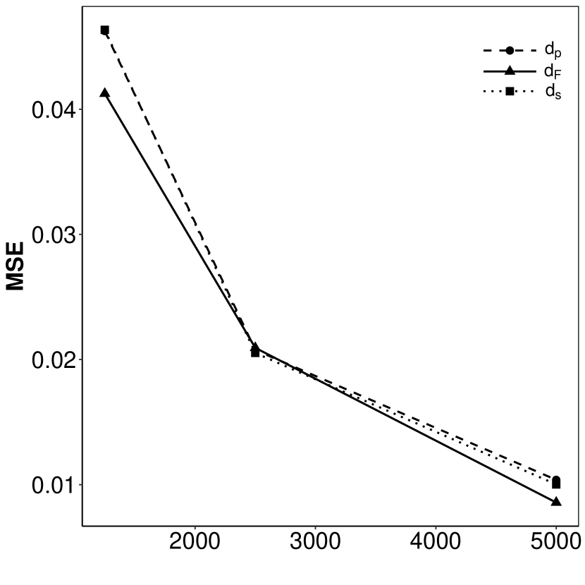
(a) $\mathcal{N}(\boldsymbol{0},{\boldsymbol{\Sigma}_{1}})$

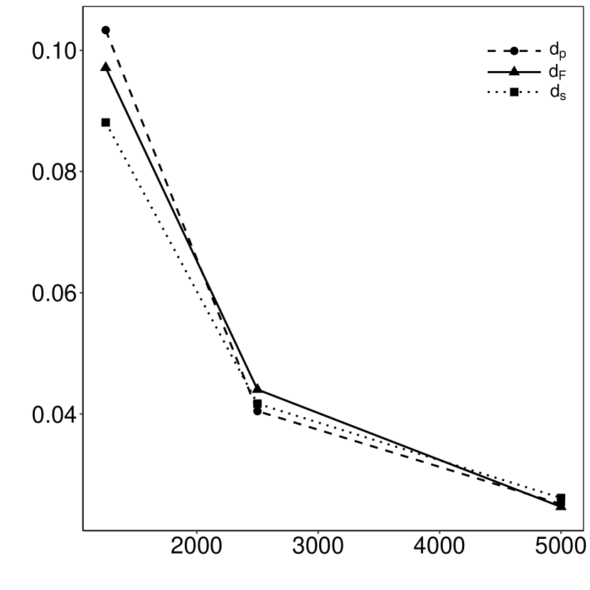
(b) $\mathcal{N}(\boldsymbol{0},{\boldsymbol{\Sigma}_{2}})$

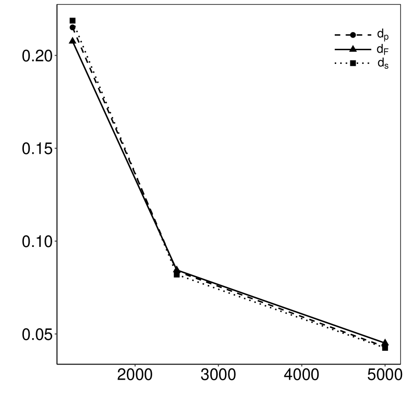
(c) $\mathcal{N}(\boldsymbol{0},{\boldsymbol{\Sigma}_{3}})$

Figure 2: Simulated mean squared error of the parameter estimate in the logistic regression model (2.6) using OBDSS subsamplig with the metric $d_{F}(\cdot)$, $d_{s}(\cdot)$, and $d_{p}(\cdot)$ defined in (3.3), (3.4) and (3.5), respectively. The covariates are normally distributed with different covariance matrices.

4.1.2 Comparison with other subsampling procedures

For the logistic regression model (2.6) there exist several alternative subsampling procedures. Here we consider the IBOSS procedure introduced by Cheng et al., (2020) and a modification of the $mVc$-score-based subsampling developed by Wang et al., (2018), which is called OSMAC. This modification is described below and will always yield an improvement of the original procedure.

In Figure 3 we display the simulated MSE for the different subsampling procedures. We observe that in all cases under consideration, ODBSS has the best performance. It can be seen that the superiority of ODBSS is more pronounced when the size of the subsample is smaller ($k=1250$, which is 1.25% and $k=2500$, which is $2.5\%$ of the original sample size). Moreover, the advantages of ODBSS are more pronounced if the covariates are “concentrating” on a “lower” dimensional space defined by the matrices by ${\boldsymbol{\Sigma}_{2}}$ or ${\boldsymbol{\Sigma}_{3}}$. Interestingly, the mean squared error is smaller for $t$-distributed than for normal distributed predictors.

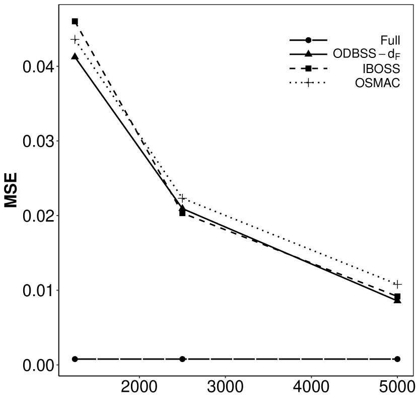
(a) $\mathcal{N}(\boldsymbol{0},{\boldsymbol{\Sigma}_{1}})$

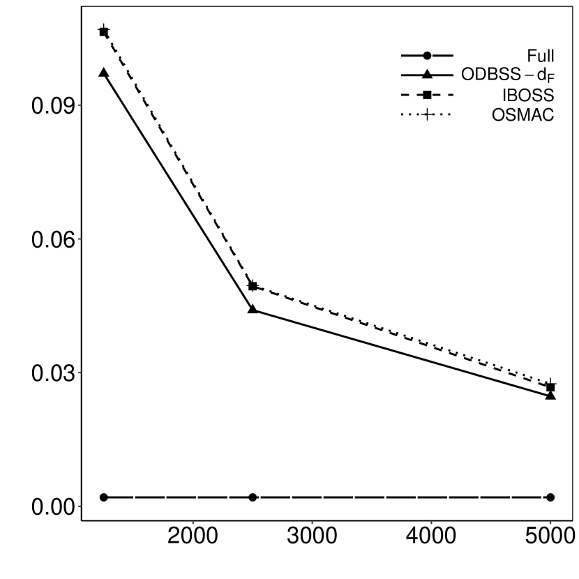
(b) $\mathcal{N}(\boldsymbol{0},{\boldsymbol{\Sigma}_{2}})$

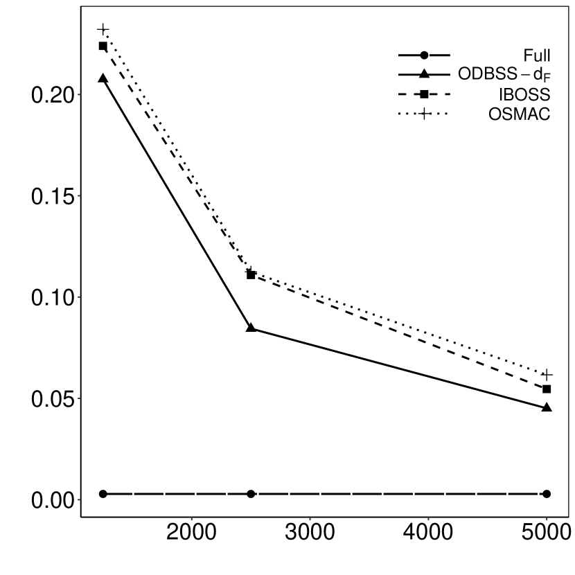
(c) $\mathcal{N}(\boldsymbol{0},{\boldsymbol{\Sigma}_{3}})$

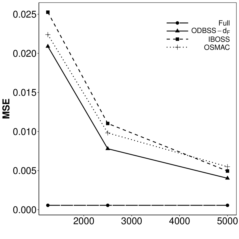
(d) $t_{3}(\boldsymbol{0},{\boldsymbol{\Sigma}_{1}})$

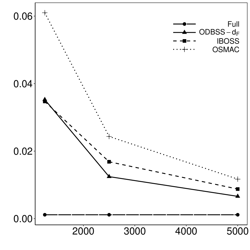
(e) $t_{3}(\boldsymbol{0},{\boldsymbol{\Sigma}_{2}})$

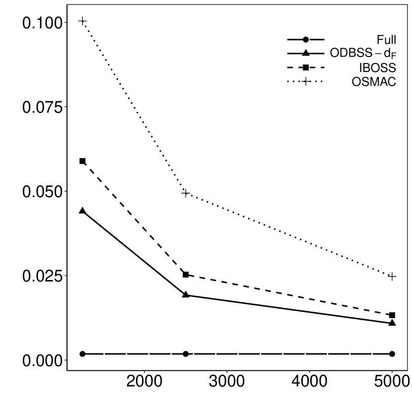
(f) $t_{3}(\boldsymbol{0},{\boldsymbol{\Sigma}_{3}})$

Figure 3: Simulated mean squared error of estimates in the logistic regression model (2.6) based on a subsample obtained by ODBSS, IBOSS, OSMAC, and the full sample. A centered normal and $t$-distribution with $3$ degrees of freedom with different covariance matrices are considered for the predictor.

On the other hand, we do not observe large differences between IBOSS and OSMAC, which partially contradicts the findings in Cheng et al., (2020), who observed substantial advantages of IBOSS over OSMAC. These differences can be explained as follows. The subsample obtained by OSMAC consists of two parts, $k_{0}$ observations obtained by uniform subsampling and $k_{1}=k-k_{0}$ observations obtained by sampling with “optimal” probabilities $\pi_{i}^{mVc}$ (calculated from the initial sample). While Cheng et al., (2020) use OSMAC with the subsample $\mathcal{D}_{k_{1}}$ and weighted maximum likelihood with optimal weights $\pi_{i}^{mVc}$ to estimate the parameters, Wang et al., (2018) use the full sample $\mathcal{D}_{k}$ for this purpose. We argue that both approaches are sub-optimal. On the one hand, using only the sample $\mathcal{D}_{k_{1}}$ does not take all available observations into account. On the other hand, if the full sample $\mathcal{D}_{k}$ is applied for the estimation, the weights $\pi_{i}^{mVc}$ in the likelihood function do not reflect the nature of the random sampling mechanism. In fact, the subsample ${\cal D}_{k}={\cal D}_{k_{0}}\cup{\cal D}_{k_{1}}$ is drawn from a mixture of a uniform and the $\pi^{mVc}$ distribution. Therefore we propose to estimate the parameters from the full subsample ${\cal D}_{k}$ by weighted logistic regression with the weights from the mixture distribution $\widetilde{\pi}_{i}^{mVc}=(k_{0}/k)\leavevmode\nobreak\ (1/n)+(k_{1}/k)\leavevmode\nobreak\ \pi_{i}^{mVc}$ ($i=1,\ldots,n$). This procedure has been implemented in our comparison and we observe that it improves the procedures of Wang et al., (2018) and Cheng et al., (2020) substantially (these results are not displayed for the sake of brevity). In particular, the differences between the two subsampling algorithms are much smaller. Nevertheless, both procedures are outperformed by ODBSS.

4.1.3 Using only the most important points of the optimal design

In Section 3.2, we proposed Algorithm 2, which removes support points of the optimal design with small weights. As this procedure would yield substantial computational advantages of ODBSS it is of interest to investigate its impact on the quality of the estimates based on the resulting subsample. In the left part of Figure 4 we display the simulated mean squared error of the estimator from a subsample obtained by ODBSS, where we apply Algorithm 3 with efficiency thresholds $\zeta=100\%,$ $97.5\%,$ $95\%,$ $90\%,$ and $80\%$ to reduce the number of support points of the optimal design in Step 2 of Algorithm 1. We consider centered normal distributed predictors with covariance matrices $\boldsymbol{\Sigma}_{1}$, $\boldsymbol{\Sigma}_{2}$, and $\boldsymbol{\Sigma}_{3}$. We observe that the MSE increases only very slowly. For example, compared to the normal distribution with covariance matrix $\boldsymbol{\Sigma}_{2}$ the MSE is $0.0279$ if we apply ODBSS using all support points ($100\%$ efficiency) and $0.0257$ if ODBSS uses only the support points of the design with $80\%$ efficiency. In the right panel, we display the corresponding average numbers of support points, which decreases from about 25 to about 10 for all three normal distributions. We observe that the number of support points decreases sharply, as the $A$-efficiency decreases. The designs with $97.5\%$ or $95\%$ $A$-efficiency seem to be a very good choice. In this case, there is not much of an increase in MSE but the computational complexity is reduced to almost half as the number of support points of the optimal design is almost halved at this cutoff.

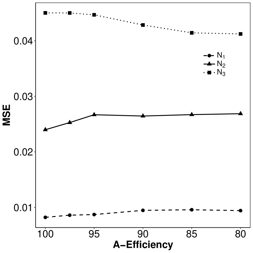
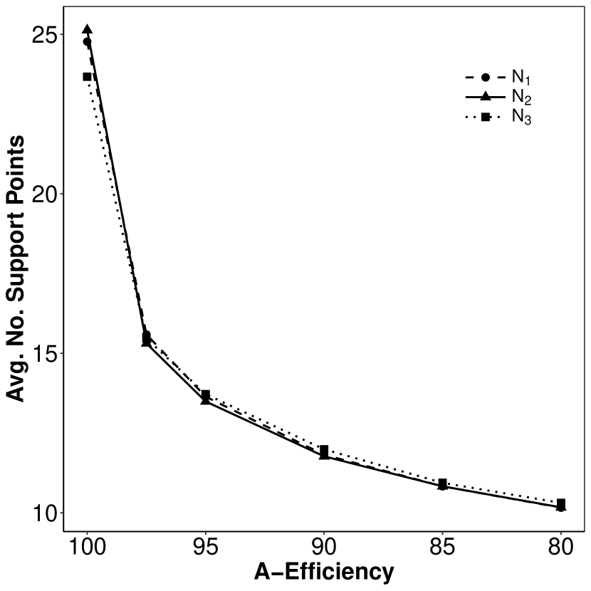
Figure 4: Left: Simulated mean squared of estimates in the logistic regression model (2.6) based on a subsample obtained by ODBSS with a reduced number of support points (see Algorithm 2). Right: average number of support points. The predictor is centered normal distributed with covariance matrices $\boldsymbol{\Sigma}_{1}$ $(N1)$, $\boldsymbol{\Sigma}_{2}$ $(N2)$ and $\boldsymbol{\Sigma}_{3}$ $(N3)$.

4.1.4 Alternative design space estimation

The estimation of the design space proposed in Section 3.1 requires additional computational costs in OBDSS. An obvious alternative here is, to use the full sample $\mathcal{D}$ rather than using a clustering-based area approximation procedure as an approximation for design space, which is required for the calculation of the optimal design in step (2) of Algorithm 1. This will eliminate the area approximation step in step (1) of Algorithm 1 and hence, the time corresponding to this operation. This modification of ODBSS will be denoted by ODBSS-2 in the following discussion. A similar approach was also proposed in Deldossi and Tommasi, (2022). We observe in our numerical studies that the performance of ODBSS and ODBSS-2 is very similar in terms of accuracy for parameter estimation. Exemplary, we display in Figure 5 the mean squared error of parameter estimates in the logistic regression model (2.6) using a subsample obtained from ODBSS and ODBSS-2.

On the other hand, we compare in Table 1 the run times of the two versions of ODBSS for finding a subsample of size $k=5\%\cdot n$. We observe that for $n=100000$ the average run-time of ODBSS-2 is smaller compared to ODBSS. However, as $n$ increases the average run-time of ODBSS-2 sharply increases as $n$ increases, while the changes for ODBSS are rather small. These observations can be explained by taking a closer look at the design space estimation in step (1) and at the optimal design determination in step (2) of Algorithm 1. As only the initial sample subsample $\mathcal{D}_{k_{0}}$ is used in ODBSS for the design space estimation by density-based clustering, the contribution from this step does not increase drastically even if the sample size is increased (the size of the estimated design space ${{\boldsymbol{\chi}}}_{k_{0}}$ does not depend on the sample size rather it depends on the grid size and is at most $L^{p}$, see Section 3.4). On the other hand, ODBSS-2 uses the full sample ${\cal D}$ as an estimate of design space and the number of points in this set is $n$. The differences can be quite substantial. For the example considered above, the number of points of the estimated design space using density-based clustering increases from from $21875$ to $32187$ ($47\%$), if the full sample size increases from $100000$ to $400000$ ($400\%$). As the time complexity for the optimal design determination in step (2) of Algorithm 1 depends on the number of points of the estimated design space (in fact, this is a cubic dependency), the computation time of ODBSS-2 increases sharply with $n$, while it only increases slightly for ODBSS.

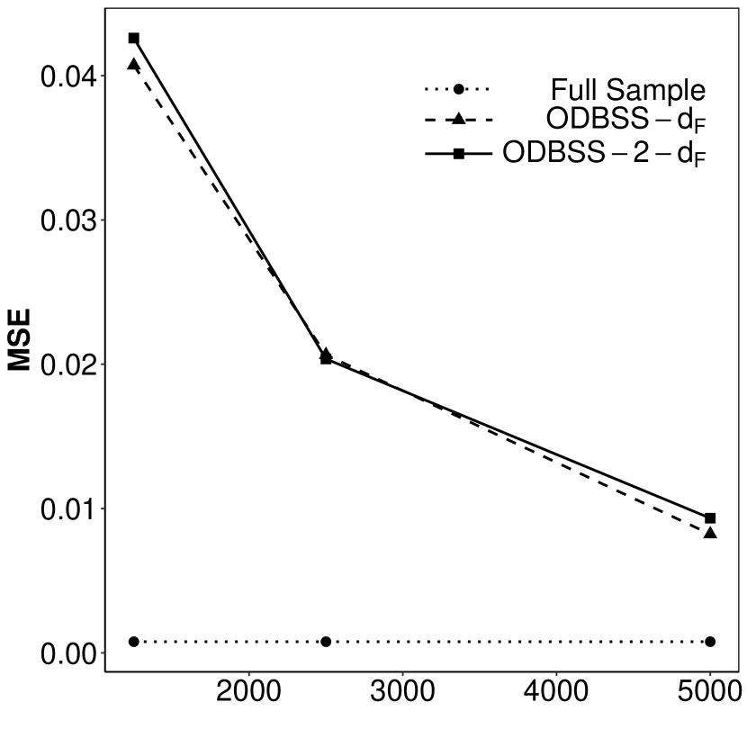
(a) $\mathcal{N}(\boldsymbol{0},{\boldsymbol{\Sigma}_{1}})$

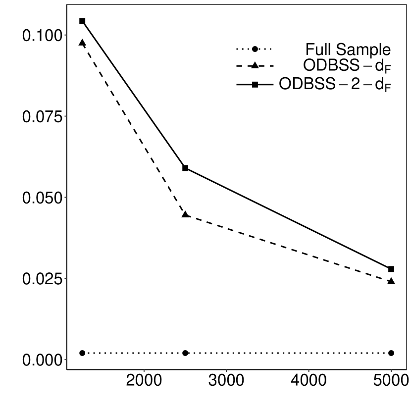
(b) $\mathcal{N}(\boldsymbol{0},{\boldsymbol{\Sigma}_{2}})$

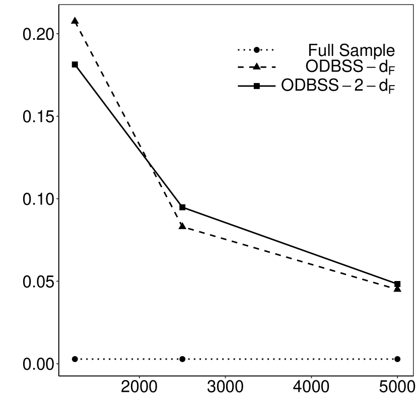
(c) $\mathcal{N}(\boldsymbol{0},{\boldsymbol{\Sigma}_{3}})$

Figure 5: The simulated mean squared error of estimates in the logistic regression model (2.6) based on a subsample obtained by ODBSS and ODBSS-2. A centered normal distribution with different covariance matrices is considered for the predictor.

		$n$
		100000	200000	300000	400000
$\mathcal{N}(\boldsymbol{0},{\boldsymbol{\Sigma}_{1}})$	ODBSS	6.62	8.30	7.78	8.65
	ODBSS-2	5.69	8.76	9.43	13.07
$\mathcal{N}(\boldsymbol{0},{\boldsymbol{\Sigma}_{2}})$	ODBSS	8.21	7.31	8.47	8.04
	ODBSS-2	5.33	8.00	10.85	11.52
$\mathcal{N}(\boldsymbol{0},{\boldsymbol{\Sigma}_{3}})$	ODBSS	5.91	6.26	6.75	9.01
	ODBSS-2	3.87	7.03	9.30	11.22

Table 1: Comparison of the average run-times (seconds) of two versions of Algorithm 1 corresponding to ODBSS and ODBSS-2.

4.2 Heteroskedastic regression - rank $2$ case

So far the literature subsampling strategies consider models where the rank of the Fisher information matrix is $1$. In this section, we demonstrate that Algorithm 1 can also deal with more general cases without any modification. Consider the model in Example 2.3, where the variance is a deterministic function of the expectation, that is

$$g(\boldsymbol{x},\boldsymbol{\beta}) =\boldsymbol{z}^{\top}\boldsymbol{\beta}\leavevmode\nobreak\ ,$$ (4.2)

$$\sigma^{2}({\boldsymbol{x},\boldsymbol{\beta}}) =\exp{(\boldsymbol{x}^{\top}(\beta_{1},\dots,\beta_{p})^{\top})}.$$ (4.3)

In this model, the maximum likelihood estimator is defined by

$$\hat{\boldsymbol{\beta}}=\arg\max_{\boldsymbol{\beta}}\Big{\{}-\dfrac{n}{2}\log(2\pi)-\dfrac{1}{2}\sum_{i=1}^{n}\log\sigma^{2}(\boldsymbol{x}_{i},\boldsymbol{\beta})-\dfrac{1}{2}\sum_{i=1}^{n}\dfrac{(y_{i}-\boldsymbol{z}_{i}^{\top}\boldsymbol{\beta})^{2}}{\sigma^{2}(\boldsymbol{x}_{i},\boldsymbol{\beta})}\Big{\}}.$$ (4.4)

The Fisher-information matrix at point $\boldsymbol{x}$ is given by

$$\mathcal{I}(\beta,\boldsymbol{x})=\dfrac{1}{\sigma^{2}({\boldsymbol{x},\boldsymbol{\beta}})}\begin{pmatrix}1\\ \boldsymbol{x}\end{pmatrix}\leavevmode\nobreak\ (1\leavevmode\nobreak\ \leavevmode\nobreak\ \leavevmode\nobreak\ \boldsymbol{x})+\dfrac{1}{2}\begin{pmatrix}0\\ \boldsymbol{x}\end{pmatrix}\leavevmode\nobreak\ (0\leavevmode\nobreak\ \leavevmode\nobreak\ \leavevmode\nobreak\ \boldsymbol{x})$$

and has rank equal $2$ if $\boldsymbol{x}\not=0$. We investigate the performance of ODBSS (Algorithm 1) for finding the most informative subsamples. In the simulation experiment, we consider the case $p=7$ and the parameter $\boldsymbol{\beta}=(0.25,\ldots,0.25)^{\top}$ and three setups: covariates are generated from a normal distribution with the three different covariance matrices from Section 4.1.1. The sample size is fixed at $n=100000$ and the subsample sizes are varied from $k=5000,2500,1250$. As expected, the ODBSS is much better than the uniform random subsampling.

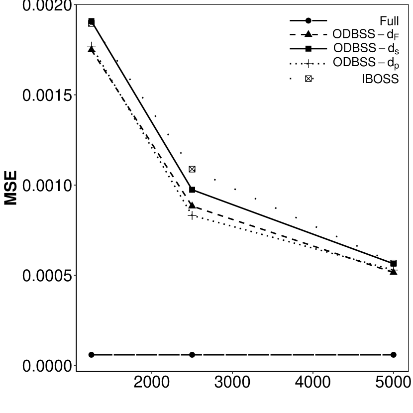
(a) $\mathcal{N}(\boldsymbol{0},{\boldsymbol{\Sigma}_{1}})$

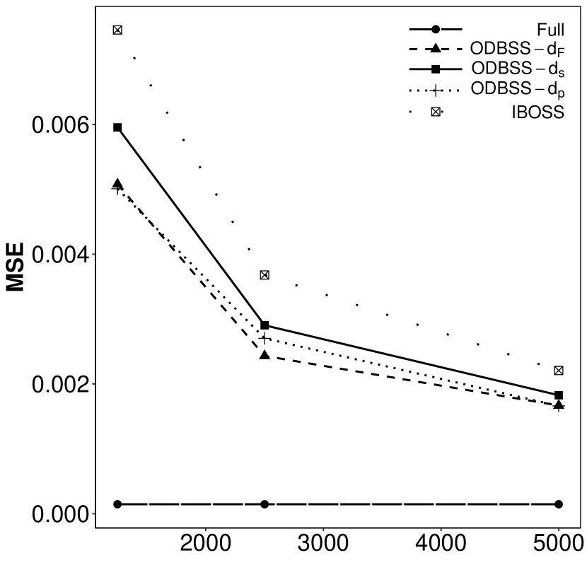
(b) $\mathcal{N}(\boldsymbol{0},{\boldsymbol{\Sigma}_{2}})$

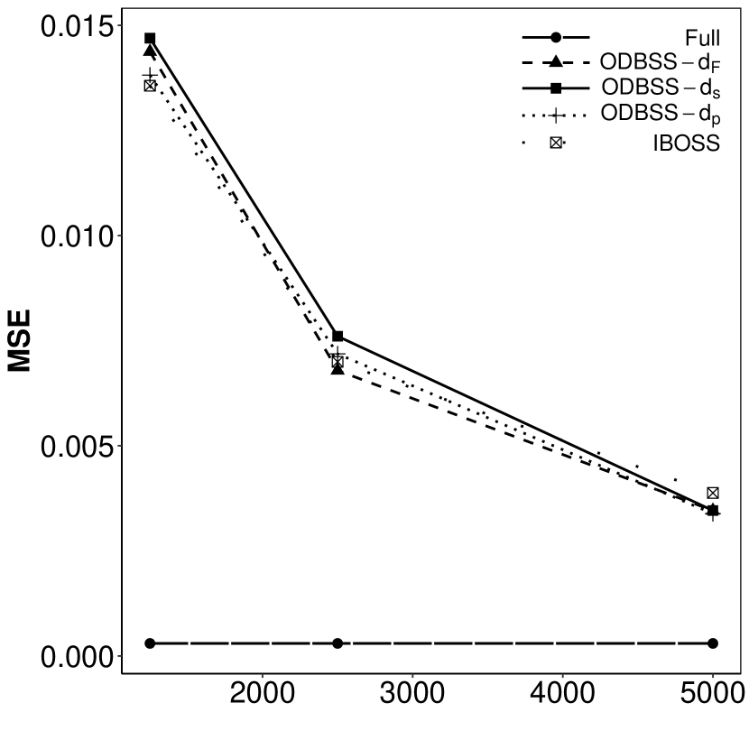
(c) $\mathcal{N}(\boldsymbol{0},{\boldsymbol{\Sigma}_{3}})$

Figure 6: Simulated mean squared error of the parameter estimate in the heteroskedastic regression model given by equation (4.2) and (4.3) using OBDSS subsampling with the metric $d_{F}(\cdot)$, $d_{s}(\cdot)$, and $d_{p}(\cdot)$ defined in (3.3), (3.4) and (3.5), respectively. A comparison of ODBSS (all three distances) with an IBOSS subsample. The covariates are normally distributed with different covariance matrices (as in section 4.1).

From Figure 6, we observe that all three matrix distances yield a very comparable performance of ODBSS. Using ODBSS with the Procrustes and Frobenius metric gives slightly better results than with square root distance. For the sake of comparison we have also included the results of IBOSS as proposed by Wang et al., (2019). We observe that in most cases ODBSS has a better performance than IBOSS as well. Its superiority is more pronounced on the subspaces defined by covariance matrices $\Sigma_{1}$ and $\Sigma_{2}$.

5 Concluding remarks and future research

In this paper, we develop a new deterministic subsampling strategy, which is applicable for finding maximum likelihood estimates for a large class of models. Subsampling is carried out in three steps: i) design space estimation from a small initial sample, ii) the optimal design determination for the estimated design space, and iii) subsample allocation. Simulation experiments show an improved performance of the new method over competing algorithms. The structure of the algorithm allows to modify it for an online subsampling setting easily. For this setup step i) and ii), which determines the optimal design could be used adaptively (in batches) to determine subsamples that should be retained (depending upon proximity to the optimal design). These extensions will be investigated in future research. A further interesting question is statistical guarantees for the estimates based on the sample of the proposed algorithm.

Software used for computation. We have implemented the ODBSS algorithm for the simulation studies in $R$-software(R-4.2.0) and MATLAB-R2022.

Acknowledgements. This work was partially supported by the DFG Research unit 5381 Mathematical Statistics in the Information Age, project number 460867398.

References

- Ai et al., (2021) Ai, M., Wang, F., Yu, J., and Zhang, H. (2021). Optimal subsampling for large-scale quantile regression. Journal of Complexity, 62:101512.
- Atkinson and Cook, (1995) Atkinson, A. C. and Cook, R. D. (1995). D-optimum designs for heteroscedastic linear models. Journal of the American Statistical Association, 90(429):204–212.
- Ben-Tal and Nemirovski, (2001) Ben-Tal, A. and Nemirovski, A. (2001). Lectures on modern convex optimization: analysis, algorithms, and engineering applications. SIAM.
- Cheng et al., (2020) Cheng, Q., Wang, H., and Yang, M. (2020). Information-based optimal subdata selection for big data logistic regression. Journal of Statistical Planning and Inference, 209:112–122.
- Deldossi and Tommasi, (2022) Deldossi, L. and Tommasi, C. (2022). Optimal design subsampling from big datasets. Journal of Quality Technology, 54(1):93–101.
- Dette and Holland-Letz, (2009) Dette, H. and Holland-Letz, T. (2009). A geometric characterization of c-optimal designs for heteroscedastic regression. The Annals of Statistics, pages 4088–4103.
- Dryden et al., (2009) Dryden, I. L., Koloydenko, A., and Zhou, D. (2009). Non-Euclidean statistics for covariance matrices, with applications to diffusion tensor imaging. The Annals of Applied Statistics, 3(3):1102 – 1123.
- Ester et al., (1996) Ester, M., Kriegel, H.-P., Sander, J., Xu, X., et al. (1996). A density-based algorithm for discovering clusters in large spatial databases with noise. In kdd, volume 96, pages 226–231.
- Hahsler et al., (2022) Hahsler, M., Piekenbrock, M., Arya, S., and Mount, D. (2022). dbscan: Density-Based Spatial Clustering of Applications with Noise (DBSCAN) and Related Algorithms. R package version 1.1-11.
- Harman and Lenka, (2019) Harman, R. and Lenka, F. (2019). OptimalDesign: A Toolbox for Computing Efficient Designs of Experiments. R package version 1.0.1.
- Kiefer, (1974) Kiefer, J. (1974). General equivalence theory for optimum designs (approximate theory). The Annals of Statistics, 2:849–879.
- Lehmann and Casella, (2006) Lehmann, E. L. and Casella, G. (2006). Theory of point estimation. Springer Science & Business Media.
- Ma et al., (2015) Ma, P., Mahoney, M., and Yu, B. (2015). A statistical perspective on algorithmic leveraging. Journal of Machine Learning Research, 16(27):861–911.
- Martınez, (2004) Martınez, C. (2004). Partial quicksort. In Proc. 6th ACMSIAM Workshop on Algorithm Engineering and Experiments and 1st ACM-SIAM Workshop on Analytic Algorithmics and Combinatorics, pages 224–228.
- Pigoli et al., (2014) Pigoli, D., Aston, J. A., Dryden, I. L., and Secchi, P. (2014). Distances and inference for covariance operators. Biometrika, 101(2):409–422.
- Pukelsheim, (2006) Pukelsheim, F. (2006). Optimal Design of Experiments. SIAM, Philadelphia.
- Randall et al., (2007) Randall, T., Donev, A., and Atkinson, A. (2007). Optimum Experimental Designs, with SAS. Oxford University Press.
- Ren and Zhao, (2021) Ren, M. and Zhao, S.-L. (2021). Subdata selection based on orthogonal array for big data. Communications in Statistics-Theory and Methods, pages 1–19.
- Sagnol and Harman, (2015) Sagnol, G. and Harman, R. (2015). Computing exact d-optimal designs by mixed integer second-order cone programming. The Annals of Statistics, 43(5):2198–2224.
- Schubert et al., (2017) Schubert, E., Sander, J., Ester, M., Kriegel, H. P., and Xu, X. (2017). Dbscan revisited, revisited: why and how you should (still) use dbscan. ACM Transactions on Database Systems (TODS), 42(3):1–21.
- Silvey, (1980) Silvey, S. (1980). Optimal design: an introduction to the theory for parameter estimation, volume 1. Chapman and Hall.
- Wang, (2019) Wang, H. (2019). More efficient estimation for logistic regression with optimal subsamples. Journal of machine learning research, 20.
- Wang and Ma, (2020) Wang, H. and Ma, Y. (2020). Optimal subsampling for quantile regression in big data. Biometrika, 108(1):99–112.
- Wang et al., (2019) Wang, H., Yang, M., and Stufken, J. (2019). Information-based optimal subdata selection for big data linear regression. Journal of the American Statistical Association, 114(525):393–405.
- Wang et al., (2018) Wang, H., Zhu, R., and Ma, P. (2018). Optimal subsampling for large sample logistic regression. Journal of the American Statistical Association, 113(522):829–844.
- Wang et al., (2021) Wang, L., Elmstedt, J., Wong, W. K., and Xu, H. (2021). Orthogonal subsampling for big data linear regression. The Annals of Applied Statistics, 15(3):1273–1290.
- Yao and Wang, (2021) Yao, Y. and Wang, H. (2021). A review on optimal subsampling methods for massive datasets. Journal of Data Science, 19(1):151–172.
- Yu et al., (2022) Yu, J., Wang, H., Ai, M., and Zhang, H. (2022). Optimal distributed subsampling for maximum quasi-likelihood estimators with massive data. Journal of the American Statistical Association, 117(537):265–276.