Zero-temperature stochastic Ising model on planar quasi-transitive graphs

Abstract.

We study the zero-temperature stochastic Ising model on some connected planar quasi-transitive graphs, which are invariant under rotations and translations. The initial spin configuration is distributed according to a Bernoulli product measure with parameter $p\in(0,1)$. In particular, we prove that if $p=1/2$ and the graph underlying the model satisfies the planar shrink property then all vertices flip infinitely often almost surely.

Keywords: Coarsening; zero-temperature dynamics; quasi-transitive planar graphs.

AMS MSC 2010: 82C20, 82C35.

1. Introduction

In this paper, we deal with the zero-temperature stochastic Ising model $(\sigma_{t})_{t\geq 0}$ on some connected planar quasi-transitive graphs with homogeneous ferromagnetic interactions (see e.g. [17, 27]), i.e. all the interactions are equal to a positive constant. The initial spin configuration is distributed according to a Bernoulli product measure with parameter $p\in(0,1)$, see e.g. [16, 26, 27]. The dynamic evolves in the following way: each vertex, at rate $1$, changes its spin value if it disagrees with the majority of its neighbours and determines its spin value by a fair coin toss in case of a tie between the spins of its neighbours. This process is often referred to as domain coarsening or majority dynamics and it is sometimes used as an opinion model.

A question of particular relevance is whether for each vertex $v$ its spin flips only finitely many times almost surely, i.e. in other words whether $\sigma_{t}$ has an almost sure limit. We say that a vertex $v$ fixates if the spin at $v$ flips only finitely many times. According to the classification given in [17], a model is of type $\mathcal{I}$ if no site fixates almost surely, i.e all sites flip infinitely often a.s.; a model is of type $\mathcal{F}$ if all sites fixate almost surely, i.e. all sites flip only finitely many times a.s. and it is said of type ${\mathcal{M}}$ if there are both vertices that fixate and vertices that do not fixate almost surely.

The literature in the early years focused on the cubic lattice $\mathbb{Z}^{d}$ and mainly with $d=2$. It is known that the zero-temperature stochastic Ising model on $\mathbb{Z}$ with homogeneous ferromagnetic interactions is of type $\mathcal{I}$ for any initial density $p\in(0,1)$ (see [1, 27]).

The disordered model on $\mathbb{Z}^{d}$, if the interactions $\{J_{x,y}\}$ are independent random variables with continuous distribution, is of type $\mathcal{F}$ (see [13, 27]). Moreover, in $d=2$ the homogeneous ferromagnetic model is of type $\mathcal{I}$ (see [27]). In [17], an analysis of the zero-temperature stochastic Ising model on $\mathbb{Z}^{d}$ with nearest-neighbour interactions distributed according to a measure $\mu_{J}$ (disordered model) is performed. In particular, it is proved that if the interactions are i.i.d. taking only the values $\pm J$ then the two dimensional model is of type ${\mathcal{M}}$. An analogous result for $d>2$ with a temperature fast decreasing to zero is obtained in [7]. On the cubic lattice $\mathbb{Z}^{d}$, if initial configuration is distributed according to a Bernoulli product measure with parameter $p$ sufficiently close to $1$ (i.e. if $p>p^{\star}_{d}$), then the model is of type $\mathcal{F}$, in particular each vertex fixates at the value $+1$ (see [16]). Moreover in [26] it is shown that $p^{\star}_{d}\to 1/2$ as $d\to\infty$. For homogeneous trees of degree at least $3$ and $p$ sufficiently close to $1$, it has been shown that the model is of type $\mathcal{F}$ (see [6, 15]).

In [9, 11], the case in which one or infinitely many vertices are frozen is studied. The main result of the first paper is that for $d=2$ the model, with infinitely many frozen vertices, is of type $\mathcal{F}$. On the contrary, in the second paper the authors show that the model in $d=2$ is of type $\mathcal{I}$ when only one spin is frozen.

For articles on the stochastic Ising model on graphs other than $\mathbb{Z}^{d}$ see for example [5, 7, 8, 10, 12, 18, 19]; in particular in [5] it is shown that the zero-temperature Ising model on the hexagonal lattice is of type $\mathcal{F}$ and in [7] it is proved that it is not of type $\mathcal{F}$ if simultaneous spin flips are allowed. In [18] the authors studied the Dilute Curie–Weiss Model, i.e. the Ising Model on a dense Erdős-Rényi random graph, and proved that depending on the distribution of interactions there are different behaviors.

In this paper, we deal with connected planar quasi-transitive graphs. The quasi-transivity of the graph will be given by the invariance under translations and rotations. We will show that, under mild assumptions, the only rotations to consider are those of an angle $\theta\in\left\{\frac{\pi}{3},\frac{\pi}{2},\frac{2}{3}\pi,\pi\right\}$ (see Lemma 3 and Theorem 1). Such a class of graphs includes, for instance, the square, the triangular and the hexagonal lattice.

Our first result on the zero-temperature stochastic Ising model (Theorem 2) shows that a necessary condition for the model to be of type $\mathcal{I}$ is that the underlying graph has the shrink property. For example, the hexagonal lattice does not have the shrink property and the model on this lattice is of type $\mathcal{F}$ (see [27]). Thus, we will focus on a class of graphs having the shrink property. Actually, for technical reasons, we will use a potentially stronger definition of the shrink property that is the planar shrink property.

Our main result (Theorem 4) shows that if $p=1/2$ and the graph is invariant under rotations, translations and has the planar shrink property, then the model is of type $\mathcal{I}$.

Here we briefly present the general strategy to prove this achievement. First we show two preliminary results on general attractive spin systems with initial density $p\in(0,1]$ (see Lemmas 1-2). More precisely we show that, for an attractive system, if a spin fixates to $+1$ with positive probability then the probability that it is constantly equal to $+1$ for all times $t\in[0,\infty)$ is positive. After the general analysis developed in Theorems 1-2 we specifically study the zero-temperature stochastic Ising model. First we show that, under the shrink property and the translation-ergodicity, the cardinality of any cluster grows to infinity almost surely (Theorem 3). By this preliminary result, we are able to show that the cluster at the origin will intersect the boundary of any finite region infinitely often for $t\in[0,\infty)$ with probability one. As already mentioned, we consider a planar graph that is invariant under translations and rotations of $\theta\in\left\{\frac{\pi}{3},\frac{\pi}{2},\frac{2}{3}\pi\right\}$. Then, we construct a planar regular region centered at the origin that has the same rotation invariance of the graph. By the FKG inequality and the rotation invariance of the region, the cluster in the origin will intersect all the sides of the regular region with a positive probability larger or equal to $p_{cross}$. We stress that, for $t$ growing to infinity, the quantity $p_{cross}$ does not depend on the size of the region. By these properties and by the previous results we show that any ball centered in the origin has its spins equal to $+1$ infinitely often with a probability larger of $p_{cross}$ (see Lemmas 5-9). Thus, with probability at least $p_{cross}$ no site will be able to fixate at the value $-1$. Finally, by considering the initial density $p=1/2$ and by Lemmas 2-9, we show that all sites flip infinitely often almost surely (see Theorem 4).

The plan of the paper is the following. In Section 2, we define the zero-temperature stochastic Ising model, introduce the underlying graph and present some general results on attractive systems that will be useful for our discussion (see Lemmas 1-3 and Theorem 1). In Section 3, the main result, Theorem 4, is stated and proved through some lemmas and theorems. In Section 4, we present an infinite class of graphs having the planar shrink property (see Theorem 5). We also provide examples of graphs that have and do not have the shrink property, cases where the Ising model is of type $\mathcal{I}$ in the first case, and of type either $\mathcal{M}$ or $\mathcal{F}$, in the latter.

2. Preliminaries

In this section, we introduce the graph underlying the zero-temperature stochastic Ising model and present some preliminary results that will be useful for our discussion in the next section. In particular, in Subsection 2.1 we define the Markov process by the infinitesimal generator and by the Harris’ graphical representation. Moreover, we state two general lemmas (Lemma 1 and Lemma 2) for Glauber attractive dynamics. In Subsection 2.2, we introduce some notation on graphs and define the collection of graphs in which we are interested. More precisely we present in Lemma 3 and Theorem 1 some properties of sets in $\mathbb{R}^{2}$ that are translation and rotation invariant. In Subsection 2.3, we describe in detail the zero-temperature stochastic Ising model $I(G,p)$, where $G$ is the underlying graph and $p$ is the initial density. Moreover, we prove Theorem 2, which shows that the shrink property is a necessary condition to obtain that the $I(G,p)$-model is of type $\mathcal{I}$.

2.1. Attractive spin systems

We now introduce the spin systems referring mainly to [24, Chapter 3]. We consider a spin system $(\sigma_{t})_{t\geq 0}$, which describes $\pm 1$ spin flips dynamics on a countable set of vertices $V$. The state space is $\Sigma=\{+1,-1\}^{V}$. The value of the spin at vertex $v\in V$ at time $t$ will be denoted by $\sigma_{t}(v)$. We introduce the usual order relation $\leq$ on $\Sigma$: given two configurations $\sigma,\sigma^{\prime}\in\Sigma$, we say that $\sigma\leq\sigma^{\prime}$ if for each $v\in V$, $\sigma(v)\leq\sigma^{\prime}(v)$. The spin system $(\sigma_{t})_{t\geq 0}$ evolves as a Markov process on the state space $\Sigma$ with infinitesimal generator $L_{t}$, which acts on local functions $f$, and defined as

$$(L_{t}f)(\sigma)=\sum_{v\in V}c_{t}(v,\sigma)\bigl{(}f(\sigma^{v})-f(\sigma)\bigr{)},$$ (1)

where $t\geq 0$, $c_{t}(v,\sigma)$ is the flip rate of the spin at vertex $v$, and $\sigma^{v}\in\Sigma$ is defined in the following way:

$$\sigma^{v}(u)=\begin{cases}\sigma(u)&\text{if $u\neq v$}\\ -\sigma(u)&\text{if $u=v$}.\end{cases}$$

We assume that $c_{t}(v,\sigma)$ is a uniformly bounded non-negative function, which is continuous on $\sigma$ and satisfies the condition

$$\sup_{v\in V}\sum_{w\in V}\sup_{\sigma\in\Sigma}|c_{t}(v,\sigma)-c_{t}(v,\sigma^{w})|<\infty.$$ (2)

The condition in (2) guarantees the existence of the Markov process with infinitesimal generator $L_{t}$ (see [24]). We take the process $(\sigma_{t})_{t\geq 0}$ right continuous.

We say that a spin system is attractive if $c_{t}(v,\sigma)$ is increasing in $\sigma$ when $\sigma(v)=-1$ and decreasing in $\sigma$ when $\sigma(v)=+1$. We are in particular interested to study Glauber dynamics, for which the relation

$$c_{t}(v,\sigma)=1-c_{t}(v,\sigma^{v})$$ (3)

holds for each $v\in V$, $\sigma\in\Sigma$ and $t\geq 0$. If the relation (3) holds, then $0\leq c_{t}(v,\sigma)\leq 1$. We write the flip rates in the form

$$c_{t}(v,\sigma)=\tilde{c}_{t}(v,(\sigma(u))_{u\in A_{v}}),$$ (4)

where $A_{v}$ is a subset of $V$. Under (3) and the assumption

$$\sup_{v\in V}|A_{v}|<\infty,$$ (5)

the process defined in (1) can be constructed by the Harris’ graphical representation (see e.g. [20, 22, 23, 24]), which we now describe. We consider a collection $({\mathcal{P}}_{v})_{v\in V}$ of independent Poisson processes with rate $1$ interpreted as counting processes. For each $v\in V$, let ${\mathcal{T}}_{v}=(\tau_{v,n}:n\in\mathbb{N})$ be the ordered sequence of arrivals of the Poisson process ${\mathcal{P}}_{v}$, associated with the vertex $v$. The probability that there is a flip at vertex $v$ at time $t$ (conditioning on the event $\{t\in{\mathcal{T}}_{v}\}$) is equal to $c_{t}(v,\sigma_{t^{-}})$, where $\sigma_{t^{-}}:=\lim_{s\to t^{-}}\sigma_{s}$. For convenience, to describe these events in more detail, we can use a family of i.i.d. random variables $(U_{v,n}:v\in V,n\in\mathbb{N})$ distributed according to a uniform random variable in $[0,1]$ and such that if $U_{v,n}<c_{\tau_{v,n}}(v,\sigma_{\tau_{v,n}^{-}})$, then the spin at $v$ flips at time $\tau_{v,n}$ (see [22] and [24]).

Lemma 1 below is well known, but we present a proof in order to construct the coupling that will be used in the proof of Lemma 2.

Lemma 1.

Given two Glauber attractive dynamics $(\sigma_{t})_{t\geq 0}$ and $(\sigma^{\prime}_{t})_{t\geq 0}$ having the same generator and such that $\sigma_{0}\leq\sigma^{\prime}_{0}$, there exists a coupling such that $\sigma_{t}\leq\sigma^{\prime}_{t}$ for each $t\geq 0$.

Proof.

By hypothesis the order relation is satisfied at the initial time. Hence, it is sufficient to consider a single arrival of the Poisson process, i.e. only a possible spin flip, in order to show that the order relation is maintained, i.e. we will show that $\sigma_{\tau_{v,n}^{-}}(v)=+1>\sigma^{\prime}_{\tau_{v,n}^{-}}(v)=-1$ does not occur.

Let us explicitly construct the desired coulping. We use the same Poisson processes for the two systems, but different families of i.i.d. uniform random variables $(U_{v,n}:v\in V,n\in\mathbb{N})$ and $(U^{\prime}_{v,n}:v\in V,n\in\mathbb{N})$ for $(\sigma_{t})_{t\geq 0}$ and $(\sigma^{\prime}_{t})_{t\geq 0}$ respectively.

For each $v,v^{\prime}\in V$ and $n\in\mathbb{N}$, let us consider the stopping time $\tau_{v,n}$. Moreover, for $v^{\prime}\in V\setminus\{v\}$ let us define

$$N(n,v,v^{\prime}):=\sup\{\ell\in\mathbb{N}:\tau_{v^{\prime},\ell}\leq\tau_{v,n}\}.$$

We notice that $N(n,v,v)=n$, moreover for $v^{\prime}\neq v$ one has $\tau_{v^{\prime},N(n,v,v^{\prime})}<\tau_{v,n}$ almost surely.

If $\sigma_{\tau_{v,n}^{-}}(v)=\sigma^{\prime}_{\tau^{-}_{v,n}}(v)$ then we define $U^{\prime}_{v,n}=U_{v,n}$, if $\sigma_{\tau_{v,n}^{-}}(v)=-1<\sigma^{\prime}_{\tau_{v,n}^{-}}(v)=+1$ then we define $U^{\prime}_{v,n}=1-U_{v,n}$. Hence, the random variable $U^{\prime}_{v,n}$ is a function of

$$(U_{v,1},\ldots,U_{v,n-1})$$ (6)

and of the independent sequences $(U_{v^{\prime},\ell}:v^{\prime}\in V\setminus\{v\},\ell\leq N(n,v,v^{\prime}))$ and $(\mathcal{P}_{v^{\prime}}(t):v^{\prime}\in V,t\leq\tau_{v,n})$.

If $U^{\prime}_{v,n}=U_{v,n}$, by construction, $U^{\prime}_{v,n}$ is independent from $U^{\prime}_{v,1},\dots,U^{\prime}_{v,n-1}$, which altogether are functions of $U_{v,1},\dots,U_{v,n-2}$, of $\{U_{v^{\prime},\ell}:v^{\prime}\in V\setminus\{v\},\ell\leq N(n-1,v,v^{\prime})\}$ and $(\mathcal{P}_{v^{\prime}}(t):v^{\prime}\in V,t\leq\tau_{v,n-1})$. Otherwise, if $U^{\prime}_{v,n}=1-U_{v,n}$ independence follows by:

$${\mathbb{P}}(U^{\prime}_{v,n}\in[a,b]|U_{v,1}=u_{1},\dots,U_{v,n-1}=u_{n-1})=\\ ={\mathbb{P}}(U_{v,n}\in[1-b,1-a]|U_{v,1}=u_{1},\dots,U_{v,n-1}=u_{n-1})=\\ ={\mathbb{P}}(U_{v,n}\in[1-b,1-a])=b-a={\mathbb{P}}(U^{\prime}_{v,n}\in[a,b]),$$

where $0<a<b<1$ and $u_{1},\ldots u_{n-1}\in(0,1)$. This implies that the distribution of $U^{\prime}_{v,n}$ and the conditional distribution of $U^{\prime}_{v,n}$ given $U^{\prime}_{v,1},\dots,U^{\prime}_{v,n-1}$ coincide, hence $U^{\prime}_{v,n}$ is independent from $U^{\prime}_{v,1},\dots,U^{\prime}_{v,n-1}$ and $U^{\prime}_{v,n}$ is a uniform random variable on $[0,1]$. The independence of different sequences of uniform random variables can be proved in a similar way.

Whenever there is an arrival of a Poisson process, for example at time $t$ for the vertex $v$ (i.e. $t\in{\mathcal{T}}_{v}\$), the following situations can arise:

Case $\sigma_{\tau_{v,n}^{-}}(v)=\sigma^{\prime}_{\tau_{v,n}^{-}}(v)=-1$.
Since $U_{v,n}=U^{\prime}_{v,n}$ and $c_{\tau_{v,n}}(v,\sigma_{\tau_{v,n}^{-}})$ is increasing in $\sigma$, we have the following three situations: if $U_{v,n}<c_{\tau_{v,n}}(v,\sigma_{\tau_{v,n}^{-}})\leq c_{\tau_{v,n}}(v,\sigma^{\prime}_{\tau_{v,n}^{-}})$ then both systems change the spin value at $v$; if $c_{\tau_{v,n}}(v,\sigma_{\tau_{v,n}^{-}})\leq U_{v,n}<c_{\tau_{v,n}}(v,\sigma^{\prime}_{\tau_{v,n}^{-}})$ then in the system $(\sigma_{t})_{t\geq 0}$ the spin at $v$ does not change its value, while in $(\sigma^{\prime}_{t})_{t\geq 0}$ the spin flip occurs at $v$; if $c_{\tau_{v,n}}(v,\sigma_{\tau_{v,n}^{-}})\leq c_{\tau_{v,n}}(v,\sigma^{\prime}_{\tau_{v,n}^{-}})\leq U_{v,n}$ then both systems do not have the spin flip at $v$. In all these three situations the order relation is maintained.

Case $\sigma_{\tau_{v,n}^{-}}(v)=\sigma^{\prime}_{\tau_{v,n}^{-}}(v)=+1$.
Since $U_{v,n}=U^{\prime}_{v,n}$ and $c_{\tau_{v,n}}(v,\sigma_{\tau_{v,n}^{-}})$ is decreasing in $\sigma$, we have the following three situations: if $U_{v,n}<c_{\tau_{v,n}}(v,\sigma^{\prime}_{\tau_{v,n}^{-}})\leq c_{\tau_{v,n}}(v,\sigma_{\tau_{v,n}^{-}})$ then both systems change the spin value at $v$; if $c_{\tau_{v,n}}(v,\sigma^{\prime}_{\tau_{v,n}^{-}})\leq U_{v,n}<c_{\tau_{v,n}}(v,\sigma_{\tau_{v,n}^{-}})$ then in the system $(\sigma_{t})_{t\geq 0}$ the spin at $v$ change its value, while in $(\sigma^{\prime}_{t})_{t\geq 0}$ the spin flip does not occur at $v$; if $c_{\tau_{v,n}}(v,\sigma^{\prime}_{\tau_{v,n}^{-}})\leq c_{\tau_{v,n}}(v,\sigma_{\tau_{v,n}^{-}})\leq U_{v,n}$ then both systems do not have the spin flip at $v$. In all these three situations the order relation is maintained.

Case $\sigma_{\tau_{v,n}^{-}}(v)=-1<\sigma^{\prime}_{\tau_{v,n}^{-}}(v)=+1$.
If $U_{v,n}<c_{\tau_{v,n}}(v,\sigma_{\tau_{v,n}^{-}})$ then, since in this case $U^{\prime}_{v,n}=1-U_{v,n}$, by using the relation (3) for Glauber dynamics and by attractivity, one has that

$$U^{\prime}_{v,n}=1-U_{v,n}>1-c_{\tau_{v,n}}(v,\sigma_{\tau_{v,n}^{-}})=c_{\tau_{v,n}}(v,\sigma^{v}_{\tau_{v,n}^{-}})\geq c_{\tau_{v,n}}(v,\sigma^{\prime}_{\tau_{v,n}^{-}}).$$

Thus, in the system $(\sigma_{t})_{t\geq 0}$ the spin at $v$ changes its value, while in $(\sigma^{\prime}_{t})_{t\geq 0}$ the spin flip does not occur at $v$, maintaining the order relation. If $U_{v,n}\geq c_{\tau_{v,n}}(v,\sigma_{\tau_{v,n}^{-}})$, the spin at $v$ in $(\sigma_{t})_{t\geq 0}$ does not change and therefore the order relation is maintained.

By previous cases and since $\sigma_{0}\leq\sigma^{\prime}_{0}$, one deduces that the order relation is maintained at any time. Hence $\sigma_{\tau_{v,n}^{-}}(v)=+1$ and $\sigma^{\prime}_{\tau_{v,n}^{-}}(v)=-1$ does not occur. ∎

Now, we give the following definition which will be used in the next Lemma 2.

Definition 1.

We say that a vertex $v$ fixates if the spin at $v$ flips only finitely many times and we say that a vertex fixates from time zero if its spin never flips.

In the following Lemma 2, for Glauber attractive systems, we compare the probability that a spin fixates or fixates from time zero.

Lemma 2.

Consider a Glauber attractive dynamics $(\sigma_{t})_{t\geq 0}$ where $\sigma_{0}$ has density $p\in(0,1]$. If a vertex $w$ fixates at the value $+1$ with positive probability, then the vertex $w$ fixates at the value $+1$ from time zero with positive probability.

Proof.

We define $T_{w}:=\inf\{s\geq 0:\sigma_{t}(w)=+1\ \ \forall t\geq s\}$, where $\inf\emptyset=+\infty$. We assume that ${\mathbb{P}}(T_{w}<\infty)=\rho>0$ and we choose $\bar{t}$ such that ${\mathbb{P}}(T_{w}<\bar{t})\geq\rho/2$.

We consider a spin system $(\sigma_{t})_{t\geq 0}$, described through the Harris’ graphical representation with the independent Poisson processes of rate $1$ $({\mathcal{P}}_{v}:v\in V)$ and the i.i.d. uniform random variables $(U_{v,n}:v\in V,n\in\mathbb{N})$, with initial configuration $\sigma_{0}$ distributed according to a Bernoulli product measure with parameter $p$. Now, we construct another system $(\sigma^{\prime}_{t})_{t\geq 0}$ with the same distribution. We make a resampling (indipendently by all other random variables already introduced) of the spin at vertex $w$ in the initial configuration, such that

$$\sigma^{\prime}_{0}(w)=\begin{cases}+1&\text{with probability $p$}\\ -1&\text{with probability $1-p$},\end{cases}$$

and $\sigma^{\prime}_{0}(u)=\sigma_{0}(u)$, for each $u\neq w$.

We define a new Poisson process ${\mathcal{P}}_{w}^{\prime}$ that after time $\bar{t}$ has the same arrivals of ${\mathcal{P}}_{w}$. In the interval $[0,\bar{t}]$, ${\mathcal{P}}_{w}^{\prime}$ is a Poisson process of rate $1$ indipendent by ${\mathcal{P}}_{w}$. This new process, by independent increments property, is still a Poisson process of rate $1$. With positive probability one has ${\mathcal{P}}^{\prime}_{w}(\bar{t})=0$. Thus, by independence, with probability at least $\frac{\rho}{2}pe^{-\bar{t}}$, the following three events occur:

$$\{T_{w}<\bar{t}\},\quad\{\sigma^{\prime}_{0}(w)=+1\},\quad\{{\mathcal{P}}^{\prime}_{w}(\bar{t})=0\}.$$ (7)

Whenever these three independent events occur, we define $(U_{v,n}^{\prime}:v\in V,n\in\mathbb{N})$ as follows:

• for $v\neq w$, $U^{\prime}_{v,n}=U_{v,n}$ when $\sigma_{\tau^{-}_{v,n}}(v)=\sigma^{\prime}_{\tau^{-}_{v,n}}(v)$, otherwise $U^{\prime}_{v,n}=1-U_{v,n}$;

• for $v=w$, $U_{w,n}^{\prime}=U_{w,n+{\mathcal{P}}_{w}(\bar{t})}$ when $\sigma_{\tau^{-}_{w,n+{\mathcal{P}}_{w}(\bar{t})}}(w)=\sigma^{\prime}_{\tau^{-}_{w,n}}(w)$, otherwise $U_{w,n}^{\prime}=1-U_{w,n+{\mathcal{P}}_{w}(\bar{t})}$.

If one of the three events in (7) does not occur, the uniform random variables $(U_{v,n}^{\prime}:v\in V,n\in\mathbb{N})$ will be defined as $U^{\prime}_{v,n}=U_{v,n}$ for each $v\in V$ and $n\in\mathbb{N}$.

Now, we suppose that the three events in (7) occur. By construction, we have that $\sigma_{0}\leq\sigma^{\prime}_{0}$. We show that for $t\in[0,\bar{t}]$, one has $\sigma_{t}\leq\sigma^{\prime}_{t}$. Since ${\mathcal{P}}^{\prime}_{w}(\bar{t})=0$, then in the process $(\sigma^{\prime}_{t})_{t\geq 0}$ the spin at $w$ remains equal to $+1$ until time $\bar{t}$; hence $\sigma_{t}(w)\leq\sigma^{\prime}_{t}(w)$ for all $t\leq\bar{t}$. When there is an arrival of a Poisson process ${\mathcal{P}}_{v}$ with $v\neq w$, by using the same coupling of Lemma 1, it follows that the desired order relation is maintained until time $\bar{t}$. In particular, at time $\bar{t}$, $\sigma_{\bar{t}}\leq\sigma^{\prime}_{\bar{t}}$. Now, applying the result of Lemma 1 by considering $\bar{t}$ as initial time, it follows that $\sigma_{t}\leq\sigma^{\prime}_{t}$ for each $t\geq 0$. Hence, the vertex $w$ fixates from time zero with probability at least $\frac{\rho}{2}pe^{-\bar{t}}>0$, concluding the proof. ∎

2.2. Notations and basic properties of graphs

We begin this subsection by presenting Lemma 3 that applies to subsets of $\mathbb{R}^{2}$ which are invariant by translations and rotations. with the purpose of applying it to connected planar infinite quasi-transitive graphs. Later in the subsection, we introduce some definitions and notation on the graphs (see e.g. [14] and [19]) and we present the graphs on which the zero-temperature stochastic Ising model will be constructed.

Let us denote by $\|\cdot\|$ the Euclidean norm and by $B(x,r)$ the ball of radius $r>0$ centered in $x$. For any $S\subset\mathbb{R}^{2}$ and $\bar{x}\in\mathbb{R}^{2}$, we define the translation of a set as

$$S+\bar{x}:=\{x+\bar{x}:x\in S\}.$$

Given $\theta\in(0,\pi]$, we say that $S$ is invariant under rotation of $\theta$ if there exists a point $O\in\mathbb{R}^{2}$, which we assume to be the origin, such that $R_{\theta}(S)\subset S$, where $R_{\theta}$ is the rotation in the plane with center $O$ and angle $\theta$.

Lemma 3.

Let $\bar{x}\in\mathbb{R}^{2}$ be a non-zero vector and $R_{\theta}$ a rotation in the plane with center $O$ and angle $\theta\in(0,\pi]$. If $S\subset\mathbb{R}^{2}$ is a non-empty set such that

• $S$ has a finite number of points in any ball;

• $S+\bar{x}\subset S$;

• $R_{\theta}(S)\subset S$.

Then $S+\bar{x}=S$, $R_{\theta}(S)=S$ and $\theta\in\left\{\frac{\pi}{3},\frac{\pi}{2},\frac{2}{3}\pi,\pi\right\}$.

Proof.

By hypothesis $S$ is non-empty. Thus, by $S+\bar{x}\subset S$, there exists a point $v\in S$, with $v\neq O$. Regarding the rotation, we write $\theta=2\pi\alpha$ where $\alpha\in\mathbb{R}$. Now, if $\alpha\in\mathbb{R}\setminus\mathbb{Q}$ the set $\{R^{n}_{\theta}(v):n\in\mathbb{N}\}\subset S$ is dense in $\|v\|S^{1}$ that contradicts the property that each ball in $\mathbb{R}^{2}$ contains a finite number of points of $S$. Hence, $\alpha$ necessarily belongs to $\mathbb{Q}$.

Let $\alpha\in\mathbb{Q}$, we write $\alpha=\frac{m}{n}$ with $m,n\in\mathbb{N}$ coprime. By Bézout’s lemma, there exist $a,b\in\mathbb{Z}$ such that $am+bn=1$. Let us select an integer $k\in\mathbb{N}$ such that $a+kn\in\mathbb{N}$. One has $R^{a+kn}_{\theta}=R_{\frac{2\pi}{n}-2\pi(b-km)}=R_{\frac{2\pi}{n}}$. Thus $R_{\frac{2\pi}{n}}(S)\subset S$. Hence, we can consider only the angles of the form $\theta=2\pi\frac{1}{n}$, for $n\in\mathbb{N}$.

By applying $(n-1)$ times the rotation $R_{\frac{2\pi}{n}}$ one obtains $R_{-\frac{2\pi}{n}}(S)\subset S$, therefore the rotations with rational $\alpha$ are surjective onto $S$ and consequently also invertible on $S$. In particular, $R_{2\pi\alpha}(S)=S$ for any $\alpha\in\mathbb{Q}$.

Now we define

$$r:=\min\{||w||:w\in\mathbb{R}^{2},\quad S+w\subset S\}$$

that is well-posed because, by hypothesis, there exists $\bar{x}\in\mathbb{R}^{2}$ such that $S+\bar{x}\subset S$ and $S$ has a finite number of points in any ball.

Therefore there exists $\bar{v}_{0}\in\mathbb{R}^{2}$ such that $S+\bar{v}_{0}\subset S$ with $||\bar{v}_{0}||=r$. Notice that, without loss of generality, one can assume that $r=1$ and $\bar{v}_{0}=(1,0)$.

Let us observe that, by $R_{2\pi\frac{1}{n}}(S)=S$, it follows

$$S+\bar{v}_{k}\subset S,$$

where $\bar{v}_{k}=\bigl{(}\cos(\frac{2\pi k}{n}),\sin(\frac{2\pi k}{n})\bigr{)}$ for $k=0,\ldots,n-1$. From the fact that

$$-\bar{v}_{0}=\sum_{k=1}^{n-1}\bar{v}_{k},$$

one has that $S-\bar{v}_{0}\subset S$. Therefore the translation with respect to $\bar{v}_{0}$ is surjective onto $S$ and being also injective it is invertible on $S$. Therefore $S\pm\bar{v}_{k}=S$ for $k=0,\ldots,n-1$. Hence, one has

$$S+\bar{v}_{1}-\bar{v}_{0}=S.$$

The norm of $\bar{v}_{1}-\bar{v}_{0}$ is $\sqrt{2-2\cos(\frac{2\pi}{n})}$. Since $\bar{v}_{0}$ is a minimal norm vector such that $S+\bar{v}_{0}=S$, one has

$$\|\bar{v}_{1}-\bar{v}_{0}\|=\sqrt{2-2\cos\left(\frac{2\pi}{n}\right)}\geq 1.$$ (8)

By (8) one obtains that $\cos\bigl{(}\frac{2\pi}{n}\bigr{)}\leq\frac{1}{2}$, which gives $n\in\{2,3,4,5,6\}$.

In order to get the result, we need to show that $n=5$ contradicts $r=1$. In this regard, we consider

$$S+\bar{v}_{0}+\bar{v}_{2}=S$$

where $\bar{v}_{2}=(\cos(4\pi/5),\sin(4\pi/5))$. Notice that $\|\bar{v}_{0}+\bar{v}_{2}\|=\sqrt{2+2\cos\bigl{(}\frac{4}{5}\pi\bigr{)}}<1$, which contradicts $r=1$. Therefore $\theta\in\big{\{}\frac{\pi}{3},\frac{\pi}{2},\frac{2}{3}\pi,\pi\big{\}}$ and this concludes the proof. ∎

Remark 1.

We note that a set $S$ satisfying the hypotheses of Lemma 3 must be countable. Notice that for $\bar{x}=(0,1)$ and $\theta\in\left\{\frac{\pi}{3},\frac{\pi}{2},\frac{2}{3}\pi,\pi\right\}$ there exist examples of sets $S$ such that $S+\bar{x}=S$ and $R_{\theta}(S)=S$. Moreover, there are examples where $R_{2\pi/3}(S)=S$ but $R_{\pi/3}(S)\neq S$ and examples such that $R_{\pi}(S)=S$ but $R_{\pi/2}(S)\neq S$.

Let us now recall some definitions and notation on graph theory (see e.g. [14, 19]).

Let $G=(V,E)$ be a graph, where $V$ is the set of its vertices (or sites) and $E\subset V\times V$ is the set of its edges. The degree of a vertex $v\in V$, denoted by $deg(v)$, is the number of neighbours of $v$, i.e. $deg(v):=|\bigl{\{}u\in V:\{u,v\}\in E\bigr{\}}|$. The maximum degree of $G$ is $\Delta(G):=\sup\{deg(v):v\in V\}$. Given $v\in V$ and $S\subset V$, we denote by $N_{S}(v)$ the set of neighbours of $v$ in $S$, i.e. $N_{S}(v):=\bigl{\{}u\in S:\{u,v\}\in E\big{\}}$ and we define the degree of $v$ in $S$ as $deg_{S}(v):=|N_{S}(v)|$. Given $U\subset V$, the induced subgraph $G[U]$ is the graph whose vertex set is $U$ and whose edge set consists precisely of the edges $\{u,v\}\in E$ with $u,v\in U$. A path connecting a vertex $v$ to a vertex $u$ is a non-empty graph $P=(V(P),E(P))$, where $V(P)=\{v_{0}=v,v_{1},\dots,v_{m-1},v_{m}=u\}$, the vertices $v_{i}$ are all distinct and $E(P)=\{\{v_{i},v_{i+1}\}\in E:i=0,\dots,m-1\}$; $m$ is the length of the path $P$. If $P=(V(P),E(P))$ is a path connecting $v$ to $u$, then the graph $C:=(V(P),E(P)\cup\{\{u,v\}\})$ is called a cycle. A graph $G=(V,E)$ is said to be connected if for any two vertices $u,v\in V$ there exists a path connecting them. We say that $U\subset V$ is connected if the induced subgraph $G[U]$ is connected. We denote by $d_{G}(u,v)$ the distance in $G$ of two vertices $u$ and $v$ defined as the length of a shortest path connecting $u$ to $v$. Given a subset $U\subset V$, we define the external boundary of $U$ as the set $\partial_{ext}U:=\{v\in V\setminus U:\exists u\in U\ \text{s.t.}\ \{v,u\}\in E\}$. Now, we provide the following definitions (see e.g. [19]).

Definition 2 (Graph automorphism).

Let $G=(V,E)$ be a graph. A bijective map $\phi\colon V\to V$ is said to be a graph automorphism if $\{u,v\}\in E\iff\{\phi(u),\phi(v)\}\in E$.

Definition 3 (Transitive graph).

A graph $G=(V,E)$ is called transitive if for any $u,v\in V$ there is a graph automorphism mapping $u$ on $v$.

Definition 4 (Quasi-transitive graph).

A graph $G=(V,E)$ is said to be quasi-transitive if $V$ can be partitioned into a finite number of vertex sets $V_{1},\dots,V_{N}$ such that for any $i=1,\dots,N$ and any $u,v\in V_{i}$, there exists a graph automorphism mapping $u$ on $v$.

Now we introduce planar graphs, which play a central role in our paper. An arc is a subset of $\mathbb{R}^{2}$ that is the union of finitely many segments and is homeomorphic to the closed interval $[0,1]$. The images of $0$ and $1$ under such a homeomorphism are the endpoints of this arc. If $A$ is an arc with endpoints $x$ and $y$, the interior of $A$ is $A\setminus\{x,y\}$ (see [14]).

A plane graph is a pair $G=(V,E)$ that satisfies the following properties:

1. $V\subset\mathbb{R}^{2}$ is at most countable;

2. every edge is an arc between two vertices;

3. different edges have different sets of endpoints;

4. the interior of an edge contains no vertex and no point of any other edge.

A graph $G=(V,E)$ is said to be planar if it can be embedded in the plane, i.e. it is isomorphic to a plane graph $\tilde{G}$. The plane graph $\tilde{G}$ is called a drawing of $G$ or embedding of $G$ in the plane $\mathbb{R}^{2}$. We can identify a planar graph with its embedding in $\mathbb{R}^{2}$. Similarly, we say that $G=(V,E)$ is embedded in $\mathbb{R}^{d}$ if $V\subset\mathbb{R}^{d}$ is at most countable and (2)-(4) hold (see e.g. [12, 14]).

Given a plane graph $G=(V,E)$ and a set $S\subset V$, let $Conv_{G}(S):=Conv(S)\cap V$, where $Conv(S)$ denotes the convex hull of $S$. We now define the shrink and planar shrink property, which will be central to our future discussion.

Definition 5 (Shrink property).

Given a graph $G=(V,E)$, we say that $G$ has the shrink property if for each subset $S\subset V$ with finite cardinality, there exists $u\in S$ such that $deg_{V\setminus S}(u)\geq deg_{S}(u)$.

Given a line $\ell\in\mathbb{R}^{2}$, we denote by $H^{\ell}_{1}\subset\mathbb{R}^{2}$ and $H^{\ell}_{2}\subset\mathbb{R}^{2}$ the closed half-planes having $\ell$ as boundary. Given a non-empty subset $S\subset V$ and a line $\ell$, we define $S_{1}^{\ell}=S\cap H^{\ell}_{1}$ and $S_{2}^{\ell}=S\cap H^{\ell}_{2}$; clearly $S=S_{1}^{\ell}\cup S_{2}^{\ell}$.

Definition 6 (Planar shrink property).

For a plane graph $G=(V,E)$, we say that $G$ has the planar shrink property when, for any non-empty set $S\subset V$ and for any line $\ell$, one has:

• for $i=1,2$, if $S_{i}^{\ell}$ is non-empty and has finite cardinality, then there exists $u\in S_{i}^{\ell}$ such that $deg_{V\setminus S}(u)\geq deg_{S}(u)$.

We say that a planar graph $G$ has the planar shrink property if there exists an embedding of $G$ in the plane for which such a property holds.

For a plane graph, it is immediate to note that the planar shrink property implies the shrink property.

We are interested in a connected planar infinite graph $G=(V,E)$ with a specified embedding in $\mathbb{R}^{2}$ such that the following conditions hold:

(C1):

There exists a non-zero vector $\bar{x}$ such that $V+\bar{x}\subset V$ and for any $u,v\in V$,

$$\{u,v\}\in E\iff\{u+\bar{x},v+\bar{x}\}\in E.$$

Then we say that $G$ is translation invariant with respect to the vector $\bar{x}$.

(C2):

There exists a point $O\in\mathbb{R}^{2}$ and $\theta\in(0,\pi]$ such that $R_{\theta}(V)\subset V$ and for any $u,v\in V$,

$$\{u,v\}\in E\iff\{R_{\theta}(u),R_{\theta}(v)\}\in E.$$

Then we say that $G$ is rotation invariant with respect to $R_{\theta}$.

(C3):

Each ball in $\mathbb{R}^{2}$ contains a finite number of vertices of $G$.

By Lemma 3, it follows that a graph satisfying conditions (C1), (C2) and (C3) has $\theta\in\left\{\frac{\pi}{3},\frac{\pi}{2},\frac{2}{3}\pi,\pi\right\}$ and the translations and rotations in (C1), (C2) are graph automorphisms. For reasons that will become clear in the following, we do not deal with $\theta=\pi$. The translations and rotations provide a partition of $V$ in classes, in any case the partition given in Definitions 3 and 4 can be finer than the one given by only translations and rotations. For $\theta=\pi$, it is straightforward to exhibit an example where the number of classes is infinite. For instance, we can consider $G=(V,E)$ where $V=\mathbb{Z}^{2}$ and the edge set is

$$E=\bigl{\{}\{(i,j),(i,j+1)\}:i,j\in\mathbb{Z}\bigr{\}}\cup\bigl{\{}\{(i,0),(i+1,0)\}:i\in\mathbb{Z}\bigr{\}}.$$

It is immediate to note that $G$ is invariant under translation with respect to the vector $(1,0)$ and is invariant under rotation of $\pi$ in the origin but not of $\pi/2$. Moreover, the classes of $G$ are $C_{n}=\{(i,\pm n):i\in\mathbb{Z}\}$ for $n\in\mathbb{N}_{0}$ (see Figure 9 in Section 4). We present the following result for plane graphs that are translation and rotation invariant.

Theorem 1.

If $G$ is a plane graph satisfying the conditions (C1), (C2) and (C3), then $\theta\in\left\{\frac{\pi}{3},\frac{\pi}{2},\frac{2}{3}\pi,\pi\right\}$. Moreover if $\theta\in\left\{\frac{\pi}{3},\frac{\pi}{2},\frac{2}{3}\pi\right\}$ then the plane graph $G$ is either transitive or quasi-transive.

Proof.

The first part of the statement has already been discussed above. It is sufficient to prove that for $\theta\in\left\{\frac{\pi}{3},\frac{\pi}{2},\frac{2}{3}\pi\right\}$ the number of classes is finite. Let $\theta\in\left\{\frac{\pi}{3},\frac{\pi}{2},\frac{2}{3}\pi\right\}$, the plane graph $G$ is translation invariant with respect to the linear independent vectors $\bar{x}$ and $\bar{y}:=R_{\theta}\bar{x}$. The number of classes is at most the number of vertices belonging to the closed parallelogram spanned by vectors $\bar{x}$ and $\bar{y}$. By (C3) follows that the number of vertices in this parallelogram is finite. ∎

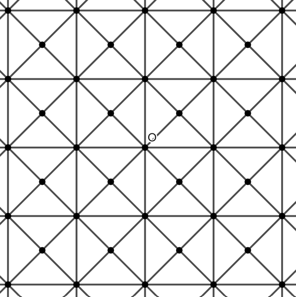
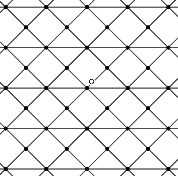
Figure 1. The graph on the left belongs to $\mathcal{G}(4)$, hence it is invariant under rotation of $\pi/2$. The graph on the right is only invariant under rotation of $\pi$.

Now, we introduce the class of plane graphs $\mathcal{G}(a)$ with $a\in\{3,4,6\}$ that is the collection of connected infinite graphs (with finite maximal degree) satisfying conditions (C1)-(C3) with $\theta=\theta(a)=2\pi/a$. It is immediate to notice that $\mathcal{G}(6)\subset\mathcal{G}(3)$. Let, furthermore, $\mathcal{G}:=\mathcal{G}(3)\cup\mathcal{G}(4)$. In Section 4, we will provide various examples of such graphs.

2.3. The $\mathbf{I(G,p)}$-model

We consider the stochastic process $(\sigma_{t})_{t\geq 0}$, which describes $\pm 1$ spin flips dynamics on an infinite graph $G=(V,E)$ with $\Delta(G)<\infty$. The state space is $\Sigma=\{+1,-1\}^{V}$ and the initial state is distributed according to a Bernoulli product measure with density $p\in[0,1]$ of spins $+1$ and $1-p$ of spins $-1$. The process corresponds to the zero-temperature limit of Glauber dynamics for an Ising model with formal Hamiltonian

$$\mathcal{H}(\sigma)=-\sum_{\begin{subarray}{c}u,v\in V:\\ \{u,v\}\in E\end{subarray}}\sigma(u)\sigma(v),$$ (9)

where $\sigma\in\Sigma$. The definition (9) is not well posed for infinite graphs. For this reason, we introduce the changes in energy at vertex $v\in V$ as

$$\Delta\mathcal{H}_{v}(\sigma)=2\sum_{\begin{subarray}{c}u\in V:\\ \{u,v\}\in E\end{subarray}}\sigma(u)\sigma(v).$$

The process $(\sigma_{t})_{t\geq 0}$ is a Markov process on $\Sigma$ with infinitesimal generator having as flip rates

$$c_{t}(v,\sigma)=\begin{cases}0&\text{if $\Delta\mathcal{H}_{v}(\sigma)>0$}\\ \frac{1}{2}&\text{if $\Delta\mathcal{H}_{v}(\sigma)=0$ }\\ 1&\text{if $\Delta\mathcal{H}_{v}(\sigma)<0$}.\end{cases}$$ (10)

It is immediate to notice that the stochastic process is well defined, indeed the supremum in (2) is bounded by $\Delta(G)$ (see [24]). We note that the process is a Glauber attractive dynamics. Furthermore, since $\Delta(G)<\infty$, the flip rates in (10) satisfy the condition in (5) with $A_{v}=N_{V}(v)$. Therefore, this process can be constructed by the Harris’ graphical representation (see [20, 22, 23, 24]). In the following, we will refer to this model as $I(G,p)$-model where $G$ is the underlying graph and $p$ is the density of the Bernoulli product measure for the initial configuration. Now, in Theorem 2, we show that the shrink property is a necessary condition to obtain that the $I(G,p)$-model is of type $\mathcal{I}$.

Theorem 2.

Let $G=(V,E)$ be a graph with $\Delta(G)<\infty$. If $G$ does not have the shrink property then for any $p\in[0,1]$ the $I(G,p)$-model is not of type $\mathcal{I}$.

Proof.

First let us consider the case $p\in(0,1]$. Since $G$ does not have the shrink property then there exists a finite subset $S\subset V$ such that $deg_{V\setminus S}(u)<deg_{S}(u)$ for any $u\in S$. Moreover, one has

$${\mathbb{P}}\biggl{(}\bigcap_{u\in S}\{\sigma_{0}(u)=+1\}\biggr{)}=p^{|S|}>0.$$ (11)

Since $deg_{V\setminus S}(u)<deg_{S}(u)$ for every $u\in S$, no site in $S$ can change the value of its spin if $\sigma_{0}(u)=+1$ for each $u\in S$.

This fact implies that

$${\mathbb{P}}\bigl{(}\text{each vertex in $S$ fixates at the value $+1$ from time zero}\bigr{)}\geq p^{|S|}>0.$$

Thus, for any $p\in(0,1]$ the $I(G,p)$-model is not of type $\mathcal{I}$.

Let us now consider $p=0$. In this case, all sites fixate from time $0$ at the value $-1$ almost surely and the $I(G,0)$-model is of type $\mathcal{F}$. ∎

Remark 2.

Note that Theorem 2 does not imply that the $I(G,p)$-model is of type $\mathcal{F}$ or ${\mathcal{M}}$. In fact if the graph $G$ is not invariant under translation it could happen that the model does not belong to any of the three classes $\mathcal{F},\,{\mathcal{M}}$ and $\mathcal{I}$.

If $G$ does not have the shrink property, it is possible to show examples in which the $I(G,p)$-model is respectively of type $\mathcal{F}$ or ${\mathcal{M}}$. It is known (see [5, 27]) that if $G$ is the hexagonal lattice then the $I(G,p)$-model is of type $\mathcal{F}$. Now, we show in Example 1 that if we consider $G\in\mathcal{G}(4)$ as in Figure 2 then for any $p\in(0,1)$ the $I(G,p)$-model is of type ${\mathcal{M}}$.

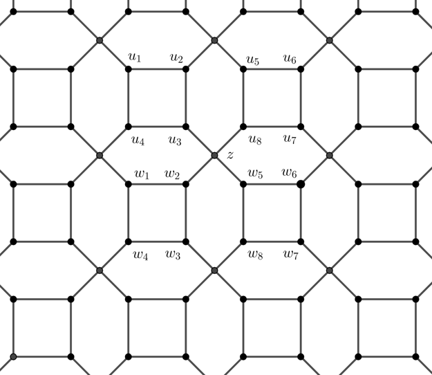
Figure 2. Example of a graph $G\in\mathcal{G}(4)$ that does not have the shrink property and, for $p\in(0,1)$, the $I(G,p)$-model is of type ${\mathcal{M}}$.

Example 1.

Let $G\in\mathcal{G}$ be the graph in Figure 2. For any $p\in(0,1)$ the $I(G,p)$-model is of type ${\mathcal{M}}$. Let $u_{i}\in V$ with $deg(u_{i})=3$ for $i=1,\dots,8$ as in Figure 2. Let $S=\{u_{1},\dots,u_{4}\}$. Since $deg_{V\setminus S}(u_{1})=1<2=deg_{S}(u_{1})$, it is immediate to notice that

$${\mathbb{P}}\bigl{(}\text{$u_{1}$ fixates at the value $+1$}\bigr{)}\geq{\mathbb{P}}\bigl{(}\forall i=1,\dots,4\ \sigma_{0}(u_{i})=+1\bigr{)}=p^{4}>0.$$ (12)

Hence, by ergodicity (see [25, 27]), there exist vertices that fixate at the value $+1$ almost surely. Now, let $z,w_{i}\in V$ be the vertices such that $deg(z)=4$ and $deg(w_{i})=3$ for $i=1,\dots,8$ as in Figure 2. Let $E_{z}$ be the event that the vertices $u_{i}$ and $w_{i}$ fixate respectively at the value $+1$ and $-1$ for each $i=1,\dots,8$. With the same argument used in (12), we deduce that ${\mathbb{P}}(E_{z})\geq p^{8}(1-p)^{8}>0$. Moreover, conditioning on the event $E_{z}$, whenever there is an arrival of the Poisson process ${\mathcal{P}}_{z}$ the spin flip at $z$ occurs with probability $1/2$. Thus, by Lévy’s extension of the Borel-Cantelli Lemmas, $z$ flips infinitely often with positive probability. By ergodicity (see [25, 27]), it follows that there exist vertices that flip infinitely often almost surely. Therefore, the $I(G,p)$-model is of type ${\mathcal{M}}$.

3. Main results

In the following, given $\sigma\in\Sigma$ and $v\in V$, we denote by $C_{v}(\sigma)$ the cluster at site $v$ for $\sigma$, defined as the maximal connected subset of $V$ such that $v\in C_{v}(\sigma)$ and for any $u\in C_{v}(\sigma)$ one has $\sigma(u)=\sigma(v)$.

Now, we present the following theorem, which is an extension of Proposition 3.1 in [4].

Theorem 3.

For $d\in\mathbb{N}$, take a $I(G,p)$-model, where $p\in[0,1]$ and $G$ is a graph embedded in $\mathbb{R}^{d}$ that is translation invariant with respect to $d$ linearly independent vectors. Moreover, suppose that $G$ has the shrink property and $\Delta(G)<\infty$. Then, the size of the cluster at a vertex $v\in V$ diverges almost surely as $t\to\infty$, i.e.

$$\forall v\in V,\quad\lim_{t\to\infty}|C_{v}(\sigma_{t})|=\infty\quad\text{almost surely}.$$

Proof.

We explicitly use the elements $\omega$ of the sample space $\Omega$. We prove the theorem by contradiction. Hence, for a vertex $v\in V$, let us define the event

$$\mathcal{A}:=\{\omega\in\Omega:\liminf_{t\to\infty}|C_{v}(\sigma_{t})|<\infty\}.$$

By contradiction assumption we suppose $\mathbb{P}(\mathcal{A})>0$. By continuity of the measure there exists $M>0$ such that $\mathbb{P}(\mathcal{A}_{M})>0$, where

$$\mathcal{A}_{M}:=\{\omega\in\Omega:\liminf_{t\to\infty}|C_{v}(\sigma_{t})|<M\}.$$

Then, for any $\omega\in\mathcal{A}_{M}$, one can define $(T_{k}(\omega))_{k\in\mathbb{N}}$ such that

$$T_{1}(\omega)=\inf\{t\geq 0:|C_{v}(\sigma_{t})|<M\},$$

and, for $k\in\mathbb{N}$, one recursively defines

$$T_{k+1}(\omega)=\inf\{t\geq T_{k}(\omega)+1:|C_{v}(\sigma_{t})|<M\}.$$

Let $\mathcal{F}_{t}$ be the $\sigma$-algebra generated by the process up to time $t$. It is immediate to note that $T_{k}$ is a stopping time with respect to the filtration $(\mathcal{F}_{t})_{t\geq 0}$ for any $k\in\mathbb{N}$. We consider $\mathcal{F}_{T_{k}}$ for any $k\in\mathbb{N}$. We notice that for $\omega\in\mathcal{A}_{M}$, since $\Delta(G)<\infty$ and $|C_{v}(\sigma_{T_{k}})|<M$, the cluster $C_{v}(\sigma_{T_{k}})$ can be equal only to a finite number of sets of vertices. For each of these sets of vertices, by the shrink property there is an ordered finite sequence of clock rings and outcomes of tie-breaking coin tosses inside a fixed finite ball that would cause the cluster to shrink to a single site $w\in V$ with $d_{G}(w,v)<M$ ($w$ could, in principle, depend on $C_{v}(\sigma_{T_{k}})$). Then, since the vertex $w$ would have all neighbours with opposite spins, it could have an energy-lowering spin flip (with change in energy equal to $-2deg(w)$) and the cluster would vanish with positive probability. We define

$${\mathcal{B}}_{M,k}:=\bigcup_{\begin{subarray}{c}w\in V:\\ d_{G}(w,v)<M\end{subarray}}\bigl{\{}\text{spin at $w$ flips at time $t\in(T_{k},T_{k}+1)$ with $\Delta\mathcal{H}_{w}(\sigma_{t})\leq-1$}\bigr{\}}.$$

From the previous statements in this proof, one has that there exists $\delta>0$ such that

$${\mathbb{P}}\bigl{(}{\mathcal{B}}_{M,k}|\sigma_{T_{k}}\bigr{)}\geq\delta.$$

Now, by the Strong Markov property of the process, for any $k\in\mathbb{N}$ we have the following lower bound

$$\xi_{k}(\omega):=\mathbb{P}\bigl{(}{\mathcal{B}}_{M,k}|\mathcal{F}_{T_{k}}\bigr{)}(\omega)={\mathbb{P}}\bigl{(}{\mathcal{B}}_{M,k}|\sigma_{T_{k}}\bigr{)}\geq\delta,$$

for almost every $\omega\in\mathcal{A}_{M}$. Thus $\sum_{k=1}^{\infty}\xi_{k}(\omega)=\infty$, for almost every $\omega\in\mathcal{A}_{M}$. Now, by using the Lévy’s extension of Borel-Cantelli Lemmas (see e.g. [28]) with the sequence of events $({\mathcal{B}}_{M,k})_{k\in\mathbb{N}}$ and the filtration $(\mathcal{F}_{T_{k}})_{k\in\mathbb{N}}$, we have that

$$\left\{\omega\in\Omega:\sum_{k=1}^{\infty}\xi_{k}(\omega)=\infty\right\}\subset\left\{\omega\in\Omega:\sum_{k=1}^{\infty}\mathbf{1}_{{\mathcal{B}}_{M,k}}(\omega)=\infty\right\}\cup C$$

where $C$ has measure zero. Then

$${\mathbb{P}}\bigl{(}\limsup_{k\to\infty}{\mathcal{B}}_{M,k}\bigr{)}\geq{\mathbb{P}}\bigl{(}\mathcal{A}_{M}\bigr{)}>0.$$

Thus, there exists a vertex $\tilde{w}$ with $d_{G}(\tilde{w},v)<M$ such that energy-lowering spin flips occur at $\tilde{w}$ infinitely many times with positive probability. By translation invariance with respect to $d$ linearly independent vectors, $v_{1},\ldots,v_{d}$, we obtain that the graph $G$ is quasi-transitive. The classes of the graph are all represented inside the parallelogram spanned by the $d$ vectors $v_{1},\ldots,v_{d}$. Now, the translation-ergodicity implies that there exists a positive density of vertices for which energy-lowering spin flips occur infinitely often almost surely. This fact contradicts Theorem 3 and related remark in [27] (see also Lemma 5 in [7]). This concludes the proof. ∎

Remark 3.

Theorem 3 is a generalization of Proposition 3.2 in [4] for graphs $G$ having the shrink property. In [4], the result was given only for the cubic lattice $Z^{d}$ that in particular has the shrink property.

In the following, we consider the $I(G,p)$-model having $G\in\mathcal{G}(a)$ for $a\in\{3,4\}$ and it is invariant under translation with respect to $\bar{x}$. Without loss of generality we take $\bar{x}=(1,0)$. Let us consider a vertex $\tilde{v}$ having minimal Euclidean distance from the origin $O$. Clearly, $\tilde{v}=O$ when $O$ belongs to $V$. In the case $\tilde{v}\neq O$ we consider the two distinct vertices $\tilde{v},R_{\theta}(\tilde{v})$; since $G$ is a connected graph, we can select a connected finite set $S\subset V$ such that $\tilde{v},R_{\theta}(\tilde{v})\in S$. Finally we define the set of vertices

$$U=\bigg{\{}\begin{array}[]{ll}\{O\}&\text{if }O\in V\\ \bigcup_{k=0}^{a-1}R_{k\theta(a)}(S)&\text{otherwise},\\ \end{array}$$ (13)

where $\theta(a)=2\pi/a$. By construction $U$ is connected and $R_{\theta(a)}(U)=U$.

For $a\in\{3,4\}$ we construct a region of size $L\in\mathbb{R}_{+}$ centered in $O$ as follows. Let us consider the point $P_{1}(L,a)=(L\tan(\theta(a)/2),L)\in\mathbb{R}^{2}$ and let

$$P_{i+1}(L,a)=R_{i\theta(a)}(P_{1}),$$

for $i=1,\ldots,a-1$. We define the region of size $L\in\mathbb{R}_{+}$ centered in $O$ as follows

$$T_{L}(a):=Conv(\{P_{1}(L,a),\ldots,P_{a}(L,a)\}).$$

For $a=3,4$ one respectively obtains that $T_{L}(a)$ is an equilateral triangle or a square.

Now, let us consider the class $V_{1}\subseteq V$ (see Theorem 1 and Definition 4). If the graph $G=(V,E)$ is transitive then $V_{1}=V$. We write every vertex $v\in V$ as $v=(v_{x},v_{y})\in\mathbb{R}^{2}$ and let $v_{0,y}:=\max_{v\in V_{1}\cap T_{L}(a)}v_{y}$ and $v_{0,x}:=\min\{v_{x}\in\mathbb{R}:(v_{x},v_{y})\in V_{1}\cap T_{L}(a)\text{ and }v_{y}=v_{0,y}\}$. We define $v_{0}=(v_{0,x},v_{0,y})\in V_{1}\cap T_{L}(a)$. By translation invariance of $G$ with respect to $\bar{x}=(1,0)$, one has $v_{0}+\bar{x}\in V_{1}$. Now we can select a connected set of vertices $U_{0}$ such that $V_{1}\cap B(v_{0},2)\subset U_{0}$. Finally we choose $r_{1}\geq 2$ such that $U_{0}\subset B(v_{0},r_{1})$. We are ready to present the following lemma.

Lemma 4.

For any $G\in\mathcal{G}(a)$ with $a\in\{3,4\}$ and for any $L\in\mathbb{R}_{+}$ there exists a connected set of vertices $W_{L}\subset(T_{L+2r_{1}}(a)\setminus T_{L-2r_{1}}(a))$ such that $R_{\theta(a)}(W_{L})=W_{L}$.

Proof.

For $k\in\mathbb{N}$, let

$$v_{k}:=v_{0}+k\bar{x}.$$

We define $k_{max}=\max\{k\in\mathbb{N}:v_{k}\in T_{L}(a)\}$. The set of vertices

$${\mathcal{S}}=\bigcup_{k=0}^{k_{max}}(U_{0}+k\bar{x})$$

is connected because for any $k=0,\ldots,k_{max}-1$ it turns out that $G[U_{0}+k\bar{x}]$ is connected and $v_{k},v_{k+1}\in U_{0}+k\bar{x}$.

We define the set of vertices $W_{L}=\bigcup_{i=0}^{a-1}R_{i\theta(a)}({\mathcal{S}})$. Now, we show that $W_{L}$ is connected. Since

$$||v_{0}-P_{2}(L,a)||\leq 1,\quad||P_{1}(L,a)-v_{k_{max}}||\leq 1$$

and by using the triangular inequality, one obtains

$$||v_{0}-R_{\theta(a)}(v_{k_{max}})||\leq||v_{0}-P_{2}(L,a)||+||P_{2}(L,a)-R_{\theta(a)}(v_{k_{max}})||=\\ =||v_{0}-P_{2}(L,a)||+||P_{1}(L,a)-v_{k_{max}}||\leq 2.$$

The previous inequality and $V_{1}\cap B(v_{0},2)\subset U_{0}$ imply that $W_{L}$ is connected. Clearly $W_{L}\subset(T_{L+2r_{1}}(a)\setminus T_{L-2r_{1}}(a))$ and $R_{\theta(a)}(W_{L})=W_{L}$. ∎

Let $W_{L}$ as in Lemma 4. One can select a cycle $U_{L}\subset W_{L}$; we call $f_{L,\infty}$ its outer face and $f_{L,0}$ its inner face.

Remark 4.

We notice that, by translational invariance with respect to the vectors $\bar{x}=(1,0)$ and $\bar{y}=(\cos\theta(a),\sin\theta(a))$, one has

$$|W_{L}|\asymp L\quad\text{and}\quad|V\cap f_{L,0}|\asymp L^{2},$$

where we write $a_{n}\asymp b_{n}$ to mean that there exist two positive constants $c_{1}$ and $c_{2}$ such that $c_{1}\leq\frac{a_{n}}{b_{n}}\leq c_{2}$ for all $n\in\mathbb{N}$. This implies that $G\in\mathcal{G}(a)$ is amenable for any $a\in\{3,4,6\}$. Under the assumptions of amenability of the graph, the translation invariance of the measure $\mu$ and finite-energy of the measure $\mu$, it is known that the infinite cluster is at most one almost surely (see [2, 3, 19]). For the zero-temperature stochastic Ising model, it is not known whether the measure induced at time $t$ has finite-energy property. Therefore, we are not able to prove the uniqueness of the infinite cluster at time $t$. Instead, if the temperature is positive and decreases to zero, one has the property of finite-energy (see [7]). In this last case one obtains the uniqueness of the infinite cluster.

Now, given an integer $q\in\mathbb{N}$ and $\delta<\frac{1}{2q}$, we consider $T_{1+\delta}(a)\setminus T_{1-\delta}(a)$ and we show that there exists a collection of balls $(B(c_{i},4/q):i=1,\ldots,aq)$ such that:

• $T_{1+\delta}(a)\setminus T_{1-\delta}(a)\subset\bigcup_{i=1}^{aq}B(c_{i},4/q)$;

• for any $i=1,\ldots,aq$, the center $c_{i}$ belongs to $\partial T_{1}(a)$;

• for any $i=1,\ldots,q$ and $m=0,\ldots,a-1$ one has $c_{i+mq}=R_{m\theta(a)}(c_{i})$. In particular, $R_{\theta(a)}(\bigcup_{i=1}^{aq}B(c_{i},4/q))=\bigcup_{i=1}^{aq}B(c_{i},4/q)$.

It is clear that such a construction exists, for example by taking the centers of the ball equally spaced. The chosen balls in this construction will be maintained also in the sequel.

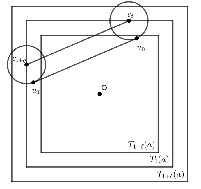
Figure 3. The distance between the segment having $u_{0}\in B(c_{i},4/q)$ and $u_{1}\in B(c_{i+q},4/q)$ as its endpoints and $O$ can decrease at most of $4/q$ (the length of the radius) with respect to the distance between the segment having endpoins $c_{i}$ and $c_{i+q}$ and $O$.

Lemma 5 (Geometric Lemma).

Let $a\in\{3,4\}$, $q\geq 10$ and $\delta<\frac{1}{2q}$ and consider the cover of $T_{1+\delta}(a)\setminus T_{1-\delta}(a)$ introduced in items a, b, and c. Then, for any $(u_{k})_{k=0,\ldots,a-1}$ such that $u_{k}\in B(c_{i+kq},4/q)$ for $k=0,\ldots,a-1$, one has $Conv(\{u_{0},\ldots,u_{a-1}\})\supset B(O,\frac{1}{2}-\frac{4}{q})$.

Proof.

For a fixed $i=1,\ldots,q$, let us consider $(c_{i+kq})_{k=0,\ldots,a-1}$. For $a=3,4$, we note that $Conv(\{c_{i+kq}:k=0,\ldots,a-1\})$ is an equilateral triangle or a square. Therefore, since $c_{i+kq}\in\partial T_{1}(a)$ one has $Conv(\{c_{i+kq}:k=0,\ldots,a-1\})\supset B(O,\frac{1}{2})$. Let us now consider the segment having $u_{0}\in B(c_{i},4/q)$ and $u_{1}\in B(c_{i+q},4/q)$ as its endpoints. The distance between this segment and the origin $O$ can decrease at most of $4/q$ with respect to the distance between $O$ and the segment having endpoins $c_{i},c_{i+q}$ (see Figure 3). Then one obtains that $Conv(\{u_{0},\ldots,u_{a-1}\})\supset B(O,\frac{1}{2}-\frac{4}{q})$. ∎

As already announced, we do not deal with $\theta=\pi$. Indeed if we consider $a=2$ which corresponds to $\theta(a)=\pi$, this statement is false because $Conv(\{u_{0},u_{1}\})$ would be a segment and there is no ball contained in it. From now on we take $q\geq 24$ and hence $\frac{1}{2}-\frac{4}{q}\geq\frac{1}{3}$.

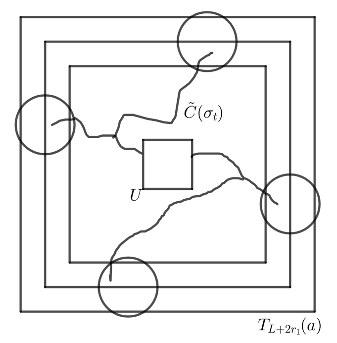
Figure 4. Example of a realization of an $L$-cross.

Now, we present the following definition.

Definition 7 ($L$-Cross).

Given $G\in\mathcal{G}(a)$ with $a\in\{3,4\}$, we say that an $L$-cross of $+1$ occurs at time $t$ if there exists a cluster $\tilde{C}(\sigma_{t})$ of $G[V\cap T_{L+2r_{1}}(a)]$ such that

• $\sigma_{t}(v)=+1$ for each $v\in\tilde{C}(\sigma_{t})$;

• $\tilde{C}(\sigma_{t})\supset U$, where $U$ is defined in (13);

• there exists $i\in\{1,\dots,q\}$ such that $\tilde{C}(\sigma_{t})\cap B(Lc_{i+kq},\,4L/q)\neq\emptyset$ for each $k=0,\dots,a-1$.

We denote by $E^{t}_{L}$ with $t\in\mathbb{R}_{0}^{+}$ the event that an $L$-cross of $+1$ occurs at time $t$. Moreover, we define

$$A_{L}:=\limsup_{t\to\infty}E^{t}_{L}.$$ (14)

We define the set of vertices $S_{L}(t):=\tilde{C}(\sigma_{t})\cap W_{L}$, where the properties of $W_{L}$ are given in Lemma 4. The previous Lemma 5 shows that for each time $t\in\mathbb{R}_{0}^{+}$ in which an $L$-cross of $+1$ occurs (see Figure 4), one has

$$Conv(S_{L}(t))\supset B\left(O,r_{L}\right)\quad\text{where $r_{L}=\frac{1}{3}L$}.$$ (15)

In other words, Lemma 5 says that $|Conv_{G}(S_{L}(t))|\asymp L^{2}$.

Lemma 6.

Consider the $I(G,p)$-model, where $p\in[\frac{1}{2},1)$ and $G\in\mathcal{G}$. If $G$ has the shrink property, then

$${\mathbb{P}}(A_{L})\geq p_{cross}:=\frac{1}{(aq)^{a}}\left(\frac{1}{2}\right)^{a|U|},$$

where the event $A_{L}$ is defined in (14).

We now explain the strategy for proving Lemma 6. Let $U\subset V$ as defined in (13). If the initial density $p\geq 1/2$, then $U$ is contained in a cluster of $+1$ with probability at least $(1/2)^{|U|}$, at any time $t$. By Theorem 3, the size of this cluster diverges almost surely as $t\to\infty$. Now, by FKG inequality and by rotation invariance, one obtains that $\liminf_{t\to\infty}{\mathbb{P}}(E^{t}_{L})>0$, i.e. the cluster satisfies the properties in Definition 7 with positive probability. Note that this lower bound does not depend on $L$. By Reverse Fatou Lemma, we obtain the same lower bound on ${\mathbb{P}}(A_{L})$. We are now ready to prove the lemma.

Proof.

Let ${\mathcal{U}}_{t}$ be the event that all vertices in $U$ have spin equal to $+1$ at time $t$. By Lemma 1, FKG inequality and Harris’ inequality (see [24, 21]), it follows that

$${\mathbb{P}}({\mathcal{U}}_{t})\geq\biggl{(}\frac{1}{2}\biggr{)}^{|U|}.$$ (16)

If ${\mathcal{U}}_{t}$ occurs, then, since $U$ is connected, at time $t$ all vertices in $U$ belong to a same cluster, we call it $C_{U}(\sigma_{t})$. Moreover, let $\tilde{C}(\sigma_{t})$ be the cluster of $G[V\cap T_{L+2r_{1}}(a)]$ that contains $U$. We denote by ${\mathcal{C}}_{W_{L}}(t)$ the event that the cluster $\tilde{C}(\sigma_{t})$ intersects $W_{L}$, i.e. ${\mathcal{C}}_{W_{L}}(t):=\{\tilde{C}(\sigma_{t})\cap W_{L}\neq\emptyset\}$. By Theorem 3, we have that $\lim_{t\to\infty}|C_{U}(\sigma_{t})|=\infty$ almost surely. Thus, by planarity of $G$ and $V\cap f_{L,0}$ has finite cardinality (see Remark 4), we get

$$\lim_{t\to\infty}{\mathbb{P}}\bigl{(}{\mathcal{C}}_{W_{L}}(t)\bigr{)}=1.$$ (17)

By (16) and (17), it follows that

$$\liminf_{t\to\infty}\mathbb{P}\bigl{(}{\mathcal{C}}_{W_{L}}(t)\cap{\mathcal{U}}_{t}\bigr{)}=\liminf_{t\to\infty}{\mathbb{P}}({\mathcal{U}}_{t})\geq\biggl{(}\frac{1}{2}\biggr{)}^{|U|}.$$ (18)

Now, we write $W_{L}=\cup_{i=1}^{q}\cup_{k=0}^{a-1}P_{L,k}^{i}$ where $P_{L,k}^{i}:=W_{L}\cap B(Lc_{i+kq},\,4L/q)$ for $i=1,\dots,q$ and $k=0,\dots,a-1$. We define the event ${\mathcal{C}}_{L,i,k}(t):=\{\tilde{C}(\sigma_{t})\cap P_{L,k}^{i}\neq\emptyset\}$ for $i=1,\dots,q$ and $k=0,\dots,a-1$. Hence, we have

$${\mathcal{C}}_{W_{L}}(t)\cap{\mathcal{U}}_{t}=\bigcup_{i=1}^{q}\bigcup_{k=0}^{a-1}{\mathcal{C}}_{L,i,k}(t)\cap{\mathcal{U}}_{t}.$$

Thus, by rotation invariance and by the union bound, we have

$$\mathbb{P}\bigl{(}{\mathcal{C}}_{W_{L}}(t)\cap{\mathcal{U}}_{t}\bigr{)}={\mathbb{P}}\biggl{(}\bigcup_{i=1}^{q}\bigcup_{k=0}^{a-1}\bigl{(}{\mathcal{C}}_{L,i,k}(t)\cap{\mathcal{U}}_{t}\bigr{)}\biggr{)}\leq\sum_{i=1}^{q}\sum_{k=0}^{a-1}{\mathbb{P}}\bigl{(}{\mathcal{C}}_{L,i,k}(t)\cap{\mathcal{U}}_{t}\bigr{)}\leq\\ \leq aq{\mathbb{P}}\bigl{(}{\mathcal{C}}_{L,\bar{i},0}(t)\cap{\mathcal{U}}_{t}\bigr{)},$$ (19)

where $\bar{i}\in\{1,\dots,q\}$ is such that ${\mathbb{P}}\bigl{(}{\mathcal{C}}_{L,\bar{i},0}(t)\cap{\mathcal{U}}_{t}\bigr{)}=\max_{i=1,\dots,q}{\mathbb{P}}\bigl{(}{\mathcal{C}}_{L,i,0}(t)\cap{\mathcal{U}}_{t}\bigr{)}$. We note that ${\mathcal{C}}_{L,\bar{i},k}(t)\cap{\mathcal{U}}_{t}$ is an increasing event for $k=0,\dots,a-1$; therefore

$${\mathbb{P}}\biggl{(}\bigcap_{k=0}^{a-1}\bigl{(}{\mathcal{C}}_{L,\bar{i},k}(t)\cap{\mathcal{U}}_{t}\bigr{)}\biggr{)}\geq\biggl{(}{\mathbb{P}}\bigl{(}{\mathcal{C}}_{L,\bar{i},0}(t)\cap{\mathcal{U}}_{t}\bigr{)}\biggr{)}^{a}\geq\biggl{(}\frac{1}{aq}\mathbb{P}\bigl{(}{\mathcal{C}}_{W_{L}}(t)\cap{\mathcal{U}}_{t}\bigr{)}\biggr{)}^{a},$$ (20)

where the first inequality follows by FKG inequality and by rotation invariance, and the last inequality follows by (19). We also notice that, by definition of $P_{L,k}^{i}$, one has

$${\mathcal{C}}_{L,i,k}(t)=\{\tilde{C}(\sigma_{t})\cap P_{L,k}^{i}\neq\emptyset\}\subset\{\tilde{C}(\sigma_{t})\cap B(Lc_{i+kq},\,4L/q)\neq\emptyset\}.$$

Thus, by Definition 7, we have

$$E^{t}_{L}=\bigcup_{i=1}^{q}\bigcap_{k=0}^{a-1}\bigl{\{}\tilde{C}(\sigma_{t})\cap B(Lc_{i+kq},\,4L/q)\neq\emptyset\bigr{\}}\cap{\mathcal{U}}_{t}\supseteq\\ \supseteq\bigcup_{i=1}^{q}\bigcap_{k=0}^{a-1}{\mathcal{C}}_{L,i,k}(t)\cap{\mathcal{U}}_{t}\supseteq\bigcap_{k=0}^{a-1}{\mathcal{C}}_{L,\bar{i},k}(t)\cap{\mathcal{U}}_{t},$$

and hence

$$\mathbb{P}(E^{t}_{L})\geq{\mathbb{P}}\biggl{(}\bigcap_{k=0}^{a-1}{\mathcal{C}}_{L,\bar{i},k}(t)\cap{\mathcal{U}}_{t}\biggr{)}.$$ (21)

Now, by (18), (20) and (21), we obtain the following lower bound

$$\liminf_{t\to\infty}\mathbb{P}(E^{t}_{L})\geq\liminf_{t\to\infty}\biggl{(}\frac{1}{aq}\mathbb{P}\bigl{(}{\mathcal{C}}_{W_{L}}(t)\cap{\mathcal{U}}_{t}\bigr{)}\biggr{)}^{a}\geq\frac{1}{(aq)^{a}}\left(\frac{1}{2}\right)^{a|U|}.$$

Finally, by Reverse Fatou Lemma we get

$$\mathbb{P}(A_{L})\geq\limsup_{t\to\infty}\mathbb{P}(E^{t}_{L})\geq\liminf_{t\to\infty}\mathbb{P}(E^{t}_{L})\geq\frac{1}{(aq)^{a}}\left(\frac{1}{2}\right)^{a|U|}>0$$

that concludes the proof. ∎

Now we give a simple definition that will be useful when related to $E^{t}_{L}$ through Lemma 5. For $t\in\mathbb{R}_{0}^{+}$, let $F^{t}_{L}$ be the event that all sites belonging to $B(O,\frac{L}{3})$ have spin equal to $+1$ at some time $s\in(t,t+1)$.

Lemma 7.

Consider the $I(G,p)$-model, where $p\in[\frac{1}{2},1)$ and $G\in\mathcal{G}$. If $G$ has the planar shrink property, then there exists $\epsilon_{L}>0$ such that

$$\mathbb{P}(F^{t}_{L}|\sigma_{t}=\sigma)\geq\epsilon_{L}$$

for any $\sigma\in\Sigma$ such that $\{\sigma_{t}=\sigma\}\subset E^{t}_{L}$.

Proof.

Let $\sigma\in\Sigma$ and $(\sigma_{s})_{s\geq 0}$ be the $I(G,p)$-model such that $\{\sigma_{t}=\sigma\}\subset E^{t}_{L}$. We define another zero-temperature stochastic Ising model $(\sigma_{s}^{\prime})_{s\geq t}$ with infinitesimal generator having the flip rates as in (10) and such that

$$\sigma_{t}^{\prime}(v)=\begin{cases}+1&\text{for each $v\in\tilde{C}(\sigma_{t})$}\\ -1&\text{otherwise},\end{cases}$$

where $\tilde{C}(\sigma_{t})$ is the cluster of $G[V\cap T_{L+2r_{1}}(a)]$ in the configuration $\sigma$, as in Definition 7. By definition of $\sigma_{t}^{\prime}$ and $E^{t}_{L}$, $\tilde{C}(\sigma_{t})\supset U$ is the unique cluster of $+1$ sites in the configuration $\sigma_{t}^{\prime}$. In configuration $\sigma_{t}^{\prime}$, we have that $\bigl{(}V\cap T_{L+2r_{1}}(a)\bigr{)}\setminus\tilde{C}(\sigma_{t})=D_{1}(\sigma_{t}^{\prime})\sqcup\dots\sqcup D_{k}(\sigma_{t}^{\prime})$, where $D_{i}(\sigma_{t}^{\prime})$ for $i=1,\dots,k$ are clusters of $-1$ sites (we stress that $k<\infty$ because $V\cap T_{L+2r_{1}}(a)$ has finite cardinality).

We notice that, by planarity of $G$, for each $i=1,\dots,k$ we have that $\partial_{ext}D_{i}(\sigma_{t}^{\prime})\subset\tilde{C}(\sigma_{t})$. By planar shrink property, for each $i=1,\dots,k$ there exists an ordered finite sequence of updates (i.e. of clock rings and outcomes of tie-breaking coin tosses inside $V\cap T_{L+2r_{1}}(a)$) that would cause all sites of $D_{i}(\sigma_{t}^{\prime})\cap Conv_{G}(S_{L}(t))$ (see definition above formula (15)) to have spin equal to $+1$ in some time $s\in(t,t+1)$ with positive probability. Therefore, we get an ordered finite sequence of updates inside $V\cap T_{L+2r_{1}}(a)$ that would cause all sites of $Conv_{G}(S_{L}(t))$ to have spin equal to $+1$ in $\sigma_{s}^{\prime}$ (with $s\in(t,t+1)$), but since $\sigma_{t}^{\prime}\leq\sigma_{t}$ this sequence of updates works, by the coupling in Lemma 1, in the same way for the original process $(\sigma_{s}:s\in(t,t+1))$. Moreover, by Lemma 5, one has $V\cap B(O,\frac{L}{3})\subset Conv_{G}(S_{L}(t))$.

Thus, there exists $\epsilon_{L}>0$ such that

$$\mathbb{P}(F^{t}_{L}|\sigma_{t}=\sigma)\geq\epsilon_{L}$$

for any $\sigma\in\Sigma$ having $\{\sigma_{t}=\sigma\}\subset E^{t}_{L}$. ∎

We recall that $A_{L}:=\limsup_{t\to\infty}E^{t}_{L}$. Now, we define $B_{L}:=\limsup_{t\to\infty}F^{t}_{L}$. We are ready to present the following lemma.

Lemma 8.

Consider the $I(G,p)$-model, where $p\in[\frac{1}{2},1)$ and $G\in\mathcal{G}$. If $G$ has the planar shrink property, then ${\mathbb{P}}(B_{L})\geq p_{cross}>0$.

Proof.

In the proof we will explicitly use the elements $\omega$ of the sample space $\Omega$. First, let $\omega\in A_{L}$, i.e. an $L$-cross of $+1$ occurs infinitely often. Then one can define $(T_{k}(\omega))_{k\in\mathbb{N}}$ such that

$$T_{1}(\omega)=\inf\{t\geq 0:E^{t}_{L}\text{ occurs}\},$$

and, for $k\in\mathbb{N}$, we recursively define

$$T_{k+1}(\omega)=\inf\{t\geq T_{k}+1:E^{t}_{L}\text{ occurs}\}.$$

Let $\mathcal{F}_{t}$ be the $\sigma$-algebra generated by the process up to time $t$. It is immediate to note that $T_{k}$ is a stopping time with respect to the filtration $(\mathcal{F}_{t})_{t\geq 0}$ for any $k\in\mathbb{N}$. We consider $\mathcal{F}_{T_{k}}$ for any $k\in\mathbb{N}$. By the Strong Markov property of the process and by Lemma 7, for any $k\in\mathbb{N}$ we have the following lower bound

$$\xi_{k}(\omega):=\mathbb{P}\bigl{(}F^{T_{k}}_{L}|\mathcal{F}_{T_{k}}\bigr{)}(\omega)={\mathbb{P}}\bigl{(}F^{T_{k}}_{L}|\sigma_{T_{k}}\bigr{)}\geq\epsilon_{L}>0,$$

for almost every $\omega\in A_{L}$. Thus $\sum_{k=1}^{\infty}\xi_{k}(\omega)=\infty$, for almost every $\omega\in A_{L}$. Now, by using the Lévy’s extension of Borel-Cantelli Lemmas (see e.g. [28]) with the sequence of events $(F^{T_{k}}_{L})_{k\in\mathbb{N}}$ and the filtration $(\mathcal{F}_{T_{k}})_{k\in\mathbb{N}}$, we have that

$$\left\{\omega\in\Omega:\sum_{k=1}^{\infty}\xi_{k}(\omega)=\infty\right\}\subset\left\{\omega\in\Omega:\sum_{k=1}^{\infty}\mathbf{1}_{F^{T_{k}}_{L}}(\omega)=\infty\right\}\cup C,$$

where $C$ has measure zero. Then, by Lemma 6, we get

$${\mathbb{P}}\bigl{(}B_{L}\bigr{)}\geq{\mathbb{P}}\bigl{(}A_{L}\bigr{)}\geq\frac{1}{(aq)^{a}}\left(\frac{1}{2}\right)^{a|U|}=p_{cross}>0.$$

This concludes the proof. ∎

Now, for any time $t_{2}>t_{1}+1$ we define

$$D(L;t_{1},t_{2}):=\bigcup_{s\in[t_{1},t_{2}-1]}F^{s}_{L}\quad\text{and}\quad D(L;t_{1},\infty):=\bigcup_{s\geq t_{1}}F^{s}_{L}.$$

Lemma 9.

For any $L\in\mathbb{R}_{+}$ and $t_{1}\geq 0$, one has

$${\mathbb{P}}\bigl{(}D(L;t_{1},\infty)\bigr{)}\geq p_{cross}.$$

Moreover, for any $\epsilon>0$ there exists a time $s>t_{1}+1$ such that

$${\mathbb{P}}\bigl{(}D(L;t_{1},s)\bigr{)}\geq(1-\epsilon)p_{cross}.$$

Proof.

We observe that $D(L;t_{1},\infty)\supset B_{L}$. In particular, by Lemma 8,

$${\mathbb{P}}\bigl{(}D(L;t_{1},\infty)\bigr{)}\geq p_{cross}.$$

Now, we note that for $t_{2}\leq t_{2}^{\prime}$ one has $D(L;t_{1},t_{2})\subset D(L;t_{1},t_{2}^{\prime})$. Thus, by continuity of measure

$$\lim_{t_{2}\to\infty}{\mathbb{P}}\bigl{(}D(L;t_{1},t_{2})\bigr{)}={\mathbb{P}}\biggl{(}\bigcup_{s\geq t}D(L;t_{1},s)\biggr{)}={\mathbb{P}}\bigl{(}D(L;t_{1},\infty)\bigr{)}\geq p_{cross}.$$

Hence for all $\epsilon>0$ there exists a time $s>t_{1}+1$ such that

$${\mathbb{P}}\bigl{(}D(L;t_{1},s)\bigr{)}\geq(1-\epsilon)p_{cross}.$$

∎

Let $\mathcal{F}$ be the $\sigma$-algebra generated by the process $(\sigma_{t})_{t\geq 0}$. All the events introduced belong to $\mathcal{F}$. Given a non-zero vector $\bar{v}$ such that $G$ is translation invariant with respect to $\bar{v}$, we define the configuration translated with respect to $\bar{v}$ as

$$(\sigma+\bar{v})(v):=\sigma(v+\bar{v})\quad\text{for any $v\in V$}.$$

Let $X$ be a $\mathcal{F}$-measurable random variable. Then $X=f((\sigma_{t})_{t\geq 0})$ where $f$ is a measurable function. We define

$$X+\bar{v}:=f((\sigma_{t}-\bar{v})_{t\geq 0}).$$ (22)

If $X$ is an indicator function then $f$ takes only the values $0$ or $1$. Let $A\in\mathcal{F}$, one can define

$$\mathbf{1}_{A}+\bar{v}=f((\sigma_{t}-\bar{v})_{t\geq 0})=:\mathbf{1}_{A+\bar{v}},$$

that defines $A+\bar{v}$ for any $A\in\mathcal{F}$.

In the following result we will apply the ergodic theorem. We note that these processes are ergodic with respect to the translation if the initial conditions are given for instance by a Bernoulli product measure, see e.g. [20, 24, 25] and references therein. Now, we introduce some notation, which we will use in the proof of Theorem 4. For $v\in V$ and $t\in\mathbb{R}_{+}$, let

$$A^{+}_{v}(t):=\{\sigma_{s}(v)=+1,\ \ \forall s\in[0,t]\},\quad A^{-}_{v}(t):=\{\sigma_{s}(v)=-1,\ \ \forall s\in[0,t]\}.$$

We denote by $A^{+}_{v}(\infty)$ (resp. $A^{-}_{v}(\infty)$) the event that the vertex $v$ fixates at the value $+1$ (resp. $-1$) from time zero. Clearly, $A_{v}^{\pm}(t)\subset A_{v}^{\pm}(t^{\prime})$, for any $t^{\prime}\leq t$. We recall that $\{V_{1},\dots,V_{N}\}$ is the partition of the vertex set $V$ that comes from the quasi-transitivity of $G\in\mathcal{G}$, see Theorem 1. We note that, since $G$ is quasi-transitive, ${\mathbb{P}}(A^{\pm}_{v}(t))$ depends only on the class to which the vertex $v$ belongs and does not depend explicitly on the vertex itself. Thus, for $p=1/2$, for each $i=1,\dots,N$, $v\in V_{i}$, and $t\in\mathbb{R}_{+}\cup\{\infty\}$, we set

$$\rho_{i}(t):={\mathbb{P}}(A^{+}_{v}(t))={\mathbb{P}}(A^{-}_{v}(t)).$$

The last equality follows by symmetry under the global spin flip for $p=1/2$. Now, we are ready to prove our main result.

Theorem 4.

If $G=(V,E)\in\mathcal{G}$ has the planar shrink property, then the $I(G,1/2)$-model is of type $\mathcal{I}$, i.e., all sites flip infinitely often almost surely.

Proof.

We will prove the theorem by contradiction. Suppose that there exists $j\in\{1,\dots,N\}$ such that $\rho_{j}(\infty)>0$ that by Lemma 2 is equivalent to have a site that fixates with positive probability. We choose the following constants: $\epsilon=\frac{1}{3}p_{cross}\rho_{j}(\infty)$, $\epsilon_{1}=\frac{\rho_{j}(\infty)}{5}$, $\epsilon_{2}=\frac{1}{4}p_{cross}$ and $\tilde{\epsilon}=\frac{1}{8}$.

We notice that, by continuity of the measure, the limit of $\rho_{i}(t)$ as $t\to\infty$ exists and is equal to

$$\lim_{t\to\infty}\rho_{i}(t)=\lim_{t\to\infty}{\mathbb{P}}(A^{+}_{v}(t))={\mathbb{P}}\biggl{(}\bigcap_{m=1}^{\infty}A^{+}_{v}(m)\biggr{)}={\mathbb{P}}(A^{+}_{v}(\infty))=\rho_{i}(\infty),$$

for each $v\in V_{i}$. This implies that there exists a time $t_{\epsilon}>0$ such that

$$0\leq\rho_{j}(t_{\epsilon})-\rho_{j}(\infty)<\epsilon.$$ (23)

Since $G\in\mathcal{G}$, there exist two linearly independent vectors $\bar{x}_{1}$ and $\bar{x}_{2}$ such that $G$ is translation invariant with respect to them. We want to construct on the graph $G$ disjoint regions of a suitable size $L_{0}$ centered in $n_{1}\bar{x}_{1}+n_{2}\bar{x}_{2}$ with $n_{1},n_{2}\in\mathbb{Z}$. By ergodicity (see [20, 25, 27]), one has

$$\lim_{r\to\infty}\frac{1}{n(r,j)}\sum_{v\in B(O,r)\cap V_{j}}\mathbf{1}_{A^{-}_{v}(t_{\epsilon})}=\rho_{j}(t_{\epsilon})>0\quad\text{almost surely,}$$ (24)

where $n(r,j):=|B(O,r)\cap V_{j}|$. Thus, (24) implies that there exists $\tilde{r}\in\mathbb{R}_{+}$ such that

$${\mathbb{P}}\biggl{(}\frac{1}{n(\tilde{r},j)}\sum_{v\in B(O,\tilde{r})\cap V_{j}}\mathbf{1}_{A^{-}_{v}(t_{\epsilon})}\notin[\rho_{j}(t_{\epsilon})-\epsilon_{1},\rho_{j}(t_{\epsilon})+\epsilon_{1}]\biggr{)}\leq\epsilon_{2}.$$

Then, in particular

$${\mathbb{P}}\biggl{(}\sum_{v\in B(O,\tilde{r})\cap V_{j}}\mathbf{1}_{A^{-}_{v}(t_{\epsilon})}<n(\tilde{r},j)\bigl{(}\rho_{j}(t_{\epsilon})-\epsilon_{1}\bigr{)}\biggr{)}\leq\epsilon_{2}.$$ (25)

Now, we construct disjoint regions of size $L_{0}$ on the graph $G$ in the following way. Let $L_{0}=3\tilde{r}$, where $L_{0}$ and $\tilde{r}$ play the same role of $L$ and $r_{L}$ in (15). We define the event

$$G(L;t,\eta):=\biggl{\{}\sum_{v\in B(O,L/3)\cap V_{j}}\mathbf{1}_{A^{-}_{v}(t)}\geq n(L/3,j)\bigl{(}\rho_{j}(t)-\eta\bigr{)}\biggr{\}},$$

where $L,t,\eta>0$. By (25), one has

$${\mathbb{P}}\bigl{(}G(L_{0};t_{\epsilon},\epsilon_{1})\bigr{)}\geq 1-\epsilon_{2}.$$ (26)

Now, let

$$Y_{L_{0}}(t):=\sum_{v\in B(O,L_{0}/3)\cap V_{j}}\mathbf{1}_{A^{-}_{v}(t)}.$$

Let $n_{0}\in\mathbb{N}$ such that $T_{L_{0}+2r_{1}}(a)\cap(T_{L_{0}+2r_{1}}(a)+n_{0}\bar{x}_{i})=\emptyset$ for $i=1,2$. We define $Y_{L_{0},m_{1},m_{2}}(t):=Y_{L_{0}}(t)+m_{1}n_{0}\bar{x}_{1}+m_{2}n_{0}\bar{x}_{2}$ with $m_{1},m_{2}\in\mathbb{Z}$ (see (22)). By ergodicity, it follows that for any $t\in\mathbb{R}_{+}$

$$\lim_{M\to\infty}\frac{1}{(2M+1)^{2}}\sum_{\begin{subarray}{c}m_{1},m_{2}\in\mathbb{Z}:\\ |m_{1}|,|m_{2}|\leq M\end{subarray}}\frac{1}{n(L_{0}/3,j)}Y_{L_{0},m_{1},m_{2}}(t)=\rho_{j}(t),\quad\text{a.s.}$$ (27)

We define the translated events

$$D(L;m_{1},m_{2};t_{1},t_{2}):=D(L;t_{1},t_{2})+m_{1}n_{0}\bar{x}_{1}+m_{2}n_{0}\bar{x}_{2}$$

and

$$G(L;m_{1},m_{2};t,\eta):=G(L;t,\eta)+m_{1}n_{0}\bar{x}_{1}+m_{2}n_{0}\bar{x}_{2}.$$

Now, by Lemma 9 and by translation invariance, there exists a time ${t}_{\tilde{\epsilon}}>t_{\epsilon}+1$ such that

$${\mathbb{P}}\bigl{(}D(L_{0};m_{1},m_{2};t_{\epsilon},t_{\tilde{\epsilon}})\bigr{)}\geq(1-\tilde{\epsilon})p_{cross}.$$ (28)

By ergodicity, (26) and (28), it follows that

$$\lim_{M\to\infty}\frac{1}{(2M+1)^{2}}\sum_{\begin{subarray}{c}m_{1},m_{2}\in\mathbb{Z}:\\ |m_{1}|,|m_{2}|\leq M\end{subarray}}\mathbf{1}_{G(L_{0};m_{1},m_{2};t_{\epsilon},\epsilon_{1})\cap D(L_{0};m_{1},m_{2};t_{\epsilon},t_{\tilde{\epsilon}})}=\\ ={\mathbb{P}}\bigl{(}G(L_{0};m_{1},m_{2};t_{\epsilon},\epsilon_{1})\cap D(L_{0};m_{1},m_{2};t_{\epsilon},t_{\tilde{\epsilon}})\bigr{)}\geq\\ \geq{\mathbb{P}}\bigl{(}D(L_{0};m_{1},m_{2};t_{\epsilon},t_{\tilde{\epsilon}})\bigr{)}-{\mathbb{P}}\bigl{(}G(L_{0};m_{1},m_{2};t_{\epsilon},\epsilon_{1})^{c}\bigr{)}\geq(1-\tilde{\epsilon})p_{cross}-\epsilon_{2}\quad\text{a.s.}$$ (29)

Over the event $G(L_{0};m_{1},m_{2};t_{\epsilon},\epsilon_{1})$ one has

$$Y_{L_{0},m_{1},m_{2}}(t_{\epsilon})\geq n(L_{0}/3,j)\bigl{(}\rho_{j}(t_{\epsilon})-\epsilon_{1}\bigr{)}.$$ (30)

By (27), we get

$$\rho_{j}(t_{\epsilon})-\rho_{j}(t_{\tilde{\epsilon}})=\lim_{M\to\infty}\frac{1}{(2M+1)^{2}}\sum_{\begin{subarray}{c}m_{1},m_{2}\in\mathbb{Z}:\\ |m_{1}|,|m_{2}|\leq M\end{subarray}}\frac{1}{n(L_{0}/3,j)}\biggl{[}Y_{L_{0},m_{1},m_{2}}(t_{\epsilon})-Y_{L_{0},m_{1},m_{2}}(t_{\tilde{\epsilon}})\biggr{]}\geq\\ \geq\lim_{M\to\infty}\frac{1}{(2M+1)^{2}}\sum_{\begin{subarray}{c}m_{1},m_{2}\in\mathbb{Z}:\\ |m_{1}|,|m_{2}|\leq M\end{subarray}}\frac{1}{n(L_{0}/3,j)}Y_{L_{0},m_{1},m_{2}}(t_{\epsilon})\mathbf{1}_{G(L_{0};m_{1},m_{2};t_{\epsilon},\epsilon_{1})\cap D(L_{0};m_{1},m_{2};t_{\epsilon},t_{\tilde{\epsilon}})}.$$ (31)

The inequality in (31) follows by

$$\begin{split}Y_{L_{0},m_{1},m_{2}}(t_{\epsilon})-Y_{L_{0},m_{1},m_{2}}(t_{\tilde{\epsilon}})&\geq Y_{L_{0},m_{1},m_{2}}(t_{\epsilon})\mathbf{1}_{D(L_{0};m_{1},m_{2};t_{\epsilon},t_{\tilde{\epsilon}})}\geq\\ &\geq Y_{L_{0},m_{1},m_{2}}(t_{\epsilon})\mathbf{1}_{G(L_{0};m_{1},m_{2};t_{\epsilon},\epsilon_{1})\cap D(L_{0};m_{1},m_{2};t_{\epsilon},t_{\tilde{\epsilon}})}.\end{split}$$

Indeed if $D(L_{0};m_{1},m_{2};t_{\epsilon},t_{\tilde{\epsilon}})$ occurs then $Y_{L_{0},m_{1},m_{2}}(t_{\tilde{\epsilon}})=0$ and one has an equality. Otherwise, if $D(L_{0};m_{1},m_{2};t_{\epsilon},t_{\tilde{\epsilon}})$ does not occur then $Y_{L_{0},m_{1},m_{2}}(t_{\epsilon})-Y_{L_{0},m_{1},m_{2}}(t_{\tilde{\epsilon}})\geq 0$ since $Y_{L_{0},m_{1},m_{2}}(t)$ is a decreasing function in $t$. Now, by (29) and (30), the last term in (31) is lower bounded by

$$\bigl{(}\rho_{j}(t_{\epsilon})-\epsilon_{1}\bigr{)}\lim_{M\to\infty}\frac{1}{(2M+1)^{2}}\sum_{\begin{subarray}{c}m_{1},m_{2}\in\mathbb{Z}:\\ |m_{1}|,|m_{2}|\leq M\end{subarray}}\mathbf{1}_{G(L_{0};m_{1},m_{2};t_{\epsilon},\epsilon_{1})\cap D(L_{0};m_{1},m_{2};t_{\epsilon},t_{\tilde{\epsilon}})}\geq\\ \geq\bigl{(}\rho_{j}(t_{\epsilon})-\epsilon_{1}\bigr{)}\bigl{(}(1-\tilde{\epsilon})p_{cross}-\epsilon_{2}\bigr{)}\quad\text{a.s.}$$ (32)

Combining (23) with (31) and (32) and recalling the value of the constants $\epsilon$, $\epsilon_{1}$, $\epsilon_{2}$ and $\tilde{\epsilon}$, we obtain

$$\frac{1}{3}p_{cross}\rho_{j}(\infty)=\epsilon>\rho_{j}(t_{\epsilon})-\rho_{j}(\infty)\geq\rho_{j}(t_{\epsilon})-\rho_{j}(t_{\tilde{\epsilon}})\geq\\ \geq\bigl{(}\rho_{j}(t_{\epsilon})-\epsilon_{1}\bigr{)}\bigl{(}(1-\tilde{\epsilon})p_{cross}-\epsilon_{2}\bigr{)}\geq\bigl{(}\rho_{j}(\infty)-\epsilon_{1}\bigr{)}\bigl{(}(1-\tilde{\epsilon})p_{cross}-\epsilon_{2}\bigr{)}=\\ =\frac{1}{2}p_{cross}\rho_{{j}}(\infty),$$

which is obviously false when $\rho_{j}(\infty)>0$. Thus, for each $i\in\{1,\dots,N\}$ we have that $\rho_{i}(\infty)=0$, i.e., each site fixates at the value $+1$ (or $-1$) from time $0$ with zero probability. This implies, by Lemma 2, that each site fixates at the value $+1$ (or $-1$) with zero probability. Hence, all sites flip infinitely often almost surely, i.e., the model is of type $\mathcal{I}$. ∎

4. Construction of a class of graphs having the planar shrink property and conclusions

We begin by introducing a class of graphs that have the planar shrink property, as we show in Theorem 5. Let $\mathcal{H}$ be the collection of infinite plane graphs $G=(V,E)$ satisfying the following properties:

(P1):

every edge is a closed line segment, i.e. a line segment which includes its two endpoints;

(P2):

for each $e\in E$, let us consider the unique straight line $\ell$ which contains $e$. Then for any $x\in\ell$ there exists $f\in E$ such that $x\in f$.

(P3):

$\Delta(G)<\infty$.

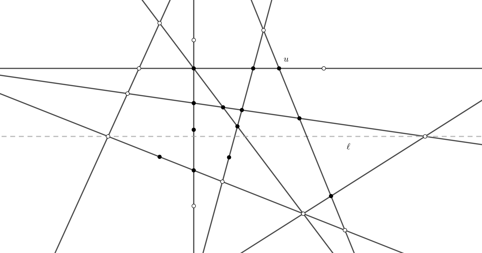
Figure 5. In black the vertices in $S$ and in white those in $V\setminus S$. This figure illustrates a graph $G\in\mathcal{H}$ and the vertex $u$ used in the proof of Theorem 5.

Theorem 5.

If $G\in\mathcal{H}$, then $G$ has the planar shrink property.

Proof.

Given a non-empty subset $S\subset V$ and a straight line $\ell$, suppose without loss of generality that $0<|S_{1}^{\ell}|<\infty$ (see Definition 6). We need to prove that there exists $u\in S_{1}^{\ell}$ such that $deg_{V\setminus S}(u)\geq deg_{S}(u)$. First, we note that by property (P2) every vertex has a degree that is even. Without loss of generality, we can consider the line $\ell$ coincident with the axis $x$ (by applying a translation and a rotation) such that the vertices in $S_{1}^{\ell}$ have a non-negative ordinate. We write every vertex $v\in V$ as $v=(v_{x},v_{y})\in\mathbb{R}^{2}$ and let $r_{y}:=\max_{v\in S_{1}^{\ell}}v_{y}$ and $r_{x}:=\max\{v_{x}\in\mathbb{R}:(v_{x},r_{y})\in S_{1}^{\ell}\}$.

We consider the vertex $u=(r_{x},r_{y})\in V$. Given $w=(w_{x},w_{y})\in N_{S}(u)$, there are two cases to consider (see Figure 5). If $w_{y}=r_{y}$ then, by property (P2), there exists a vertex $w^{\prime}=(w^{\prime}_{x},w^{\prime}_{y})\in N_{V\setminus S}(u)$ with $w^{\prime}_{y}=r_{y}$ and $w^{\prime}_{x}>r_{x}$. If instead $w_{y}<r_{y}$ then, by property (P2), there exists a vertex $w^{\prime}\in N_{V\setminus S}(u)$ with $w^{\prime}_{y}>r_{y}$. In both cases, $w^{\prime}$ belongs to the linear extension of edge $\{u,w\}$ out of $S$. In other words, it is possible to define an injective function

$$f_{u}\colon w\in N_{S}(u)\mapsto w^{\prime}\in N_{V\setminus S}(u),$$

where the vertices $u$, $w$ and $w^{\prime}$ are aligned. This implies that $deg_{V\setminus S}(u)\geq deg_{S}(u)$. ∎

We note that the shrink property holds even if we replace $\mathcal{H}$ with a class of graphs embedded in $\mathbb{R}^{d}$ having the properties (P1), (P2) and (P3), i.e. they are obtained by intersection of lines. The proof of this fact is analogous to the proof of Theorem 5.

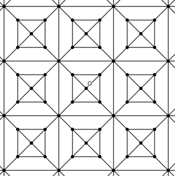
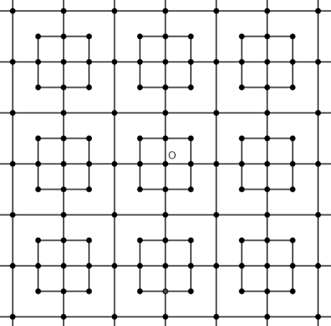
Figure 6. Examples of graphs in $\mathcal{G}(4)$ that do not have the shrink property.

Now, we provide some explicit examples. The square lattice $\mathbb{Z}^{2}$, the triangular lattice (see Figure 7) and the graphs in Figures 1, 7, 8 and 9 belong to class $\mathcal{H}$ therefore, by Theorem 5, all these graphs have the planar shrink property. In particular, we note that the graph on the right in Figure 7 belongs to $\mathcal{G}(3)\setminus\mathcal{G}(6)$, i.e. it is invariant under rotation of an angle of $2\pi/3$, but not of $\pi/3$. In Figure 6 we give two examples of graphs that do not have the shrink property. In Figure 9 we show a graph $G$ with infinite classes that is invariant by a rotation of $\pi$ but not invariant under a rotation of $\pi/2$. For this $I(G,1/2)$-model we can not apply Theorem 4 but we have a proof showing that it is of type $\mathcal{I}$. We do not present this proof that would break the unitary character of our presentation.

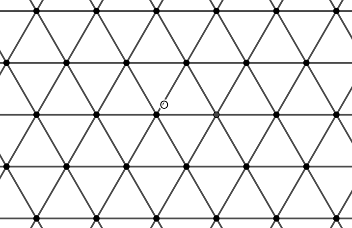
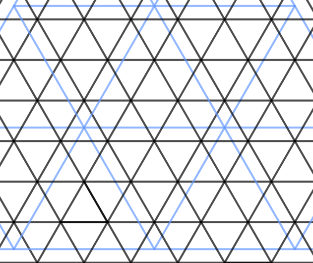
Figure 7. On the left the triangular lattice, example of a graph $G\in\mathcal{G}(6)\cap\mathcal{H}$. On the right a double triangular lattice, example of a graph $G\in(\mathcal{G}(3)\setminus\mathcal{G}(6))\cap\mathcal{H}$.

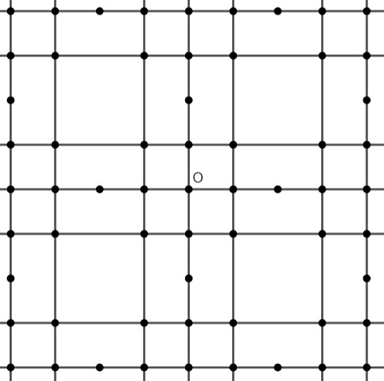
Figure 8. Modified double lattice $\mathbb{Z}^{2}$: example of a graph $G\in\mathcal{G}(4)\cap\mathcal{H}$.

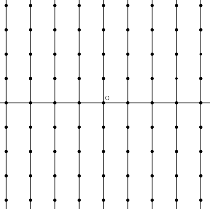
Figure 9. Example of a graph $G\in\mathcal{H}$ that is invariant under translation and rotation of $\pi$, but not of $\pi/2$. The number of classes of $G$ is infinite.

Data Availibility Statement

This mathematical article has no external data to present.

Competing Interests

The authors have no conflicts of interest to declare that are relevant to the content of this article.

Acknowledgements

We thank Andrea Maffei for a useful discussion and comments about Lemma 3.

References

- [1] R. Arratia. Site recurrence for annihilating random walks on . Ann. Probab., 11(3):706–713, 1983.
- [2] I. Benjamini and O. Schramm. Percolation beyond , many questions and a few answers [mr1423907]. In Selected works of Oded Schramm. Volume 1, 2, Sel. Works Probab. Stat., pages 679–690. Springer, New York, 2011.
- [3] R. M. Burton and M. Keane. Density and uniqueness in percolation. Comm. Math. Phys., 121(3):501–505, 1989.
- [4] F. Camia, E. De Santis, and C. M. Newman. Clusters and recurrence in the two-dimensional zero-temperature stochastic Ising model. Ann. Appl. Probab., 12(2):565–580, 2002.
- [5] F. Camia, C. M. Newman, and V. Sidoravicius. Approach to fixation for zero-temperature stochastic Ising models on the hexagonal lattice. In In and out of equilibrium (Mambucaba, 2000), volume 51 of Progr. Probab., pages 163–183. Birkhäuser Boston, Boston, MA, 2002.
- [6] P. Caputo and F. Martinelli. Phase ordering after a deep quench: the stochastic Ising and hard core gas models on a tree. Probab. Theory Related Fields, 136(1):37–80, 2006.
- [7] R. Cerqueti and E. De Santis. Stochastic Ising model with flipping sets of spins and fast decreasing temperature. Ann. Inst. Henri Poincaré Probab. Stat., 54(2):757–789, 2018.
- [8] D. Chelkak, D. Cimasoni, and A. Kassel. Revisiting the combinatorics of the 2D Ising model. Ann. Inst. Henri Poincaré D, 4(3):309–385, 2017.
- [9] M. Damron, S. M. Eckner, H. Kogan, C. M. Newman, and V. Sidoravicius. Coarsening dynamics on with frozen vertices. J. Stat. Phys., 160(1):60–72, 2015.
- [10] M. Damron, H. Kogan, C. M. Newman, and V. Sidoravicius. Fixation for coarsening dynamics in 2D slabs. Electron. J. Probab., 18:No. 105, 20, 2013.
- [11] M. Damron, H. Kogan, C. M. Newman, and V. Sidoravicius. Coarsening with a frozen vertex. Electron. Commun. Probab., 21:Paper No. 9, 4, 2016.
- [12] E. De Santis and A. Maffei. Perfect simulation for the infinite random cluster model, Ising and Potts models at low or high temperature. Probab. Theory Related Fields, 164(1-2):109–131, 2016.
- [13] E. De Santis and C. M. Newman. Convergence in energy-lowering (disordered) stochastic spin systems. J. Statist. Phys., 110(1-2):431–442, 2003.
- [14] R. Diestel. Graph theory, volume 173 of Graduate Texts in Mathematics. Springer, Berlin, fifth edition, 2017.
- [15] S. M. Eckner and C. M. Newman. Fixation to consensus on tree-related graphs. ALEA Lat. Am. J. Probab. Math. Stat., 12(1):357–374, 2015.
- [16] L. R. Fontes, R. H. Schonmann, and V. Sidoravicius. Stretched exponential fixation in stochastic Ising models at zero temperature. Comm. Math. Phys., 228(3):495–518, 2002.
- [17] A. Gandolfi, C. M. Newman, and D. L. Stein. Zero-temperature dynamics of spin glasses and related models. Comm. Math. Phys., 214(2):373–387, 2000.
- [18] R. Gheissari, C. M. Newman, and D. L. Stein. Zero-temperature dynamics in the dilute Curie-Weiss model. J. Stat. Phys., 172(4):1009–1028, 2018.
- [19] O. Häggström and J. Jonasson. Uniqueness and non-uniqueness in percolation theory. Probab. Surv., 3:289–344, 2006.
- [20] T. E. Harris. Contact interactions on a lattice. Ann. Probability, 2:969–988,1974.
- [21] T. E. Harris. A correlation inequality for Markov processes in partially ordered state spaces. Ann. Probability, 5(3):451–454, 1977.
- [22] T. E. Harris. Additive set-valued Markov processes and graphical methods. Ann. Probability, 6(3):355–378, 1978.
- [23] N. Lanchier. Stochastic modeling. Universitext. Springer, Cham, 2017.
- [24] T. M. Liggett. Interacting particle systems, volume 276 of Grundlehren der mathematischen Wissenschaften [Fundamental Principles of Mathematical Sciences]. Springer-Verlag, New York, 1985.
- [25] F. Martinelli. Lectures on Glauber dynamics for discrete spin models. In Lectures on probability theory and statistics (Saint-Flour, 1997), volume 1717 of Lecture Notes in Math., pages 93–191. Springer, Berlin, 1999.
- [26] R. Morris. Zero-temperature Glauber dynamics on . Probab. Theory Related Fields, 149(3-4):417–434, 2011.
- [27] S. Nanda, C. M. Newman, and D. L. Stein. Dynamics of Ising spin systems at zero temperature. In On Dobrushin’s way. From probability theory to statistical physics, volume 198 of Amer. Math. Soc. Transl. Ser. 2, pages 183–194. Amer. Math. Soc., Providence, RI, 2000.
- [28] D. Williams. Probability with martingales. Cambridge Mathematical Textbooks. Cambridge University Press, Cambridge, 1991.