Efficient Sobolev approximation of linear parabolic PDEs
in high dimensions
Abstract
In this paper, we study the error in first order Sobolev norm in the approximation of solutions to linear parabolic PDEs. We use a Monte Carlo Euler scheme obtained from combining the Feynman–Kac representation with a Euler discretization of the underlying stochastic process. We derive approximation rates depending on the time-discretization, the number of Monte Carlo simulations, and the dimension. In particular, we show that the Monte Carlo Euler scheme breaks the curse of dimensionality with respect to the first order Sobolev norm. Our argument is based on new estimates on the weak error of the Euler approximation of a diffusion process together with its derivative with respect to the initial condition. As a consequence, we obtain that neural networks are able to approximate solutions of linear parabolic PDEs in first order Sobolev norm without the curse of dimensionality if the coefficients of the PDEs admit an efficient approximation with neural networks.
1. Introduction
We consider the following linear parabolic partial differential equation (PDE);
| (1.1) |
There is an abundance of results that study numerical approximations of solutions of PDEs of the form (1.1). In physics, engineering, or finance, such equations can appear in very high dimensions. Therefore, it is important whether numerical approximations are affected by the curse of dimensionality, meaning that the complexity of a numerical scheme grows exponentially in the dimension , rendering it unfeasible in such applications. Furthermore, in many cases, a good approximation of the gradient is just as important as a good approximation of the solution . For instance, if is the value of a financial contract, describes the sensitivities, which are intimately related to the optimal hedging strategy.
Suppose the complexity of a numerical approximation of is given by some parameter . Typical error estimates are of the form for some constants . The notion ‘curse of dimensionality’ is not used consistently in the literature and depends on the application. Here, we call free of the curse of dimensionality if does not depend on the dimension and if the constant grows at most polynomially in the dimension.
Numerical simulations have empirically verified the ability to approximate PDEs without the curse of dimensionality, particularly machine learning paradigms; [6, 2, 12, 20]. There is an ever-growing number of articles backing these simulations with proofs for breaking the curse of dimensionality; the reader may consult [4, 11, 12, 13, 14, 24, 27] and the references therein for a comprehensive overview. Almost all of these results measure the error in an -norm (we comment on exceptions later). However, in the context of PDEs, it would be more natural to also study the error incurred by derivatives. In general, a good approximation of in does not have to be a good approximation in Sobolev spaces. In applications, approximations in Sobolev spaces are more desired. Recently, training algorithms for machine learning paradigms have been adapted to incorporate ‘Sobolev training’; [19, 20, 30, 33, 34, 35, 37]. In this Sobolev training, an algorithm takes into account loss values of the derivative approximation of a model; [8, 9, 26]. Physically inspired neural networks are trained so that they satisfy a given PDE as well as possible; [11, 32]. In this approach, derivatives are trained implicitly. In terms of approximation capacities, the theoretical justification for these algorithms is insufficient. They are mainly based on the ability of a model class to admit suitable approximations of a target function in Sobolev space; [1, 10, 15, 16, 17, 31, 32]. But these are usually not quantitative or at least suffer the curse of dimensionality (we comment on exceptions later). In this article, we improve the theoretical justification for the Sobolev training of PDEs by proving error rates for approximating and its first derivative without the curse of dimensionality.
A common approach for approximating solutions to linear parabolic PDEs is to exploit the Feynman–Kac formula and move the approximation problem to the realm of stochastic processes. For a simpler presentation, we here assume but treat non-zero later. Omitting technical assumptions, the Feynman–Kac formula states that
| (1.2) |
where is the solution to PDE (1.1) and is the solution to the corresponding stochastic differential equation (SDE);
| (1.3) |
where is a standard -dimensional Brownian motion. The functions and are called drift and diffusion coefficient, respectively. The expected value in the Feynman–Kac formula can be tackled with a Monte Carlo simulation, which is famously known not to suffer the curse of dimensionality. Thus, the problem reduces to efficiently approximating the stochastic process . Many numerical schemes have been studied for this purpose, the most prominent one being the Euler scheme and variations of it. Fix a deterministic time grid . The explicit Euler scheme in its standard form is given by
| (1.4) |
We now state an informal version of our main result.
Theorem 1.1 (informal).
Let , , , , and adhere to certain regularity assumptions, where is a solution to PDE (1.1). Let be independent copies of the Euler scheme (1.4) for SDE (1.3) based on a uniform time grid with steps. Consider given by
| (1.5) |
In the following, denotes a constant that depends only on and , and denotes a constant that depends on , , , , , , and . Now, the probabilistic numerical scheme approximates the PDE solution at time 0 in the following sense. Let and let be compact. If , then
provided and are so large that
The regularity assumptions required and the constants and will be made explicit in our main result, Theorem 3.10. We remark that these constants can depend implicitly on the dimension since the functions , , , , and do. The specification in Theorem 3.10 unfolds this implicit dependence, linking it to the spatial growth of the functions. In particular, it reveals in which case the curse of dimensionality is broken to the full extent. Additionally, we will argue why we cannot expect to alleviate the implicit dependence. Let us mention that starting the Euler scheme at time is convenient for the sake of notation. But if we let it start at an arbitrary initial time and define the Euler scheme on the uniform time grid in , then we obtain a time-dependent that approximates in the norm at an analogous rate.
There is a vast amount of results on convergence properties and error rates of the Euler scheme. We summarize the findings most relevant to us here but refer to the exposition in [5, 22] and the references [29, 3, 5, 28, 21, 18] for a more detailed account of the existing literature. Typically, to obtain not only mere convergence but also a rate of convergence, assumptions imposed on the drift and diffusion coefficients involve global Lipschitz continuity in the space variable and Hölder continuity in the time variable. To relax the global Lipschitz continuity for both coefficients simultaneously, [36] instead imposed on them to grow at most linearly and be locally Lipschitz continuous with local Lipschitz constants on balls growing at most logarithmically in the diameter. The first of these assumptions is sharp in the following sense: [22, 23] showed that the Euler scheme diverges as soon as one of the coefficient functions grows more than linearly. In this article, we narrow the gap to the negative results in [22, 23] by proving a convergence rate for the Euler scheme for at most linearly growing coefficients with a much weaker growth assumption on the local Lipschitz constants than in [36]. Our result, Theorem 2.8, is based on a weak error estimate, which is the reason for the regularity requirements in Theorem 1.1.
Let us illustrate in more detail our method of attack to obtain Sobolev approximations of PDE (1.1) based on the Feynman–Kac formula. A key observation is the well-known differentiability of the stochastic process and its Euler scheme with respect to the initial point . From the Feynman–Kac formula (1.2), it is to be expected that
| (1.6) |
The derivative of the Euler scheme is given by
We cannot apply known error estimates for Euler schemes to because is not the Euler scheme of . Nonetheless, we can regard as a Euler scheme by considering it simultaneously with . Indeed, the Euler scheme of the combined process is exactly . The combined process solves the SDE with the new drift coefficient and diffusion coefficient . Now that we can view as a Euler scheme, we can tackle the error estimate in (1.6). The existing tools surveyed above are not applicable to the coefficients and , but we will be able to apply the new convergence rate result from this article.
Let us mention a special case, in which Sobolev approximation of PDEs free of the curse of dimensionality has been achieved. This has been done for the heat equation in [4] and, more generally, for the PDE (1.1) under the assumption that and are affine functions of in [11]. The key to this result is that the stochastic process itself becomes an affine function of and the approximation error can be estimated with a simple Monte Carlo argument. More precisely, there exist random variables and independent of such that . Then, there exist matrices and vectors such that (1.6) simplifies to
In this article, we extend the findings of [4, 11] to non-affine coefficients. Lastly, we present an application to the approximation theory of neural networks. Networks have also been employed in [4, 11], among other works mentioned above. This is due to the compositional structure of networks, which makes them suitable to implement the Monte Carlo Euler scheme from Theorem 1.1. If the coefficients and and the functions and can be represented by networks, then the function given in (1.5) can also be represented by a network element-wise for each . This gives rise to a network Sobolev approximation of the solution to PDE (1.1). If the coefficients cannot be represented exactly, then we approximate them with networks and build an analogous function , where , , , and are replaced by their network approximations. This yields a perturbed scheme, for which we derive corresponding error estimates. To obtain a network approximation that breaks the curse of dimensionality, we require the approximations of the coefficients to be efficient. This is done in Theorem 4.8. As such, we provide the first proof that networks can approximate solutions to PDEs with non-affine coefficients in a Sobolev sense without the curse of dimensionality.
Our exposition is structured as follows. We prove the new weak error rate of the Euler scheme for at most linearly growing coefficients in Section 2. Thereafter, we add a global Lipschitz assumption on the coefficients to obtain a rate of convergence in the first order Sobolev norm. The perturbed scheme is analyzed in Section 4, first in general and then for networks. In the appendix, we develop the technical ‘polynomial growth calculus’, which proves useful for keeping track of implicit dependencies of constants on the dimension.
Notation
Euclidean spaces are endowed with the Frobenius norm . Throughout, we fix a time horizon , measurable drift and diffusion coefficients and , the inhomogeneity of the PDE , and the terminal value of the PDE . We let be the operator acting on twice differentiable functions by222We understand as the -dimensional vector with elements , , for .
For a time-dependent function , we write . Then, with the operator given by
we can write PDE (1.1) succinctly as . We call the generator.
For the stochastic part, we work on a complete probability space with a filtration satisfying the usual conditions and a standard -valued Wiener process for . The norm on , , will be denoted by . We let be the Banach space of all -adapted -a.s. continuous -valued stochastic processes on with norm
Let be the subset .
2. Weak error rate for the Monte Carlo Euler scheme
2.1 Measuring polynomial growth
As discussed in the introduction, breaking the curse of dimensionality in an approximation task involves polynomial control on the constant in the error estimate with respect to the dimension. Any reasonable numerical scheme for approximating solutions of PDEs of the form (1.1) and with it its error estimate will in one way or another depend on the drift and diffusion coefficients. The spatial domain of and is , which unveils an implicit dependence on the dimension. Thus, we need to quantify how the approximation error depends on and to guarantee that this implicit dependence does not incur the curse of dimensionality. We approach this with measuring the polynomial growth of a function. Since we study Sobolev approximations and will rely on a weak error estimate for the Euler scheme, we consider the growth of derivatives.
Definition 2.1.
For a -times differentiable function and , we introduce the growth measure
If depends on time, then we let . Since will appear frequently, we shorten this to
Example 2.2.
Let be Lipschitz continuous with Lipschitz constant . Then, for all ,
If, in addition, is differentiable, then, for all ,
We remark that if , then ; see Lemma A.1 in the appendix. The converse is obvious. The exact definition of with the power in the denominator is for convenience, because it allows for concise inequalities such as the following.
Lemma 2.3.
Let be -times differentiable and . Then, for any with , we have
Proof.
This is immediate from a change of summation index in the definition of . ∎
We will require the drift and diffusion coefficients to be Hölder continuous in time, but allow the Hölder constant to grow in space.
Definition 2.4.
For a function and , , we introduce the Hölder growth measure
The reason for introducing these growth measures is to develop a ‘polynomial growth calculus’, with which we can conveniently estimate the growth of a function by that of related functions without knowing anything else about those other functions. An example of this was given in Lemma 2.3. Another example, which we will use later, is the following estimate for the growth of the generator applied to a function twice. To state this example, it is convenient to introduce the operators and acting on twice differentiable functions by
Lemma 2.5.
Assume and are twice differentiable in the space variable and let .
-
(i)
For any twice differentiable function and any ,
(2.1) with .
-
(ii)
For any four times differentiable function and any ,
with , and the same bound holds for .
Estimate (2.1) also holds for and in place of and for a function with domain , since we can apply the lemma with . The proof of Lemma 2.5 is deferred to the appendix, in which we develop a more elaborate ‘polynomial growth calculus’.
There is one particular cumbersome constant that will appear in several of the results to come. To avoid repeating it throughout, we introduce it here as
| (2.2) |
2.2 Weak error rate for the Euler scheme
The Euler scheme is usually regarded as a temporal discretization of an SDE. However, for a weak error analysis, one can introduce the Euler scheme directly without considering the original SDE. Fix a natural number and abbreviate . Given , we write for , . Then, for any , we let be the Euler scheme
Here, we take as the initial time to keep the notation simple, but all arguments go through for an arbitrary initial time . It is not difficult to show that the Euler scheme is an element of if for some . In the lemma below, we derive a bound on in the case of at most linearly growing and , that is . The qualitative version of this lemma is well-known but we need a quantitative version with explicit constants.
Lemma 2.6.
Let and . If , then there exists a constant that depends only on such that for all
Proof.
Throughout, denotes a constant that depends only on but may change from line to line. Abbreviate . By Itô’s formula applied to the function , we have
| (2.3) |
For any ,
Thus, by Hölder’s inequality,
| (2.4) |
For each and , we can apply Doob’s maximal inequality to the martingale indexed by to find
Hence, if , then
The estimate in (2.4) simplifies to . We plug this into (2.3);
Finally, by Grönwall’s inequality, . ∎
We have laid the groundwork for our weak error analysis of the Euler scheme in the approximation of PDE solutions. The following smoothness assumptions are needed to apply Itô’s lemma in the proof of Theorem 2.8.
Assumption 2.7.
Suppose , , and are twice continuously differentiable in the space variable, is also continuously differentiable in the time variable, and is four times continuously differentiable. Suppose solves the PDE
We remark that growth assumptions on and that guarantee everything to be well-posed are implicit. For if such growth assumptions were not met, then the bound in the theorem below and in the other results to come would have infinity on the right hand side and the statement of the theorem would become void.
Theorem 2.8.
Let Assumption 2.7 hold and consider given by
Let , , and denote and ; see (2.2). If , then there exists a constant depending only on such that for all
Proof.
Abbreviate . Since , we have
By Itô’s formula and the PDE solved by ,
From now on, we write
so that . We first bound , which we split into the three terms
We can apply Itô’s formula to for each to rewrite as
In the estimates to come, denotes a constant that depends only on but may change from line to line. By Lemma 2.5,
where . Note that . Thus,
We can also apply Itô’s formula to rewrite as
By Lemma 2.5, we obtain the same bound for as for (up to adjusting ). We can estimate by
Furthermore, using the (Hölder) growth measure and the equality ,
By Lemma 2.3, . Similarly,
Therefore,
where . Combining the bounds for , , and , we find the following bound for ;
Next, we bound , which we can write as . By Itô’s formula,
By Lemmas 2.3 and 2.5,
Thus,
where . Combining the bounds for and , we have shown
where . By Lemma 2.6, if , then
This yields the final bound
∎
In Theorem 2.8, we see that the error rate is free of the curse of dimensionality as long as we can reasonably control the constants and . On the one hand, appears as a multiplicative factor in the bound and, hence, should grow at most polynomially in the dimension. On the other hand, appears as an exponent and, hence, and should grow at most logarithmically in the dimension. The fact that we have to control these constants is intuitive: if any of the involved functions itself grows exponentially in the dimension, then we cannot expect the discrete Euler scheme to explore all relevant regions with a time grid whose fineness is polynomial in the dimension.
2.3 Monte Carlo estimates
To obtain a numerical scheme from the Feynman–Kac formula, we approximate the expected value with a Monte Carlo method. The Monte Carlo method is famously known to break the curse of dimensionality. However, this folklore suppresses the variance of the integrand appearing in the Monte Carlo estimate. Therein can appear an implicit dependence on the dimension and, hence, may still incur the curse. We present an estimate of the Monte Carlo method based on the polynomial growth measure to quantify the implicit dependence.
Proposition 2.9.
Let be independent copies of . Consider and given by
Let , , let be a compact set, and denote and . If , then there exists a constant , depending only on , such that
provided is so large that
Proof.
We use a standard argument for bounding Monte Carlo errors. First, by Markov’s inequality,
Secondly,
By Jensen’s inequality,
As in the previous proofs, denotes a constant that depends only on but may change form line to line. We use the bound and similarly for to find
By Lemma 2.6, if , then
Thus,
∎
By combining the error analysis for the Euler scheme and the Monte Carlo method, we find the following rate of convergence for the Monte Carlo Euler scheme.
Corollary 2.10.
Let Assumption 2.7 hold and let be independent copies of . Consider given by
Let , , , let be compact, and denote and ; see (2.2). If , then there exists a constant , depending only on , such that
provided and are so large that
Proof.
This is immediate from Theorems 2.8 and 2.9. ∎
As before, we see that the error rate for the Monte Carlo Euler scheme is free of the curse of dimensionality as long as we can control and . The same comment we made after the proof of Theorem 2.8 applies here. An implementation of this scheme requires independent simulations of a standard -dimensional normal random vector.
Remark 2.11.
If we consider the Euler scheme starting at time instead of at time 0, that is setting and defining
then the Monte Carlo Euler scheme in Corollary 2.10 becomes a time-dependent approximation with
provided and are so large that
To implement the time-dependent scheme, independent simulations of a -dimensional normal random vector are still sufficient because we do not need the simulations of to be independent for different , so we can use simulations of with the same for each .
This concludes the discussion about the numerical scheme for approximating PDE (1.1) in . In the next section, we will set the stage to obtain Sobolev approximations of the PDE.
3. Numerical Sobolev approximation of PDE solutions
3.1 Augmented derivatives of PDEs
In the introduction, we motivated considering the combined process , where solves SDE (1.3). The combined process solves another SDE, namely with the drift coefficient and diffusion coefficient . In light of this, it becomes natural to introduce the following terminology of an augmented derivative. This terminology is chiefly a matter of notation, which will enable us to rewrite the problem of obtaining Sobolev approximations of PDE (1.1) so as to fit the setting of the previous section.
Definition 3.1 (Augmented derivative).
Given a Fréchet differentiable function between two Banach spaces, whose Fréchet derivative at a point is denoted , , we let be the function
If the function is time-dependent, then we denote .
The augmented derivative augments the derivative with the original function. Note that it is linear in and satisfies the chain rule . The convenience of the augmented derivative in terms of notation is demonstrated in the next result. In general, the standard derivative does not satisfy . This equality becomes true when we replace the standard derivative by the augmented derivative. We briefly omit the time-dependence of and for increased readability.
Proposition 3.2 (Commutativity of augmented derivatives and generators).
Suppose and are differentiable in the space variable and is three times differentiable. Let be given by . Then and .
Proof.
On the one hand, we calculate
and
On the other hand,
Thus, . Lastly, let and be given by and , respectively. Then and . In particular, by the chain rule for the augmented derivative,
∎
As an immediate consequence of the previous result, we find that the augmented derivative of a solution to PDE (1.1) solves the augmented derivative of the PDE, meaning the PDE whose coefficients are the augmented derivatives of the original coefficients.
Corollary 3.3 (Commutativity of augmented derivatives and PDEs).
Suppose , , and are differentiable in the space variable, and solves the PDE . Then, solves the PDE .
Proof.
This is an immediate consequence of Proposition 3.2. ∎
In the next section, we will see that the augmented derivative interacts as nicely with SDEs as with PDEs.
3.2 Augmented derivatives of Euler schemes
Consider the SDE
| (3.1) |
with initial condition . It is a classical result that this SDE admits a unique solution under certain regularity assumptions on and . Under stronger regularity assumptions on the coefficients, the solution map , becomes differentiable; [25]. In particular, we can take its augmented derivative. The augmented derivative of a Fréchet differentiable map is a map . We can identify the product with the space . This identification works on the the level of Banach spaces because the norm on is equivalent to the norm on . Henceforth, we regard the augmented derivative of a map as taking values in .
Assumption 3.4.
Suppose and are continuous in time and continuously differentiable in space such that their spatial derivatives are globally bounded uniformly in time.
Proposition 3.5 (Commutativity of augmented derivatives and SDEs).
Let Assumption 3.4 hold. Then, for any , the function is Fréchet differentiable and . In particular, maps into and is independent of .
Proof.
This is proved in [25], only rephrased in the language of augmented derivatives. ∎
Naturally, the same assumptions on the coefficients that guaranteed differentiability of provide the same regularity for the Euler scheme. Again, this is conveniently formulated with the help of augmented derivatives. For a moment, we make the dependence of the Euler scheme on the coefficient functions explicit and write .
Proposition 3.6 (Commutativity of augmented derivatives and Euler schemes).
Let Assumption 3.4 hold. Then, for any , the function is Fréchet differentiable and . In particular, maps into and is independent of .
Proof.
By Assumption 3.4, the functions and are Lipschitz continuous with a Lipschitz constant independent of time. This implies that and grow at most linearly in the space variable. In particular, Lemma 2.6 and its proof assert that the Euler scheme for the functions and is indeed an element of . For any , let be the second component of , that is
Fix . We show that is the Fréchet derivative of at applied to . In this proof, there is no need to track constants explicitly. Henceforth, denotes a constant that may change from line to line but always stays independent of and . Abbreviate
Our goal is to show that . Using the recursive structure of the Euler scheme, we see that
To the last term, we can apply the Burkholder–Davis–Gundy inequality to find
Let us write
so that uniformly
Using that is Lipschitz continuous, we estimate
We proceed analogously for the term involving . Thus,
| (3.2) |
where we used Hölder’s inequality in the second line. Now, abbreviate
Similarly as for , by the Burkholder-Davis-Gundy inequality and Lipschitz continuity, . In particular, . Iterating the recursion in (3.2), we find
The limit of as exists pointwise and equals 0. Furthermore, the Lipschitz continuity of and implies that is uniformly bounded. Hence, we can apply dominated convergence to find
This concludes Fréchet differentiability of with the correct derivative if we show that is a bounded linear operator in . Boundedness was shown implicitly in the previous calculations. Indeed, by Jensen’s inequality,
and this is bounded uniformly in because is. For linearity, abbreviate
As for , by the Burkholder–Davis–Gundy inequality and the Lipschitz continuity of and , we obtain . ∎
The final preparation for the Sobolev approximation is a standard argument for interchanging expectation and differentiation.
Lemma 3.7.
Let Assumption 3.4 hold and suppose and are continuously differentiable in space with for some . Then, the function given by
is differentiable and its augmented derivative is
Proof.
Let us write for the Fréchet derivative of and
We will show differentiability of the map . The argument for is completely analogous. We begin with the estimate
By Hölder’s inequality and the definition of ,
The expectation of is finite since and for some . As in the proof of Proposition 3.6, we find for some constant independent of and . Thus, differentiability of implies
To this term, we can apply dominated convergence because and
for some (other) constant independent of and . We have seen in the proof of Proposition 3.6 that and, hence, is a bounded linear map in . ∎
3.3 Sobolev error rate for the Monte Carlo Euler scheme
In this section, we prove the error rate for the Sobolev approximation of PDE (1.1). The results of the previous section enable us to directly apply the weak error rate of the Euler scheme and the Monte Carlo estimate to in place of . Since the augmented derivatives of all functions involved have to satisfy the assumptions of Theorem 2.8, we need to upgrade Assumption 2.7 to one more order of differentiability.
Assumption 3.8.
Let Assumption 3.4 hold and suppose , , and are three times continuously differentiable in the space variable, is also continuously differentiable in the time variable, and is five times continuously differentiable. Suppose solves the PDE
With these assumptions in place, Theorem 2.8 can be upgraded immediately to yield an analogous error bound for . Likewise, by applying Corollary 2.10 to the augmented derivatives of the PDE solution and its Monte Carlo Euler approximation , we find a result of the form
for any compact and sufficiently large and . If , then the error is given by
In particular, it involves the integral . This is not how the error of the derivative is usually measured. Instead, we would like to measure in the Frobenius norm. Converting the former measure of error to the latter can be done as follows.
Lemma 3.9.
Let be differentiable. Then, for all ,
where is the Euclidean -dimensional ball of radius 1 centered at the origin and is the Gamma function .
Proof.
Take with unit norm such that equals the operator norm of . Let be the orthogonal complement of in with respect to the standard inner product. Then, for any and ,
Let for some fixed . Then,
where we used that by symmetry of the ball . Thus,
The integral is the volume of half of a -dimensional ball of radius , so
Finally, because the rank of can be at most . ∎
Now, we can deduce the main result of this article about the Sobolev approximation of PDE (1.1) with a Monte Carlo Euler scheme.
Theorem 3.10.
Let Assumption 3.8 hold and let be independent copies of . Consider given by
Let , , , let be compact, and denote and ; see (2.2). If , then there exists a constant , depending only on , such that
provided and are so large that
Proof.
Let be the -dimensional Euclidean ball of radius 1 centered at the origin. As usual, denotes a constant that depends only on but may change from line to line. Observe that are independent copies of . We apply Corollary 2.10, which is possible by Corollaries 3.3, 3.6, and 3.7, to find
provided and are so large that and
Now, by Lemma 3.9,
and, trivially,
Hence,
Then,
provided and are so large that
Abbreviating and using that , we find
Moreover,
Thus,
where we used that . We conclude that a sufficient bound for and is
∎
Remark 3.11.
As in Remark 2.11, if we consider the Euler scheme starting at time , then we obtain a time-dependent approximation with
provided and are so large that
As in Corollary 2.10, the curse of dimensionality is broken if grows at most polynomially in the dimension and at most logarithmically. This time, these constants measure the spatial growth of the augmented derivatives of the coefficients. To give an example of how might behave, we revisit Example 2.2.
Example 3.12.
Let be differentiable and Lipschitz continuous with Lipschitz constant . Then, for all ,
Thus, if the Lipschitz constant of and grows at most logarithmically in the dimension, then the constant in Theorem 3.10 grows at most polynomially in the dimension. Some more specific examples are as follows.
Example 3.13.
Let , , be differentiable and Lipschitz continuous with Lipschitz constant .
-
(i)
Consider the function given by . Then, for all ,
-
(ii)
Consider the function given by and suppose for all . Then, for all ,
4. Monte Carlo Euler scheme with perturbed coefficients
4.1 Error rate for the perturbed scheme
In the previous two sections, we derived (Sobolev) error rates for the Monte Carlo Euler scheme. The next step is to perturb the coefficients and and the functions and and see how the resulting scheme performs. First, we analyze growth and Lipschitz properties of the Euler scheme, jointly in the initial condition and the coefficients. In Lemma 2.6, we considered the norm of the Euler scheme as a stochastic process. In the lemma below, we consider its Euclidean norm point-wise. Throughout this section, and denote functions and and denote measurable functions, which we think of as perturbations of , , , and .
Lemma 4.1.
Denote and . Then, the following hold.
-
(i)
We have, almost surely for all and ,
(4.1) -
(ii)
If, in addition, and are differentiable in the space variable, then, almost surely for all and ,
(4.2) where and .
Proof.
Fix and abbreviate and . We first show (4.1). To this end, observe that and likewise for . The recursion
translates into the bound
With , we immediately deduce (4.1). The inequality (4.2) is shown similarly once we note that
and
Analogous bounds hold for and . Plugging this into the recursion defining and and abbreviating and , we find
Since , expanding this recursion yields
We proved in (4.1) that , with which we conclude
∎
We translate the bound from the previous lemma into the expectation appearing in the Feynman–Kac formula. Then, we will apply Monte Carlo sampling to the expectation in the function specified below instead of to the expectation in as done previously.
Proposition 4.2.
Assume , , , , , and are differentiable in the space variable. Consider and given by
Denote
If , then, for all ,
Proof.
Now, we immediately obtain the error estimate for the perturbed Monte Carlo Euler scheme.
Corollary 4.3.
Let Assumption 2.7 hold and suppose , , , and are differentiable in the space variable. Let be independent copies of . Consider given by
Let , , , let be compact, and denote
see (2.2). If and , then there exists a constant , depending only on , such that
provided and are so large that
and is so small that
Proof.
This is immediate from Theorems 2.8, 2.9, and 4.2 (we apply Proposition 2.9 with to the Euler scheme with coefficients and and to the functions and ). ∎
We see in Corollary 4.3 that the requirement on and is verbatim from Corollary 2.10. In particular, this does not incur the curse of dimensionality if we can control and . However, this is not true for the requirement on , which scales exponentially in . The error inferred from perturbing the coefficients is harder to control than the error from the Monte Carlo Euler scheme itself. As such, the perturbed scheme is provably useful only if the cost of the perturbations in a numerical sense is exponentially small.
4.2 Sobolev error rate for the perturbed scheme
As with Theorem 3.10, the Sobolev error rate for the perturbed Monte Carlo Euler scheme is obtained by applying Corollary 4.3 to the augmented derivatives and using the trick from Lemma 3.9. In particular, we need to impose one more order of regularity on all functions involved.
Assumption 4.4.
Let Assumption 3.8 hold and suppose , , , and are twice differentiable in the space variable. Suppose that and also satisfy Assumption 3.4.
Theorem 4.5.
Let Assumption 4.4 hold and let be independent copies of . Consider given by
Let , , , let be compact, and denote
see (2.2). If and , then there exists a constant , depending only on , such that
provided and are so large that
and is so small that
Proof.
We deduce this from Corollary 4.3 the same way we deduced Theorem 3.10 from Corollary 2.10 with the additional analogous computation
The requirement on and to satisfy Assumption 3.4 ensures that commutes with the augmented derivative by Proposition 3.6. ∎
4.3 Neural network approximations
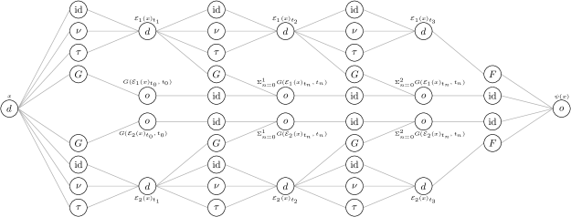
We mentioned in the introduction that neural networks are particularly handy since their compositional structure makes them well-suited to imitate the Monte Carlo Euler scheme. A network is a concatenation of affine functions and a fixed nonlinearity , which is applied component-wise. We say the network has depth and consists of layers. The tuple of the input, respectively output dimensions of the affine functions comprise the architecture of the network. We allow for identity nodes, meaning that one may also apply the identity function instead of the nonlinearity at any point in the network. The parameters that characterize the affine functions are called the parameters of the network. Let denote the number of non-zero parameters. The next lemma showcases that networks can implement the Monte Carlo Euler scheme efficiently if the coefficients are given by networks. It is straight-forward to prove; see Figure 1 for an illustration of the architecture.
Assumption 4.6.
Suppose, for each fixed , that the functions , , , and are given by networks, whose architectures are independent of and whose depths are all the same, namely .
Lemma 4.7.
Let Assumption 4.6 hold and let be copies of . Then, almost surely for all , the function
can be given by a network with
Finally, we use networks for Sobolev approximations of the PDE solution . To this end, we assume that the coefficients can be efficiently approximated with networks and then use these networks in the perturbed scheme. Theorem 4.5 asserts that there exists an element such that a realization of the perturbed scheme approximates to accuracy . This realization can be implemented by a network as shown in the previous lemma. After Corollary 4.3, we remarked that the cost of the perturbations needs to be exponentially small. This means that the coefficients need to be approximated by the respective networks at an algebraic rate.
Theorem 4.8.
Let Assumptions 4.4 and 4.6 hold. Let , , , and denote
Suppose that the quantities
are all bounded by for a constant depending only on and , and suppose
where is a universal constant and . Then, there exists a constant , depending only on , , , and , and a network such that
and
Proof.
This follows from Theorems 4.5 and 4.7. That it suffices to require polynomial growth in the dimension of as opposed to and et cetera follows from the ability to rid the function in of (augmented) derivatives in exchange for increasing the index and decreasing the index ; see Lemma 2.3 and Lemma A.3 in the appendix. ∎
We saw in Example 3.12 that the Lipschitz constant of and growing at most logarithmically in the dimension is a sufficient criterion to ensure polynomial growth of in the dimension. For the network approximation, we would require the same from and . Fortunately, network approximations of a Lipschitz continuous function can often be asserted to meet the same Lipschitz continuity as the approximated function; [7]. In that case, polynomial growth of in the dimension is guaranteed also in Theorem 4.8. This concludes the first proved Sobolev approximation of solutions to PDE (1.1) with non-affine coefficients by networks free of the curse of dimensionality, up to controlling the constant .
Appendix A Polynomial growth calculus
We develop a ‘polynomial growth calculus’ for the growth measure introduced in Definition 2.1. In particular, we prove Lemma 2.5.
A.1 Polynomial growth of derivatives
The first result shows that if for some , then with the same .
Lemma A.1.
Let be -times differentiable and . Then, for any , we have
Proof.
We claim that
for all . The statement of the lemma is shown by applying this inequality repeatedly. Now, note that
A basic calculus argument shows that
Thus,
from which the claim follows. ∎
The second result interchanges higher-order derivatives and the augmented derivative.
Lemma A.2.
Let be -times differentiable and . Then, for any with , we have
Proof.
We claim for every that is a block-tensor that contains as exactly -many blocks, contains as exactly one block, and all of its remaining blocks are zero. If the claim holds, then, for any ,
which implies the statement of the lemma. The claim is immediate from an inductive argument. The case holds by definition. For , if we differentiate again, we differentiate -many blocks with respect to , which yields -many blocks ; we differentiate the one block with respect to , which yields the -th block ; and we differentiate the one block with respect to , which yields the one block . ∎
Lemma A.1 showed that we can decrease the subscript of by trading derivatives of . Conversely, Lemma A.3 shows that we can integrate by increasing the subscript of and adjusting the power . This lemma is a generalization of Lemma 2.3, which corresponds to the case .
Lemma A.3.
Let be -times differentiable and , . Write for the -fold augmented derivative of . Then, for any with , we have
Proof.
By definition and a shift of summation index, we have
Now, we claim that, for any -times differentiable function and any ,
If this claim holds, then we can apply it repeatedly to find
It remains to verify the claim. The case follows from
For a general , we use Lemma A.2 to estimate
Applying the case to the function yields . By Lemma 2.3, , which concludes the proof of the claim. ∎
When decreasing the subscript of , we can get an alternative to Lemma A.1 by trading augmented derivatives instead of standard derivatives as shown in the next lemma.
Lemma A.4.
Let be -times differentiable and , . Write for the -fold augmented derivative of . Then,
Proof.
If we show that, for any -times differentiable function ,
then the lemma follows from a repeated application of this inequality. The factor arises from the fact that the domain of the -fold augmented derivative of is . Let us consider the case . Since the Frobenius norm of can be bounded by the square root of its rank times its operator norm, we can bound
and, hence,
Thus, . Applying this to , we find, for a general ,
By Lemmas A.2 and A.3, the second term can be further bound by
Finally,
where the first inequality follows from , the second one from Lemma A.3, and the last one from being non-increasing in . ∎
A.2 Polynomial growth of generators
The next lemma is the first part of Lemma 2.5.
Lemma A.5.
Let be twice differentiable and . Then, for any ,
with .
As mentioned after Lemma 2.5, the same estimate also holds for and in place of and for a function with domain , since we can apply the lemma with .
Proof.
It is clear that . Observe that
Thus,
from which the desired inequality follows. ∎
Finally, we fill in the complete proof of Lemma 2.5.
Proof of Lemma 2.5..
As mentioned above, the first part of Lemma 2.5 is precisely Lemma A.5. Now, let us consider the function . By Lemma A.5,
where
By Lemma A.3,
Let , , and be the two fold augmented derivatives of , , and , respectively. Applying first Lemma A.3, then Lemma A.4, and then Proposition 3.2, we obtain
since is the input dimension of . By Lemma A.5,
By Lemma A.3,
and . In conclusion, using that ,
The proof for the function is completely analogous with the only exception being the estimate
since the input dimension of is whereas before we had a factor of . ∎
AcknowledgmentsWe are grateful to Philipp Zimmermann and Robert Crowell for fruitful discussions and helpful comments.
References
- [1] Abdeljawad, A., and Grohs, P. Approximations with deep neural networks in Sobolev time-space. Analysis and Applications 20, 03 (2022), 499–541.
- [2] Beck, C., Becker, S., Grohs, P., Jaafari, N., and Jentzen, A. Solving the Kolmogorov PDE by Means of Deep Learning. Journal of Scientific Computing 88, 3 (Jul 2021), 73.
- [3] Berkaoui, A., Bossy, M., and Diop, A. Euler scheme for SDEs with non-Lipschitz diffusion coefficient: strong convergence. ESAIM: Probability and Statistics 12 (2008), 1–11.
- [4] Berner, J., Dablander, M., and Grohs, P. Numerically Solving Parametric Families of High-Dimensional Kolmogorov Partial Differential Equations via Deep Learning. In Advances in Neural Information Processing Systems (2020), H. Larochelle, M. Ranzato, R. Hadsell, M. Balcan, and H. Lin, Eds., vol. 33, Curran Associates, Inc., pp. 16615–16627.
- [5] Bossy, M., Jabir, J.-F., and Martínez, K. On the weak convergence rate of an exponential Euler scheme for SDEs governed by coefficients with superlinear growth. Bernoulli 27, 1 (2021), 312 – 347.
- [6] Chan-Wai-Nam, Q., Mikael, J., and Warin, X. Machine Learning for Semi Linear PDEs. Journal of Scientific Computing 79, 3SN - 1573-7691 (Jun 2019), 1667–1712.
- [7] Cheridito, P., Jentzen, A., and Rossmannek, F. Efficient Approximation of High-Dimensional Functions With Neural Networks. IEEE Transactions on Neural Networks and Learning Systems 33, 7 (2022), 3079–3093.
- [8] Cocola, J., and Hand, P. Global Convergence of Sobolev Training for Overparameterized Neural Networks. In Machine Learning, Optimization, and Data Science (2020), G. Nicosia, V. Ojha, E. La Malfa, G. Jansen, V. Sciacca, P. Pardalos, G. Giuffrida, and R. Umeton, Eds., Springer International Publishing, pp. 574–586.
- [9] Czarnecki, W. M., Osindero, S., Jaderberg, M., Swirszcz, G., and Pascanu, R. Sobolev Training for Neural Networks. In Advances in Neural Information Processing Systems (2017), I. Guyon, U. V. Luxburg, S. Bengio, H. Wallach, R. Fergus, S. Vishwanathan, and R. Garnett, Eds., vol. 30, Curran Associates, Inc.
- [10] De Ryck, T., Lanthaler, S., and Mishra, S. On the approximation of functions by tanh neural networks. Neural Networks 143 (2021), 732–750.
- [11] De Ryck, T., and Mishra, S. Error analysis for physics informed neural networks (PINNs) approximating Kolmogorov PDEs. arxiv:2106.14473v2 (2021).
- [12] E, W., Han, J., and Jentzen, A. Algorithms for solving high dimensional PDEs: from nonlinear Monte Carlo to machine learning. Nonlinearity 35, 1 (dec 2021), 278.
- [13] Gonon, L., and Schwab, C. Deep ReLU network expression rates for option prices in high-dimensional, exponential Lévy models. Finance and Stochastics 25, 4 (Oct 2021), 615–657.
- [14] Grohs, P., and Herrmann, L. Deep neural network approximation for high-dimensional elliptic PDEs with boundary conditions. IMA Journal of Numerical Analysis 42, 3 (05 2021), 2055–2082.
- [15] Gühring, I., Kutyniok, G., and Petersen, P. Error bounds for approximations with deep ReLU neural networks in Ws,p norms. Analysis and Applications 18, 05 (2020), 803–859.
- [16] Hon, S., and Yang, H. Simultaneous neural network approximation for smooth functions. Neural Networks 154 (2022), 152–164.
- [17] Hornik, K., Stinchcombe, M., and White, H. Universal approximation of an unknown mapping and its derivatives using multilayer feedforward networks. Neural Networks 3, 5 (1990), 551–560.
- [18] Hu, L., Li, X., and Mao, X. Convergence rate and stability of the truncated Euler–Maruyama method for stochastic differential equations. Journal of Computational and Applied Mathematics 337 (2018), 274–289.
- [19] Huge, B., and Savine, A. Differential Machine Learning. arXiv:2005.02347v4 (2020).
- [20] Huré, C., Pham, H., and Warin, X. Deep backward schemes for high-dimensional nonlinear PDEs. Math. Comp. 89, 324 (2020), 1547–1579.
- [21] Hutzenthaler, M., and Jentzen, A. On a perturbation theory and on strong convergence rates for stochastic ordinary and partial differential equations with nonglobally monotone coefficients. The Annals of Probability 48, 1 (2020), 53 – 93.
- [22] Hutzenthaler, M., Jentzen, A., and Kloeden, P. E. Strong and weak divergence in finite time of Euler’s method for stochastic differential equations with non-globally Lipschitz continuous coefficients. Proceedings of the Royal Society A 467 (2011), 1563–1576.
- [23] Hutzenthaler, M., Jentzen, A., and Kloeden, P. E. Divergence of the multilevel Monte Carlo Euler method for nonlinear stochastic differential equations. The Annals of Applied Probability 23, 5 (2013), 1913 – 1966.
- [24] Hutzenthaler, M., Jentzen, A., Kruse, T., and Nguyen, T. A. Overcoming the curse of dimensionality in the numerical approximation of backward stochastic differential equations. Journal of Numerical Mathematics (2022).
- [25] Imkeller, P., dos Reis, G., and Salkeld, W. Differentiability of SDEs with drifts of super-linear growth. Electronic Journal of Probability 24, none (2019), 1 – 43.
- [26] Kissel, M., and Diepold, K. Sobolev Training with Approximated Derivatives for Black-Box Function Regression with Neural Networks. In Machine Learning and Knowledge Discovery in Databases (2020), U. Brefeld, E. Fromont, A. Hotho, A. Knobbe, M. Maathuis, and C. Robardet, Eds., Springer International Publishing, pp. 399–414.
- [27] Kutyniok, G., Petersen, P., Raslan, M., and Schneider, R. A Theoretical Analysis of Deep Neural Networks and Parametric PDEs. Constructive Approximation 55, 1 (Feb 2022), 73–125.
- [28] Milstein, G. N., and Tretyakov, M. V. Numerical Integration of Stochastic Differential Equations with Nonglobally Lipschitz Coefficients. SIAM Journal on Numerical Analysis 43, 3 (2005), 1139–1154.
- [29] Ngo, H.-L., and Taguchi, D. Strong rate of convergence for the Euler-Maruyama approximation of stochastic differential equations with irregular coefficients. Math. Comp. 85, 300 (2016), 1793–1819.
- [30] Nguyen-Thien, T., and Tran-Cong, T. Approximation of functions and their derivatives: A neural network implementation with applications. Applied Mathematical Modelling 23, 9 (1999), 687–704.
- [31] Rolnick, D., and Tegmark, M. The power of deeper networks for expressing natural functions. In International Conference on Learning Representations (2018).
- [32] Sirignano, J., and Spiliopoulos, K. DGM: A deep learning algorithm for solving partial differential equations. Journal of Computational Physics 375 (2018), 1339–1364.
- [33] Son, H., Jang, J. W., Han, W. J., and Hwang, H. J. Sobolev training for physics informed neural networks. arxiv:2101.08932v2 (2021).
- [34] Tsay, C. Sobolev trained neural network surrogate models for optimization. Computers and Chemical Engineering 153 (2021), 107419.
- [35] Vlassis, N. N., and Sun, W. Sobolev training of thermodynamic-informed neural networks for interpretable elasto-plasticity models with level set hardening. Computer Methods in Applied Mechanics and Engineering 377 (2021), 113695.
- [36] Yuan, C., and Mao, X. A Note on the Rate of Convergence of the Euler–Maruyama Method for Stochastic Differential Equations. Stochastic Analysis and Applications 26, 2 (2008), 325–333.
- [37] Yuan, W., Zhu, Q., Liu, X., Ding, Y., Zhang, H., and Zhang, C. Sobolev Training for Implicit Neural Representations with Approximated Image Derivatives. arXiv:2207.10395v1 (2022).