Periodically and quasiperiodically driven-anisotropic Dicke model

Abstract

We analyze the anisotropic Dicke model in the presence of a periodic drive and under a quasiperiodic drive. The study of drive-induced phenomena in this experimentally accesible model is important since although it is simpler than full-fledged many-body quantum systems, it is still rich enough to exhibit many interesting features. We show that under a quasiperiodic Fibonacci (Thue-Morse) drive, the system features a prethermal plateau that increases as an exponential (stretched exponential) with the driving frequency before heating to an infinite-temperature state. In contrast, when the model is periodically driven, the dynamics reaches a plateau that is not followed by heating. In either case, the plateau value depends on the energy of the initial state and on the parameters of the undriven Hamiltonian. Surprisingly, this value does not always approach the infinite-temperature state monotonically as the frequency of the periodic drive decreases. We also show how the drive modifies the quantum critical point and discuss open questions associated with the analysis of level statistics at intermediate frequencies.

I Introduction

The idea of modifying the properties of a system with an external drive has a long history with early examples including the spin echo [1] and the Kapitza pendulum [2]. The drive can induce chaos in systems with one degree of freedom, where chaos is otherwise inaccessible, as in the kicked rotor [3] and the Duffing oscillator [4]. It can lead to the emergence of double wells [5, 6] that have applications to the generation of Schrödinger cat states [7], and it can affect the critical point of quantum phase transitions (QPTs) and excited state quantum phase transitions (ESQPTs) [8, 9], as verified for the Lipkin-Meshkov-Glick model [10, 11].

In the case of quantum systems with many degrees of freedom, there have been significant efforts in exploring the use of external drives to achieve new phases of matter and new physics phenomena not found at equilibrium. This interest is in part due to experimental advances that have allowed, for example, the observation of a discrete time crystal [12], Floquet prethermalization in dipolar spin chains [13] and in Bose-Hubbard models [14], and Floquet topological insulators [15]. A problem faced by the use of external drives to engineer Hamiltonians with desired properties is that the drive usually heats the system to an infinite-temperature state [16, 17]. Alternatives that have been examined to suppress heating involve the inclusion of strong disorder [18, 19], high-frequency drive [20], and spectrum fragmentation [21].

In this paper, we focus on the Dicke model [22], which is a many-body system with two degrees of freedom and therefore bridges the gap between the two extremes mentioned above of systems with one-degree of freedom and systems with many interacting particles and many degrees of freedom. We investigate how the Dicke model’s static and dynamical properties change when a periodic external drive or a quasiperiodic drive is applied. Our analysis addresses modifications to the quantum critical point, the regular-to-chaos transition, the onset of a prethermal plateau in the quench dynamics, how the duration of this plateau depends on the driving frequency, the energy of the initial state, and the parameters of the undriven Hamiltonian, and whether the plateau is followed by heating to an infinite-temperature state.

Introduced as a model of light-matter interaction to explain the phenomenon of superradiance [23, 24], the Dicke model describes a system of $N$ two-level atoms that collectively interact with a single-mode bosonic field [22]. The model can be experimentally realized with optical cavities [25, 26, 27, 28, 29, 30], trapped ions [31], and circuit quantum electrodynamics [32]. Depending on the Hamiltonian parameters and excitation energies, the undriven system can be in the regular or chaotic regime [33, 34, 35], and in addition to the normal to superradiant QPT [33, 36, 37, 38, 39], it also exhibits an ESQPT [40, 41, 42, 43, 44, 45, 46, 47, 48]. The model has also been used in studies of quantum scars [49, 50, 51, 52], the onset of the correlation hole (“ramp”) [53], and thermalization [54].

Under a periodic drive, the analysis of the Dicke model has focused on the normal to the super-radiant phase and chaos [55, 56, 57]. We extend these studies to the anisotropic Dicke model [58, 59, 35, 60, 61, 39, 45], which is a generalization to the case of two independent light-matter couplings. This version of the model is also experimentally accessible [62]. We show that the normal phase is stretched under a high-frequency periodic drive and, using the Magnus expansion [63], we establish a modified condition for the normal to the superradiant transition.

For the periodically driven system, we also investigate level statistics and find that at intermediate frequencies, the results suggest regularity even when the undriven system is chaotic. In contrast, the evolution of the average boson number [33] and of the entanglement entropy [37, 64] indicate a degree of spreading in the Hilbert space that is at least equivalent to that reached by the undriven system, which implies that the results for level statistics may be an artifact. An intriguing element to this picture is that for high-energy initial states, there is a narrow range of intermediate frequencies for which the saturation value of the average boson number becomes larger than the infinite-temperature result. We believe that this is caused by a lack of full ergodicity and that near equipartition only happens for small driving frequencies.

The core of this paper is the comparison of the dynamics of the anisotropic Dicke model under periodic and quasiperiodic drives, which show distinct behaviors. When periodically driven, it saturates to a plateau that is not followed by heating to the infinite-temperature state. The saturation value depends on the frequency of the drive, the energy of the initial state, and whether the undriven system is in the regular or chaotic regime. The spreading of low-energy initial states at intermediate to high frequencies is very restrained. In contrast, under a quasiperiodic drive modeled by the Thue-Morse [65, 66, 67, 68, 69, 70] (Fibonacci [71, 70, 72, 73]) sequence, the model presents a prethermal plateau that grows as a stretched exponential (exponential) with the driving frequency and is later followed by heating. This is similar to what was found for many-body spin models, where the heating time was shown to grow exponentially with the driving frequency for the Fibonacci drive protocol [71]. In contrast, under the Thue-Morse protocol, it was found [69] that the heating time is shorter than exponential and longer than algebraic in the driving frequency.

The presence (absence) of the heating process for quasiperiodic (periodic) drives is aligned with the discussion in [74], where complete Hilbert-space ergodicity was proven for systems under nonperiodic drives, but discarded for time-independent or time-periodic Hamiltonian dynamics. Paradoxically, there are results that indicate prethermalization followed by heating in periodically driven many-body spin systems with short- and long-range interactions [75] and in periodically driven arrays of coupled kicked rotors [76], although it might be that these systems do not reach full ergodicity in the sense presented in [74].

II Model Hamiltonian

The Hamiltonian of the generalized Dicke model with time-dependent couplings is given by

$${\cal H}(t) = \omega a^{\dagger}a+\omega_{0}J_{z}+\frac{\tilde{g}_{1}(t)}{\sqrt{2j}}(a^{\dagger}J_{-}+aJ_{+})$$ (1)

$$+\frac{\tilde{g}_{2}(t)}{\sqrt{2j}}(a^{\dagger}J_{+}+aJ_{-}),$$

where we have set $\hbar=1$; $a$ and $a^{\dagger}$ are the creation and annihilation bosonic operators with $[a,a^{\dagger}]=1$; $J_{\pm,z}=\sum_{i=1}^{2j}\frac{1}{2}\sigma_{\pm,z}^{(i)}$ represent the angular momentum operators of a pseudospin consisting of $N=2j$ two-level atoms described by Pauli matrices $\sigma_{\pm,z}^{(i)}$, which act on site $i$ and satisfy the relations $[J_{z},J_{\pm}]=\pm J_{\pm}$, $[J_{+},J_{-}]=2J_{z}$; $\omega$ is the mode frequency of the bosonic field; $\omega_{0}$ is the level splitting of the atoms; the parameters $\tilde{g}_{1}(t)$ and $\tilde{g}_{2}(t)$ are, respectively, the time-dependent rotating and counter-rotating interaction terms of the light-matter coupling. For all of our numerical results, we fix $\omega,\omega_{0}=1$.

The Hilbert space is spanned by the basis states $|{\cal B}_{n,m}\rangle=\{|n\rangle\otimes|j,m\rangle\}$, where $|n\rangle$ are the Fock states, $a^{\dagger}a|n\rangle=n|n\rangle$, and $|j,m\rangle$ are the eigenstates of $J_{\pm,z}$ with $J_{\pm}|j,m\rangle=\sqrt{j(j+1)-m(m\pm 1)}|j,m\pm 1\rangle$. To perform our numerical calculations, the Hilbert space of the bosonic modes is truncated to a finite number $n_{\max}$, which is large enough to guarantee convergence, that is, by increasing $n_{\max}$ one does not see qualitative changes in the calculated quantities. The total truncated Hilbert space dimension is ${\cal N}=(N+1)(n_{\text{max}}+1)$.

The finite undriven system presents a precursor of a second-order QPT from the normal to the superradiant phase [44], which takes place in the thermodynamic limit ($N\to\infty$), and presents a transition from the regular to the chaotic regime [35] that depends on the coupling parameters and the excitation energies. The point for the two transitions do not necessarily coincide. In the absence of the counter-rotating term, when $\tilde{g}_{2}(t)=0$ and $\tilde{g}_{1}(t)=g_{1}$, Hamiltonian (1) describes the Tavis-Cummings model, which is regular for any excitation energy.

The undriven Dicke model has two degrees of freedom. In systems with few degrees of freedom and a properly defined classical limit, such as the Dicke model, the notion of quantum chaos is well established. It refers to properties of the spectrum – level repulsion and rigidity, in particular – that signal chaos in the classical limit, where the Lyapunov exponent is positive and there is mixing. A parallel between the values of the Lyapunov exponent and the degree of level repulsion for the Dicke model with $g_{1}=g_{2}$ can be found in [54], where it is seen that classical and quantum chaos are evident for strong interaction and large excitation energies. In the present paper, we use the terms “quantum chaos” and “quantum ergodicity” as synonyms.

In what follows, we investigate how the properties of the generalized Dicke model change under a time-dependent periodic drive [Sec. III] and under a quasiperiodic drive [Sec. IV].

III Periodic drive

The periodic driving protocol that we consider is

$$\tilde{g}_{i}(t)= g_{i}+\Omega\ \text{Sgn}(\sin\omega_{\text{d}}t),$$ (2)

where $i=1,2$ identifies the two coupling parameters, $g_{i}$ are positive constants, $\Omega$ is the amplitude of the drive, Sgn[.] is the sign function, and $\omega_{\text{d}}=2\pi/T$ is the frequency of the drive. The unitary operator over a cycle is constructed as

$$U(T)=e^{-iH_{B}T/2}e^{-iH_{A}T/2}\equiv e^{-iH_{F}T},$$ (3)

where

$$H_{A}=H+V\hskip 14.22636pt\text{and}\hskip 14.22636ptH_{B}=H-V,$$ (4)

$$H=\omega a^{\dagger}a+\omega_{0}J_{z}+\frac{g_{1}}{\sqrt{2j}}(a^{\dagger}J_{-}+aJ_{+})+\frac{g_{2}}{\sqrt{2j}}(a^{\dagger}J_{+}+aJ_{-}),$$

$$V=\frac{\Omega}{\sqrt{2j}}(a^{\dagger}J_{-}+aJ_{+})+\frac{\Omega}{\sqrt{2j}}(a^{\dagger}J_{+}+aJ_{-}),$$

and $H_{F}$ is the time-independent Floquet Hamiltonian. The unitary operator can be decomposed as $U(T)=\sum_{\nu}e^{-i\phi_{\nu}}|\varphi_{\nu}\rangle\langle\varphi_{\nu}|$, where $\phi_{\nu}$ are the Floquet phases and $\epsilon_{\nu}=\mod[\phi_{\nu},2\pi]/T$ are the quasienergies, and $|\varphi_{\nu}\rangle$ are the corresponding Floquet modes [77].

III.1 Quantum Phase Transition

We start our analysis with a discussion of how the quantum critical point depends on the drive. The critical point for the undriven system is given by $g_{1}+g_{2}=\sqrt{\omega\omega_{0}}$ [35] and is marked with a green solid line in Fig. 1. To see how this gets modified by the periodic drive, we perform the Magnus expansion and obtain an effective Hamiltonian $H_{\text{eff}}$ up to second order in $\omega_{\text{d}}$ (see details in appendix A.1):

$$H_{\text{eff}} = \omega a^{\dagger}a+\omega_{0}J_{z}+\frac{g_{1}}{\sqrt{2j}}(a^{\dagger}J_{-}+aJ_{+})$$ (5)

$$+ \frac{g_{2}}{\sqrt{2j}}(a^{\dagger}J_{+}+aJ_{-})-\frac{T^{2}}{12}\Big{[}-\frac{4\omega\Omega^{2}}{N}J_{x}^{2}$$

$$+ \frac{2\omega_{0}\Omega^{2}}{N}(a^{\dagger}+a)^{2}J_{z}+\frac{(g_{1}-g_{2})\Omega^{2}}{N\sqrt{N}}\Big{(}8(a^{\dagger}+a)J_{x}J_{z}$$

$$+ (a^{\dagger}-a)({a^{\dagger}+a})^{2}(J_{+}-J_{-})\Big{)}\Big{]}.$$

Taking the limit $N\rightarrow\infty$ (see appendix A), we arrive at a modified condition for the normal to the superradiant transition that holds for $T^{2}\Omega^{2}<1$ and depends on the period and amplitude of the drive as

$$g_{2}\approx\tilde{\chi}\sqrt{\omega\omega_{0}}-\chi g_{1},$$ (6)

where

$$\chi=\frac{1+\delta}{1-\delta},\hskip 14.22636pt\tilde{\chi}=\frac{1+\tilde{\delta}}{1-\delta}$$

and

$$\delta=\frac{T^{2}\Omega^{2}}{3},\hskip 14.22636pt\tilde{\delta}=\frac{\delta}{2}\left(\frac{\omega}{\omega_{0}}+\frac{\omega_{0}}{\omega}\right).$$

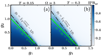
Figure 1: Inverse participation ratio of the ground state of the effective Hamiltonian in Eq. (5) as a function of the coupling parameters $g_{1}$ and $g_{2}$; $\Omega=3$ and $T$ is indicated. The green solid line represents the critical line for the QPT of the undriven case and the black dashed-dotted line is the modified critical line for the periodically driven system; $N=10$ and $n_{\text{max}}=199$.

The line determined by Eq. (6) is marked with a black dashed-dotted curve in Fig. 1. In comparison with the green line for the undriven system, one sees that with proper choices of the driving parameters $T$ and $\Omega$, the normal phase can be extended. Fig. 1 corresponds to the ground-state phase diagram for the effective Hamiltonian $H_{\text{eff}}$ in Eq. (5). The different shades of blue indicate the numerical value of the inverse participation ratio

$$\text{IPR}_{\text{gs}}=\sum_{n,m}|c_{n,m}|^{4},$$

of the ground state $|\psi_{\text{gs}}\rangle$, where $c_{n,m}=\langle{\cal B}_{n,m}|\psi_{\text{gs}}\rangle$. This quantity measures the level of delocalization of the ground state with respect to the basis states. When the ground state coincides with a basis state, $\text{IPR}_{\text{gs}}=1$, while a very delocalized ground state has $\text{IPR}_{\text{gs}}\propto{\cal N}^{-1}$. In Fig. 1, darker tones of blue indicate more localization. The values of $\text{IPR}_{\text{gs}}$ are shown as a function of the coupling parameters $g_{1}$ and $g_{2}$ for two values of the driving period, namely $T=0.15$ [Fig. 1(a)] and $T=0.2$ [Fig. 1(b)]. The abrupt separation between dark blue (normal phase) and light blue (superradiant phase) coincides with the critical line (black dashed-dotted line) obtained in Eq. (6). The panels make it clear that as the period increases ($\omega_{\text{d}}$ decreases), the critical line appears at larger values of the coupling parameters, which indicates that the normal phase gets extended.

III.2 Level Statistics

As mentioned above, the anisotropic Dicke model presents regular and chaotic regimes that can be identified in the quantum domain with the analysis of level statistics. Here, we investigate how the two regimes get affected by the presence of the periodic drive. For this, we consider the ratio of consecutive levels, defined as [16, 78]

$$r_{\nu}=\frac{\text{min}(s_{\nu-1},s_{\nu})}{\text{max}(s_{\nu-1},s_{\nu})},$$

where $s_{\nu}=\epsilon_{\nu+1}-\epsilon_{\nu}$ is the spacing between consecutive quasienergies (or between consecutive eigenvalues in the case of time-independent Hamiltonians). In the regular regime, where the nearest neighboring level spacing distribution is Poissonian, the average level spacing ratio $\langle r\rangle\approx 0.386$. For chaotic systems described by time-dependent Hamiltonians, level statistics depends on the driving frequency. If the frequency is high and ${\cal H}(t)$ is well described by a chaotic static effective Hamiltonian that is real and symmetric, thus exhibiting time-reversal symmetry, the level spacing distribution follows the Gaussian orthogonal ensemble (GOE) and $\langle r\rangle\approx 0.536$. On the other hand, if the frequency is small and $U(T)$ is a symmetric unitary matrix, level statistics follows that of a circular orthogonal ensemble (COE) and $\langle r\rangle\approx 0.527$ [16]. In finite systems, the repulsion is slightly stronger for GOE than for COE, but the results for both ensembles should coincide in the thermodynamic limit [16].

For the undriven anisotropic Dicke model, chaos emerges for large values of the coupling parameters $g_{1}$ and $g_{2}$, as shown in the inset of Fig. 2(d). Lower and upper band energies, which are in the nonchaotic region, are discarded for the analysis of level statistics. We use this figure as a reference for our choices of $g_{1}$ and $g_{2}$ in the driven scenario. The main panels in Fig. 2 display the average level spacing ratio for the driven system using different values of the bosonic cutoff $n_{\text{max}}$. The results are shown as a function of the driving frequency in Figs. 2(a,c) and as a function of the driving frequency rescaled by the energy bandwidth $\Delta$ of the undriven system in Figs. 2(b,d). The purpose of the rescaling is to check the convergence of the results. The solid lines for the different values of $n_{\text{max}}$ in Figs. 2(b,d) are indeed close and, for large frequencies, they nearly coincide with the curve for the effective Hamiltonian from Eq. (5) (dashed line), the agreement being excellent for the largest value of $n_{\text{max}}=199$. Notice that our $H_{\text{eff}}$ depends on the value of $T$, which contrasts with similar plots from previous studies, where the effective Hamiltonian used was obtained to zeroth-order of the Magnus expansion [16].

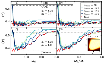
Figure 2: Average consecutive level spacing ratio, $\langle r\rangle$, of the anisotropic Dicke model as a function of the driving frequency (a,c) and of the driving frequency rescaled by the energy bandwith of the undriven system (b,d) for $g_{2}=0.1$ (a)-(b) and $g_{2}=1.0$ (c)-(d). We fix $g_{1}=1.25$, $\Omega=1$, and atom number $N=10$. Different bosonic cut-offs are used as indicated in the legend. The inset of panel (d) gives $\langle r\rangle$ as a function of $g_{1}$ and $g_{2}$ for the undriven model.

For the chosen coupling parameters in Figs. 2(a,b), the undriven system is regular, while in Figs. 2(c,d) it is chaotic. This explains why, at high frequencies, $\langle r\rangle$ in Figs. 2(a,b) reaches Poisson values, while $\langle r\rangle$ in Figs. 2(c,d) reaches GOE values. The saturation at the GOE value for large $\omega_{\text{d}}$ is more evident for the largest $n_{\text{max}}$. At low frequencies, the effective Hamiltonian ceases to be valid and the system becomes chaotic, independently of the regime of the undriven case. In this case, $\langle r\rangle$ should approach the COE value.

This last paragraph is dedicated to a possible explanation of what happens at the intermediate frequencies in Figs. 2(c,d), where one sees a significant dip in the values of $\langle r\rangle$. This may not be caused by a transition to a regular regime and may instead be an artifact of the process of folding the quasienergies to the principal Floquet zone $\left[-\omega_{\text{d}}/2,\omega_{\text{d}}/2\right]$. We discuss why we suspect this might be the case, but a final answer requires the analysis of the system in the classical limit [79]. As noticed in [16] and clearly explained in [80], at intermediate frequencies, some of the quasienergies lie outside the principal Floquet zone and need to be folded back. In this process, the folded quasienergies may not repel the energies originally inside the zone, resulting in a reduced value of $\langle r\rangle$. This contrasts with the case of a driving frequency larger than the many-body bandwidth $(\omega_{\text{d}}\gg\Delta)$, where the reconstruction of the spectrum of quasienergies is not required and the picture is analogous to that of a time-independent GOE Hamiltonian. It also contrasts with the case of low frequency, where the majority of the quasienergies need to be folded back and one reaches the scenario of COE statistics. It calls attention, however, that instead of a small dip suggesting a mixed scenario with some levels still repelling each other, as seen in [16, 80], our results for $\langle r\rangle$ reach Poisson values and the dip does not diminish as $n_{\text{max}}$ increases. We blame this result to the strong asymmetric shape of the density of states. It may be that at intermediate frequencies, the folded levels affect the states at high excitation energies, for which the GOE statistics used to hold, while the states at lower energies, which are not chaotic, do not get affected. Our speculation finds support in the quantum dynamics described in the next subsection, where despite the Poisson values associated with $\langle r\rangle$, the quantum evolution suggests spreading of the initial state at least comparable to what happens to the chaotic undriven Hamiltonian. However, we call attention to the puzzling results in Fig. 3(b) and Fig. 7.

III.3 Dynamics and Dependence on the Initial State

To study the dynamics, we consider the average boson number, defined as

$$N_{\text{av}}(t)=\langle\Psi(t)|a^{\dagger}a|\Psi(t)\rangle,$$ (7)

where $|\Psi(0)\rangle$ is the initial state, and the von Neumann entanglement entropy between the spins and bosons:

$$S(t)=-\text{Tr}\left[\rho_{\text{spins}}(t)\ln(\rho_{\text{spins}}(t))\right],$$ (8)

where $\rho_{\text{spins}}(t)=\text{Tr}_{\text{bosons}}\left[\rho(t)\right]$ is the reduced density matrix of the spins obtained by tracing over the bosonic degrees of freedom.

One expects generic driven systems to heat up and reach an infinite-temperature-like state with $\rho^{\infty}=\mathcal{I}/\mathcal{N}$ where $\mathcal{I}$ is the identity matrix and $\mathcal{N}$ is the Hilbert-space dimension. The infinite-temperature value of the average boson number for the Dicke model corresponds to

$$N_{\text{av}}^{\infty}=\text{Tr}\left[\rho^{\infty}_{\text{bosons}}a^{\dagger}a\right]=n_{\text{max}}/2,$$

where $\rho_{\text{bosons}}^{\infty}=\text{Tr}_{\text{spins}}\left[\rho^{\infty}\right]$, and the entanglement entropy saturates to the Page value [81], given by

$$S_{\text{Page}}=\text{ln}(N+1)-\frac{N+1}{2(n_{\text{max}}+1)}.$$

The Page value is derived for bounded systems, while the Hilbert space of the bosonic subspace of the Dicke model is unbounded. Yet, the truncation to $n_{\text{max}}$ still provides a meaningful result for the converged states. In what follows, we fix the atom number to $N=10$ and the bosonic mode cut-off at $n_{\text{max}}=199$, which gives $N_{\text{av}}^{\infty}\approx 100$ and $S_{\text{page}}\approx 2.37$. Our initial states are eigenstates of the decoupled Hamiltonian ($\tilde{g}(t)=0$). We average the data over 50 initial states.

In Fig. 3, we select coupling parameters corresponding to the chaotic undriven model and analyze the evolution of $N_{\text{av}}(t)$ [Figs. 3(a)-(b)] and $S(t)$ [Figs. 3(c)-(d)] for initial states with low [Figs. 3(a,c)] and high [Figs. 3(b,d)] energies, and under various choices of the driving frequency. The results are compared with the dynamics for the time-independent effective Hamiltonian in Eq. (5) (indicated as $\omega_{\text{d}}=\infty$ in the figure) and with the result for the infinite-temperature state (black dashed line).

In Figs. 3(a,c), where the initial states have low energy, as the driving frequency decreases and level statistics moves from GOE to COE, the saturation values for $N_{\text{av}}(t)$ and $S(t)$ increase monotonically, going from agreement with the result for the chaotic effective Hamiltonian to agreement with the infinite-temperature state. Nothing in the figure suggests any special feature for intermediate frequencies that would justify associating the dip for $\langle r\rangle$ seen in Fig. 2 with an enhancement of regular behavior. Below, after some additional discussions about the low-energy initial states, we investigate what happens when the initial states have high energies. In this case, a non-monotonic behavior with $\omega_{\text{d}}$ emerges, but only for the saturation values for $N_{\text{av}}(t)$ and in a very narrow range of intermediate values of the driving frequency.

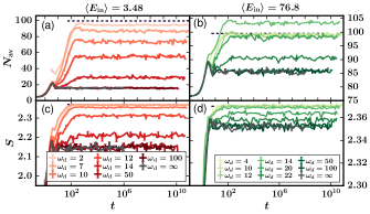
Figure 3: (a,b) Average boson number, $N_{\text{av}}(t)$, and (c,d) von-Neumann entanglement entropy $S(t)$ as a function of the stroboscopic time $t_{n}=nT$ for the periodically driven anisotropic Dicke model. Panels (a,c): low energy initial states, so that $\langle E_{\text{in}}\rangle=3.48$. Panels (b,d): high energy initial states, so that $\langle E_{\text{in}}\rangle=76.8$. The parameters $g_{1}=1.25,\ g_{2}=1.0$ guarantee chaos in the absence of a drive. The driving frequencies are indicated; the gray line represents the evolution under the effective time-independent Hamiltonian in Eq. (5); the black dashed indicates the results for the infinite-temperature state. For all plots the driving amplitude $\Omega=1.0$, $N=10$, $n_{\text{max}}=199$.

For high and intermediate driving frequencies, where $H_{\text{eff}}$ approximately describes the system, the saturation values for $N_{\text{av}}(t)$ and $S(t)$ found in Figs. 3(a,c) decrease if we decrease the value of $g_{2}$ (see Fig. 6 in appendix B). This is expected, because decreasing $g_{2}$ brings the effective Hamiltonian closer to the regular regime. The limited spread in the Hilbert space of the low energy states seen in Figs. 3(a,c), despite the drive and the chaoticity of $H_{\text{eff}}$, evokes the discussions in Ref. [82], where long-lived prethermal plateaus were observed for driven many-body spin chains under periodic drives at intermediate frequencies. It is possible that the spectrum of our model at low energies presents some special feature, such as a commensurate structure, that the periodic drive with intermediate frequencies cannot overcome. This is a point that deserves further investigation.

Under the periodic drive, one can increase the saturation values of the average boson number and the entanglement entropy by increasing the energies of the initial states, as seen in Figs. 3(b,d). Notice that the scale in the $y$-axis of these panels is not the same as in Figs. 3(a,c). For high-energy initial states, as seen in Fig. 3(d), the saturation values of $S(t)$ become close to the infinite-temperature state not only for low frequencies, but also for a range of intermediate frequencies. The results for the average boson number are, however, intriguing. Contrary to what we see for the entropy, the saturation value of $N_{\text{av}}(t)$ does not increase monotonically to the infinite-temperature result as we decrease $\omega_{\text{d}}$. Instead, for $\omega_{\text{d}}\lesssim 20$, we observe that $N_{\text{av}}^{\text{sat}}>N_{\text{av}}^{\infty}$ (see results for $N_{\text{av}}^{\text{sat}}$ vs $\omega_{\text{d}}$ and for $S^{\text{sat}}$ vs $\omega_{\text{d}}$ for different values of the initial state energy in Fig. 7 of the appendix B). The overshooting suggests lack of equipartition and predominant contributions from states with large average boson number. This means that for all driving frequencies $\omega_{\text{d}}\gtrsim 5$, even when $N_{\text{av}}^{\text{sat}}$ crosses $N_{\text{av}}^{\infty}$, there is no ergodicity, as supported by the saturating values of the entropy, which for this range of driving frequencies give $S^{\text{sat}}<S^{\infty}$.

The results in Fig. 3 and Fig. 6 are in stark contrast to what we observe for the quasiperiodic drive, where after a transient time, heating does take place. As we show in the next section, even for intermediate to high frequencies and small $g_{2}$, the quasiperiodic drive is capable of bringing the system to the infinite-temperature state after prethermalization. In Fig. 3, no matter how far in time we went, we never saw $N_{\text{av}}(t)$ and $S(t)$ getting away from their plateaus towards the infinite-temperature results. The periodically driven Dicke model with intermediate to high frequencies is thus well protected against heating, specially when it is prepared in a low-energy state.

IV Quasiperiodic drive

We now consider the case where the time-dependent drive is quasiperiodic, consisting either of Thue-Morse or Fibonacci sequences. The Thue-Morse sequence [65, 66, 67, 68, 69, 70] is constructed with unitary operators $U_{\pm}=\exp(-iH_{\pm}T)$, so that it starts with $U_{1}=U_{-}U_{+}$ and is followed by $\tilde{U}_{1}=U_{+}U_{-}$. Next, $U_{2}=\tilde{U}_{1}U_{1}$ is followed by $\tilde{U}_{2}=U_{1}\tilde{U}_{1}$, and so on successively. One can recursively construct the driving unit cells of time length $2^{n}T$ as $U_{n+1}=\tilde{U}_{n}U_{n}$. The Fibonacci sequence [71, 72, 73] is constructed using the recursive relation $U_{n}=U_{n-2}U_{n-1}$ for $n\geq 2$, where the initial unitary operators are $U_{0}=\text{exp}(-iH_{+}T)$ and $U_{1}=\text{exp}(-iH_{-}T)$. We discuss the case of the Thue-Morse drive in this section and present the analysis of the Fibonacci drive in appendix C. The results for both cases are similar, but the dependence of the heating time on the driving frequency is different.

In Fig. 4, we consider low-energy initial states and the Thue-Morse driving sequence. We show the dynamics of the average boson number [Fig. 4(a)-(b)] and the entanglement entropy [Fig. 4(c)-(d)] for a fixed intermediate value of the driving frequency $\omega_{\text{d}}$ and various values of the coupling parameter $g_{2}$ [Fig. 4(a,c)] and for a fixed $g_{2}$ associated with the chaotic undriven model and various values of $\omega_{\text{d}}$ [Fig. 4(b,d)]. All panels exhibit a prethermal plateau followed by a saturation to the infinite-temperature state, which contrasts with the results in Fig. 3 (a,c). The quasiperiodic drive breaks regularity and induces ergodicity. It causes all cases considered with intermediate frequency and coupling parameters from the regular to the chaotic regime to heat up to an infinite temperature.

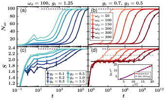
Figure 4: (a)-(b) Average boson number, $N_{\text{av}}(t)$, and (c)-(d) von-Neumann entanglement entropy, $S(t)$, as a function of time $t_{n}=2^{n}T$ for the anisotropic Dicke model under the Thue-Morse quasiperiodic drive. The initial states have low energies, so that $\langle E_{\text{in}}\rangle=3.48$. Panels (a,c): intermediate driving frequency $\omega_{\text{d}}=100$, $g_{1}=1.25$, and various values of $g_{2}$. Panels (b,d): $g_{1}=0.7$, $g_{2}=0.5$ for a chaotic undriven system and various values $\omega_{d}$ . The inset in Fig. 4(d) shows the scaling of the heating time $\tau^{*}$ with $\omega_{\text{d}}$; numerical data are in blue and the best fitting, given by $\log\tau^{*}=1.4\sqrt{\omega_{\text{d}}}-4.24$, is in red. In all panels, the driving amplitude is $\Omega=1.0$, $N=10$, and $n_{\text{max}}=199$. The dashed line represents the Page value, the black solid line is for the prethermal value, and the dashed-dotted line represents the value when the entanglement entropy reaches the halfway mark between its prethermal plateau and the Page value.

The prethermal plateau gets longer in time if one increases the driving frequency or brings the coupling parameters closer to the regular regime. To quantify the dependence of the prethermal plateau on the driving frequency, we study the heating time $\tau^{*}$, which is defined as the time when the entanglement entropy reaches the halfway mark between its prethermal plateau and the Page value [21], $S(\tau^{*})\equiv S_{p}+[S_{\text{page}}-S_{p}]/2$. The inset in Fig. 4(d) shows that for the Thue-Morse drive protocol, the heating time $\tau^{*}$ grows as a stretched exponential with $\omega_{\text{d}}$, the best fitting curve corresponding to $\log\tau^{*}=1.55\sqrt{\omega_{\text{d}}}-0.695$. In appendix C, we show that for the Fibonacci drive protocol, the heating time grows exponentially with the driving frequency as $\log\tau^{*}=0.125\omega_{\text{d}}-0.39$.

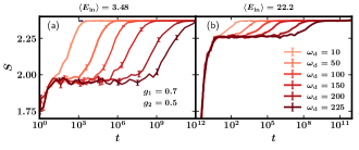
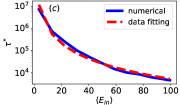
Figure 5: Entanglement entropy as a function of the sequential time $t_{n}=2^{n}T$ for the anisotropic Dicke model under the Thue-Morse quasiperiodic drive; $g_{1}=0.7,\ g_{2}=0.5$. Results averaged over $50$ initial states with (a) low energy, $\langle E_{\text{in}}\rangle=3.48$, and (b) high energy, $\langle E_{\text{in}}\rangle=22.2$. Panel (c): heating time as a function of $\langle E_{\text{in}}\rangle$ for a fixed driving frequency, $\omega_{\text{d}}=200$; the time scales as $\tau^{*}=[1.99\times 10^{8}]{E_{\text{in}}}^{-2.29}$. The driving amplitude is $\Omega=1.0$, $N=10$, and $n_{\text{max}}=199$.

In Fig. 5, we extend the analysis done in Fig. 4 and investigate how our results are affected by the rise of the energies of the initial states. In Figs. 5 (a)-(b), we plot the evolution of the entanglement entropy for two sets of initial states with different energies, respectively given by $\langle E_{\text{in}}\rangle=3.48$ and $\langle E_{\text{in}}\rangle=22.2$. As the energy increases, the prethermal plateau happens at higher values and the heating time decreases. To check the energy dependence on the heating time, we plot $\tau^{*}$ as a function of $\langle E_{\text{in}}\rangle$ in Fig. 5 (c). We verify that for the Thue-Morse drive protocol, $\tau^{*}$ decays as $E_{\text{in}}^{-2.29}$. In appendix C, we show that for the Fibonacci drive protocol, $\tau^{*}$ decays as $E_{\text{in}}^{-4.03}$.

V Summary

We studied the effects that a periodic drive and a quasiperiodic drive have on the anisotropic Dicke model. While we have verified that some of the results are similar to those for the driven isotropic Dicke model (not shown), this work focusses on the more general anisotropic Dicke model. We list below our four main findings.

(i) Using a periodic drive and the high-frequency Magnus expansion, we provided a modified condition for the normal to superradiant QPT. By properly choosing the driving frequency, one can extend the normal phase.

(ii) We argued that the results for level statistics suggesting regularity for the periodically driven system under intermediate frequencies may be an artifact caused by the folding procedure of the quasienergies back to the principal Floquet zone and the highly asymmetric shape of the density of states.

(iii) Under the periodic drive, the system saturates to a steady state value that is not followed by heating to the infinite-temperature state. The saturation values depend on the energy of the initial state, the frequency of the drive, and the parameters of the undriven Hamiltonian. To reach saturation values that indicate near ergodicity, small driving frequencies are required. Therefore, the non-monotonic behavior of the saturation values of the average boson number observed for intermediate driving frequencies imply that these frequencies are still not small enough to ensure equipartition.

(iv) For the quasiperiodic drives, prethermalization is followed by heating, ensuring full ergodicity. The heating time $\tau^{*}$ for the Fibonacci protocol grows exponentially with the driving frequency ($\tau^{*}\propto e^{\omega_{\text{d}}})$, while for the Thue-Morse protocol the growth follows a stretched exponential ($\tau^{*}\propto e^{\sqrt{\omega_{\text{d}}}})$. In both cases, the heating time decreases as the energy of the initial state increases.

Overall, our work shows that the (anisotropic) Dicke model exhibits properties of genuinely many-body quantum systems that could be experimentally explored. The absence of heating for the periodic drive and the long prethermal plateaus for the quasiperiodic drives, for example, provide scenarios under which non-equilibrium phases of matter could be hosted.

There are different future directions that we plan to investigate. Among them, our priorities are the role of dissipation and a comparison between the quantum and classical dynamics.

Appendix A Periodic drive

In this appendix, we derive in Sec. A.1 the analytical expression of the effective Hamiltonian for the periodically driven anisotropic Dicke model using the high-frequency Floquet-Magnus expansion. In Sec. A.2, we derive the modified equation for the critical line of the QPT due to the periodic drive.

A.1 Derivation of the effective Hamiltonian

We first recall the system Hamiltonian in Eq. (1):

$${\cal H}(t) = \omega a^{\dagger}a+\omega_{0}J_{z}+\frac{\tilde{g}_{1}(t)}{\sqrt{2j}}(a^{\dagger}J_{-}+aJ_{+})+$$ (9)

$$\frac{\tilde{g}_{2}(t)}{\sqrt{2j}}(a^{\dagger}J_{+}+aJ_{-}).$$

The protocol of the square wave periodic drive applied to the system is

$$\tilde{g}_{i}(t) = g_{i}+\Omega\hskip 25.60747pt0<t\leq\frac{T}{2},$$

$$\tilde{g}_{i}(t) = g_{i}-\Omega\hskip 25.60747pt\frac{T}{2}<t\leq T.$$

This means that the system is periodically driven by a repeated two-step sequence that alternates between the time-independent Hamiltonians $H+V$ and $H-V$ (see main text). The duration of each step is $T/2$, where $T=2\pi/\omega_{\text{d}}$ is the period of the driving sequence. The evolution operator at time $t=nT$ is

$$U(t=nT)=\left(e^{-iT(H-V)/2}e^{-iT(H+V)/2}\right)^{n}.$$ (10)

Using the Magnus expansion and small $T$, we search for a time-independent effective Hamiltonian $H_{\text{eff}}$ that approximately describes the evolution as

$$U(t=nT)\approx e^{-inTH_{\text{eff}}}.$$ (11)

Since the driving protocol involves time-independent Hamiltonians, the Magnus expansion coincides with the Baker-Campbell-Hausdorff expansion, where the product of two exponentials can be simplified to

$$e^{X}e^{Y}=e^{\left(X+Y+\frac{1}{2}[X,Y]+\frac{1}{12}[X-Y,[X,Y]]+...\right)}.$$ (12)

Let

$$X=\frac{1}{2}(H-V),\hskip 14.22636ptY=\frac{1}{2}(H+V),$$ (13)

then

$$X+Y=H,\hskip 14.22636ptX-Y=-V,$$ (14)

$$[X,Y]=\frac{1}{4}[H-V,H+V]=\frac{1}{2}[H,V],$$ (15)

and

$$H_{\text{eff}} = H+\frac{T}{2i}[X,Y]-\frac{T^{2}}{12}[[X,Y],V]+...$$ (16)

After some calculation, we have

$$[X,Y]=\frac{\omega\Omega}{\sqrt{N}}(a^{\dagger}-a)J_{x}+\frac{\omega_{0}\Omega}{\sqrt{N}}(a^{\dagger}+a)iJ_{y}$$

$$+\frac{(g_{1}-g_{2})\Omega}{\sqrt{N}}(2iJ_{x}J_{y}-(a^{\dagger}-a)(a^{\dagger}+a)J_{z}),$$ (17)

and

$$[X-Y,[X,Y]] = [[X,Y],V]=$$

$$-\frac{4\omega\Omega^{2}}{N}J_{x}^{2}+\frac{2\omega_{0}\Omega^{2}}{N}(a^{\dagger}+a)(a^{\dagger}+a)J_{z}$$

$$+\frac{(g_{1}-g_{2})\Omega^{2}}{N\sqrt{N}}\Big{(}8(a^{\dagger}+a)J_{x}J_{z}+$$

$$(a^{\dagger}-a)({a^{\dagger}+a}^{2})(J_{+}-J_{-})\Big{)}.$$

The first order term, $\frac{T}{2i}[X,Y]=-i\frac{T}{4}[H,V]$, is imaginary which breaks the time reversal symmetry [83]. Hence we discard the first order term and consider the second order correction shown above, which leads to

$$H_{\text{eff}} = \omega a^{\dagger}a+\omega_{0}J_{z}+\frac{g_{1}}{\sqrt{N}}(a^{\dagger}J_{-}+aJ_{+})+\frac{g_{2}}{\sqrt{N}}(a^{\dagger}J_{+}$$ (19)

$$+aJ_{-})-\frac{T^{2}}{12}\Big{[}-\frac{4\omega\Omega^{2}}{N}J_{x}^{2}+\frac{2\omega_{0}\Omega^{2}}{N}(a^{\dagger}+a)\times$$

$$(a^{\dagger}+a)J_{z}+\frac{(g_{1}-g_{2})\Omega^{2}}{N\sqrt{N}}\Big{(}8(a^{\dagger}+a)J_{x}J_{z}+$$

$$(a^{\dagger}-a)({a^{\dagger}+a})^{2}(J_{+}-J_{-})\Big{)}\Big{]}.$$

A.2 Critical line of the quantum phase transition of the driven system

To find the critical line, we first apply the Holstein-Primakoff transformation [33] to the effective Hamiltonian in Eq. (19),

$$J_{+}=b^{\dagger}\sqrt{2j-b^{\dagger}b},\hskip 8.53581ptJ_{-}=\sqrt{2j-b^{\dagger}b}\hskip 2.84526ptb,\hskip 8.53581ptJ_{z}=b^{\dagger}b-j.$$ (20)

In the thermodynamic limit (when the atom number $N\to\infty$), we have

$$H_{\text{eff}} = \omega a^{\dagger}a+\omega_{0}b^{\dagger}b+g_{1}(a^{\dagger}b+ab^{\dagger})+g_{2}(a^{\dagger}b^{\dagger}+ab)$$ (21)

$$+\frac{T^{2}\omega\Omega^{2}}{12}\left({b^{\dagger}}^{2}+b^{2}\right)+\frac{T^{2}\omega\Omega^{2}}{6}b^{\dagger}b$$

$$+\frac{T^{2}\omega_{0}\Omega^{2}}{6N}\frac{N}{2}\left({a^{\dagger}}^{2}+a^{2}+2a^{\dagger}a+1\right)$$

$$-\frac{T^{2}\omega_{0}\Omega^{2}}{6N}\left({a^{\dagger}}^{2}+a^{2}\right)(b^{\dagger}b)-\frac{T^{2}\omega_{0}A^{2}}{6N}2(a^{\dagger}a)(b^{\dagger}b)$$

$$-\frac{T^{2}\omega_{0}\Omega^{2}}{6N}b^{\dagger}b+\frac{T^{2}\Delta g\Omega^{2}}{3N}\frac{N}{2}(a+a^{\dagger})(b+b^{\dagger})$$

$$-\frac{T^{2}\Delta g\Omega^{2}}{3N}(a+a^{\dagger})(b+b^{\dagger})b^{\dagger}b$$

We now consider only up to second order terms in the bosonic operators, which means that we neglect the last term of the Hamiltonian in Eq. (19). Introducing the position and momentum operators for the two bosonic modes as

$$x=\frac{1}{\sqrt{2\omega}}(a^{\dagger}+a),\hskip 8.53581ptp_{x}=i\sqrt{\frac{\omega}{2}}(a^{\dagger}-a),$$

$$y=\frac{1}{\sqrt{2\omega_{0}}}(b^{\dagger}+b),\hskip 8.53581ptp_{y}=i\sqrt{\frac{\omega_{0}}{2}}(b^{\dagger}-b),$$ (22)

we have:

$$H_{\text{eff}} = \left(1+\frac{T^{2}\Omega^{2}\omega_{0}}{6\omega}\right)\frac{1}{2}(\omega^{2}x^{2}+p_{x}^{2}-\omega)$$ (23)

$$+\left(1+\frac{T^{2}\Omega^{2}\omega}{6\omega_{0}}+\frac{T^{2}\Omega^{2}}{6N}\right)\frac{1}{2}(\omega_{0}^{2}y^{2}+p_{y}^{2}-\omega_{0})$$

$$+g_{1}\left(\sqrt{\omega\omega_{0}}xy+\frac{p_{x}p_{y}}{\sqrt{\omega\omega_{0}}}\right)+g_{2}\Big{(}\sqrt{\omega\omega_{0}}xy$$

$$-\frac{p_{x}p_{y}}{\sqrt{\omega\omega_{0}}}\Big{)}+\frac{T^{2}\Omega^{2}\omega}{12}\left(\omega_{0}y^{2}-\frac{p_{y}^{2}}{\omega_{0}}\right)$$

$$+\frac{T^{2}\Omega^{2}\omega_{0}}{12}\left(\omega x^{2}-\frac{p_{x}^{2}}{\omega}\right)+\frac{T^{2}\Omega^{2}\omega_{0}}{12N}\left(\omega x^{2}-\frac{p_{x}^{2}}{\omega}\right)$$

$$+\frac{T^{2}\Omega^{2}\omega_{0}}{12N}\Big{(}\omega x^{2}+\frac{p_{x}^{2}}{\omega}+\omega_{0}y^{2}+\frac{p_{y}^{2}}{\omega_{0}}\Big{)}$$

$$+\frac{T^{2}\Omega^{2}\Delta g}{3}\sqrt{\omega\omega_{0}}xy+\frac{T^{2}\Omega^{2}\Delta g}{3N}\sqrt{\omega\omega_{0}}xy.$$

To find the critical line for the QPT, we just need to resort to the position part of the equation, which is given by

$$H_{\text{eff}}^{\tilde{x},\tilde{y}} = \frac{1}{2}\left(\tilde{x}^{2}+\tilde{y}^{2}+\frac{2\gamma}{\alpha\beta\sqrt{\omega\omega_{0}}}\tilde{x}\tilde{y}\right),$$ (24)

where, $\tilde{x}=\omega\alpha x$, $\tilde{y}=\omega_{0}\beta y$, and

$$\alpha^{2} = \left(1+\frac{T^{2}\Omega^{2}\omega_{0}}{3\omega}+\frac{T^{2}\Omega^{2}\omega_{0}}{3N\omega}\right),$$

$$\beta^{2} = \left(1+\frac{T^{2}\Omega^{2}\omega}{3\omega_{0}}\right),$$

$$\gamma = \left(g_{1}+g_{2}+\frac{T^{2}\Omega^{2}\Delta g}{3}+\frac{T^{2}\Omega^{2}\Delta g}{3N}\right).$$

Introducing normal coordinates,

$$q_{+}=\frac{(\tilde{x}+\tilde{y})}{\sqrt{2}},\hskip 8.53581ptq_{-}=\frac{(\tilde{x}-\tilde{y})}{\sqrt{2}},$$ (25)

we have

$$H_{\text{eff}}^{q_{+},q_{-}} = \frac{1}{2}\left[\left(q_{+}^{2}+q_{-}^{2}\right)+\frac{\gamma}{\alpha\beta\sqrt{\omega\omega_{0}}}\left(q_{+}^{2}-q_{-}^{2}\right)\right]$$

$$= \frac{1}{2}\left[\left(1+\frac{\gamma}{\alpha\beta\sqrt{\omega\omega_{0}}}\right)q_{+}^{2}+\left(1-\frac{\gamma}{\alpha\beta\sqrt{\omega\omega_{0}}}\right)q_{-}^{2}\right].$$

From the equation of motion for $q_{-}$, which is $\ddot{q}_{-}=-\left(1-\frac{\gamma}{\alpha\beta\sqrt{\omega\omega_{0}}}\right)q_{-}$, one gets the equation of the critical line for the QPT in the $g_{1}-g_{2}$ plane,

$$1-\frac{\gamma}{\alpha\beta\sqrt{\omega\omega_{0}}}=0.$$ (27)

Introducing the notation $\delta=\frac{T^{2}\Omega^{2}}{3}$, we have

$$g_{1}+g_{2} = \Big{(}1+\frac{\delta\omega}{2\omega_{0}}+\frac{\delta\omega_{0}}{2\omega}+\frac{\delta\omega_{0}}{2N\omega}\Big{)}\sqrt{\omega\omega_{0}}$$ (28)

$$-\delta\Delta g-\frac{\delta\Delta g}{N},$$

where $\Delta g=g_{1}-g_{2}$ and we have not considered the other higher order terms as $\delta<<1$. In the thermodynamic limit ($N\to\infty$), we finally obtain

$$g_{1}+g_{2} = \Big{(}1+\frac{\delta\omega}{2\omega_{0}}+\frac{\delta\omega_{0}}{2\omega}\Big{)}\sqrt{\omega\omega_{0}}-\delta\Delta g.$$ (29)

or,

$$(1+\delta)g_{1}+(1-\delta)g_{2} = \Big{(}1+\frac{\delta}{2}\Big{(}\frac{\omega}{\omega_{0}}+\frac{\omega_{0}}{\omega}\Big{)}\Big{)}\sqrt{\omega\omega_{0}}$$

and hence,

$$g_{2} = \left(\frac{1+\tilde{\delta}}{1-\delta}\right)\sqrt{\omega\omega_{0}}-\left(\frac{1+\delta}{1-\delta}\right)g_{1},$$ (31)

where $\tilde{\delta}=\frac{\delta}{2}\left(\frac{\omega}{\omega_{0}}+\frac{\omega_{0}}{\omega}\right)$. or,

$$g_{2} = \tilde{\chi}\sqrt{\omega\omega_{0}}-\chi g_{1},$$ (32)

where, $\chi=\left(\frac{1+\delta}{1-\delta}\right)$ and $\tilde{\chi}=\left(\frac{1+\tilde{\delta}}{1-\delta}\right)$.

Appendix B Periodic drive

This appendix extends the results presented in Fig. 3 of the main text.

B.1 Dependence on the coupling parameters

To complement Figs. 3(a,c) of the main text and support the discussion made there about the dependence of the saturation values of $N_{\text{av}}(t)$ and $S(t)$ on the coupling parameters, we show in Fig. 6 the evolution of the average boson number [Fig. 6(a)] and the entanglement entropy [Fig. 6(b)] for low-energy initial states and a fixed intermediate value of the driving frequency $\omega_{\text{d}}$. Various values of the coupling parameter $g_{2}$ are considered, so that the undriven Hamiltonian goes from the regular to the chaotic regime.

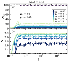
Figure 6: (a) Average boson number, $N_{\text{av}}(t)$, and (b) von-Neumann entanglement entropy $S(t)$ as a function of the stroboscopic time $t_{n}=nT$ for the periodically driven anisotropic Dicke model. The initial states have low energies, so that $\langle E_{\text{in}}\rangle=3.48$, as in Figs. 3(a,b). The driving frequency is fixed at an intermediate value, $\omega_{\text{d}}=50$ and various values of $g_{2}$ are considered, as indicated. The black dashed line indicates the results for the infinite-temperature state. For both panels, $g_{1}=1.25$, the driving amplitude is $\Omega=1.0$, $N=10$, and $n_{\text{max}}=199$.

As explained in the main text, for an intermediate frequency and low-energy initial states, the periodic drive is unable to bring $N_{\text{av}}(t)$ and $S(t)$ close to the results of the infinite-temperature state, at least not for the very long times that we studied. The saturation values of the two quantities are always below $N^{\infty}$ and $S_{\text{Page}}$ and, as shown in Fig. 6(a,c), they further decrease, as we decrease $g_{2}$ and the undriven model is brought closer to the regular regime.

B.2 Dependence on the initial state energy

Figure 7 shows the saturation values of average boson number (top panels: Fig. 7(a)-(c)) and of the von-Neumann entanglement entropy (bottom panels: Fig. 7(d)-(f)) as a function of the driving frequency for different values of the initial state energy. While $S^{\text{sat}}$ grows monotonically towards the infinite-temperature result as $\omega_{\text{d}}$ decreases, the same does not happen for $N_{\text{av}}^{\text{sat}}$ when the energy of the initial state is high. There is a very narrow range of driving frequencies where $N_{\text{av}}^{\text{sat}}>N_{\text{av}}^{\infty}$. This implies that the value of the driving frequency is still not small enough to ensure equipartition. As $\omega_{\text{d}}$ decreases from $\infty$, the fact that $N_{\text{av}}^{\text{sat}}$ crosses $N_{\text{av}}^{\infty}$, before becoming larger than it, is not caused by ergodicity, but by the significant number of states contributing to the dynamics, which have average boson number in the vicinity of $N_{\text{av}}^{\infty}$.

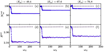
Figure 7: The saturation value of the average boson number (top panels) and of the von-Neumann entanglement entropy between spins and bosons (bottom panels) as a function of the driving frequency. The black dashed line indicates the infinite-temperature result. We fix $g_{1}=1.25,\ g_{2}=1.0$, $\Omega=1$, and atom number $N=10$, bosonic cut-off $n_{\text{max}}=199$.

Appendix C Fibonacci sequence

The results shown here for the Fibonacci quasiperiodic drive are similar to those shown in Sec. IV for the Thue-Morse quasiperiodic drive, with the difference that there $\tau^{*}\propto\exp(\sqrt{\omega_{\text{d}}})$, while here $\tau^{*}\propto\exp(\omega_{\text{d}})$. Figure 8 is equivalent to Fig. 4, and Fig. 9 is equivalent to Fig. 5.

In Fig. 8, we consider low-energy initial states and the Fibonacci driving sequence. We show the dynamics of the average boson number [Fig. 8(a)-(b)] and the entanglement entropy [Fig. 8(c)-(d)] for a fixed intermediate value of the driving frequency $\omega_{\text{d}}$ and various values of coupling parameter $g_{2}$ [Fig. 8(a,c)] and for a fixed $g_{2}$ associated with the chaotic undriven model and various values of $\omega_{\text{d}}$ [Fig. 8(b,d)]. All panels exhibit a prethermal plateau followed by the saturation to the infinite-temperature state. The prethermal plateau gets longer in time as we increase the driving frequency or bring the coupling parameters closer to the regular regime. The anisotropic Dicke model under this quasiperiodic drive heats up exponentially slowly, as shown in the inset of Fig. 4(d), where the heating time grows with $\omega_{\text{d}}$ as $\log\tau^{*}=0.125\omega_{\text{d}}-0.39$.

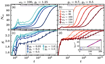
Figure 8: (a)-(b) Average boson number $N_{\text{av}}(t)$ and (c)-(d) von-Neumann entanglement entropy $S(t)$ as a function of time $t_{n}=t_{n-1}+t_{n-2}$ for the anisotropic Dicke model under the Fibonacci quasiperiodic drive. The initial states have low energies, so that $\langle E_{\text{in}}\rangle=3.48$. Panels (a,c): intermediate driving frequency $\omega_{\text{d}}=100$, $g_{1}=1.25$, and various values of $g_{2}$. Panels (b,d): $g_{1}=0.7$, $g_{2}=0.5$ for a chaotic undriven system and various values $\omega_{\text{d}}$ . The inset in panel (d) shows the scaling of the heating time $\tau^{*}$ with $\omega_{\text{d}}$; numerical data are in blue and the best fitting, given by $\log\tau^{*}=0.125\omega_{\text{d}}-0.39$, is in red. In all panels, the driving amplitude is $\Omega=1$, $N=10$, and $n_{\text{max}}=199$. In this figure the dashed line represent the page value, the black solid line is for the prethermal value whereas the dashed-dotted line represents the value when the entanglement entropy reaches the halfway mark between its prethermal plateau and the Page value.

In Fig. 9(a)-(b), we compare the evolution of the entanglement entropy for two different initial states energies, respectively $\langle E_{\text{in}}\rangle=3.48$ and $\langle E_{\text{in}}\rangle=22.2$. As the energy increases, the prethermal plateau happens at higher values and the heating time decreases. To check the energy dependence on the heating time, we plot $\tau^{*}$ as a function of $\langle E_{\text{in}}\rangle$ in Fig. 9 (c) and we verify that $\tau^{*}$ decays as $E_{\text{in}}^{-4.03}$.

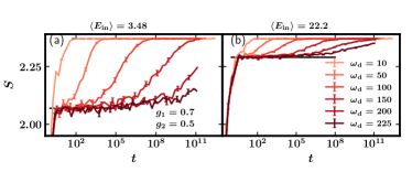
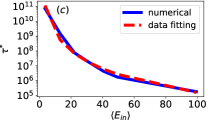
Figure 9: Entanglement entropy as a function of sequential time $t_{n}=t_{n-2}+t_{n-1}$ for the anisotropic Dicke model under the Fibonacci quasiperiodic drive; $g_{1}=0.7,\ g_{2}=0.5$. Results averaged over $50$ initial states with (a) low energy, $\langle E_{\text{in}}\rangle=3.48$ and (b) high energy, $\langle E_{\text{in}}\rangle=22.2$. Panel (c): heating energy as a function of $\langle E_{\text{in}}\rangle$ for a fixed driving frequency $\omega_{\text{d}}=200$ and it scales as: $\tau^{*}=[1.8034\times 10^{13}]{E_{\text{in}}}^{-4.03}$. The driving amplitude is $\Omega=1.0$, $N=10$ and $n_{\text{max}}=199$.

References

- Hahn [1950] E. L. Hahn, Spin echoes, Phys. Rev. 80, 580 (1950).
- Kapitza [1951] P. Kapitza, Dynamic stability of the pendulum with vibrating suspension point, Soviet Physics–JETP 21, 588 (1951).
- Casati et al. [1979] G. Casati, B. V. Chirikov, F. M. Izrailev, and J. Ford, Stochastic behavior of a quantum pendulum under a periodic perturbation, Lect. Notes in Phys. 9399, 334 (1979).
- Ueda [1979] Y. Ueda, Randomly transitional phenomena in the system governed by duffing’s equation, J. Stat. Phys. 20, 181 (1979).
- Marthaler and Dykman [2006] M. Marthaler and M. I. Dykman, Switching via quantum activation: A parametrically modulated oscillator, Phys. Rev. A 73, 042108 (2006).
- Zhang and Dykman [2017] Y. Zhang and M. I. Dykman, Preparing quasienergy states on demand: A parametric oscillator, Phys. Rev. A 95, 053841 (2017).
- Puri et al. [2017] S. Puri, S. Boutin, and A. Blais, Engineering the quantum states of light in a Kerr-nonlinear resonator by two-photon driving, NPJ Quantum Information 3, 18 (2017).
- Caprio et al. [2008] M. Caprio, P. Cejnar, and F. Iachello, Excited state quantum phase transitions in many-body systems, Annals of Physics 323, 1106 (2008).
- Cejnar et al. [2021] P. Cejnar, P. Stránský, M. Macek, and M. Kloc, Excited-state quantum phase transitions, J. Phys. A 54, 133001 (2021).
- Chinni et al. [2021] K. Chinni, P. M. Poggi, and I. H. Deutsch, Effect of chaos on the simulation of quantum critical phenomena in analog quantum simulators, Phys. Rev. Res. 3, 033145 (2021).
- Sáiz et al. [2023] A. Sáiz, J. Khalouf-Rivera, J. M. Arias, P. Pérez-Fernández, and J. Casado-Pascual, Quantum phase transitions in periodically quenched systems (2023), arXiv:2302.00382 [quant-ph] .
- Zhang et al. [2017] J. Zhang, P. W. Hess, A. Kyprianidis, P. Becker, A. Lee, J. Smith, G. Pagano, I.-D. Potirniche, A. C. Potter, A. Vishwanath, N. Y. Yao, and C. Monroe, Observation of a discrete time crystal, Nature 543, 217 (2017).
- Peng et al. [2021] P. Peng, C. Yin, X. Huang, C. Ramanathan, and P. Cappellaro, Floquet prethermalization in dipolar spin chains, Nature Physics 17, 444 (2021).
- Rubio-Abadal et al. [2020] A. Rubio-Abadal, M. Ippoliti, S. Hollerith, D. Wei, J. Rui, S. L. Sondhi, V. Khemani, C. Gross, and I. Bloch, Floquet prethermalization in a Bose-Hubbard system, Phys. Rev. X 10, 021044 (2020).
- Pyrialakos et al. [2022] G. G. Pyrialakos, J. Beck, M. Heinrich, L. J. Maczewsky, N. V. Kantartzis, M. Khajavikhan, A. Szameit, and D. N. Christodoulides, Bimorphic Floquet topological insulators, Nature Materials 21, 634 (2022).
- D’Alessio and Rigol [2014] L. D’Alessio and M. Rigol, Long-time behavior of isolated periodically driven interacting lattice systems, Phys. Rev. X 4, 041048 (2014).
- Lazarides et al. [2014] A. Lazarides, A. Das, and R. Moessner, Equilibrium states of generic quantum systems subject to periodic driving, Phys. Rev. E 90, 012110 (2014).
- Lazarides et al. [2015] A. Lazarides, A. Das, and R. Moessner, Fate of many-body localization under periodic driving, Phys. Rev. Lett. 115, 030402 (2015).
- Ponte et al. [2015] P. Ponte, A. Chandran, Z. Papić, and D. A. Abanin, Periodically driven ergodic and many-body localized quantum systems, Ann. Phys. (NY) 353, 196 (2015).
- Mori et al. [2016] T. Mori, T. Kuwahara, and K. Saito, Rigorous bound on energy absorption and generic relaxation in periodically driven quantum systems, Phys. Rev. Lett. 116, 120401 (2016).
- Bhakuni et al. [2021] D. S. Bhakuni, L. F. Santos, and Y. B. Lev, Suppression of heating by long-range interactions in periodically driven spin chains, Phys. Rev. B 104, L140301 (2021).
- Dicke [1954] R. H. Dicke, Coherence in spontaneous radiation processes, Physical review 93, 99 (1954).
- Hepp and Lieb [1973] K. Hepp and E. H. Lieb, On the superradiant phase transition for molecules in a quantized radiation field: the Dicke maser model, Annals of Physics 76, 360 (1973).
- Wang and Hioe [1973] Y. K. Wang and F. T. Hioe, Phase transition in the Dicke model of superradiance, Phys. Rev. A 7, 831 (1973).
- Baumann et al. [2010] K. Baumann, C. Guerlin, F. Brennecke, and T. Esslinger, Dicke quantum phase transition with a superfluid gas in an optical cavity, nature 464, 1301 (2010).
- Baumann et al. [2011] K. Baumann, R. Mottl, F. Brennecke, and T. Esslinger, Exploring symmetry breaking at the Dicke quantum phase transition, Phys. Rev. Lett. 107, 140402 (2011).
- Arnold et al. [2011] K. J. Arnold, M. P. Baden, and M. D. Barrett, Collective cavity quantum electrodynamics with multiple atomic levels, Phys. Rev. A 84, 033843 (2011).
- Baden et al. [2014] M. P. Baden, K. J. Arnold, A. L. Grimsmo, S. Parkins, and M. D. Barrett, Realization of the Dicke model using cavity-assisted raman transitions, Phys. Rev. Lett. 113, 020408 (2014).
- Klinder et al. [2015] J. Klinder, H. Keßler, M. R. Bakhtiari, M. Thorwart, and A. Hemmerich, Observation of a superradiant Mott insulator in the Dicke-Hubbard model, Phys. Rev. Lett. 115, 230403 (2015).
- Zhang et al. [2018] Z. Zhang, C. H. Lee, R. Kumar, K. J. Arnold, S. J. Masson, A. L. Grimsmo, A. S. Parkins, and M. D. Barrett, Dicke-model simulation via cavity-assisted raman transitions, Phys. Rev. A 97, 043858 (2018).
- Safavi-Naini et al. [2018] A. Safavi-Naini, R. J. Lewis-Swan, J. G. Bohnet, M. Gärttner, K. A. Gilmore, J. E. Jordan, J. Cohn, J. K. Freericks, A. M. Rey, and J. J. Bollinger, Verification of a many-ion simulator of the Dicke model through slow quenches across a phase transition, Phys. Rev. Lett. 121, 040503 (2018).
- Jaako et al. [2016] T. Jaako, Z.-L. Xiang, J. J. Garcia-Ripoll, and P. Rabl, Ultrastrong-coupling phenomena beyond the Dicke model, Phys. Rev. A 94, 033850 (2016).
- Emary and Brandes [2003a] C. Emary and T. Brandes, Chaos and the quantum phase transition in the Dicke model, Phys. Rev. E 67, 066203 (2003a).
- Chávez-Carlos et al. [2016] J. Chávez-Carlos, M. A. Bastarrachea-Magnani, S. Lerma-Hernández, and J. G. Hirsch, Classical chaos in atom-field systems, Phys. Rev. E 94, 022209 (2016).
- Buijsman et al. [2017] W. Buijsman, V. Gritsev, and R. Sprik, Nonergodicity in the anisotropic Dicke model, Phys. Rev. Lett. 118, 080601 (2017).
- Emary and Brandes [2003b] C. Emary and T. Brandes, Quantum chaos triggered by precursors of a quantum phase transition: The Dicke model, Phys. Rev. Lett. 90, 044101 (2003b).
- Lambert et al. [2004] N. Lambert, C. Emary, and T. Brandes, Entanglement and the phase transition in single-mode superradiance, Phys. Rev. Lett. 92, 073602 (2004).
- Zhu et al. [2019] G.-L. Zhu, X.-Y. Lü, S.-W. Bin, C. You, and Y. Wu, Entanglement and excited-state quantum phase transition in an extended Dicke model, Frontiers of Physics 14, 1 (2019).
- Hu and Wan [2021] J. Hu and S. Wan, Out-of-time-ordered correlation in anisotropic Dicke model, Communications in Theoretical Physics 10.1088/1572-9494/ac256d (2021).
- Pérez-Fernández et al. [2011] P. Pérez-Fernández, A. Relaño, J. M. Arias, P. Cejnar, J. Dukelsky, and J. E. García-Ramos, Excited-state phase transition and onset of chaos in quantum optical models, Phys. Rev. E 83, 046208 (2011).
- Brandes [2013] T. Brandes, Excited-state quantum phase transitions in Dicke superradiance models, Phys. Rev. E 88, 032133 (2013).
- Bastarrachea-Magnani et al. [2014] M. A. Bastarrachea-Magnani, S. Lerma-Hernández, and J. G. Hirsch, Comparative quantum and semiclassical analysis of atom-field systems. I. density of states and excited-state quantum phase transitions, Phys. Rev. A 89, 032101 (2014).
- Pérez-Fernández and Relaño [2017] P. Pérez-Fernández and A. Relaño, From thermal to excited-state quantum phase transition: The Dicke model, Phys. Rev. E 96, 012121 (2017).
- Das and Sharma [2022] P. Das and A. Sharma, Revisiting the phase transitions of the Dicke model, Phys. Rev. A 105, 033716 (2022).
- Das et al. [2023a] P. Das, D. S. Bhakuni, and A. Sharma, Phase transitions of the anisotropic Dicke model, Phys. Rev. A 107, 043706 (2023a).
- Chávez-Carlos et al. [2019] J. Chávez-Carlos, B. López-del Carpio, M. A. Bastarrachea-Magnani, P. Stránský, S. Lerma-Hernández, L. F. Santos, and J. G. Hirsch, Quantum and classical lyapunov exponents in atom-field interaction systems, Phys. Rev. Lett. 122, 024101 (2019).
- Pilatowsky-Cameo et al. [2020] S. Pilatowsky-Cameo, J. Chávez-Carlos, M. A. Bastarrachea-Magnani, P. Stránský, S. Lerma-Hernández, L. F. Santos, and J. G. Hirsch, Positive quantum lyapunov exponents in experimental systems with a regular classical limit, Phys. Rev. E 101, 010202 (2020).
- Lewis-Swan et al. [2019] R. J. Lewis-Swan, A. Safavi-Naini, J. J. Bollinger, and A. M. Rey, Unifying scrambling, thermalization and entanglement through measurement of fidelity out-of-time-order correlators in the dicke model, Nat. Comm. 10, 1581 (2019).
- de Aguiar et al. [1991] M. A. M. de Aguiar, K. Furuya, C. H. Lewenkopf, and M. C. Nemes, Particle-spin coupling in a chaotic system: Localization-delocalization in the Husimi distributions, Europhys. Lett. 15, 125 (1991).
- Villaseñor et al. [2020] D. Villaseñor, S. Pilatowsky-Cameo, M. A. Bastarrachea-Magnani, S. Lerma-Hernández, L. F. Santos, and J. G. Hirsch, Quantum vs classical dynamics in a spin-boson system: manifestations of spectral correlations and scarring, New J. Phys. 22, 063036 (2020).
- Pilatowsky-Cameo et al. [2021a] S. Pilatowsky-Cameo, D. Villaseñor, M. A. Bastarrachea-Magnani, S. Lerma-Hernández, L. F. Santos, and J. G. Hirsch, Ubiquitous quantum scarring does not prevent ergodicity, Nat. Comm. 12, 852 (2021a).
- Pilatowsky-Cameo et al. [2021b] S. Pilatowsky-Cameo, D. Villaseñor, M. A. Bastarrachea-Magnani, S. Lerma-Hernández, L. F. Santos, and J. G. Hirsch, Quantum scarring in a spin-boson system: fundamental families of periodic orbits, New J. Phys. 23, 033045 (2021b).
- Lerma-Hernández et al. [2019] S. Lerma-Hernández, D. Villaseñor, M. A. Bastarrachea-Magnani, E. J. Torres-Herrera, L. F. Santos, and J. G. Hirsch, Dynamical signatures of quantum chaos and relaxation time scales in a spin-boson system, Phys. Rev. E 100, 012218 (2019).
- Villaseñor et al. [2023] D. Villaseñor, S. Pilatowsky-Cameo, M. A. Bastarrachea-Magnani, S. Lerma-Hernández, L. F. Santos, and J. G. Hirsch, Chaos and thermalization in the spin-boson dicke model, Entropy 25, 10.3390/e25010008 (2023).
- Bastidas et al. [2012] V. M. Bastidas, C. Emary, B. Regler, and T. Brandes, Nonequilibrium quantum phase transitions in the Dicke model, Phys. Rev. Lett. 108, 043003 (2012).
- Dasgupta et al. [2015] S. Dasgupta, U. Bhattacharya, and A. Dutta, Phase transition in the periodically pulsed Dicke model, Phys. Rev. E 91, 052129 (2015).
- Ray et al. [2016] S. Ray, A. Ghosh, and S. Sinha, Quantum signature of chaos and thermalization in the kicked Dicke model, Phys. Rev. E 94, 032103 (2016).
- Hioe [1973] F. T. Hioe, Phase transitions in some generalized dicke models of superradiance, Phys. Rev. A 8, 1440 (1973).
- Kloc et al. [2017] M. Kloc, P. Stránskỳ, and P. Cejnar, Quantum phases and entanglement properties of an extended dicke model, Annals of Physics 382, 85 (2017).
- Aedo and Lamata [2018] I. Aedo and L. Lamata, Analog quantum simulation of generalized dicke models in trapped ions, Phys. Rev. A 97, 042317 (2018).
- Shapiro et al. [2020] D. S. Shapiro, W. V. Pogosov, and Y. E. Lozovik, Universal fluctuations and squeezing in a generalized dicke model near the superradiant phase transition, Phys. Rev. A 102, 023703 (2020).
- Zou et al. [2014] L. J. Zou, D. Marcos, S. Diehl, S. Putz, J. Schmiedmayer, J. Majer, and P. Rabl, Implementation of the dicke lattice model in hybrid quantum system arrays, Phys. Rev. Lett. 113, 023603 (2014).
- Blanes et al. [2009] S. Blanes, F. Casas, J. Oteo, and J. Ros, The Magnus expansion and some of its applications, Phys. Rep. 470, 151 (2009).
- Bhakuni and Sharma [2018] D. S. Bhakuni and A. Sharma, Characteristic length scales from entanglement dynamics in electric-field-driven tight-binding chains, Phys. Rev. B 98, 045408 (2018).
- Thue [1906] A. Thue, Uber unendliche zeichenreihen, Norske Vid Selsk. Skr. I Mat-Nat Kl.(Christiana) 7, 1 (1906).
- Nandy et al. [2017] S. Nandy, A. Sen, and D. Sen, Aperiodically driven integrable systems and their emergent steady states, Phys. Rev. X 7, 031034 (2017).
- Mukherjee et al. [2020] B. Mukherjee, A. Sen, D. Sen, and K. Sengupta, Restoring coherence via aperiodic drives in a many-body quantum system, Phys. Rev. B 102, 014301 (2020).
- Zhao et al. [2021] H. Zhao, F. Mintert, R. Moessner, and J. Knolle, Random multipolar driving: Tunably slow heating through spectral engineering, Phys. Rev. Lett. 126, 040601 (2021).
- Mori et al. [2021] T. Mori, H. Zhao, F. Mintert, J. Knolle, and R. Moessner, Rigorous Bounds on the Heating Rate in Thue-Morse Quasiperiodically and Randomly Driven Quantum Many-Body Systems, Phys. Rev. Lett. 127, 050602 (2021).
- Tiwari et al. [2023] V. Tiwari, D. S. Bhakuni, and A. Sharma, Dynamical localization and slow dynamics in quasiperiodically-driven quantum systems, arXiv preprint arXiv:2302.12271 (2023).
- Dumitrescu et al. [2018] P. T. Dumitrescu, R. Vasseur, and A. C. Potter, Logarithmically slow relaxation in quasiperiodically driven random spin chains, Phys. Rev. Lett. 120, 070602 (2018).
- Maity et al. [2019] S. Maity, U. Bhattacharya, A. Dutta, and D. Sen, Fibonacci steady states in a driven integrable quantum system, Phys. Rev. B 99, 020306 (2019).
- Ray et al. [2019] S. Ray, S. Sinha, and D. Sen, Dynamics of quasiperiodically driven spin systems, Phys. Rev. E 100, 052129 (2019).
- Pilatowsky-Cameo et al. [2023] S. Pilatowsky-Cameo, C. B. Dag, W. W. Ho, and S. Choi, Complete hilbert-space ergodicity in quantum dynamics of generalized fibonacci drives (2023), arXiv:2306.11792 [quant-ph] .
- Machado et al. [2019] F. Machado, G. D. Kahanamoku-Meyer, D. V. Else, C. Nayak, and N. Y. Yao, Exponentially slow heating in short and long-range interacting Floquet systems, Phys. Rev. Res. 1, 033202 (2019).
- Rajak et al. [2019] A. Rajak, I. Dana, and E. G. Dalla Torre, Characterizations of prethermal states in periodically driven many-body systems with unbounded chaotic diffusion, Phys. Rev. B 100, 100302 (2019).
- Holthaus [2015] M. Holthaus, Floquet engineering with quasienergy bands of periodically driven optical lattices, J. Phys. B 49, 013001 (2015).
- Atas et al. [2013] Y. Y. Atas, E. Bogomolny, O. Giraud, and G. Roux, Distribution of the ratio of consecutive level spacings in random matrix ensembles, Phys. Rev. Lett. 110, 084101 (2013).
- Das et al. [2023b] P. Das, D. S. Bhakuni, A. Sharma, and L. F. Santos, The analysis of the classical limit of the driven system, in preparation (2023b).
- Regnault and Nandkishore [2016] N. Regnault and R. Nandkishore, Floquet thermalization: Symmetries and random matrix ensembles, Phys. Rev. B 93, 104203 (2016).
- Page [1993] D. N. Page, Average entropy of a subsystem, Phys. Rev. Lett. 71, 1291 (1993).
- Fleckenstein and Bukov [2021] C. Fleckenstein and M. Bukov, Prethermalization and thermalization in periodically driven many-body systems away from the high-frequency limit, Phys. Rev. B 103, L140302 (2021).
- Hetterich et al. [2019] D. Hetterich, G. Schmitt, L. Privitera, and B. Trauzettel, Strong frequency dependence of transport in the driven disordered central-site model, Phys. Rev. B 100, 014201 (2019).