A location-scale joint model for studying the link between the time-dependent subject-specific variability of blood pressure and competing events

Résumé

Given the high incidence of cardio and cerebrovascular diseases (CVD), and its association with morbidity and mortality, its prevention is a major public health issue. A high level of blood pressure is a well-known risk factor for these events and an increasing number of studies suggest that blood pressure variability may also be an independent risk factor. However, these studies suffer from significant methodological weaknesses. In this work we propose a new location-scale joint model for the repeated measures of a marker and competing events. This joint model combines a mixed model including a subject-specific and time-dependent residual variance modeled through random effects, and cause-specific proportional intensity models for the competing events. The risk of events may depend simultaneously on the current value of the variance, as well as, the current value and the current slope of the marker trajectory. The model is estimated by maximizing the likelihood function using the Marquardt-Levenberg algorithm. The estimation procedure is implemented in a R-package and is validated through a simulation study. This model is applied to study the association between blood pressure variability and the risk of CVD and death from other causes. Using data from a large clinical trial on the secondary prevention of stroke, we find that the current individual variability of blood pressure is associated with the risk of CVD and death. Moreover, the comparison with a model without heterogeneous variance shows the importance of taking into account this variability in the goodness-of-fit and for dynamic predictions.

¹Univ. Bordeaux, INSERM, Bordeaux Population Health, U1219, France
² The George Institute for Global Health, Imperial College London, UK
³ The George Institute for Global Health, University of New South Wales, Sydney, Australia

Keywords: Blood Pressure, Competing events, Heterogeneous variance, Joint model, Location-scale model, Cardio and cerebrovascular diseases.

1 Introduction

Cardiovascular diseases, such as ischaemic heart disease, and cerebrovascular events are two leading causes of death. Moreover these diseases lead often to acquired physical disability or to dementia. In addition, medical care and disability management following this type of disease generate significant societal, human, and financial distress (de Pouvourville, 2016). Given the frequency of cardio and cerebrovascular diseases (CVD) and its dramatic consequences at the individual and societal level, the identification of modifiable risk factors is essential to implement prevention programs. Hypertension (high values of blood pressure) is a long-known major risk factor for these diseases. The prevalence of hypertension is high, increases with age, and effective blood pressure-lowering treatments are available. More recently, the visit-to-visit variability of blood pressure has been shown to be associated with an increased risk of stroke and cardiovascular events independently of the level of blood pressure in several studies (Pringle et al., 2003; Rothwell et al., 2010; Shimbo et al., 2012).

Most of the previous studies have used the individual empirical standard deviation, or some other measure of variation (e.g. the coefficient of variation) or extreme value (e.g. the maximum), of blood pressure as an explanatory variable in a Cox model for the event risk. However, they were exposed to methodological issues. A first strategy consists of calculating the empirical standard deviation of blood pressure on all available measurements (Mehlum et al., 2018). This strategy induces conditioning on the future, likely leading to bias because measurements after the current time (and sometimes after the event time) are used to predict the event at the current time (Andersen and Keiding, 2012; de Courson et al., 2021). A second strategy consists of computing the standard deviation of blood pressure on the measurements collected over an initial period of the study, keeping in the sample only the individuals who did not have the event before the end of this period in order to predict the risk beyond this period. This could induce selection bias and certainly creates loss of power. To avoid these issues, the standard deviation of blood pressure can be considered as a time-dependent variable and calculated using only measurements before the event. Nevertheless, this approach neglects the measurement error of the standard deviation, which is a serious issue when the number of measurements differs between individuals, and requires imputation of the standard deviation at all event times. These limitations may introduce bias (Prentice, 1982). Moreover, blood pressure and its standard deviation are endogenous variables, and the Cox model is not adapted to this type of variable (Commenges and Jacqmin-Gadda, 2015). Finally, it is essential to account for competing death from other causes because mortality and CVD risk both increases with age and may be both associated with blood pressure.

Joint models allow simultaneous analysis of longitudinal data and clinical events. They combine a mixed model for repeated measures of exposure and a time-to-event model. Functions of the random effects from the mixed model are included as explanatory variables in the time-to-event model to account for the association between the two outcomes. This allows evaluation of the impact of the longitudinal data on the event risk without bias, contrary to the two stage estimation (Rizopoulos, 2012; Tsiatis and Davidian, 2004; Henderson et al., 2000).

Location-scale mixed models have been introduced to investigate the heterogeneity of intra-subject variability for longitudinal data by introducing random effects in the variance modelling (Hedeker and Nordgren, 1999). For studying the association between the variability of a biomarker and a clinical event, Gao et al.(Gao et al., 2011) and Barrett et al.(Barrett et al., 2019) have proposed a joint model combining a mixed model including a subject-specific random effect for the residual variance and a proportional hazard model for the event risk. However, the considered dependence structure is quite restrictive since, in their models, the event risk depends only on the random effects and not on time-dependent characteristics of the marker trajectory, such as the current value or the current slope. In addition, none of them assumes for time-dependent subject-specific variability of the maker and they do not handle competing events.

The objective of our work was, therefore, to propose a new location-scale joint model accounting for both time-dependent individual variability of a marker and competing events. To do this, we extended the model proposed by Gao et al.(Gao et al., 2011) and Barrett et al.(Barrett et al., 2019) to include a time-dependent variability, competing events, a more flexible dependence structure between the event and the marker trajectory, and more flexible baseline risk functions. In contrast to the previous works we propose a frequentist estimation approach which is implemented in a R-package available at https://github.com/LeonieCourcoul/FlexVarJM.

This paper is organized as follows. Section 2 describes the model and the estimation procedure using a robust algorithm for maximizing the likelihood. Section 3 presents a simulation study to assess the estimation procedure performance. In section 4, the model is applied to the data from the Perindopril Protection Against Stroke Study (PROGRESS) clinical trial, a blood-pressure lowering trial for the secondary prevention of stroke (Mac Mahon et al., 2001). Finally, Section 5 concludes this work with some elements of discussion.

2 Method

Let us consider a sample of $N$ individuals. For each individual $i\in\{1,...,N\}$, we consider the $n_{i}$-vector of repeated measures $Y_{i}=(Y_{i1},...,Y_{in_{i}})^{\top}$ with $Y_{ij}$ the value of the longitudinal outcome of individual $i$ at time $t_{ij}$ $(j=1,\ldots,n_{i})$. Assuming two competing events, we denote $T_{i}=\min(T^{*}_{i1},T^{*}_{i2},C_{i})$ the observed time with $T^{*}_{ik}$ the real time for the event $k$ $(k=1,2)$ and $C_{i}$ the censoring time for the $i$th individual. Censoring event and real time are supposed to be independent. We then denote $\delta_{i}\in\{0,1,2\}$ the individual event indicator such as $\delta_{i}=k$ if the competing event $k\in\{1,2\}$ occurs and $\delta_{i}=0$ otherwise.

2.1 Joint model with time-dependent individual variability

We propose joint modelling for a longitudinal outcome and competing events using a shared random-effect approach. The longitudinal submodel is defined by a linear mixed-effect model with heterogenous variance:

$$\left\{\begin{array}[]{ll}Y_{ij}=Y_{i}(t_{ij})=\widetilde{Y}_{i}(t_{ij})+\epsilon_{ij}=X_{ij}^{\top}\beta+Z_{ij}^{\top}b_{i}+\epsilon_{i}(t_{ij}),\\ \epsilon_{ij}(t_{ij})\sim\mathcal{N}(0,\sigma_{i}^{2}(t_{ij}))\hskip 8.53581pt\text{with}\hskip 8.53581pt\log(\sigma_{i}(t_{ij}))=O_{ij}^{\top}\mu+M_{ij}^{\top}\tau_{i}\end{array}\right.$$ (1)

with $X_{ij}$, $O_{ij}$, $Z_{ij}$ and $M_{ij}$ four vectors of explanatory variables for subject $i$ at visit $j$, respectively associated with the fixed-effect vectors $\beta$ and $\mu$, and the subject-specific random-effect vector $b_{i}$ and $\tau_{i}$, such as

$$\quad\left(\begin{array}[]{c}b_{i}\\ \tau_{i}\end{array}\right)\sim\mathcal{N}\left(\left(\begin{array}[]{c}0\\ 0\end{array}\right),\left(\begin{array}[]{cc}\Sigma_{b}&\Sigma_{\tau b}\\ \Sigma_{\tau b}^{\top}&\Sigma_{\tau}\end{array}\right)\right)$$

The risk function for the event $k\in\{1,2\}$ is defined by:

$$\lambda_{ik}(t)=\lambda_{0k}(t)\exp\left(W_{i}^{\top}\gamma_{k}+\alpha_{1k}\tilde{y}_{i}(t)+\\ \alpha_{2k}\tilde{y}^{\prime}_{i}(t)+\alpha_{\sigma k}\sigma_{i}(t)\right),$$ (2)

with $\lambda_{0k}(t)$ the baseline risk function, $W_{i}$ a vector of baseline covariates associated with the regression coefficient $\gamma_{k}$, and $\alpha_{1k}$, $\alpha_{2k}$ and $\alpha_{\sigma k}$ the regression coefficients associated with the current value $\tilde{y}_{i}(t)$, the current slope $\tilde{y}^{\prime}_{i}(t)$ and the current variability $\sigma_{i}(t)$ of the marker, respectively. Different parametric forms for the baseline risk function can be considered, such as exponential, Weibull, or, for more flexibility, a B-splines base with $Q$ knots defined by:

$$\log(\lambda_{0k}(t))=\exp\left(\sum_{q=1}^{Q+4}\eta_{qk}B_{q}(t,\nu_{k})\right),$$

where $B_{q}(t,\nu_{k})$ is the q-th basis function of B-splines with the knot vector $\nu_{k}$ and $\eta_{qk}$ is the associated parameter to be estimated.

2.2 Estimation procedure

Let $\theta$ be the set of parameters to be estimated including parameters of the Cholesky decomposition of the covariance matrix of the random effects, $\beta$, $\mu$, $\alpha^{\top}=(\alpha_{11},\alpha_{21},\alpha_{\sigma 1},\alpha_{12},\alpha_{22},\alpha_{\sigma 2})$, $\gamma^{\top}=(\gamma_{1},\gamma_{2})$ and the parameters of the two baseline risk functions. Considering the frequentist approach, the parameter estimation is obtained by maximizing the likelihood function. The contribution of individual $i$ to the marginal likelihood is defined by:

$$\mathcal{L}_{i}(\theta;Y_{i},T_{i},\delta_{i}) = \int p(Y_{i},T_{i},\delta_{i}|b_{i},\tau_{i};\theta)f(b_{i},\tau_{i};\theta)db_{i}d\tau_{i}$$

$$= \int f(Y_{i}|b_{i},\tau_{i};\theta)\exp\left(-\sum_{k=1}^{2}\Lambda_{ik}(T_{i}|b_{i},\tau_{i};\theta)\right)\prod_{k=1}^{2}\lambda_{ik}(T_{i}|b_{i},\tau_{i};\theta)^{\mathbb{1}_{\delta_{i}=k}}f(b_{i},\tau_{i};\theta)db_{i}d\tau_{i},$$

with $f(b_{i},\tau_{i};\theta)$ a multivariate Gaussian density and $f(Y_{i}|b_{i},\tau_{i};\theta)=\prod_{j=1}^{n_{i}}f(Y_{ij}|b_{i},\tau_{i};\theta)$ where $f(Y_{ij}|b_{i},\tau_{i};\theta)$ is a univariate Gaussian density. For $k\in\{1,2\}$, $\Lambda_{ik}(T_{i}|b_{i},\tau_{i};\theta)$ is the cumulative risk function given by:

$$\Lambda_{ik}(t|b_{i},\tau_{i};\theta)=\int_{0}^{t}\lambda_{ik}(u|b_{i},\tau_{i};\theta)du$$ (3)

In case of delayed entry, the individual contribution to the likelihood must be divided by the probability to be free of any event at entry time $T_{0i}$:

$$\mathcal{L}_{i}^{DE}(\theta;Y_{i},T_{i},\delta_{i})=\frac{\mathcal{L}_{i}(\theta;Y_{i},T_{i},\delta_{i})}{\int\exp(-\Lambda_{i1}(T_{0i}|b_{i},\tau_{i};\theta)-\Lambda_{i2}(T_{0i}|b_{i},\tau_{i};\theta))f(b_{i},\tau_{i};\theta)db_{i}d\tau_{i}}$$

Because the integral on the random effects does not have an analytical solution, the integral is computed by a Quasi Monte Carlo (QMC) approximation (Pan and Thompson, 2007), using deterministic quasi-random sequences. The approximation of the integral is defined by:

$$\mathcal{L}_{i}(\theta;Y_{i},T_{i},\delta_{i})\simeq\frac{1}{S}\sum_{s=1}^{S}p(Y_{i},T_{i},\delta_{i}|b_{i}^{s},\tau_{i}^{s};\theta)$$

with $(b_{i}^{1},...,b_{i}^{S})$ and $(\tau_{i}^{1},...,\tau_{i}^{S})$ are draws of a S-sample in the sobol sequel for the distribution $f(b_{i},\tau_{i};\theta)$.

To approximate the cumulative risk function given in equation (3), we use the Gauss-Kronrod quadrature approximation with 15 points (Gonnet, 2012).

Parameter estimation is obtained by maximizing the log-likelihood function $\ell(\theta;Y_{i},T_{i},\delta_{i})=\log\left(\prod_{i=1}^{N}\mathcal{L}_{i}(\theta;Y_{i},T_{i},\delta_{i})\right)$. The maximization is performed using the marqLevAlg R-package based on the Marquardt-Levenberg algorithm (Philipps et al., 2021). The latter is a robust variant of the Newton-Raphson algorithm (Levenberg, 1944; Marquardt, 1963) which iteratively updates the parameters $\theta$ to be estimated until convergence with the following formula at iteration $l+1$:

$$\theta^{(l+1)}=\theta^{(l)}-\psi_{l}(\tilde{H}(\theta^{(l)}))^{-1}\nabla(\ell(\theta^{(l)}))$$

where $\theta^{(l)}$ is the set of parameters at iteration $l$, $\nabla\left(\ell\left(\theta^{(l)}\right)\right)$ the gradient of the log-likelihood at iteration $l$ and $\widetilde{H}\left(\theta^{(l)}\right)$ the inflated Hessian matrix where the diagonal terms of the Hessian matrix $H\left(\theta^{(l)}\right)$ are replaced by :

$$\widetilde{H}\left(\theta^{(l)}\right)_{ii}=H\left(\theta^{(l)}\right)_{ii}+\phi_{l}\left[\left(1-\rho_{l}\right)\left|H\left(\theta^{(l)}\right)_{ii}\right|+\rho_{l}\operatorname{tr}\left(\theta^{(l)}\right)\right].$$

The scalars $\psi_{l}$, $\phi_{l}$ and $\rho_{l}$ are internally determined at each iteration $l$ to ensure that $\widetilde{H}\left(\theta^{(l)}\right)$ be definite-positive, $\widetilde{H}\left(\theta^{(l)}\right)$ approaches $H\left(\theta^{(l)}\right)$ when $\theta$ approaches $\widehat{\theta}$ and insure improvement of the likelihood at each iteration. The variances of the parameters are estimated by computing the inverse of the Hessian matrix using finite differences. Stringent convergence criteria are used, relying on parameter and function stability, and the relative distance to the maximum computed from the first and second derivatives of the log-likelihood which must not exceed a threshold $\varepsilon_{d}$: $\frac{\nabla\left(\ell\left(\theta^{(l)}\right)\right)\left(H\left(\theta^{(l)}\right)\right)^{-1}\nabla\left(\ell\left(\theta^{(l)}\right)\right)}{m}<\varepsilon_{d}$, with $m$ the number of parameters. This algorithm was previously compared to other algorithms (EM, BFGS and L-BFGS-B) and the results showed that this algorithm was the most reliable (Philipps et al., 2021).

In order to improve the convergence, and precision, of the variance computation, the estimation is performed in two steps. Each step corresponds to the application of the estimation procedure in which both the number of QMC draws, and the initial parameter values, are adjusted. In the first step, we consider a small number $S1$ of QMC draws and initialize the parameter values from the independent estimates of the longitudinal model without heterogeneous variance and the survival model. In the second step, a number $S2>S1$ of QMC draws is considered and the estimated parameter values from the first step are used as initial parameter values.

2.3 Predictions

We implemented the computation of individual prediction of having event $k$ between time $s$ and $s+t$ given that the subject $i$ did not experience any event before time $s$, its trajectory of marker until time $s$, $\mathcal{Y}_{i}(s)$, and the set of estimated parameters. The prediction is defined for subject $i$ by:

$$\pi_{i}(s,t;\widehat{\theta}) =P(s<T_{i}<s+t,\delta_{i}=k|T_{i}>s,\mathcal{Y}_{i}(s),\widehat{\theta})$$

$$=\frac{\int\left[\int_{s}^{s+t}\exp{(-\sum_{c=1}^{2}\Lambda_{ic}(u|b_{i},\tau_{i},\widehat{\theta}))}\lambda_{ik}(u|b_{i},\tau_{i},\widehat{\theta})du\right]f(\mathcal{Y}_{i}(s)|b_{i},\tau_{i},\widehat{\theta})f(b_{i},\tau_{i}|\widehat{\theta})db_{i}d\tau_{i}}{\int\exp{(-\sum_{c=1}^{2}\Lambda_{ic}(s|b_{i},\tau_{i},\widehat{\theta}))}f(\mathcal{Y}_{i}(s)|b_{i},\tau_{i},\widehat{\theta})f(b_{i},\tau_{i}|\widehat{\theta})db_{i}d\tau_{i}}$$ (4)

As previously, the integral over the random effect is computed by QMC approximation and the integral over time with the Gauss-Kronrod quadrature.

The corresponding 95% confidence interval of predictions is obtained by the following Monte Carlo algorithm.
For $L$ large enough and $l=1,...,L$:

• Generate $\widetilde{\theta}^{(l)}\sim\mathcal{N}(\widehat{\theta},V(\widehat{\theta}))$ where $V(\widehat{\theta})$ is given by the inverse of the Hessian matrix at $\widehat{\theta}$

• Compute $\widetilde{\pi}^{(l)}_{i}(s,t;\widetilde{\theta}^{(l)})$ from equation (4)

• Compute the 95% confidence interval from the 2.5th and 97.5th percentiles of the L-sample of $\widetilde{\pi}^{(l)}_{i}(s,t;\widetilde{\theta}^{(l)})$
  

Software

The R-package FlexVarJM has been developed for the estimation of the model, the prediction of the subject-specific random effects, and the computation of the individual predicted probabilities of events. The package allows estimation from a model with an unconstrained time-trend for the marker trajectory, one or two events with exponential, Weibull or B-splines baseline risk functions, and a flexible dependent structure between the events and the marker (possibly including the current value, the current slope and the subject-specific time-dependent variability). It is available on Github at the following link: https://github.com/LeonieCourcoul/FlexVarJM.

3 Simulations

In order to evaluate the performance of the estimation procedure, we performed a simulation study using a design similar to the application data.

3.1 Design of simulations

Repeated measurements of the marker were generated at 13 fixed point times between 0 and 5 years, using a linear mixed-effects model with fixed and random intercept and slope, and heterogeneous variance:

$$\left\{\begin{array}[]{ll}Y(t_{ij})=\beta_{0}+b_{0i}+(\beta_{1}+b_{1i})\times t_{ij}+\epsilon_{i}(t_{ij})\\ \epsilon_{i}(t_{ij})\sim\mathcal{N}(0,\sigma_{i}^{2}(t_{ij}))\hskip 8.53581pt\text{with}\hskip 8.53581pt\log(\sigma_{i}(t_{ij}))=\mu_{0}+\tau_{0i}+(\mu_{1}+\tau_{1i})\times t_{ij}\end{array}\right.$$ (5)

with $b_{i}=\left(b_{0i},b_{1i}\right)^{\top}$ and $\tau_{i}=\left(\tau_{0i},\tau_{1i}\right)^{\top}$ assuming that the two sets of random effects $b_{i}$ and $\tau_{i}$ are not independent:

$$\quad\left(\begin{array}[]{c}b_{i}\\ \tau_{i}\end{array}\right)\sim\mathcal{N}(0,\Sigma)$$

with the following Cholesky decomposition for the covariance matrix of the random effects:

$$\Sigma=\left(\begin{array}[]{cccc}s_{0}&0&0&0\\ s_{01}&s_{1}&0&0\\ s_{02}&s_{12}&s_{2}&0\\ s_{03}&s_{13}&s_{23}&s_{3}\end{array}\right)\left(\begin{array}[]{cccc}s_{0}&0&0&0\\ s_{01}&s_{1}&0&0\\ s_{02}&s_{12}&s_{2}&0\\ s_{03}&s_{13}&s_{23}&s_{3}\end{array}\right)^{\top}=LL^{\top}$$

Competing event times $T_{ik}^{*}$ $(k=1,2)$ were generated using the Brent’s univariate root-finding method (Brent, 1973) according to the following proportional hazards models:

$$\lambda_{ik}(t)=\lambda_{0k}(t)\exp(\alpha_{1k}\tilde{y}_{i}(t)+\alpha_{2k}\tilde{y}^{\prime}_{i}(t)+\alpha_{\sigma k}\sigma_{i}(t))$$ (6)

with $\lambda_{0k}(t)=\kappa_{k}t^{\kappa_{k}-1}e^{\zeta_{0k}}$ being a Weibull function. Individuals were censored at $C_{i}=5$ years. Finally, the observed time was defined by $T_{i}=\min(T_{i1}^{*},T_{i2}^{*},C_{i})$. Measures of the marker $Y$ posterior to $T_{i}$ were removed from the datasets.

Parameter values of the first scenario were those estimated with the model defined by equations (5) and (6) on the PROGRESS data. However, as the association parameters between the first event and the current value and slope were very small, we constructed another scenario by increasing these parameters. We also increased the fixed slope of the marker, $\beta_{1}$, and of the variance, $\mu_{1}$, to have a greater signal on the evolution of the marker and the variance with time.

For each scenario, 300 datasets of 500 and 1000 subjects were generated. The models were estimated with the estimation procedure presented in Section 2.2, given $S1=1000$ and $S2=10000$ draws for the QMC integration approximation.

3.2 Results

Tables S1 and S2 report the mean estimates, the empirical and mean asymptotic standard error of the estimated parameters and the coverage rate of their 95% confidence intervals for each scenario on 500 individuals. The estimation procedure provided satisfactory results for the four sets of simulations. Indeed, the bias was minimal, the mean asymptotic and the empirical standard deviations were close, and the coverage rate of the 95% confidence interval were close to the nominal value. We only observed slight under coverage of the confidence interval for some parameters in the Cholesky covariance matrix of the random effects that tend to reduce for larger sample size (N=1000 subjects, see Tables S1 and S2 in Appendix Additional simulation results of the Supporting Information).

Table 1: Simulation results for scenario 1 with 500 subjects.*

Parameter		True	Mean	Empirical	Mean asymptotic	Coverage
		value	estimate	SE	SE	rate (%)
Longitudinal submodel
Intercept	$\beta_{0}$	142	141.98	0.76	0.69	92.0
Slope	$\beta_{1}$	-0.1	-0.089	0.25	0.22	91.0
Variability	$\mu_{0}$	2.4	2.398	0.026	0.025	93.7
	$\mu_{1}$	-0.03	-0.028	0.013	0.012	92.7
Cholesky	$s_{0}$	14.5	14.54	0.63	0.50	87.7
	$s_{01}$	-1.2	-1.19	0.25	0.19	87.7
	$s_{1}$	2.8	2.81	0.19	0.14	89.3
	$s_{02}$	0.2	0.202	0.029	0.026	90.3
	$s_{12}$	-0.03	-0.031	0.034	0.033	93.7
	$s_{2}$	0.3	0.29	0.04	0.03	93.3
	$s_{03}$	-0.01	-0.009	0.013	0.012	94.0
	$s_{13}$	0.02	0.021	0.014	0.014	93.7
	$s_{23}$	-0.06	-0.056	0.020	0.017	90.7
	$s_{3}$	0.1	0.097	0.012	0.010	92.7
Survival submodel 1
Current variance	$\alpha_{\sigma 1}$	0.07	0.074	0.035	0.033	96.0
Current value	$\alpha_{11}$	0.005	0.0039	0.0073	0.0075	95.7
Current slope	$\alpha_{21}$	-0.07	-0.067	0.040	0.042	96.7
Weibull	$\sqrt{\kappa_{1}}$	1.6	1.604	0.055	0.053	95.3
	$\zeta_{01}$	-6	-5.93	0.90	0.94	95.0
Survival submodel 2
Current variance	$\alpha_{\sigma 2}$	0.15	0.157	0.049	0.044	94.3
Current value	$\alpha_{12}$	-0.01	-0.012	0.012	0.011	93.3
Current slope	$\alpha_{22}$	-0.14	-0.149	0.066	0.062	95.3
Weibull	$\sqrt{\kappa_{2}}$	1.3	1.31	0.058	0.057	95.3
	$\zeta_{02}$	-4	-3.88	1.31	1.24	95.7

SE: Standard Error; Coverage rate: coverage rate of the $95\%$ confidence interval.
* Results for 300 replicates with complete convergence over 300.

Table 2: Simulation results for scenario 2 with 500 subjects.*

Parameter		True	Mean	Empirical	Mean asymptotic	Coverage
		value	estimate	SE	SE	rate (%)
Longitudinal submodel
Intercept	$\beta_{0}$	142	141.99	0.74	0.70	94.3
Slope	$\beta_{1}$	3	3.00	0.26	0.24	93.0
Variability	$\mu_{0}$	2.4	2.40	0.03	0.02	96.3
	$\mu_{1}$	0.05	0.051	0.014	0.011	94.3
Cholesky	$s_{0}$	14.5	14.52	0.60	0.52	90.3
	$s_{01}$	-1.2	-1.199	0.241	0.206	90.3
	$s_{1}$	2.8	2.81	0.18	0.16	92.3
	$s_{02}$	0.2	0.202	0.029	0.026	90.0
	$s_{12}$	-0.03	-0.032	0.036	0.035	92.7
	$s_{2}$	0.3	0.29	0.03	0.03	92.7
	$s_{03}$	-0.01	-0.0095	0.0117	0.0114	94.3
	$s_{13}$	0.02	0.021	0.014	0.014	91.7
	$s_{23}$	-0.06	-0.055	0.019	0.016	90.7
	$s_{3}$	0.1	0.097	0.010	0.009	94.3
Survival submodel 1
Current variance	$\alpha_{\sigma 1}$	0.07	0.071	0.037	0.034	93.7
Current value	$\alpha_{11}$	0.02	0.019	0.010	0.009	94.0
Current slope	$\alpha_{21}$	0.01	0.013	0.060	0.060	96.7
Weibull	$\sqrt{\kappa_{1}}$	1.1	1.10	0.05	0.05	94.7
	$\zeta_{01}$	-7.0	-6.93	1.18	1.19	94.7
Survival submodel 2
Current variance	$\alpha_{\sigma 2}$	0.15	0.156	0.041	0.036	92.3
Current value	$\alpha_{12}$	-0.01	-0.012	0.012	0.011	95.0
Current slope	$\alpha_{22}$	-0.14	-0.149	0.072	0.065	95.3
Weibull	$\sqrt{\kappa_{2}}$	1.3	1.31	0.063	0.061	95.3
	$\zeta_{02}$	-4	-3.87	1.34	1.32	95.3

SE: Standard Error; Coverage rate: coverage rate of the $95\%$ confidence interval.
* Results for 300 replicates with complete convergence over 300.

4 Application

4.1 PROGRESS clinical trial

We applied the proposed method to data from the PROGRESS clinical trial (Mac Mahon et al., 2001) a blood-pressure lowering, multicentre, double-blind randomized placebo-controlled clinical trial including patients with a history of stroke or transient ischaemic attack within 5 years before inclusion. Patients were recruited between May 1995 and November 1997. The follow-up comprised five visits in the first year, then two visits each years until the end of the study or the occurrence of a major CVD event or death. At each visit, blood pressure was measured twice and we analysed the mean of the two measurements at each time. Prior to randomization, eligible patients were subjected to a 4-week run-in phase to test their tolerance to the treatment. At randomization, patients assigned to the control group stopped the treatment. In order to avoid an effect of the change of therapy at randomization, we removed the blood pressure measure of the randomization visit from the study. Finally, the current study was conducted over 6039 patients, 3022 for the controlled group and 3017 for the treatment group, and included 1047 CVD and 210 deaths without CVD.

4.2 Specification of the model

This study aimed to evaluate the impact of the blood pressure variability on the risk of CVD and death from other causes. To do so, we estimated the proposed joint model (Model CVCS+V, for current value, current slope and variance) with heterogeneous time-dependent variance defined by (1) and (2) using the time since the first considered blood pressure measurement. The trajectory of blood pressure was described over time by a linear mixed effect model. The individual time trend of the marker and the variance were modelled by a linear trend. The baseline hazard functions of both events were defined by B-splines with one knot placed at the median of the observed events, that is 3.67 and 2.39 years for time to CVD and time to death, respectively. The model allowed the risk of each event to depend on the time-dependent intra-subject variability, the individual current value and the current slope. The longitudinal submodel and the variance submodel were adjusted for treatment group and survival submodels were adjusted for treatment group, age at baseline, sex (male versus female) and ethnicity (non-Asian versus Asian):

$$\left\{\begin{array}[]{ll}y(t_{ij})=\beta_{0}+b_{0i}+(\beta_{1}+b_{1i})\times t_{ij}+\beta_{2}\times trt_{i}+\epsilon_{i}(t_{ij})\\ \epsilon_{i}(t_{ij})\sim\mathcal{N}(0,\sigma_{i}^{2}(t_{ij}))\hskip 8.53581pt\text{with}\hskip 8.53581pt\log(\sigma_{i}(t_{ij}))=\mu_{0}+\tau_{0i}+(\mu_{1}+\tau_{1i})\times t_{ij}+\mu_{2}\times trt_{i}\\ \lambda_{ik}(t)=\lambda_{0k}(t)\exp(\gamma_{0k}trt_{i}+\gamma_{1k}male_{i}+\gamma_{2k}no\_asian_{i}+\gamma_{3k}age+\alpha_{1k}\tilde{y}_{i}(t)+\alpha_{2k}\tilde{y}^{\prime}_{i}(t)+\alpha_{\sigma k}\sigma_{i}(t))\end{array}\right.$$

The estimation was performed with $S1=1000$ and $S2=10000$ draws of QMC to ensure a greater accuracy.

This model was compared to two classical joint model without heterogenous variance , i.e. $\sigma_{i}^{2}(t_{ij})=\sigma^{2}$ for all $i=1,\ldots,N$ and $j=1,\ldots,n_{i}$.. The first one allowed the risk of each event to depend only on the individual current value (Model CV) and the second one on both the individual current value and current slope (Model CVCS).

4.3 Results

The AIC from the complete model (501453.6) was clearly better than the AIC from the two joint models with a constant residual variance and either with a dependence on the current value only (507318.6) or with a dependance on the current value and the current slope (507289), showing the importance of taking into account a time-dependent subject-specific variance.

Table 3 provides estimates from the complete joint model and Table 4 the covariance matrix of the random effects and their standard errors computed through the Delta-Method. Blood pressure was lower for individuals from the treatment group ($\beta_{2}$ = -9.08, p-value $<0.001$). The variance of the residual error was heterogeneous between the subjects ($\widehat{Var}(\tau_{0i})=0.13$, $sd=6e-4$), decreased with time ($\hat{\mu_{1}}$ = -0.028, p-value $<0.001$) and was lower for treated patients ($\hat{\mu_{2}}$ = -0.042, p-value $<0.001$). The risk of CVD events increased with age (HR = 1.04 for one year, p-value $<0.001$), was lower for treated individuals (HR = 0.81, p-value = 0.002) and was higher for men (HR = 1.40, p-value = $<0.001$) but did not depend on ethnicity. Adjusting for age, sex, ethnicity and treatment group, the risk of CVD disease was associated with the current blood pressure variance (HR = 1.06, p-value = $<0.001$): the higher the standard error of blood pressure, the higher the risk of CVD disease; and with the current slope (HR = 0.91, p-value $<0.001$). This last result means that patients with a decreasing slope had a higher risk of CVD. These patients could be those with an history of hypertension. However, this risk did not depend on the current blood pressure value (HR= 1.01, p-value = 0.109). The risk of death from other causes was higher for older individuals (HR = 1.07, p-value $<0.001$) and for men (HR = 1.69, p-value=0.002). It was not associated with the ethnicity and with the treatment group. Moreover, it was associated with the current value of blood pressure: the instantaneous risk of death was multiplied by 0.90 (p-value= 0.020) for each increase of 5 mmHg of the mean blood pressure. The risk of death was also associated with the current blood pressure variance (HR = 1.13, p-value $<0.001$) but not with the current slope (HR = 0.92, p-value = 0.100).

Table 3: Parameter estimates of the joint model on the Progress clinical trial data.

Parameter	Estimate	Standard error	p-value
Survival submodel for CVD
BP current variance	0.055	0.011	$<0.001$
BP current value	0.005	0.003	$0.109$
BP current slope	-0.095	0.016	$<0.001$
treatment group	-0.208	0.068	$0.002$
male	0.334	0.072	$<0.001$
non asian	0.095	0.072	0.189
age	0.037	0.004	$<0.001$
Survival submodel for Death
BP current variance	0.126	0.027	$<0.001$
BP current value	-0.020	0.009	$0.020$
BP current slope	-0.078	0.047	$0.100$
treatment group	-0.041	0.230	$0.859$
male	0.522	0.166	$0.002$
non asian	0.172	0.178	0.334
age	0.066	0.009	$<0.001$
Longitudinal submodel
Blood Pressure Mean
intercept	142.69	0.27	$<0.001$
time	-0.114	0.057	0.046
treatment group	-9.08	0.33	$<0.001$
Blood Pressure Residual Variance
intercept	2.371	0.009	$<0.001$
time	-0.028	0.003	$<0.001$
treatment group	-0.042	0.011	$<0.001$

BP: Blood Pressure

Table 4: Covariance matrix (and standard errors) of the random effects computed using the Delta-Method.

$$\Sigma =\left[\begin{array}[]{cccc}Var(b_{0i})&&&\\ Cov(b_{0i},b_{1i})&Var(b_{1i})&&\\ Cov(b_{0i},\tau_{0i})&Cov(b_{1i},\tau_{0i})&Var(\tau_{0i})&\\ Cov(b_{0i},\tau_{1i})&Cov(b_{1i},\tau_{1i})&Cov(\tau_{0i},\tau_{1i})&Var(\tau_{1i})\end{array}\right]$$

$$=\left[\begin{array}[]{cccc}195.9_{(17.1)}&&&\\ -15.6_{(0.8)}&8.9_{(8e-4)}&&\\ 2.2_{(0.08)}&-0.25_{(2e-5)}&0.13_{(6e-4)}&\\ -0.2_{(0.01)}&0.15_{(4e-3)}&-0.02_{(3e-6)}&0.015_{(1e-6)}\end{array}\right]$$

4.4 Goodness-of-fit assessment

The goodness-of-fit of the complete model was evaluated with a graphical tool based on the predictions of the longitudinal outcome and its prediction interval. The predicted value of blood pressure over time corresponds to the conditional expectation given the random effects, defined by $\hat{\mathbb{E}}(Y_{i}(t)|\widetilde{b}_{i},\widetilde{\tau}_{i})$ and the prediction interval around this predicted values is given is given by $\hat{\mathbb{E}}(Y_{i}(t)|\widetilde{b}_{i},\widetilde{\tau}_{i})\pm 1.96\hat{\mathbb{V}}(Y_{i}(t)|\widetilde{b}_{i},\widetilde{\tau}_{i})$. For each subject the empirical Bayes estimates of the random effects, denoted by $(\widetilde{b}_{i},\widetilde{\tau}_{i})=\text{argmax}f(b_{i},\tau_{i}|Y_{i},T_{i},\delta_{i})$, corresponds to the mode of their estimated conditional posterior given the data. They are computed by maximising $f(Y_{i},T_{i},\delta_{i})f(b_{i},\tau_{i})$ with the Marquardt-Levenberg algorithm.

For some subjects still at risk at 3 years, Figure 1 presents the predicted values and their confidence intervals from the two models: with and without subject-specific variability (CVCS+V and CVCS). It shows that assuming a time-dependent and subject-specific residual variability allows a better fit of the uncertainty around the individual prediction.

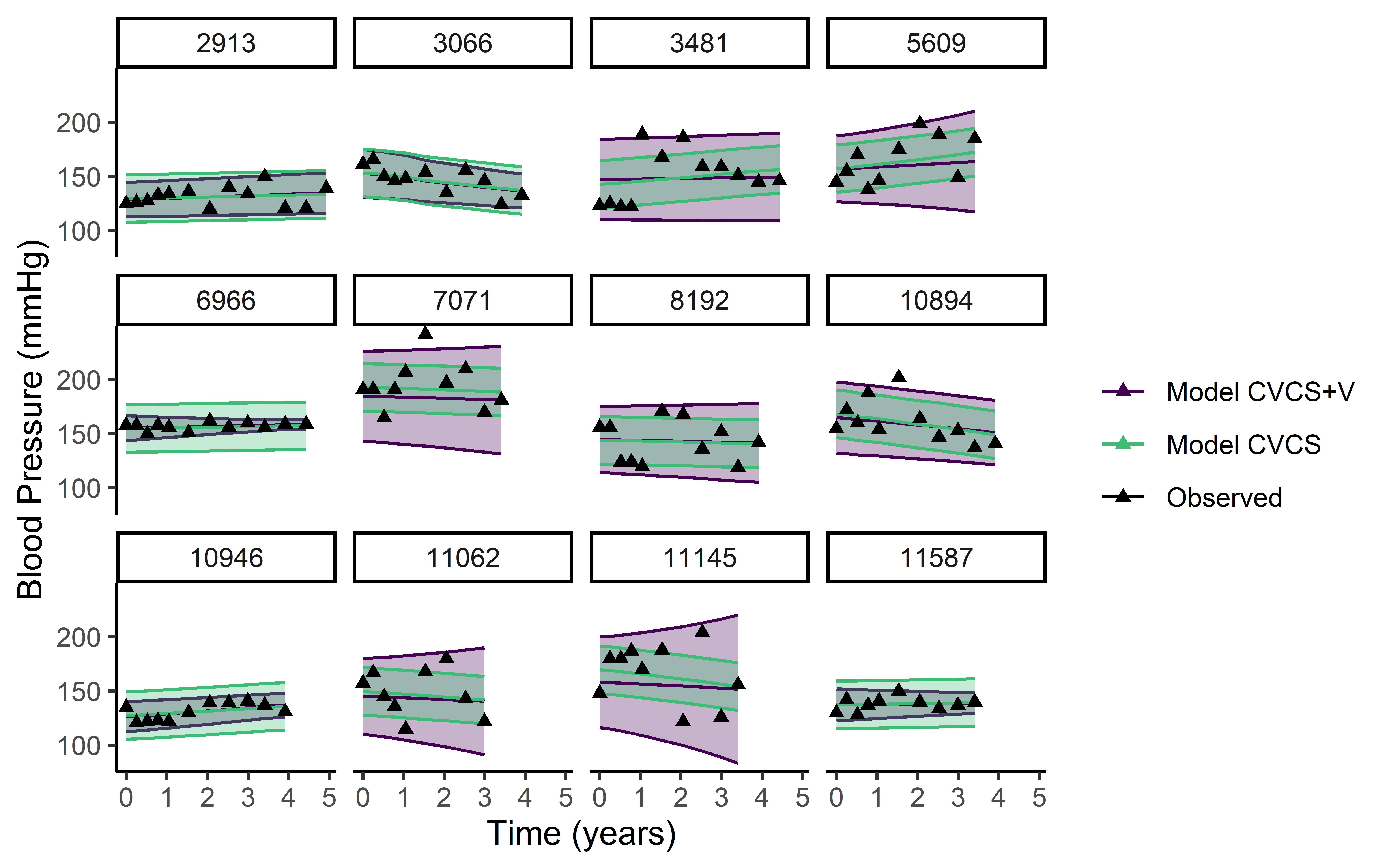
Figure 1: Prediction over time of the individual blood pressure and its prediction interval at 95% for 6 subjects. Model CVCS+V assumed a time-dependent subject-specific variability and the model CVCS assumes a homogeneous and constant variability. The black triangles are the observed measurements.

4.5 Predictions

We compared the predictive abilities of models with and without time-dependent individual variability using AUC in a 5-fold cross-validation. The individual predictions of having CVD (or death) between 3 and 4 years for subjects free of any event at 3 years were computed using equation (4). The AUC was computed using the timeROC package (Blanche et al., 2015). Although the AUCs are almost equal between models with and without heterogenous variability for the CVD risk (0.658 (0.015) and 0.655 (0.015), respectively), we obtained 0.704 (0.032) and 0.673 (0.033), respectively, for the risk of death. Between 3 and 5 years, the differences were larger in favour of our model but the standard errors were also higher due to the small number of patients still in the study at 5 years : 0.541 (0.063) and 0.515 (0.064) for the risk of CVD and 0.631 (0.077) and 0.604 (0.083) for the risk of death. These results suggest slightly better predictive abilities of the model accounting for the subject-specific residual variability.

To illustrate the effect of taking into account the current value of individual variance, we also computed the predicted risk of the events between 3 and 5 years for different subjects from both models, with and without time-dependent individual variability. We used the subjects selected for Figure 1 but model parameters used for computing the predicted probabilities were estimated without these subjects (using a cross-validation approach). Figures 2 and 3 shows that, for both the risk of CVD a,d the risk of death, the prediction is higher with the complete model when the individual experienced the event between 3 and 5 years than with the model without the heterogeneous variability. More, the predicted risk is smaller with the complete model when the individual do not experience the corresponding event.

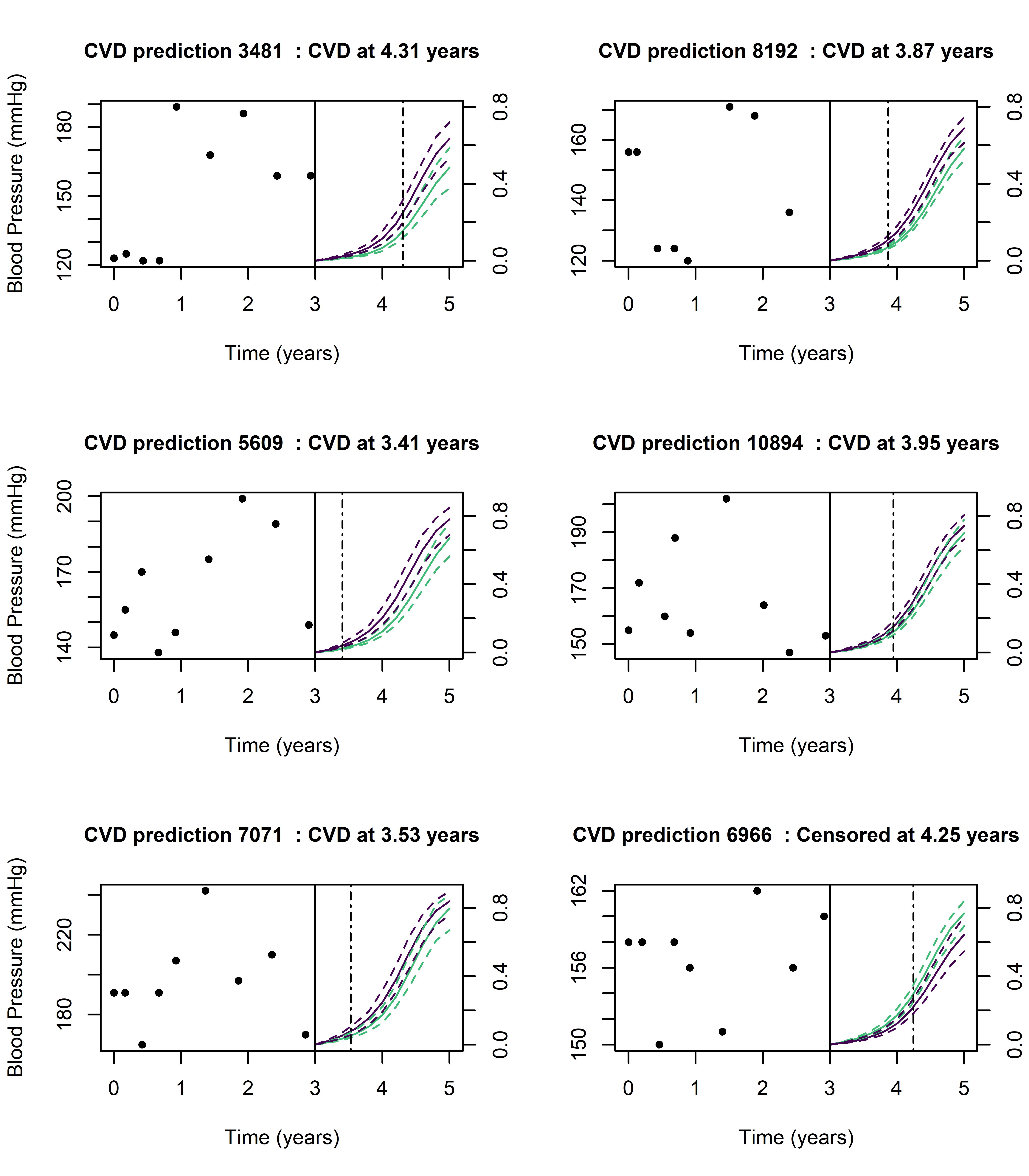
Figure 2: Prediction of the risk of CVD between 3 and 5 years (with its $95\%$ confidence interval indicated by dashed lines), for six patients at risk at 3 years, for Model CVCS+V (purple) and Model CVCS (green). The dashed lines represent the observed time.

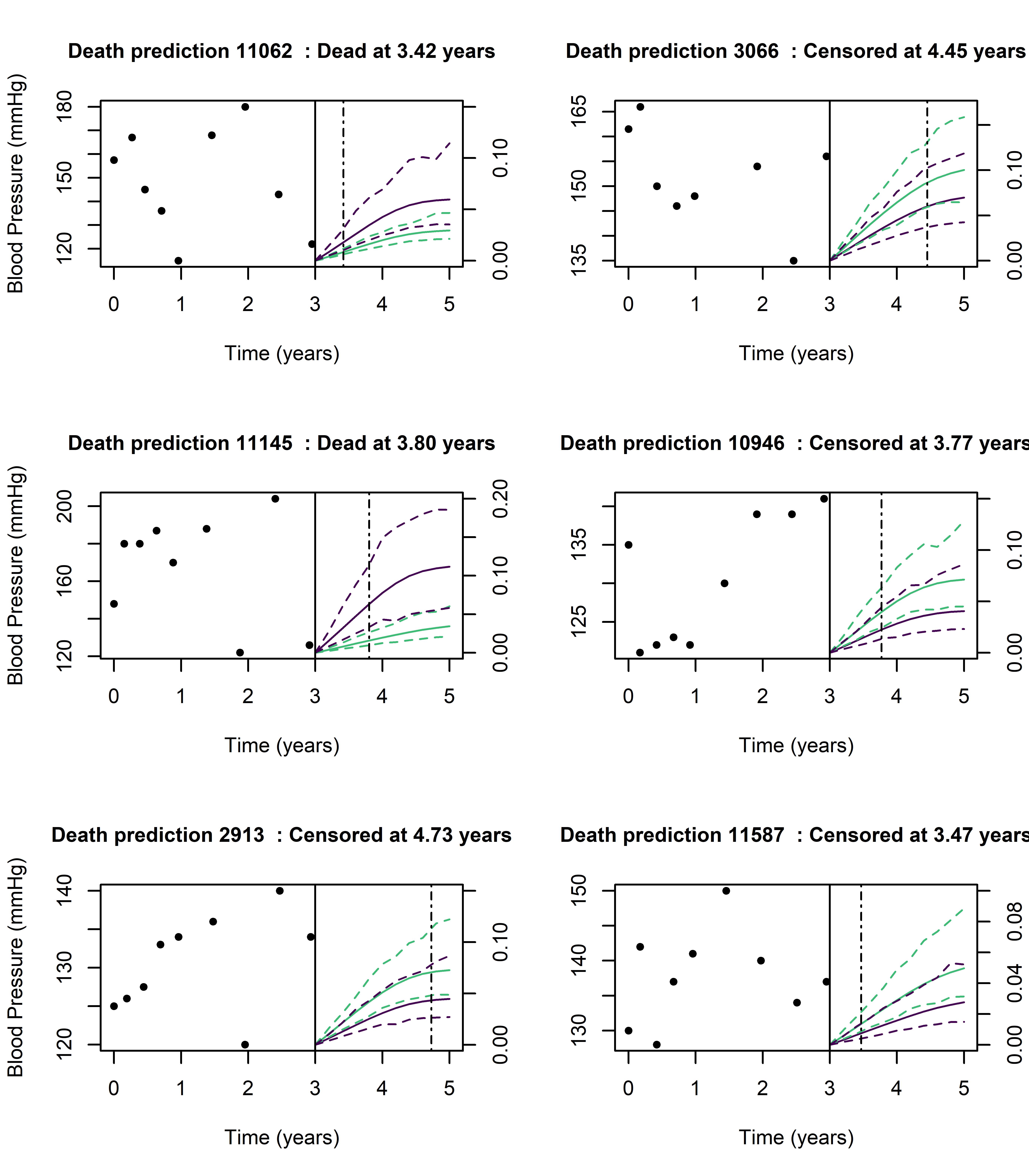
Figure 3: Prediction of the risk of Death between 3 and 5 years (with its $95\%$ confidence interval indicated by dashed lines), for six patients at risk at 3 years, for Model CVCS+V (purple) and Model CVCS (green). The dashed lines represent the observed time.

5 Discussion

In this work, we have proposed a new joint model with a subject-specific time-dependent variance that extends the models proposed by Gao et al. (Gao et al., 2011) and Barrett et al. (Barrett et al., 2019). Indeed, this new model allows time and covariate dependent individual variance and a flexible dependence structure between the competing events and the longitudinal marker. In particular, the risk of events may depend on both the current value and the current slope of the marker, in addition to the subject-specific time-dependent standard deviation of measurement errors. This is an important asset of the model given that, in most health research contexts, it is more sensible to assume that the event risk depends on the time-dependent current value or slope of the marker instead of only time-independent random effects. Moreover, accounting for competing events may be important in many clinical applications. In addition, we produced a R-package that allows frequentist estimation with a robust estimation algorithm which had shown very good behaviour in our simulations and in a previous work with different models (Philipps et al., 2021).
The analysis of the PROGRESS trial has shown that a high variability of blood pressure is associated with a high risk of CVD and death from other causes. Moreover, the individual residual variabily depends on time and treatment group.
In this work, we have supposed that the visit times were uninformative and missing measurements before the event were missing at random. In the PROGRESS clinical study, this hypothesis is quite plausible since visits were planed following a pre-specified protocol and the rate of missed visits before the event was low (less than $3\%$). For application to observational studies, it could be useful to extend this approach to consider an informative observation process. However, such a model would rely on non-verifiable parametric assumptions and could lead to identifiability issues.
Such joint models with dependence on the heterogeneous variance (that can be viewed as an extension of the location-scale mixed model (Hedeker and Nordgren, 1999)) are of great interest to investigate the association between the variability of markers or risk factors and the risk of health events in various fields of medical research. For instance, hypotheses have emerged about the link between emotional instability and the risk of psychiatric events, or the variability of glycemia and the prognosis of diabetes. Thanks to wearable devices, recent medical research studies often include frequent repeated measures of exposures or biomarkers, allowing the investigation of hypotheses regarding the variability.

Declaration of conflicting interests

The authors declared no potential conflicts of interest with respect to the research, authorship, and/or publication of this article.

Funding

This work was funded by the French National Research Agency (grant ANR-21-CE36 for the project "Joint Models for Epidemiology and Clinical research").
This PhD program is supported within the framework of the PIA3 (Investment for the Future). Project reference: 17-EURE-0019.

Additional simulation results

Table S1: Simulation results for scenario 1 with 1000 subjects.*

Parameter		True	Mean	Empirical	Mean asymptotic	Coverage
		value	estimate	SE	SE	rate (%)
Longitudinal submodel
Intercept	$\beta_{0}$	142	141.91	0.53	0.50	93.7
Slope	$\beta_{1}$	-0.1	-0.084	0.16	0.16	90.7
Variability	$\mu_{0}$	2.4	2.399	0.019	0.018	93.3
	$\mu_{1}$	-0.03	-0.031	0.009	0.009	92.3
Cholesky	$s_{0}$	14.5	14.61	0.43	0.36	88.0
	$s_{01}$	-1.2	-1.21	0.17	0.14	86.3
	$s_{1}$	2.8	2.81	0.12	0.10	91.7
	$s_{02}$	0.2	0.201	0.019	0.018	95.3
	$s_{12}$	-0.03	-0.031	0.021	0.023	94.3
	$s_{2}$	0.3	0.296	0.020	0.020	96.7
	$s_{03}$	-0.01	-0.010	0.009	0.008	92.3
	$s_{13}$	0.02	0.021	0.010	0.010	95.0
	$s_{23}$	-0.06	-0.057	0.012	0.012	93.3
	$s_{3}$	0.1	0.098	0.007	0.007	93.3
Survival submodel 1
Current variance	$\alpha_{\sigma 1}$	0.07	0.070	0.025	0.023	94.7
Current value	$\alpha_{11}$	0.005	0.0047	0.0054	0.0052	92.7
Current slope	$\alpha_{21}$	-0.07	-0.072	0.030	0.029	94.7
Weibull	$\sqrt{\kappa_{1}}$	1.6	1.596	0.037	0.037	94.7
	$\zeta_{01}$	-6	-5.95	0.67	0.65	94.7
Survival submodel 2
Current variance	$\alpha_{\sigma 2}$	0.15	0.150	0.030	0.030	94.0
Current value	$\alpha_{12}$	-0.01	-0.0099	0.0077	0.0072	92.3
Current slope	$\alpha_{22}$	-0.14	-0.141	0.045	0.042	93.7
Weibull	$\sqrt{\kappa_{2}}$	1.3	1.303	0.041	0.039	94.3
	$\zeta_{02}$	-4	-4.05	0.88	0.85	93.3

SE: Standard Error; Coverage rate: coverage rate of the $95\%$ confidence interval.
* Results for 300 replicates with complete convergence over 300.

Table S2: Simulation results for scenario 2 with 1000 subjects.*

Parameter		True	Mean	Empirical	Mean asymptotic	Coverage
		value	estimate	SE	SE	rate (%)
Longitudinal submodel
Intercept	$\beta_{0}$	142	141.93	0.53	0.50	95.0
Slope	$\beta_{1}$	3	3.02	0.17	0.17	95.6
Variability	$\mu_{0}$	2.4	2.40	0.02	0.02	93.6
	$\mu_{1}$	0.05	0.0496	0.0080	0.0079	94.0
Cholesky	$s_{0}$	14.5	14.59	0.43	0.37	90.3
	$s_{01}$	-1.2	-1.21	0.17	0.15	90.6
	$s_{1}$	2.8	2.79	0.12	0.11	92.3
	$s_{02}$	0.2	0.201	0.018	0.018	95.3
	$s_{12}$	-0.03	-0.031	0.022	0.024	95.3
	$s_{2}$	0.3	0.296	0.019	0.020	94.6
	$s_{03}$	-0.01	-0.010	0.008	0.008	93.6
	$s_{13}$	0.02	0.021	0.009	0.010	96.3
	$s_{23}$	-0.06	-0.058	0.011	0.011	95.6
	$s_{3}$	0.1	0.099	0.006	0.006	95.0
Survival submodel 1
Current variance	$\alpha_{\sigma 1}$	0.07	0.069	0.024	0.023	94.0
Current value	$\alpha_{11}$	0.02	0.0196	0.0067	0.0065	95.0
Current slope	$\alpha_{21}$	0.01	0.0094	0.0417	0.0408	95.3
Weibull	$\sqrt{\kappa_{1}}$	1.1	1.097	0.033	0.036	95.3
	$\zeta_{01}$	-7.0	-6.93	0.84	0.82	94.6
Survival submodel 2
Current variance	$\alpha_{\sigma 2}$	0.15	0.154	0.024	0.024	94.0
Current value	$\alpha_{12}$	-0.01	-0.0106	0.0075	0.0074	94.0
Current slope	$\alpha_{22}$	-0.14	-0.1399	0.0468	0.0439	94.6
Weibull	$\sqrt{\kappa_{2}}$	1.3	1.302	0.044	0.042	93.6
	$\zeta_{02}$	-4	-3.99	0.93	0.92	94.0

SE: Standard Error; Coverage rate: coverage rate of the $95\%$ confidence interval.
* Results for 298 replicates with complete convergence over 300.