Algorithms for Computing Maximum Cliques in Hyperbolic Random Graphs111This work was supported by the National Research Foundation of Korea(NRF) grant funded by the Korea government(MSIT) (No.RS-2023-00209069)
Abstract
In this paper, we study the maximum clique problem on hyperbolic random graphs. A hyperbolic random graph is a mathematical model for analyzing scale-free networks since it effectively explains the power-law degree distribution of scale-free networks. We propose a simple algorithm for finding a maximum clique in hyperbolic random graph. We first analyze the running time of our algorithm theoretically. We can compute a maximum clique on a hyperbolic random graph in expected time if a geometric representation is given or in expected time if a geometric representation is not given, where and denote the numbers of vertices and edges of , respectively, and denotes a parameter controlling the power-law exponent of the degree distribution of . Also, we implemented and evaluated our algorithm empirically. Our algorithm outperforms the previous algorithm [BFK18] practically and theoretically. Beyond the hyperbolic random graphs, we have experiment on real-world networks. For most of instances, we get large cliques close to the optimum solutions efficiently.
1 Introduction
Designing algorithms for analyzing large real-world networks such as social networks, World Wide Web, or biological networks is a fundamental problem in computer science that has attracted considerable attention in the last decades. To deal with this problem from the theoretical point of view, it is required to define a mathematical model for real-world networks. For this purpose, several models have been proposed. Those models are required to replicate the salient features of real-world networks. One of the most salient features of real-world networks is scale-free. In general, a graph is considered as a scale-free network if its diameter is small, one connected component has large size, it has subgraphs with large edge density, and most importantly, its degree distribution follows a power law. Here, for an integer , let be the fraction of nodes having degree exactly . If , we say that the degree distribution of the graph follows a power law. In this case, is called the power-law exponent.
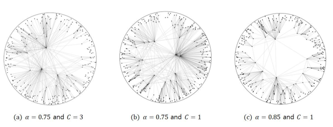
One promising model for scale-free real-world networks is the hyperbolic random graph model. A hyperbolic random graph is constructed from two parameters. First, points in the hyperbolic plane are chosen from a certain distribution depending on the parameters. Then we consider the points as the vertices of the constructed hyperbolic random graph. For two vertices whose distance is at most a certain threshold, we add an edge between them. For illustration, see Figure 1. It is known that the degree distribution of a hyperbolic random graph follows a power-law [16]. Moreover, its diameter is small with high probability [15, 17], and it has a giant connected component [10, 18]. Including these results, the structural properties of hyperbolic random graphs have been studied extensively [11]. However, only a few algorithmic results are known. In other words, the previous work focuses on why we can use hyperbolic random graphs as a promising model, but only a few work focuses on how to use this model for solving real-world problems. We focus on the latter type of problems.
In this paper, we focus on the maximum clique problem for hyperbolic random graphs from theoretical and practical point of view. The maximum clique problem asks for a maximum-cardinality set of pairwise adjacent vertices. For general graphs, this problem is NP-hard. Moreover, it is W[1]-hard when it is parameterized by the solution size, and it is APX-hard even for cubic graphs [2]. Therefore, the theoretical study on the clique problem focuses on special classes of graphs. In fact, this problem can be solved in polynomial time for special classes of graphs such as planar graphs, unit disk graphs and hyperbolic random graphs [7, 12, 14]. More specifically, the algorithm by Bläsius et al. [7] for computing a maximum clique of a hyperbolic random graph takes worst-case time. The randomness in the choice of vertices is not considered in the analysis of the algorithm. One natural question here is to design an algorithm for this problem with improved expected time.
To analyze our algorithm, we use the average-case analysis. A traditional modeling choice in the analysis of algorithms is worst-case analysis, where the performance of an algorithm is measured by the worst performance over all possible inputs. Although it is a useful framework in the analysis of algorithms, it does not take into account the distribution of inputs that an algorithm is likely to encounter in practice. It is possible that an algorithm performs well on most inputs, but poorly on a small number of inputs that are rarely encountered in practice. In this case, the worst-case analysis can mislead the analysis of algorithms. The field of ”beyond worst-case analysis” studies ways for overcoming these limitations [26]. One simple technique studied in this field is the average-case analysis. As the hyperbolic random graph model intrinsically defines an input distribution, the average-case analysis is a natural model for analyzing algorithms for hyperbolic random graphs.
Previous Work.
While the structural properties of hyperbolic random graphs has been studied extensively, only a few algorithmic problems have been studied. The most extensively studied algorithmic problem on hyperbolic random graphs is the generation problem: Given parameters, the goal is to generate a hyperbolic random graph efficiently. The best-known algorithms run in expected linear time [5] and in worst-case subquadratic time [27]. Also, Bläsius et al. [8] studied the problem of embedding a scale-free network into the hyperbolic plane and presented heuristics for this problem.
Very recently, classical algorithmic problems such as shortest path problems, the maximum clique problem and the independent set problem have been studied. These problems can be solved significantly faster in hyperbolic random graphs. More specifically, given a hyperbolic random graph, the shortest path between any two vertices can be computed in sublinear expected time [4, 9]. A hyperbolic random graph admits a sublinear-sized balanced separator with high probability [6]. As applications, Bläsius et al. [6] showed that the independent set problem admits a PTAS for hyperbolic random graphs, and the maximum matching problem admits a subquadratic-time algorithm. Also, the clique problem can be solved in polynomial time for hyperbolic random graphs in the worst case [7].
The clique problem has been studied extensively because it has numerous applications in various field such as community search in social networks, team formation in expert networks, gene expression and motif discovery in bioinformatics and anomaly detection in complex networks [20]. From a theoretical perspective, the best-known exact algorithm runs in time in [24]. However, it is not sufficiently fast for massive real-world networks, leading to the proposal of lots of exact algorithms and heuristics for this problem on real-world networks [1, 20, 22, 25]. While these algorithms and heuristics work efficiently in practice, there is no theoretical guarantee of their efficiency.
Our results.
We present algorithms for computing a maximum clique in a hyperbolic random graph and analyze their performances theoretically and empirically.
Given a hyperbolic random graph with parameters and together with its geometric representation, we can compute a maximum clique in expected time, where and denotes the numbers of vertices and edges of the given graph. Here, we have , and the O-notation hides a constant depending on and . With high probability, our algorithm outperforms the previously best-known algorithm by Bläsius et al. [7] running in time. In the case that a geometric representation is not given, our algorithm runs in expected time. This is the first algorithms for the maximum clique problem on hyperbolic random graphs not using geometric representations.
Also, we implemented our algorithms and analyzed it empirically. We run our algorithms on both synthetic data (hyperbolic random graphs) and real-world data. For hyperbolic random graphs, since it is proved that our algorithm computes a maximum clique correctly, we focus on the efficiency of the algorithms. We observed that our algorithms perform efficiently; it takes about 100ms for . For real-world networks, our algorithm gives a lower bound on the optimal solution. We observed that our algorithm performs well especially for collaboration networks and web networks. These are typical scale-free real-world networks.
2 Preliminaries
Let be the hyperbolic plane with curvature . We can handle hyperbolic planes with arbitrary (negative) curvatures by rescaling other model parameters which will be defined later. Thus it suffices to deal with the hyperbolic plane with curvature . Since the hyperbolic plane is isotropic, we choose an arbitrary point and consider it as the origin of . Also, we fix a half-line from going towards an arbitrary point, say , as the axis. Then we can represent a point of as where is the hyperbolic distance between and , and is the angle from to the half-line from going towards . We call and the radial and angular coordinates of .
For any two points and in , we use to denote the distance in between and . Then we have the following.
where denotes the small relative angle between and [3]. For a point and a value , we use to denote the disk centered at with radius . That is, .
2.1 Hyperbolic Random Graphs
A hyperbolic unit disk graph (HRG) is a graph whose vertices are placed on , and two vertices are connected by an edge if the distance between them on is at most some threshold. This threshold is called the radius threshold of the graph. This is the same as the unit disk graph except that the hyperbolic unit disk graph is defined on while the unit disk graph is defined on the Euclidean plane.
In this paper, we focus on the hyperbolic random graph model introduced by Papadopoulos et al. [21]. It is a family of distributions, indexed by the number of vertices, a parameter adjusting the average degree of a graph, and a parameter determining the power-law exponent. A sample from is a hyperbolic unit disk graph on points (vertices) chosen independently as follows. Let be the disk centered at with radius . To pick a point in , we first sample its radius , and then sample its angular coordinate . The probability density for the radial coordinate is defined as
| (1) |
Then the angular coordinate is sampled uniformly from . In this way, we can sample one vertex with respect to parameters and , and by choosing vertices independently and by computing the hyperbolic unit disk graph with radius threshold on the vertices, we can obtain a sample from the distribution .
An intuition behind the definition of is as follows. To choose a point uniformly at random in , we first choose its angular coordinate uniformly at random in as we did for , and choose its radial coordinate according to the distribution with density function . But in this case, the power-law exponent of a graph is fixed. To add the flexibility to the model, the authors of [21] introduced a parameter and defined the density function as in (1). Here, For , this favors points closer to the center of , while for , this favors points closer to the boundary of . For , this corresponds to the uniform distribution [16]. For illustration, see Figure 1.
Properties of HRGs.
Let be the probability measure of a set , that is,
For a vertex of a hyperbolic random graph with vertices, the expected degree of in is by construction. Moreover, notice that for any two vertices with . Thus to make the description easier, we let denote if it is clear from the context. Note that . For theoretical analyses of our algorithm, we analyze the probability measures for different sets using Lemma 1.
Lemma 1 ([7]).
For any , we have
where and are error terms which can be negligible (that is, ) if .
Hyperbolic random graphs have all properties for being considered as scale-free networks mentioned above. In particular, hyperbolic random graphs with parameter have power-law exponent , where if , and otherwise. Most real-world networks have a power-law exponent larger than two. Thus we assume that in the paper.
2.2 Algorithms for the Maximum Clique Problem
In this section, we review the algorithm for this problem on hyperbolic random graphs described in [7], which is an extension of [12]. This algorithms requires geometric representations of hyperbolic random graphs. Let be a hyperbolic random graph.
For , they showed that a hyperbolic random graph has maximal cliques with high probability. Therefore, a maximum clique can be computed in linear time with high probability by just enumerating all the maximal cliques.
For , they showed that the algorithm in [12] can be extended to hyperbolic random graphs. Assume first that, for a maximum clique , we have two vertices and of with maximum . Then all vertices in are contained in the region . Then we can compute by considering the vertices in as follows. We partition into and with respect to the line through and . They showed that the diameter of (and ) is at most one, and thus (and ) forms a clique. Therefore, the subgraph of induced by is the complement of a bipartite graph with bipartition . Moreover, is an independent set of the complement of . Therefore, it suffices to compute an independent set of the complement of , and we can do this in in time using the Hopcroft-Karp algorithm. However, we are not given the edge in advance. Thus we apply this procedure for every edge of , and then take the largest clique as a solution. This takes time in total.
Throughout this paper, we use to denote the probability that an event occurs. For a random variable , we use to denote the expected value of . We use the following form of Chernoff bound.
Theorem 2 (Chernoff Bound [13]).
Let be independent random variables with and let . Then we have
3 Efficient Algorithm for the Maximum Clique Problem
In this section, we present an algorithm for the maximum clique problem on a hyperbolic random graph drawn from running in expected time. This algorithm correctly works for any hyperbolic unit disk graph, but its time bound is guaranteed only for hyperbolic random graphs. As we only deal with the case that , this algorithm is significantly faster than the algorithm in [7].
A main observation is the following. A clique of size consists of vertices of degree at least . That is, to find a clique of size at least , removing vertices with degree less than does not affect the solution. Thus once we have a lower bound, say , on the size of a maximum clique, we can remove all vertices of degree less than . Our strategy is to construct a sufficiently large clique (which is not necessarily maximum) as a preprocessing step so that we can remove a sufficiently large number of vertices of small degree. After applying a preprocessing step, we will see that the number of vertices we have decreases to with high probability. Then we apply the algorithm in [7] to the resulting graph.
3.1 Computing a Sufficiently Large Clique Efficiently
In this section, we show how to compute a clique of size with probability . The algorithm is simple: Scan the vertices in the non-increasing order of their degrees, and maintain a clique , which is initially set as . If the next vertex can be added to to form a larger clique, then add it, otherwise exclude it. We can sort the vertices with respect to their degrees in time using counting sort. Also, we can construct the clique in time. In the following, we call the initial clique.
Now, we show that the size of the initial clique is with probability . First, we show that a sufficient large clique can be found by collecting all vertices in with high probability in Lemma 3.
Lemma 3.
For any constant , the vertices in forms a clique of size with probability .
Proof. For any two vertices and in , we have
That is, and are connected by an edge. Therefore, the vertices in form a clique.
Now we show that the number of vertices in is at most with high probability. For this purpose, we define a random variable as the number of vertices in . Then by Lemma 1, we have
Applying , we have
for some constant . By Chernoff bound, we have
for any constant .
Thus, we can get desired clique by choosing vertices in with high probability. However, as we scan the vertices in the decreasing order of their degrees, this does not immediately imply that the size of the initial clique is . In the following lemma, we show that the initial clique has the claimed size by showing that the vertices with highest degrees are contained in with high probability.
Lemma 4.
The initial clique has size with probability .
Proof. First, we show that no vertex lying outside of has degree greater than with high probability for some constant which will be defined later. For this purpose, we analyze the expected degree of a vertex whose radius coordinate is larger than . Let be the degree of . Then we have
for . By applying , we have
for . By Chernoff bound, we have
Therefore, the probability that all vertices lying outside of have degree larger than is at most . In other words, there is no vertex of degree greater than in with probability .
Now we show that no vertex in has degree smaller than with high probability for some constant which will be specified later. For this purpose, we analyze the probability that a vertex in has degree smaller than . Let be the degree of . Then we have
Here, is the constant we used for the previous case. By Chernoff bound, we have
for any constant . By choosing , we get
Therefore, the probability that all vertices contained in have degree smaller than is at most . In other words, there is no vertex of degree smaller than in with probability .
To construct the initial solution, we scan the vertices in the decreasing order of their degrees. Therefore, with probability , we consider all vertices in before considering any vertex lying outside of . Therefore, the initial clique contains all vertices in with high probability. By Lemma 3, the initial clique has size at least with high probability.
3.2 Removing All Vertices of Small Degree
In this section, we show how to remove a sufficiently large number of vertices, and show that the size of the remaining graph is with high probability. This algorithm is also simple: given the initial clique of size , we repeatedly delete all vertices of degree smaller than . We call the resulting graph the kernel. Then no vertex in the kernel has degree smaller than at the end of the process. This process can be implemented in linear time as follows: maintain the queue of vertices of degree smaller than , and maintain the degree of each vertex. Then remove the vertices in the queue in order. Whenever a vertex is removed, update the degree of each neighbor of and insert to the queue if its degree gets smaller than .
We show that the kernel has size . Notice that we do not specify the order of vertices we consider during the deletion process. Fortunately, the kernel size remains the same regardless of the choice of deletion ordering.
Lemma 5.
In any order of deleting vertices, we can get a unique kernel.
Proof. Let be a given graph. Let and be two different sequences of vertices deleted during the deletion process. We first show that a set contains . If , the degree of in is less than because removing vertices does not increase the degree of , where denotes the subgraph of induced by a vertex set . That is, if , the deletion process would not terminate for , and thus we conclude that . Inductively, assume that . If , the degree of in is at most the degree of in , and thus the degree of in is less than . Then the deletion process would not terminate for , and thus . Therefore, we have . Symmetrically, we can also show that , and thus . Therefore, the any order of deleting vertices gives the same remaining vertices.
Because of the uniqueness of the kernel, for analysis, we may fix a specific deletion ordering and slightly modify the deletion process as follows. Imagine that we scan the vertices in the decreasing order of their radial coordinates. If the degree of a current vertex (in the remaining graph) is at least the size of the initial clique size, then we terminate the deletion process. Otherwise, we delete the current vertex, and consider the next vertex. By Lemma 5, the number of remaining vertices is at least the size of the kernel. In the following lemma, we analyze the number of remaining vertices.
Lemma 6.
Given an initial solution of size , then the size of the kernel is with probability .
Proof. Let be a sufficiently small constant such that the size of the initial solution is at least . Let be the radius satisfying . By choosing as a sufficient small constant, we may assume that . In the following, we show that all the vertices with radial coordinates larger than are removed with probability . Observe that is decreasing for . That is, for ,
For a vertex , we define the inner degree of as the number of its neighboring vertices whose radial coordinates are smaller than the radial coordinate of . Let be the inner degree of . Then the expected inner degree of a vertex with radial coordinate is as follows.
By Chernoff bound,
Therefore, for a vertex with radial coordinate larger than , the probability that its inner degree is larger than the size of the initial clique is at most . By the union bound over at most vertices with radial coordinates larger than , the probability that no vertex with radial coordinate larger than has inner degree larger than than the size of the initial clique is at most . In other words, with probability , all vertices with radial coordinates larger than have inner degree larger than the size of the initial clique.
If this event happens, we remove all vertices with coordinates larger than . Therefore, it suffices to show that the number of vertices with coordinates at most is small. The expected number of such vertices is . For this, we obtain the explicit formula for as follows. From , we get
Applying , we obtain
Let be the number of vertices lying inside . Then the expected number of vertices we have after applying the deletion process is as follows.
Therefore,
for some constant depending only on and . By Chernoff bound,
In summary, with probability , all vertices with radial coordinates larger than have inner degree larger than the size of the initial clique. Also, with probability , the number of vertices in is at most . Therefore, the probability that the number of remaining vertices after applying the deletion process is at most is at least , which is .
Although the deletion process we use for analysis requires the geometric representation of , the original deletion process does not require the geometric representation of . By combining the argument in Section 3.1 and Section 3.2, we have the following theorem.
Theorem 7.
Given a graph drawn from with and its geometric representation, we can compute its maximum clique in expected time.
Proof. We first show its maximum clique can be computed in time with probability at least . We can compute the initial solution of size in time with probability . Then we apply the algorithm in [7] to the initial solution for computing a maximum clique of a hyperbolic random graph with vertices and edges in time. Since in the worst case, the total running time is .
Even in the case that the reduction fails to delete a sufficient number of vertices, the running time of the algorithm is . Thus the expected running time is
4 Efficient Robust Algorithm for the Maximum Clique Problem
In this section, we present the first algorithm for the maximum clique problem on hyperbolic random graphs which does not require geometric representations. In many cases, a geometric representation of a graph is not given. In particular, real-world networks such as social and collaboration networks are not defined based on geometry although they share properties with HRGs. As we want to use hyperbolic random graphs as a model for such real-world networks, it is necessary to design algorithms not requiring geometric representations.
Our main key tool in this section is the notion of co-bipartite neighborhood edge elimination ordering (CNEEO) introduced by Raghavan and Spinrad [23]. It can be considered as a variant of a perfect elimination ordering. Let be an undirected graph. Let be an edge ordering of all edges of . Let be the subgraph of with the edge set . For a vertex , let denote the set of neighbors of in . Then is called a co-bipartite neighborhood edge elimination ordering (CNEEO) if for each edge , the subgraph of induced by is co-bipartite. Here, a co-bipartite graph is a graph whose complement is bipartite.
Raghavan and Spinrad [23] presented an algorithm for computing a CNEEO in polynomial time if a given graph admits a CNEEO. Moreover, they presented a polynomial-time algorithm for computing a maximum clique in polynomial time assuming a CNEEO is given. We first show that a hyperbolic unit disk graph admits a CNEEO. This immediately leads to a polynomial-time algorithm for the maximum clique problem.
Lemma 8.
Every hyperbolic unit disk graph admits a CNEEO.
Proof. Let be a hyperbolic unit disk graph, and be the ordered set of all edges in sorted in the non-increasing order of their lengths. For each edge , and for all . Thus the vertices in are contained in with . Because the subgraph of induced by the vertices in is co-bipartite, the subgraph of induced by is also co-bipartite. Thus, is the CNEEO.
Since Raghavan and Spinrad [23] did not give an explicit time bound on their algorithm, we describe their algorithm and analyze their running time in the following lemma. Note that the following lemma holds for an arbitrary graph (not necessarily a hyperbolic unit disk graph) admitting a CNEEO.
Lemma 9 ([23]).
Given a graph which admits a CNEEO, the maximum clique problem can be solved in time.
Proof. If has a CNEEO, we can compute it in a greedy fashion in time. Starting with an empty ordering, we add edges to the ordering one by one. At each step , we have an ordering , and we extend this ordering by adding an edge. Let be the subgraph of induced by . Then for each edge , we check if the common neighbors of its endpoints in induces a co-bipartite graph in . If so, we add it at the end of the current ordering. If has a CNEEO, Raghavan and Spinrad [23] showed that this greedy algorithm always returns a CNEEO. For its analysis, observe that we have steps. For each step , the number of candidates for is , and for each candidate , we can check if the common neighbors of its endpoints induces a co-bipartite graph in time. To see this, observe that cannot be co-bipartite if . Thus if the number of edges of is at least , we can immediately conclude that cannot be the th edge in the ordering. Otherwise, we can check if is co-bipartite in time, which is at most time. In this way, we can complete each step in time, and thus the total running time is .
Then using the CNEEO, we can compute a maximum clique as follows. For each , we compute a maximum clique of the subgraph of induced by . Since it is co-bipartite, it is equivalent to computing a maximum independent set of its complement, which is bipartite. This takes time using the Hopcroft-Karp algorithm. Raghavan and Spinrad [23] showed that a largest clique among all such cliques is a maximum clique of . Thus, we can find maximum clique of in .
In the case of hyperbolic random graphs, we can solve the problem even faster. As we did in Section 3, we compute an initial clique, remove vertices of small degrees, and then obtain a kernel of small size. Recall that these procedures do not require geometric representations. Note that the kernel is also a hyperbolic unit disk graph because we remove vertices only. The number of vertices of the kernel is and the edges is in probability . Thus, we have the following theorem.
Corollary 10.
Given a graph drawn from with , we can compute a maximum clique in expected time without its geometric representation.
Heuristics for real-world networks.
A main motivation of the study of hyperbolic random graphs is to obtain heuristics for analyzing real-world networks. Many real-world networks share salient features with hyperbolic random graphs, but this does not mean that many real-world networks are hyperbolic random graphs. Because the algorithm in Corollary 10 is aborted for a graph not admitting a CNEEO, one cannot expect that this algorithm works correctly for many real-world networks. In fact, only a few real-world networks admit CNEEO as we will see in Section 6. That is, for most of real-world networks, the algorithm in Corollary 10 is aborted.
However, in this case, we can obtain a lower bound on the optimal clique sizes, and moreover, we can reduce the size of the graph.
Lemma 11.
Assume that the algorithm in Theorem 10 is aborted at step . Let be the ordering we have at stage . For an index , let be the subgraph of with edge set . Then either a maximum clique of is a maximum clique of , or a maximum clique of the subgraph of induced by the common neighbors of the endpoints of tin is a maximum clique of for some index .
Proof. Let be a maximum clique of . If an edge of the ordering we have at stage has both endpoints in , let be the first edge in the ordering among them. In this case, is a clique of the subgraph induced by the common neighbors of the endpoints of in . To see this, observe that all vertices of are common neighbors of the endpoints of , and they are vertices in . Therefore, a maximum clique of has size , and thus the lemma follows.
If no edge of the ordering we have at stage has both endpoints in , then is a clique in . Therefore, it belongs to the first case described in the statement of the lemma. Therefore, the lemma holds for any case.
Although we do not have any theoretical bound here, our experiments showed that the size of the clique we can obtain is close to the optimal value for many instances. Details will be described in Section 6.
5 Improving Performance through Additional Optimizations
For implementation, we introduce the following two minor techniques for improving the performance of the algorithms. Although these techniques do not improve the performance theoretically, they improve the performance empirically. Recall that our algorithms consist of two phases: Computing a kernel of size , and then computing a maximum clique of the kernel. As the first phase can be implemented efficiently, we focus on the second phase here. Again, the second phase has two steps. With geometric representations, we first compute a CNEEO, and then compute a maximum clique using the CNEEO. Without geometric representations, we consider every edge, and then compute a maximum clique in the subgraph induced by the common neighbors of the endpoint of the edge. The first technique applies to both of the two steps, and the second technique applies to the first step.
5.1 Skipping Vertices with Low Degree
The main observation of our kernelization algorithm is that, for any lower bound on the size of a maximum clique, a vertex of degree less than does not participate in a maximum clique. The first technique we use in the implementation is to make use of this observation also for computing a CNEEO, and for computing a maximum clique using the CNEEO.
While computing a CNEEO, the lower bound we have does not change; it is the size of the initial clique. Whenever we access a vertex, we check if its degree is less than . If so, we remove this vertex from the kernel, and do not consider it any more. One can consider this as “lazy deletion.” Then once we have a CNEEO, we scan the edges in the CNEEO, and for each edge, we compute a maximum clique of the subgraph defined by the edge. If it is larger than the lower bound we have, we update accordingly. In this process, whenever we find a vertex of degree less than , we remove it immediately. Moreover, if the subgraph defined by each edge of CNEEO has vertices less than , we skip this subgraph as it does not contain a clique of size larger than .
5.2 Introducing the Priority of Edges
Recall that the second phases consists of two steps: computing a CNEEO, and computing a maximum clique using the CNEEO. In this section, we focus on the first step.
With Geometric Representations.
In this case, we use the -time algorithm by [7] for computing a maximum clique of the kernel with vertices and edges. Although it is the theoretically best-known algorithm, we observed that computing a maximum clique using a CNEEO is more efficient practically. By the proof in lemma 8, the list of the edges sorted in the non-decreasing order of their lengths is a CNEEO. Without using a CNEEO, for each edge , we have to compute the subgraph of induced by the common neighbors of and in . On the other hand, once we have a CNEEO, it suffices to consider the subgraph of induced by the common neighbors of and in , where is the subgraph of with the edges coming after in the CNEEO. If lies close to the last edge in the CNEEO, the number of common neighbors of and in can be significantly smaller than the number of their common neighbors in . This can lead to the performance improvement.
Without Geometric Representations.
In this case, we compute a CNEEO in a greedy fashion. Starting from the empty sequence, we add the edges one by one in order. For each edge not added to the current ordering, we check if the common neighbors of the endpoints of in the kernel is co-bipartite. If an edge passes this test, we add it to the ordering. It is time-consuming especially when only a few edges can pass the test. To avoid considering the same edge repeatedly, we use the following observation. Once an edge fails this test, it cannot pass the test unless one of its incident edges are added to the ordering. Using this observation, we classify the edges into two sets: active edges and inactive edges. In each iteration, we consider the active edges only. Once an edge fails the test, then it becomes inactive. Once an edge passes the test, we make all its incident edges active. In this way, we can significantly improve the running time especially for graphs that do not accept CNEEO.
6 Experimental Evaluation
In this section, we evaluate the performance of our algorithm mainly on hyperbolic random graphs and real-world networks.
Environment and data.
We implemented our algorithm using C++17. The code were compiled with GNU GCC version with optimization flag ”-O2”. All tests were run on a desktop with Rygen 7 3800X CPU, 32GB memory, and Ubuntu 22.04LTS.
We evaluate the performance of our algorithm on hyperbolic random graphs and real-world networks. For hyperbolic random graphs, we generate graphs using the open source library GIRGs [5] by setting parameters differently. Recall that we have three parameters , and . Here, instead of , we use the average degree, denoted by , as a parameter because can be represented as a function of and . As we consider the average performance of our algorithm, we sampled 100 random graphs for fixed parameters and , and then calculate the average results (the size of kernels or the running times).
For real-world networks, we use the SNAP dataset [19]. It contains directed graphs and non-simple graphs as well. In this case, we simply ignore the directions of the edges and interpret all directed graphs as undirected graphs. Also, we collapse all multiple edges into a single edge and remove all loops.
6.1 Experiment on Hyperbolic Random Graphs: Kernel Size
We showed that the size of the kernel of the hyperbolic random graph is with probability . In this section, we evaluated the tendency on the size of the kernel experimentally as , and change. Here, controls the power-law exponent, and is the average degree of the graph.
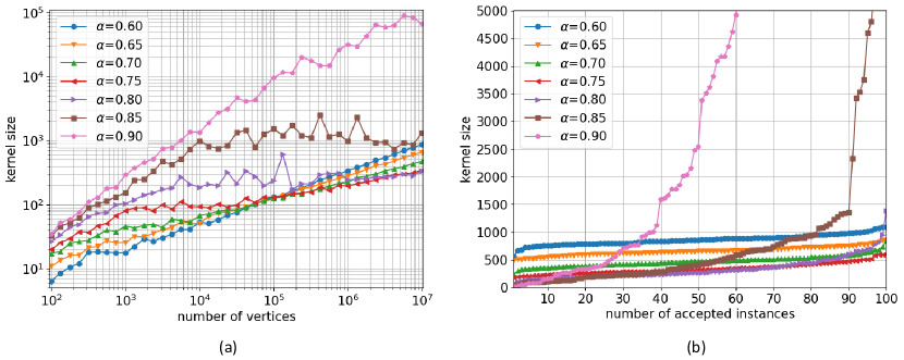
Figure 2 shows the tendency on the size of the kernel as changes. Here, we fix . Figure 2(a) shows a plot of the kernel size versus the number of vertices of a graph on a log–log scale for each value of . We generate 100 instances randomly and take the average of their results for each point in the plot. Figure 2(b) shows a cactus plot of the kernel size versus the number of accepted instances for each value of . Here, for a fixed kernel size , an instance is said to accepted if our algorithm returns a kernel of size at most for this instance. Here, we fix and .
For , the size of the average kernel decreases for sufficiently large , say , as increases in Figure 2(a). Also, the kernel sizes for all instances are concentrated on the average kernel size for each in Figure 2(b). This is consistent with Lemma 6 stating that the kernel size is with high probability. However, this fact does not hold for in Figure 2(a), and the reason for this can be seen in Figure 2(b). At , approximately of instances did not have kernels of size at most , and at , over of instances did not have such kernels. Notice that the plot sharply increases when the kernel size exceeds . The success probability stated in Lemma 6 is , which decreases as increases. In other words, if is not sufficiently large, it is possible that the success probability is not sufficiently large for . That is, if we increase the number of vertices on our experiments, we would get the desired tendency on the kernel size for all values . Nevertheless, at , our algorithm removes a significant number of vertices, leaving only of vertices at and only at .
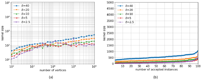
Figure 3(a) shows that the kernel size increases as increases. Here, we fix . Figure 3(b) shows a cactus plot of the kernel size versus the number of accepted instances for each value of . The kernel sizes for all instances are concentrated on the average kernel size for each . This tendency can be explained from the proof of Lemma 6. The constant hidden behind the O-notation in the lemma depends on , and thus it also depends on . By carefully analyzing this constant, we can show that the average kernel size increases as increases (for a fixed .) Similarly, we can show that the success probability increases as increases.
6.2 Experiment on Hyperbolic Random Graphs: Running Time
| INIT | KERNEL | CNEEO | CONST | INDEP | OTHER | TOTAL | |
|---|---|---|---|---|---|---|---|
| MaxClique | - | - | - | 21 516.34 | 4 470.38 | 8.18 | 25 994.90 |
| MaxCliqueRed | 15.67 | 89.27 | - | 1 126.95 | 37.92 | 2.88 | 1 272.70 |
| MaxCliqueSkip | 15.59 | 88.62 | - | 925.33 | 30.77 | 2.88 | 1 063.19 |
| MaxCliqueOpt | 15.64 | 88.61 | 1.07 | 12.55 | 1.19 | 2.88 | 121.94 |
| MaxCliqueNoGeo | 15.32 | 89.25 | 258.45 | 5.82 | 0.93 | 2.96 | 372.74 |
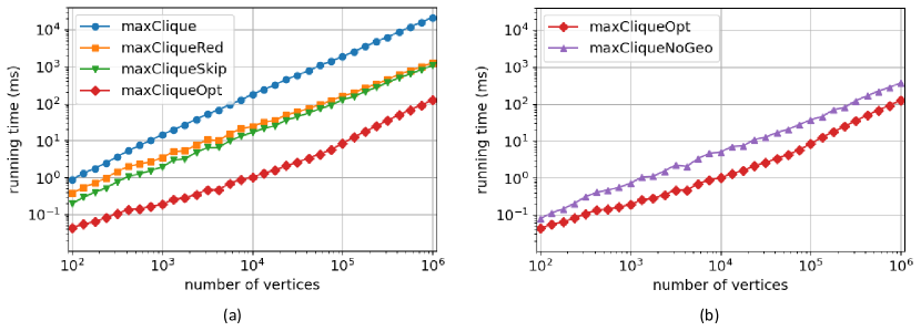
In this section, we conducted experiments for evaluating the running times of different versions of our algorithms. Figure 4 shows a plot of the number of vertices versus the running time of each version of our algorithm. Here, we fix and . Each point of the plot is averaged for instances. Figure 4(a) shows a plot for the algorithm, denoted by MaxClique, by Bläsius et al. [7] and three different versions of the algorithm using geometric representations: MaxCliqueRed, MaxCliqueSkip, and MaxCliqueOpt. More specifically, MaxCliqueRed denotes the algorithm described in Section 4. MaxCliqueSkip denotes the algorithm described in Section 5.1 that skips low-degree vertices. MaxCliqueOpt denotes the algorithm described in Section 5.2 that introduces priorities of edges. As expected, MaxCliqueOpt outperforms all other versions of the algorithms in this experiment.
For a precise analysis, we evaluated the running time of each task for our algorithms and reported them in in Table 1. More specifically, the algorithms conduct six tasks: INIT denotes the task of finding an initial solution. KERNEL denotes the task of finding the kernel. CNEEO denotes the task of computing a CNEEO. CONST denotes the task of constructing a co-bipartite graph by considering the common neighbors of the endpoints of each edge. INDEP denotes the task of computing a maximum independent set of the complement of a co-bipartite graph. OTHER denotes all the other tasks such as the initialization for variables and caches. TOTAL denotes the entire tasks of our algorithm.
As expected, MaxCliqueRed outperforms MaxClique significantly. However, CONST is still a time-consuming task for MaxCliqueRed. Thus we focus on optimization techniques for CONST and provides MaxCliqueSkip and MaxCliqueOpt in Section 5. Although MaxCliqueSkip gives a performance improvement, it still takes a significant amount of time in CONST and INDEP. MaxCliqueOpt computes a CNEEO by sorting the edges with respect to their lengths. This allows us to manage degree efficiently and apply low-degree skip technique to a larger number of vertices. This significantly improves the running time of MaxCliqueSkip for CONST and INDEP. This algorithm runs in about ms even at , exhibiting a performance improvement over times compared to MaxClique.
Next, we compared the running times of two algorithms with and without geometrical representations. In the case that a geometric representation is given, we use MaxCliqueOpt. If a geometric representation is not given, we use the algorithm in Section 4 and denote it by MaxCliqueNoGeo. In MaxCliqueOpt, we can quickly compute a CNEEO by sorting the edges in non-decreasing order of length. However, MaxCliqueNoGeo computes a CNEEO in a greedy approach which incurs significant overhead. Despite this, the performance of MaxCliqueNoGeo in Figure 4(b) does not show a significant difference compared to MaxCliqueOpt, and it even outperforms MaxCliqueSkip.
| runtime | |||||||||
|---|---|---|---|---|---|---|---|---|---|
| as-skitter | 1 696,415 | 11 095,298 | 28 787 | 17 033 | 693 272 | 342.63 | 37 | 63 | 67 |
| ca-AstroPh | 18 771 | 198 050 | 3 679 | 0 | 0 | 1.18 | 23 | 57 | 57 |
| ca-CondMat | 23 133 | 93 439 | 13 464 | 0 | 0 | 0.07 | 4 | 26 | 26 |
| ca-HepPh | 11 204 | 118 489 | 0 | 0 | 0 | 0.00 | 239 | 239 | 239 |
| com-amazon | 334 863 | 925 872 | 255 473 | 0 | 0 | 0.55 | 3 | 7 | 7 |
| com-dblp | 317 080 | 1 049 866 | 1 716 | 0 | 0 | 0.21 | 26 | 114 | 114 |
| com-lj | 3 997 962 | 34 681 189 | 1 713 237 | 126 388 | 4 587 418 | 2 316.20 | 7 | 289 | 327 |
| com-youtube | 1 134 890 | 2 990 443 | 36 716 | 7 919 | 211 051 | 53.48 | 13 | 14 | 17 |
| Gnutella31 | 62 586 | 147 892 | 33 816 | 0 | 0 | 0.05 | 2 | 4 | 4 |
| Slashdot0811 | 77 360 | 469 180 | 14 315 | 1 503 | 40 418 | 7.94 | 10 | 17 | 26 |
| Slashdot0902 | 82 168 | 504 229 | 13 964 | 1 543 | 42 215 | 9.24 | 11 | 17 | 27 |
| soc-Epinions1 | 75 879 | 405 740 | 9 337 | 3 717 | 148 354 | 26.09 | 10 | 22 | 23 |
| soc-pokec | 1 632 803 | 22 301 964 | 1 252 317 | 54 101 | 924 531 | 288.37 | 4 | 29 | 29 |
| web-BerkStan | 685 230 | 6 649 470 | 27 058 | 25 593 | 589 913 | 1 224.22 | 18 | 201 | 201 |
| web-Google | 875 713 | 4 322 051 | 193 406 | 2 068 | 20 426 | 8.60 | 10 | 44 | 44 |
| web-NotreDame | 325 729 | 1 090 108 | 51 227 | 760 | 8 181 | 4.86 | 6 | 155 | 155 |
| web-Stanford | 281 903 | 1 992 636 | 32 123 | 10 721 | 249 272 | 177.79 | 18 | 61 | 61 |
| WikiTalk | 2,394 385 | 4 659 563 | 70 130 | 10 421 | 520 338 | 447.69 | 7 | 16 | 26 |
| Wiki-Vote | 7 115 | 100 762 | 2 913 | 1 802 | 62 893 | 6.34 | 9 | 13 | 17 |
6.3 Experiment on Real-World Dataset
Our algorithm can heuristically find large cliques for real-world data. We conducted experiments on several real-world datasets and recorded these results in Table 2. The unit of the running time is a second. and denote the numbers of vertices and edges of the input graph, respectively. denotes the number of vertices of the kernel. and denote the numbers of vertices and edges of the remaining graph described in Lemma 11, respectively. Also, denotes the size of the initial clique, denotes the size of the clique computed from our algorithm, and denotes the size of the maximum clique of the graph. Here, is the correct answer given by the dataset. If a given graph accepts a CNEEO, it is theoretically guaranteed that is the exact solution and . Otherwise, is a lower bound on the exact solution by Lemma 11, and has a maximum clique if is strictly smaller than the exact solution.
The collaboration networks such as ca-AstroPh, CondMat, HepPh, and com-dblp are one of the well-known scale-free networks. These networks accept a CNEEO, allowing us to find the exact maximum clique. Moreover, we were able to find a CNEEO considerably faster for these networks than for other graphs in our experiments. Web graphs such as web-BerkStan, web-Google, web-Notre Dame, and web-Stanford are also one of the well-known scale-free networks. Although these graphs do not accept a CNEEO, we were able to reduce the number of vertices and edges significantly, and we obtained maximum cliques. For the other graphs we tested, we were able to obtain lower bounds that were close to the maximum clique size in most cases, and we were able to significantly reduce the size of the graphs.
7 Conclusion
We presented improved algorithms for the maximum clique problem on hyperbolic random graphs. Our algorithms find a sufficiently large initial solution and find a sufficiently small kernel in linear time, which greatly improves the average time complexity and practical running time. Also we gave the first algorithm for the maximum clique problem on hyperbolic random graphs without geometrical representations. Beyond the hyperbolic random graph, we applied these algorithms to real-world dataset and obtained lower bounds close to the optimum solutions for most of instances.
There are two possible directions for further improvement on our algorithms. First, we compute a maximum clique of hyperbolic random graphs using the framework for computing a maximum clique of unit disk graphs in [12]. Recently, Espenant et al. [14] improved the algorithm [12] and presented an -time algorithm for the maximum clique problem on unit disk graphs. It would be interesting if this technique can be applied to hyperbolic geometry. Second, the bottleneck of our algorithm lies in constructing a CNEEO. Especially, for most of real-world dataset, most of the running time is devoted to constructing a CNEEO. Thus to speed up the overall performance, this step must be improved.
References
- [1] James Abello, Mauricio GC Resende, and Sandra Sudarsky. Massive quasi-clique detection. In LATIN 2002: Theoretical Informatics: 5th Latin American Symposium Cancun, Mexico, April 3–6, 2002 Proceedings 5, pages 598–612. Springer, 2002.
- [2] Paola Alimonti and Viggo Kann. Some APX-completeness results for cubic graphs. Theoretical Computer Science, 237(1-2):123–134, 2000.
- [3] James W Anderson. Hyperbolic geometry. Springer Science & Business Media, 2006.
- [4] Thomas Bläsius, Cedric Freiberger, Tobias Friedrich, Maximilian Katzmann, Felix Montenegro-Retana, and Marianne Thieffry. Efficient shortest paths in scale-free networks with underlying hyperbolic geometry. ACM Transactions on Algorithms (TALG), 18(2):1–32, 2022.
- [5] Thomas Bläsius, Tobias Friedrich, Maximilian Katzmann, Ulrich Meyer, Manuel Penschuck, and Christopher Weyand. Efficiently generating geometric inhomogeneous and hyperbolic random graphs. Network Science, 10(4):361–380, 2022.
- [6] Thomas Bläsius, Tobias Friedrich, and Anton Krohmer. Hyperbolic random graphs: Separators and treewidth. In 24th Annual European Symposium on Algorithms (ESA 2016). Schloss Dagstuhl-Leibniz-Zentrum fuer Informatik, 2016.
- [7] Thomas Bläsius, Tobias Friedrich, and Anton Krohmer. Cliques in hyperbolic random graphs. Algorithmica, 80(8):2324–2344, 2018.
- [8] Thomas Bläsius, Tobias Friedrich, Anton Krohmer, and Sören Laue. Efficient embedding of scale-free graphs in the hyperbolic plane. IEEE/ACM transactions on Networking, 26(2):920–933, 2018.
- [9] Thomas Bläsius, Tobias Friedrich, and Christopher Weyand. Efficiently computing maximum flows in scale-free networks. In 29th Annual European Symposium on Algorithms (ESA 2021). Schloss Dagstuhl-Leibniz-Zentrum für Informatik, 2021.
- [10] Michel Bode, Nikolaos Fountoulakis, and Tobias Müller. On the largest component of a hyperbolic model of complex networks. The Electronic Journal of Combinatorics, pages P3–24, 2015.
- [11] Elisabetta Candellero and Nikolaos Fountoulakis. Clustering and the hyperbolic geometry of complex networks. In Algorithms and Models for the Web Graph: 11th International Workshop, WAW 2014, Beijing, China, December 17-18, 2014, Proceedings 11, pages 1–12. Springer, 2014.
- [12] Brent N. Clark, Charles J. Colbourn, and David S. Johnson. Unit disk graphs. Discrete Mathematics, 86(1):165–177, 1990.
- [13] Devdatt P Dubhashi and Alessandro Panconesi. Concentration of measure for the analysis of randomized algorithms. Cambridge University Press, 2009.
- [14] Jared Espenant, J. Mark Keil, and Debajyoti Mondal. Finding a maximum clique in a disk graph. In Erin W. Chambers and Joachim Gudmundsson, editors, 39th International Symposium on Computational Geometry, SoCG 2023, June 12-15, 2023, Dallas, Texas, USA, volume 258 of LIPIcs, pages 30:1–30:17. Schloss Dagstuhl - Leibniz-Zentrum für Informatik, 2023.
- [15] Tobias Friedrich and Anton Krohmer. On the diameter of hyperbolic random graphs. SIAM Journal on Discrete Mathematics, 32(2):1314–1334, 2018.
- [16] Luca Gugelmann, Konstantinos Panagiotou, and Ueli Peter. Random hyperbolic graphs: degree sequence and clustering. In Automata, Languages, and Programming: 39th International Colloquium, ICALP 2012, Warwick, UK, July 9-13, 2012, Proceedings, Part II 39, pages 573–585. Springer, 2012.
- [17] Marcos Kiwi and Dieter Mitsche. A bound for the diameter of random hyperbolic graphs. In 2015 Proceedings of the Twelfth Workshop on Analytic Algorithmics and Combinatorics (ANALCO), pages 26–39. SIAM, 2014.
- [18] Marcos Kiwi and Dieter Mitsche. On the second largest component of random hyperbolic graphs. SIAM Journal on Discrete Mathematics, 33(4):2200–2217, 2019.
- [19] Jure Leskovec and Andrej Krevl. SNAP Datasets: Stanford large network dataset collection. http://snap.stanford.edu/data, June 2014.
- [20] Can Lu, Jeffrey Xu Yu, Hao Wei, and Yikai Zhang. Finding the maximum clique in massive graphs. Proceedings of the VLDB Endowment, 10(11):1538–1549, 2017.
- [21] Fragkiskos Papadopoulos, Dmitri Krioukov, Marián Boguná, and Amin Vahdat. Greedy forwarding in dynamic scale-free networks embedded in hyperbolic metric spaces. In 2010 Proceedings IEEE Infocom, pages 1–9. IEEE, 2010.
- [22] Bharath Pattabiraman, Md Mostofa Ali Patwary, Assefaw H Gebremedhin, Wei-keng Liao, and Alok Choudhary. Fast algorithms for the maximum clique problem on massive sparse graphs. In Algorithms and Models for the Web Graph: 10th International Workshop, WAW 2013, Cambridge, MA, USA, December 14-15, 2013, Proceedings 10, pages 156–169. Springer, 2013.
- [23] Vijay Raghavan and Jeremy Spinrad. Robust algorithms for restricted domains. Journal of algorithms, 48(1):160–172, 2003.
- [24] John Michael Robson. Algorithms for maximum independent sets. Journal of Algorithms, 7(3):425–440, 1986.
- [25] Ryan A Rossi, David F Gleich, Assefaw H Gebremedhin, and Md Mostofa Ali Patwary. Fast maximum clique algorithms for large graphs. In Proceedings of the 23rd International Conference on World Wide Web, pages 365–366, 2014.
- [26] Tim Roughgarden. Beyond the worst-case analysis of algorithms. Cambridge University Press, 2021.
- [27] Moritz von Looz, Henning Meyerhenke, and Roman Prutkin. Generating random hyperbolic graphs in subquadratic time. In Algorithms and Computation: 26th International Symposium, ISAAC 2015, Nagoya, Japan, December 9-11, 2015, Proceedings, pages 467–478. Springer, 2015.