On analytical theories for conductivity and self-diffusion in concentrated electrolytes

Abstract

Describing analytically the transport properties of electrolytes, such as their conductivity or the self-diffusion of the ions, has been a central challenge of chemical physics for almost a century. In recent years, this question has regained some interest in light of Stochastic Density Field Theory (SDFT) – an analytical framework that allows the approximate determination of density correlations in fluctuating systems. In spite of the success of this theory to describe dilute electrolytes, its extension to concentrated solutions raises a number of technical difficulties, and requires simplified descriptions of the short-range repulsion between the ions. In this article, we discuss recent approximations that were proposed to compute the conductivity of electrolytes, in particular truncations of Coulomb interactions at short distances. We extend them to another observable (the self-diffusion coefficient of the ions) and compare them to earlier analytical approaches, such as the mean spherical approximation and mode-coupling theory. We show how the treatment of hydrodynamic effects in SDFT can be improved, that the choice of the modified Coulomb interactions significantly affects the determination of the properties of the electrolytes, and that comparison with other theories provides a guide to extend SDFT approaches in this context.

I Introduction

Predicting accurately the transport properties of electrolytes, such as their bulk conductivity when submitted to a constant electric field, or the self-diffusion coefficient of the ions, is a central issue of chemical physics, with applications in many research domains, from electrochemistry to soft matter physics. From a theoretical perspective, deriving analytical expressions of these observables starting from elementary principles has been a continuing problem of statistical mechanics since the 1920s. Its difficulty lies in the fact this it intertwines the Brownian diffusion of the ions, their pair interactions (electrostatics at long-range, steric at short-range) and hydrodynamic effects.

Determining the variation of transport coefficients as a function of electrolyte concentration was initiated by Debye and completed by OnsagerOnsager (1927). By considering the ions as point particles in a continuous medium, Onsager’s equations led to limiting laws of evolution of these quantities as the square root of the concentration. More realistic descriptions of the solution have provided mathematical expressions that extend the scope of this theory. In particular, starting from the Smoluchowski equations with $2N$ particles, two-ions densities evolution equations have been derived, which generalize the Onsager equations Falkenhagen and Ebeling (1965); Falkenhagen, Ebeling, and Kraeft (1971). These studies provide validation of the Onsager’s equations for applications at low concentrations. Assessing the ionic conductivity involves the calculation of the average ion flux in a uniform steady-state system, in the presence of an external electric field that is sufficiently weak to ensure a linear response.

The case of dense electrolytes is more challenging, since it requires to account for the short-range repulsion between the ions, which becomes predominant when concentration increases. From an analytical perspective, this requires an accurate description of equilibrium pair distribution functions. For ionic concentrations higher than $0.1\text{\,}\mathrm{mol}\text{\,}{\mathrm{L}}^{-1}$, the replacement of the distribution functions of Debye and Hückel by those given by the hypernetted chains (HNC) or mean spherical approximation (MSA) theories turned out to be decisiveBernard et al. (1992a, b); Chhih et al. (1994); Dufrêche et al. (2005). At last, mode-coupling theory (MCT), combined with time-dependent density functional theory, led to self-consistent expressions of the relaxation and allowed its time dependence to be obtained accuratelyChandra and Bagchi (1999, 2000); Dufrêche et al. (2002); Contreras Aburto and Nägele (2013); Aburto and Nägele (2013).

From a computational point of view, in the 1970s, new simulation methods, that relied on continuous or implicit descriptions of the solvent, allowed efficient computations for simple electrolytes Turq, Lantelme, and Friedman (1977), and accurate descriptions of their properties Trullàs, Giró, and Padró (1990); Kunz, Calmettes, and Turq (1990); Canales and Sesé (1998). Later on, the effect of hydrodynamic interactions was added in these simulation schemes Jardat et al. (1999); Batôt et al. (2013). These were compared with the aforementioned analytical schemes, and it was shown that, to describe highly charged and concentrated electrolytes, the joint use of Smoluchowski’s equations and these equilibrium distributions together led to a quantitative representation of the simulations Dahirel, Bernard, and Jardat (2020). Finally, molecular simulations of electrolytes with an explicit description of the solvent were also employed to predict transport properties successfully Hoang Ngoc Minh et al. (2023); Lesnicki et al. (2020, 2021).

Recently, the analytical descriptions of bulk electrolytes has gained a renewed interest in the context of Stochastic Density Field Theory (SDFT). This approach consists in describing the positions of the particles in the suspension as a collection of interacting overdamped Langevin processes. Using Itô calculusGardiner (1985), and relying on the seminal works of KawasakiKawasaki (1994) and DeanDean (1996), stochastic evolution equations for the density fields of the particles can be derived. Although these equations are quite difficult to study in their original form, linearized expressions were shown to provide accurate estimates of transport coefficients in different kinds of suspensions, made of either charged or neutral particles – a detailed review of these results will be provided in the next Section. However, in spite of its convenience, this linearization of SDFT must be viewed as a perturbative expansion: it only holds when the interactions between the particles are sufficiently weak, which implies that short-range hardcore repulsion between the ions cannot be accounted for. Recently, Avni et al.Avni et al. (2022) proposed a way to circumvent this difficulty by truncating the Coulomb interaction potential below a cut-off radius – an approach that provided acceptable estimates for the conductivity of simple electrolytes up to concentrations of a few $\text{\,}\mathrm{mol}\text{\,}{\mathrm{L}}^{-1}$. This linearized SDFT approach also led to an analytical description of the Wien effect Avni, Andelman, and Orland (2022), namely nonlinear corrections to Ohm’s law, that was predicted within Onsager’s approach Fuoss and Onsager (1957, 1962), and that also received a surge of interest with explicit- and implicit-solvent simulations Lesnicki et al. (2020, 2021).

The goal of this article is to discuss the use of linearized SDFT to study analytically the transport and diffusion properties of concentrated electrolytes. We first give a brief overview of SDFT and recall in which contexts its linearized version has been applied. Then, relying on the modified Coulomb potential introduced in Refs. 30; 26 that is technically compatible with linearized SDFT, we study systematically the electrostatic and hydrodynamic contributions to the conductivity and show how they differ from earlier theoretical approaches, such as the mean spherical approximation (MSA), or Brownian dynamics simulations, which both include more realistic short-range interactions. From this observation, we further show that the divergence of the hydrodynamic contribution to conductivity, that limits the use of linearized SDFT to moderate concentrations, can be corrected using a refined description of the boundary conditions for the solvent at the surface of the ions. Then, relying on a recent extension of SDFT Jardat, Dahirel, and Illien (2022), we compute analytically the self-diffusion coefficient of the ions in the electrolyte and compare it to earlier mode-coupling results. Finally, we offer a detailed discussion of the approximate interactions potentials that are compatible with linearized SDFT, and show how their choice strongly affects the outcome of the calculations for both observables (conductivity and self-diffusion).

II A brief reminder of SDFT

II.1 General equations

We first recall the main equations of stochastic density field theory (SDFT) and their derivation. For simplicity, we consider a binary mixture of monovalent ions ($N$ cations and $N$ anions of charge $e_{\pm}=\pm e$), submitted to a constant external field $\bm{E}_{0}=E_{0}\bm{e}_{z}$. Their respective mobilities will be denoted by $\mu_{\pm}$, and their bare diffusion coefficients by $D_{\pm}$ (we assume that the fluctuation-dissipation relation holds, in such a way that $D_{\pm}=\mu_{\pm}k_{\mathrm{B}}T$, where $T$ is the temperature of the solution and $k_{B}$ Boltzmann’s constant). The starting point of stochastic density field theory (SDFT) is the set of coupled overdamped Langevin equations obeyed by the positions of the cations and anions $\bm{r}_{1}^{\pm},\dots,\bm{r}_{N}^{\pm}$:

$$\frac{\mathrm{d}}{\mathrm{d}t}\bm{r}^{\pm}_{a}(t)=\mu_{\pm}\bm{F}_{a}^{\pm}+\bm{u}(\bm{r}^{\pm}_{a}(t))+\sqrt{2D_{\pm}}\bm{\xi}_{a}^{\pm}(t),$$ (1)

where $\bm{\xi}_{a}^{\pm}(t)$ is a unit white noise:

$$\langle\xi_{a,i}^{\pm}(t)\rangle =0,$$ (2)

$$\langle\xi_{a,i}^{\alpha}(t)\xi_{b,j}^{\beta}(t^{\prime})\rangle =\delta_{ab}\delta_{\alpha\beta}\delta_{ij}\delta(t-t^{\prime}),$$ (3)

where $i$ and $j$ denote Cartesian coordinates, $\bm{u}$ is the velocity field of the solvent, and $\bm{F}_{a}^{\pm}$ is the total force undergone by the considered ion $a$, which reads:

$$\bm{F}_{a}^{\pm}= \pm e\bm{E}_{0}-\sum_{b\neq a}\nabla v_{\pm\pm}(\bm{r}^{\pm}_{a}(t)-\bm{r}^{\pm}_{b}(t))$$

$$-\sum_{b}\nabla v_{\mp\pm}(\bm{r}^{\pm}_{a}(t)-\bm{r}^{\mp}_{b}(t)).$$ (4)

We denote by $v_{\alpha\beta}(\bm{r})$ is the pair interaction potential between one ion of type $\alpha$ and one ion of type $\beta$ separated by a distance $\bm{r}$.

The central ideal of SDFT is to start from the $2N$ overdamped coupled Langevin equations (1), and to derive instead the evolution of the stochastic density fields of cations and anions, defined as

$$n_{\alpha}(\bm{r},t)=\sum_{a=1}^{N}\delta(\bm{r}-\bm{r}^{\alpha}_{a}(t)).$$ (5)

Using Ito calculus and following the seminal approaches by Dean Dean (1996) and Kawasaki Kawasaki (1994), one can show that the densities obey the following stochastic equations

$$\partial_{t}n_{\alpha}=-\nabla\cdot\bm{j}_{\alpha},$$ (6)

with the fluxes

$$\bm{j}_{\alpha}=n_{\alpha}\bm{u}-D_{\alpha}\nabla n_{\alpha}+\mu_{\alpha}\bm{f}_{\alpha}-\sqrt{2D_{\alpha}n_{\alpha}}\bm{\zeta}_{\alpha},$$ (7)

where $\bm{\zeta}_{\alpha}(\bm{r},t)$ are space-dependent unit white noises:

$$\langle\bm{\zeta}_{\alpha}(\bm{r},t)\rangle =0,$$ (8)

$$\langle\zeta_{\alpha,i}(\bm{r},t)\zeta_{\beta,j}(\bm{r}^{\prime},t^{\prime})\rangle =\delta_{\alpha\beta}\delta_{ij}\delta(\bm{r}-\bm{r}^{\prime})\delta(t-t^{\prime}),$$ (9)

and $\bm{f}_{\alpha}$ is the force density originating from the external electric field $\bm{E}_{0}$ and the interactions between the ions:

$$\bm{f}_{\alpha}=n_{\alpha}e_{\alpha}\bm{E}_{0}-n_{\alpha}\sum_{\beta=\pm}\int\mathrm{d}\bm{r}^{\prime}\;n_{\beta}(\bm{r}^{\prime})\nabla v_{\alpha\beta}(|\bm{r}-\bm{r}^{\prime}|).$$ (10)

The simplest way to account for hydrodynamic effects is to assume that velocity field $\bm{u}$ and the pressure field $p$ are the solutions of the following equations:

$$\nabla\cdot\bm{u}=0,$$ (11)

$$\eta\nabla^{2}\bm{u}=\nabla p-\bm{f}_{+}-\bm{f}_{-},$$ (12)

which correspond respectively to the incompressibility condition and to Stokes equation ($\eta$ denotes the dynamic viscosity of the solvent). Note that this is not the most general way to account for hydrodynamic interactions Donev and Vanden-Eijnden (2014), but that it is valid in the linearized limit Péraud et al. (2017).

II.2 Linearization

The evolution equations of the density fields $n_{\alpha}(\bm{r},t)$ [Eqs. (6), (7) and (10)], usually called ‘Dean-Kawasaki’ (DK) equations, are exact and completely explicit. However, under this form, they are of limited practical use for several reasons: (i) first, the quantities $n_{\alpha}$, defined as sums of delta-functions [Eq. (5)] are very singular and lack physical interpretation (however, in spite of these singular definitions, the well-posedness and meaning of the DK equations has been the subject of several recent works in the mathematicalFehrman and Gess (2019); Konarovskyi, Lehmann, and von Renesse (2019) and physicalDonev and Vanden-Eijnden (2014) literature); (ii) the equations obeyed by the fields $n_{\alpha}$ are non-linear (note in particular the non-local couplings through the convolution integrals in Eq. (10)); (iii) they involve multiplicative noise, as seen in Eq. (7). Therefore, one needs to resort to further approximations to use these evolution equations.

For instance, these equations can be linearized, assuming that the density fields remain close to a constant value and that the fluctuations around this base value remain small ($n_{\alpha}=n_{\alpha}^{0}+\delta n_{\alpha}$ with $\delta n_{\alpha}\ll n_{\alpha}^{0}$). For our simple monovalent electrolyte, we will denote by $n$ the average density of cations and anions: $n=n_{+}^{0}=n_{-}^{0}$. In the absence of hydrodynamic effects, such a linearisation was first proposed in the particular situation of non-charged colloids interacting via soft potentials Démery, Bénichou, and Jacquin (2014), and to study the Casimir force between plates in an electrolyte Dean and Podgornik (2014). The validity of this approximation is restricted to a limited range of parameters. In spite of this, this linearization allows explicit calculations in different nonequilibrium settings, which made it quite successful over the years. Indeed, it was used in different contexts: microrheology of colloidal suspensions Démery, Bénichou, and Jacquin (2014); Démery and Fodor (2019); Démery (2015), active matter Feng and Hou (2021); Poncet et al. (2021); Tociu et al. (2019); Fodor, Nemoto, and Vaikuntanathan (2020); Rassolov et al. (2022); Martin et al. (2018), driven binary mixtures Poncet et al. (2017). More recently, it was applied to the study of electrolytes, in order to compute the conductivity of ‘concentrated’ electrolytes without Démery and Dean (2015) and with hydrodynamic interactions Péraud et al. (2016); Donev et al. (2019); Péraud et al. (2017); Avni et al. (2022); Avni, Andelman, and Orland (2022), the density-density and charge-charge correlations Frusawa (2020, 2022), fluctuation-induced forces between walls Mahdisoltani and Golestanian (2021a, b), or ionic fluctuations in finite observation volumes Hoang Ngoc Minh, Rotenberg, and Marbach (2023).

II.3 Modified Coulomb potential

The linearization of the SDFT equations can be seen as a perturbative approach, that is only valid when the interactions between particles are sufficiently ‘weak’. Moreover, from a computational perspective, the resolution of the linearized equations only holds when the potentials $v_{\alpha\beta}(\bm{r})$ can be Fourier-transformed. Since this is the case for Coulomb interactions, electrolytes can be studied within linearized SDFT. Indeed, the standard Coulomb potential for monovalent ions $u_{\alpha\beta}(r)=z_{\alpha}z_{\beta}e^{2}/(4\pi\varepsilon_{0}\varepsilon r)$ has a definite Fourier transform $\tilde{u}_{\alpha\beta}(k)=z_{\alpha}z_{\beta}e^{2}/(\varepsilon_{0}\varepsilon k^{2})$ (which can be computed by introducing a screening $\exp(-\lambda r)$ that regularizes the integrals and taking $\lambda\to 0$).

However, in order to describe concentrated electrolytes, one has to account for the finite size of the ions and the resulting short-range repulsion, which plays an increasing role on the transport properties of the electrolytes as the ionic density increases. For instance, many theoretical approaches have focused on the ‘primitive model’ of electrolytes, where the ion-ion short-range repulsion is modeled by a pure hardcore repulsion. Although very appealing for analytical developments, this model cannot be treated using linearized SDFT, since the infinite repulsion energy below a given cutoff value (which is typically the average of the diameters of the ion) makes its Fourier transform singular.

In order to apply linearized SDFT, another cutoff of the Coulomb potential was proposed by Avni et al.Avni et al. (2022) (based on earlier work by Adar et al.Adar et al. (2019)): below a given value $a$, the interaction energy is set to zero:

$$v_{\alpha\beta}(r)=z_{\alpha}z_{\beta}V_{\text{co}}(r)=z_{\alpha}z_{\beta}\frac{e^{2}}{4\pi\varepsilon_{0}\varepsilon r}\theta(r-a),$$ (13)

where $\theta$ is the Heaviside function. As it will become apparent throughout the paper, the outcome of the linearized SDFT equations strongly depend on the choice of the ion-ion interaction potentials. For simplicity, when we will refer to ‘linearized SDFT’, it will be implicit that we use the potential defined in Eq. (13) – this choice will be discussed extensively in Section VII.

Relying on this modified potential, the conductivity of the electrolyte, defined as

$$\kappa=\lim_{E_{0}\to 0}\frac{\left\langle J_{x}\right\rangle}{E_{0}},$$ (14)

where $J_{x}$ is the current density along the direction $z$ of the applied field and $\left\langle\cdot\right\rangle$ denotes an ensemble average, can be computed within linearized SDFT. It can be split into different contributions:

$$\kappa=\kappa_{0}+\kappa_{\text{el}}+\kappa_{\text{hyd}},$$ (15)

where $\kappa_{0}=2e^{2}\bar{\mu}n$ is the conductivity at infinite dilution ($\mu=(\mu_{+}+\mu_{-})/2$ is the mean mobility), also known as the Nernst-Einstein conductivity, and where $\kappa_{\text{el}}$ (resp. $\kappa_{\text{hyd}}$) is the contribution originating from electrostatic (resp. hydrodynamic) effects. Here, we simply recall the expressions for the electrostatic and hydrodynamic contributions obtained with the modified potential given in Eq. (13)Avni et al. (2022):

$$\kappa_{\text{el}} =-\frac{1}{3\pi}\frac{\kappa_{0}\ell_{B}}{\lambda_{D}}\int_{0}^{\infty}\mathrm{d}x\;\frac{x^{2}\cos^{2}x\frac{ax}{\lambda_{D}}}{x^{4}+\frac{3}{2}x^{2}\cos\frac{ax}{\lambda_{D}}+\frac{1}{2}\cos^{2}\frac{ax}{\lambda_{D}}},$$ (16)

$$\kappa_{\text{hyd}} =-\frac{2}{\pi}\frac{\kappa_{0}r_{s}}{\lambda_{D}}\int_{0}^{\infty}\mathrm{d}x\;\frac{\cos\frac{ax}{\lambda_{D}}}{\cos\frac{ax}{\lambda_{D}}+x^{2}},$$ (17)

with the Bjerrum length $\ell_{B}=e^{2}/(4\pi\epsilon_{0}\epsilon k_{\mathrm{B}}T)$ (for numerical evaluations, we will take the value $\ell_{B}=$7\text{\,}\mathrm{\SIUnitSymbolAngstrom}$$, corresponding to water at $25\text{\,}\mathrm{\SIUnitSymbolCelsius}$) and the Debye screening length $\lambda_{D}=1/\sqrt{8\pi\ell_{B}n}$. Interestingly, we show in Section III that both these expressions can be derived starting from linearized transport equations, completed with approximate expressions of the ion-ion equilibrium distribution functions, that are derived using the expression of the potential given in Eq. (13), and the Ornstein-Zernike equation.

III Fuoss-Onsager approach and Mean Spherical Approximation

III.1 Outline of the calculation

In this Section, we present expressions of the hydrodynamic and electrostatic contributions to conductivity ($\kappa_{\text{hyd}}$ and $\kappa_{\text{el}}$), whose derivations rely on the theory by Fuoss and Onsager Onsager and Fuoss (1932). In this approach, the electric field applied to the electrolyte $\bm{E}_{0}=E_{0}\bm{e}_{z}$ is assumed to be very small, in such a way that the structure and dynamics of the fluid are weakly perturbed from equilibrium. Within this linear-response description, and relying on the physical considerations detailed below, the contributions $\kappa_{\text{hyd}}$ and $\kappa_{\text{el}}$ are expressed in terms of the ion-ion distribution functions. The latter can be evaluated in different ways: using the Mean Spherical Approximation, or using the modified Coulomb potential considered in this paper.

Mean Spherical Approximation.— First, the ion-ion distribution functions can be computed within the Mean Spherical Approximation applied to the so-called ‘primitive model’ of electrolytes, where the pair potentials between ions of types $\alpha$ and $\beta$ read:

$$v_{\alpha\beta}(r)=\frac{z_{\alpha}z_{\beta}e^{2}}{4\pi\varepsilon_{0}\varepsilon r}+v_{\mathrm{HS}}(r),$$ (18)

where $v_{\mathrm{HS}}(r)$ denotes the simple hard-sphere potential (infinite for distances smaller thant the average diameter of the ions, and 0 otherwise). The pair distribution function $g_{\alpha\beta}(r)$ between two ions of respective types $\alpha$ and $\beta$, separated by a distance $r$ and interacting via the potential defined in Eq. (18), cannot be computed exactly for a finite density of ions, but can be approximated. Let us introduce the total pair correlation function $h_{\alpha\beta}(r)=g_{\alpha\beta}(r)-1$, and the direct correlation function $c_{\alpha\gamma}(r)$, defined through the Ornstein-Zernike relations Hansen and McDonald (1986)

$$h_{\alpha\beta}(r)=c_{\alpha\beta}(r)+n\sum_{\gamma}\int\mathrm{d}\bm{r}^{\prime}\;c_{\alpha\gamma}(|\bm{r}-\bm{r}^{\prime}|)h_{\gamma\beta}(r^{\prime}),$$ (19)

which takes the simpler, deconvoluted form in Fourier space:

$$\tilde{h}_{\alpha\beta}(k)=\tilde{c}_{\alpha\beta}(k)+n\sum_{\gamma}\tilde{c}_{\alpha\gamma}(k)\tilde{h}_{\gamma\beta}(k).$$ (20)

In the limit $r\to\infty$, the direct correlation function has the exact expression: $c_{\alpha\beta}(r)=-v_{\alpha\beta}(r)/(k_{\mathrm{B}}T)$. The idea of MSA is to keep this expression even for finite values of $r$. Note that assuming that it holds for any value of $r$ is usually called the ‘random phase approximation’, and is known to be particularly accurate for softcore potentials. However, in the present case, this expression is obviously wrong at very short distances, where ions cannot overlap because of hardcore exclusion. Therefore, the closing relation on which MSA relies is chosen as:

$$\begin{cases}g_{\alpha\beta}(r)=0&\text{if $r<a$},\\ c_{\alpha\beta}(r)=-v_{\alpha\beta}(r)/(k_{\mathrm{B}}T)&\text{if $r>a$}.\end{cases}$$ (21)

Let us emphasize that the first equation is exact, while the second one is the key hypothesis of MSA.

The procedure to determine the ion-ion distribution function dates back to the 1970s, and can be summarized as follows. The piecewise approximation given in Eq. (21) is used in Eq. (19) with a procedure due to Baxter Baxter (1970). This yields a general matrix equation, that was solved explicitly for the primitive model electrolytes by Blum and and Hoye. We refer the reader to Ref. 58 for the general method of resolution, and to Ref. 59 for expressions of the pair correlation functions. For completeness, we give in Appendix A the expressions of the direct correlation functions $\tilde{c}_{\alpha\beta}(k)$, from which the ion-ion distribution functions, that are then used as input in the Fuoss-Onsager approach, can be determined.

Modified Coulomb potential.— Second, the ion-ion distribution functions can be determined using the modified potential defined in Eq. (13) (importantly, in this situation, the distribution functions are not expected to vanish at short distances, as opposed to the key assumption of MSA). We then find that the expressions derived from the linearized SDFT approach are retrieved. This is detailed in what follows.

III.2 Hydrodynamic contribution to the conductivity

We first evaluate the hydrodynamic contribution to the conductivity. When a given ion is set in motion by an external field $\bm{E}_{0}=E_{0}\bm{e}_{z}$, it drags the solvent, whose velocity field will in turn affect the motion of each ion. In order to estimate this effect, we need to calculate $\delta\bm{u}_{\alpha}^{\text{hyd}}(\bm{r})$, the increment of velocity felt by a given ion of type $\alpha$ located at position $\bm{r}$ under the effect of the electric field. It is the solution of the Stokes equation $\eta\nabla^{2}\delta\bm{u}_{\alpha}^{\text{hyd}}=\nabla p-\sum_{\beta}\bm{f}_{\beta}$ (completed with the incompressibility condition $\nabla\cdot\delta\bm{u}_{\alpha}^{\text{hyd}}=0$), where $\bm{f}_{\beta}$ is the force density due to the displacement of the ions of type $\beta$, which can be written in terms of the distribution functions as:

$$\bm{f}_{\beta}(\bm{r})\simeq nz_{\beta}eh^{0}_{\alpha\beta}(r)\bm{E}_{0}.$$ (22)

Here, $h^{0}_{\alpha\beta}(r)$ denotes the equilibrium distribution function between two ions of types $\alpha$ and $\beta$ separated by a distance $r$. Before evaluating this distribution function, we first write the solution of the Stokes equation, which reads

$$\delta\bm{u}_{\alpha}^{\text{hyd}}(\bm{r})=\sum_{\beta}\int\mathrm{d}\bm{r}^{\prime}\;\mathbf{O}(\bm{r}-\bm{r}^{\prime})\cdot\bm{f}_{\beta}(\bm{r}^{\prime}),$$ (23)

where $\mathbf{O}(\bm{r}-\bm{r}^{\prime})$ is the Oseen tensor, recalled in Section V. Writing $\int\mathrm{d}\bm{r}^{\prime}\;\mathbf{O}(\bm{r}-\bm{r}^{\prime})\cdot\bm{f}_{\beta}(\bm{r}^{\prime})=\int\frac{\mathrm{d}\bm{k}}{(2\pi)^{3}}\mathrm{e}^{\mathrm{i}\bm{k}\cdot\bm{r}}\tilde{\mathbf{O}}(\bm{k})\cdot\tilde{\bm{f}}_{\beta}(\bm{k})$, and taking $\bm{r}=\bm{0}$ with no loss of generality, we get

$$\delta\bm{u}_{\alpha}^{\text{hyd}}=\sum_{\beta}\frac{1}{8\pi^{3}\eta}\int\mathrm{d}\bm{k}\left(\frac{\tilde{\bm{f}}_{\beta}}{k^{2}}-\frac{\bm{k}(\bm{k}\cdot\tilde{\bm{f}}_{\beta})}{k^{4}}\right),$$ (24)

where we used the expression of the Fourier transform of the Oseen tensor given in Eq. (51). Performing the angular integrals (using spherical coordinates for $\bm{k}$, with the polar angle measured with respect to the orientation of $\bm{E}_{0}$), we find, for the projection of the velocity increment along $z$,

$$\delta u_{\alpha,z}^{\text{hyd}}=\frac{n}{3\pi^{2}\eta}\sum_{\beta}ez_{\beta}{E}_{0}\int_{0}^{\infty}dk\;\tilde{h}_{\alpha\beta}^{0}(k),$$ (25)

where $\tilde{h}_{\alpha\beta}^{0}(k)$ is the Fourier transform of the equilibrium distribution function between ions of type $\alpha$ and $\beta$, which can either be estimated within MSA, or using the modified Coulomb potential.

Mean Spherical Approximation.— If correlation functions from MSA are used, $\delta u_{\alpha}^{\text{hyd}}$ and $\kappa_{\text{hyd}}$ can be evaluated explicitly. It was obtainedBernard et al. (1992a)

$$\delta u_{\alpha}^{\text{hyd,MSA}}=-\frac{z_{\alpha}eE_{0}}{3\pi\eta}\frac{\Gamma}{1+\Gamma a},$$ (26)

where the screening parameter $\Gamma$ is linked to the Debye length $\lambda_{D}$ by the relation

$$\Gamma=\frac{\lambda_{D}^{-1}}{1+\sqrt{1+2a/\lambda_{D}}}.$$ (27)

Deducing $\kappa_{\text{hyd}}=\frac{ne}{E_{0}}\sum_{\alpha}z_{\alpha}\delta u_{\alpha}^{hyd}$, we find the hydrodynamic contribution to conductivity, normalized by its value at infinite dilution:

$$\frac{\kappa_{\text{hyd}}^{\text{MSA}}}{\kappa_{0}}=-\frac{\Gamma a}{1+\Gamma a}.$$ (28)

This is the expression that was used to plot the hydrodynamic contribution on Fig. 1.

Modified Coulomb potential.— When the ions interact via the modified Coulomb potential [Eq. (13)], i.e. when the short-range repulsion is not purely hardcore, the distribution function can be estimated without MSA. Using the random phase approximation $\tilde{c}_{\alpha\beta}(k)=-\tilde{v}_{\alpha\beta}(k)/k_{\mathrm{B}}T$ (i.e. $\tilde{c}_{\alpha\beta}(k)=-4\pi\ell_{B}z_{\alpha}z_{\beta}/k^{2}$ for the Coulomb potential), the coupled Ornstein-Zernike equations [Eq. (20)] can be solved, and one finds

$$\tilde{h}^{\mathrm{Coul}}_{\alpha\beta}(k)=\frac{-4\pi\ell_{B}z_{\alpha}z_{\beta}/k^{2}}{1+2n\cdot 4\pi\ell_{B}/k^{2}}=\frac{-4\pi\ell_{B}z_{\alpha}z_{\beta}}{k^{2}+\lambda_{D}^{-2}},$$ (29)

which coincides with the expression usually obtained from the Debye-Hückel approximationPitzer (1977).

This prompts us to treat the modified Coulomb potential in a similar way. Under the random phase approximation, and using the expression of the Fourier transform of $v_{\alpha\beta}(r)$, we write the direct correlation function as $\tilde{c}_{\alpha\beta}(k)=-4\pi\ell_{B}z_{\alpha}z_{\beta}\cos{(ka)}/k^{2}$. Solving the Ornstein-Zernike equations yields

$$\tilde{h}_{\alpha\beta}^{0}(k)=-4\pi\ell_{B}z_{\alpha}z_{\beta}\frac{\cos{(ka)}}{k^{2}+\lambda_{D}^{-2}\cos{(ka)}}.$$ (30)

Reinjecting this formula in the expression of the velocity increment from the Fuoss-Onsager approach [Eq. (25)] yields

$$\delta u_{\alpha,z}^{\text{hyd}}=-\frac{z_{\alpha}eE_{0}}{3\pi^{2}\eta\lambda_{D}}\int_{0}^{\infty}dx\frac{\cos{\left(\frac{ax}{\lambda_{D}}\right)}}{\cos{\left(\frac{ax}{\lambda_{D}}\right)}+x^{2}},$$ (31)

where we used the change of variable $x=k\lambda_{D}$. Writing the corresponding contribution to conductivity as $\kappa_{\text{hyd}}=\frac{ne}{E_{0}}\sum_{\alpha}z_{\alpha}\delta u_{\alpha}^{hyd}$, we find exactly the expression of $\kappa_{\text{hyd}}$ that was computed from linearized SDFT [Eq. (17)]. Finally, note that, when taking the limit $a\to 0$ in the expression of the hydrodynamic contribution (both in that from MSA (28) and in that from linearized SDFT (17)), one retrieves the hydrodynamic contribution in the Debye-Hückel-Onsager calculation of conductivity (expression recalled in the caption of Fig. 1).

III.3 Electrostatic contribution to the conductivity

We now turn to the electrostatic contribution to conductivity, that was denoted by $\kappa_{\text{el}}$ in the main text. The physical origin of this contribution is as follows: at equilibrium, around a given ion, the ionic atmosphere (with a globally opposite sign) is spherical, and the resulting electrostatic force on the ion is zero on average. However, in a nonequilibrium situation, for instance when an external field is applied, the motion of the ions perturbs the ionic atmosphere: the deformed ionic distribution results in a nonzero net force on the ion. This force is sometimes called ‘relaxation force’ in the literature.

In order to model this effect, one introduces the two-body time-dependent distribution functions $\mathcal{F}_{\alpha\beta}(\bm{r}_{1},\bm{r}_{2},t)$, namely the probability to find one ion of species $\alpha$ at position $\bm{r}_{1}$, and one ion of species $\beta$ at position $\bm{r}_{2}$, at time $t$. Neglecting three-body effects, these functions obey the continuity equation

$$\partial_{t}\mathcal{F}_{\alpha\beta}(\bm{r}_{1},\bm{r}_{2},t)= -\nabla_{\bm{r}_{1}}\cdot[\mathcal{F}_{\alpha\beta}(\bm{r}_{1},\bm{r}_{2},t)\bm{V}_{\alpha\beta}(\bm{r}_{1},\bm{r}_{2},t)]$$

$$-\nabla_{\bm{r}_{2}}\cdot[\mathcal{F}_{\beta\alpha}(\bm{r}_{2},\bm{r}_{1},t)\bm{V}_{\beta\alpha}(\bm{r}_{2},\bm{r}_{1},t)],$$ (32)

where $\bm{V}_{\alpha\beta}(\bm{r}_{1},\bm{r}_{2},t)$ is the velocity of an ion of type $\alpha$ located at $\bm{r}_{1}$, when there is an ion of type $\beta$ at $\bm{r}_{2}$, at time $t$. This velocity is typically evaluated as

$$\bm{V}_{\alpha\beta}\simeq\bm{V}^{s}_{\alpha}+\mu_{\alpha}ez_{\alpha}(-\nabla\psi_{\alpha}+\bm{E}_{0})-k_{\mathrm{B}}T\mu_{\alpha}\nabla\ln\mathcal{F}_{\alpha\beta}.$$ (33)

The first term is the contribution of the background solvent – it will be ignored here as the electrostatic and hydrodynamic contributions are considered separately, and the latter was considered in the previous section. The second term is the electrostatic contribution, where $\psi_{\alpha}$ is the electrostatic potential around the ion $\alpha$. The last term is the diffusion force. Finally, this set of equations is completed by the Poisson equation obeyed by the electrostatic potential $\psi_{\alpha}$, which reads

$$\nabla^{2}\psi_{\alpha}(\bm{r})=-\frac{e}{\varepsilon_{o}\varepsilon_{r}}\left[z_{\alpha}\delta(\bm{r}-\bm{r}_{\alpha})+n\sum_{\beta}z_{\beta}h_{\alpha\beta}(r)\right].$$ (34)

We now focus on the stationary limit of the continuity equation (III.3), and relate the two-body distribution functions to the total pair correlation function as follows:

$$\mathcal{F}_{\alpha\beta}(\bm{r}_{1},\bm{r}_{2}) \simeq n^{2}g_{\alpha\beta}(|\bm{r}_{1}-\bm{r}_{2}|)$$ (35)

$$=n^{2}[1+h_{\alpha\beta}(|\bm{r}_{1}-\bm{r}_{2}|)].$$ (36)

With this rewriting, the continuity equation (III.3), together with the Poisson equation (34), gives a closed set of equations for the electrostatic potentials $\psi_{\alpha}$ and total pair correlation functions $h_{\alpha\beta}$. These are solved by writing these quantities as the sum of an equilibrium term (with exponent $0$) and a nonequilibrium term (with the ‘prime’ exponent), that originates from the external field $\bm{E}_{0}$:

$$h_{\alpha\beta} =h^{0}_{\alpha\beta}+h^{\prime}_{\alpha\beta},$$ (37)

$$\psi_{\alpha} =\psi^{0}_{\alpha}+\psi^{\prime}_{\alpha}.$$ (38)

At leading order in the perturbation (i.e. keeping only terms linear in $h^{\prime}_{\alpha\beta}$, $\psi^{\prime}_{\alpha}$ and $\bm{E}_{0}$), the continuity equation becomes

$$\left(\mu_{\alpha}+\mu_{\beta}\right)\nabla^{2}h^{\prime}_{\beta\alpha}(r)+k_{\mathrm{B}}Te[z_{\alpha}\mu_{\alpha}\nabla^{2}\psi_{\beta}^{\prime}(\bm{r})-z_{\beta}\mu_{\beta}\nabla^{2}\psi_{\alpha}^{\prime}(\bm{r})]$$

$$=k_{\mathrm{B}}Te\left(z_{\alpha}\mu_{\alpha}-z_{\beta}\mu_{\beta}\right)\bm{E}_{0}\cdot\nabla h^{0}_{\beta\alpha}(r).$$ (39)

Relying on the linearity of Poisson equation (34), the latter can be split into an equilibrium and a nonequilibrium part:

$$\nabla^{2}\psi^{0}_{\alpha}(\bm{r}) =-\frac{e}{\varepsilon_{o}\varepsilon_{r}}\left[z_{\alpha}\delta(\bm{r}-\bm{r}_{\alpha})+n\sum_{\beta}z_{\beta}h^{0}_{\alpha\beta}(r)\right],$$ (40)

$$\nabla^{2}\psi^{\prime}_{\alpha}(\bm{r}) =n\sum_{\beta}z_{\beta}h^{\prime}_{\alpha\beta}(r).$$ (41)

Knowing the equilibrium distribution function $h_{\alpha\beta}^{0}$ (for instance through mean spherical approximation, or through the random random phase approximation), Eqs. (39) and (41) allow the determination of the nonequilibrium contributions to the electrostatic potentials and the distribution functions. Finally, the electrostatic relaxation force is estimated as

$$\delta\bm{F}_{\alpha}=-\sum_{\beta}n_{\beta}\int_{0}^{\infty}\nabla\nu_{\alpha\beta}(r)\;h^{\prime}_{\beta\alpha}(\bm{r})\;\mathrm{d}\bm{r},$$ (42)

from which one deduces the electrostatic contribution to conductivity:

$$\frac{\kappa_{\text{el}}}{\kappa_{0}}=\frac{\delta{F}_{\alpha,z}}{z_{\alpha}e{E}_{0}}.$$ (43)

Mean Spherical Approximation.— Using the equilibrium distribution functions $h_{\alpha\beta}^{0}$ computed within MSA, it was found Bernard et al. (1992a)

$$\frac{\kappa_{\text{el}}}{\kappa_{0}}=\frac{\delta{F}_{\alpha}^{\text{MSA}}}{z_{\alpha}e{E}_{0}}=-\frac{\ell_{B}}{6a\left(1+\Gamma a\right)^{2}}$$

$$\times\frac{1-e^{-\sqrt{2}a/\lambda_{D}}}{1+2\sqrt{2}\Gamma\lambda_{D}+4\Gamma^{2}\lambda_{D}^{2}\left(1-e^{-a/\sqrt{2}\lambda_{D}}\right)}.$$ (44)

This is the expression plotted on Fig. 1.

Modified Coulomb potential.— As an alternative, by integration of the Poisson equation, the electric field can also be evaluated from the convolution product of the Coulomb potential with the surrounding charge distribution. Now, in order to recover the results by Avni et al.Avni et al. (2022), the Coulomb potential can be replaced again by the modified Coulomb potential given in Eq. (13). The equilibrium contribution to the electrostatic potential is given by

$$\tilde{\psi}_{\alpha}^{0}(k)=\frac{4\pi e}{\varepsilon_{0}\varepsilon_{r}}\frac{\cos{ka}}{k^{2}}\left[z_{\alpha}+n\sum_{\beta}z_{\beta}\tilde{h}^{0}_{\alpha\beta}(k)\right].$$ (45)

Using the relation from the Debye-Hückel approximation: $\tilde{h}^{0}_{\alpha\beta}(k)=-z_{\alpha}e\tilde{\psi}_{\beta}^{0}/k_{B}T$, the expression previously found [Eq. (30)] is recovered. The contribution due to the external field is given by

$$\tilde{\psi}_{\alpha}^{\prime}(\bm{k})=\frac{4\pi e}{\varepsilon_{0}\varepsilon_{r}}\frac{\cos{ka}}{k^{2}}\sum_{\beta}nz_{\beta}\tilde{h}^{\prime}_{\alpha\beta}(\bm{k}).$$ (46)

Then, taking the Fourier transform of the continuity equation (39), and expressing the electrostatic potentials as a function of $\tilde{h}^{\prime}_{\alpha\beta}(k)$, the latter can be determined from $\tilde{h}^{0}_{\alpha\beta}(k)$. The relaxation force is computed in Fourier space using the relation $\left(\nabla\psi^{\prime}_{\alpha}\right)_{r=0}=-\frac{1}{8\pi^{3}}\int d\bm{k}\;i\bm{k}\;\tilde{\psi}^{\prime}_{\alpha}(\bm{k})$. This leads to

$$\frac{\kappa_{\text{el}}}{\kappa_{0}}=-\frac{\ell_{B}}{3\pi\lambda_{D}}\int_{0}^{\infty}dx\frac{x^{2}\;\cos^{2}{\frac{ax}{\lambda_{D}}}}{\left(x^{2}+\frac{1}{2}\cos{\frac{ax}{\lambda_{D}}}\right)\left(x^{2}+\cos{\frac{ax}{\lambda_{D}}}\right)},$$ (47)

which is exactly the expression of $\kappa_{\text{el}}$ that was computed from linearized SDFT [Eq. (16)]. Finally, in the limit $a\to 0$, both Eqs. (44) and (16) yield the electrostatic contribution to conductivity predicted within the Debye-Hückel-Onsager theory (expression recalled in the caption of Fig. 1).

IV Conductivity: Comparing results from linearized SDFT and MSA

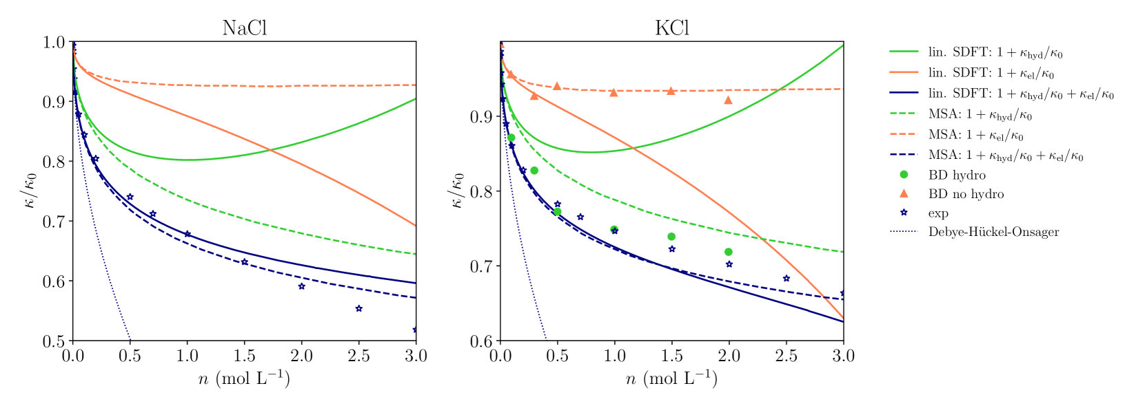
Figure 1: Comparison between linearized SDFT and MSA. Conductivity of NaCl (left) and KCl (right) electrolytes, rescaled by their value at infinite dilution $\kappa_{0}$, obtained from linearized SDFT (solid lines) and MSA (dashed lines). For KCl, we show results from Brownian dynamics simulations Jardat et al. (1999) (symbols), with and without hydrodynamics. The value of the conductivity is decomposed as the sum of its value at infinite dilution, an electrostatic contribution and a hydrodynamic contribution [Eq. (15)]. For both electrolytes, we also show results from experimental measurements of the conductivity (stars)Miller (1966). Finally, we represent the classical result from the Debye-Hückel-Onsager approachOnsager (1927) (dotted lines), which reads: $\frac{\kappa}{\kappa_{0}}=1-\left[\frac{\sqrt{2}}{3\sqrt{\pi}}\frac{\ell_{B}^{1/2}}{\eta\bar{\mu}}+\frac{2\sqrt{\pi}(\sqrt{2}-1)}{3}\ell_{B}^{3/2}\right]n^{1/2}$.

The electrostatic and hydrodynamic contributions are plotted on Fig. 1 for two simple monovalent electrolytes: NaCl and KCl. As noted in Ref. 27, the electrostatic and hydrodynamic contributions to conductivity diverge (to $-\infty$ and $+\infty$, respectively) when the concentration of the electrolyte is too high. In order to discuss the accuracy of the linearized SDFT approach, we compare the behaviors of these two contributions with earlier analytical results, that relied on the Mean Spherical Approximation (MSA).

electrolyte	$D_{0}^{+}$ ($10^{-9}\text{m}^{2}\cdot\text{s}^{-1}$)	$D_{0}^{-}$ ($10^{-9}\text{m}^{2}\cdot\text{s}^{-1}$)	$a$ (Å)	$r_{s}$ (Å)
LiCl	$1.03$	$2.03$	$2.57$	–
NaCl	$1.33$	$2.03$	$2.83$	$1.45$
KCl	$1.96$	$2.03$	$3.19$	–

Table 1: Summary of parameter values for the different electrolytes considered in the manuscript.

On Fig. 1, we plot the conductivity obtained from linearized SDFT [Eqs. (15)–(17), see Table 1 for the numerical parameters] and the conductivity obtained from MSA (the underlying assumptions and the derivation of the expressions of $\kappa_{\text{el}}$ and $\kappa_{\text{hyd}}$ are given in Section III). For both theories, we plot separately the different contributions, and several comments follow: (i) the main comment is that, although the total expression of the conductivity obtained from MSA and linearized SDFT appear to give very similar numerical values, the behavior of their hydrodynamic and electrostatic contributions are qualitatively and quantitatively different. In particular, the hydrodynamic contribution predicted by SDFT appear to be non-monotonic. This observation is not in agreement with Brownian dynamics simulations, which can be performed with and without hydrodynamic interactions, in order to decipher the role of the electrostatic and hydrodynamic contributions (simulation results obtained in the case of KCl electrolyte are also shown on Fig. 1). In addition, the electrostatic contribution is much more important in linearized SDFT than in MSA, but both effects seem to compensate; (ii) when compared to experimental measurements, the full expression obtained from linearized SDFT (blue solid lines) does not improve upon the MSA prediction (blue dashed lines). This observation prompted us to look for different ways to improve linearized SDFT in this context. In the next Section, we will see how the treatment of hydrodynamic interactions can be refined. At the end of the manuscript, we will discuss the role played by the details of the modified potential on the outcome of the linearized SDFT calculations.

V Accounting for the finite size of the ions in the hydrodynamic equations

The result for the hydrodynamic contribution to the conductivity, given in Eq. (17), is obtained by assuming that, from the point of view of hydrodynamics, the ions are point-like, so that their finite size only plays a role in the modified electrostatic potential. Indeed, denoting by $\delta\bm{u}$ and $\delta\rho=\delta n_{+}-\delta n_{-}$ the small perturbations around homogeneous states, the hydrodynamics equations read

$$\eta\nabla^{2}\delta\bm{u} =\nabla\delta p-e\delta\rho\bm{E}_{0},$$ (48)

$$\nabla\cdot\delta\bm{u} =0.$$ (49)

In the simplest possible description, their solutions are found assuming that the ions are pointlike, and neglecting possible boundary conditions at their surface. From a technical point of view, this is achieved by using the Oseen tensor, defined as

$$O_{ij}(\bm{r})=\frac{1}{8\pi\eta}\left(\frac{\delta_{ij}}{r}+\frac{r_{i}r_{j}}{r^{3}}\right),$$ (50)

which is the Green’s function to Eqs. (48) and (49) under these assumptions. The Fourier transform of this tensor reads

$$\tilde{O}_{ij}(\bm{k})=\frac{1}{\eta k^{2}}\left(\delta_{ij}-\frac{k_{i}k_{j}}{k^{2}}\right),$$ (51)

and the solution of Eqs. (48) and (49) isAvni et al. (2022):

$$\delta\tilde{\bm{u}} =e\tilde{\mathbf{O}}\cdot\bm{E}_{0}\delta\tilde{\rho}(\bm{k}),$$ (52)

$$=\frac{eE_{0}}{\eta k^{2}}\left(\delta_{ij}-\frac{k_{x}^{2}}{k^{2}}\right)\delta\tilde{\rho}(\bm{k}).$$ (53)

The expression of the hydrodynamic contribution to the conductivity, given in Eq. (17), follows from this expression.

This calculation can be improved by assuming that, from the point of view of hydrodynamics, the ions actually have a finite radius $r_{s}$ (the Stokes radius), and that the solvent has a no-slip boundary condition at the surface of the ions: $\bm{u}(r=r_{s})=0$. Under these assumptions, the Green’s function of Eqs. (48) and (49) is now the Rotne-Prager tensor, whose expression reads, in real spaceKim and Karrila (2005)

$$R_{ij}(\bm{r})= \frac{1}{6\pi\eta r_{s}}\left\{\frac{3}{4}\left(\frac{r_{s}}{r}\right)\left(\frac{\delta_{ij}}{r}+\frac{r_{i}r_{j}}{r^{3}}\right)\right.$$

$$\left.+\frac{1}{2}\left(\frac{r_{s}}{r}\right)^{3}\left({\delta_{ij}}-3\frac{r_{i}r_{j}}{r^{2}}\right)\right\}.$$ (54)

In principle, the anions and the cations have different hydrodynamic radii, so that the expression of the Rotne-Prager tensor would actually depend on the considered pair. However, we assume for simplicity that there is only one radius involved in the Rotne-Prager tensor, which is a reduced Stokes radius $r_{s}=1/(6\pi\eta\bar{\mu})$ (see Table 1 for numerical values). Note that this keeps the hydrodynamic description consistent with the modified potential given in Eq. (13), in which one assumes that the cutoff radius $a$ is the same for all the ion pairs. The Fourier transform of the Rotne-Prager tensor can be deduced quite easily from that of the Oseen tensor by noting that Kim and Karrila (2005):

$$\nabla^{2}\left(\frac{\delta_{ij}}{r}+\frac{r_{i}r_{j}}{r^{3}}\right)=2\left(\frac{\delta_{ij}}{r^{3}}-3\frac{r_{i}r_{j}}{r^{5}}\right),$$ (55)

which yields Beenakker (1986)

$$\tilde{R}_{ij}(\bm{k})=\frac{1}{\eta}\left(\delta_{ij}-\frac{k_{i}k_{j}}{k^{2}}\right)\left(\frac{1}{k^{2}}-\frac{r_{s}^{2}}{3}\right).$$ (56)

The expression of the perturbation to the velocity field induced by the displacement of the ions is now $\delta\tilde{\bm{u}}=e\tilde{\mathbf{R}}\cdot\bm{E}_{0}\delta\tilde{\rho}(\bm{k})$, and the result from $\kappa_{\text{hyd}}$ now reads:

$$\kappa_{\text{hyd}}= -\frac{2}{\pi}\frac{\kappa_{0}r_{s}}{\lambda_{D}}\int_{0}^{\frac{2\pi\lambda_{D}}{r_{s}}}\mathrm{d}x\left(1-\frac{r_{s}^{2}x^{2}}{3\lambda_{D}^{2}}\right)\frac{\cos\frac{ax}{\lambda_{D}}}{\cos\frac{ax}{\lambda_{D}}+x^{2}}.$$ (57)

Note that introducing the Rotne-Prager tensor makes the $x$-integral (i.e. the $k$-integral since we use the change of variable $x=k\lambda_{D}$) divergent at large $x$. This is regularized by introducing an upper cutoff which corresponds to the size of the ion. We show on Fig. 2 the linearized SDFT theory corrected by using the Rotne-Prager tensor instead of the Oseen tensor, for NaCl electrolyte. Interestingly, it seems like introducing this no-slip boundary condition for the solvent at $r=r_{s}$ regularizes the hydrodynamic contribution, or at least shifts its divergence to higher concentrations. At this point, it would be tempting to account for higher-order corrections in the treatment of the hydrodynamic interactions. Indeed, the multi-body hydrodynamic tensors, that allows one to go beyond the simple Rotne-Prager treatment and to account for multi-body hydrodynamic interactions, are known analytically Kim and Karrila (2005). However, this would be inconsistent with the treatment of the other interactions between the ions, which are only accounted for at the pair level in the usual DK framework [Eq. (1)].

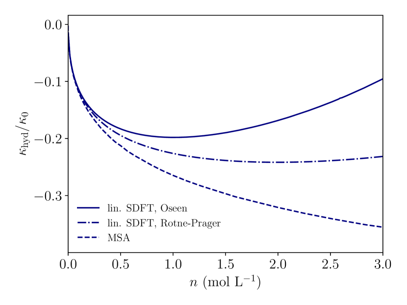
Figure 2: Hydrodynamic description at the Rotne-Prager level. Comparison of the different hydrodynamic contributions to the conductivity of NaCl electrolyte, rescaled by their value at infinite dilution $\kappa_{0}$, obtained from SDFT with the Rotne-Prager tensor (solid lines, Eq. (57)), linearized SDFT with the Oseen tensor (dash-dotted lines, Eq. (17)) and MSA (dashed lines, see Section III for details).

VI Self-diffusion coefficient

VI.1 General equations

We now turn to another observable, namely the self-diffusion coefficient of a tagged ion in the electrolyte. To compute this quantity, it is not necessary to assume that the electrolyte is submitted to a constant electric field force as in the calculation of the conductivity. Without loss of generality, our goal is to calculate the self-diffusion coefficient of the first cation and denote its position by $\bm{R}(t)\equiv\bm{r}_{1}^{+}(t)$. The positions of the ions are still assumed to obey the overdamped Langevin equations given by Eqs. (1)–(II.1) (with $\bm{E}_{0}=0)$. We now define the densities

$$n^{\prime}_{+}(\bm{r},t) =\sum_{a=2}^{N}\delta(\bm{r}-\bm{r}_{a}^{+}(t)),$$ (58)

$$n^{\prime}_{-}(\bm{r},t) =\sum_{a=1}^{N}\delta(\bm{r}-\bm{r}_{a}^{-}(t)).$$ (59)

Note that these quantities slightly differ from the densities defined earlier, as the contribution from the ion that plays the role of a tracer has been extracted from the summation. In what follows, we drop the ‘primes’ to ease the notation. The equation of motion for a cation (other than the tracer) then reads

$$\frac{\mathrm{d}}{\mathrm{d}t}\bm{r}^{+}_{a}(t)=\bm{u}(\bm{r}_{a}^{+}(t))+\sqrt{2D_{+}}\bm{\eta}_{a}^{+}(t)$$

$$-\mu_{+}\nabla\int\mathrm{d}\bm{r}^{\prime}\;V_{\text{co}}(\bm{r}_{a}^{+}(t)-\bm{r}^{\prime})[n_{+}-n_{-}+\delta(\bm{r}^{\prime}-\bm{R}(t))],$$ (60)

and that of an anion reads

$$\frac{\mathrm{d}}{\mathrm{d}t}\bm{r}^{-}_{a}(t)=\bm{u}(\bm{r}_{a}^{-}(t))+\sqrt{2D_{-}}\bm{\eta}_{a}^{-}(t)$$

$$-\mu_{-}\nabla\int\mathrm{d}\bm{r}^{\prime}\;V_{\text{co}}(\bm{r}_{a}^{-}(t)-\bm{r}^{\prime})[-n_{+}+n_{-}-\delta(\bm{r}^{\prime}-\bm{R}(t))],$$ (61)

where we denote by $V_{\text{co}}$ the modified Coulomb potential:

$$V_{\text{co}}(r)=\frac{e^{2}}{4\pi\varepsilon_{0}\varepsilon r}\theta(r-a).$$ (62)

We define $\rho=n_{+}-n_{-}$, and we summarize below the main equations that constitute the starting point of our calculation. The evolution equations for the densities $n_{+}$ and $n_{-}$ are obtained as before with Ito calculation Dean (1996)

$$\partial_{t}n_{\alpha}+\nabla\cdot\bm{j}_{\alpha}=0,$$ (63)

with the fluxes:

$$\bm{j}_{\alpha}=n_{\alpha}\bm{u}-D_{\alpha}\nabla n_{\alpha}-\sqrt{2D_{\alpha}n_{\alpha}}\bm{\zeta}_{\alpha}$$

$$-\mu_{\alpha}z_{\alpha}n_{\alpha}\int\mathrm{d}\bm{r}^{\prime}\;\nabla V_{\text{co}}(\bm{r}-\bm{r}^{\prime})[\rho(\bm{r}^{\prime},t)+\delta(\bm{r}^{\prime}-\bm{R}(t))],$$ (64)

where $z_{\pm}=\pm 1$, and where the noises $\bm{\zeta}_{\alpha}$ have zero average, and correlations given by Eq. (9). The equation of motion of the tracer particle reads

$$\frac{\mathrm{d}}{\mathrm{d}t}\bm{R}(t)=\bm{u}(\bm{R}(t))+\sqrt{2D_{+}}\bm{\eta}_{0}^{+}(t)$$

$$-\mu_{+}\nabla\int\mathrm{d}\bm{r}^{\prime}\;V_{\text{co}}(\bm{R}(t)-\bm{r}^{\prime})\rho(\bm{r}^{\prime},t),$$ (65)

with $\langle\bm{\eta}_{0}^{+}(t)\rangle=0$ and $\langle{\eta}_{0,i}^{+}(t){\eta}_{0,j}^{+}(t^{\prime})\rangle=\delta_{ij}\delta(t-t^{\prime})$. The velocity field of the solvent, denoted by $\bm{u}$, obeys the following hydrodynamic equations (Stokes equation and incompressibility condition):

$$\nabla\cdot\bm{u}=0$$ (66)

$$\eta\nabla^{2}\bm{u}=\nabla p-\delta(\bm{r}-\bm{R}(t))\int\mathrm{d}\bm{r}^{\prime}\nabla V_{\text{co}}(\bm{r}-\bm{r}^{\prime})\rho(\bm{r}^{\prime},t)$$

$$-\rho(\bm{r},t)\int\mathrm{d}\bm{r}^{\prime}\;\nabla V_{\text{co}}(\bm{r}-\bm{r}^{\prime})[\rho(\bm{r}^{\prime},t)+\delta(\bm{r}^{\prime}-\bm{R}(t))]$$ (67)

where $p$ is the pressure field in the solvent.

These equations are then linearized using the perturbative expansions:

$$n_{\pm} =n+\delta n_{\pm},$$ (68)

$$\rho =n_{+}-n_{-}=\delta n_{+}-\delta n_{-},$$ (69)

$$\bm{u} =\delta\bm{u},$$ (70)

$$p =p_{0}+\delta p.$$ (71)

Note that, although the densities $n_{+}$ and $n_{-}$ do not correspond to the exact same number of ions ($N-1$ for the cation density and $N$ for the anion density), we still linearize them around the same constant value $n=N/V$, which is a valid approximation in the thermodynamic limit ($N\to\infty$ and $V\to\infty$ with fixed number density $n=N/V$). At leading order in these perturbations, we get the following evolution equations for the densities $\delta n_{+}$ and $\delta n_{-}$ in Fourier space

$$\partial_{t}\delta\tilde{n}_{\alpha}=-D_{\alpha}k^{2}\delta\tilde{n}_{\alpha}+\sqrt{2D_{\alpha}n}\bm{k}\cdot\tilde{\bm{\zeta}}_{\alpha}(\bm{k})$$

$$-\mu_{\alpha}nz_{\alpha}k^{2}\tilde{V}_{\text{co}}(\bm{k})\tilde{\rho}-\mu_{\alpha}nz_{\alpha}k^{2}\tilde{V}_{\text{co}}(\bm{k})\mathrm{e}^{-\mathrm{i}\bm{k}\cdot\bm{R}(t)}.$$ (72)

Interestingly, we observe that the velocity field does not appear anymore in the equations for the density fields $\delta\tilde{c}_{\alpha}$. This is due to the incompressibility condition:

$$\nabla\cdot(n_{\alpha}\bm{u})=\nabla\cdot[(n+\delta n_{\alpha})\delta\bm{u}]\simeq n\nabla\cdot\delta\bm{u}=0$$ (73)

The hydrodynamic equations now read:

$$\nabla\cdot\bm{u} =0$$ (74)

$$\eta k^{2}\delta\tilde{\bm{u}} =-\mathrm{i}\bm{k}\delta\tilde{p}$$ (75)

At leading order, the forces exerted by the ions on the solvent vanish, and the effect of solvent flows on the dynamics of the ions is then negligible. Indeed, the interaction terms in the Stokes equation vanish because they either involve contributions of order $\delta\rho^{2}$ or terms of order $\delta\rho\times\delta_{\bm{R}(t)}$, which are negligible since $|\delta_{\bm{R}(t)}|\sim 1/V$ where $V$ is the volume of the system. Therefore, the choice of the right description for boundary conditions at the surface of the ions, that was discussed in Section V, is here irrelevant .

We finally end up with the set of equations (with $\alpha=\pm 1$):

$$\frac{\mathrm{d}}{\mathrm{d}t}\bm{R}(t)=+\sqrt{2D_{+}}\bm{\eta}_{0}^{+}(t)$$

$$-\mu_{+}\nabla\int\mathrm{d}\bm{r}^{\prime}V_{\text{co}}(\bm{R}(t)-\bm{r}^{\prime})[\delta n_{+}(\bm{r}^{\prime},t)-\delta n_{-}(\bm{r}^{\prime},t)],$$ (76)

$$\partial_{t}\delta\tilde{n}_{\alpha}=-D_{\alpha}k^{2}\delta\tilde{n}_{\alpha}+\sqrt{2D_{\alpha}n}\bm{k}\cdot\tilde{\bm{\zeta}}_{\alpha}(\bm{k})$$

$$-\mu_{\alpha}nz_{\alpha}k^{2}\tilde{V}_{\text{co}}(\bm{k})(\delta\tilde{n}_{+}-\delta\tilde{n}_{-})-\mu_{\alpha}nz_{\alpha}k^{2}\tilde{V}_{\text{co}}(\bm{k})\mathrm{e}^{-\mathrm{i}\bm{k}\cdot\bm{R}(t)},$$ (77)

that fully determine the dynamics of the tagged ion and that of the ionic density fields within the linearized approximation. The counterpart of these equations when the tracer is an anion can be obtained straightforwardly.

VI.2 Path-integral formulation

The first equation [Eq. (76)] can be seen as a simple Langevin equation that describes the motion of the tracer particle. However, it is not easy to compute the associated effective diffusion coefficient. Indeed, this equation of motion involves on its rhs a functional of the density fields $\delta n_{\alpha}$, whose evolution equations [Eq. (77)] also depends on the tracer position $\bm{R}(t)$. We then end up with a set of equations which are coupled nonlinearly.

A way to treat this coupling was proposed by Dean and Démery Démery and Dean (2011), who proposed a perturbative path-integral method, to compute the effective diffusion coefficient of the tracer at leading order in the coupling between the tracer and a fluctuating environment. Here, the situation is more complicated, because the tracer interacts with two fields at the same time (the density field of cations and that of anions). We recently extended the Dean-Démery method to compute perturbatively the diffusion coefficient of a tracer coupled to multiple fields Jardat, Dahirel, and Illien (2022).

We apply this method to the present case and obtain the following expression for the diffusion coefficient of the tagged cation rescaled by its bare value $D_{+}$ (the formula below applies to both situations where the tracer is a cation or an anion):

$$\frac{D_{\text{eff},+}}{D_{+}}=1-\sum_{\alpha,\beta=\pm}\frac{\overline{D}_{\alpha\beta}}{D_{+}}$$ (78)

with

$$\frac{\overline{D}_{\alpha\beta}}{D_{+}}=\frac{\mu_{+}\mu_{\beta}}{d}\int\frac{\mathrm{d}^{d}\bm{k}}{(2\pi)^{d}}k^{4}nz_{\alpha}\tilde{V}_{\text{co}}^{2}\sum_{\gamma}z_{\gamma}$$

$$\times\sum_{\nu=\pm 1}\frac{2c_{\alpha\beta}^{(\nu)}}{(D_{+}k^{2}+\Lambda_{\nu})^{2}}\left[\delta_{\gamma\beta}+(D_{+}k^{2}-\Lambda_{\nu})\sum_{\epsilon=\pm 1}\frac{c_{\gamma\beta}^{(\epsilon)}}{\Lambda_{\nu}+\Lambda_{\epsilon}}\right]$$ (79)

where we defined the matrices,

$$\bm{m} =k^{2}\begin{pmatrix}\mu_{+}(k_{\mathrm{B}}T+n\tilde{V}_{\text{co}})&-\mu_{+}n\tilde{V}_{\text{co}}\\ -\mu_{-}n\tilde{V}_{\text{co}}&\mu_{-}(k_{\mathrm{B}}T+n\tilde{V}_{\text{co}})\end{pmatrix},$$ (80)

$$\bm{c^{(\pm)}} =\frac{1}{2s}\begin{pmatrix}{\pm m_{++}\mp m_{--}+s}&\pm 2{m_{+-}}\\ \pm 2{m_{-+}}&\mp m_{++}\pm m_{--}+s\end{pmatrix},$$ (81)

the eigenvalues

$$\Lambda_{\pm}=\frac{m_{++}+m_{--}}{2}\pm\frac{1}{2}\sqrt{(m_{++}-m_{--})^{2}+4m_{+-}m_{-+}},$$ (82)

and the quantity

$$s=\sqrt{(m_{++}-m_{--})^{2}+4m_{+-}m_{-+}}.$$ (83)

In order to get a more compact expression of the diffusion coefficient, it is convenient to introduce a dimensionless interaction potential $\tilde{U}(k)=n\tilde{V}_{\mathrm{co}}(k)/k_{\mathrm{B}}T$. Relying on the fact that the integrand in the $\bm{k}$-integral from Eq. (VI.2) is spherically symmetric to perform the angular integration, specifying this expression to the case $d=3$, we get the following formula, which applies to both situations where the tracer is a cation or an anion ($D_{0}$ denotes the corresponding bare diffusion coefficient):

$$\frac{D_{\text{eff}}}{D_{0}}=1-\int_{0}^{\infty}\mathrm{d}k\frac{32k^{2}}{\pi^{2}n}(3+\Delta)(3\Delta\tilde{U}+2\Delta+\tilde{U}+2)\Delta\tilde{U}^{2}$$

$$\times[((\tilde{U}+3)+(\tilde{U}+1)\Delta)^{2}-S^{2}]^{-2}[((\tilde{U}+1)^{2}(\Delta+1)^{2}-S^{2}]^{-1}$$

where we introduced the shorthand notation

$$S=\sqrt{(\Delta+1)^{2}\tilde{U}^{2}+(\Delta-1)^{2}(2\tilde{U}+1)},$$ (85)

and where $\Delta=D_{0}^{-}/D_{0}^{+}$ (resp. $D_{0}^{+}/D_{0}^{-}$) if the tracer is a cation (resp. an anion). Eq. (LABEL:Deff_full_exp) provides an explicit and general expression for the effective diffusion coefficient of a tagged ion in the electrolyte, and it is the main result of this Section. Although the $k$-integral can be divergent depending on the analytical expression of the interaction potential Démery and Dean (2011); Jardat, Dahirel, and Illien (2022), we will focus on the truncated potential given in Eq. (13), which does not cause any small-$k$ or large-$k$ divergence, and which yields the following rescaled potential $\tilde{u}$:

$$\tilde{U}(k)=4\pi n\ell_{B}\frac{\cos(ka)}{k^{2}}.$$ (86)

Consequently, the general expression given in Eq. (LABEL:Deff_full_exp) only depends on three parameters: the electrolyte concentration $n$, the cutoff of the truncated potential $a$ (which will typically be measured in units of the Bjerrum length, setting the dimensionless parameter $\bar{a}=a/\ell_{B}$), and the ratio between the bare diffusion coefficient $\Delta$. We now consider a few limit cases of Eq. (LABEL:Deff_full_exp).

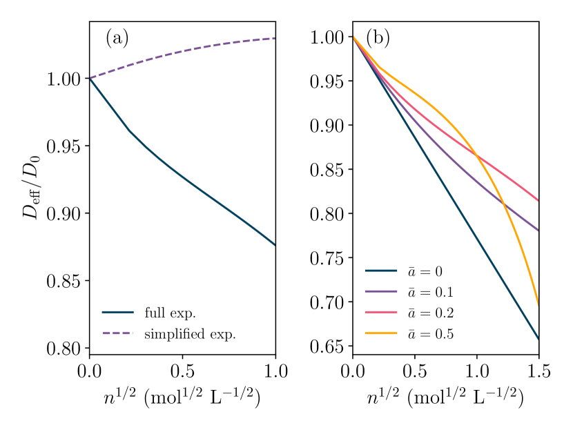
Figure 3: Self-diffusion: case where cations and anions have the same mobility. (a) Self-diffusion coefficient as a function of the square-root concentration $n^{1/2}$ as obtained from the ‘full expression’ [Eq. (VI.3)] and the ‘simplified expression’ [Eq. (VI.3)]: the latter is obtained by neglecting the effect of the tracer on the bath. In both cases, we take $\bar{a}=a/\ell_{B}=0.3$. (b) Self-diffusion coefficient as a function of the square-root concentration $n^{1/2}$ as given by Eq. (VI.3), for several values of the rescaled cutoff value $\bar{a}$. For $\bar{a}=0$, we used the expression Eq. (89).

VI.3 Case where anions and cations have the same mobility

We first focus on the particular case (which applies to KCl) where anions and cations have the same mobility. In this situation, we get the following expression for the effective diffusion coefficient of the tracer, which is very simple and explicit:

$$\frac{D_{\text{eff}}}{D_{0}}=1-\int_{0}^{\infty}\mathrm{d}k\frac{8k^{2}}{3}{n\ell_{B}^{2}\cos^{2}(ka)}$$

$$\times\Big{\{}[4\pi\cos(ka)\ell_{B}n+k^{2}][8\pi\cos(ka)\ell_{B}n+k^{2}]\Big{\}}^{-1}.$$ (87)

This expression is plotted on Fig. 3(a): as expected, the self-diffusion coefficient of an ion in the electrolyte is a decreasing function of the concentration.

A frequent simplification of the derivation presented in Section VI.2 consists in neglecting the effect of the tracer on the dynamics of the density fields. This is referred to as the ‘passive case’ in Ref. 65), and has been used in different contextsDean, Drummond, and Horgan (2007); Leitenberger, Reister-Gottfried, and Seifert (2008); Marbach, Dean, and Bocquet (2018); Wang et al. (2023). Concretely, this is equivalent to neglecting the last term in the rhs of Eq. (77). This yields the following expression for the effective diffusion coefficient of the tracer:

$$\frac{D_{\text{eff}}}{D_{0}}=1+\int_{0}^{\infty}\mathrm{d}k\frac{32\pi k^{2}}{3}{n^{2}\ell_{B}^{3}\cos^{3}(ka)}$$

$$\times\Big{\{}[4\pi\cos(ka)\ell_{B}n+k^{2}]^{2}[8\pi\cos(ka)\ell_{B}n+k^{2}]\Big{\}}^{-1}$$ (88)

It is interesting to note that this simplified version actually predicts an unphysical behavior for the diffusion coefficient, which becomes an increasing function of the overall concentration, and therefore exceeds its bare value as concentration increases (Fig. 3(a)). This observation indicates that this simplification should be used with caution.

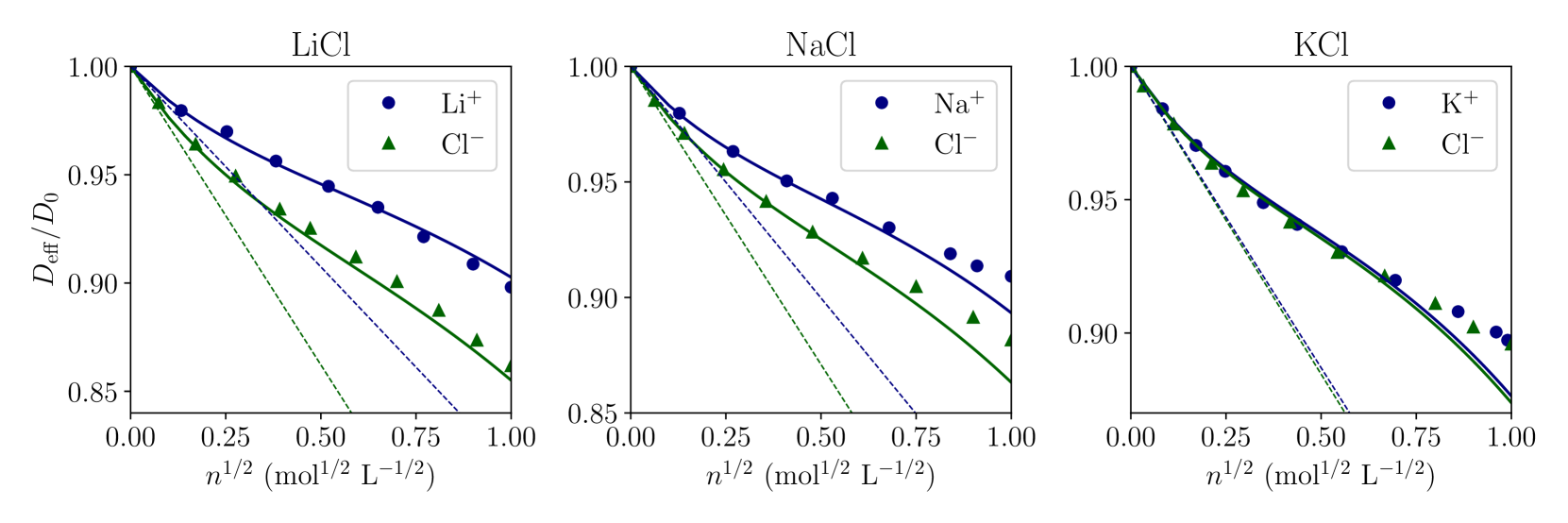
Figure 4: Self-diffusion coefficients of ions in the electrolytes LiCl, NaCl and KCl: results obtained from linearized SDFT (Eq. (LABEL:Deff_full_exp), solid lines) and from the MCT/MSA calculation (Ref. 7, symbols). Dashed lines: Onsager limiting law [Eq. (89)].

VI.4 Case of a vanishing interaction radius ($a\to 0$)

We now consider the limit of vanishing interaction radius ($a\to 0$) in Eq. (LABEL:Deff_full_exp). In this situation, the integral over $k$ can be computed exactly, and yields:

$$\lim_{a\to 0}\frac{D_{\text{eff}}}{D_{0}}=1-\frac{2\sqrt{\pi}}{3}\left(\sqrt{2}-\sqrt{\frac{1+3\Delta}{2(1+\Delta)}}\right)\sqrt{n\ell_{B}^{3}}.$$ (89)

Interestingly, this coincides exactly with the limiting law predicted by Onsager Onsager (1945); Onsager and Fuoss (1932).

In order to investigate the accuracy of this simplified expression, we compare it to results obtained from Eq. (LABEL:Deff_full_exp) with a fixed value of $\Delta$ and several values of the rescaled cutoff value $\bar{a}=a/\ell_{B}$ (Fig. 3(b)). Although the truncated potential is very simplified, we observe that introducing a cutoff value $a$ below which the potential vanishes has a significant impact on the self-diffusion coefficient of the tracer. A similar conclusion was reached when comparing the conductivity predicted by the Debye-Hückel-Onsager theory with the results from SDFT Avni et al. (2022).

VI.5 General case and comparison to mode coupling theory/MSA

We finally confront the result we obtained from linearized SDFT [Eq. (LABEL:Deff_full_exp)] with earlier results obtained from a combination of mode-coupling theory (MCT) and the mean spherical approximation (MSA) Dufrêche et al. (2002, 2005) . We consider three electrolytes: LiCl, NaCl and KCl. As input to our analytical theory, we use the values of the bare diffusion coefficients given in Ref. 10 and the values of the cutoff distances for the modified Coulomb potential given in Ref. 26. These values are recalled in Table 1. Results are shown on Fig. 4. We find that, for these three electrolytes, the self-diffusion coefficients estimated from linearized SDFT calculations are very close to the MSA results. We may attribute this to the fact that the hydrodynamic contributions, that appear to be wrongly estimated by linearized SDFT (at least when it comes to the conductivity, see Section V) do not have any effect on the self-diffusion coefficient at this order of approximation. A similar property held within the MSA/MCT treatment mentioned above.

VII Importance of the choice of the modified potential

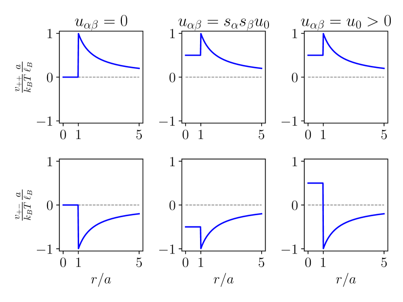
Figure 5: Modified interaction potentials: as defined in Eq. (90), for different choices of the parameter $u_{\alpha\beta}$. The last case, where $u_{\alpha\beta}=u_{0}$ for all pairs $(\alpha,\beta)$, is discussed in Appendix B.

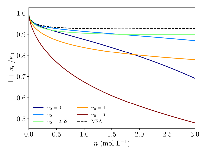
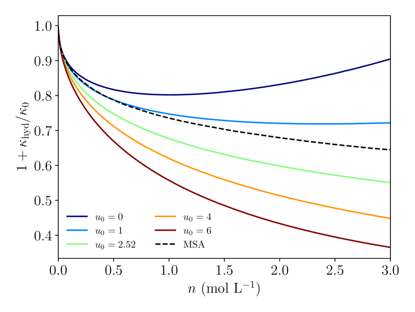
Figure 6: Influence of the repulsion parameter on the conductivity. Electrostatic (left) and hydrodynamic (right) contributions to conductivity, with the modified Coulomb potential given in Eq. (90), and the repulsive contribution from Eq. (91), for different values of the repulsion parameter $u_{0}$ (solid lines). The value $u_{0}=2.52$ corresponds to $u_{0}=a/\ell_{B}$. Dashed lines: results from MSA calculations [Eqs. (44) and (28)].

So far, we considered the modified Coulomb potential given in Eq. (13), which is obtained by truncating the Coulomb interaction below a radius $r=a$ and setting the interaction energy to 0 below this cutoff. In this Section, we will show how the modifications of this potential, by changing the nature of the short-range part, can affect the observables we have considered so far, namely conductivity and self-diffusion. For this purpose, we rewrite the potential $v_{\alpha\beta}(r)$ under the form:

$$v_{\alpha\beta}(r)=z_{\alpha}z_{\beta}V_{\text{co}}(r)+u_{\alpha\beta}\theta(a-r).$$ (90)

The first term corresponds to the truncated potential studied so far, the second term is a step ‘repulsion’ term, written as a simple rectangular function whose magnitude can be controlled with the parameter $u_{\alpha\beta}$ ($u_{\alpha\beta}=0$ corresponds to the case studied so far, and is represented on Fig. 5). In what follows, we study different possible choices for this parameter.

VII.1 Conductivity

A first option consists in assuming that the repulsion parameter $u_{\alpha\beta}$ depends on the considered pair. More precisely, we make the choice:

$$u_{\alpha\beta}=z_{\alpha}z_{\beta}u_{0},$$ (91)

in such a way that $u_{\alpha\beta}=u_{0}$ (resp. $-u_{0}$) if both ions have the same charge (resp. opposite charges). Although this is not the most physical choice (short-range repulsion is usually modeled by a charge-independent contribution), this choice is motivated by the fact that it can be used to make the interaction potential $v_{\alpha\beta}$ continuous at the cutoff value $r=a$, with the choice $u_{0}=\ell_{B}/a$. The case where the short-range contribution is charge-independent ($u_{\alpha\beta}=u_{0}$) is discussed in Appendix B.

The Fourier transform of the modified potential now reads

$$\tilde{v}_{\alpha\beta}(k)=\frac{k_{\mathrm{B}}T}{2n\lambda_{D}^{2}k^{2}}\left[\cos ka+\frac{u_{0}}{\ell_{B}k}(\sin ka-ka\cos ka)\right].$$ (92)

It is straightforward to show that the corresponding expressions of $\kappa_{\text{el}}$ and $\kappa_{\text{hyd}}$ are obtained from Eqs. (16) and Eqs. (17) by making the substitution:

$$\cos\frac{ax}{\lambda_{D}}\to\cos\frac{ax}{\lambda_{D}}+\frac{\lambda_{D}u_{0}}{x\ell_{B}}\left(\sin\frac{ax}{\lambda_{D}}-\frac{ax}{\lambda_{D}}\cos\frac{ax}{\lambda_{D}}\right)$$ (93)

Importantly, the integrals involved in the expressions of $\kappa_{\text{el}}$ and $\kappa_{\text{hyd}}$ diverge in the limit $u_{0}\to\infty$, which is consistent with the general idea that linearized SDFT cannot account for hardcore interactions. We show on Fig. 6 the influence of the value of $u_{0}$ on the electrostatic contribution to the conductivity. Starting from $u_{0}=0$, which corresponds to the previous situation, and increasing $u_{0}$ up to the value $(\ell_{B}/a)k_{\mathrm{B}}T$, where the modified potential becomes continuous at $r=a$, we observe that the electrostatic contribution gets closer and closer to the value predicted by MSA. When $u_{0}\gg k_{\mathrm{B}}T$, the magnitude of the electrostatic contribution tends to diverge, as can be predicted from its analytical expression. Therefore, it seems that there exists an optimal value for the parameter $u_{0}$, that significantly improves the estimates from linearized SDFT when compared to earlier analytical schemes. A similar observation can be made about the hydrodynamic contribution, which appears to be closer to predictions from MSA calculations when $u_{0}$ is in the range $1-2~{}k_{\mathrm{B}}T$ (Fig. 6).

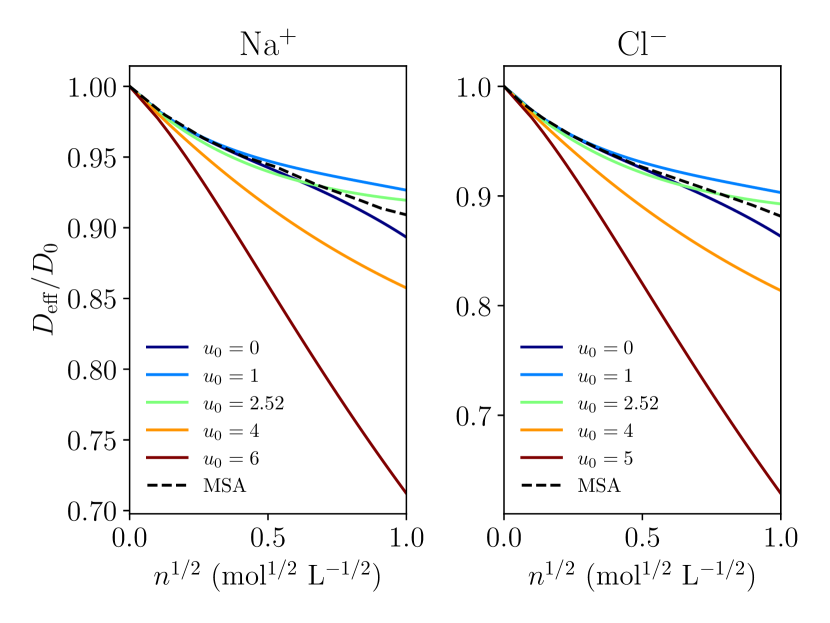
Figure 7: Influence of the repulsion parameter on self-diffusion. Self-diffusion coefficients of ions in NaCl electrolyte, with the modified Coulomb potential given in Eq. (90), and the repulsive contribution from Eq. (91), for different values of the repulsion parameter $u_{0}$ (solid lines). The value $u_{0}=2.52$ corresponds to $u_{0}=a/\ell_{B}$. Dashed lines: results from MSA/MCT calculations.

VII.2 Self-diffusion

The effect of the value of the repulsion parameter on self-diffusion can be studied in a similar way, by modifying the results obtained in Section VI. Technically, in Eq. (LABEL:Deff_full_exp), we replace the potential $\tilde{u}$ by the expression given in Eq. (92). We observe that, just like the conductivity, the self-diffusion coefficient is highly sensitive to the value of the repulsion parameter, and that its choice significantly affect the quality of the predictions from linearized SDFT when compared to results from the MCT-MSA framework (Fig. 7).

VIII Conclusion

In this work, we discussed several analytical theories for the conductivity and self-diffusion in concentrated electrolytes. Among them, linearized SDFT has been used quite extensively during the past years, and it allowed very successful predictions in the limit where electrolytes are very dilute. Recently, this analytical method was extended to study concentrated electrolytes, in which the short-range repulsion between ions plays a predominant role. A small-distance truncation of the Coulomb potential, which is tractable within linearized SDFT, has been put forward in order to account for short-range effects in a very simple fashion.

We showed that, within this approximation, the output of linearized SDFT contradicts earlier analytical (Mean-Spherical Approximation) and numerical (Brownian dynamics) estimates of the conductivity of concentrated electrolytes. However, the linearized SDFT treatment can be improved in several ways: (i) the hydrodynamic effects can be accounted at the Rotne-Prager level rather than at the Oseen tensor, which regularizes the hydrodynamic contribution to conductivity, or which at least shifts any unphysical divergence to higher densities; (ii) the short-range interaction energy between ions, which was set to zero in earlier treatments, can instead be set to a finite value, which may indeed improve the validity of the results by Avni et al.Avni et al. (2022) when compared to other analytical schemes such as MSA. Finally, we also computed the self-diffusion coefficient of ions within SDFT: as opposed to the conductivity, it appears that the dependence of this observable over ionic concentrations can be captured more easily by the truncated interaction, but that it is still highly dependent on the short-range details of the potential.

In conclusion, linearized SDFT is a particularly appealing tool to compute transport and diffusion properties in fluctuating systems of interacting particles, given its relative simplicity and ability to yield explicit expressions. However, we emphasize that, in spite of its advantages, it should be handled with caution, in particular when it comes to describing effects dominated by the short-range interactions between particles. Earlier analytical schemes, which often treat these interactions in a more thorough manner, should be used as a guide for the approximations that are implemented within linearized SDFT. Finally, we emphasize that computational approaches that rely on an implicit or coarse-grained representation of the solvent, and which often correspond to the same level of description than SDFT, constitute a very fertile field of researchLadiges et al. (2022); Kuron et al. (2016); Tischler et al. (2022), that usefully complement analytical descriptions.

Appendix A Direct correlation functions under the Mean Spherical Approximation

In this Appendix, we recall the expression of the direct correlation functions that can be derived under the Mean Spherical Approximation (see Section III.1 for details and references). These functions can be written under the form:

$$\tilde{c}_{\alpha\beta}(k)=-\frac{4\pi z_{\alpha}z_{\beta}\ell_{B}}{k^{2}}+{\tilde{c}}^{s}_{\alpha\beta}(k).$$ (94)

While the random phase approximation consists in assuming ${\tilde{c}}^{s}_{\alpha\beta}(k)=0$, the mean spherical approximation yields:

$${\tilde{c}}^{s}_{\alpha\beta}(k)= \frac{4\pi a^{3}}{K^{6}}[24d_{\alpha\beta}-2b_{\alpha\beta}K^{2}+e_{\alpha\beta}K^{4}$$

$$-[24d_{\alpha\beta}-2(b_{\alpha\beta}+6d_{\alpha\beta})K^{2}$$

$$+(a_{\alpha\beta}+b_{\alpha\beta}+d_{\alpha\beta}+e_{\alpha\beta})K^{4}]\cos K$$

$$+[-24d_{\alpha\beta}K+(a_{\alpha\beta}+2b_{\alpha\beta}+4d_{\alpha\beta})K^{3}]\sin K],$$ (95)

where we use the shorthand notation $K=ka$ for the dimensionless wavevector, and where we define:

$$a_{\alpha\beta} =-\frac{(1+2\eta)^{2}}{(1-\eta)^{4}}-2B\left(\frac{a}{\lambda_{D}}\right)\frac{\ell_{B}}{a}z_{\alpha}z_{\beta},$$ (96)

$$b_{\alpha\beta} =-\frac{6\eta(1+\eta/2)^{2}}{(1-\eta)^{4}}+\left[B\left(\frac{a}{\lambda_{D}}\right)\right]^{2}\frac{\ell_{B}}{a}z_{\alpha}z_{\beta},$$ (97)

$$d_{\alpha\beta} =-\frac{\eta(1+2\eta)^{2}}{2(1-\eta)^{4}},$$ (98)

$$e_{\alpha\beta} =\frac{\ell_{B}}{a}z_{\alpha}z_{\beta},$$ (99)

$$B(x) =\frac{x^{2}+x-x\sqrt{1+2x}}{x^{2}},$$ (100)

with $\eta=\frac{\pi}{6}a^{3}(n_{+}+n_{-})$ the total packing fraction.

Appendix B Alternative modification of the Coulomb potential

In this Appendix, we consider an alternative modification of the Coulomb potential, and assume that the repulsive part does not depend on the charge of the ion ($u_{\alpha\beta}=u_{0}$ for all pairs $\alpha$, $\beta$). We actually consider the following general expression for the pair potential:

$$v_{\alpha\beta}(r)=z_{\alpha}z_{\beta}\frac{e^{2}}{4\pi\varepsilon_{0}\varepsilon r}\theta(r-a)+v_{\text{rep}}(r),$$ (101)

where the repulsive part can first remained unspecified. With this choice, the symmetry relation $V_{++}=-V_{+-}$ does not hold anymore. Consequently, the field-field correlations (which are found as the solutions of the linearized DK equations for the cation and anion density fields) have different symmetries than in the situations considered before. First, we find that, under these conditions, the repulsive part of the potential $v_{\text{rep}}$ has no influence on the hydrodynamic contribution. Therefore it is sill given by Eq. (17).

Second, we find the following expression for the electrostatic contribution:

$$\kappa_{\text{el}}=-2e\bar{\mu}\int\frac{\mathrm{d}\bm{k}}{(2\pi)^{3}}{n^{2}k_{z}^{2}(\tilde{v}_{\text{co}}(k)-\tilde{v}_{\text{rep}}(k))^{2}}$$

$$\times\left[4k^{2}(\frac{1}{2}+n\tilde{v}_{\text{co}}(k))(\frac{1}{2}+n\tilde{v}_{\text{rep}})[1+n(\tilde{v}_{\text{co}}+\tilde{v}_{\text{rep}})]\right]^{-1}$$ (102)

where we introduced $\tilde{v}_{\text{co}}(k)=\tilde{V}_{\text{co}}(k)/k_{\mathrm{B}}T$ and $\tilde{v}_{\text{rep}}(k)=\tilde{V}_{\text{rep}}(k)/k_{\mathrm{B}}T$. In order to get a more explicit expression, we write the repulsive part as before, under the form $V_{\text{rep}}(r)=k_{\mathrm{B}}Tu_{0}\theta(a-r)$. We get the following expression for the electrostatic contribution:

$$\kappa_{\text{el}}=-\frac{1}{3\pi}\frac{\kappa_{0}\ell_{B}}{\lambda_{D}}\int_{0}^{\infty}\mathrm{d}x\frac{x^{2}\left(\cos\frac{ax}{\lambda_{D}}-\frac{u_{0}\lambda_{D}}{\ell_{B}x}\varphi\left(\frac{ax}{\lambda_{D}}\right)\right)^{2}}{\left(x^{2}+\cos\frac{ax}{\lambda_{D}}\right)\left(1+\frac{u_{0}\lambda_{D}}{\ell_{B}x^{3}}\varphi\left(\frac{ax}{\lambda_{D}}\right)\right)\left(x^{2}+\frac{1}{2}\cos\frac{ax}{\lambda_{D}}+\frac{u_{0}\lambda_{D}}{2\ell_{B}x}\varphi\left(\frac{ax}{\lambda_{D}}\right)\right)},$$ (103)

where we introduced the shorthand notation $\varphi(X)=\sin X-X\cos X$. We show on Fig. 8 the electrostatic contribution to conductivity as a function of the electrolyte concentration, for different values of the parameters $u_{0}$. As opposed to the case considered in Section VII, it is difficult to improve the predictions from linearized SDFT with this choice of the repulsive contribution.

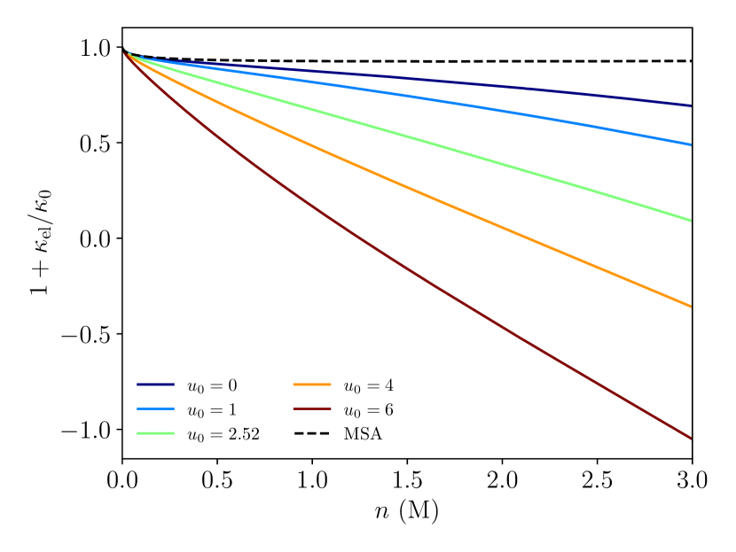
Figure 8: Influence of the repulsion parameter on the conductivity. Electrostatic contribution to conductivity, with the modified Coulomb potential given in Eq. (101) for different values of the repulsion parameter $u_{0}$ (solid lines). The value $u_{0}=2.52$ corresponds to $u_{0}=a/\ell_{B}$. Dashed line: results from MSA [Eq. (44)].

References

- Onsager (1927) L. Onsager, “Report on a revision of the conductivity theory,” Trans. Faraday Soc. 23, 341–349 (1927).
- Falkenhagen and Ebeling (1965) H. Falkenhagen and W. Ebeling, “Statistical derivation of diffusion equations according to the Zwanzig method,” Phys. Lett. 15, 131 (1965).
- Falkenhagen, Ebeling, and Kraeft (1971) H. Falkenhagen, W. Ebeling, and W. D. Kraeft, “Mass Transport Properties of Ionized Dilute Electrolytes,” in Ionic Interactions, Vol. 1, edited by S. Petrucci (Academic Press, New York, 1971) Chap. 2.
- Bernard et al. (1992a) O. Bernard, W. Kunz, P. Turq, and L. Blum, “Conductance in electrolyte solutions using the mean spherical approximation,” Journal of Physical Chemistry 96, 3833–3840 (1992a).
- Bernard et al. (1992b) O. Bernard, W. Kunz, P. Turq, and L. Blum, “Self-Diffusion in Electrolyte Solutions Using the Mean Spherical Approximation,” J. Phys. Chem. 96, 398–403 (1992b).
- Chhih et al. (1994) A. Chhih, P. Turq, O. Bernard, J. M. G. Barthel, and L. Blum, “Transport coefficients and apparent charges of concentrated electrolyte solutions - Equations for practical use,” Berichte der Bunsengesellschaft für physikalische Chemie 98, 1516–1525 (1994).
- Dufrêche et al. (2005) J. F. Dufrêche, O. Bernard, S. Durand-Vidal, and P. Turq, “Analytical theories of transport in concentrated electrolyte solutions from the MSA,” Journal of Physical Chemistry B 109, 9873–9884 (2005).
- Chandra and Bagchi (1999) A. Chandra and B. Bagchi, “Ion conductance in electrolyte solutions,” Journal of Chemical Physics 110, 10024–10034 (1999).
- Chandra and Bagchi (2000) A. Chandra and B. Bagchi, “Beyond the classical transport laws of electrochemistry: New microscopic approach to ionic conductance and viscosity,” Journal of Physical Chemistry B 104, 9067–9080 (2000).
- Dufrêche et al. (2002) J. F. Dufrêche, O. Bernard, P. Turq, A. Mukherjee, and B. Bagchi, “Ionic self-diffusion in concentrated aqueous electrolyte solutions,” Phys. Rev. Lett. 88, 095902 (2002).
- Contreras Aburto and Nägele (2013) C. Contreras Aburto and G. Nägele, “A unifying mode-coupling theory for transport properties of electrolyte solutions. I. General scheme and limiting laws,” Journal of Chemical Physics 139, 134109 (2013).
- Aburto and Nägele (2013) C. C. Aburto and G. Nägele, “A unifying mode-coupling theory for transport properties of electrolyte solutions. II. Results for equal-sized ions electrolytes,” Journal of Chemical Physics 139, 134110 (2013).
- Turq, Lantelme, and Friedman (1977) P. Turq, F. Lantelme, and H. L. Friedman, “Brownian dynamics: Its application to ionic solutions,” The Journal of Chemical Physics 66, 3039–3044 (1977).
- Trullàs, Giró, and Padró (1990) J. Trullàs, A. Giró, and J. A. Padró, “Langevin dynamics study of NaCl electrolyte solutions at different concentrations,” The Journal of Chemical Physics 93, 5177–5181 (1990).
- Kunz, Calmettes, and Turq (1990) W. Kunz, P. Calmettes, and P. Turq, “Structure of nonaqueous electrolyte solutions by small-angle neutron scattering, hypernetted chain, and Brownian dynamics,” The Journal of Chemical Physics 92, 2367–2373 (1990).
- Canales and Sesé (1998) M. Canales and G. Sesé, “Generalized Langevin dynamics simulations of NaCl electrolyte solutions,” Journal of Chemical Physics 109, 6004–6011 (1998).
- Jardat et al. (1999) M. Jardat, O. Bernard, P. Turq, and G. R. Kneller, “Transport coefficients of electrolyte solutions from Smart Brownian dynamics simulations,” Journal of Chemical Physics 110, 7993–7999 (1999).
- Batôt et al. (2013) G. Batôt, V. Dahirel, G. Mériguet, A. A. Louis, and M. Jardat, “Dynamics of solutes with hydrodynamic interactions : Comparison between Brownian dynamics and stochastic rotation dynamics simulations,” Phys. Rev. E 88, 043304 (2013).
- Dahirel, Bernard, and Jardat (2020) V. Dahirel, O. Bernard, and M. Jardat, “Can we describe charged nanoparticles with electrolyte theories? Insight from mesoscopic simulation techniques,” Journal of Molecular Liquids 303, 111942 (2020).
- Hoang Ngoc Minh et al. (2023) T. Hoang Ngoc Minh, J. Kim, G. Pireddu, I. Chubak, S. Nair, and B. Rotenberg, “Electrical noise in electrolytes: a theoretical perspective,” Faraday Discuss. , – (2023).
- Lesnicki et al. (2020) D. Lesnicki, C. Y. Gao, B. Rotenberg, and D. T. Limmer, “Field-Dependent Ionic Conductivities from Generalized Fluctuation-Dissipation Relations,” Physical Review Letters 124, 206001 (2020).
- Lesnicki et al. (2021) D. Lesnicki, C. Y. Gao, D. T. Limmer, and B. Rotenberg, “On the molecular correlations that result in field-dependent conductivities in electrolyte solutions,” Journal of Chemical Physics 155 (2021), 10.1063/5.0052860, arXiv:2103.13907 .
- Gardiner (1985) C. W. Gardiner, Handbook of Stochastic Methods (Springer, 1985).
- Kawasaki (1994) K. Kawasaki, “Stochastic model of slow dynamics in supercooled liquids and dense colloidal suspensions,” Physica A: Statistical Mechanics and its Applications 208, 35–64 (1994).
- Dean (1996) D. S. Dean, “Langevin equation for the density of a system of interacting Langevin processes,” J. Phys. A: Math. Gen. 29, L613 (1996).
- Avni et al. (2022) Y. Avni, R. M. Adar, D. Andelman, and H. Orland, “Conductivity of Concentrated Electrolytes,” Physical Review Letters 128, 98002 (2022).
- Avni, Andelman, and Orland (2022) Y. Avni, D. Andelman, and H. Orland, “Conductance of concentrated electrolytes: multivalency and the Wien effect,” J. Chem. Phys. 157, 154502 (2022).
- Fuoss and Onsager (1957) R. M. Fuoss and L. Onsager, “Conductance of unassociated electrolytes,” J. Phys. Chem. 61, 668 (1957).
- Fuoss and Onsager (1962) R. M. Fuoss and L. Onsager, “The Conductance of symmetrical electrolytes. I. Potential of total force,” J. Phys. Chem. 66, 1722 (1962).
- Adar et al. (2019) R. M. Adar, S. A. Safran, H. Diamant, and D. Andelman, “Screening length for finite-size ions in concentrated electrolytes,” Phys. Rev. E 100, 042615 (2019).
- Jardat, Dahirel, and Illien (2022) M. Jardat, V. Dahirel, and P. Illien, “Diffusion of a tracer in a dense mixture of soft particles connected to different thermostats,” Phys. Rev. E 106, 064608 (2022).
- Donev and Vanden-Eijnden (2014) A. Donev and E. Vanden-Eijnden, “Dynamic density functional theory with hydrodynamic interactions and fluctuations,” Journal of Chemical Physics 140 (2014), 10.1063/1.4883520, arXiv:1403.3959 .
- Péraud et al. (2017) J. P. Péraud, A. J. Nonaka, J. B. Bell, A. Donev, and A. L. Garcia, “Fluctuation-enhanced electric conductivity in electrolyte solutions,” Proceedings of the National Academy of Sciences of the United States of America 114, 10829–10833 (2017), arXiv:1706.06227 .
- Fehrman and Gess (2019) B. Fehrman and B. Gess, “Well-Posedness of Nonlinear Diffusion Equations with Nonlinear, Conservative Noise,” Arch. Rational Mech. Anal. 233, 249–322 (2019).
- Konarovskyi, Lehmann, and von Renesse (2019) V. Konarovskyi, T. Lehmann, and M. K. von Renesse, “Dean-kawasaki dynamics: Ill-posedness vs. triviality,” Electron. Commun. Probab. 24, 1–9 (2019).
- Démery, Bénichou, and Jacquin (2014) V. Démery, O. Bénichou, and H. Jacquin, “Generalized Langevin equations for a driven tracer in dense soft colloids: construction and applications,” New J. Phys. 16, 053032 (2014).
- Dean and Podgornik (2014) D. S. Dean and R. Podgornik, “Relaxation of the thermal Casimir force between net neutral plates containing Brownian charges,” Phys. Rev. E 89, 032117 (2014).
- Démery and Fodor (2019) V. Démery and É. Fodor, “Driven probe under harmonic confinement in a colloidal bath,” J. Stat. Mech 2019, 033202 (2019).
- Démery (2015) V. Démery, “Mean-field microrheology of a very soft colloidal suspension: Inertia induces shear thickening,” Phys. Rev. E 91, 062301 (2015).
- Feng and Hou (2021) M. Feng and Z. Hou, “Effective Dynamics of Tracer in Active Bath: A Mean-field Theory Study,” (2021).
- Poncet et al. (2021) A. Poncet, O. Bénichou, V. Démery, and D. Nishiguchi, “Pair correlation of dilute active Brownian particles: From low-activity dipolar correction to high-activity algebraic depletion wings,” Physical Review E 103, 012605 (2021).
- Tociu et al. (2019) L. Tociu, É. Fodor, T. Nemoto, and S. Vaikuntanathan, “How Dissipation Constrains Fluctuations in Nonequilibrium Liquids: Diffusion, Structure, and Biased Interactions,” Physical Review X 9, 41026 (2019).
- Fodor, Nemoto, and Vaikuntanathan (2020) É. Fodor, T. Nemoto, and S. Vaikuntanathan, “Dissipation controls transport and phase transitions in active fluids: Mobility, diffusion and biased ensembles,” New Journal of Physics 22, 013052 (2020).
- Rassolov et al. (2022) G. Rassolov, L. Tociu, E. Fodor, and S. Vaikuntanathan, “From predicting to learning dissipation from pair correlations of active liquids,” J. Chem. Phys. 157, 054901 (2022).
- Martin et al. (2018) D. Martin, C. Nardini, M. E. Cates, and Fodor, “Extracting maximum power from active colloidal heat engines,” Europhys. Lett. 121, 60005 (2018).
- Poncet et al. (2017) A. Poncet, O. Bénichou, V. Démery, and G. Oshanin, “Universal long ranged correlations in driven binary mixtures,” Phys. Rev. Lett. 118, 118002 (2017).
- Démery and Dean (2015) V. Démery and D. S. Dean, “The conductivity of strong electrolytes from stochastic density functional theory,” J. Stat. Mech. , 023106 (2015).
- Péraud et al. (2016) J. P. Péraud, A. Nonaka, A. Chaudhri, J. B. Bell, A. Donev, and A. L. Garcia, “Low Mach number fluctuating hydrodynamics for electrolytes,” Physical Review Fluids 1, 1–27 (2016), arXiv:1607.05361 .
- Donev et al. (2019) A. Donev, A. L. Garcia, J. P. Péraud, A. J. Nonaka, and J. B. Bell, “Fluctuating Hydrodynamics and Debye-Hückel-Onsager Theory for Electrolytes,” Current Opinion in Electrochemistry 13, 1–10 (2019), arXiv:1808.07799 .
- Frusawa (2020) H. Frusawa, “Transverse density fluctuations around the ground state distribution of counterions near one charged plate: Stochastic density functional view,” Entropy 22, 34 (2020).
- Frusawa (2022) H. Frusawa, “Electric-field-induced oscillations in ionic fluids: a unified formulation of modified Poisson-Nernst-Planck models and its relevance to correlation function analysis,” Soft Matter 18, 4280 (2022).
- Mahdisoltani and Golestanian (2021a) S. Mahdisoltani and R. Golestanian, “Long-Range Fluctuation-Induced Forces in Driven Electrolytes,” Physical Review Letters 126, 158002 (2021a).
- Mahdisoltani and Golestanian (2021b) S. Mahdisoltani and R. Golestanian, “Transient fluctuation-induced forces in driven electrolytes after an electric field quench,” New Journal of Physics 23, 073034 (2021b).
- Hoang Ngoc Minh, Rotenberg, and Marbach (2023) T. Hoang Ngoc Minh, B. Rotenberg, and S. Marbach, “Ionic fluctuations in finite volumes: fractional noise and hyperuniformity,” , to appear in Faraday Discussions, arXiv:2302.03393 (2023).
- Onsager and Fuoss (1932) L. Onsager and R. M. Fuoss, “Irreversible Processes in Electrolytes. Diffusion, Conductance and Viscous Flow in Arbitrary Mixtures of Strong Electrolytes,” J. Phys. Chem. 11, 2689 (1932).
- Hansen and McDonald (1986) J. P. Hansen and I. R. McDonald, Theory of simple liquids, 2nd ed. (Academic Press, 1986).
- Baxter (1970) R. J. Baxter, “Ornstein-Zernike relation and Percus-Yevick approximation for fluid mixtures,” The Journal of Chemical Physics 52, 4553 (1970).
- Blum (1975) L. Blum, “Mean spherical model for asymmetric electrolytes I. Method of solution,” Molecular Physics 30, 1529–1535 (1975).
- Blum and Hoye (1977) L. Blum and J. S. Hoye, “Mean Spherical Model for Asymmetric Electrolytes. 2. Thermodynamic Properties and the Pair,” J. Phys. Chem. 81, 1311–1316 (1977).
- Pitzer (1977) K. S. Pitzer, “Electrolyte theory - improvements since Debye and Hueckel,” Acc. Chem. Res. 10, 371–377 (1977).
- Miller (1966) D. G. Miller, “Application of irreversible thermodynamics to electrolyte solutions. I. Determination of ionic transport coefficients lij for isothermal vector transport processes in binary electrolyte systems,” Journal of Physical Chemistry 70, 2639–2659 (1966).
-
Note (1)
Throughout the paper, we will use the following convention
for Fourier transformation:
. - Kim and Karrila (2005) S. Kim and S. J. Karrila, Microhydrodynamics: Principles and Selected Applications (Dover, 2005).
- Beenakker (1986) C. W. J. Beenakker, “Ewald sum of the Rotne – Prager tensor,” J. Chem. Phys 85, 1581 (1986).
- Démery and Dean (2011) V. Démery and D. S. Dean, “Perturbative path-integral study of active- and passive-tracer diffusion in fluctuating fields,” Phys. Rev. E 84, 011148 (2011).
- Dean, Drummond, and Horgan (2007) D. S. Dean, I. T. Drummond, and R. R. Horgan, “Effective transport properties for diffusion in random media,” Journal of Statistical Mechanics: Theory and Experiment (2007), 10.1088/1742-5468/2007/07/P07013.
- Leitenberger, Reister-Gottfried, and Seifert (2008) S. M. Leitenberger, E. Reister-Gottfried, and U. Seifert, “Curvature coupling dependence of membrane protein diffusion coefficients,” Langmuir 24, 1254–1261 (2008).
- Marbach, Dean, and Bocquet (2018) S. Marbach, D. S. Dean, and L. Bocquet, “Transport and dispersion across wiggling nanopores,” Nature Physics (2018), 10.1038/s41567-018-0239-0.
- Wang et al. (2023) Y. Wang, D. S. Dean, S. Marbach, and R. Zakine, “Interactions enhance dispersion in fluctuating channels via emergent flows,” (2023), arXiv:2305.04092 [cond-mat.soft] .
- Onsager (1945) L. Onsager, “Theories and Problems of Liquid Diffusion,” Annals of the New York Academy of Sciences 46, 241–265 (1945).
- Ladiges et al. (2022) D. R. Ladiges, J. G. Wang, I. Srivastava, A. Nonaka, J. B. Bell, S. P. Carney, A. L. Garcia, and A. Donev, “Modeling electrokinetic flows with the discrete ion stochastic continuum overdamped solvent algorithm,” Physical Review E 106, 035104 (2022).
- Kuron et al. (2016) M. Kuron, G. Rempfer, F. Schornbaum, M. Bauer, C. Godenschwager, C. Holm, and J. De Graaf, “Moving charged particles in lattice Boltzmann-based electrokinetics,” Journal of Chemical Physics 145, 214102 (2016), arXiv:1607.04572 .
- Tischler et al. (2022) I. Tischler, F. Weik, R. Kaufmann, M. Kuron, R. Weeber, and C. Holm, “A thermalized electrokinetics model including stochastic reactions suitable for multiscale simulations of reaction–advection–diffusion systems,” Journal of Computational Science 63, 101770 (2022).