SYCL compute kernels for ExaHyPE

Abstract

We discuss three SYCL realisations of a simple Finite Volume scheme over multiple Cartesian patches. The realisation flavours differ in the way how they map the compute steps onto loops and tasks: We compare an implementation that is exclusively using a sequence of for-loops to a version that uses nested parallelism, and finally benchmark these against a version modelling the calculations as task graph. Our work proposes realisation idioms to realise these flavours within SYCL. The results suggest that a mixture of classic task and data parallelism performs if we map this hybrid onto a solely data-parallel SYCL implementation, taking into account SYCL specifics and the problem size.

1 Introduction

Exascale and pre-exascale pioneers obtain the majority of their compute power from GPGPUs. Their nodes are heterogeneous, with a general-purpose CPU, the host, being supplemented by streaming multiprocessor cards. Delivering code for such architectures is challenging, once we want to harness both the capabilities of the CPU cores and the GPUs. We need code that runs on either compute platform. In our work, we study a block-structured Finite Volume code for wave equations.

Performance analysis shows that the majority of its runtime is spent in one compute routine which we call a computational kernel. It takes a set of small Cartesian meshes of Finite Volumes (blocks or patches) and advances them in time [7, 12]. This kernel spans a small, static execution graph over nested loops. Making the kernel perform on GPGPUs and CPUs is key to exploit heterogeneous systems. We assume that this is typical for many scientific codes.

Programmers have various technologies at hand to realise such compute kernels. OpenMP [6], SYCL [9] and Kokkos [10] are popular examples. Our work here focuses on SYCL. However, we address fundamental questions that also apply—partially and/or to some degree—to our OpenMP [12] and C++ GPGPU ports of the compute kernel as well as other numerical schemes within the underlying software [8]: What patterns and idioms exist to write kernels in languages that support both data- and task-parallelism and focus on GPUs with their SIMD/SIMT hardware parallelism? Further to that, is it possible to make early-day statements on the expected efficiency impact of using one or combining the two parallelism paradigms, i.e. tasks vs data parallelism?

We start from the definition of a microkernel that is embedded into the kernel’s compute blueprint. Microkernels represent invocations of domain-specific code fragments. In the Finite Volume context this includes the flux and eigenvalue calculations for example. Through microkernels, we keep the domain-specific code separate from the way how the kernel is realised. We next identify three different approaches how to map the arising compute graph, which is a graph over the invocation of user functions aka microkernels, and its required (temporary) data structures onto SYCL kernels. For these approaches, we discuss realisation idioms.

Our research stands in the tradition of work that distinguishes the role of the performance engineer strictly from the role of domain scientists, numerics experts, research software engineers, and further specialists participating in the computational sciences workflow [5]. We focus on the performance aspect in a GPGPU context. As our approach never alters domain code, traditional performance tuning opportunities targeting the calculations or data layout are largely off the table. Instead, we have to focus solely on the orchestration of concurrency. Such work closes a gap between the formulation of an algorithm and its realisation in SYCL. To the best of our knowledge, such work is largely absent in literature.

Our data suggest that flexible, high-level task parallelism underperforms relative to plain loop parallelism. However, it is not clear if this is due to the newness of the underlying software stack or indeed an intrinsic consequence of the underlying SIMT hardware. Our measurements also suggest that SYCL’s Unified Shared Memory (USM) is slow and that codes benefit from explicit copying or host-managed GPU memory as introduced in [12]. We note that future hardware generations might actually “solve” this by a tight GPU-CPU integration. This implies that efficient compute kernel realisations gain even more importance. Finally, we focus on two GPU generations only and hence omit any discussion to which degree our realisation flavours are performance portable [3].

The remainder is organised as follows: We first introduce our underlying simulation code and formalise its Finite Volume numerics via a task graph over microkernels (Sec. 2). The main body of work in Section 3 discusses three approaches how to map the computational scheme onto a kernel implementation. We continue with a discussion of the implementation of these schemes within SYCL (Sec. 4), before we present some results in Sec. 5. After a reflection on the lessons learned, a brief outlook closes the discussion. Our work is complemented by instructions how to reproduce all results (Appendices A and B), as well as a section presenting further data.

2 ExaHyPE’s Finite Volumes

Our work employs ExaHyPE 2, an engine to solve hyperbolic equation systems

(1) $$\frac{\partial}{\partial t}Q+\boldsymbol{\nabla}\cdot\textbf{F}(Q)+\sum_{i}\boldsymbol{\mathcal{B}}_{i}\,\frac{\partial Q}{\partial x_{i}}=\textbf{S}(Q)+\sum\delta,$$

given in first order formulation. ExaHyPE 2 is a rewrite of the first-generation ExaHyPE [8] that in turn employs principles advocated for in the underlying adaptive meshing framework Peano [11]: Users specify the number of unknowns held by $Q\in\mathbb{R}^{N}$ and provide implementations of the the numerical terms $\textbf{F}_{n}(Q),\boldsymbol{\mathcal{B}}_{i,n},S,\delta:\mathbb{R}^{N}\mapsto\mathbb{R}^{N}$. These represent (conservative) flux, non-conservative fluxes, volumetric and point sources. The software then automatically assembles a solver for the equation system from (1). As we stick strictly to Cartesian formulations, the software expects directional fluxes along the axes.

2.1 Block-structured adaptive mesh refinement with tasks

Our code provides various explicit time stepping schemes to solve these PDEs over adaptive Cartesian meshes spanned by spacetrees [11]: The computational domain is covered by a square or cube that is recursively subdivided into three equidistant parts along each coordinate axis. We end up with a spacetree that spans an adaptive Cartesian grid. Into each octant of this spacetree grid, we embed a Cartesian $p\times p$ ($d=2$) or $p\times p\times p$ ($d=3$) mesh. This is the actual compute data structure. It equals, globally, a block-structured adaptive Cartesian mesh [4].

ExaHyPE employs a cascade of parallelisation techniques: It splits the spacetree mesh along the Peano space-filling curve into chunks and distributes these chunks among the ranks. Each rank employs the same scheme again to keep the cores busy. This is a classic non-overlapping domain decomposition over the mesh of octants hosting the Cartesian patches. In a third step, the code identifies those patches per subdomains that are non-critical, i.e. are not placed along the critical path of the execution graph, and also can be executed non-deterministically. It deploys their updates onto tasks [2, 7].

Among these so-called enclave tasks, ExaHyPE identifies tasks on-the-fly that are free of global side effects [7], i.e. do not have to be executed within the node’s shared memory space, bundles $T$ of these tasks into one large meta task assembly, and then process them via one large compute kernel in one rush. Such assemblies can be deployed to GPGPUs [12].

2.2 Kernels and microkernels

In the present paper, we employ Finite Volumes with a generic Rusanov solver. This is the simplest, most generic solver offered through ExaHyPE. Each volume within the $p^{d}$ patch carries the $N$ quantities of interest from (1). For a given solution $Q$ over a volume $c$ and time step size $\Delta t$, we determine a new

$$Q|_{c}\leftarrow Q|_{c}\pm\Delta t\cdot h\sum_{\partial c}F|_{n}(Q),$$

where the flux over each face $\partial c$ with a normal $n\in\{x,y,z\}$ is computed as

(2) $$F|_{n}(Q) \approx \frac{1}{2}\left(F_{n}^{+}(Q)+F_{n}^{-}(Q)\right)-\frac{C}{h}\cdot\left(Q^{+}-Q^{-}\right)$$

$$\text{max}(\lambda_{\text{max},n}(Q^{+}),\lambda_{\text{max},n}(Q^{-})).$$

There is no unique solution $F|_{n}(Q)$ on the face, since $Q$ jumps from one volume into the other. Therefore, we approximate the flux through the ${}^{+}/^{-}$ values in the cells left and right of the face, where all $N$ quantities are uniquely defined. We omit the treatment of the asymmetric non-conservative term $\boldsymbol{\mathcal{B}}_{i}$ in (2) in the discussion here, but emphasise that we require the user to provide implementations $\lambda_{\text{max},n}(Q):\mathbb{R}^{N}\mapsto\mathbb{R}$. They yield the maximum eigenvalue (wave speed) over the flux for a given quantity along the axis $n$.

To make the scheme work, each patch is supplemented with a halo layer of size one. ExaHyPE [8] and its underlying AMR framework Peano [11] manage the adaptive Cartesian mesh, distribute it among the cores, identify tasks, equip the patches associated with these tasks with a halo layer, and then invoke an update kernel for the patch following (2). Once updated, the kernel eventually might compute the new maximum eigenvalue over the new solution. This reduced eigenvalue feeds into the CFL condition and determines the next time step size. As we support local time stepping, the maximum eigenvalue has to be determined per patch.

2.3 DAG

Our GPU update kernel accepts $N\cdot(p+2)^{d}\cdot T$ quantities (double values) associated with the $T$ patches (including their halo) and yields the $N\cdot p^{d}\cdot T$ quantities at the next time step.

Definition 1.

A microkernel is a function accepting a volume index $[0,\ldots,T-1]\times[-1,0,\ldots,p]^{d}$, pointers to some input and output arrays as well as some meta information such as the time step size. Each microkernel wraps one compute step such as a flux evaluation or an update of a cell according to an additive term from (2).

As a microkernel is passed an index, we can parameterise the microkernels with a function $enum:[0,\ldots,T-1]\times[-1,0,\ldots,p]^{d}\mapsto\mathbb{N}^{+}_{0}$. It encodes how we order the input and output data in memory. Therefore, each microkernel call knows exactly what elements from the data arrays to read and write.

1 for patch $\in[0,\ldots,T-1]$ do

2       allocate $tmp_{\text{F}_{x}},tmp_{\text{F}_{y}}\in\mathbb{R}^{NT\cdot(p+2)^{d}}$

3       allocate $tmp_{\lambda_{x}},tmp_{\lambda_{y}}\in\mathbb{R}^{T\cdot(p+2)^{d}}$

4       for $c\in[0,p-1]\times[0,p-1]$ do

5             $Q^{(new)}(patch,c)\leftarrow Q(patch,c)$; $\triangleright$ microkernel

6       end for

7      for $c\in[-1,p]\times[0,p-1]$ do

8             $tmp_{\text{F}_{x}}\leftarrow F_{x}(Q)(patch,c)$; $\triangleright$ microkernel

9       end for

10      for $c\in[0,p-1]\times[-1,p]$ do

11             $tmp_{\text{F}_{y}}\leftarrow F_{y}(Q)(patch,c)$; $\triangleright$ microkernel

12       end for

13      for $c\in[0,p-1]^{d}$ do

14             $Q^{(new)}(patch,c)+=\Delta t\cdot h\cdot tmp_{\text{F}_{x}}(patch,\text{left of}\ c)$

15             $Q^{(new)}(patch,c)-=\Delta t\cdot h\cdot tmp_{\text{F}_{x}}(patch,\text{right of}\ c)$

16             … $\triangleright$ microkernels

17       end for

18      for $c\in[-1,p]\times[0,p-1]$ do

19             $tmp_{\lambda_{x}}\leftarrow\lambda_{\text{max},x}(Q)(patch,c)$; $\triangleright$ microkernel

20       end for

21      …

22      

23 end for

Algorithm 1 Schematic sketch of a $2d$ compute kernel over a set of patches.

The overall numerical scheme over $T$ patches that is realised by one kernel invocation (Alg. 1) can be written down as a series of (nested) loops over microkernels. Some of them are trivial copies, others invoke user functions, while again others combine the outcomes of the latter and add them to the output. The $\leftarrow$ operator highlights that all memory address calculations are hidden within the kernels as we instantiate them with an enumerator $enum(patch,c)$.

3 Kernel realisations

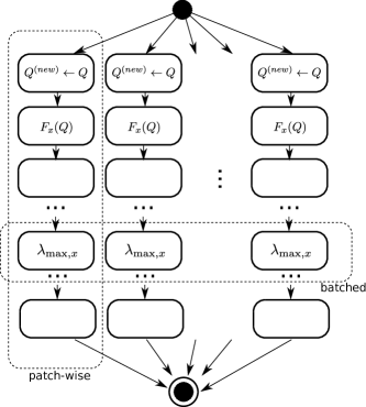
Figure 1: Sketch of the compute graph sketch for a kernel over $T$ patches. Each node in the graph represents a $d$-dimensional loop over all volumes of the patch subject to halo volumes where appropriate.

There is a multitude of ways to translate Alg. 1 into SYCL. We start from a rewrite of the algorithm into a directed, acylic graph (DAG) over sets of calculations per patch (Fig. 1). Each node within this DAG equals a $d$-dimensional loop over microkernel calls. It can be vectorised, i.e. facilitates coalesced memory access.

Definition 2.

A patch-wise realisation employs a (parallel) outer loop running over the patches. Within each loop “iteration”, one patch is handled.

Patch-wise kernels group the calculations vertically (Fig. 1). An outer loop handles the set of patches patch by patch. While this outer loop yields parallelism over the patches—the SYCL code is very close to Alg. 1 where the outer loop over $patch$ is running in parallel—there are additional (nested) parallel loops over $c$. Their ends synchronise the logical steps of Alg. 1 on a per-patch base: After we have done all the flux calculations along the x-direction for one patch, we continue with all the calculations along y. This synchronisation is totally independent of the flux calculations for any other patch. Only the very end implements a global synchronisation that coincides with the end of the loop over the patches.

Globally, the execution graph fans out initially with one branch per patch, and it fans in once in the end. Within each fan branch, the steps run one after the other. However, each step fans in and out again. The concurrency level within the kernel hence always oscillates between $T$ and $\mathcal{O}(T(p+2)^{d})$ with only one global synchronisation point in the end.

Definition 3.

A batched realisation runs over the logical algorithm steps one-by-one. Within each step, it processes all volumes from all patches in parallel.

This scheme clusters calculations horizontally (Fig. 1). It realises the kernel as a sequence of algorithmic steps. Within each step, we update all volumes from all patches concurrently. After each step, we synchronise over all patches. The scheme is labelled as batched [7], inspired by batched linear algebra [1], while we use the same (non-linear) operator (matrix) for each patch input $Q$.

Globally, we get a trivial DAG enlisting the calculation steps like pearls in a row. Each step within the DAG fans in and and out, i.e. has an internal concurrency level in the order $\mathcal{O}(T\cdot(p+2)^{d})$. As we bring the algorithmic steps into an order, i.e. remove concurrency from the global DAG by partial serialisation, there are multiple synchronisation points.

Definition 4.

The task-graph realisation employs one task graph where each node represents all operations (microkernel calls) of one type for one patch.

The task-graph approach is a plain realisation of the logical task graph (Fig. 1). Each individual node within this task graph fans in and out and has an internal concurrency of $\mathcal{O}((p+2)^{d})$, and we may assume that there are always at least $T$ nodes ready.

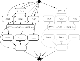
Figure 2: Partial sketch of the task graph fed into the task-graph realisation.

Different activities (types of microkernels) within the DAG can run in parallel. An example is the calculations of the directional fluxes $F_{x}(Q)$, $F_{y}(Q)$ and $F_{z}(Q)$ that have no dependencies. Both the batched variant and the patch-wise variant serialise these three steps; the former globally and the latter on a patch basis. It is the task-graph approach that does not go down this route and exposes the concurrency explicitly (Fig. 2).

4 SYCL implementation

Conceptually, mapping either of the three realisations onto SYCL is straightforward. There are subtle details to consider however.

Kernels

The batched variant yields a sequence of SYCL command group functions. They are submitted to a queue and executed in-order. The synchronisation points currently are realised via waits on the events returned by a kernel launch, i.e. each SYCL submission waits for the required predecessors to terminate. Different command groups thus may run in parallel, but each handles all volumes of all patches subject to one microkernel only. We do not tie our implementation to an in-order queue, for which we could omit the waits.

Each command group hosts one large parallel for iterating over all patches times all finite volumes within the patches. Depending on the step type, we might have further embedded loops over the (flux) direction and the unknowns (for the copy kernel). We end up with a cascade of $1+d+d=1+2d$ loops (patches, cells along each direction, flux along each direction). They are collapsed into one large loop.

The graph-based variant starts to spawn one SYCL command group per patch for the first algorithmic step. Each command group’s return event is collected in a vector. We continue to launch the next set of command groups for the next algorithmic step per patch, augment each submission with the corresponding event dependencies on the previously collected events—where required—and again gather the resulting events. The dynamic construction of the SYCL DAG resembles the batched variant code, where we replace the global waits with individualised dependencies. Each individual task within the graph-based variant hosts one parallel for that traverses a collapsed loop. The number of loops collapsed is smaller by one compared to the batched variant.

The patch-wise realisation of the kernel requires most attention. SYCL does not have direct support for nested parallel loops or sequences of loops within one kernel. Furthermore, we may only synchronise individual work groups. Therefore, we map the outer loop onto a parallel for over work groups via nd_range.

Idiom 1.

To support nested parallelism, we manually collapse the loops and issue one large parallel for over the resulting total loop range subject to an nd_range object. The nd_range decomposes the iteration range again into subranges that are independent of each other, i.e. correspond to the outer loop.

Idiom 2.

To support sequences of parallel loops within one kernel, we issue one parallel for subject to an nd_range. After each logical loop body, we use a workgroup barrier.

Idiom 3.

To support sequences of parallel loops with different ranges, we take the union of all iteration ranges. Per code snippet in-between two barriers, we manually mask out loop indices which are not required in this particular step, i.e. result from the union.

1 ::sycl::range$<4>$ total { T,2+p,2+p,2+p }

2 ::sycl::range$<4>$ workgroup { 1,2+p,2+p,2+p }

3 queue.submit( [&](::sycl::handler &handle) {

4 x handle.parallel_for(

5 xx ::sycl::nd_range$<4>${total, workgroup},

6 xx [=] (::sycl::nd_item$<4>$ i) {

7 xxx reconstruct $patch,c$

8 xxx if ($c_{x}\geq 0\wedge c_{x}\leq p-1$) compute $F_{x}(Q)(patch,c)$

9 xxx i.barrier()

10 xxx … // Next algorithmic step

11 xxx … // with different masking

12 xx })

13 });

Algorithm 2 Manual masking and concatenation of logical algorithmic steps for the patch-wise realisation.

As each patch is mapped onto a workgroup and work groups run concurrently, we add a workgroup barrier after each compute step on a patch (after each horizontal cut-through in Fig. 1). The iteration range per algorithmic step per workgroup is different from step to step, i.e. between any two barriers: A single flux computation for example runs over an iteration range of $(2+p)\cdot p^{d-1}$, while the subsequent update of a cell using all directional fluxes iterates over a range of $p^{d}$. Therefore, the workgroup loops over the maximum iteration range of $(2+p)^{d}$ right from the start, and we add if statements to mask out unreasonable computations manually (Alg. 2).

Data structure layout

The discussion of AoS vs. SoA is an all-time classic in supercomputing. In the context of Finite Volumes, SoA can yield significant speedups. However, we write our kernels around the notion of microkernels wrapping user functions for the PDEs. This commitment which allows us to separate the roles of domain scientists clearly from performance engineers [5] implies that AoS is the natural data structure for $Q$ in ExaHyPE: fluxes, eigenvalues, sources, …all are defined as functions over $Q$. Having all $N$ entries of $Q$ consecutively within the memory allows us to realise these operations in a cache efficient manner. Furthermore, many PDEs require the same intermediate results entering all components of $F_{x}(Q)$, e.g. Storing and traversing $Q$ as SoA would require us either to gather the $N$ entries first, or to recompute partial results redundantly.

For the temporary results, i.e. all the fluxes and eigenvalues, it is not clear if they should be stored in AoS or if the microkernels should scatter them immediately into SoA. They enter subsequent compute steps where SoA could be beneficial. Our realisation hence parameterises the microkernels further, such that we can use them with different storage formats: We augment the enumerator with a function $enum:[0,\ldots,T-1]\times[-1,0,\ldots,p]^{d}\times\mathbb{N}^{+}_{0}\mapsto\mathbb{N}^{+}_{0}$, such that they also take the unknowns into account.

Idiom 4.

Due to the absence of $d>3$-dimensional ranges within SYCL, we “artificially” map our higher-dimensional indices and ranges onto $d=3$-dimensional SYCL ranges.

While this is a workaround and higher-dimensional ranges in SYCL are promised for future language generations, the manual partial linearisation allows us to anticipate the order of the fastest running index within $enum$, such that all memory accesses are coalescent.

Reduction

Native SYCL reductions for the eigenvalue reduction are available when we work with the task graph realisation: We launch one dedicated SYCL command group with a reduction per patch. For the batched variant, we have to abandon the parallel_for over a range, and instead launch the for over an nd_range similar to the patch-wise solution. Within the for loop, we use the reduce_over_group variant. The patch-wise variant finally is able to use the reduction over the group, too. However, the manual masking has to be mapped onto a branching that returns the neutral element, i.e. $\max(\lambda_{\text{max},x}(Q),\lambda_{\text{max},y}(Q),\lambda_{\text{max},z}(Q))=0$.

Without reduce_over_group, it is possible to realise the reduction via atomics or to run through each patch serially. A serial implementation means that the batched flavour launches a parallel for over the patches (concurrency $T$) yet uses a plain nested C for loop for the reduction itself. For the patch-wise implementation it means that only the 0th thread per patch aka workgroup performs this loop. All the others are masked out. We use the parallel variant.

Data transfer

SYCL offers USM. Hence, we can run all kernel variants directly on the GPU, as long as the underlying data structures are allocated via malloc_shared. The responsibility to transfer all data then is deployed to the runtime. Alternatively, we can copy data forth and back explicitly. Remote GPU allocations issued by the host, as required by an explicit copy, are expensive in OpenMP [12]. Assuming similar patterns arise for SYCL, we implement managed memory, where we allocate memory explicitly on the GPU yet do not free it once a kernel has terminated. Instead, we recycle this memory.

For the batched kernel variant, there is limited freedom to overlap memory transfer and kernel kick off. The piece-wise and the DAG variant however allow the kernels to overlap by kicking off one patch’s computations while data for the second patch is still dropping in. Explicit copying and the managed memory eliminate this advantage, as they are realised as preamble to the compute kernel launch, but USM plus patch-wise or DAG flavour allow for overlaps of computations and data transfer.

Code change complexity

All three realisation flavours have to be maintained separately. As we rely on the notion of a microkernel and can extract common features such as the enumerations, the allocation of temporary data structures, or the actual data transfer (if required) into helper functions, each manifests in a few hundred lines of code realising the core SYCL task or loop structure.

The structure of the batched realisation in SYCL resembles 1:1 a plain C++ implementation subject to the additional queue submits and waits. The patch-wise variant is similar to its C++ counterpart, yet requires one additional barrier per algorithmic step plus the additional masking (if statements). This corresponds to two lines of additional code per algorithm step and an increased logical complexity to keep track of the correct masking. The task-graph version resembles the batched variant but does not wait for any outcome: The tasks are spawned in the same order as in the batched variant, the task completion events are stored in one STD vector per algorithm step, and additional depends_on calls insert the dependency graph’s edges using the previously populated vectors. The task logic—although not trivial—materialises in one or two lines of code per algorithmic step. All task graph construction is dynamic and hence enters the kernel runtime cost.

5 Results

Our present work studies exclusively the Euler equations ($N=2+d$) and drops the non-conservative terms $\boldsymbol{\mathcal{B}}_{i}=0$ as well as the point ($\delta=0$) and volumetric ($\textbf{S}(Q)=0$) sources from (1). All timings present the compute time for $T$ patches on the GPU, and we typically use $p\in\{4,6,8\}$. All measurements are averaged over at least 16 samples.

We ran our experiments on an A100 NVIDIA GPU. The card runs at 1,056 MHz, and it features 80GB of HBM2e memory. Further to that, we also run all experiments on one stack (half of)) of a Intel Data Center GPU Max 1550 (Ponte Vecchio) equipped with 128 GB of HBM2e memory and clocked at a base frequency of 1,000 MHz.

For all experiments, we employed the 2023.2.0 oneAPI software stack with Intel’s LLVM compiler. On NVIDIA, the Codeplay plugin was added to enable the CUDA backend for SYCL, whereas the Intel hardware is supported out of the box (Level Zero). Our experiments with CUDA unified memory crash immediately due to an error in the CUDA layer. On the PVC, the USM realisations pass, although we had to disable advanced features (Appendix D). We note that both the CUDA software stack and the PVC driver and BIOS are still in active development. An improved stability might lead to quantitatively different results in the future.

Patch-wise kernels

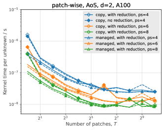
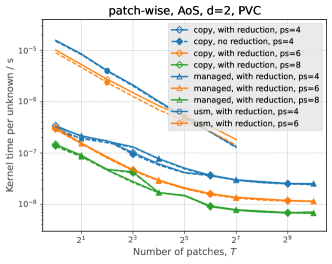
Figure 3: Cost per degree of freedom update for various $p$ and $T$ choices for $d=2$ on an NVIDIA A100 (top) or Intel PVC (bottom). Patch-wise realisation.

We start with an assessment of the patch-wise strategy for different $p$ values and $T$ choices (Fig. 3). AoS is used for all input, output and intermediate data structures. Our experiments once run the kernel including the computation of a final maximum eigenvalue, before we rerun the same kernel again yet strip it off this final reduction. All timings incorporate data transfer.

Higher $p$ or $T$ counts reduce the cost per unknown update on both architectures and for all realisation flavours. The reduction increases the runtime, but the impact is almost negligible. As we increase the problem size, we would expect throughput improvements given the enormous hardware concurrency of the cards. Instead, the A100 data plateaus and exhibits deteriorated performance for some $p\cdot T$ combinations. The PVC is robust regarding outliers, but plateaus as well. All $d=3$ data are qualitatively similar, though the anomalies on the A100 are more pronounced. Explicit copying and host-managed GPU memory both outperform USM on the PVC, but do not differ from each other. On the A100, it is advantageous to recycle memory.

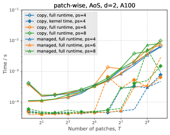
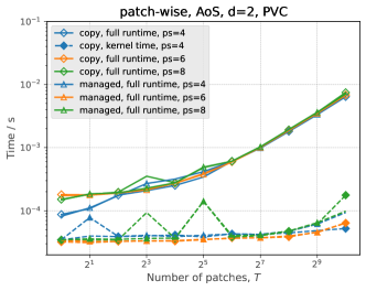
Figure 4: Breakdown of the total runtime for all patches from Fig. 3 into total kernel compute time and total kernel runtime including data transfer cost.

Our runtimes are dominated by data transfers (Fig. 4). ExaHyPE’s patches are scattered over the CPU’s heap memory and have to be brought to the accelerator one by one. The transfer cost suffers from the latency of multiple, scattered memory transfers. It therefore increases with $T$. Copying a single patch seems to be particularly expensive on the A100. Here, we benefit particularly from a managed memory approach. The compute time flatlines for small $T$. Once we increase $T$ sufficiently, also the compute time starts to grow. The PVC compute times peak for some small $T$ choices and $p=8$, while the A100 shows some runtime peaks for few larger $p\cdot T$ combinations. The latter explain the runtime “anomalies” in the total execution time.

Each patch is mapped onto a workgroup of its own. Increasing the workload $p$ per workgroup yields higher throughput, since the elementary workgroup workload is higher, i.e. we can do more calculations before we terminate or swap a workgroup. Furthermore, the share of iteration range indices that do not fit to the hardware’s workgroup size and hence have to be masked out diminishes. The thread divergence decreases. The PVC seems to be particular sensitive to these effects for small $p$. The A100 is sensitive to these effects when they are scaled up by using many patches $T$. The compute performance’s inital flatlining demonstrates that small choices of $T\cdot p$ struggle to exhaust the compute power.

Idiom 5.

Larger $d\cdot p$ combinations are infeasible due to workgroup size limits in SYCL (1,024 on both PVC and A100). Large patches $p$ have to broken down manually such that they fit onto the hardware.

We also conclude that USM—even ignoring the reported stability issues—is best to be avoided if we can copy explicitly. Notably, it fails to to benefit from overlapping computations and calculations. However, our implementation lacks the usage of prefetches which might help to make the USM implementation faster.

Batched kernels

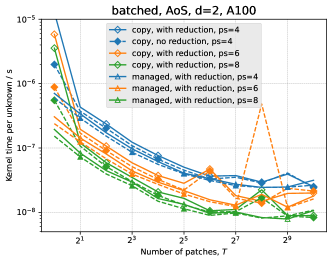
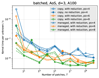
Figure 5: Normalised runtime for batched kernels on the A100 for $d=2$ (top) and $d=3$ (bottom).

The batched kernel variant yields performance curves on the A100 where the peaks are amplified. It also is significantly slower than the patch-wise approach for a single patch (Fig. 5). The PVC’s performance deteriorates totally for $T=1$ and for $d=3$ with larger $T\cdot p$ (Fig. 6). Here, we suffer from the cost of the reduction. For all other experiments, the batched variant catches up with its patch-wise cousin and eventually matches its performance on either machine as $T\cdot p$ grows.

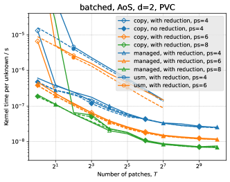
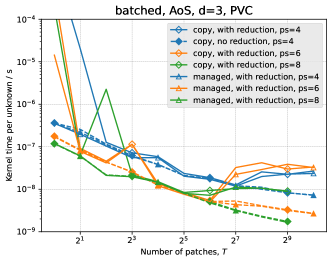
Figure 6: Normalised runtime for batched kernels on PVC for $d=2$ (top), and on PVC for $d=3$ (bottom). Deteriorated runtimes $t(T=1)\gg 4\cdot 10^{-5}$ are cut off to preserve a uniform scaling of the y-axes. USM data is omitted due to its non-competitiveness.

The GPU copes well with a large number of threads that all run the same computations, as SYCL can subdivide the iteration range into workgroups as fit for purpose. Per algorithmic step, the batched variant has no logical thread divergence, i.e. we do not mask out threads manually, although SYCL will add idle threads internally to make the iteration ranges match the hardware concurrency. A profiler indeed shows smaller workgroup sizes compared to the patch-wise version, i.e. more workgroups are created. Yet, the register pressure per workgroup is significantly smaller.

The ratio of idling threads per workgroup compared to the actual workload is smaller than for the patch-wise variant, and the arrangement of workgroups might even change between different algorithmic kernel steps. However, we pay a price for launching multiple GPU kernels in a row and the corresponding synchronisation points. The A100 seems to be particularly sensitive to this. $p\cdot T$ has to become reasonably large, before the increased flexibility plus the fewer “wasted” threads allow the batched version to compensate for the kernel launch overhead and to close up on the patch-wise realisation. While we do not have to care about maximum workgroup sizes for the kernel’s main compute steps, an efficient, parallel reduction of the final maximum eigenvalue continues to hinge on the fact if one patches fits into a workgroup. Even if this is the case, the PVC’s performance might suffer from reductions over large data sets.

Task-graph kernels

A straightforward implementation of our task graph approach does not scale at all in $T$ (Fig. 7). We observe qualitatively similar data for $d=2$ and $d=3$ on the A100. While increasing $p$ brings the relative runtime down, the performance immediately starts to stagnate and the resulting overall kernel remains significantly slower than the batched or patch-wise kernels. On the PVC, the performance does not stagnate but actually increases for growing $T$ after a brief scaling phase or the code deadlocks (no data shown). For $d=2$, the performance gap between USM and the other approaches eventually closes, but this is due to the poor performance of the latter rather than USM’s performance.

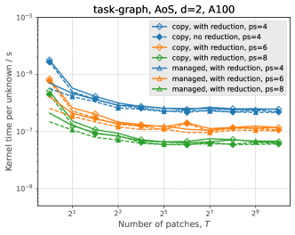
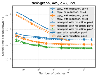
Figure 7: Kernel runtimes on the A100 (top) and the PVC (bottom) for a realisation using a SYCL task graph for $d=2$.

We assume that the dynamic assembly of the task graph, which is included in the compute kernel timings, is too expensive, as it maps each compute step within the DAG onto a separate kernel launch. The low arithmetic intensity of our individual computations amplifies this effect. Once $p$ increases and hence introduces reasonable high compute load per DAG step, the relative overhead reduces. The A100 profits from this fact, while the PVC continues to struggle with the high number of kernel launches. We conclude that a dynamic administration of the task graph on the host side is not competitive with our two alternative realisation variants.

While our code base should support dynamic numbers of $T$—we want to support dynamic AMR where we do not know a priori how many tasks are spawned and offloaded to the GPU per thread [7, 12]—the task graph is fixed once we decide to load a certain number $T$ of patches with a given $p$ to the accelerator. There is no need to assemble a task graph dynamically. Instead, we can precompile the graph, offload it to the GPU, and let the GPU handle the dependency administration internally. SYCL provides (experimental) extensions for this through task graph recording and explicit graph construction APIs. Unfortunately, we were not able to use them successfully with our current software stack. Instead, we use dynamic task graph assembly and let the assembly contribute towards the kernel runtime.

Further implementation remarks

We did extensive studies comparing SoA against AoS and also AoSoA, where the data data per patch are stored as SoA, while the individual patch data chunks are stored one after another. These ordering variations make no significant difference to the runtimes. Solely converting the input $Q$ into SoA increases the runtime dramatically, as we then have to gather data for each and every microkernel.

We use SYCL’s reduce_over_group for reductions wherever a plain reduction does not work. It yields a speedup of around a factor of two compared to a purely sequential version for small patches, and still a runtime improvement of around 10% for the larger $p$ values. An alternative parallel reduction using one atomic per patch is not competitive. No problem was scaled up to a point where SYCL’s workgroup size becomes a limiting factor, though this limitation is discussed.

In all kernels, we refrain from an explicit parallelisation over the unknowns in $Q\in\mathbb{R}^{N}$. Some loops over microkernels expose concurrency in the unknowns; to update all components according to an explicit Euler, e.g. However, exploiting this concurrency seems never to pay off, while it introduces massive (logical) thread divergence penalties in the patch-wise variant.

6 Outlook and conclusion

SYCL is still the new kid on the block when it comes to GPU programming. However, its “all-in-native-C++”–policy makes it attractive to projects that aim for code which runs both on CPUs and GPUs [3], and that aim to hide platform specifics by sticking to one language and one implementation only. It also is appealing, as it offers a task-first approach to heterogeneous programming: All kernel submissions can be considered to be tasks, return events, and can have dependencies.

Unfortunately, the flexibility promised by tasks seems not to pay off. Our data suggest that performance engineers have to embed the logical task graph into sequences of nested loops and map these loops onto one high-dimensional SYCL loop to obtain high performance. This is a low-level rewrite of the high-level task concept. We discuss two low-level realisations: batched and patch-wise. The patch-wise variant’s performance is robust for small problem sizes and very close to how domain scientists traditionally phrase their algorithms (run over all patches; per patch, compute …), but it requires some significant re-engineering and several workarounds if we implement it in SYCL. It is also subject to hardware (workgroup size) constraints. The batched version outperforms its patch-wise cousin for some bigger setups on some machine–dimension combinations.

Eventually, performance engineers might have to maintain two realisations to facilitate high throughput on a GPU: A patch-wise version for small $T$ counts, and a batched version for bespoke, larger setups; which are time-consuming by definition. On the CPU, a task-based version might be advantageous, which adds a third implementation variant. It will be subject of future work to investigate if this pattern changes with new hardware and software generations, i.e. if SYCL’s native task formalism catches up performance-wisely. As it stands, maintaining different realisations of one and the same numerical kernels remains necessary though being tedious and error-prone.

A fast, native, task-first USM programming paradigm for GPUs would be another real selling point for SYCL. As it stands, platform-portability might be guaranteed for the most generic and flexible way to phrase computations, but performance sacrifices have to be made if we want to use a strict task formalism and do not want to administer or copy data ourselves.

On the low-level realisation side, SYCL offers a GPU abstraction somewhere halfway in-between OpenMP and CUDA: Some details such as the orchestration of collapsed loops are hidden (like in OpenMP), while they can be exposed and tailored towards the machinery explicitly by using nd_ranges. Our work showcases that some codes would benefit from an even higher level of abstraction. It is not clear why SYCL does not provide stronger support for nested parallel fors as we get them natively in OpenMP, it is not clear why the maximum workgroup size of the hardware imposes constraints on the implementation and cannot be mitigated within the SYCL software layer, and a better support for nested parallelism and the automatic serialisation over some iteration indices (i.e. of loops over unknowns) would streamline the development.

While our work makes statements on efficient compute kernel realisations, it falls short of examining the impact of further advanced realisation techniques such as memory prefetching and task graph recording plus re-usage. It might be possible that such invasive techniques—in the sense that more manual source code augmentation becomes necessary—allow us to close the performance gap between USM and manual memory movements as well as on-the-fly task graph construction and task graph processing. Further to studying these features, future work will comprise data layout optimisations beyond simple reordering of temporary data and the optimisation of the core calculations. As long as we stick to the policy that no user code is altered, our code is inherently tied to AoS and the physics calculations are locked away from further tuning. If we want to keep the strict separation of roles, it hence might become necessary to switch to domain-specific languages, such that the translator has the opportunity to alter both the kernel and the microkernels.

Appendix A Download and build

All of our code is hosted in a public git repository on https://gitlab.lrz.de/hpcsoftware/Peano and available to clone. Our GPU benchmark scripts are merged into the repository’s main, i.e. all results can be reproduced with main branch. Yet, to use the exact same code version as used for this paper, please switch to tag a3461cb6 on the gpu branch.

1 git clone -b gpus https://gitlab.lrz.de/hpcsoftware/Peano

2 cd Peano

3 libtoolize; aclocal; autoconf; autoheader; cp src/config.h.in .

4 automake –add-missing

Bash commands 3 Cloning the repository and setting up the autotools environment.

1 ./configure CC=icx CXX=icpx LIBS=”-ltbb” LDFLAGS=”-fsycl -fsycl-targets=nvptx64-nvidia-cuda -Xsycl-target-backend=nvptx64-nvidia-cuda –cuda-gpu-arch=sm_80” CXXFLAGS=”-O3 -std=c++20 -fsycl -fsycl-targets=nvptx64-nvidia-cuda -Xsycl-target-backend=nvptx64-nvidia-cuda –cuda-gpu-arch=sm_80” –with-multithreading=tbb –enable-exahype –enable-blockstructured –enable-loadbalancing –with-gpu=sycl

2

3./configure CC=icx CXX=icpx LIBS=”-ltbb” LDFLAGS=”-fsycl” CXXFLAGS=”-O3 -std=c++20 -fsycl” –with-multithreading=tbb –enable-exahype –enable-blockstructured –enable-loadbalancing –with-gpu=sycl

Bash commands 4 Configure command used for our A100 tests (top) and for the PVC runs (middle).

While the project supports CMake as discussed in the project documentation (available by running doxygen documentation/Doxyfile), we present the setup using autotools here (Commands 3). To create the actual makefiles for A100 tests, initialise the oneAPI environment or use your native oneAPI modules, and afterwards configure your code accordingly (Commands 4). You will obtain a plain makefile that builds all of Peano’s and ExaHyPE’s core libraries.

Appendix B Execution and postprocessing

All experiments as discussed are available through a Python script that links a test case driver (miniapp) to Peano’s and ExaHyPE’s core libraries. This miniapp sweeps through the parameter combinations of interest for the present discussions.

1 cd benchmarks/exahype2/euler/kernel-benchmarks

2 python kernel-benchmarks-fv-rusanov.py –dim 3 –patch-size 8

Bash commands 5 Build a $d=3$ setup with patches of size $8\times 8\times 8$. The Python script internally invokes make (or cmake if you have previously configured the code with CMake) and yields an executable ./kernel-benchmark-fv-Xd-patch-size-Y where X is the dimension (3 in this example) and $Y$ the patch size (8).

To build the miniapp, we change into Euler’s kernel-benchmarks folder. The Python 3 script kernel-benchmarks-fv-rusanov.py yields the test case executable (Commands 5). Passing -h provides instructions on various further options. For example, the test can be asked to validate the GPU outputs for correctness against a CPU run, or you can alter the number of samples taken, i.e. over how many runs the measurements should average.

1 export ONEAPI_DEVICE_SELECTOR=level_zero:0

2 for i in 4 6 8; do

3 python kernel-benchmarks-fv-rusanov.py -d 3 -ps $i

4 ./kernel-benchmarks-fv-rusanov-3d-patch-size-$i $>$ pvc-3d-ps$i.txt

5 done

6

7python create-exahype-sycl-plot.py -f pvc-3d-ps4.txt pvc-3d-ps6.txt pvc-3d-ps8.txt -d 3 -ds AoS -ps 4 6 8 -dn PVC

Bash commands 6 Run benchmarking executable, pipe the outcome into a text file, and produce a graph through matplotlib. This example will produce an AoS plot for each implementation plus a comparison of the total runtime and the compute kernel time. The ONEAPI_DEVICE_SELECTOR environment variable chooses the target offload device which, in this case, is the first PVC GPU shown after running sycl-ls. The text files can be reused for other plots by rerunning the plotting script with different specifications.

The directory contains an example SLURM script, compile-and-plot.sh. It compiles and run the executable and pipe the output into a txt file, then finally feeds the output into a matplotlib script (create-exahype-sycl-plot.py) to produce the outputs. If you prefer to run the examples directly, follow the instructions 6.

Appendix C AoS, SoA and AoSoA

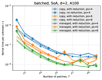
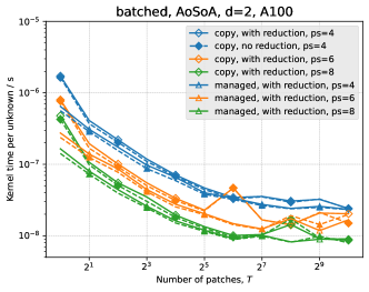
Figure 8: $d=2$ results on an NVIDIA A100 using different data layouts within the batched kernels.

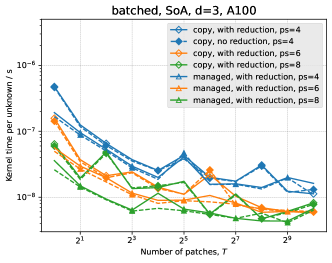
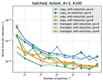
Figure 9: $d=3$ results on an NVIDIA A100 using different data layouts within the batched kernels.

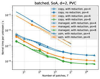
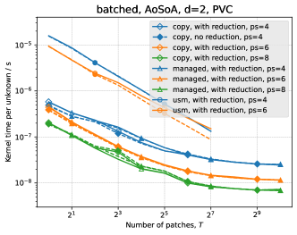
Figure 10: $d=2$ results on the PVC using different data layouts within the batched kernels.

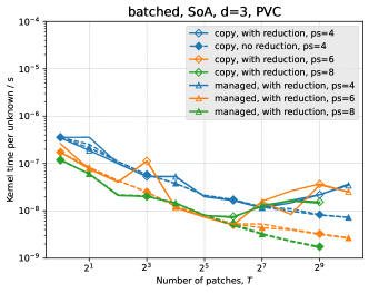
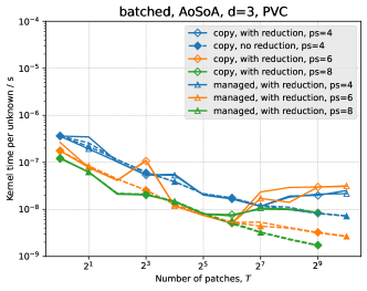
Figure 11: $d=3$ results on the PVC using different data layouts within the batched kernels.

Data on the runtime impact of AoS vs. SoA and a further hybrid (AoSoA) confirms our statement that the organisation of temporary data has negligible impact on the runtime (Figures 8, 9, 10, and 11). We observe that the characteristic dips for $p=4,d=2$ on the PVC appears independently of the data layout chosen for the temporary fields.

Appendix D Machine settings

On Intel’s Data Center GPU Max Series—abbreviated by PVC in the plots, as the previous codename has been Ponte Vecchio—we use the level-Zero API. We use only a subset of the available features of the chip (Alg. 7).

1 export EnableImplicitScaling=0

2 export ZE_AFFINITY_MASK=0.0

3 export ZE_FLAT_DEVICE_HIERARCHY=FLAT

4 export SYCL_PI_LEVEL_ZERO_USE_COPY_ENGINE=0

Algorithm 7 Environment variables used on PVC.

The chip features 1,024 Xe Vector engines organised into two stacks. We use only one stack and disable implicit scaling. That is, we do not even allow the chip to make use of the second stack’s memory and other resources. The affinity settings ensure that only this first half of the card is visible to the tests, while it is exposed as one flat, uniform device.

Our testbed struggled to benefit from the PVC’s copy engine. We therefore explicitly disable this feature throughout the tests, which might negatively affect the USM throughput.

Future driver and software stacks will likely allow users to avoid tinkering with environment variables. Future hardware and software generations also will enable SYCL USM on the A100. However, we do not expect large quantitative differences in the outcomes and notably doubt that the significant performance gap between USM and manual data transfer variants can be closed.

For researchers who want to reproduce results, it is important to note that our test driver covers all functional variations of the compute kernels. If features make the code crash or deadlock, the reproducer benchmark will hence not pass either. In this case, the respective kernel invocations in the file KernelBenchmarksFVRusanov-main.cpp have to be commented out.

References

- [1] A. Abdelfattah et al. A set of batched basic linear algebra subprograms and lapack routines. ACM Transactions on Mathematical Software, 47(3):1–23, 2020.
- [2] D.E. Charrier, B. Hazelwood, and T. Weinzierl. Enclave tasking for dg methods on dynamically adaptive meshes. SIAM Journal on Scientific Computing, 42(3):C69–C96, 2020.
- [3] T. Deakin et al. Heterogeneous programming for the homogeneous majority. In IEEE/ACM International Workshop on Performance, Portability and Productivity in HPC, P3HPC@SC 2022, Dallas, TX, USA, November 13-18, 2022, pages 1–13. IEEE, 2022.
- [4] A. Dubey et al. A survey of high level frameworks in block-structured adaptive mesh refinement packages. Journal of Parallel and Distributed Computing, 74(12):3217–3227, 2016.
- [5] J.-M. Gallard et al. Role-oriented code generation in an engine for solving hyperbolic pde systems. In Tools and Techniques for High Performance Computing, pages 111–128, 2020.
- [6] M. Klemm and J. Cownie. High Performance Parallel Runtimes. De Gruyter Textbook, 2021.
- [7] B. Li et al. Dynamic task fusion for a block-structured finite volume solver over a dynamically adaptive mesh with local time stepping. In ISC High Performance 2022, volume 13289 of Lecture Notes in Computer Science, pages 153–173, 2022.
- [8] A. Reinarz et al. Exahype: An engine for parallel dynamically adaptive simulations of wave problems. Computer Physics Communications, 254:107251, 2020.
- [9] J. Reinders et al. Data Parallel C++: Mastering DPC++ for Programming of Heterogeneous Systems using C++ and SYCL. Springer, 2021.
- [10] C. R. Trott et al. Kokkos 3: Programming model extensions for the exascale era. IEEE Trans. Parallel Distributed Syst., 33(4):805–817, 2022.
- [11] T. Weinzierl. The peano software - parallel, automaton-based, dynamically adaptive grid traversals. ACM Transactions on Mathematical Software, 45(2):14:1–14:41, 2019.
- [12] M. Wille et al. Efficient GPU offloading with OpenMP for a hyperbolic finite volume solver on dynamically adaptive meshes. In ISC High Performance 2023, volume 13289 of LNCS, pages 153–173, 2023.