Spectroscopic comparative study of the red giant binary system gamma Leonis A and B

Abstract

$\gamma$ Leo is a long-period visual binary system consisting of K0 iii (A) and G7 iii (B) giants, in which particular interest is attracted by the brighter A since the discovery of a planet around it. While detailed spectroscopic comparative study of both components would be worthwhile (e.g., for probing any impact of planet formation on chemical abundances), such a research seems to have been barely attempted as most available studies tend to be biased toward A. Given this situation, the physical properties of A and B along with their differences were investigated based on high-dispersion spectra in order to establish their stellar parameters, evolutionary status, and surface chemical compositions. The following results were obtained. (1) The masses were derived as $\sim 1.7$ $M_{\odot}$ and $\sim 1.6$ $M_{\odot}$ for A and B, respectively, both of which are likely to be in the stage of red clump giants after He-ignition. The mass of the planet around A has also been revised as $m_{\rm p}\sin i_{\rm p}\simeq 10.7M_{\rm Jupiter}$ (increased by $\sim 20\%$). (2) These are normal giants of subsolar metallicity ([Fe/H] $\sim-0.4$) belonging to the thin-disk population. (3) A as well as B show moderate C deficiency and N enrichment, which are in compatible with the prediction from the standard stellar evolution theory. (4) The chemical abundances of 26 elements are practically the same within $\lesssim 0.1$ dex for both components, which implies that the surface chemistry is not appreciably affected by the existence of a planet in A.

Keywords  stars: abundances – stars: binaries: visual – stars: evolution – stars: individual ($\gamma$ Leo A and B) – stars: late-type

1 Introduction

The star $\gamma$ Leo (Algieba) is a well-known 2nd-magnitude star in the constellation Leo, which is known to be a visual binary consisting of two rather similar orange–yellowish stars (the brighter component $\gamma$ Leo A = $\gamma^{1}$ Leo = HD 89484 = HR 4057 with $V=2.37$ mag and the fainter component $\gamma$ Leo B = $\gamma^{2}$ Leo = HD 89485 = HR 4058 with $V=3.64$ mag) separated by a few arcseconds after the discovery of Sir William Herschel in 1782. Since this system has a highly eccentric orbit (eccentricity as large as $e\sim 0.9$) with very long period (several centuries), even half of its orbit has not been completed (neither periastron nor apoastron has been reached) over the past 240 years, which means that its orbital elements still suffer considerable uncertainties.

Modern astronomical spectroscopy revealed that these component stars are red giants classified as K0 iii (A) and G7 iii (B); that is, the brighter former is somewhat redder than the fainter latter. As these are apparently ordinary red giant stars like many others, this system was not of particular astrophysical interest for a long time, despite that it has been popular among amateur astronomers challenging to resolve it into two stars and to enjoy the delicate contrast of colors by using small home telescopes or binoculars.

However, a significant feature was recognized in this star about a decade ago, when Han et al. (2010) reported (based on the radial velocity method) the detection of a planetary companion with a mass of $m_{\rm p}\sin i_{\rm p}=8.78M_{\rm Jupiter}$ orbiting around $\gamma$ Leo A with a period of 429 days. This is an important finding because it is presumably the first planet-hosting visual binary of two similar red giants which are separately observable.

Generally speaking, a binary system in which only one component harbors a planet (while the other does not) is potentially an important testing bench for investigating the impact of planet formation on the host star, if the spectra of both stars are independently obtainable and their spectral types are not very different. That is, if any difference in the chemical abundances could be detected between the two, it would provide us with valuable information on the star–planet connection (e.g., accretion of proto-planetary materials), since they should have formed from gas with the same composition.

Although not a few such comparative studies of chemical abundances for the planet-host and non-planet-host components of visual binaries have been conducted so far, they are restricted to solar-type dwarfs such as 16 Cyg A+B and HD 219542 A+B (see, e.g., Ryabchikova et al. 2022 and the references therein). In this sense, it is worth determining the chemical abundances of many elements for $\gamma$ Leo A and B, in order to check whether any significant difference exists between these giant stars.

However, few such chemical abundance studies directed to both of $\gamma$ Leo A and B have been published. That is, most investigations on $\gamma$ Leo tend to be biased toward the brighter A, while little attention has been paid to the fainter B. As a matter of fact, as summarized in Table 1, only two rather old studies are available that included $\gamma$ Leo B (and also $\gamma$ Leo A) as one of the targets: (i) Lambert & Ries’s (1981) work on the CNO(+Fe) abundances of 32 G–K giants, and (ii) McWilliam’s (1990) abundance determinations of $\sim 10$ comparatively heavier elements (Si through Eu) for an extensive sample of 671 GK giants.

Table 1 : Stellar parameters of $\gamma$ Leo A and B reported in past publications.

Authors	$T_{\rm eff}$	$\log g$	$v_{\rm t}$	[Fe/H]	$M$	Remark
($\gamma$ Leo A)
Tomkin et al. (1975)	4300	1.7	1.7			12C/13C = 6.5
Lambert & Ries (1981)	4650	2.39	2.0	$-$0.35
McWilliam (1990)	4470	2.35	2.4	$-$0.49
Dyck et al. (1998)	3949					from interferometry-based angular diameter
aKovtyukh et al. (2006)	4306					assumed to be $\gamma$ Leo A (though labeled as HD 89485)
Cenarro et al. (2007)	4470	2.12		$-$0.38
Massarotti et al. (2008)	4365	2.3		$-$0.49
Han et al. (2010)	4330	1.59	1.5	$-$0.51	1.23
Prugniel et al. (2011)	4426	1.84		$-$0.38
Maldonado et al. (2013)	4372	1.66	1.43	$-$0.44	1.50
Santos et al. (2013)	4428	1.97	1.74	$-$0.41
Jofré et al. (2015)	4465	2.12	1.92	$-$0.51		$v_{\rm e}\sin i=2.36$ km s-1
Sousa et al. (2015)	4395	1.66	1.67	$-$0.47	1.46
ada Silva et al. (2015)	4454	1.91	1.63	$-$0.42	c(0.75)	assumed to be $\gamma$ Leo A (though labeled as HD 89485)
Maldonado & Villaver (2016)	4376	1.67	1.43	$-$0.44	1.59
bJönsson et al. (2017)	4341	1.77	1.56	$-$0.48		labeled as HIP 50583 $\rightarrow$ understood as $\gamma$ Leo A
bLomaeva et al. (2019)	4341	1.77	1.56	$-$0.45		labeled as HIP 50583 $\rightarrow$ understood as $\gamma$ Leo A
Charbonnel et al. (2020)	4274			$-$0.54	1.77	$A$(Li) = $-0.58$
($\gamma$ Leo B)
Lambert & Ries (1981)	5110	2.76	2.0	$-$0.37
McWilliam (1990)	4980	2.98	2.5	$-$0.52

Summarized here are the effective temperature (in K), logarithmic surface gravity in c.g.s unit (in dex), microturbulence (in km s^-1), Fe abundance relative to the Sun, and mass (in $M_{\odot}$) taken from various previous studies.
^aAlthough the star is labeled as HD 89485 (which literally means $\gamma$ Leo B) in their table, it is suspected to be a mistype of HD 89484 ($\gamma$ Leo A) as judged from the given $T_{\rm eff}$ value as low as $\lesssim 4500$ K. Besides, it seems rather unnatural to do an analysis only for the fainter B without touching the brighter A. Therefore, it is tentatively assumed that these data should be understood as those of $\gamma$ Leo A.
^bAlthough the star is labeled simply as HIP 50583, this number in the Hipparcos catalogue corresponds to $\gamma$ Leo A+B system as a whole (not the individual components). Therefore, it is assumed here that these data are those of the brighter $\gamma$ Leo A.
^cPresumably, some kind of error is involved in this mass value, which is too low.

Our group has so far published a series of papers focusing the abundances of various elements for a large sample of red giant stars: Takeda et al. (2008; hereinafter referred to as T08) [atmospheric parameters and abundances of many elements], Takeda & Tajitsu (2014; T14) [Be abundances], Takeda et al. (2015; T15) [C, O, and Na abundances], Takeda et al. (2016; T16) [S and Zn abundances], Takeda & Tajitsu (2017; T17) [Li abundances], and Takeda et al. (2019; T19) [¹²C/¹³C ratios and N abundances]. However, neither $\gamma$ Leo A nor B were included in our previous targets. Therefore, this unsatisfactory situation motivated the author to newly carry out a detailed spectroscopic comparative study of both $\gamma$ Leo A and B in order to compare the chemical abundances for a number of elements (volatile as well as refractory elements) between these planet-host and non-planet-host components, while making good use of our past experiences. This was the first motivation of this investigation.

Besides, by taking this opportunity, we intend to clarify the stellar parameters and the properties (e.g., activity level, kinematic information, etc.) of these two binary components, because they are not necessarily well established. Especially, although information of the stellar mass is important (which controls the stellar evolution and directly affects the mass evaluation for the orbiting planet), published results are rather diversified ($M$ of $\gamma$ Leo A ranges from $\sim 1.2M_{\odot}$ to $\sim 1.8M_{\odot}$; cf. Table 1). It should thus be worthwhile to determine the masses of both A and B as precisely as possible, such as attempted recently by Takeda (2022). for giants in the Kepler field.

In addition, we can also check the nature of internal mixing in $\gamma$ Leo based on the surface abundances of light elements (especially C, N, O, and Na). Our previous studies (T15 and T19) suggested that the surface abundance characteristics of mid-G to early-K giants (i.e., moderate deficiency in C, near-normal O, enrichment in N, mild overabundance in Na) are almost consistent with the results of recent theoretical simulations for red giants having experienced the first dredge-up (e.g., Lagarde et al. 2012). Meanwhile, some previous work on $\gamma$ Leo A done in 1990s reported that the surface abundances of the relevant light elements are anomalous and in conflict with the standard theory. That is, nitrogen is nearly normal ([N/Fe] $\sim-0.1$; Shavrina et al. 1996a) and carbon is even somewhat overabundant ([C/Fe] $\sim+0.2$; Shavrina et al. 1996b); this tendency is apparently incompatible with the results corroborated in our past papers. Is $\gamma$ Leo A a peculiar star in comparison with other red giant stars in general? To clarify this point is also counted as one of the tasks of this investigation.

2 Observational data

The observational data (high-dispersion spectra) employed in this study were obtained in two observatories: Okayama Astrophysical Observatory (OAO) and Subaru Telescope (Subaru). Actually, most of the analysis was done based on the former OAO spectra covering the visible (and near IR) wavelength region, while the latter Subaru spectra in the violet–UV region were subsidiarily used only for the specific purposes of Be abundance determination (from Be ii 3131) and measurement of Ca ii 3934 core emission.

2.1 OAO observation

The spectroscopic observations of $\gamma$ Leo A and B in the visible to photographic IR wavelength region were done in 2010 May 3 (UT) by using HIDES (HIgh Dispersion Echelle Spectrograph) placed at the coudé focus of the 188 cm reflector at Okayama Astrophysical Observatory. The exposure times were 300 s (A) and 1200 s (B). Equipped with three mosaicked 4K$\times$2K CCD detectors at the camera focus, HIDES enabled us to obtain an echellogram covering $\sim$ 5100–8800 Å with a resolving power of $R\sim 67000$ (with the slit width of $200~{}\mu$m).

2.2 Subaru observation

The Subaru observations of $\gamma$ Leo A and B were carried out on 2010 May 25 (UT) with HDS (High Dispersion Spectrograph) placed at the Nasmyth platform of the 8.2-m Subaru Telescope, by which high-dispersion spectra covering $\sim$ 3000–4600 Å could be obtained with two CCDs of 2K$\times$4K pixels in the standard Ub setting with the blue cross disperser. The spectrum resolving power was $R\simeq 60000$ with the slit width set at $0.^{\prime\prime}6$ (300 $\mu$m) and a binning of 2$\times$2 pixels. The integrated exposure times were 35 s (A) and 80 s (B), while the star lights were considerably reduced with the help of a neutral density filter in order to avoid saturation.

2.3 Data reduction

The reduction of the spectra (bias subtraction, flat-fielding, scattered-light subtraction, spectrum extraction, wavelength calibration, and continuum normalization) was performed by using the “echelle” package of the software IRAF in a standard manner.

3 Stellar parameters

3.1 Atmospheric parameters

The atmospheric parameters [effective temperature ($T_{\rm eff}$), surface gravity ($\log g$, where $g$ is in cm s^-2), and microturbulence ($v_{\rm t}$) were spectroscopically determined in the same manner as in T08 (see Sect. 3.1 therein for the details) based on the equivalent widths ($W_{\lambda}$) of Fe i and Fe ii lines measured on the OAO spectra covering $\sim$ 5100–8800 Å. The resulting parameters for $\gamma$ Leo A / $\gamma$ Leo B are $4457(\pm 23)$ / $4969(\pm 15)$ K, $1.89(\pm 0.10)$ / $2.53(\pm 0.05)$ dex, and $1.44(\pm 0.10)$ / $1.39(\pm 0.08)$ km s^-1, where $\pm$ values in parentheses are internal statistical errors (cf. Sect. 5.2 in Takeda et al. 2002). The Fe abundances ($A_{\rm Fe}$) corresponding to the final solutions are plotted against $W_{\lambda}$ and $\chi_{\rm low}$ in Fig. 1, where we can see that there is no systematic dependence as required. The detailed $W_{\lambda}$ and $A_{\rm Fe}$ data for each star are given in “feabunds.dat” of the supplementary material. The mean Fe abundances ($\langle A_{\rm Fe}\rangle$) for A / B are $7.09(\pm 0.03)$ / $7.12(\pm 0.02)$, where $\pm$ values in parentheses are the mean errors ($\epsilon\equiv\sigma/\sqrt{N}$; $\sigma$ is the standard deviation and $N$ is the number of lines). The corresponding values of metallicity ([Fe/H]) are $-0.41$ (A) and $-0.38$ (B). The model atmosphere for each star to be used in this study was generated by interpolating Kurucz’s (1993) ATLAS9 model grid in terms of $T_{\rm eff}$, $\log g$, and [Fe/H].

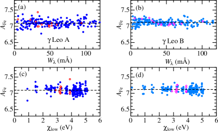
Fig. 1 : Upper panels (a) and (b): $A_{\rm Fe}$ (Fe abundance) vs. $W_{\lambda}$ (equivalent width) relations. Lower panels (c) and (d): $A_{\rm Fe}$ vs. $\chi_{\rm low}$ (lower excitation potential) relations. These Fe abundances correspond to the finally established atmospheric parameters of $T_{\rm eff}$, $\log g$, and $v_{\rm t}$ for $\gamma$ Leo A (left panels) and $\gamma$ Leo B (right panels). The filled and open symbols correspond to Fe i and Fe ii lines, respectively. The mean abundance ($\langle A_{\rm Fe}\rangle$) is indicated by the horizontal dashed line.

3.2 Mass and age

The absolute magnitude ($M_{V}$) or luminosity ($L$) are determinable from the apparent magnitude ($V$) and the parallax ($\pi$) with appropriate corrections, Then, since the position on the theoretical HR diagram is established in combination with $T_{\rm eff}$, the mass ($M$) as well as stellar age ($age$) can be evaluated with the help of theoretical evolutionary tracks.

For this purpose, the open software tool PARAM version 1.3 (da Silva et al. 2006) was employed as done by Takeda (2022), which requires $T_{\rm eff}$, [Fe/H], $V_{0}(\equiv V-A_{V})$, and $\pi$ (along with their errors) as input parameters (see Table 2). The uncertainty in $V-A_{V}$ was assumed to be 0.05 mag (that of $A_{V}$). The output results of $M$, $age$, $R$ (radius), and $\log g_{MR}$ (gravity from $M$ and $R$) are also summarized in Table 2.

For the sake of confirming these solutions, the positions of $\gamma$ Leo A and B on the $\log T_{\rm eff}$ vs. $\log L$ diagram are compared with the theoretical evolutionary tracks in Fig. 2, and the PARAM results of $age$ vs. $M$ relation are illustrated in Fig. 3.

Regarding the evolutionary status of these two stars, although it is difficult to discriminate based on these figures whether they are in the H-burning phase (ascending the red giant branch) or in the post-He-ignition phase (red clump giants), the latter would be more likely for both, because of the sign of advanced first dredge-up (such as the low ¹²C/¹³C ratio around $\sim 10$; cf. Sect. 5.1.2).

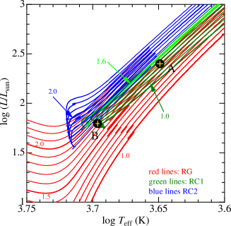
Fig. 2 : Positions of $\gamma$ Leo A and B (plotted by large filled circles with error bars indicated in yellow crosses) on the $\log T_{\rm eff}$–$\log L$ diagram, where Bressan et al.’s (2012) PARSEC tracks computed for $z=0.006$ (moderately metal-deficient by $-0.37$ dex lower than the solar metallicity) and various $M$ values (1.0, 1.1, 1.2, 1.3, 1.4, 1.5, 1.6, 1.7, 1.8, 1.9, 2.0, 2.1, 2.2, and 2.3 $M_{\odot}$; thick lines for the cases of integer masses, otherwise thin lines) are overplotted for comparison. These theoretical tracks are depicted in different colors corresponding to their evolutionary stages: Red $\cdots$ shell-H-burning phase before He ignition (Red Giant phase or RG). Green $\cdots$ $M\leq 1.8$ $M_{\odot}$ stars at the He-burning phase (1st Red Clump giant phase or RC1). Blue $\cdots$ $M>1.8$ $M_{\odot}$ stars at the He-burning phase (2nd Red Clump phase or RC2).

Fig. 3 : PARAM results of $age$ ($t$) and mass ($M$) for $\gamma$ Leo A and B plotted on the $age$–$M$ diagram, where $t_{\rm He*}$ (time of He-ignition) vs. $M$ relation (taken from PARSEC tracks) is also shown by the dashed line.

Fig. 4 : Observed residual flux spectra of Ca ii K line at 3933.663 Å are depicted by red lines for (a) $\gamma$ Leo A and (b) $\gamma$ Leo B. In addition, theoretical spectra ($r_{\lambda}^{\rm th}$) calculated from the model atmospheres with the assumption of LTE are also overplotted by blue lines. The core region (3932.8–3934.6 Å), where integration was done for evaluating the emission strength, is indicated by a horizontal bar. The wavelength scale is adjusted to the laboratory frame by correcting the radial velocity shift.

3.3 Stellar activity and rotation

In order to estimate the chromospheric activity, the activity index $\log R^{\prime}_{\rm Kp}$ was evaluated from the Subaru spectra by following the procedure described in Sect. 3 of Takeda et al. (2012) where $R^{\prime}_{\rm Kp}$ is the ratio of the chromospheric core emission flux of the Ca ii resonance line at 3933.663 Å (after subtraction of the photospheric flux computed from the classical model atmosphere) to the total bolometric flux. Fig. 4 displays the appearance of the spectra in the relevant core region of Ca ii 3934 line. The resulting $\log R^{\prime}_{\rm Kp}$ values are $-5.11$ (A) and $-5.07$ (B).

The projected rotational velocity ($v_{\rm e}\sin i$), which is closely related to stellar activity, was determined from the spectrum fitting analysis in the 6080–6089 Å region (cf. Fig. 5a and the top row of Table 3), as detailed in Sect. 4.2 of T08. The $v_{\rm e}\sin i$ results for $\gamma$ Leo A and B are 1.41 and 1.62 km s^-1, respectively.

Comparing these values of $\log R^{\prime}_{\rm Kp}$ and $v_{\rm e}\sin i$ with the trends shown in Fig. 6c–e of T17, we can see that both $\gamma$ Leo A and B are typical red giant stars of low activity for their low rotational velocities.

3.4 Kinematic parameters

The velocity components of a star and the properties of its orbital motion in the Galaxy are important to understand the stellar population. These kinematic parameters for the $\gamma$ Leo system (A and B do not need to be distinguished here) were obtained by following the procedure described in Sect. 2.2 of Takeda (2007), and the results are summarized in the last section of Table 2.

Plotting the resulting values of $V_{\rm LSR}$ (+11.7 km s^-1) and $z_{\rm max}$ (0.063 kpc) on the $z_{\rm max}$ vs. $V_{\rm LSR}$ diagram (cf. Fig. 5a of T17), we can state that $\gamma$ Leo belongs to the ordinary thin-disk population. This conclusion was also confirmed by applying the $U_{\rm LSR}$, $V_{\rm LSR}$ and $W_{\rm LSR}$ values to Bensby et al.’s (2005) kinematical criteria (cf. Appendix A therein), which yields $TD/D=0.05$ satisfying the criterion of $0<TD/D<1$ for thin-disk population.

Table 2 : Fundamental parameters of $\gamma$ Leo A and B adopted/derived in this study.

Quantity	(Unit)	$\gamma$ Leo A	$\gamma$ Leo B	Explanation
(atmospheric parameters determined from Fe i/Fe ii lines)
$T_{\rm eff}$	(K)	4457 ($\pm 23$)	4969 ($\pm 15$)	effective temperature
$\log g$	(dex)	1.89 ($\pm 0.10$)	2.53 ($\pm 0.05$)	surface gravity (in c.g.s.)
$v_{\rm t}$	(km s-1)	1.44 ($\pm 0.10$)	1.39 ($\pm 0.08$)	microturbulence
$[{\rm Fe/H}]$	(dex)	$-0.41$ ($\pm 0.03$)	$-0.38$ ($\pm 0.02$)	metallicity
(Gaussian macroturbulence and projected rotational velocity)
$v_{\rm mt}$	(km s-1)	3.03	2.60	based on 6080–6089 Å fitting (cf. Eq. 1 in T08)
$v_{\rm e}\sin i$	(km s-1)	1.41	1.62	based on 6080–6089 Å fitting (cf. Eq. 2 in T08)
(activity index)
$\log R^{\prime}_{\rm Kp}$	(dex)	$-5.11$	$-5.07$	see Eq. 2 in Takeda et al. (2012) for its definition
(photometric parameters)
$V$	(mag)	2.37	3.64	apparent magnitude in $V$-band (from SIMBAD)
$\pi$	(m.a.s.)	25.07 ($\pm 0.52$)	25.07 ($\pm 0.52$)	parallax from revised Hipparcos catalogue
$A_{V}$	(mag)	0.10 ($\pm 0.05$)	0.10 ($\pm 0.05$)	interstellar extinction from EXTINCT (Hakkila et al. 1997)
B.C.	(mag)	$-0.52$	$-0.27$	bolometric correction according to Alonso et al. (1999)
$\log(L/L_{\odot})$	(dex)	2.40	1.80	bolometric luminosity
(Parameters determined from evolutionary tracks)
$M$	($M_{\odot}$)	1.66 ($\pm 0.14$)	1.55 ($\pm 0.08$)	mass (by PARAM)
$age$	(Gyr)	1.75 ($\pm 0.43$)	2.12 ($\pm 0.33$)	age (by PARAM)
$R$	($R_{\odot}$)	26.08 ($\pm 0.79$)	10.55 ($\pm 0.29$)	radius (by PARAM)
$\log g_{MR}$	(dex)	1.80 ($\pm 0.04$)	2.56 ($\pm 0.04$)	surface gravity from $M$ and $R$ (by PARAM)
(kinematic parameters)
$v_{\rm r}^{\rm hel}$	(km s-1)	$-36.24$		heliocentric radial velocity (from SIMBAD)
$\mu_{\alpha}$	(m.a.s. yr-1)	$+304.30$		proper motion in $\alpha$ direction (from SIMBAD)
$\mu_{\delta}$	(m.a.s. yr-1)	$-154.28$		proper motion in $\delta$ direction (from SIMBAD)
$U_{\rm LSR}$	(km s-1)	84.2		radial component of space velocity at LSR (Local Standard of Rest)
$V_{\rm LSR}$	(km s-1)	11.7		tangential component of space velocity at LSR
$W_{\rm LSR}$	(km s-1)	3.6		vertical component of space velocity at LSR
$|v|_{\rm LSR}$	(km s-1)	85.1		$\sqrt{U_{\rm LSR}^{2}+V_{\rm LSR}^{2}+W_{\rm LSR}^{2}}$
$R_{\rm m}$	(kpc)	8.938		mean galactocentric radius
$e$	$\cdots$	0.262		orbital ellipticity
$z_{\rm max}$	(kpc)	0.063		maximum separation from the galactic plane

4 Determination of elemental abundances

4.1 Basic policy

In this study, larger weight is put to comparatively lighter elements (rather than heavier ones), because important volatile species or mixing-sensitive elements are included in this group. Therefore, abundances of such lighter elements are derived based on the spectrum-fitting method by taking the non-LTE effect into account, while abundance determinations for heavier elements are done by the conventional manner using equivalent widths with the assumption of LTE.

We exclusively focus on the relative abundances of $\gamma$ Leo A and B in comparison with the Sun ([X/H]_A or ([X/H]_B) along with their mutual differences ($\delta$[X/H]_A-B). Since they are derived by applying the differential analysis under the same condition (spectrum-fitting done in the same manner or differential line-by-line analysis based on equivalent widths) to the three spectra of A, B, and the Sun. uncertainties in atomic line parameters (especially those of oscillator strengths) are cancelled out and thus irrelevant.

4.2 Spectrum fitting analysis

Such as was conducted in T17, the abundances of 7 elements (Li, Be, C, O, Na, S, and Zn; either important lighter elements or volatile species) for $\gamma$ Leo A and B (as well as for the Sun) were determined by applying the spectrum-fitting technique, followed by a non-LTE analysis (except for several cases where LTE was assumed) based on the equivalent widths inversely derived from the best-fit abundance solutions (see Sect. 7–9 in T17 for more explanations of the procedures). Likewise, CN abundances (usable to obtain the abundances of N) and ¹²C/¹³C ratios were derived by the synthetic fitting method as done in T19.

Specific information (wavelength range, varied abundances, reference sources of the line data) regarding these spectrum fitting analyses is summarized in Table 3, and the atomic data for the representative key lines in each of the wavelength regions are presented in Table 4. Regarding the spectra for the Sun (to be used for deriving the reference solar abundances), the OAO spectra of Moon in the visible–near IR region (as in T15) and the Subaru spectra of Vesta in the UV–violet region (as in T17) were adopted.

How the theoretical and observed spectra match each other is displayed for each region in Fig. 5, and the results of the analysis (equivalent widths, non-LTE correction, elemental abundances, and differential abundances relative to the Sun) are summarized in Table 5.

Table 3 : Spectrum fitting analysis done in this study.

Purpose	Fitting range (Å)	Abundances varied∗	Atomic data source	Figure†
$v_{\rm e}\sin i$ determination	6080–6089	Si, Ti, V, Fe, Co, Ni	KB95 (cf. T08)	a
Li abundance from Li i 6708	6707–6708.5	Li, Fe, V	SLN98+VALD (cf. T17)	b
Be abundance from Be ii 3131	3130.45–3131.2	OH, Be, Ti, (Fe)fix	P97 (cf. T14)	c
C abundance from C i 5052	5051.3–5052.4	C, Cr, Fe, Ni	KB95m1	d
C abundance from C i 5380	5378.5–5382	C, Ti, Fe, Co	KB95 (cf. T15)	e
C abundance from C i 8335	8333.5–8336	C, Ti	KB95	f
C abundance from [C i] 8727	8726–8730	C, Si, Fe	KB95 (cf. T15)	g
CN and 12C/13C from CN lines	8001–8006	CN, Fe, 12C/13C	CCSM+SJIS (cf. T19)	h
O abundance from O i 7771–5	7770–7777	O, Fe, Nd, (CN)fix	TKS98+KB95 (cf. T15)	i
Na abundance from Na i 6161	6157–6164	Na, Ca, Fe, Ni	KB95 (cf. T15)	j
S abundance from S i 6757	6756–6758.1	S, Fe, Co	KB95 (cf. T16)	k
Zn abundance from Zn i 6362	6361–6365	O, Cr, Fe, Ni, Zn	KB95 (cf. T16)	l

^∗ The abundances of other elements than these were fixed by assuming [X/H] = [Fe/H] in the fitting.
^† Corresponding panel of Fig. 5.
CCSM — Carlberg et al. (2012), KB95 — Kurucz & Bell (1995), KB95m1 — Kurucz & Bell (1995) without the Fe i 5051.276 line, SLN98 — Smith, Lambert, & Nissen (1998), VALD — VALD database (Ryabchikova et al. 2015), P97 — Primas et al. (1997), SJIS — Sablowski et al. (2019), and TKS98 — Takeda, Kawanomoto, & Sadakane (1998).

Table 4 : Line data adopted for evaluating the equivalent widths.

Line	$W$	$\lambda$	$\chi_{\rm low}$	$\log gf$	Remark
		(Å)	(eV)	(dex)
Li i 6708	$W_{6708}$	6707.756	0.00	$-0.427$	7Li
		6707.768	0.00	$-0.206$	7Li
		6707.907	0.00	$-0.932$	7Li
		6707.908	0.00	$-1.161$	7Li
		6707.919	0.00	$-0.712$	7Li
		6707.920	0.00	$-0.932$	7Li
Be ii 3131	$W_{3131}$	3131.066	0.000	$-0.468$	9Be
C i 5052	$W_{5052}$	5052.167	7.685	$-1.648$
C i 5380	$W_{5380}$	5380.337	7.685	$-1.842$
C i 8335	$W_{8335}$	8335.147	7.685	$-0.437$
[C i] 8727	$W_{8727}$	8727.126	1.264	$-8.210$
O i 7774	$W_{7774}$	7774.166	9.146	+0.174
Na i 6161	$W_{6161}$	6160.747	2.104	$-1.260$
S i 6757	$W_{6757}$	6756.851	7.870	$-1.760$	3 components
		6757.007	7.870	$-0.900$
		6757.171	7.870	$-0.310$
Zn i	$W_{6362}$	6362.338	5.796	+0.150

In columns 3–5 are presented the atomic line data of $\lambda$ (air wavelength), $\chi_{\rm low}$ (lower excitation potential) and $\log gf$ (logarithm of statistical weight times oscillator strength), respectively. See Table 3 for the reference sources of these data.

Table 5 : Abundance results derived from spectrum fitting.

Line	Star	$W_{\lambda}$	$\Delta$	$A_{\rm X}$	N/L	[X/H]	Remark
(1)	(2)	(3)	(4)	(5)	(6)	(7)	(8)
Li i 6708	A	(1.6)	$\cdots$	($-$0.81)	L	$\cdots$	Detection limit (upper limit)
	B	(0.9)	$\cdots$	($-$0.36)	L	$\cdots$	Detection limit (upper limit)
Be ii 3131	A	47.5	$\cdots$	$-$0.234	L	$\cdots$	Fe fixed, less reliable
	B	61.0	$\cdots$	0.078	L	$\cdots$	Fe fixed, less reliable
C i 5052	A	8.7	$-$0.025	8.133	N	$-$0.531
	B	12.3	$-$0.023	8.080	N	$-$0.584
	S	27.4	$-$0.009	8.664	N
C i 5380	A	9.9	$-$0.028	8.458	N	$-$0.214	Not used (maybe blended)
	B	10.3	$-$0.024	8.207	N	$-$0.465	Not used
	S	19.9	$-$0.008	8.672	N
C i 8335	A	21.3	$-$0.071	7.769	N	$-$0.770
	B	43.7	$-$0.102	7.814	N	$-$0.725
	S	105.4	$-$0.068	8.539	N
[C i] 8727	A	6.6	$\cdots$	7.923	L	$-$0.564
	B	7.3	$\cdots$	7.875	L	$-$0.612
	S	4.9	$\cdots$	8.487	L
O i 7774	A	17.8	$-$0.091	8.540	N	$-$0.333
	B	36.6	$-$0.143	8.541	N	$-$0.332
	S	64.0	$-$0.103	8.873	N
Na i 6161	A	100.0	$-$0.098	6.063	N	$-$0.243
	B	63.9	$-$0.079	5.934	N	$-$0.372
	S	59.0	$-$0.058	6.306	N
S i 6757	A	6.4	$-$0.022	6.842	N	$-$0.355
	B	9.4	$-$0.021	6.747	N	$-$0.450
	S	19.9	$-$0.005	7.197	N
Zn i 6363	A	20.4	$-$0.047	4.277	N	$-$0.218
	B	20.6	$-$0.020	4.186	N	$-$0.309
	S	19.4	$-$0.005	4.495	N

(1) Line designation (same as in Table 4). (2) Key to the relevant star: A $\cdots\gamma$ Leo A, B $\cdots\gamma$ Leo B, and S $\cdots$ Sun. (3) Equivalent width (in mÅ) inversely derived from the abundance solution of spectrum fitting along with the atomic data in Table 4. (4) Non-LTE correction ($\equiv A^{\rm NLTE}-A^{\rm LTE}$). (5) Final abundance of element X (in the usual normalization of $A_{\rm H}=12$). (6) L $\cdots$ LTE abundance. N $\cdots$ non-LTE abundance. (7) Differential abundance relative to the Sun; i.e., [X/H]_A $\equiv A_{\rm X}$(A)$-$$A_{\rm X}$(S) for A, and [X/H]_B $\equiv A_{\rm X}$(B)$-$$A_{\rm X}$(S) for B. (8) Additional remark.

4.3 Derivation of C and N abundances

The role played by C is especially significant because it directly affects the abundance of N determinable from CN. In this study, C abundanes were derived for 4 lines (C i 5052, C i 5380, C i 8335, and [C i] 8727). An inspection of the abundance difference between A and B ($\delta\equiv A^{\rm A}-A^{\rm B}$) revealed that only that for C i 5380 is appreciably large by $\delta\sim+0.25$ dex while those for the other three lines are as small as $|\delta|\lesssim 0.05$ dex (cf. Table 5). Since this suggests that the C i 5380 line is likely to be contaminated by blending of some other lines in cooler A (but not for the hotter B), this line was discarded in calculating the mean C abundances, which were derived from the other three lines as [C/H] = $-0.62$ (A) and $-0.64$ (B); or [C/Fe] ($\equiv[{\rm C/H}]-[{\rm Fe/H}]$) = $-0.22$ (A) and $-0.26$ (B). Then, the N abundances are evaluated by combining [C/Fe] and $\phi_{\rm CN}$ (scale factor of CN) as described in Sect. 3.2 in T19. Such derived N abundances are summarized in Table 6.

Table 6 : Results from the fitting analysis of CN molecular lines.

Star	[Fe/H]	12C/13C	$\log\phi_{\rm CN}$	$[\phi_{\rm CN}]$	[C/Fe]	[N/Fe]	[N/H]
$\gamma$ Leo A	$-0.41$	8.6	$-0.110$	0.044	$-0.22$	0.26	$-0.14$
$\gamma$ Leo B	$-0.38$	10.8	$-0.097$	0.057	$-0.26$	0.31	$-0.07$

$\phi_{\rm CN}$ is the depth-independent scale factor, by which the number population of CN molecules (computed from a model atmosphere with the metallicity-scaled abundances) is to be multiplied to reproduce the observed CN line strengths. $[\phi_{\rm CN}]\equiv\log\phi_{\rm CN,*}-\log\phi_{\rm CN.\odot}$, where $\log\phi_{\rm CN,\odot}=-0.154$ (cf. Sect. 3.2 in T19). N abundances are derived by the relation $[{\rm N/Fe}]=[\phi_{\rm CN}]-[{\rm C/Fe}]$ (cf. Eq. 1 in T19). ¹²C/¹³C is the ratio of carbon isotopes.

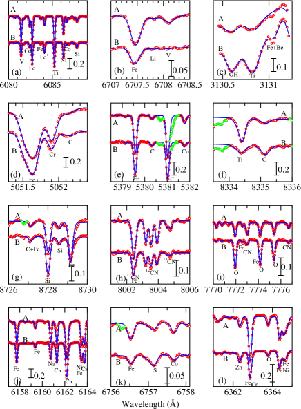
Fig. 5 : Synthetic spectrum fittings carried out (mainly) for determining the abundances of light elements.(cf. Table 3). The observed spectra are plotted in red symbols (where the masked regions discarded in judging the goodness of fit are colored in light-green) while the best-fit theoretical spectra are shown in blue solid lines. The wavelength scale is adjusted to the laboratory system. (a) 6080–6089 Å region, (b) 6707–6708.5 Å region, (c) 3130.45–3131.2 Å region, (d) 5051.3–5052.4 Å region, (e) 5378.5–5382 Å region, (f) 8333.5–8336 Å region, (g) 8726–8730 Å region, (h) 8001–8006 Å region, (i) 7770–7777 Å region, (j) 6157–6164 Å region, (k) 6756–6758.1 Å region, and (l) 6361–6365 Å region. Note that the telluric lines in the 8001–8006 Å region, 8333.5–8336 Å region, and 6361–6365 Å region were removed by dividing by the spectra of a rapid rotator. Likewise, the broad Ca i autoionization feature in the 6361–6365 Å region was planarized by regarding it as a pseudo-continuum.

4.4 Equivalent width analysis

As done in T08, we also carried out a differential analysis relative to the Sun for the other 19 elements (Al, Si, K, Ca, Sc, Ti, V, Cr, Mn, Co, Ni, Cu, Sr, Y, Zr, La, Ce, Pr, and Nd) based on the equivalent widths of usable spectral lines, which were measured directly from the OAO spectra by the Gaussian fitting method. The procedures of this analysis are detailed in Section 4.1 of Takeda et al. (2005). The solar equivalent widths used as the reference for this analysis were derived similarly by Gaussian-fitting technique on Kurucz et al.’s (1984) solar flux spectrum. The resulting [X/H] values (line-by-line abundances relative to the Sun) for $\gamma$ Leo A and B are presented in “ewanalys_A.dat” and “ewanalys_B.dat” of the online material, respectively.

It is worth noting that all these abundance results derived from equivalent widths are based on the conventional assumption that the line opacity is represented by a symmetric Voigt profile. However, lines of specific groups (e.g., Fe-peak elements of odd atomic number) are known to split into a number of sub-components (hyper-fine splitting), though the nature of splitting and its significance widely differs from case to case. In any event, care should be taken in interpreting the results obtained from such lines based on the single-line approximation. This effect is separately discussed for the representative cases of Sc, V, Mn, Co, and Cu lines in the Appendix.

4.5 Final abundances

Combining what has been described in Sect. 4.2–4.4, the final results of the differential abundances relative to the Sun for 26 elements (except for Li and Be, which are the special cases and thus separately treated in Sect. 5.1.1) derived for $\gamma$ Leo A and B are summarized in Table 7, where the differences between A and B ($\delta$[X/H]_A-B) are also given. The discussions presented in Sect. 5.1 and 5.2 will be primarily based on these data.

Table 7 : Elemental abundances of both components and their differences.

$Z$	Species	$T_{\rm c}$	Method	$N_{\rm A}$	[X/H]A	$\epsilon_{\rm A}$	$N_{\rm B}$	[X/H]B	$\epsilon_{\rm B}$	$\delta$[X/H]A-B
(1)	(2)	(3)	(4)	(5)	(6)	(7)	(8)	(9)	(10)	(11)
6	C i	40	fit	3	$-$0.62	0.07	3	$-$0.64	0.04	+0.02
7	N i	123	fit	1	$-$0.14	$\cdots$	1	$-$0.07	$\cdots$	$-$0.07
8	O i	180	fit	1	$-$0.33	$\cdots$	1	$-$0.33	$\cdots$	+0.00
11	Na i	958	fit	1	$-$0.24	$\cdots$	1	$-$0.37	$\cdots$	+0.13
13	Al i	1653	eqw	2	$-$0.21	0.02	2	$-$0.22	$\cdots$	+0.01
14	Si i	1310	eqw	33	$-$0.21	0.02	32	$-$0.25	0.02	+0.04
16	S i	664	fit	1	$-$0.36	$\cdots$	1	$-$0.45	$\cdots$	+0.09
19	K i	1006	eqw	1	$-$0.10	$\cdots$	1	$-$0.07	$\cdots$	$-$0.03
20	Ca i	1517	eqw	7	$-$0.31	0.02	6	$-$0.30	0.01	$-$0.01
21	Sc ii	1659	eqw	7	$-$0.32	0.03	8	$-$0.26	0.04	$-$0.06
22	Ti i	1582	eqw	35	$-$0.31	0.02	34	$-$0.32	0.02	+0.01
23	V i	1429	eqw	8	$-$0.32	0.02	8	$-$0.30	0.02	$-$0.02
24	Cr i	1296	eqw	18	$-$0.43	0.03	18	$-$0.39	0.02	$-$0.04
25	Mn i	1158	eqw	3	$-$0.42	0.06	3	$-$0.28	0.14	$-$0.14
26	Fe i	1334	eqw	191	$-$0.41	0.03	210	$-$0.38	0.02	$-$0.03
27	Co i	1352	eqw	8	$-$0.36	0.05	8	$-$0.33	0.03	$-$0.03
28	Ni i	1353	eqw	41	$-$0.41	0.02	42	$-$0.40	0.01	$-$0.01
29	Cu i	1037	eqw	1	$-$0.31	$\cdots$	1	$-$0.36	$\cdots$	+0.05
30	Zn i	726	fit	1	$-$0.22	$\cdots$	1	$-$0.31	$\cdots$	+0.09
38	Sr i	1464	eqw	1	$-$0.20	$\cdots$	1	$-$0.23	$\cdots$	+0.03
39	Y ii	1659	eqw	3	$-$0.40	0.07	3	$-$0.36	0.06	$-$0.04
40	Zr i	1741	eqw	1	$-$0.32	$\cdots$	1	$-$0.34	$\cdots$	+0.02
57	La ii	1578	eqw	1	$-$0.09	$\cdots$	1	$-$0.16	$\cdots$	+0.07
58	Ce ii	1478	eqw	4	$-$0.26	0.01	4	$-$0.21	0.04	$-$0.05
59	Pr ii	1582	eqw	2	$-$0.32	0.11	2	$-$0.33	0.03	+0.01
60	Nd ii	1602	eqw	5	$-$0.06	0.07	5	$-$0.12	0.06	+0.06

(1) Atomic number. (2) Element species. (3) Condensation temperature (in K) taken from Table 8 (50% $T_{\rm c}$) of Lodders (2003). (4) Method for deriving the abundance: “fit” $\cdots$ spectrum fitting analysis , “eqw” $\cdots$ use of measured equivalent widths. (5) Number of available lines (or features) of each species for A. (6) Final [X/H] value (averaged differential abundance of element X relative to the Sun; in dex) for A. (7) Mean error of [X/H] ($\epsilon\equiv\sigma/\sqrt{N}$) for A (in dex). (8) Number of available lines (or features) for B. (9) Final [X/H] value for B. (10) Mean error of [X/H] for B. (11) Differential abundance of A relative to B ($\equiv[{\rm X/H}]_{\rm A}-[{\rm X/H}]_{\rm B}$; in dex).

5 Discussion

5.1 Light element abundances in context of theoretical predictions

We first discuss the abundances of light elements, which are expected to have suffered more or less changes from the initial composition, because nuclear-processed products are dredged-up to the surface by evolution-induced mixing of red giants.

5.1.1 Li and Be

Regarding lithium, our fitting analysis in the Li i 6708 region resulted in converged solutions at $A_{\rm Li}$ = $-0.81$ (A) and $-0.36$ (B). However, these abundances must not be seriously taken because they both should be regarded rather as upper limits, since the corresponding equivalent widths (1.6 and 0.9 mÅ) are comparable to or lower than the detection-limit value of a few mÅ (cf. Appendix 2 of T17, where it was remarked that $A_{\rm Li}\lesssim 0$ is below the reliability limit). Actually, the Li i 6708 line feature is too weak to be recognizable by an eye(cf. Fig. 5b) What can be said about the surface lithium abundances of $\gamma$ Leo A and B is that they have suffered considerable depletion due to an efficient envelope mixing in the past (cf. Fig. 19 in T17 for reference).

As to beryllium, the abundance results are unfortunately less reliable, because the Be ii 3131 feature is seriously blended with the neighboring Fe line (owing to the appreciably large macroturbulence in this UV region presumably due to its height-increasing nature) and the Fe abundance had to be fixed (i.e. simultaneous determination with Be was not possible). Given this in mind, the derived $A_{\rm Be}$ values of $-0.23$ (A) and $0.08$ (B) correspond to [Be/Fe] = $-1.24$ (A) and $-0.96$ (B) (assuming $A_{\rm Be\odot}=1.42$ as in T14), which suggests that the Be deficiency is more or less compatible with the theoretical prediction expecting [Be/Fe] $\sim-1$ to $-2$ (see the orange line corresponding to $M=1.5M_{\odot}$ in Fig. 6 of T14).

5.1.2 C, N, O, and Na

The key elements, the abundances of which may be affected by the dredge-up of H-burning products are C, N, O (CNO-cycle), and Na (NeNa-cycle). The relative abundance ratios of [C/Fe], [N/Fe], [O/Fe], and [Na/Fe] for $\gamma$ Leo A/B are $-0.21/-0.26$, $+0.27/+0.31$, $+0.08/+0.05$, and $+0.17/+0.01$, respectively, The characteristics (almost similar for both A and B) are: (i) [C/Fe] is subsolar by $\sim$ 0.2–0.3 dex, (ii) [N/Fe] is supersolar by $\sim 0.3$ dex, (iii) [O/Fe] is slightly supersolar by $\lesssim 0.1$ dex, and [Na/Fe] is by $\lesssim 0.2$ dex supersolar (A) or almost solar (B). Likewise, an appreciably low ¹²C/¹³C ratio around $\sim 10$ was obtained for both stars.

These trends are more or less (at least qualitatively) consistent with the theoretical expectations (cf. Fig. 11 in T15 for C, O, and Na; Fig. 12 in T19 for N and ¹²C/¹³C). The slightly positive [O/Fe] (despite that O may suffer a very slight deficiency by $\lesssim$ a few hundredths dex; cf. Fig. 11b) is attributed to the chemical evolution effect for a mildly lower metallicity of [Fe/H] $\sim-0.4$. Accordingly, we may state that the abundance characteristics of these light elements are reasonably explained by the canonical theory of stellar evolution.

5.1.3 Comparison with previous work

Lambert & Ries’s (1981) pioneering study of CNO abundances for 32 G–K giants (based on [O i] lines and C₂ as well as CN molecular lines) included both $\gamma$ Leo A/$\gamma$ Leo B, for which they obtained $-0.26/-0.31$ for [C/Fe], $+0.42/+0.25$ for [N/Fe], $+0.17/+0.12$ for [O/Fe], and $6.5/9$ for ¹²C/¹³C. These values (along with the metallicities of [Fe/H] = $-0.35/-0.37$) are mostly consistent with our results, despite that the adopted lines are different.

However, a few previous studies done in 1990s reported apparently contradicting results regarding the C and N abundances. That is, a slightly subsolar [N/Fe] of $\sim-0.1$ and a somewhat supersolar [C/Fe] of $\sim+0.2$ were derived for $\gamma$ Leo A by Shavrina et al. (1996a) and Shavrina et al. (1996b) based on NH bands (around $\sim 3360$ Å) and CH bands (at 4230–4270 Å), which are just the opposite trend to what was obtained by Lambert & Ries (1981) and in this paper. Then, an independent study (again based on the NH bands around $\sim 3360$ Å) was soon after carried out by Yakovina & Pavlenko (1998), who concluded [N/Fe] = $0.0(\pm 0.1)$ for $\gamma$ Leo A (slightly higher by 0.1 dex than Shavrina et al.’s result). In any event, the C and N abundances of $\gamma$ Leo A derived by these groups from the spectrum-synthesis analysis of CH and NH bands in the blue–UV region are in conflict with the standard stellar evolution theory, which predicts a C-deficiency as well as an N-enrichment by a few tenths dex. Although any definite argument can not be made, their conclusions seem to be questionable. Since absolute CNO abundances determined from the molecular bands of hydride molecules (CH, NH, and OH) in short wavelength regions tend to suffer systematic errors, these errors for the target red giant and the Sun may not have been well cancelled out in the resulting differential abundances ([C/H] and [N/H]). Anyway, this problem is worth further investigation.

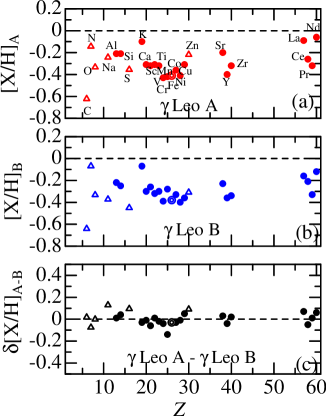
Fig. 6 : In panels (a) and (b) are plotted the [X/H] values (logarithmic abundance of element X relative to the Sun) against the atomic number ($Z$) for $\gamma$ Leo A and B, respectively. The differences between A and B ($\delta$[X/H]${}_{{\rm A}-{\rm B}}\equiv$ [X/H]${}_{\rm A}-$[X/H]_B) are also shown in the bottom panel (c). The results derived from the spectrum synthesis analysis are shown by triangles while those from the equivalent width analysis are by circles (the data points for Fe are depicted by double circles). Note that the results for Li and Be are not shown here.

5.2 Any abundance difference between A and B?

Searching for characteristic chemical signatures in stars specific to their planet-harboring nature (such as metal-rich tendency, abundance differences between volatile and refractory species; etc.) is important, since they may serve as a key to clarifying the physical mechanism of planet formation. A number of spectroscopic investigations on the chemical abundances of planet-host stars (along with the comparison sample of non-planet-host stars) have been done toward this aim over the past quarter century. Although solar-type stars (FGK-type dwarfs) have been primarily targeted in most of these studies, several recent papers have focused also on evolved red giants (retired A-type stars) reflecting the increasing number of planets discovered around giants; e.g., Maldonado, Villaver, & Eiroa (2013), da Silva et al. (2015), and Jofré et al. (2015), and Maldonado & Villaver (2016). While some possible characteristic trends specific to planet-host giants are reported compared to normal non-planet-host giants (e.g., possible metal-rich tendency in the higher-mass regime, small difference in [X/Fe] for some elements), they are generally subtle and indistinct. Moreover, it is not easy to discern the effect due to the existence of planets from the systematic problem caused by the difference between the samples.

In contrast, our approach is more straightforward and simple: To examine whether any difference exists in the elemental abundances between $\gamma$ Leo A (with planet) and $\gamma$ Leo B (without planet), both of which are considered to have formed from the gas with the same composition. Based on the results summarized in Table 7, the final abundances relative to the Sun for 26 elements from C to Nd ([X/H]_A, [X/H]_B, and their differences $\delta$[X/H]_A-B) are plotted against the atomic number in Fig. 6a–c. As seen from Table 7 and Fig. 6c, $|\delta$[X/H]${}_{{\rm A}-{\rm B}}|\lesssim 0.1$ dex holds for almost all of the studied elements.

The abundance errors due to ambiguities in atmospheric parameters ($T_{\rm eff}$, $\log g$, and $v_{\rm t}$) can be estimated for C, N, O, Na, S, and Zn (fitting-based abundances) by consulting Table 3 in T15, Table 3 in T16, and Table 2 in T19. Adopting $\pm 20$ K, $\pm 0.1$ dex, and $\pm 0.1$ km s^-1 for the uncertainties in $T_{\rm eff}$, $\log g$, and $v_{\rm t}$ (cf. Sect. 3.1), we obtained the corresponding abundance errors (root-sum-square of three error components) as $\pm 0.04$ dex for C i 5380 (though this line was eventually discarded, it is typical for high-excitation C i lines such as C i 5052 and C i 8335), $\pm 0.06$ dex for [C i] 8727, $\pm 0.04$ dex for N (from CN 8003), $\pm 0.06$ dex for O i 7774, $\pm 0.03$ dex for Na i 6161, $\pm 0.06$ dex for S i 6757, and $\pm 0.04$ dex for Zn i 6362. Meanwhile, regarding the abundances for many other elements derived from directly measured equivalent widths, their mean errors ($\epsilon$) given in Table 7 are mostly within $\lesssim$ 0.06–0.07 dex (exceptionally as large as $\sim 0.1$ dex for a few cases). We may thus regard that the errors involved in both [X/H]_A and [X/H]_B values are $\lesssim 0.1$ dex, which means that the abundances of $\gamma$ Leo A (with planet) and B (without planet) are practically the same (i.e., the $|\delta$[X/H]${}_{{\rm A}-{\rm B}}|$ values of $\lesssim 0.1$ dex are within the uncertain range). This conclusion may imply that the existence of a planet around A does not have any appreciable impact on the current surface chemical composition.

Our result is in agreement with the available previous work (cf. Table 1). Lambert & Ries’s (1981) CNO analysis for A and B resulted in almost the same similarity (cf. Sect. 5.1.3). Likewise, the same consequence can be drawn from the abundances of $\gamma$ Leo A and B derived by McWilliam (1990): Table 13 in his paper shows that the values of $\langle\delta A_{\rm{A}-\rm{B}}\rangle$ (mean differential abundances between A and B averaged over available lines) are +0.14, 0.00, +0.02, $-0.07$, +0.05, $-0.04$, $+0.04$, +0.06, $-0.06$, +0.06, +0.03, and +0.05 dex for Si i, Ca i, Sc ii, Ti i, Ti ii, V i, Co i, Ni i, Y ii, La ii, Nd ii, and Eu ii, respectively.

Finally, the [X/Fe] vs. $T_{\rm c}$ plots for A and B are also displayed in Fig. 7. Although this diagram is known to be useful in searching for any chemical signature of proto-planetary material accreted at the time of planet formation (i.e., abundance difference between volatile elements of low $T_{c}$ and refractory elements of high $T_{\rm c}$), its interpretation is difficult in the present case of red giants, because CNO abundances (representative low-$T_{\rm c}$ elements) tend to suffer changes due to an evolution-induced mixing. Anyway, no apparent $T_{\rm c}$-dependent trend is observed in [X/Fe] for both A and B (Fig. 7a and Fig. 7b)..

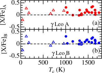
Fig. 7 : The [X/Fe] values ($\equiv[{\rm X/H}]-[{\rm Fe/H}]$; logarithmic X-to-Fe abundance ratios relative to the Sun) are plotted against $T_{\rm c}$ (condensation temperature). Panels (a) and (b) are for $\gamma$ Leo A and B, respectively. Otherwise, the same as in Fig. 6.

5.3 Mass-related problems

As summarized in Table 2, the mass values were derived in Sect. 3.2 as 1.66 $M_{\odot}$ (A) and 1.55 $M_{\odot}$ (B) from the positions on the HR diagram in comparison with theoretical evolutionary tracks. Since the corresponding $\log g_{MR}$ (1.80 and 2.56; evaluated from $M$ and $R$) are consistent with the spectroscopic $\log g$ (1.89 and 2.53) and the resulting $age$s for A and B are in agreement with each other at $\sim 2$ Gyr within the error bars (cf. Fig. 3), we may regard that these masses are reasonable.

As mentioned in Sect 1, previously determined mass values of $\gamma$ Leo A are considerably diversified from $\sim 1.2M_{\odot}$ to $\sim 1.8M_{\odot}$ (cf. Table 1). Especially, since the value of 1.23 $M_{\odot}$ adopted by Han et al. (2010) is presumably too low, the mass of the planet discovered by them ($m_{\rm p}\sin i_{\rm p}=8.78M_{\rm Jupiter}$) should be revised upward by a factor of $(1.66/1.23)^{2/3}$ as $m_{\rm p}\sin i_{\rm p}\simeq 10.7M_{\rm Jupiter}$. This value has got closer to the critical demarcation mass ($13M_{\rm Jupiter}$) between planet and brown dwarf, increasing a possibility that this substellar object orbiting around $\gamma$ Leo A may rather fall in the category of brown dwarf (depending on the inclination angle $i_{\rm p}$).

As already remarked in Sect. 1, the orbital elements of $\gamma$ Leo system are still subject to large uncertainties because of its very long period over several centuries. For example, according to Burnham’s Celestial Handbook (Burnham 1978), determinations of its orbital period in old literature are considerably diversified from $\sim 400$ yr to $\sim 700$ yr. The Sixth Catalog of Orbits of Visual Binary Stars (WDS-ORB6; cf. Hartkopf et al. 2001) gives $P=554(\pm 27)$ yr (period), $a=3.10(\pm 0.10)$ arcsec (semimajor axis), $i=41(\pm 5)^{\circ}$ (inclination angle), and $e=0.93(\pm 0.02)$ (ellipticity) for $\gamma$ Leo, though a low grade ‘4 (preliminary)’ is assigned to these data. Then, revised elements were published by Mason et al. (2006; cf. Table 7 therein), as $P=510.3$ yr, $a=4.24$ arcsec, $i=76.0^{\circ}$, and $e=0.845$ (again with grade ‘4’). Following Kepler’s third law, the sum of the masses in a binary system ($M_{\rm A}+M_{\rm B}$ in unit of $M_{\odot}$) is expressed in terms $a$ (in arcsec), $\pi$ (parallax; in arcsec), and $P$ (in yr) as $M_{\rm A}+M_{\rm B}=a^{3}\pi^{-3}P^{-2}$. However, this relation (with $\pi=25.07\times 10^{-3}$ arcsec) yields $M_{\rm A}+M_{\rm B}=6.2~{}M_{\odot}$ (in case of WDS-ORB6 elements) or $18.6M_{\odot}$ (in case of Mason et al.’s elements), which seriously disagree with our result of $M_{\rm A}+M_{\rm B}=3.21M_{\odot}$ obtained in this study. This discrepancy manifestly suggests that the published orbital elements of the $\gamma$ Leo system (even the latest ones) should be viewed with caution. Further long-running observations (at least over the next hundreds of years) would be required before this problem could be settled.

6 Summary and conclusion

$\gamma$ Leo is a binary system comprising two similar red giants of A (with planet) and B (without planet). It is worthwhile to examine if any difference exists between the surface abundances between these two, which may provide some information on a possible impact of planet formation upon the chemistry of the host star.

Yet, spectroscopic studies intending to clarify the chemical properties for both A and B seem to have been barely conducted so far. This motivated the author to newly determine the abundances of many elements for both components based on the high-dispersion spectra covering wide wavelength ranges.

Besides, the stellar parameters and related characteristics (e.g., stellar activity, kinematic information, etc.) were also studied because they are not necessarily well established, where particular attention was paid to clarifying the stellar mass (for which published results are diversified).

In addition, the nature of internal mixing in these evolved stars could be checked based on the light element abundances, because conflicting arguments were made by different authors regarding the surface abundances of C and N in $\gamma$ Leo A (i.e., whether or not they are well explained by the standard theory for the evolution-induced dredge-up of H-burning products).

The atmospheric parameters ($T_{\rm eff}$, $\log g$, and $v_{\rm t}$) were spectroscopically determined from Fe i and Fe ii lines. The resulting Fe abundances are [Fe/H] = $-0.41$ (A) and $-0.38$ (B); i.e., almost the same at a mildly subsolar metallicity. The kinematic parameters suggest that this system belongs to the thin-disk population.

The masses were derived from the positions on the HR diagram in comparison with theoretical evolutionary tracks as 1.66 $M_{\odot}$ (A) and 1.55 $M_{\odot}$ (B). Both A and B are likely to be in the stage of red clump giants after He-ignition. According to the newly determined $M_{\rm A}$, the mass of the planet around A was also revised as $m_{\rm p}\sin i_{\rm p}\simeq 10.7M_{\rm Jupiter}$ (increased by $\sim 20\%$ from the original value reported by Han et al.).

The chromospheric activity was estimated from the core emission strength of the Ca ii 3934 line, and the projected rotational velocity ($v_{\rm e}\sin i$) was determined from the spectrum-fitting analysis. It turned out that both $\gamma$ Leo A and B are typical red giant stars of low activity and low rotational velocities.

Chemical abundances of especially important elements (Li, Be, C, N, O, Na, S, and Zn; either being affected by evolution-induced mixing or volatile species) were determined by the spectrum-fitting technique. Meanwhile, those of the remaining elements (Al, Si, K, Ca, Sc, Ti, V, Cr, Mn, Co, Ni, Cu, Sr, Y, Zr, La, Ce, Pr, and Nd; mostly refractory species) were derived by the conventional method using the directly measured equivalent widths.

Regarding the mixing-affected light elements, although much can not be said about Li (very depleted; only upper limit) and Be (considerably deficient by $\sim-1$ dex, though less reliable) , a moderate deficiency of C, a mild enrichment of N, and a slight overabundance of Na, and a low ¹²C/¹³C ratio were obtained for both A and B, which are quite consistent with the trend expected from the canonical theory of stellar evolution. Likewise, the slightly positive [O/Fe] is reasonable for these somewhat metal-poor stars (galactic chemical evolution effect).

The chemical abundances of A and B turned out to be practically the same within $\lesssim 0.1$ dex for almost all elements, which implies that the surface chemistry is not appreciably affected by the existence of a planet in A. Likewise, any meaningful $T_{\rm c}$-dependent trend (or difference between volatile and refractory species) in [X/Fe] was not observed.

Accordingly, what can be concluded from this investigation is as follows.

• Based on the results summarized above, we may state that the visual binary system $\gamma$ Leo A+B is not so spectroscopically unusual as suspected initially when this investigation was motivated.

• The fact that no clear abundance difference was detected between A (with planet) and B (without planet) suggests that hosting a planet does not have an appreciable impact on the surface abundances of red giants, though this is an argument specific to $\gamma$ Leo and may not simply be generalized.

• The abundances of light elements are well consistent with those predicted from the canonical mixing theory of stellar evolution, which means that both $\gamma$ Leo A and B are ordinary red giants (presumably of red clump) like many others.

Data availability

The large data (equivalent widths, abundances, atomic data) of the spectroscopic analysis are given in the electronic data files of the supplementary material. The raw data for the spectra of $\gamma$ Leo A and B used in this investigation are in the public domain and available at https://smoka.nao.ac.jp/index.jsp (SMOKA Science Archive site).

Supplementary information

The following online data are available as supplementary materials accompanied with this article.

• readme.txt

• feabunds.dat

• ewanalys_A.dat

• ewanalys_B.dat

Statements and declarations

Funding

The author declares that no funds, grants, or other support were received during the preparation of this manuscript.

Competing interests

The author has no relevant financial or non-financial interests to disclose.

Author contributions

This investigation has been conducted solely by the author.

Appendix: Impact of hyperfine splitting on abundance determination

In the determination of the abundances for heavier elements based on the equivalent widths described in Sect. 4.4, the conventional single-line treatment was adopted where the line opacity is represented by a symmetric Voigt function. While this assumption is valid for most cases, lines of some elements (especially odd-$Z$ elements around $Z\sim$ 20–30) are known to intricately split into sub-components, which is caused by nucleus–electron coupling of the angular momentum. Since this effect (hyper-file splitting; abbreviated as “hfs”) acts as an extra broadening of the line opacity (while the total integrated opacity being kept unchanged) like the case of microturbulence, the equivalent width (of more or less saturated line) is increased by this splitting effect compared to the non-split case. As a result, the abundance derived from such a hfs-split line based on the usual single-component assumption tends to be overestimated unless the line is very weak.

The extents of overestimation caused by applying the single-component approximation were examined for the representative hfs lines of Sc ii ($Z=21$), V i ($Z=23$), Mn i ($Z=25$), Co i ($Z=27$), Cu i ($Z=29$). Out of the 29 lines for these 5 species analyzed in Sect. 4.4, 22 lines were selected for this test (cf. Table 8), for which the relevant hfs data (wavelengths and relative strengths of subcomponents) are available in the “gfhyperall.dat” file downloaded from the Dr. R. L. Kurucz’s web site.

By using the WIDTH9 program which was so modified as to enable incorporating the line-splitting effect by the spectrum-synthesis technique, two kinds of abundances [$A$(with hfs) and $A$(without hfs)] were obtained for given equivalent widths ($W_{\lambda}$), and the corresponding hfs corrections $\delta A[\equiv A$(with hfs)$-A$(without hfs)] were computed for $\gamma$ Leo A and B along with the Sun. Similarly, its effect on [X/H]_∗ (abundance of element X relative to the Sun) could be evaluated as $\delta$[X/H]${}_{*}\equiv\delta A_{*}-\delta A_{\odot}$. The results are summarized in Table 8, and in Fig. 8 are plotted these $\delta A$ as well as $\delta$[X/H] values against $W_{\lambda}$. An inspection of Fig. 8 reveals the following characteristics.

• The hfs corrections on the abundances ($\delta A$) are always negative, and $|\delta A|$ tends to be larger for stronger lines, as expected. However, their extents are considerably diversified from case to case depending on the detailed nature of line splitting. For example, even in the same strong-line regime ($W_{\lambda}\sim 100$ mÅ) for the case of $\gamma$ Leo A (Fig. 8a), $|\delta A|$ is almost negligible for Sc ii 5526.790 while significantly large ($\sim 0.3$ dex) for V i 5670.853.

• Roughly speaking, the inequality relation $|\delta A_{\odot}|<|\delta A_{\rm B}|<|\delta A_{\rm A}|$ holds for the relative importance of hfs corrections between $\gamma$ Leo A and B and the Sun (Fig. 8a and Fig. 8c). Therefore, as to $|\delta$[X/H]$|$ (generally smaller than $|\delta A|$ due to the subtraction of solar correction), $|\delta[{\rm X}/{\rm H}]_{\rm B}|$ is distinctly smaller than $|\delta[{\rm X}/{\rm H}]_{\rm A}|$. Actually, while $|\delta$[X/H]${}_{\rm A}|$ for $\gamma$ Leo A are still appreciable and significant (around $\sim 0.1$ dex on the average, though extending up to $\sim 0.3$ dex for some lines; cf. Fig. 8b), $|\delta$[X/H]${}_{\rm B}|$ for $\gamma$ Leo B is insignificant (confined within $\lesssim 0.05$ dex; cf. Fig. 8d).

• As seen from the different extent of hfs correction between the three cases (Sun $<$ $\gamma$ Leo B $<$ $\gamma$ Leo A), $T_{\rm eff}$ is presumably the most critical factor determining the significance of hfs, because it affects (i) the equivalent width of a line and (ii) the thermal width of line opacity, both affecting the degree of saturation. Accordingly, we may generally state that the impact of hfs on abundance determinations becomes more significant as $T_{\rm eff}$ is lowered.

Then, how much hfs correction should be applied to the relevant abundance results of Sc, V, Mn, Co, ad Cu obtained in Sect. 4.4 (which were derived from equivalent widths based on the single-line assumption neglecting hfs)? As long as the lines presented in Table 8 are concerned, while the corrections ($\delta$[X/H]_B) for $\gamma$ Leo B are apparently insignificant (only a few hundredths dex in any case), appreciable downward corrections ranging from $\sim 0.0$ to $\sim 0.3$ dex (considerably differing from line to line) are expected for $\gamma$ Leo A as seen from the values of $\delta$[X/H]_A. Fortunately, even in the latter case of $\gamma$ Leo A, since the lines of large corrections (by $\sim$ 0.2–0.3 dex) belong to the species (i.e., V or Co) using a sufficient number of lines (8–9), their impact tends to be mitigated after averaging. By applying the $\delta$[X/H] corrections of 22 lines (Table 8) to the [X/H] values obtained in Sect. 4.4 (cf. “ewanalys_A.dat” and “ewanalys_B.dat” in the online material), new mean $\langle$[X/H]$\rangle$ values (with hfs included) were calculated (where the same [X/H] data were used unchanged for the 7 lines for which hfs data were unavailable).

The resulting differences (in dex) of $\langle$[X/H]$\rangle$(with hfs)$-$$\langle$[X/H]$\rangle$(without hfs) are $-0.02|-0.02$ (Sc), $-0.07|0.00$ (V), $0.00|0.00$ (Mn), $-0.07|-0.02$ (Co), $-0.01|-0.01$ (Cu), for $\gamma$ Leo A$|$B, respectively. Accordingly, the hfs corrections on the final $\langle$[X/H]$\rangle$ results of Sc, V, Mn, Co, and Cu derived in Sect. 4.4 are only slight reductions by $\lesssim 0.1$ dex and thus not significant.

Table 8 : Hyperfine-splitting effect on the abundances of Sc, V, Mn, Co, and Cu.

Line	$W_{\lambda,\odot}$	$\delta A_{\odot}$	$W_{\lambda,{\rm A}}$	$\delta A_{\rm A}$	$\delta$[X/H]A	$W_{\lambda,{\rm B}}$	$\delta A_{\rm B}$	$\delta$[X/H]B
(1)	(2)	(3)	(4)	(5)	(6)	(7)	(8)	(9)
Sc ii 5318.349	14.0	$-$0.001	43.4	$-$0.004	$-$0.003	33.3	$-$0.003	$-$0.002
Sc ii 5526.790	75.6	$-$0.003	119.9	$-$0.001	+0.002	110.8	$-$0.003	0.000
Sc ii 5552.224	5.1	$-$0.001	22.8	$-$0.008	$-$0.007	16.9	$-$0.005	$-$0.004
Sc ii 5667.149	32.4	$-$0.026	76.7	$-$0.079	$-$0.053	63.9	$-$0.062	$-$0.036
Sc ii 5669.042	35.3	$-$0.002	86.6	$-$0.009	$-$0.007	76.9	$-$0.008	$-$0.006
Sc ii 5684.202	37.1	$-$0.028	86.4	$-$0.085	$-$0.057	74.6	$-$0.071	$-$0.043
Sc ii 6245.637	35.3	$-$0.027	83.9	$-$0.079	$-$0.052	71.6	$-$0.065	$-$0.038
V i 5657.435	6.5	$-$0.001	67.5	$-$0.048	$-$0.047	20.6	$-$0.008	$-$0.007
V i 5668.361	6.6	$-$0.005	67.0	$-$0.096	$-$0.091	21.7	$-$0.018	$-$0.013
V i 5670.853	19.7	$-$0.023	118.3	$-$0.290	$-$0.267	52.4	$-$0.071	$-$0.048
V i 6224.529	6.4	$-$0.015	91.4	$-$0.343	$-$0.328	25.9	$-$0.057	$-$0.042
V i 6266.307	3.3	$-$0.003	59.7	$-$0.094	$-$0.091	24.6	$-$0.031	$-$0.028
V i 6326.840	2.3	$-$0.004	26.8	$-$0.092	$-$0.088	7.8	$-$0.028	$-$0.024
V i 6531.415	6.9	$-$0.007	69.5	$-$0.100	$-$0.093	19.9	$-$0.016	$-$0.009
V i 7338.942	2.6	$-$0.010	20.0	$-$0.065	$-$0.055	6.9	$-$0.020	$-$0.010
Mn i 6440.971	6.4	$-$0.003	15.9	$-$0.008	$-$0.005	7.4	$-$0.003	0.000
Co i 5280.629	19.7	$-$0.090	53.0	$-$0.283	$-$0.193	32.7	$-$0.139	$-$0.049
Co i 5301.039	20.1	$-$0.019	93.3	$-$0.166	$-$0.147	55.3	$-$0.064	$-$0.045
Co i 5342.695	31.8	$-$0.146	59.1	$-$0.303	$-$0.157	43.7	$-$0.186	$-$0.040
Co i 5454.572	13.4	$-$0.042	27.7	$-$0.081	$-$0.039	19.3	$-$0.052	$-$0.010
Co i 6477.853	4.2	$-$0.013	16.0	$-$0.042	$-$0.029	8.7	$-$0.021	$-$0.008
Cu i 5218.197	52.7	$-$0.006	80.4	$-$0.017	$-$0.011	65.3	$-$0.014	$-$0.008

(1) Line designation. (2) Solar equivalent width (in mÅ). (3) Correction of the hyperfine-splitting effect to the solar abundance (in dex), which is defined as $\delta A\equiv A$(with hfs)$-A$(without hfs). (4) Equivalent width of $\gamma$ Leo A. (5) Hfs correction to the abundance of $\gamma$ Leo A. (6) Hfs correction to the [X/H] of $\gamma$ Leo A ($\equiv\delta A_{\rm A}-\delta A_{\odot}$). (7) Equivalent width of $\gamma$ Leo B. (8) Hfs correction to the abundance of $\gamma$ Leo B. (9) Hfs correction to the [X/H] of $\gamma$ Leo B.

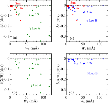
Fig. 8 : Corrections to the absolute ($A$) or relative ([X/H]) abundances due to the hyperfine-splitting effect (cf. Table 8) are plotted against the equivalent widths, where the open circles, filled circles, Greek crosses (+), half-filled triangles, and St. Andrew’s crosses ($\times$) correspond to Sc, V, Mn, Co, and Cu, respectively. (a) Hfs corrections to $A$ for $\gamma$ Leo A (green) and the Sun (red). (b) Hfs corrections to [X/H] for $\gamma$ Leo A. (c) Hfs corrections to $A$ for $\gamma$ Leo B (blue) and the Sun (red). (d) Hfs corrections to [X/H] for $\gamma$ Leo B.

References

- (1) Alonso, A., Arribas, S., & Martínez-Roger, C. 1999, Astron. Astrophys. Suppl. Ser., 140, 261
- (2) Bensby, T., Feltzing, S., Lundström, I., & Ilyin, I. 2005, Astron. Astrophys., 433, 185
- (3) Bressan, A., Marigo, P., Girardi, L., Salasnich, B., Dal Cero, C., Rubele, S., & Nanni, A. 2012, Mon. Not. R. Astron. Soc., 427, 127
- (4) Burnham, R. Jr. 1978, Burnham’s Celestial Handbook: An Observer’s Guide to the Universe Beyond the Solar System, Vol. II (Dover: New York), p.1063
- (5) Carlberg, J. K., Cunha, K., Smith, V. V., & Majewski, S. R. 2012, Astrophys. J., 757, 109
- (6) Cenarro, A. J., et al. 2007, Mon. Not. R. Astron. Soc., 374, 664
- (7) Charbonnel, C., et al. 2020, Astron. Astrophys., 633, A34
- (8) da Silva, L., et al. 2006, Astron. Astrophys., 458, 609
- (9) da Silva, R., Milone, A. de C., & Rocha-Pinto, H. J. 2015, Astron. Astrophys., 580, A24
- (10) Dyck, H. M., van Belle, G. T., & Thompson, R. P. 1998, Astron. J., 116, 981
- (11) Hakkila, J., Myers, J. M., Stidham, B. J., & Hartmann, D. H. 1997, Astron. J., 114, 2043
- (12) Han, I., Lee, B. C., Kim, K. M., Mkrtichian, D. E., Hatzes, A. P., & Valyavin, G. 2010, Astron. Astrophys., 509, A24
- (13) Hartkopf, W. I., Mason, B. D., & Worley, C. E. 2001, Astron. J., 122, 3472
- (14) Jofré, E., Petrucci, R., Saffe, C., Saker, L., Artur de la Villarmois, E., Chavero, C., Gómez, M., & Mauas, P. J. D. 2015, Astron. Astrophys., 574, A50
- (15) Jönsson, H., Ryde, N., Nordlander, T., Pehlivan Rhodin, A., Hartman, H., Jönsson, P., & Eriksson, K. 2017, Astron. Astrophys., 598, A100
- (16) Kovtyukh, V. V., Soubiran, C., Bienaymé, O., Mishenina, T. V., & Belik, S. I. 2006, Mon. Not. R. Astron. Soc., 371, 879
- (17) Kurucz, R. L. 1993, Kurucz CD-ROM No.13 (Cambridge: Smithsonian Astrophysical Observatory) [available at http://kurucz.harvard.edu/cdroms.html]
- (18) Kurucz, R. L., & Bell B. 1995, Kurucz CD-ROM, No. 23 (Cambridge: Smithsonian Astrophysical Observatory) [available at http://kurucz.harvard.edu/cdroms.html]
- (19) Kurucz, R. L., Furenlid, I., Brault, J., & Testerman, L. 1984, Solar Flux Atlas from 296 to 1300 nm (Sunspot, New Mexico: National Solar Observatory)
- (20) Lagarde, N., Decressin, T., Charbonnel, C., Eggenberger, P., Ekström, S., & Palacios, A. 2012, Astron. Astrophys., 543, A108
- (21) Lambert, D. L., & Ries, L. M. 1981, Astrophys. J., 248, 228
- (22) Lodders, K. 2003, Astrophys. J., 591, 1220
- (23) Lomaeva, M., Jönsson, H., Ryde, N., Schultheis, M., & Thorsbro, B. 2019, Astron. Astrophys., 625, A141
- (24) Maldonado, J., & Villaver, E. 2016, Astron. Astrophys., 588, A98
- (25) Maldonado, J., Villaver, E., & Eiroa, C. 2013, Astron. Astrophys., 554, A84
- (26) Mason, B. D., Hartkopf, W. I., Wycoff, G. L., & Holdenried, E. R. 2006, Astron. J., 132, 2219
- (27) Massarotti, A., Latham, D. W., Stefanik, R. P., & Fogel, J. 2008, Astron. J., 135, 209
- (28) McWilliam, A. 1990, Astrophys. J. Suppl. Ser., 74, 1075
- (29) Meléndez, J., Asplund, M., Gustafsson, B., & Yong, D. 2009, Astrophys. J., 704, L66
- (30) Primas, F., Duncan, D. K., Pinsonneault, M. H., Deliyannis, C. P., & Thorburn, J. A. 1997, Astrophys. J., 480, 784
- (31) Prugniel, Ph, Vauglin, I., & Koleva, M. 2011, Astron. Astrophys., 531, A165
- (32) Ryabchikova, T., Pakhomov, Yu, Mashonkina, L., & Sitnova, T. 2022, Mon. Not. R. Astron. Soc., 514, 4958
- (33) Ryabchikova, T., Piskunov, N., Kurucz, R. L., Stempels, H. C., Heiter, U., Pakhomov, Yu, & Barklem, P. S. 2015, Phys. Scr., 90, 054005
- (34) Sablowski, D. P., Järvinen, S., Ilyin, I., & Strassmeier, K. G. 2019, Astron. Astrophys., 622, L11
- (35) Santos, N. C., et al. 2013, Astron. Astrophys., 556, A150
- (36) Shavrina, A. V., Yakovina, L. A., & Bikmaef, I. F. 1996a, Kin. Phys. Cel. Bodies, Vol.12, No.1, p.35
- (37) Shavrina, A. V., Yakovina, L. A., & Boyarchuk, M. E. 1996b, Kin. Phys. Cel. Bodies, Vol.12, No.5, p.17
- (38) Smith, V. V., Lambert, D. L., & Nissen, P. E. 1998, Astrophys. J., 506, 405
- (39) Sousa, S. G., et al. 2015, Astron. Astrophys., 576, A94
- (40) Takeda, Y. 2007, Publ. Astron. Soc. Jpn., 59, 335
- (41) Takeda, Y. 2022, Astrophys. Space Sci., 367, 64
- (42) Takeda, Y., Kawanomoto, S., & Sadakane, K. 1998, Publ. Astron. Soc. Jpn., 50, 97
- (43) Takeda, Y., Ohkubo, M., & Sadakane, K. 2002, Publ. Astron. Soc. Jpn., 54, 451
- (44) Takeda, Y., Omiya, M., Harakawa, H., & Sato, B. 2016, Publ. Astron. Soc. Jpn., 68, 81 (T16)
- (45) Takeda, Y., Omiya, M., Harakawa, H., & Sato, B. 2019, Publ. Astron. Soc. Jpn., 71, 119 (T19)
- (46) Takeda, Y., Sato, B., Kambe, E., Izumiura, H., Masuda, S., & Ando, H. 2005, Publ. Astron. Soc. Jpn., 57, 109
- (47) Takeda, Y., Sato, B., & Murata, D. 2008, Publ. Astron. Soc. Jpn., 60, 781 (T08)
- (48) Takeda, Y., Sato, B., Omiya, M., & Harakawa, H. 2015, Publ. Astron. Soc. Jpn., 67, 24 (T15)
- (49) Takeda, Y., & Tajitsu, A. 2014, Publ. Astron. Soc. Jpn., 66, 91 (T14)
- (50) Takeda, Y., & Tajitsu, A. 2017, Publ. Astron. Soc. Jpn., 69, 74 (T17)
- (51) Takeda, Y., Tajitsu, A., Honda, S., Kawanomoto, S., Ando, H., & Sakurai, T. 2012, Publ. Astron. Soc. Jpn., 64, 130
- (52) Tomkin, J., Lambert, D. L., & Luck, R. E. 1975, Astrophys. J., 199, 436
- (53) Yakovina, L. A., & Pavlenko, Ya. V. 1998, Kin. Phys. Cel. Bodies, Vol.14, No.3, p.195