Asymptotic analysis of the characteristic polynomial for the Elliptic Ginibre Ensemble

Abstract.

We consider the Elliptic Ginibre Ensemble, a family of random matrix models interpolating between the Ginibre Ensemble and the Gaussian Unitary Ensemble and such that its empirical spectral measure converges to the uniform measure on an ellipse. We show the convergence in law of its normalised characteristic polynomial outside of this ellipse. Our proof contains two main steps. We first show the tightness of the normalised characteristic polynomial as a random holomorphic function using the link between the Elliptic Ginibre Ensemble and Hermite polynomials. This part relies on the uniform control of the Hermite kernel which is derived from the recent work of Akemann, Duits and Molag. In the second step, we identify the limiting object as the exponential of a Gaussian analytic function. The limit expression is derived from the convergence of traces of random matrices, based on an adaptation of techniques that were used to study fluctuations of Wigner and deterministic matrices by Male, Mingo, Péché and Speicher. This work answers the interpolation problem raised in the work of Bordenave, Chafaï and the second author of this paper for the integrable case of the Elliptic Ginibre Ensemble and is therefore a fist step towards the conjectured universality of this result.

1. Introduction and main result

1.1. The model of the Elliptic Ginibre Ensemble (EGE)

The random matrices that we consider in this paper are called Elliptic Ginibre Ensemble. This model is parameterized by $t\in[0,1]$ and interpolates between the Ginibre Ensemble and the Gaussian Unitary Ensemble (GUE) for $t=0$ and $t=1$ respectively. This ensemble has been studied extensively; see for instance [2], [22]. The generic law for any $t\in[0,1]$ is induced by the following construction.

Consider $X_{n}$ and $Y_{n}$ independent random matrices sampled from the Gaussian Unitary Ensemble of size $n\geq 1$. The law of the Elliptic Ginibre Ensemble at $t\in[0,1]$ is the law of the matrix

(1.1) $$A_{n,t}=\sqrt{\frac{1+t}{2}}X_{n}+i\sqrt{\frac{1-t}{2}}Y_{n},$$

where $i^{2}=-1$. Equivalently, the density of $A_{n,t}$ is proportional to the function, see [1, eq. (4)],

(1.2) $$\exp\left(-\frac{1}{1-t^{2}}\mathrm{Tr}\left[M^{*}M-\frac{t}{2}(M^{2}+(M^{*})^{2})\right]\right)\mathrm{d}M$$

where $\mathrm{d}M=\prod_{1\leq i,j\leq n}\mathrm{d}M_{i,j}$ is the product Lebesgue measure on the entries of the matrix. Many results are known for EGE matrices. In particular, the limiting eigenvalue distribution has been proved to be the uniform law on the ellipse centered at the origin with half long axis $1+t$ and short axis $1-t$. We refer to [16] and [34] for the study of this model.

In the recent work [12], it has been proved that the spectral radius of matrices with i.i.d coefficients, called Girko matrices, converges in probability to $1$ under the minimal assumption of a second moment on its entries. In order to derive this result, the authors considered the reciprocal characteristic polynomial associated to such matrices defined by $q_{n}(z)=z^{n}p_{n}\left(\frac{1}{z}\right)$ for $z\in\mathbb{D}$ where $p_{n}$ is the characteristic polynomial. The main result of [12] is the convergence in law, for the topology of local uniform convergence, of the sequence of functions $\{q_{n}\}_{n\geq 1}$ to a random function which is universal, in the sense that its expression involves only the second moment of the entries of the matrix. Our result aims at deriving the convergence of the normalised characteristic polynomial in the case of the EGE (1.1) at each $t\in[0,1]$ and at identifying the limiting object in the conjectured universality.
The same result holds for Haar unitary matrices, which is implied by the normal asymptotics of the traces of the powers of Haar unitary matrices [15] and by the asymptotics of the kernel which has a simple form in this case. Moreover, it can be even seen that the characteristic polynomial inside and outside exhibit the same but independent behavior. More interestingly, the scaling limit around a point at the unit circle has been studied in [13] by showing a convergence towards a random analytic function whose zeros form a determinantal point process on the real line.

1.2. Main result

Let $n\geq 1$ and $t\in[0,1]$. Consider $p_{n,t}(z)=\det(z-\frac{1}{\sqrt{n}}A_{n,t})$, the characteristic polynomial of a scaling by $\frac{1}{\sqrt{n}}$ of a matrix $A_{n,t}$ from the Elliptic Ginibre Ensemble (1.1). Define the normalised characteristic polynomial of $A_{n,t}$ by

$$f_{n,t}:\ \mathbb{D} \longrightarrow\mathbb{C}$$

(1.3) $$z \longmapsto\det\left(1+tz^{2}-\frac{z}{\sqrt{n}}A_{n,t}\right)\mathrm{e}^{-\frac{ntz^{2}}{2}}.$$

Our main result is the following convergence.

Theorem 1.1 (Convergence of the normalised characteristic polynomial for the EGE).

Let $t\in[0,1]$ and consider the sequence of random holomorphic functions $\{f_{n,t}\}_{n\geq 1}$ as in (1.3). Then, as $n\rightarrow\infty$,

$$f_{n,t}\xrightarrow[]{\mathrm{law}}f_{t}=\kappa_{t}\mathrm{e}^{-F_{t}}$$

for the topology of uniform convergence on compact subsets of $\mathbb{D}$, where the function $F_{t}$ is a Gaussian analytic function given by

(1.4) $$F_{t}(z)=\sum_{k\geq 1}X_{k,t}\frac{z^{k}}{\sqrt{k}}$$

for a family $(X_{k,t})_{k\geq 1}$ of independent complex Gaussian random variables such that $\mathbb{E}[X_{k,t}]=0$, $\mathbb{E}[X_{k,t}^{2}]=t^{k}$ and $\mathbb{E}[|X_{k,t}|^{2}]=1$, and the function $\kappa_{t}$ is given by

(1.5) $$\kappa_{t}(z)=\exp\left(-\frac{1}{2}\sum_{k\geq 1}\frac{h_{k,t}}{k}z^{2k}\right)\cdot\exp\left(\frac{tz^{2}}{2(1-tz^{2})}\right),$$

where the real coefficients $\{h_{k,t}\}_{k\geq 1}$ are given in (5.10).

Let us give some explanations on (1.3). In the case $t=0$, the matrix $A_{n,0}$ belongs to the Ginibre Ensemble, which is a particular case of Girko matrices. For such matrices, we have exactly the reciprocal characteristic polynomial of [12],

$$q_{n,0}:\ \mathbb{D}\longrightarrow\mathbb{C}$$

$$z\longmapsto q_{n,0}(z)=z^{n}p_{n,0}(g_{0}(z))$$

where $g_{0}:z\mapsto\frac{1}{z}$ is the conformal mapping that sends the unit disk to its complementary. One can think of the choice of $g_{0}$ as the following. We know that the empirical measure of eigenvalues of a Girko matrix converges weakly to the uniform measure on the unit disk $\mathbb{D}$, see [11] for complements on this universal result known as the circular law. One therefore chooses a mapping $g_{0}$ that sends $\mathbb{D}$ to the complementary of the support of the limiting eigenvalue measure so that $p_{n,0}\circ g_{0}$ does not vanish on the unit disk. Driven by this intuition, we construct $f_{n,t}$ by composing the characteristic polynomial by a function that sends $\mathbb{D}\setminus\{0\}$ to $\mathbb{C}\setminus E_{t}$ where $E_{t}$ is the support of the limiting eigenvalue distribution for the EGE with parameter $t$.

For $t\in[0,1]$, it has been proven in [34] that the average eigenvalue distribution for the Elliptic Ginibre Ensemble converges to the uniform distribution on the ellipsoid $E_{t}$ given by the equation

(1.6) $$E_{t}=\left\{x+iy\in\mathbb{C}:\left(\frac{x}{1+t}\right)^{2}+\left(\frac{y}{1-t}\right)^{2}\leq 1\right\}.$$

For $t=1$, we define $E_{1}$ to be the interval $[-2,2]$ and the corresponding limiting distribution to be the semi-circle distribution in accordance with Wigner’s theorem. Since the function $g_{t}:\ z\mapsto\frac{1}{z}+tz$ maps $\mathbb{D}\setminus\{0\}$ to $\mathbb{C}\setminus E_{t}$, a natural candidate for the normalised characteristic polynomial would be the mapping $z\mapsto z^{n}p_{n,t}\circ g_{t}(z)$. To have a convergence, it is necessary to add the factor $\exp\left(-\frac{ntz^{2}}{2}\right)$ which gives our expression of $f_{n,t}$ in (1.3). We refer the reader to Remark 5.13 for an explanation on this factor. Using these notations, from Theorem 1.1 we obtain the convergence of the normalised characteristic polynomial $\tilde{p}_{n,t}(u)=(g_{t}^{-1}(u))^{n}\mathrm{e}^{-nt(g_{t}^{-1}(u))^{2}/2}p_{n,t}(u)$

$$\tilde{p}_{n,t}\xrightarrow[]{\mathrm{law}}(\kappa_{t}\circ g_{t}^{-1})\mathrm{e}^{-F_{t}\circ g_{t}^{-1}}$$

in the topology of uniform convergence on compact sets of $\mathbb{C}\setminus E_{t}$. This is, in fact, equivalent to Theorem 1.1 due to the holomorphicity of $f_{n,t}$ at zero. It explains the notation “normalised characteristic polynomial” since $f_{n,t}$ and $\tilde{p}_{n,t}$ are the same functions in different coordinate systems.

From Theorem 1.1, one can derive the following result which was given in [30, Theorem 2.2] for a class of elliptic matrices that includes our Gaussian case. Nevertheless, since an explicit density can be written for the eigenvalues in the Gaussian case, we may also use large deviation arguments to obtain the lack of outliers.

Corollary 1.2 (Lack of outliers).

Let $C\subset\mathbb{C}$ be a closed set disjoint from $E_{t}$ and define $N_{n}(C)=\#\{i\in[n]:\frac{\lambda_{i}}{\sqrt{n}}\in C\}$. Then,

(1.7) $$N_{n}(C)\xrightarrow[]{\phantom{c}\mathbb{P}\phantom{c}}0.$$

Proof.

Let $C\subset\mathbb{C}$ be a closed set disjoint from $E_{t}$. Recall that $g_{t}(z)=\frac{1}{z}+tz$ and consider $\tilde{C}=g_{t}^{-1}(C)$ which is closed in $\mathbb{D}\setminus\{0\}$ so that its closure $K$ on $\mathbb{D}$ is compact. Then, we have that

$$\mathbb{P}[|N_{n}(C)|>0] =\mathbb{P}[\inf_{z\in C}|p_{n,t}(z)|=0]$$

$$=\mathbb{P}[\inf_{u\in K}|f_{n,t}(u)|=0]$$

$$\rightarrow\mathbb{P}[\inf_{u\in K}|f_{t}(u)|=0]=0.$$

∎

Figure 1. Illustration of Theorem 1.1. Phase portrait of the normalised characteristic polynomial of an EGE matrix of size $250$ for different values of $t$: 0 (top left), $0.3$ (top right), $0.6$ (bottom left) and $1$ (bottom right).

1.3. Method of proof

We will follow the same proof structure as for [12, Theorem 1.2], which was inspired by [9] and [18]. In order to prove the convergence in law for the topology of local uniform convergence, we will use [12, Lemma 3.2] which is close to [32, Proposition 2.5].

Lemma 1.3 (Tightness and convergence of coefficients imply convergence of functions).

Let $\{f_{n}\}_{n\geq 1}$ be a sequence of random elements in $\mathcal{H}(\mathbb{D})$ and denote the coefficients of $f_{n}$ by $(\xi_{k}^{(n)})_{k\geq 0}$ so that for all $z\in\mathbb{D}$, $f_{n}(z)=\sum_{k\geq 0}\xi_{k}^{(n)}z^{k}$. Suppose also that the following conditions hold.

• The sequence $\{f_{n}\}_{n\geq 1}$ is tight in $\mathcal{H}(\mathbb{D})$.

• For every $m\geq 0$, the vector $(\xi_{0}^{(n)},\dots,\xi_{m}^{(n)})$ converges in law as $n\to\infty$ to $(\xi_{0},\dots,\xi_{m})$ for a common sequence of random variables $(\xi_{k})_{k\geq 0}$.

Then, $f(z)=\sum_{k\geq 0}\xi_{k}z^{k}$ is a well-defined function in $\mathcal{H}(\mathbb{D})$ and $f_{n}$ converges in law towards $f$ in $\mathcal{H}(\mathbb{D})$ for the topology of local uniform convergence.

The first part of our proof of Theorem 1.1 is to show, for every fixed value of $t\in[0,1]$, the tightness (a) of the family of random functions $\{f_{n,t}\}_{n\geq 1}$. To do so, we will use the known properties of the Elliptic Ginibre Ensemble and its relation to scaled Hermite polynomials. A local uniform control is derived from the recent work [1]. This local uniform control allows us to derive tightness thanks to Lemma 2.2 below.

The second part of the proof consists in proving a convergence in distribution of the coefficients appearing in the functions $\{f_{n,t}\}_{n\geq 1}$. We reduce the former to proving convergence of traces of polynomials in $A_{n,t}$, which is classic in random matrix theory and is done by a combinatorial argument using the method of moments. The study we conduct will follow the lines developed in [23] in which the authors studied the asymptotic fluctuations of Wigner and deterministic matrices. As in [23], we will not use the Gaussian nature of $A_{n,t}$ but only the fact that all its moments are finite.
The use of the method of moments to derive a CLT for traces of random matrices was initiated by the work [21] in the context of Gaussian Wishart matrices. Using similar techniques, the authors in [33] derived a CLT for traces of Wigner matrices, together with a universality result on the limiting Gaussian distribution. Another approach leading to CLT for traces of random matrices is the resolvent method. For instance, one is able to prove CLT for functions that are analytic inside the support of the limiting eigenvalue distribution. We refer the reader to [8] for the case of Wigner matrices and [7] for Wishart matrices for a use of these techniques. For a more complete review on techniques leading to CLT, see also the introduction of [5] and references therein.

Finally, since the way we show tightness is by controlling the second moment of $f_{n,t}$ and since this second moment depends only on the first four moments of $A_{n,t}$, tightness of $f_{n,t}$ still holds for the model described in Subsection 1.4.1 for coefficients $(a_{ij})_{i,j\geq 1}$ whose first four moments coincide with those of the EGE. Moreover, the method of moments proof of the convergence of traces can be adapted to the case where the coefficients have all moments finite and Theorem 1.1 holds for coefficients $(a_{ij})_{i,j\geq 1}$ with all moments finite and whose first four moments coincide with those of the EGE.

1.4. Open questions and comments

1.4.1. Minimal moment condition and universality

As conjectured in [12], the convergence in Theorem 1.1 of the normalised characteristic polynomial is believed to hold under the minimal moment condition

(1.8) $$\mathbb{E}\left[|a_{1,2}|^{2}|a_{2,1}|^{2}\right]<\infty$$

on the entries $(a_{i,j})_{i,j\geq 1}$, which gives a condition of a fourth order moment for Wigner matrices and second order moment for Girko matrices. The more general context of condition (1.8) seems adapted to the model of elliptic random matrices. This model was introduced by Girko in [16] and [17]. A version of this consists of matrices having the following dependence relations be found in [28, Definition 1.3]. Fix some random vector $(\xi_{1},\xi_{2})$ in $\mathbb{C}^{2}$ with zero mean such that $\mathbb{E}[|\xi_{1}|^{2}]=\mathbb{E}[|\xi_{2}|^{2}]=1$. A matrix $A_{n}=(a_{i,j})_{1\leq i,j\leq n}$ is said to be elliptic with atom distribution $(\xi_{1},\xi_{2})$ if

• $(a_{i,i},1\leq i),\ ((a_{i,j},a_{j,i}),1\leq i<j)$ are independent families.

• $((a_{i,j},a_{j,i}),1\leq i<j)$ consists of i.i.d copies of $(\xi_{1},\xi_{2})$.

• $(a_{i,i},1\leq i)$ are i.i.d with zero mean and finite variance.

Convergence of the average eigenvalue distribution towards the uniform distribution on a rotated version of the ellipse (1.6) where $t=|\mathbb{E}[\xi_{1}\xi_{2}]|$ has been proved, under different conditions on the variables, in [28, 30, 27]. We expect a version of Theorem 1.1 to hold for the general elliptic matrices described above. This is work in progress.

1.4.2. Matrices with entries in $\{0,1\}$

In the recent work [14], a convergence of the reciprocal characteristic polynomial for matrices with independent Bernoulli entries with non-zero expectation has been proved. The limiting random function can be expressed using Poisson random variables, see [14, Theorem 2.3]. One could ask for an analogue of the Elliptic Ginibre Ensemble for such matrices and the convergence of its normalised characteristic polynomial.

1.4.3. Fluctuations of the extreme eigenvalue

For both Ginibre and GUE cases, one knows the law of the fluctuations of the largest eigenvalue around its limit. For the Ginibre Ensemble, one has Gumbel fluctuations for the maximum modulus around $1$, see [31], whereas for the GUE, one has Tracy-Widom fluctuations for the maximum eigenvalue around $2$, see [36] and references therein. In [19], we may find a family of determinantal processes that interpolates between a Poisson process with intensity $\mathrm{e}^{-x}$ and the Airy process. The distribution function of its last particle interpolates between the Gumbel and Tracy-Widom distributions, see [19, Theorem 1.3]. As a two-dimensional version, [10] considered the Elliptic Ginibre Ensemble and an interpolating determinantal processes to prove scaling limits for the eigenvalue point process.

1.4.4. Determinantal Coulomb gases

As explained in 1.4.1, this work can be thought of as a first step towards the convergence of the characteristic polynomial outside the support of the equilibrium measure for general elliptic random matrices. Nevertheless, we could have followed a different path, which is to look the Elliptic Ginibre Ensembles as a particular case of a determinantal Coulomb gas. In this vein, it may be possible to show the convergence of the traces by adapting results from [4] and to show tightness of the characteristic polynomial outside the support of the equilibrium measure for more general determinantal Coulomb gases by using, for instance, the results from [3].

2. Tightness of the normalised characteristic polynomial

This section is devoted to the proof of the following theorem.

Theorem 2.1 (Tightness).

For every $t\in[0,1]$, the sequence $\{f_{n,t}\}_{n\geq 1}$ is tight, viewed as random elements of $\mathcal{H}(\mathbb{D})$, the set of holomorphic functions on $\mathbb{D}$.

Since the case $t=0$ is treated in [12], we will assume for the rest of this section that $t\in(0,1]$.

Recall that for $z\in\mathbb{D}$, $n\geq 1$ and $t\in[0,1]$,

$$f_{n,t}(z)=\det\Big{(}1+tz^{2}-\frac{z}{\sqrt{n}}A_{n,t}\Big{)}\mathrm{e}^{-\frac{ntz^{2}}{2}}.$$

For our purposes, we will only be interested in the holomorphic function $f_{n,t}$ from $\mathbb{D}$ to $\mathbb{C}$. Equip the set $\mathcal{H}(\mathbb{D})$ with the topology of uniform convergence on compact sets. Lemma 2.2 below reduces the proof of tightness to a uniform control on compact subsets of $\mathbb{D}$.

Lemma 2.2 (Reduction to uniform control).

Fix $t\in[0,1]$. Suppose that for every compact $K\subset\mathbb{D}$, the sequence $(||f_{n,t}||_{K})_{n\geq 1}$ is tight, where $||f_{n,t}||_{K}=\max_{z\in K}|f_{n,t}(z)|$. Then, $\{f_{n,t}\}_{n\geq 1}$ is tight.

Proof.

It is a consequence of Montel’s theorem. See, for instance, [32, Proposition 2.5]. ∎

Remark 2.3.

By the subharmonicity of $|f_{n,t}(z)|^{2}$, saying that $\{\mathbb{E}[\|f_{n,t}\|_{K}^{2}]\}_{n\geq 1}$ is a bounded sequence for every compact $K\subset\mathbb{D}$ is equivalent to say that $\{\sup_{z\in K}\mathbb{E}[|f_{n,t}(z)|^{2}]\}_{n\geq 1}$ is a bounded sequence for every compact $K\subset\mathbb{D}$. See, for instance, [32, Lemma 2.6]. In the Girko case of [12], one had a remarkable orthogonality of the sub-determinants which led to an upper bound on the desired quantity. As we no longer have this property, our proof is based on the article [2], which exploits the integrability of the Elliptic Ginibre Ensemble.

The main result of this subsection is Proposition 2.7, proved in Section 4.3. Its proof is based on Lemma 2.5 below which expresses the quantity $\mathbb{E}[|f_{n,t}(z)|^{2}]$ in terms of Hermite polynomials. This lemma is proved in Section 4.1.

Definition 2.4 (Hermite polynomials).

The Hermite polynomials $\{He_{n}\}_{n\geq 0}$ are the monic orthogonal polynomials with respect to the measure $\mathrm{e}^{-x^{2}/2}\mathrm{d}x$ on $\mathbb{R}$ so that

$$\int_{\mathbb{R}}He_{n}(x)He_{m}(x)\mathrm{e}^{-\frac{x^{2}}{2}}\mathrm{d}x=\sqrt{2\pi}n!\delta_{n,m}.$$

Recall that for $t\in[0,1]$ and $z\neq 0$, we have $g_{t}(z)=z^{-1}+tz$.

Lemma 2.5 (Hermite expression of the characteristic polynomial).

For $n\geq 1$, $t\in(0,1]$ and $z\in\mathbb{D}\setminus\{0\}$, one has the following expression

(2.1) $$\mathbb{E}[|f_{n,t}(z)|^{2}]=\frac{n!|z|^{2n}}{n^{n}}\left|\mathrm{e}^{-ntz^{2}}\right|\sum_{k=0}^{n}\frac{t^{k}}{k!}\left|He_{k}\left(\sqrt{\frac{n}{t}}g_{t}(z)\right)\right|^{2}.$$

With the help of the expression (2.1) and using the results from [1], we will control $\mathbb{E}[|f_{n,t}(z)|^{2}]$ uniformly on bounded sets from above and from below. In fact, [1] allows us to give an explicit expression for the limit of $\mathbb{E}[|f_{n,t}(z)|^{2}]$ but since we do not need it, we will only state the following.

Lemma 2.6 (Convergence of the second moment).

Fix $t\in(0,1]$. There exists a continuous function $\mathcal{F}:\mathbb{D}\setminus\{0\}\to(0,\infty)$ such that, uniformly on compact sets,

$$\mathbb{E}[|f_{n,t}|^{2}]\xrightarrow[n\to\infty]{}\mathcal{F}.$$

But, since $f_{n,t}$ is holomorphic on the whole disk $\mathbb{D}$, the origin was never actually an issue so that one can extend the control on any $\mathbb{D}_{r}$ for $r\in(0,1)$. This is written in the next proposition.

Proposition 2.7 (Uniform control).

Fix $t\in(0,1]$. Then, for every $r\in(0,1)$ there exists $C_{r}>0$ such that, for every $n\geq 1$,

$$\mathbb{E}[\|f_{n,t}\|_{D_{r}}^{2}]\leq C_{r}.$$

Proposition 2.7 proves Theorem 2.1 thanks to Lemma 2.2 and Remark 2.3. The proof of the tightness $(a)$ in Lemma 1.3 is thus complete.

3. Convergence of the coefficients

In this section, we will prove the (b) part of Lemma 1.3. We thus have to study the convergence in law of the coefficients appearing in $f_{n,t}$. We will give a new expression of these coefficients, using a family of polynomials that we call the modified Chebyshev polynomials introduced in Definition 3.1.

Definition 3.1 (Modified Chebyshev polynomials).

For $t\in[0,1]$, the modified Chebyshev polynomials are the polynomials $\left\{P^{(t)}_{k}\right\}_{k\geq 0}$ satisfying the recurrence relation

(3.1) $$P_{k+1}^{(t)}=XP_{k}^{(t)}-tP^{(t)}_{k-1},\ \ P_{0}^{(t)}=2,\ \ P_{1}^{(t)}=X.$$

One has an alternative expression for $f_{n,t}$ given by the following proposition, proved in Section 5.1.

Proposition 3.2 (Trace expression).

For all $n\geq 1$, $t\in[0,1]$ and $z\in\mathbb{D}$ close to the origin,

(3.2) $$f_{n,t}(z)=\exp\left(-\sum_{k\geq 1}U_{k,t}^{(n)}\frac{z^{k}}{k}\right),$$

where

(3.3) $$U_{k,t}^{(n)}=\mathrm{Tr}\left[P_{k}^{(t)}\left(\frac{A_{n,t}}{\sqrt{n}}\right)\right]+nt\delta_{k=2}.$$

By Proposition 3.2, the coefficients $(\xi^{(n)}_{0,t},\dots,\xi^{(n)}_{m,t})$ of Lemma 1.3 (b) associated to $f_{n,t}$ can be expressed as polynomials (which do not depend on $n$) of coefficients $(U_{0,t}^{(n)},\dots,U_{m,t}^{(n)})$ and vice versa. Thus, showing the convergence in law of $\big{\{}\xi^{(n)}_{k,t}\big{\}}_{k}$ is equivalent to showing the convergence in law of $\big{\{}U_{k,t}^{(n)}\big{\}}_{k}$.

Since it is easier to deal with traces, we will study $U_{k,t}^{(n)}$. This is done in two steps, we study the convergence of the expectation in Lemma 3.3 and the convergence of fluctuations in Proposition 3.4 below. These statements are proved in Sections 5.3 and 5.4 respectively.

Lemma 3.3 (Convergence of the expectation).

For all $k\geq 1$, denote $e_{k,t}^{(n)}=\mathbb{E}\left[U_{k,t}^{(n)}\right]$. Then,

(3.4) $$e_{2k,t}^{(n)} =-kt^{k}+h_{k,t}+O\left(\frac{1}{n}\right)$$

(3.5) $$e_{2k+1,t}^{(n)} =o(1)$$

as $n\rightarrow\infty$. The explicit expression of $h_{k,t}$ can be found in (5.10).

Proposition 5.4 below shows that the variables $\left\{V_{k,t}^{(n)}=U_{k,t}^{(n)}-\mathbb{E}\left[U_{k,t}^{(n)}\right]\right\}_{k\geq 0}$ converge in law to a Gaussian family.

Proposition 3.4 (Convergence of the fluctuations).

For every $t\in[0,1]$, the family $\big{\{}V_{k,t}^{(n)}\big{\}}_{k\geq 0}$ converges in law to a family $\{V_{k,t}\}_{k\geq 0}$ of centered and independent complex Gaussians such that $\mathbb{E}[V_{k,t}^{2}]=kt^{k}$ and $\mathbb{E}[|V_{k,t}|^{2}]=k$.

Proposition 3.4 together with Lemma 3.3 show the convergence in distribution of $\left(U_{0,t}^{(n)},\dots,U_{m,t}^{(n)}\right)$ to $\left(V_{0,t},\dots,V_{m,t}\right)+(e_{0,t}^{(\infty)},\dots,e_{m,t}^{(\infty)})$ where $e_{2k,t}^{(\infty)}=-kt^{k}+h_{k,t}$ and $e_{2k+1,t}^{(\infty)}=0$ for $k\geq 1$. By Lemma 1.3, the limit of $f_{n,t}$ is the well-defined function $f_{t}\in\mathcal{H}(\mathbb{D})$ given, for $z$ small, by

(3.6) $$f_{t}(z)=\exp\left(-\sum_{k\geq 1}V_{k,t}\frac{z^{k}}{k}\right)\exp\left(-\sum_{k\geq 1}e_{k,t}^{(\infty)}\frac{z^{k}}{k}\right)=\kappa_{t}(z)\mathrm{e}^{-F_{t}(z)},$$

where

(3.7) $$F_{t}(z) =\sum_{k\geq 1}V_{k,t}\frac{z^{k}}{k}\quad\mbox{and}$$

(3.8) $$\kappa_{t}(z) =\exp\left(-\frac{1}{2}\sum_{k\geq 1}h_{k,t}\frac{z^{2k}}{k}\right)\cdot\exp\left(\frac{tz^{2}}{2(1-tz^{2})}\right)$$

which is the limit function in Theorem 1.1 with $X_{k,t}=\frac{1}{\sqrt{k}}V_{k,t}$. The series for $F_{t}$ defines a holomorphic function on the whole disk but it may not be clear that $\sum_{k\geq 1}e_{k,t}^{(\infty)}\frac{z^{k}}{k}$ also does. Since $f_{t}(0)=1$, we may take a holomorphic logarithm and notice that $\sum_{k\geq 1}e_{k,t}^{(\infty)}\frac{z^{k}}{k}$ converges for $z$ small, but we may have a problem for $z$ far from the origin. Nevertheless, $\kappa_{t}$ is well defined as $f_{t}e^{F_{t}}$ and it is deterministic on $\mathbb{D}$ since we have the deterministic expression near the origin given by (3.8). To show that $\sum_{k\geq 1}e_{k,t}^{(\infty)}\frac{z^{k}}{k}$ converges for $z\in\mathbb{D}$, it would be enough to show that $f_{t}e^{F_{t}}$ has no zeros since, in that case, we can take a holomorphic logarithm of $f_{t}e^{F_{t}}$ which would coincide, up to an additive constant, with $\sum_{k\geq 1}e_{k,t}^{(\infty)}\frac{z^{k}}{k}$ near the origin. That $\kappa_{t}=f_{t}e^{F_{t}}$ has no zeros can be seen by using Lemma 2.6 which implies that

$$0<\mathbb{E}[|f_{t}(z)|^{2}]=|\kappa_{t}(z)|^{2}\mathbb{E}[|e^{-F_{t}(z)}|^{2}]$$

for $z\in\mathbb{D}\setminus\{0\}$.

4. Proofs of statements used for tightness

4.1. Proof of Lemma 2.5

In the case of the Elliptic Ginibre Ensemble given by (1.1), the matrix $A_{n,t}$ has the following density, which can be found in [1, eq. (4)].

(4.1) $$\mathrm{d}\mathbb{P}_{t}(M)=\left(\frac{1}{\pi\sqrt{1-t^{2}}}\right)^{n^{2}}\exp\left(-\frac{1}{1-t^{2}}\mathrm{Tr}\left[MM^{*}-\frac{t}{2}(M^{2}+(M^{*})^{2})\right]\right)\mathrm{d}M$$

which has the form $\mathrm{d}\mathbb{P}_{t}(M)=w_{t}(M,M^{*})\mathrm{d}M$ associated to the weight function

$$w_{t}(z)=\frac{1}{\pi\sqrt{1-t^{2}}}\exp{\left(-\frac{1}{1-t^{2}}\left(|z|^{2}-\frac{t}{2}(z^{2}+\overline{z}^{2})\right)\right)}=\frac{1}{\pi\sqrt{1-t^{2}}}\exp{\left(-\left(\frac{x^{2}}{1+t}+\frac{y^{2}}{1-t}\right)\right)}$$

with $x=\mathrm{Re}(z)$ and $y=\mathrm{Im}(z)$. In order to use the main theorem of [2], we should compute the orthonormal polynomials with respect to $w_{t}(z)\mathrm{d}z$. Using results in [1, eq. (3)], these polynomials are $\{P_{n}\}_{n\geq 0}$ given by

(4.2) $$P_{n}(z)=\frac{\sqrt{t^{n}}}{\sqrt{n!}}He_{n}\left(\frac{z}{\sqrt{t}}\right).$$

Define $R_{n}(z)=\sqrt{t^{n}}He_{n}\left(\frac{z}{\sqrt{t}}\right)$ and $c_{n}=n!$. The family $\{R_{n}\}_{n\geq 0}$ are the monic orthogonal polynomials with respect to $w_{t}(z)\mathrm{d}z$. Using results of [2], one has for $M$ sampled from (4.1) and $u,v\in\mathbb{C}$, one has

(4.3) $$\mathbb{E}\left[\det(u-M)\overline{\det(v-M)}\right]=c_{N}\sum_{k=0}^{N}P_{k}(u)\overline{P_{k}(v)}.$$

Since $f_{n,t}(z)=\mathrm{e}^{-\frac{ntz^{2}}{2}}\left(\frac{z}{\sqrt{n}}\right)^{n}\det\left(\sqrt{n}(z^{-1}+tz)-A_{n,t}\right)$, setting $u=v=g_{t}(z)=\sqrt{n}(z^{-1}+tz)$ gives

$$\mathbb{E}|f_{n,t}(z)|^{2}=\frac{n!|z|^{2n}}{n^{n}}\left|\mathrm{e}^{-ntz^{2}}\right|\sum_{k=0}^{n}\frac{t^{k}}{k!}\left|He_{k}\left(\sqrt{\frac{n}{t}}g_{t}(z)\right)\right|^{2}$$

which is the desired expression of $\mathbb{E}|f_{n,t}(z)|^{2}$ in terms of Hermite polynomials.

4.2. Proof of Lemma 2.6

Recall the function $g_{t}:\mathbb{D}\to\mathbb{C}\setminus E_{t}$ given by $g_{t}(z)=\frac{1}{z}+tz$ and define $L_{n}:\mathbb{C}\setminus E_{t}\to[0,\infty)$ by

$$L_{n}(u)=\sum_{k=0}^{n-1}\frac{t^{k}}{k!}\left|\mathrm{He}_{k}\left(\sqrt{\frac{n}{t}}u\right)\right|^{2}.$$

By using the contour integral representation around a small loop enclosing the origin,

$$L_{n}(u)=\frac{1}{2\pi i}\oint\displaylimits_{0}\frac{\mathrm{e}^{nF_{u}(s)}}{t-s}\frac{\mathrm{d}s}{\sqrt{1-s^{2}}},\quad\mbox{ with }\quad F_{u}(s)=\frac{s}{t}\left(\frac{\mathrm{Re}(z)^{2}}{1+s}+\frac{\mathrm{Im}(z)^{2}}{1-s}\right)-\log s+\log t,$$

the following has been proved in [1, Theorem II.12, (i)] and [1, Theorem II.13, (i)] in the case $t=1$ for $u\in\mathbb{C}\setminus E_{t}$ and $z=g_{t}^{-1}(u)$,

(4.4) $$L_{n}(u)=\frac{1}{2\pi}\sqrt{\frac{2\pi}{nF_{u}^{\prime\prime}(t|z|^{2})}}\frac{\mathrm{e}^{nF_{u}(t|z|^{2})}}{\sqrt{1-t^{2}|z|^{4}}}\frac{1}{t(1-|z|^{2})}\left(1+O\left(\frac{1}{n}\right)\right),$$

where the error term is uniform on compact sets of $\mathbb{C}\setminus E_{t}$. In our case we need to control

$$\mathbb{E}[|f_{n,t}(z)|^{2}] =\frac{n!|z|^{2n}}{n^{n}}\mathrm{e}^{-nt\mathrm{Re}(z^{2})}\sum_{k=0}^{n}\frac{t^{k}}{k!}\left|\mathrm{He}_{k}\left(\sqrt{\frac{n}{t}}\left(\frac{1}{z}+tz\right)\right)\right|^{2}$$

$$=\frac{n!|z|^{2n}}{n^{n}}\mathrm{e}^{-nt\mathrm{Re}(z^{2})}L_{n+1}\left(\sqrt{\frac{n}{n+1}}g_{t}(z)\right).$$

The term $F_{u}(t|z|^{2})$ in (4.4) can be explicitly calculated by using [1, eq. (32)] or, in a more direct way,

$$F_{u}(t|z|^{2}) =|z|^{2}\left(\frac{\mathrm{Re}\left(\frac{1}{z}+tz\right)^{2}}{1+t|z|^{2}}+\frac{\mathrm{Im}\left(\frac{1}{z}+tz\right)^{2}}{1-t|z|^{2}}\right)-\log(t|z|^{2})+\log t$$

$$=|z|^{2}\left(\frac{\mathrm{Re}\left(\frac{1}{z}+t\bar{z}\right)^{2}}{1+t|z|^{2}}+\frac{\mathrm{Im}\left(\frac{1}{z}-t\bar{z}\right)^{2}}{1-t|z|^{2}}\right)-\log(|z|^{2})$$

$$=|z|^{2}\Big{(}\left(1+t|z|^{2}\right)\mathrm{Re}(1/z)^{2}+\left(1-t|z|^{2}\right)\mathrm{Im}(1/z)^{2}\Big{)}-\log(|z|^{2})$$

$$=1+t(z\bar{z})^{2}\mathrm{Re}(1/z)^{2}-t(z\bar{z})^{2}\mathrm{Im}(1/z)^{2}-\log(|z|^{2})$$

$$=1+t\mathrm{Re}(\bar{z})^{2}-t\mathrm{Im}(\bar{z})^{2}-\log(|z|^{2})$$

$$=1+t\mathrm{Re}(z^{2})-\log(|z|^{2}).$$

By (4.4) and Stirling’s formula, we immediately notice that

$$\frac{n!|z|^{2n}}{n^{n}}\mathrm{e}^{-nt\mathrm{Re}(z^{2})}L_{n}(g_{t}(z))$$

converges uniformly on compact sets of $\mathbb{D}\setminus\{0\}$ towards

$$\frac{1}{\sqrt{2\pi F_{u}^{\prime\prime}(t|z|^{2})(1-t^{2}|z|^{4})}t(1-|z|^{2})}.$$

It is now enough to notice that

$$\frac{L_{n+1}\left(\sqrt{\frac{n}{n+1}}g_{t}(z)\right)}{L_{n}(g_{t}(z))}$$

converges uniformly on compact sets towards a nowhere zero function, the only possible problem being the exponential term $\exp((n+1)G(\sqrt{\frac{n}{n+1}}u)-nG(u)),$ where $G(w)=F_{w}(t|g_{t}^{-1}(w)|^{2})$. But we have the convergence for $u$ uniformly on compact sets of $\mathbb{C}\setminus E_{t}$

$$\mathrm{e}^{(n+1)G(\sqrt{\frac{n}{n+1}}u)-nG(u)}\xrightarrow[n\to\infty]{}\mathrm{e}^{G(u)-\frac{1}{2}\langle\nabla G(u),u\rangle}$$

so that the proof is complete.

4.3. Proof of Proposition 2.7

By Lemma 2.6, we have a bound for $\mathbb{E}[|f_{n,t}(z)|^{2}]$ on compact sets of $\mathbb{D}\setminus\{0\}$. This is the same as a bound for $\mathbb{E}[\|f_{n,t}\|_{K}^{2}]$ for compact sets $K\subset\mathbb{D}\setminus\{0\}$ by Remark 2.3. We may obtain a bound for $\mathbb{E}[\|f_{n,t}\|_{D_{r}}^{2}]$ for $r\in(0,1)$ by using that $\|f_{n,t}\|_{D_{r}}\leq\|f_{n,t}\|_{\partial D_{r}}$ by the maximum modulus principle.

5. Proofs of statements used for the convergence of coefficients

This section aims at proving the results stated in Section 3. One first proves that the contributions can be parameterised by families of graphs defined in Section 5.2 below. To prove the convergence to a Gaussian family, we will show that asymptotic contributions come from pairings of specific graphs hence the Gaussian aspect using Wick’s formula. Furthermore, we compute the limiting covariance function and prove that it is diagonal for the family of modified Chebyshev polynomials defined in (3.1).

5.1. Proof of Proposition 3.2

We begin by the following lemma which expresses the modified Chebyshev polynomials in terms of the usual Chebyshev polynomials.

Lemma 5.1 (Scaling relations for Chebyshev polynomials).

Let $\{T_{k}\}_{k\geq 0}$ be the Chebyshev polynomials of the first kind, i.e., polynomials satisfying the recurrence relation

(5.1) $$T_{k+1}=2XT_{k}-T_{k-1}$$

with $T_{0}=1$ and $T_{1}=X$. For $t\in(0,1]$ and $w\in\mathbb{C}$, one has

(5.2) $$P_{k}^{(t)}(w)=\sqrt{t}^{k}P_{k}^{(1)}\left(\frac{w}{\sqrt{t}}\right)=2\sqrt{t}^{k}T_{k}\left(\frac{w}{2\sqrt{t}}\right).$$

Proof.

The sequences $\left\{P_{k}^{(t)}\right\}_{k\geq 0}$, $\left\{\sqrt{t}^{k}P_{k}^{(1)}\left(\frac{.}{\sqrt{t}}\right)\right\}_{k\geq 0}$ and $\left\{2\sqrt{t}^{k}T_{k}\left(\frac{.}{2\sqrt{t}}\right)\right\}_{k\geq 0}$ satisfy the same recurrence relation (3.1). ∎

From the generating function of the Chebyshev polynomials $\{T_{k}\}_{k\geq 0}$ one has, see [35, eq. (4.7.25)],

(5.3) $$\sum_{k\geq 1}2T_{k}(w)\frac{z^{k}}{k}=-\log(1+w^{2}-2zw).$$

Using (5.2), one gets

$$\sum_{k\geq 1}P_{k}^{(t)}(w)\frac{z^{k}}{k}=\sum_{k\geq 1}2T_{k}\left(\frac{w}{2\sqrt{t}}\right)\frac{(\sqrt{t}z)^{k}}{k}=-\log(1+tz^{2}-zw).$$

Therefore, for $n\geq 1$ and $z$ close enough to the origin, one can write

$$\left(1-\left(\frac{A_{n,t}}{\sqrt{n}}\right)z+tz^{2}\right)=\exp\left(-\sum_{k\geq 1}P_{k}^{(t)}\left(\frac{A_{n,t}}{\sqrt{n}}\right)\frac{z^{k}}{k}\right),$$

which is valid for diagonalizable matrices and extended to any matrix by continuity. Since $\det\exp M=\exp\mathrm{Tr}[M]$, the proof of Proposition 3.2 is complete.

5.2. Graph encoding of traces

For an integer $m$, we use the notation $[m]=\{1,\dots,m\}$. For a square matrix $A$ of order $n$ and for $k\geq 1$ one has

$$\mathrm{Tr}[A^{k}]=\sum_{(i_{1},\dots,i_{k})\in[n]^{k}}a_{i_{1},i_{2}}a_{i_{2},i_{3}}\dots a_{i_{k-1},i_{k}}a_{i_{k},i_{1}}.$$

Each tuple $i=(i_{1},\dots,i_{k})\in[n]^{k}$ can be viewed as a function $i:[k]\rightarrow[n]$ defined by $i(j)=i_{j}$ for every $j\in[k]$. To a function $\psi:[k]\rightarrow[n]$, we associate the directed multigraph $G_{\psi}$ with vertex set $V=\psi([k])=Im(\psi)$ and edge multiset $E=(\psi(1),\psi(2)),\dots,(\psi(k),\psi(1))$. There might be loops or multiple edges between vertices. For a directed graph $G=(V,E)$ with vertex $V\subset[n]$, we associate its weight $a_{G}=\prod_{e\in E}a_{s(e),t(e)}$, where $s(e)$ (respectively $t(e)$) denote the source (respectively the target) of the directed edge $e\in E$. Thus,

$$\mathrm{Tr}[A^{k}]=\sum_{i=(i_{1},\dots,i_{k})}a_{i_{1},i_{2}}a_{i_{2},i_{3}}\dots a_{i_{k-1},i_{k}}a_{i_{k},i_{1}}=\sum_{i:[k]\rightarrow[n]}a_{i}$$

where for a tuple $i=(i_{1},\dots,i_{k})$, we denote by $a_{i}$ the weight of the graph $G_{i}$. Thus, the trace of $A^{k}$ can be seen as a graph-indexed sum of random variables induced by $k$-tuples. We now give some definitions on directed graphs that were introduced in [23].

Definition 5.2.

Let $G=(V,E)$ be a directed multigraph. For vertices $u\neq v$, we say that two distinct directed edges with both endpoints in $\{u,v\}$ are twins. If two twin edges have the same source (or equivalently the same target), then they are called parallel. Otherwise, they are called opposite. If the number of edges between $u$ and $v$ counted with multiplicities is two, the edges $(u,v)$ and $(v,u)$ are both called double, double parallel or double opposite if one wants to make the distinction. An edge is called simple if it has no twin edge and multiple otherwise.

Definition 5.3.

Let $G=(V,E)$ be a directed multigraph. We associate the undirected graph $\overline{G}$ with same vertex set $V$ and edge set $\overline{E}$ such that for $u,v\in V,\{u,v\}\in\overline{E}\iff(u,v)\text{ or }(v,u)\in E$. Furthermore, to the graph $G$, we associate the pair $(q_{1},q_{2})$ defined by

(5.4) $$q_{1} =|\overline{E}|-\frac{|E|}{2}\quad\mbox{and}$$

(5.5) $$q_{2} =|V|-|\overline{E}|.$$

The construction $G\mapsto\overline{G}$ turns a directed graph into an undirected graph where edge multiplicities and orientations are forgotten. Values of $q_{2}$ in $\{0,1\}$ characterise the graph $\overline{G}=(V,\overline{E})$ by the following proposition. We refer the reader to [29] for the proofs of these characterisations.

Proposition 5.4.

Consider an undirected graph $G=(V,E)$. Then,

• $G$ is a tree if and only if $|V|=|E|+1$.

• $G$ is unicyclic (i.e has only one cycle) if and only if $|V|=|E|$.

We now introduce three types of graphs that will play a fundamental role in our analysis.

Definition 5.5 (Types of graphs).

Let $G=(V,E)$ be a connected directed graph. One says that

• $G$ is of double tree type whenever $(q_{1},q_{2})=(0,1)$.

• $G$ is of double unicyclic type whenever $(q_{1},q_{2})=(0,0)$.

• $G$ is of 2-4 tree type whenever $(q_{1},q_{2})=(-1,1)$.

We denote by $\mathcal{T}_{k}^{(n)}$ the set of double tree type graphs $G$ with $k$ edges on vertex set $V\subset[n]$. Note that $\mathcal{T}_{k}^{(n)}$ is empty if $k$ is odd. Define $\mathcal{C}_{k}^{(n)}$ the directed cycles on $k$ vertices.
Finally, we say that G is a double unicyclic tree if

• $q_{2}=0$, which is equivalent to say that $\overline{G}$ is unicyclic.

• Edges of the cycle of $\overline{G}$ form a directed cycle of simple edges in $G$ .

• Edges outside the cycle of $\overline{G}$ are double opposite edges in $G$.

We say that a double unicyclic tree has parameters $(k,q)$ if its cycle has length $k-2q\geq 1$ and has $q$ double opposite edges. Let $UC^{(n)}(k,q)$ be the set of double unicyclic trees with parameters $(k,q)$.

In the case of even multiplicities, one has the following descriptions of the graphs in Definition 5.5.

Proposition 5.6 (Characterisation of graphs).

Let $G=(V,E)$ be a connected directed graph. Assume that each edge of $E$ has multiplicity at least two, so that $G$ has no simple edge. Then,

• $G$ is of double tree type if and only if $\overline{G}$ is a tree and each edge of $E$ has multiplicity two.

• $G$ is of double unicyclic type if and only if $\overline{G}$ is unicyclic and each edge of $E$ has multiplicity two.

Furthermore, if edges of $E$ have even multiplicities, then

• $G$ is of 2-4 tree type if and only if $\overline{G}$ is a tree and each edge of $E$ has multiplicity two, except for one edge with multiplicity four.

Proof.

The statements about $\overline{G}$ being a tree or a unicyclic graph do not require the multiplicity assumption and are consequences of Proposition 5.4 together with the definition of $q_{2}$. For $e\in\overline{E}$, denote $m_{e}$ the multiplicity of $e$ in $E$ which is at least two by assumption. If $q_{1}=0$, then $|E|=2|\overline{E}|=\sum_{e\in\overline{E}}m_{e}$ so that $m_{e}=2$ for all $e\in\overline{E}$ which proves (i) and (ii). In the case of even multiplicities and $q_{1}=-1$ one has $|E|=2|\overline{E}|+2$. For $k\geq 1$, let $x_{2k}\geq 0$ be the number of edges in $\overline{E}$ with multiplicity $2k$ in $E$. Then, $|\overline{E}|=\sum_{k\geq 1}x_{2k}$ and $|E|=\sum_{k\geq 1}2kx_{2k}$ so that

(5.6) $$2\sum_{k\geq 1}x_{2k}+2=\sum_{k\geq 1}2kx_{2k}$$

which gives

(5.7) $$\sum_{k\geq 2}(k-1)x_{2k}=1$$

and therefore, $x_{2k}=0$ if $k\geq 3$ and $x_{4}=1$. There is exactly one edge with multiplicity four and all other edges have multiplicity two which proves (iii). ∎

The following proposition asserts that if the graph $G_{i}$ associated to a $k$-tuple $i=(i_{1},\dots,i_{k})$ is of double tree type, then every edge of $G_{i}$ is double opposite.

Proposition 5.7 (Double tree types have opposite branches).

Let $i=(i_{1},\dots,i_{k})$ be a $k$-tuple such that $G_{i}$ is of double tree type. Then, each edge of $G_{i}$ is double opposite.

Proof.

Let us prove that each edge of $G_{i}$ has multiplicity at least two. Denote $\overline{G}=(V,\overline{E})$ the associated graph from Definition 5.3.
Let $e=(i_{r},i_{r+1})$ be a directed edge in $G_{i}$. Then, as $(i_{r},i_{r+1},\dots,i_{k},i_{1},i_{2},\dots i_{r-1})$ forms a directed cycle in $G_{i}$, there must exists an edge $(i_{s},i_{s+1}=i_{r})$ for some $s\in[k]$. Consider the first such $s$ in the ordered set $\{r+1,\dots,k,1,2,\dots,r-1\}$. If $i_{s}\neq i_{r+1}$, then there is a cycle $(i_{r},i_{r+1},\dots,i_{s})$ in $G_{i}$ which would give a cycle in $\overline{G}$ which would not be a tree. This would contradict the assumption that $q_{2}=1$ and by extension that $G_{i}$ is of double tree type. Therefore, $i_{s}=i_{r+1}$ which implies that every edge of $G_{i}$ has multiplicity at least two. Since $q_{1}=0$, each edge has exactly multiplicity two by Proposition 5.6 (i) and the two edges twin edges are $e=(i_{r},i_{r+1}),e^{\prime}=(i_{s}=i_{r+1};i_{r})$ which are opposite. ∎

Remark 5.8.

By the same argument, one can prove that if $G_{i}$ is of 2-4 tree type, then double edges are double opposite and the quadruple edge consists of two pairs of opposite edges.

By extension of the mapping $i=(i_{1},\dots,i_{k})\mapsto G_{i}$, we say that a $k$-tuple $i$ has double tree type (respectively a double unicyclic type, 2-4 tree type) if the corresponding graph $G_{i}$ has. The same applies to being a double unicyclic tree. We identify the directed $k$-cycles with $UC^{(n)}(k,0)$ the set of double unicyclic trees having no tree branches outside its cycle. Likewise, for even values of $k$, we identify $\mathcal{T}^{(n)}_{k}$ with $UC^{(n)}(k,\frac{k}{2}-1)$ thanks to Proposition 5.7.

For future asymptotics, we are interested in computing the number of $k$-tuples $i$ such that $G_{i}\in\mathcal{T}^{(n)}_{k}$.

Lemma 5.9 (Double tree type enumeration).

Let $k=2m$ be an even integer. Then,

(5.8) $$Card\left(\{i:[k]\rightarrow[n]\ |\ G_{i}\in T_{k}^{(n)}\}\right)=n(n-1)\dots(n-m)C_{m}:=(n)_{m+1}C_{m}.$$

where $C_{m}=\frac{1}{m+1}\binom{2m}{m}$ is the $m$-th Catalan number.

Proof.

The result is a direct consequence of [6, Lemma 2.2 and Lemma 2.4], as graphs $G_{i}$ of double tree type are exactly the $\Gamma_{1}(2m)$ graphs considered in [6]. ∎

5.3. Proof of Lemma 3.3

This section is dedicated to the proof of Lemma 3.3 using the graph encoding of the previous section. Before we compute the expectation of traces involving the modified Chebyshev polynomials, let us prove the convergence for the expectation of monomials. This is the purpose of Lemma 5.10 proved below.

Lemma 5.10 (Monomial expectation).

Let $m\geq 1$. Then, as $n\rightarrow\infty$,

• $\mathbb{E}\left[\mathrm{Tr}\left[\left(\frac{A}{\sqrt{n}}\right)^{2m}\right]\right]=n^{-m}(n)_{m+1}C_{m}t^{m}+l_{m,t}^{(U)}+O\left(\frac{1}{n}\right)$.
  

• $\mathbb{E}\left[\mathrm{Tr}\left[\left(\frac{A}{\sqrt{n}}\right)^{2m+1}\right]\right]=o(1)$.

where $l_{m,t}^{(U)}$ is a constant that only depends on $m$ and $t$.

From the recurrence relation (3.1), one notices that the polynomials $\left(P_{2k}^{(t)}\right)_{k}$ are even and $\left(P_{2k+1}^{(t)}\right)_{k}$ are odd. We give an explicit formula for the coefficients that will be helpful later.

Lemma 5.11 (Coefficients of modified Chebyshev polynomials).

For $k\geq 1$, $t\in[0,1]$ and $0\leq j\leq k/2$, let $\alpha^{(k,t)}_{k-2j}$ be the coefficient of $X^{k-2j}$ in $P_{k}^{(t)}$, so that $P_{k}^{(t)}=\sum_{j\geq 0}\alpha^{(k,t)}_{k-2j}X^{k-2j}$. Then,

(5.9) $$\alpha^{(k,t)}_{k-2j}=\begin{cases}&(-t)^{j}\frac{k}{k-j}\binom{k-j}{j}\ \text{if }k-2j\geq 0\\ &0\ \text{otherwise}.\end{cases}$$

Proof.

The result is a direct consequence of the recurrence relation (3.1) since we have

$$\forall\ 0\leq 2j\leq k+1: \alpha_{k+1-2j}^{(k+1,t)}=\alpha_{k-2j}^{(k,t)}-t\alpha_{k+1-2j}^{(k-1,t)}.$$

∎

Before turning to the proof of Lemma 3.3, we will need the following lemma which is proved in Section 5.3 that gives the leading term in the development of the modified Chebyshev polynomial. By Lemma 5.10, each even monomial has an asymptotic leading term of order $n$ which factors in $P_{k}^{(t)}$. However, Lemma 5.12 shows that algebraic relations in coefficients of the Chebyshev polynomials make this diverging contribution vanish.

Lemma 5.12 (Double tree type contribution to expectation).

Let $k=2m$ be an even integer. Then,

$$\sum_{q=0}^{m}\alpha^{(2m,t)}_{2m-2q}n^{-m+q}\left(t^{m-q}(n)_{m-q+1}C_{m-q}\right)+nt\delta_{m=1}=l_{m,t}^{(T)}+O\left(\frac{1}{n}\right)$$

where for $m\geq 1$,

$$l_{m,t}^{(T)}=-\frac{1}{2}\sum_{q=0}^{m}\alpha^{(2m,t)}_{2m-2q}t^{m-q}C_{m-q}(m-q+1)(m-q)=-mt^{m}.$$

We now prove Lemma 3.3, using the Lemmas 5.10 and 5.12.

Proof of Lemma 3.3.

By linearity, one has

$$e_{k,t}^{(n)}=\sum_{q=0}^{\lfloor k/2\rfloor}\alpha^{(k,t)}_{k-2q}n^{-\frac{k}{2}+q}\mathbb{E}\left[\mathrm{Tr}\left[A_{n,t}^{k-2q}\right]\right]+nt\delta_{k=2}.$$

By Lemma 5.10 applied to each monomial $n^{-\frac{k}{2}+q}\mathbb{E}\left[\mathrm{Tr}\left[A_{n,t}^{k-2q}\right]\right]$, one has

$$e_{2m+1,t}^{(n)} =o(1)$$

$$e_{2m,t}^{(n)} =\sum_{q=0}^{m}\alpha^{(2m,t)}_{2m-2q}\left(n^{-m+q}t^{m-q}(n)_{m-q+1}C_{m-q}+l_{2m-2q,t}^{(U)}+O\left(\frac{1}{n}\right)\right)+nt\delta_{m=1}$$

$$=\sum_{q=0}^{m}\left(\alpha^{(2m,t)}_{2m-2q}n^{-m+q}t^{m-q}(n)_{m-q+1}C_{m-q}\right)+nt\delta_{m=1}+h_{m,t}+O\left(\frac{1}{n}\right)$$

where

(5.10) $$h_{m,t}=\sum_{q=0}^{m}\alpha^{(2m,t)}_{2m-2q}l_{2m-2q,t}^{(U)}$$

(we recall that $\alpha$, $l^{(U)}$ are defined respectively in (5.9) and (5.12)). By Lemma 5.12, we get

(5.11) $$e_{2m,t}^{(n)}=l_{m}^{(T)}+h_{m,t}+O\left(\frac{1}{n}\right)=-mt^{m}+h_{m,t}+O\left(\frac{1}{n}\right)$$

from which one derives Lemma 3.3. ∎

Remark 5.13 (On the multiplicative factor $\exp(-ntz^{2}/2)$).

Lemma 3.3 shows that in order to have convergence, one needs to consider the expectation of the random variables $\left(\mathrm{Tr}\left[\left(\frac{A}{\sqrt{n}}\right)^{2m}\right]+nt\delta_{m=1}\right)$. The term $nt\delta_{m=1}$ corresponds to the additional factor $\exp(-ntz^{2}/2)$ in our definition of the normalised characteristic polynomial (1.3) that did not appear in the Girko setup of [12] since the latter corresponds to the case $t=0$. One could have seen this additional term for $k=2$ by hand as $P_{2}^{(t)}=X^{2}-2t$ and

$$\frac{1}{n}\mathrm{Tr}[A^{2}]=\frac{1}{n}\sum_{i=1}^{n}a_{i,i}^{2}+\frac{2}{n}\sum_{i<j}a_{i,j}a_{j,i}.$$

The first sum converges almost surely to $\mathbb{E}[a_{1,1}^{2}]$ by the law of large numbers. Since $\mathbb{E}[a_{i,j}a_{j,i}]=t$,

$$\frac{2}{n}\sum_{i<j}a_{i,j}a_{j,i}=\frac{2}{n}\sum_{i<j}(a_{i,j}a_{j,i}-t)+\frac{2}{n}\frac{n(n-1)}{2}t.$$

One sees the diverging term $\frac{2}{n}\frac{n(n-1)}{2}t\sim nt$ as $n\rightarrow\infty$. Thus,

$$\mathrm{Tr}\left[P_{2}^{(t)}\left(\frac{A_{n,t}}{\sqrt{n}}\right)\right]+nt=\frac{1}{n}\sum_{i=1}^{n}a_{i,i}^{2}+\frac{2}{n}\sqrt{\binom{n}{2}}\cdot\frac{1}{\sqrt{\binom{n}{2}}}\sum_{i<j}(a_{i,j}a_{j,i}-t)+\frac{2}{n}\frac{n(n-1)}{2}t-2nt+nt.$$

The first right-hand side term converges almost surely to the constant $\mathbb{E}[a_{1,1}^{2}]$ while the sum of the three last terms is the constant $-t$. By the central limit theorem, the middle term converges in distribution to a normal distribution. Thus, $\mathrm{Tr}\left[P_{2}^{(t)}\left(\frac{A_{n,t}}{\sqrt{n}}\right)\right]+nt$ converges in distribution to a complex Gaussian random variable $\xi$ with parameters $\mathbb{E}[\xi]=\mathbb{E}[a_{1,1}^{2}]-t=0$, $\mathbb{E}[\xi^{2}]=2(\mathbb{E}[a_{1,2}^{2}a_{2,1}^{2}]-t^{2})=2t^{2}$ and $\mathbb{E}[|\xi|^{2}]=2(\mathbb{E}[|a_{1,2}a_{2,1}|^{2}]-t^{2})=2$. Note that this is exactly the result stated in Proposition 3.4 for $k=2$. Remark furthermore that one needs to have $\mathbb{E}[|a_{1,2}|^{2}|a_{2,1}|^{2}]<\infty$ for the variance of $\xi$ to be defined. This is the conjectured optimal moment condition for the normalised characteristic polynomial to converge given in Subsection (1.4.1).

We now turn to the proofs of Lemma 5.10 and Lemma 5.12.

Proof of Lemma 5.10.

Let us take $k\geq 1$ and write

$$\mathbb{E}\mathrm{Tr}\left[\left(\frac{A}{\sqrt{n}}\right)^{k}\right]=n^{-k/2}\sum_{i:[k]\rightarrow[n]}\mathbb{E}[a_{i}].$$

As coefficients are centered, the only $k$-tuples $i$ such that $\mathbb{E}[a_{i}]$ is non-vanishing are tuples for which the associated graph $G_{i}$ has no simple edge. Consider such a directed graph $G=(V,E)$ and denote $\overline{G}=(V,\overline{E})$ the corresponding undirected graph of Definition 5.3. The number of $k$-tuples for which $G_{i}$ is $G$ is of order $O(n^{|V|})$. To have a non-vanishing contribution, we should have $|V|\geq\frac{k}{2}$. As there is no simple edge, we have $|\overline{E}|\leq\frac{k}{2}$. Thus,

$$\frac{k}{2}-1\leq|V|-1\leq|\overline{E}|\leq\frac{k}{2}.$$

For odd values of $k$, there is only one integer between $\frac{k}{2}-1$ and $\frac{k}{2}$ so that $\frac{k-1}{2}=|\overline{E}|=|V|-1$ and $\overline{G}$ is a tree. Since edges are multiple and there are $k$ in total, $G_{i}$ necessarily has a triple edge while all other edges are double. Since $\mathbb{E}[a_{1,2}^{2}a_{2,1}]=0$, this leads to a vanishing contribution. The next highest order term is $O(n^{-\frac{1}{2}})$, which proves (ii). We now assume that $k=2m$ for some integer $m\geq 1$. Two possibilities can happen, either $|\overline{E}|=m$ or $|\overline{E}|=m-1$.

Suppose first that $|\overline{E}|=m$. Then, $q_{1}=0$ so that all edges in $G_{i}$ are double.

• If $|V|=m+1$ then $q_{2}=1$ which means that $\overline{G_{i}}$ is a tree. By Proposition 5.6, $G_{i}\in\mathcal{T}_{k}^{(n)}$ is of double tree type with $m$ opposite double edges. Each double tree gives a contribution of $\mathbb{E}[a_{i}]=t^{m}$.

• If $|V|=m$, then $q_{2}=0$ which means that $\overline{G_{i}}$ is unicyclic and $G_{i}$ is of double unicyclic type with opposite edges outside its cycle. The cycle $G_{i}$ can consist in either parallel or opposite edges. Denote

  $$\eta_{m}=\mbox{ number of non-isomorphic unicyclic graph on $m$ vertices}.$$

  The number of tuples $i:[k]\rightarrow[n]$ such that $G_{i}$ has double opposite edges and that $\overline{G_{i}}$ is unicyclic is $(n)_{m}\eta_{m}$. Since $\mathbb{E}[a_{1,2}^{2}]=0$, the only non-vanishing contributions are those of graph having double opposite edges in their cycle. Each such graph gives a contribution of $t^{m}$ and therefore the next order non-vanishing contribution is $\eta_{m}t^{m}$.

Suppose now that $|\overline{E}|=m-1$. Then $q_{1}=-1$. We must have $|V|=m$ to have a non-vanishing contribution so that $q_{2}=1$. Thus, $G$ is of 2-4 tree type so that $\overline{G}$ is a tree and the corresponding graph $G$ has double tree type except for two vertices between which there are two pairs of opposite edges forming a quadruple edge. Denote

$$\eta_{m}^{\prime}=\mbox{ number of non-isomorphic 2-4 trees on $m$ vertices}.$$

Each such graph gives a contribution of $\mathbb{E}[a_{i}]=t^{m-2}\cdot\mathbb{E}[a_{1,2}^{2}a_{2,1}^{2}]=2t^{m}$. Thus, using Lemma 5.9,

$$\mathbb{E}\mathrm{Tr}\left[\left(\frac{A}{\sqrt{n}}\right)^{2m}\right] =n^{-m}(n)_{m+1}C_{m}t^{m}+(\eta_{m}+2\eta_{n}^{\prime})t^{m}+O\left(\frac{1}{n}\right)$$

which proves (i) with

(5.12) $$l^{(U)}_{m,t}=(\eta_{m}+2\eta_{n}^{\prime})t^{m}$$

and ends the proof of Lemma 5.10. ∎

Proof of Lemma 5.12.

Let us take $k=2m$ even. We want to compute

$$\sum_{q=0}^{\frac{k}{2}}n^{-\frac{k}{2}+q}\alpha^{(k,t)}_{k-2q}\left(t^{\frac{k}{2}-q}(n)_{\frac{k}{2}-q+1}C_{\frac{k}{2}-q}\right)=\sum_{q=0}^{m}n^{-m+q}\alpha^{(2m,t)}_{2m-2q}\left(t^{m-q}(n)_{m-q+1}C_{m-q}\right)=:S_{m}.$$

One has

$$(n)_{m-q+1}=n(n-1)\dots(n-(m-q))=n^{m-q+1}-n^{m-q}\sum_{k=1}^{m-q}k+O(n^{m-q-1}),$$

so that

$$S_{m}=n\sum_{q=0}^{m}\alpha^{(2m,t)}_{2m-2q}t^{m-q}C_{m-q}-\sum_{q=0}^{m}\alpha^{(2m,t)}_{2m-2q}t^{m-q}C_{m-q}\frac{(m-q+1)(m-q)}{2}+O\left(\frac{1}{n}\right).$$

Consider the first sum $S^{\prime}_{m}=\sum_{q=0}^{m}\alpha^{(2m,t)}_{2m-2q}t^{m-q}C_{m-q}$. Recall that the Catalan number $C_{l}$ is the $2l$-th moment of the semi-circular distribution : $C_{l}=\int_{|x|<2}x^{2l}\frac{1}{2\pi}\sqrt{4-x^{2}}\mathrm{d}x$. Denote $\mathrm{d}\mu_{2\sqrt{t}}$ the probability distribution having density $\frac{1}{2t\pi}\sqrt{4t-x^{2}}\mathrm{d}x$ on $[-2\sqrt{t},2\sqrt{t}]$. By a linear change of variables, one derives

$$\int_{|x|<2\sqrt{t}}x^{k-2q}\mathrm{d}\mu_{2\sqrt{t}}(x)=\int_{|x|<2\sqrt{t}}x^{k-2q}\frac{1}{2t\pi}\sqrt{4t-x^{2}}\mathrm{d}x=C_{\frac{k}{2}-q}t^{\frac{k}{2}-q}.$$

One can then identify $S^{\prime}_{m}$ as the integral of the $k=2m$-th modified Chebyshev polynomial $P_{k}^{(t)}$ with respect to the distribution $\mu_{2\sqrt{t}}$. Thus, using that $P_{2m}^{(t)}$ is even,

$$S^{\prime}_{m} =\int_{-2\sqrt{t}}^{2\sqrt{t}}P_{2m}^{(t)}(x)\mathrm{d}\mu_{2\sqrt{t}}(x)$$

$$=\frac{4}{\pi}\int_{0}^{1}P_{2m}^{(t)}(2\sqrt{t}y)\sqrt{1-y^{2}}dy$$

$$=\frac{4}{\pi}\int_{0}^{\frac{\pi}{2}}P_{2m}^{(t)}(2\sqrt{t}\cos(\theta))sin^{2}(\theta)d\theta.$$

Inspired from the classic equality $T_{k}(\cos\theta)=\cos k\theta$ satisfied by the ordinary Chebyshev polynomials, let us prove that $P_{k}^{(t)}(2\sqrt{t}\cos(\theta))=2\sqrt{t}^{k}\cos k\theta$. One checks that the previous holds for $k=0$ and $k=1$. We prove it by induction for general $k$ using the recurrence relation (3.1) which gives

$$P_{k}^{(t)}(2\sqrt{t}\cos(\theta)) =2\sqrt{t}\cos(\theta)P_{k-1}^{(t)}(2\sqrt{t}\cos(\theta))-tP_{k-2}^{(t)}(2\sqrt{t}\cos(\theta))$$

$$=2\sqrt{t}\cos(\theta)(2\sqrt{t}^{k-1}\cos(k-1)\theta)-2t\sqrt{t}^{k-2}\cos(k-2)\theta$$

$$=2\sqrt{t}^{k}\cos k\theta.$$

Therefore,

$$S^{\prime}_{m}=\frac{4}{\pi}\int_{0}^{\frac{\pi}{2}}2t^{m}\cos(2m\theta)sin^{2}(\theta)d\theta=\frac{8}{\pi}t^{m}\int_{0}^{\frac{\pi}{2}}\cos(2m\theta)sin^{2}(\theta)d\theta.$$

Moreover,

$$\int_{0}^{\frac{\pi}{2}}\cos(kx)sin^{2}(x)\mathrm{d}x=\frac{(k^{2}-2)}{k(k^{2}-4)}\sin\frac{k\pi}{2}$$

which is zero for even values of $k$ greater or equal to $4$. For $k\rightarrow 2$, the right hand side converges to $-\frac{\pi}{8}$ so that $S_{m}^{\prime}=-t\delta_{1,m}$. Therefore,

$$\sum_{q=0}^{\frac{k}{2}}n^{-\frac{k}{2}+q}\alpha^{(k,t)}_{k-2q}\left(t^{\frac{k}{2}-q}(n)_{\frac{k}{2}-q+1}C_{\frac{k}{2}-q}\right)=-nt\delta_{2,k}+l_{\frac{k}{2}}^{(T)}+O\left(\frac{1}{n}\right)$$

where, for $m\geq 1$,

$$l_{\frac{k}{2}}^{(T)}=l_{m}^{(T)}=-\frac{1}{2}\sum_{q=0}^{m}\alpha^{(2m,t)}_{2m-2q}t^{m-q}C_{m-q}(m-q+1)(m-q).$$

It remains to prove that $l_{m}^{(T)}=-mt^{m}$. Let $m\geq 1$.

$$\sum_{q=0}^{m}\alpha^{(2m,t)}_{2m-2q}t^{m-q}C_{m-q}(m-q+1)(m-q)$$

$$=2mt^{m}\sum_{q=0}^{m}(-1)^{q}\frac{1}{2m-q}\binom{2m-q}{q}\frac{1}{m-q+1}\binom{2m-2j}{m-j}(m-q+1)(m-q)$$

$$=2mt^{m}\sum_{q=0}^{m}(-1)^{q}\frac{m-q}{2m-q}\binom{2m-j}{j}\binom{2m-2q}{m-q}$$

$$=2mt^{m}\sum_{q=0}^{m}(-1)^{q}\frac{m-q}{2m-q}\binom{m}{j}\binom{2m-q}{m-q}=2mt^{m}\sum_{q=0}^{m-1}(-1)^{q}\frac{m-q}{2m-q}\binom{m}{j}\binom{2m-q}{m-q}$$

$$=2mt^{m}\sum_{q=0}^{m-1}(-1)^{q}\binom{m}{j}\binom{2m-q-1}{m-q-1}=2mt^{m}\sum_{q=0}^{m-1}(-1)^{q}\binom{m}{j}\binom{2m-q-1}{m}.$$

Since $\binom{2m-q-1}{m}$ is the coefficient of $z^{m}$ in $(1+z)^{2m-q-1}$, the last sum is the coefficient of $z^{m}$ in the polynomial

$$\sum_{q=0}^{m-1}(-1)^{q}\binom{m}{j}(1+z)^{2m-q-1} =(1+z)^{2m-1}\left(\left(1-\frac{1}{1+z}\right)^{m}-\left(\frac{1}{1+z}\right)^{m}\right)$$

$$=(1+z)^{m-1}(z^{m}-1)$$

so that this coefficient is $1$, which gives the result, after multiplying by $\frac{-2mt^{m}}{2}$.

∎

5.4. Proof of Proposition 3.4

5.4.1. Strategy of proof

The previous section showed that in order to understand the limiting function, one has to study the convergence of the centered variables

(5.13) $$V_{k,t}^{(n)}=U_{k,t}^{(n)}-\mathbb{E}\left[U_{k,t}^{(n)}\right]=\mathrm{Tr}\left[P_{k}^{(t)}\left(\frac{A_{n,t}}{\sqrt{n}}\right)\right]-\mathbb{E}\left[\mathrm{Tr}\left[P_{k}^{(t)}\left(\frac{A_{n,t}}{\sqrt{n}}\right)\right]\right].$$

The study of random variables of the form (5.13) is known as second order asymptotics, which is the analogue of the Central Limit Theorem for random matrices. This study was initiated by the work of Johansson [20] for random matrices sampled from $\beta$-ensembles. In particular, see [25, Section 5.1], for $f$ a polynomial such that

$$\frac{1}{2\pi}\int_{-2}^{2}f(x)\sqrt{4-x^{2}}\mathrm{d}x=0$$

and $\{A_{n}\}$ be scaled GUE matrices of size $n$, then $\{\mathrm{Tr}[C_{k}(A_{n})]\}_{k\geq 0}$ converges to independent Gaussians with $\lim_{n\rightarrow\infty}\mathrm{Tr}[C_{k}(A_{n})]$ having zero mean and variance $k$, where $\{C_{k}\}_{k\geq 0}$ are the Chebyshev polynomials scaled to $[-2,2]$. Those scaled Chebyshev polynomials $\{C_{n}\}_{n\geq 0}$ are defined by the recurrence relation $C_{n+1}=xC_{n}-C_{n-1}$ with $C_{0}=2$ and $C_{1}=X$. Comparing with (3.1), one sees that the polynomials which diagonalize the covariance for GUE matrices are exactly the modified Chebyshev polynomials $\{P^{(1)}_{n}\}_{n\geq 0}$. We give the following definition in [25, Definition 5.2] of having a second order distribution for a family of random matrices.

Definition 5.14.

Let $\{X_{N}\}_{N}$ be a sequence of random matrices. We say that $\{X_{N}\}_{N}$ has a second order limiting distribution if there are sequences $\{\alpha_{k}\}_{k}$ and $\{\alpha_{p,q}\}_{p,q}$ such that

• $\forall k,\lim_{N\rightarrow\infty}\mathbb{E}[\frac{1}{N}\mathrm{Tr}[X_{N}^{k}]]=\alpha_{k}$.

• $\forall p,q,\lim_{N\rightarrow\infty}cov\left(\mathrm{Tr}[X_{N}^{p}],\mathrm{Tr}[X_{N}^{q}]\right)=\alpha_{p,q}$.

• $\forall r>2,\forall p_{1},\dots,p_{r}\geq 1:\lim_{N\rightarrow\infty}k_{r}(\mathrm{Tr}[X_{N}^{p_{1}}],\dots,\mathrm{Tr}[X_{N}^{p_{r}}])=0$.

where $k_{r}$ denotes the $r$-th cumulant.

In [25], the authors proved that GUE matrices have a second-order limiting distribution with explicit coefficients $\{\alpha_{k}\}_{k}$ and $\{\alpha_{p,q}\}_{p,q}$ that can be expressed via non-crossing partitions. In the recent paper [23] on second order fluctuations, the authors computed the limiting covariance of Wigner matrices with some additional hypotheses, see the introduction therein. The limiting second-order covariance depends on the parameters $\theta=\mathbb{E}[a_{1,2}^{2}],\eta=\mathbb{E}[a_{1,1}^{2}]$ and $k_{4}=\mathbb{E}[a_{1,2}^{2}\overline{a}_{1,2}^{2}]-2-|\mathbb{E}[a_{1,2}^{2}]|^{2}$ of the Wigner matrix and can be expressed using non-crossing partitions of annulus just as in the case of GUE matrices.

On the other hand, in [12, Lemma 3.4 and 3.5], the authors proved the convergence of the variables $\left\{\mathrm{Tr}\left[\left(\frac{A_{n}}{\sqrt{n}}\right)^{k}\right]\right\}_{k}$ for Girko matrices to some independent Gaussian random variables whose parameters depend on $\eta=\mathbb{E}[a_{1,1}^{2}]$. Thus, the polynomials $\{X^{k}\}_{k\geq 0}$ diagonalize the limiting covariance for Girko matrices. Remark that those polynomials correspond to the modified Chebyshev polynomials $\{P^{(0)}_{n}\}_{n\geq 0}$ at the other endpoint of our interpolation. The statement of Proposition 3.4 can be seen as an extension of the two previous diagonalizations, namely by ordinary Chebyshev polynomials for $t=1$ and monomials for $t=0$, of a limit covariance structure that we will now compute.
Recall that for $k\geq 1$:

$$\mathrm{Tr}[A^{k}]=\sum_{i:[k]\rightarrow[n]}a_{i}.$$

Let $\mathcal{P}(k)$ be the set of partitions of $[k]$. To a function $i:[k]\rightarrow[n]$, we associate the partition $\ker i\in\mathcal{P}(k)$ by the relation $u\overset{\ker i}{\sim}v\iff i(u)=i(v)$, which regroups the index set $[k]$ in blocks having the same image by $i$. For two functions such that $\ker i=\ker h$, we have $\mathbb{E}[a_{i}]=\mathbb{E}[a_{h}]$.

Let us fix integers $k_{1},\dots,k_{m}$, conjugating exponents $s_{1},\dots,s_{m}\in\{0,1\}$ and $\mathbf{k}=(k_{1},\dots,k_{m})$. Denote $k=k_{1}+\dots+k_{m}$. With the convention that $x^{(0)}=x$ and $x^{(1)}=\overline{x}$, let us consider

(5.14) $$M^{(n)}_{\mathbf{k},t}:=n^{-\frac{k}{2}}\mathbb{E}\left[\prod_{j=1}^{m}\left(\mathrm{Tr}(A_{n,t}^{k_{j}})-\mathbb{E}[\mathrm{Tr}(A_{n,t}^{k_{j}})]\right)^{(s_{j})}\right].$$

The proof of Proposition 5.4 consists in two part. We first prove the convergence of $M^{(n)}_{\mathbf{k},t}$ to $\mathbb{E}[Z_{k_{1},t}^{(s_{1})}\dots Z_{k_{m},t}^{(s_{1})}]$ where $\{Z_{k,t}\}_{k}$ are Gaussian random variables, see Proposition 5.15 below. Then, we prove that the covariance of the family $\{Z_{k,t}\}_{k}$ is diagonalized by the modified Chebyshev polynomials of Definition 3.1, which is Proposition 5.16 below. Propositions 5.15 and 5.16 are proved in Sections 5.4.3 and 5.4.4 respectively.

Proposition 5.15 (Convergence to a Gaussian family).

Fix $t\in[0,1]$.
The family $\left\{n^{-\frac{k}{2}}(\mathrm{Tr}(A_{n,t}^{k})-\mathbb{E}[\mathrm{Tr}(A_{n,t}^{k})])\right\}_{k\geq 0}$ converges to a centered Gaussian family $\{Z_{k,t}\}_{k\geq 0}$.

Let $\varphi^{(t)}$ and $\varphi_{c}^{(t)}$ be defined by $\varphi^{(t)}(X^{p},X^{q})=\mathbb{E}[Z_{p,t}Z_{q,t}]$ and $\varphi_{c}^{(t)}(X^{p},X^{q})=\mathbb{E}[Z_{p,t}\overline{Z_{q,t}}]$. This notation extends by linearity of $\varphi^{(t)},\varphi_{c}^{(t)}$ in both arguments to $\varphi^{(t)}(P,Q)$ and $\varphi_{c}^{(t)}(P,Q)$ for polynomials $P,Q\in\mathbb{C}[X]$.

Proposition 5.16 (Diagonal covariance for modified Chebyshev polynomials).

For all $k,l\geq 1$,

(5.15) $$\varphi^{(t)}(P^{(t)}_{k},P^{(t)}_{l})=kt^{k}\delta_{k=l}.$$

and

(5.16) $$\varphi_{c}^{(t)}(P^{(t)}_{k},P^{(t)}_{l})=k\delta_{k=l}.$$

which means that the modified Chebyshev polynomials diagonalize the limiting covariance for the Elliptic Ginibre Ensemble.

Note that Proposition 5.15 together with Proposition 5.16 prove Proposition 3.4. Before turning to the proof of Proposition 5.15, we introduce some definitions and notations to study products of variables $\{\mathrm{Tr}(A_{n,t}^{k})-\mathbb{E}[\mathrm{Tr}(A_{n,t}^{k})]\}_{k}$.

5.4.2. Rearrangement of contributions

The main result of this section is Proposition 5.19 below, inspired by [23, Proposition 22], which gives another expression of (5.14) in order to prove the convergence to a Gaussian family. We introduce the necessary material here. For each $1\leq j\leq m$,

$$\mathrm{Tr}[A^{k_{j}}_{n,t}]-\mathbb{E}[\mathrm{Tr}(A^{k_{j}}_{n,t})]=\sum_{\psi_{j}:[k_{j}]\rightarrow[n]}(a_{\psi}-\mathbb{E}[a_{\psi}])$$

where for notation convenience, we dropped the dependence in $t$ in the products $a_{\psi}$. Thus,

$$M^{(n)}_{\mathbf{k},t}=n^{-\frac{k}{2}}\sum_{\psi_{1},\dots,\psi_{m}}\mathbb{E}\left[\prod_{j=1}^{m}(a_{\psi_{j}}-\mathbb{E}[a_{\psi_{j}}])^{(s_{j})}\right].$$

Consider the directed graphs $G_{1},\dots,G_{m}$ associated to each of the functions $\psi_{1},\dots,\psi_{m}$ (i.e., for all $j$, $G_{j}=(V_{j},E_{j})$ with $V_{j}=Im(\psi_{j}))$ and $E_{j}=\{(\psi_{j}(1),\psi_{j}(2)),\dots,(\psi_{j}(k_{j}-1),\psi_{j}(k_{j})),\ (\psi_{j}(k_{j}),\psi_{j}(1))\}$).

For notation convenience, it will be useful to group the functions $\psi_{1},\dots,\psi_{m}$ by concatenating their images and view the result as a single function from $[k]$ to $[n]$. We therefore define $\psi:[k]\rightarrow[n]$ by $\psi\left(l+\sum_{p=0}^{j-1}k_{p}\right)=\psi_{j}(l)$ for $1\leq j\leq m$ and $1\leq l\leq k_{j}$, with the convention that $k_{0}=0$. For given integers $k_{1},\dots,k_{m}$, the knowledge of $\psi_{j}:[k_{j}]\rightarrow[n]$, $1\leq j\leq m$ is equivalent to the one of $\psi:[k]\rightarrow[n]$.

Example 5.17 (Concatenation of maps).

Set $m=3$, $k_{1}=5,k_{2}=5$ and $k_{3}=4$. Let $\psi_{1},\psi_{2},\psi_{3}$ be given by $\psi_{1}=[1,3,1,2,4]$, $\psi_{2}=[5,7,6,5,8]$ and $\psi_{3}=[4,2,1,3]$ where we represent $\varphi:[r]\rightarrow[n]$ by the tuple $[\varphi(1),\dots,\varphi(r)]$. Then, $k=k_{1}+k_{2}+k_{3}=14$ and $\psi:[14]\rightarrow[n]$ is given by $\psi=[1,3,1,2,4,5,7,6,5,8,4,2,1,3]$. Furthermore, one has
$\ker\psi=\left\{\{1,3,14\},\{2,12\},\{4,13\},\{5,11\},\{6,9\},\{7\},\{8\},\{10\}\right\}\in\mathcal{P}(14)$.

The next lemma shows that terms can be grouped by the induced partition $\ker\psi\in\mathcal{P}(k)$.

Lemma 5.18 (Grouping contributions by their partitions).

Let $\psi_{1},\dots,\psi_{m}$ and $\phi_{1},\dots,\phi_{m}$ functions such that the associated functions $\psi$ and $\phi$ from $[k]$ to $[n]$ verify $\ker\psi=\ker\varphi$. Then,

(5.17) $$\mathbb{E}\left[\prod_{j=1}^{m}(a_{\psi_{j}}-\mathbb{E}[a_{\psi_{j}}])^{(s_{j})}\right]=\mathbb{E}\left[\prod_{j=1}^{m}(a_{\phi_{j}}-\mathbb{E}[a_{\phi_{j}}])^{(s_{j})}\right].$$

Proof.

For $\psi,\phi:[k]\rightarrow[n]$ such that $\ker\psi=\ker\phi$, there exists $\sigma\in S_{n}$ such that $\psi=\sigma\circ\phi$. By the dependence structure of coefficients $(a_{u,v})_{u,v\geq 1}$,

$$\mathbb{E}\left[\prod_{j=1}^{k}a_{\psi(j),\psi(j+1)}\right]=\prod_{(u,v)\in[n]^{2}}\mathbb{E}\left[\prod_{j\in I(u,v,\psi)}a_{\psi(j),\psi(j+1)}\right],$$

where $I(u,v,\psi)=\{j\in[k]:(\psi(j),\psi(j+1))\in\{(u,v),(v,u)\}\}$ with the convention that the expectation is one if $I(u,v)=\emptyset$. Thus, $I(u,v,\phi)=I(\sigma(u),\sigma(v),\psi)$ and since the pairs $\{(a_{u,v},a_{v,u})\}_{u,v}$ are identically distributed,

$$\mathbb{E}\left[\prod_{j=1}^{k}a_{\phi(j),\phi(j+1)}\right] =\prod_{(u,v)\in[n]^{2}}\mathbb{E}\left[\prod_{j\in I(u,v,\phi)}a_{\phi(j),\phi(j+1)}\right]$$

$$=\prod_{(u,v)\in[n]^{2}}\mathbb{E}\left[\prod_{j\in I(u,v,\psi)}a_{\psi(j),\psi(j+1)}\right]=\mathbb{E}\left[\prod_{j=1}^{k}a_{\psi(j),\psi(j+1)}\right].$$

∎

For $\pi\in\mathcal{P}(k)$, denote $a_{\mathbf{k},t}(\pi)$ the value of (5.17) for any functions $\{\psi_{j}:[k_{j}]\rightarrow[n],1\leq j\leq m\}$ such that $\ker\psi=\pi$. We now have,

$$M^{(n)}_{\mathbf{k},t}=\sum_{\pi\in\mathcal{P}(k)}n^{-\frac{k}{2}}c^{(n)}_{\mathbf{k}}(\pi)a_{\mathbf{k},t}(\pi)$$

where, for $\pi\in\mathcal{P}(k)$, $c^{(n)}_{\mathbf{k}}(\pi)$ is the number of maps $(\psi_{1},\dots,\psi_{m}),\psi_{j}:[k_{j}]\rightarrow[n],1\leq j\leq m$ such that $\ker\psi=\pi$. For $\pi\in\mathcal{P}(k)$, denote $\#\pi$ its number of blocks. By choosing an image for each block, one has $c_{\mathbf{k}}^{(n)}(\pi)=(n)_{\#\pi}=n(n-1)\dots(n-\#\pi+1)$. Note that this number is well-defined if $\#\pi\leq n$, which holds for $n$ large enough as $\pi\in\mathcal{P}(k)$ implies that $\#\pi\leq k$.

For $\pi\in\mathcal{P}(k)$, denote $G_{\pi,\mathbf{k}}=(V_{\pi},E_{\pi})$ the union graph $\cup_{j=1}^{m}G_{j}$ associated to any function $\psi:[k]\rightarrow[n]$ such that $\ker\psi=\pi$. This means that $G_{\pi,\mathbf{k}}$ is the union of $m$ directed graphs which can be constructed from restricted maps $\psi_{j}$ as above. Thus, one has

$$V_{\pi} =Im(\psi)=\psi([k]).$$

$$E_{\pi} =E_{\pi}^{(1)}\cup\dots\cup E_{\pi}^{(m)}\text{ where for each }j\in[m].$$

$$E_{\pi}^{(j)} =\{(\psi(k_{j-1}+1),\psi(k_{j-1}+2)),\dots,(\psi(k_{j-1}+k_{j}-1),\psi(k_{j-1}+k_{j})),(\psi(k_{j-1}+k_{j}),\psi(k_{j-1}+1)))\}$$

$$=\{(\psi_{j}(1),\psi_{j}(2)),\dots,(\psi_{j}(k_{j}-1),\psi_{j}(k_{j})),\ (\psi_{j}(k_{j}),\psi_{j}(1))\}.$$

By definition, $|E_{\pi}|=k$ and $|V_{\pi}|=\#\pi$. The dominating power of $n$ in $M$ is thus

$$q(\pi)=|V_{\pi}|-\frac{|E_{\pi}|}{2}=\underbrace{\left(|\overline{E_{\pi}}|-\frac{|E_{\pi}|}{2}\right)}_{q_{1}}+\underbrace{(|V_{\pi}|-|\overline{E_{\pi}}|)}_{q_{2}},$$

where we used the notation $\overline{G}=(V,\overline{E})$ where edge multiplicities are forgotten introduced in Definition 5.3 above. Suppose that $G_{\pi,\mathbf{k}}$ has connected components $(\Gamma_{i}=(V_{i},E_{i}))_{i\in I}$. Then, one can define $q_{i}(\pi)=q_{i,1}+q_{i,2}$ for each connected component by the same formula as in Definition 5.3 above restricted to $\Gamma_{i}=(V_{i},E_{i})$. There are now two different families of graphs:

• The graphs $(G_{j})_{j\in[m]}$ which are directed graphs with $k_{j}$ edges whose union is $G_{\pi,\mathbf{k}}$.

• The connected components $(\Gamma_{i})_{i\in I}$ of the graph $G_{\pi,\mathbf{k}}$.

Denote $\mathcal{D}$ the set of partitions such that the connected components are either double unicyclic or 2-4 tree type. We now state Proposition 5.19, adapted from [23, Proposition 22].

Proposition 5.19 (Principal contributions are double unicyclic graphs and 2-4 trees).

As $n\rightarrow\infty$, one has

(5.18) $$M^{(n)}_{\mathbf{k},t}=\sum_{\pi\in\mathcal{D}}a_{\mathbf{k},t}(\pi)+o(1).$$

The proof of Proposition 5.19 is based on the same arguments as in [23] and relies on the series of lemmas below which are adaptations of the results in [23].
An example of configuration giving a term in the sum on the right hand side of (5.18) is given in Figure 2 below. Here, we have $m=4$ directed cycles which give $|I|=2$ connected components for $G_{\pi,\mathbf{k}}$.

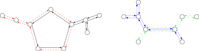
Figure 2. Four directed cycles giving two connected components: one double unicyclic (left) and one 2-4 tree (right).

Lemma 5.20 (Contributing graphs have multiple edges).

If $a_{\mathbf{k},t}(\pi)\neq 0$, edges of $G_{\pi,\mathbf{k}}$ are multiple.

Proof.

If one edge $(u,v)$ is single in $G_{\pi,\mathbf{k}}$, the random variable $a_{u,v}$ in centered and independent of the others so that $a_{\mathbf{k},t}(\pi)=0$. ∎

Lemma 5.21 (Graph characterisation of $q_{i,1},q_{i,2}$).

Suppose that $a_{\mathbf{k},t}(\pi)\neq 0$. For each connected component $\Gamma_{i}$:

• $q_{i,1}\leq 0$ with equality if and only if each edge in $\Gamma_{i}$ is double.

• $q_{i,2}\leq 1$ with equality if and only if $\overline{\Gamma_{i}}$ is a tree.

Proof.

Since each edge should be multiple by Lemma 5.20, to each edge in $\overline{\Gamma_{i}}$ corresponds at least two edges in $\Gamma_{i}$, so that $|E_{i}|\geq 2|\overline{E_{i}}|$. The equality case follows when every edge in $\overline{\Gamma_{i}}$ gives exactly two edges in $\Gamma_{i}$ which proves (a). The result (b) is a direct consequence of Proposition 5.4 (i). ∎

Lemma 5.22 (Even multiplicity of disconnecting edges).

Let $\overline{e}\in\overline{G_{\pi,\mathbf{k}}}$ corresponding to a set of twin edges in some connected component $\Gamma_{i}$. If the removal of the edges of $\overline{e}$ disconnects $\Gamma_{i}$, then the multiplicity of edges in $\overline{e}$ coming from each graph $G_{j}$ is an even number, with an equal number of edges in each direction.

Proof.

The proof uses the same arguments as in the proof of [23, Lemma 20]. Assume that a graph $G_{j}$ has $p\geq 1$ twin edges in the group $\overline{e}$ that disconnects $\Gamma_{i}$, for some $j\in[m]$ and $i\in I$.
Let us prove that $p>1$. Assume that $e_{0}\in G_{j}$ is the only one edge of $\overline{e}$ coming from $G_{j}$. The graph $G_{j}\setminus e_{0}$ is connected by construction of $G_{j}$. Then, in $\Gamma_{i}\setminus\overline{e}$ the source and target of $e_{0}$ are connected by the path in $G_{j}\setminus e_{0}$ which contradicts the assumption that $\overline{e}$ is disconnecting. Thus, $p>1$.
Assume $p\geq 2$. Start a walk in $G_{j}$ from the source of $e_{0}$ and consider $e_{1}$ its first twin edge in $G_{j}$ met after $e_{0}$. Then, $e_{0}$ and $e_{1}$ are opposite. Indeed, if they were parallel, removing $e_{0}$ and $e_{1}$ would not disconnect $G_{j}$. This would imply that removing $\overline{e}$ in $\overline{G_{\pi,\mathbf{k}}}$ would not disconnect $\Gamma_{i}$, leading to the same contradiction as in (i). Thus, $e_{0}$ and $e_{1}$ are opposite. Remove the loop from the source of $e_{0}$ to the target of $e_{1}$ in $G_{j}$. The remaining graph has now $p-2$ directed edges in $\overline{e}$. Using induction, one derives that the number of edges in $\overline{e}$ coming from $G_{j}$ is even with an equal number in each direction.

∎

Lemma 5.23 (Characterisation of non-vanishing connected components).

If $a_{\mathbf{k},t}(\pi)\neq 0$, then for every connected component $\Gamma_{i}$ of $G_{\pi,\mathbf{k}}$, one has $q_{i,1}+q_{i,2}\leq 0$ with equality if and only if the connected component is either double unicyclic of 2-4 tree type.

Before turning to the proof of Lemma 5.23, we will need the following lemmas.

Lemma 5.24 (Connectivity condition).

If there exists $j\in[m]$ and $i\in I$ such that $G_{j}=\Gamma_{i}$, then $a_{\mathbf{k},t}(\pi)=0$.

Proof.

For such $j\in[m]$ and $i\in I$ such that $G_{j}=\Gamma_{i}$, the random variable $(a_{\psi_{j}}-\mathbb{E}[a_{\psi_{j}}])$ is independent of the other random variables $\left\{(a_{\psi_{l}}-\mathbb{E}[a_{\psi_{l}}]):l\in[m],l\neq j\right\}$ and thus $a_{\mathbf{k},t}(\pi)=0$. ∎

Lemma 5.25 (Double tree type components have vanishing contribution).

If some connected component $\Gamma_{i}$ is of double tree type, then $a_{\mathbf{k},t}(\pi)=0$.

Proof.

Assume that $\Gamma_{i}$ is a connected component of double tree type. Let $E(\overline{\Gamma_{i}})$ be the edges of $\overline{\Gamma_{i}}$, each one corresponding to double opposite edges in $G_{\pi,\mathbf{k}}$. By Lemma 5.22, to each edge $\overline{e}\in E(\overline{\Gamma_{i}})$, one can associate some $j\in[m]$ such that the pair of opposite edges composing $\overline{e}$ comes from $G_{j}$ only. Denote this map $h:E(\overline{\Gamma_{i}})\rightarrow[m]$. If $h$ has more than one image point, say $j\neq l$ then $(a_{\psi_{j}}-\mathbb{E}[a_{\psi_{j}}])$ and $(a_{\psi_{l}}-\mathbb{E}[a_{\psi_{l}}])$ are independent of all other random variables and thus $a_{\mathbf{k},t}(\pi)=0$. If the image of $h$ contains only one integer $j\in[m]$, we would have $\Gamma_{i}=G_{j}$ so that $a_{\mathbf{k},t}(\pi)=0$ by Lemma 5.24. ∎

Proof of Lemma 5.23.

By the Lemmas 5.21 and 5.25 excluding double tree types, any connected component of a non-vanishing contribution satisfies $\Gamma_{i}$ satisfies $q_{i,1}+q_{i,2}<1$. The next possible value would be $q_{i,1}+q_{i,2}=\frac{1}{2}$ if $(q_{i,1},q_{i,2})=(-\frac{1}{2},1)$. Should the previous hold, the graph $\overline{\Gamma_{i}}$ would thus be a tree and $\Gamma_{i}$ would only have double edges except for an edge with multiplicity three, contradicting Lemma 5.22 as this group of edges would disconnect $G_{\pi,\mathbf{k}}$ and have an odd cardinal. Thus, we have $q_{i,1}+q_{i,2}\leq 0$, with equality cases corresponding to $\pi\in\mathcal{D}$ by the characterisations of Lemma 5.23. ∎

Proof of Proposition 5.19.

. The leading order of $n$ in $M^{(n)}_{\mathbf{k},t}$ is $q(\pi)=\sum_{i\in I}q_{i}(\pi)=\sum_{i\in I}q_{i,1}+q_{i,2}\leq 0$. By Lemma 5.23, the contribution of $\pi$ is non-vanishing if and only if each of its connected components are double unicyclic or 2-4 type which proves Proposition 5.19. ∎

5.4.3. Convergence to a Gaussian family

This section is devoted to the proof of Proposition 5.15. To prove that the limiting family is Gaussian, let us write $M^{(n)}_{\mathbf{k},t}$ as a Wick product. This is the statement of Proposition 5.27 below which is the analogue of [23, Proposition 33]. Such an expression implies that the family is Gaussian and thus proves Proposition 5.15. Our proof structure follows again the lines of [23].

Definition 5.26.

For any pair of indexes $\{j,l\}$, denote $\mathcal{P}(j,l)$ the set of partitions $\pi$ of $\{k_{j-1}+1,\dots,k_{j}]\}\cup\{k_{l-1}+1,\dots,k_{l}\}$ such that

• Either the graph $G_{j}\cup G_{l}$ is of double unicyclic type and both graphs $\overline{G_{j}}$, $\overline{G_{l}}$ are unicyclic. This happens when both graphs $G_{j}$ and $G_{l}$ are double unicyclic trees with the same cycle, by pairing the edges in the common cycle.

• Either $G_{j}\cup G_{l}$ is of 2-4 tree type and both graphs $G_{j}$, $G_{l}$ are double trees. A pair of twin edges in $G_{j}$ and a pair of twin edges $G_{l}$ are thus paired to form the group of edges of multiplicity four in $G_{j}\cup G_{l}$.

The following proposition shows that graphs contributing to the limit in $M^{(n)}_{\mathbf{k},t}$ are obtained by pairing the graphs $\{G_{j}\}_{1\leq j\leq m}$.

Proposition 5.27 (Wick product expression of $M^{(n)}_{\mathbf{k},t}$).

We have

(5.19) $$M^{(n)}_{\mathbf{k},t}=\sum_{\sigma\in\mathcal{P}_{2}(m)}\prod_{(j,l)\in\sigma}M_{t}(j,l)+o(1)$$

as $n\rightarrow+\infty$, with

(5.20) $$M_{t}(j,l)=\sum_{\pi\in\mathcal{P}(j,l)}a_{t}(\pi)$$

where $a_{t}(\pi)$ is the common value for $\mathbb{E}\left[(a_{\psi_{j}}-\mathbb{E}[a_{\psi_{j}}])^{(s_{j})}(a_{\psi_{l}}-\mathbb{E}[a_{\psi_{l}}])^{(s_{l})}\right]$ for $\psi_{j},\psi_{k}$ such that the associated partition of $\{k_{j-1}+1,\dots,k_{j}\}\cup\{k_{l-1}+1,\dots,k_{l}\}$ is $\pi$.

The proof of Proposition 5.27 relies on Lemma 5.28 that we state below. Recall that by Proposition 5.19, the only graphs $G_{1},\dots,G_{m}$ that can contribute are those for which their union graph has connected components of either double unicyclic or 2-4 type. As products are centered, each such connected component should come from at least two of the $G_{i}$’s. The next lemma adapted from [23, Lemma 35] shows that each connected component comes from exactly two of the $G_{i}$’s, which is where the pairings appear.

Lemma 5.28 (Graph pairings).

Consider $\pi\in\mathcal{P}(k)$ such that $a_{\mathbf{k},t}(\pi)\neq 0$ and assume that $\Gamma_{i}$ is of double cycle type. Then, there are two different cycles $G_{j}$, $G_{l}$ such that each group of twin edges in the cycle of $\Gamma_{i}$ consists in an edge from $G_{j}$ and an edge from $G_{l}$.

Proof.

Denote $E_{0}$ the set of groups of twin edges in the cycle of $\Gamma_{i}$. Assume that some $G_{j}$ has exactly one edge in a group $\overline{e}\in E_{0}$. Suppose for the sake of a contradiction that there is another group of edge $\overline{e}^{\prime}\in E_{0}$ coming from two other cycles $G_{j^{\prime}},G_{j^{\prime\prime}}$ with $j^{\prime}\neq j\neq j^{\prime\prime}$. The removal of $\overline{e}$ disconnects $G_{\pi,\mathbf{k}}\setminus\overline{e}^{\prime}$ (which is connected). The fact that only one edge of $\overline{e}$ comes from $G_{j}$ would contradict 5.22. Thus, $G_{j}$ has one edge in every element of $E_{0}$ and since $\Gamma_{i}$ is a double cycle, there is some other cycle $G_{l}$ with the same property. Let us show that this other cycle cannot be $G_{j}$.
Assume now that each group in $E_{0}$ comes from only a single cycle $G_{j}$. Then, the component $\Gamma_{i}$ would come from this cycle $G_{j}$ and thus $G_{j}$ would be X disconnected from $G_{\pi,\mathbf{k}}$ giving $a_{\mathbf{k},t}(\pi)=0$. ∎

Proof of Proposition 5.27.

. Assume that some component $\Gamma_{i}$ of $G_{\pi,\mathbf{k}}$ is made from at least three cycles among $G_{1},\dots,G_{m}$. We will show that $a_{\mathbf{k},t}(\pi)=0$.

• If $\Gamma_{i}$ is a 2-4 type, by Lemma 5.22, the edge of multiplicity four can only come from two graphs $G_{j},G_{l}$ and one of the (at least) three graphs would be disconnected leading to a vanishing contribution.

• If $\Gamma_{i}$ is double unicyclic, Lemma 5.28 shows that there are two graphs that are paired to constitute its cycle. Since every other edge has multiplicity two outside the cycle, one would also have at least one disconnected graph and a vanishing contribution.

Thus, the only non-vanishing contributions come from a pairing of unicyclic double trees $G_{j},G_{l}$ paired together to form either a double unicyclic graph and a 2-4 tree. ∎

By Iserlis-Wick’s lemma, the proof of Proposition 5.15 is complete.

5.4.4. Computation of the limiting covariance

To prove Proposition 5.16, we need to compute the asymptotic covariance of the previous Gaussian family and show that it is diagonal for the modified Chebyshev polynomials. Let us take $m=2$ and consider $\pi\in\mathcal{P}(1,2)$ a partition associated to any function $\psi$ such that the associated union graph $G_{\pi,\mathbf{k}}=G_{k_{1}}\cup G_{k_{2}}$ is a double unycylic graph or a 2-4 tree. Let us compute the value of

$$a_{t}(\pi)=\mathbb{E}\left[(a_{\psi_{1}}-\mathbb{E}[a_{\psi_{1}}])^{(s_{1})}(a_{\psi_{2}}-\mathbb{E}[a_{\psi_{2}}])^{(s_{2})}\right].$$

If $G_{\pi,\mathbf{k}}$ is of double unicycle type, then $G_{k_{1}}$ and $G_{k_{2}}$ are unicyclic double trees with the same cycle, either in the same direction or opposite. If they are opposite (respectively parallel), we say that $\pi\in DU^{opp}$ (respectively $\pi\in DU^{par}$).

Lemma 5.29 (Covariance $\varphi^{(t)}(X^{k_{1}},X^{k_{2}})$).

Let us fix $s_{1}=s_{2}=0$ and suppose that $G_{\pi,\mathbf{k}}$ is a double unicyclic graph with a cycle of length $l\geq 1$.

• If $\pi\in DU^{opp},a_{t}(\pi)=t^{(k_{1}+k_{2})/2}$.

• If $\pi\in DU^{par},a_{t}(\pi)=t^{(k_{1}+k_{2})/2}\delta_{l=1}$.

• If $\pi\in FT,a_{t}(\pi)=t^{(k_{1}+k_{2})/2}$.

Proof.

Suppose that $G_{\pi,\mathbf{k}}\in DU^{opp}$. Then, the cycle length $l$ is at least $3$ since a cycle of length $2$ would only belong to one of the graphs $G_{k_{1}},G_{k_{2}}$ and the two graphs would be independent of each other. Each of $G_{k_{1}}$ and $G_{k_{2}}$ both have $l$ simple edges so that $\mathbb{E}[a_{\psi_{1}}]=\mathbb{E}[a_{\psi_{2}}]=0$. Moreover, $a_{\psi_{1}}a_{\psi_{2}}$ is the product of $\frac{k_{1}+k_{2}}{2}$ independent variables with the same distribution as $a_{1,2}a_{2,1}$ which gives $(i)$. For $G_{\pi,\mathbf{k}}\in DU^{par}$, if $l\neq 1$, since $\mathbb{E}[a_{1,2}^{2}]=0$, one would have $a_{t}(\pi)=0$. The only parallel contribution comes from $l=1$ where the cycle of $G_{\pi,\mathbf{k}}$ is a double loop edge which gives $\mathbb{E}[a_{1,1}^{2}]=t$ and thus $a_{t}(\pi)=t\cdot t^{(k_{1}+k_{2})/2-1}=t^{(k_{1}+k_{2})/2}$ proving $(ii)$. If $G_{\pi,\mathbf{k}}\in FT$, the quadruple edge gives a contribution of $\mathbb{E}[a_{1,2}^{2}a_{2,1}^{2}]=2t^{2}$ while other opposite edges give a contribution of $t$. Therefore, $\mathbb{E}[a_{\psi_{1}}a_{\psi_{2}}-\mathbb{E}[a_{\psi_{1}}a_{\psi_{2}}]]=(2t^{2}-t^{2})t^{(k_{1}+k_{2})/2-2}$ which proves $(iii)$. ∎

Lemma 5.30 (Covariance $\varphi^{(t)}_{c}(X^{k_{1}},X^{k_{2}})$).

Let us fix $s_{1}=0$ and $s_{2}=1$. We have, where $l$ is the common cycle length.

• If $\pi\in DU^{opp},a_{t}(\pi)=0$.

• If $\pi\in DU^{par},a_{t}(\pi)=t^{(k_{1}+k_{2})/2-l}$.

• If $\pi\in FT,a_{t}(\pi)=t^{(k_{1}+k_{2})/2-2}$.

Proof.

We have $\mathbb{E}[a_{1,2}\overline{a_{2,1}}]=0$ so any opposite cycle has zero expectation proving $(i)$. For $G_{\pi,\mathbf{k}}\in DU^{par}$, since $\mathbb{E}[a_{1,2}\overline{a_{1,2}}]=\mathbb{E}|a_{1,2}|^{2}=1=\mathbb{E}|a_{1,1}|^{2}$ and the rest of the double edges outside the cycle have expectation $t$, one derives $(ii)$. If $G_{\pi,\mathbf{k}}\in FT$, the quadruple edge gives a contribution of $\mathbb{E}[|a_{1,2}|^{2}|a_{2,1}|^{2}]=1+t^{2}$ so that $a_{t}(\pi)=t^{(k_{1}+k_{2})/2-2}(\mathbb{E}[|a_{1,2}|^{2}|a_{2,1}|^{2}]-t^{2})=t^{(k_{1}+k_{2})/2-2}$. ∎

We are now interested in the number of partitions in $\mathcal{P}(i,j)$. In [23, Lemma 39], the authors introduced a bijection that allows us to count the number of double unicyclic graphs as well as the number of 2-4 trees. Let us first assume that $k_{1}$ and $k_{2}$ are both even. Recall that they necessarily have the same parity. Define $\mathcal{G}_{2l}$ the set of all possible graphs obtained which are of double unicyclic type having a cycle length of $2l$ for $l\geq 1$. We state the result of [23, Lemma 39], as well as its extension to $2-4$ tree types as discussed after [23, Definition 40].

Lemma 5.31 (Non-crossing annular pairings enumeration).

For each $l\geq 1$, there is a bijection from $\mathcal{G}_{2l}$ to the set $NC_{2}^{(l)}(k_{1},k_{2})$ of non crossing pairings of the $k_{1},k_{2}$ annulus with $l$ through strings.
Furthermore, there is a bijection from $\mathcal{FT}$ to the set $NC_{2}^{(2)}(k_{1},k_{2})$ of non crossing pairings of the $k_{1},k_{2}$ annulus with $2$ through strings.

Denote $nc^{(l)}(p,q)$ the cardinal of $NC_{2}^{(l)}(p,q)$. By [24, Proof of Lemma 22] and reference [26] therein one can have an explicit expression of this quantity given by

(5.21) $$nc^{(l)}(p,q)=l\binom{p}{\frac{p-l}{2}}\binom{q}{\frac{q-l}{2}}.$$

We summarise the results of this section for the value of $M_{t}(k_{1},k_{2})$ in the table below.

	$s_{0}=s_{1}=0$	$s_{0}=0,s_{1}=1$
$k_{1},k_{2}$ even	$\sum_{l=1}^{k_{1}/2}nc^{(2l)}(k_{1},k_{2})t^{(k_{1}+k_{2})/2}$	$\sum_{l=1}^{k_{1}/2}nc^{(2l)}(k_{1},k_{2})t^{(k_{1}+k_{2})/2-2l}$
$k_{1},k_{2}$ odd	$\sum_{l=1}^{(k_{1}+1)/2}nc^{(2l-1)}(k_{1},k_{2})t^{(k_{1}+k_{2})/2}$	$\sum_{l=1}^{(k_{1}+1)/2}nc^{(2l-1)}(k_{1},k_{2})t^{(k_{1}+k_{2})/2-2l+1}$

Table 1. Values of $M_{t}(k_{1},k_{2})$.

To end the proof of Proposition 5.16, we need to compute $\varphi^{(t)}(P^{(t)}_{k},P^{(t)}_{l})$ and $\varphi^{(t)}_{c}(P^{(t)}_{k},P^{(t)}_{l})$ to show that those quantities vanish when $k\neq l$. For any $t\in[0,1]$ and $k\geq 0$, we have

$$P^{(t)}_{k}=\sum_{j=0}^{k/2}\alpha^{(k,t)}_{k-2j}X^{k-2j},$$

where the coefficients $\left(\alpha^{(k,t)}_{k-2j}\right)_{k,j}$ are those of (5.9). Recall the followings facts:

• $\varphi^{(1)}$ is diagonalized by the usual Chebyshev polynomials $\{P^{(1)}_{k}\}_{k\geq 1}$, see [25, Theorem 5.1], so that one has:

  (5.22) $$\varphi^{(1)}(P^{(1)}_{k},P^{(1)}_{l})=k\delta_{k=l}.$$

• We have the scaling relation: $P^{(t)}_{k}(x)=\sqrt{t}^{k}P^{(1)}_{k}\left(\frac{x}{\sqrt{t}}\right)$, so that $\alpha^{(k,t)}_{k-2j}=\sqrt{t}^{2j}\alpha^{(k,1)}_{k-2j}$.

Since $\varphi^{(t)}(X^{p},X^{q})=\sqrt{t}^{p+q}\varphi^{(1)}(X^{p},X^{q})=nc(p,q)\sqrt{t}^{p+q}$, for every $k,l\geq 1$ one has,

$$\varphi^{(t)}(P^{(t)}_{k},P^{(t)}_{l}) =\sum_{i,j}\alpha^{(k,t)}_{k-2i}\alpha^{(l,t)}_{l-2j}\varphi^{(t)}(X^{k-2i},X^{l-2j})$$

$$=\sum_{i,j}\alpha^{(k,t)}_{k-2i}\alpha^{(l,t)}_{l-2j}\sqrt{t}^{k+l-2i-2j}\varphi^{(1)}(X^{k-2i},X^{l-2j})$$

$$=\sum_{i,j}\alpha^{(k,1)}_{k-2i}\alpha^{(l,1)}_{l-2j}\sqrt{t}^{k+l}\varphi^{(1)}(X^{k-2i},X^{l-2j})$$

$$=\sqrt{t}^{k+l}\varphi^{(1)}(P^{(1)}_{k},P^{(1)}_{l})$$

$$=k\sqrt{t}^{k+l}\delta_{k=l}$$

which proves (5.15). It remains to prove (5.16). Suppose that $k_{1}\leftarrow 2k_{1}$ and $k_{2}\leftarrow 2k_{2}$ are both even. Then,

$$\varphi_{c}^{(t)}(P_{2k_{1}}^{(t)},P_{2k_{2}}^{(t)}) =\sum_{r,s\geq 0}\alpha^{(2k_{1},t)}_{2k_{1}-2r}\alpha^{(2k_{2},t)}_{2k_{2}-2s}\varphi_{c}^{(t)}(X^{2k_{1}-2r},X^{2k_{2}-2s})$$

$$=\sum_{r,s\geq 0}\alpha^{(2k_{1},t)}_{2k_{1}-2r}\alpha^{(2k_{2},t)}_{2k_{2}-2s}\sum_{l\geq 1}nc^{(2l)}(2k_{1}-2r,2k_{2}-2s)t^{\frac{2k_{1}+2k_{2}}{2}-(r+s+2l)}$$

$$=\sum_{l\geq 1}t^{k_{1}+k_{2}-2l}\sum_{r,s\geq 0}\alpha^{(2k_{1},1)}_{2k_{1}-2r}\alpha^{(2k_{2},1)}_{2k_{2}-2s}nc^{(2l)}(2k_{1}-2r,2k_{2}-2s).$$

Let $l\geq 1$ be fixed. For $r\leq k_{1}-l$, $s\leq k_{2}-l$ using (5.21), the innermost sum is

$$\sum_{r,s\geq 0}\alpha^{(2k_{1},1)}_{2k_{1}-2r}\alpha^{(2k_{2},1)}_{2k_{2}-2s}nc^{(2l)}(2k_{1}-2r,2k_{2}-2s)$$

$$=(2k_{1}\cdot 2k_{2}\cdot 2l)\sum_{r,s\geq 0}\frac{(-1)^{r+s}}{(2k_{1}-r)(2k_{2}-s)}\binom{2(k_{1}-r)}{k_{1}-r-l}\binom{2(k_{2}-s)}{k_{2}-s-l}\binom{2k_{1}-r}{r}\binom{2k_{2}-s}{s}$$

(5.23) $$=8lk_{1}k_{2}\left(\sum_{r=0}^{k_{1}-l}\frac{(-1)^{r}}{(2k_{1}-r)}\binom{2(k_{1}-r)}{k_{1}-r-l}\binom{2k_{1}-r}{r}\right)\left(\sum_{s=0}^{k_{2}-l}\frac{(-1)^{s}}{(2k_{2}-s)}\binom{2(k_{2}-s)}{k_{2}-s-l}\binom{2k_{2}-s}{s}\right).$$

We claim that if $k_{1}\neq k_{2}$, one of the two sums in (5.23) is zero. Let us take $k\geq l+1$. One has

(5.24) $$\sum_{r=0}^{k-l}\frac{(-1)^{r}}{(2k-r)}\binom{2(k-r)}{k-r-l}\binom{2k-r}{r} =\sum_{r=0}^{k-l}\frac{(-1)^{r}}{(2k-r)}\binom{k-l}{r}\binom{2k-r}{k-l}$$

(5.25) $$=\frac{1}{k-l}\sum_{r=0}^{k-l}(-1)^{r}\binom{k-l}{r}\binom{2k-r-1}{k+l-r}.$$

The binomial coefficient $\binom{2k-r-1}{k+l-r}$ is the coefficient of $z^{k+l-r}$ in the development of $(1+z)^{2k-r-1}$. Thus, the sum (5.25) is the coefficient of $z^{k+l}$ in the development of $Q(z)=\sum_{r=0}^{k-l}(-1)^{r}\binom{k-l}{r}(1+z)^{2k-r-1}z^{r}$. However,

$$Q(z)=(1+z)^{2k-1}\sum_{r=0}^{k-l}\binom{k-l}{r}\left(\frac{-z}{1+z}\right)^{r}=(1+z)^{k+l-1}$$

so that the coefficient of $z^{k+l}$ in $Q(z)$ is zero. If $k_{1}=k_{2}=l$, the two sums in (5.23) are equal to $\frac{1}{2l}$ so that

(5.26) $$\varphi_{c}^{(t)}(P_{2k_{1}}^{(t)},P_{2k_{2}}^{(t)})=(2k_{1})\delta_{k_{1}=k_{2}}$$

which is (5.16) for even indexes. The computations are essentially the same for odd values of $k_{1}\leftarrow 2k_{1}+1$ and $k_{2}\leftarrow 2k_{2}+1$:

(5.27) $$\varphi_{c}^{(t)}(P_{2k_{1}+1}^{(t)},P_{2k_{2}+1}^{(t)}) =\sum_{r,s\geq 0}\alpha^{(2k_{1}+1,t)}_{2k_{1}+1-2r}\alpha^{(2k_{2}+1,t)}_{2k_{2}+1-2s}\varphi_{c}^{(t)}(X^{2k_{1}+1-2r},X^{2k_{2}+1-2s})$$

(5.28) $$=\sum_{l\geq 1}t^{k_{1}+k_{2}-2l+2}\sum_{r,s\geq 0}\alpha^{(2k_{1}+1,1)}_{2k_{1}+1-2r}\alpha^{(2k_{2}+1,1)}_{2k_{2}+1-2s}nc^{(2l-1)}(2k_{1}+1-2r,2k_{2}+1-2s).$$

For a fixed value of $l\geq 1$, the innermost sum is

$$\sum_{r,s\geq 0}\alpha^{(2k_{1}+1,1)}_{2k_{1}+1-2r}\alpha^{(2k_{2}+1,1)}_{2k_{2}+1-2s}nc^{(2l-1)}(2k_{1}+1-2r,2k_{2}+1-2s)=(2k_{1}+1)(2k_{2}+1)(2l-1)\times$$

$$\sum_{r,s\geq 0}\frac{(-1)^{r+s}}{(2k_{1}+1-r)(2k_{2}+1-s)}\binom{2(k_{1}-r)+1}{k_{1}+1-r-l}\binom{2(k_{2}-s)+1}{k_{2}+1-s-l}\binom{2k_{1}+1-r}{r}\binom{2k_{2}+1-s}{s}$$

(5.29) $$=\left(\sum_{r=0}^{k_{1}+1-l}\frac{(-1)^{r}}{(2k_{1}+1-r)}\binom{2(k_{1}-r)+1}{k_{1}+1-r-l}\binom{2k_{1}+1-r}{r}\right)\left(\sum_{s=0}^{k_{2}+1-l}\frac{(-1)^{s}}{(2k_{2}-s)}\binom{2(k_{2}-s)+1}{k_{2}+1-s-l}\binom{2k_{2}+1-s}{s}\right)$$

$$\times(2k_{1}+1)(2k_{2}+1)(2l-1).$$

Using the same argument as above, the two sums in (5.29) vanish, except when $k_{1}+1=k_{2}+1=l$ where they are both equal to $\frac{1}{2l+1}$. Therefore,

(5.30) $$\varphi_{c}^{(t)}(P_{2k_{1}+1}^{(t)},P_{2k_{2}+1}^{(t)})=(2k_{1}+1)\delta_{k_{1}=k_{2}},$$

which ends the proof of statement (5.16) in Proposition 5.16.

Remark 5.32.

Let us verify that for $t=0$, one finds the result of [12]. We have that

$$\varphi^{(t)}(P^{(t)}_{k},P^{(t)}_{l})=0$$

according to Proposition 5.16 which is indeed equal to $\mathbb{E}[a_{1,2}^{2}]^{k}=0$. On the other hand,

$$\varphi^{(t)}_{c}(X^{p},X^{q})=nc^{(p)}(p,q)\delta_{p,q}=p\delta_{p,q}$$

where the last equality comes from the fact that a non-crossing pairing of the $(p,p)$ annulus with $p$ through strings is determined by the choice of one through string only. Thus, $(V^{(n)}_{k})_{k}$ converges to a Gaussian family $(V_{k})_{k}$ of independent centered variables with parameters $\mathbb{E}[|V_{k}|^{2}]=k$, $\mathbb{E}[V_{k}^{2}]=0$ which coincides with the Gaussian family in [12, Theorem 1.2].

References

• [1] G. Akemann, M. Duits and L.. Molag “The elliptic Ginibre ensemble: a unifying approach to local and global statistics for higher dimensions” In J. Math. Phys. 64.2, 2023, pp. 023503\bibrangessep39 DOI: 10.1063/5.0089789
• [2] G. Akemann and G. Vernizzi “Characteristic polynomials of complex random matrix models” In Nuclear Physics B 660.3 Elsevier BV, 2003, pp. 532–556 DOI: 10.1016/s0550-3213(03)00221-9
• [3] Yacin Ameur and Joakim Cronvall “Szegő type asymptotics for the reproducing kernel in spaces of full-plane weighted polynomials” In Comm. Math. Phys. 398.3, 2023, pp. 1291–1348 DOI: 10.1007/s00220-022-04539-y
• [4] Yacin Ameur, Haakan Hedenmalm and Nikolai Makarov “Random normal matrices and Ward identities” In Ann. Probab. 43.3, 2015, pp. 1157–1201 DOI: 10.1214/13-AOP885
• [5] G.. Anderson and O. Zeitouni “A CLT for a band matrix model” In Probab. Theory Relat. Fields 134.2, 2006, pp. 283–338 DOI: 10.1007/s00440-004-0422-3
• [6] Z. Bai and J.. Silverstein “Spectral analysis of large dimensional random matrices”, Springer Ser. Stat. Dordrecht: Springer, 2010 DOI: 10.1007/978-1-4419-0661-8
• [7] Z.. Bai and J.. Silverstein “CLT for linear spectral statistics of large-dimensional sample covariance matrices.” In Ann. Probab. 32.1A, 2004, pp. 553–605 DOI: 10.1214/aop/1078415845
• [8] Z.. Bai and J. Yao “On the convergence of the spectral empirical process of Wigner matrices” In Bernoulli 11.6, 2005, pp. 1059–1092 DOI: 10.3150/bj/1137421640
• [9] A. Basak and O. Zeitouni “Outliers of random perturbations of Toeplitz matrices with finite symbols” In Probab. Theory Relat. Fields 178.3-4, 2020, pp. 771–826 DOI: 10.1007/s00440-020-00990-x
• [10] M. Bender “Edge scaling limits for a family of non-Hermitian random matrix ensembles” In Probab. Theory Relat. Fields 147.1-2, 2010, pp. 241–271 DOI: 10.1007/s00440-009-0207-9
• [11] C. Bordenave and D. Chafai “Around the circular law” In Probab. Surv. 9, 2012, pp. 1–89 DOI: 10.1214/11-PS183
• [12] C. Bordenave, D. Chafai and D. García-Zelada “Convergence of the spectral radius of a random matrix through its characteristic polynomial” In Probab. Theory Relat. Fields 182.3-4, 2022, pp. 1163–1181 DOI: 10.1007/s00440-021-01079-9
• [13] R. Chhaibi, J. Najnudel and A. Nikeghbali “The circular unitary ensemble and the Riemann zeta function: the microscopic landscape and a new approach to ratios” In Inventiones mathematicae 207.1 Springer ScienceBusiness Media LLC, 2016, pp. 23–113 DOI: 10.1007/s00222-016-0669-1
• [14] S. Coste “Sparse matrices: convergence of the characteristic polynomial seen from infinity” Id/No 8 In Electron. J. Probab. 28, 2023, pp. 40 DOI: 10.1214/22-EJP875
• [15] Persi Diaconis and Mehrdad Shahshahani “On the eigenvalues of random matrices” Studies in applied probability In J. Appl. Probab. 31A, 1994, pp. 49–62 DOI: 10.2307/3214948
• [16] V.. Girko “Elliptic law” In Theory Probab. Appl. 30, 1986, pp. 677–690 DOI: 10.1137/1130089
• [17] V.. Girko “The elliptic law: Ten years later. I” In Random Oper. Stoch. Equ. 3.3, 1995, pp. 257–302 DOI: 10.1515/rose.1995.3.3.257
• [18] S. Janson and K. Nowicki “The asymptotic distributions of generalized U-statistics with applications to random graphs” In Probab. Theory Relat. Fields 90.3, 1991, pp. 341–375 DOI: 10.1007/BF01193750
• [19] K. Johansson “From Gumbel to Tracy-Widom” In Probab. Theory Relat. Fields 138.1-2, 2007, pp. 75–112 DOI: 10.1007/s00440-006-0012-7
• [20] K. Johansson “On fluctuations of eigenvalues of random Hermitian matrices.” In Duke Math. J. 91.1, 1998, pp. 151–204 DOI: 10.1215/S0012-7094-98-09108-6
• [21] D. Jonsson “Some limit theorems for the eigenvalues of a sample covariance matrix” In J. Multivariate Anal. 12, 1982, pp. 1–38 DOI: 10.1016/0047-259X(82)90080-X
• [22] Boris Khoruzhenko and Hans-Jurgen Sommers “Non-Hermitian ensembles” In The Oxford Handbook of Random Matrix Theory Oxford University Press, 2015 DOI: 10.1093/oxfordhb/9780198744191.013.18
• [23] C. Male, J.. Mingo, S. Péché and R. Speicher “Joint global fluctuations of complex Wigner and deterministic matrices” Id/No 2250015 In Random Matrices Theory Appl. 11.2, 2022, pp. 46 DOI: 10.1142/S2010326322500150
• [24] J.. Mingo “Non-crossing annular pairings and the infinitesimal distribution of the GOE” In J. Lond. Math. Soc., II. Ser. 100.3, 2019, pp. 987–1012 DOI: 10.1112/jlms.12253
• [25] J.. Mingo and R. Speicher “Free probability and random matrices” 35, Fields Inst. Monogr. Toronto: The Fields Institute for Research in the Mathematical Sciences; New York, NY: Springer, 2017 DOI: 10.1007/978-1-4939-6942-5
• [26] J.. Mingo, R. Speicher and E. Tan “Second order cumulants of products” In Trans. Am. Math. Soc. 361.9, 2009, pp. 4751–4781 DOI: 10.1090/S0002-9947-09-04696-0
• [27] A.. Naumov “The elliptic law for random matrices” In Vestnik Moskov. Univ. Ser. XV Vychisl. Mat. Kibernet., 2013, pp. 31–38\bibrangessep48
• [28] H.. Nguyen and S. O’Rourke “The elliptic law” In Int. Math. Res. Not. 2015.17, 2015, pp. 7620–7689 DOI: 10.1093/imrn/rnu174
• [29] M. Noy “Graph enumeration” In Handbook of enumerative combinatorics Boca Raton, FL: CRC Press, 2015, pp. 397–436
• [30] S. O’Rourke and D. Renfrew “Low rank perturbations of large elliptic random matrices” Id/No 43 In Electron. J. Probab. 19, 2014, pp. 65 DOI: 10.1214/EJP.v19-3057
• [31] B. Rider “A limit theorem at the edge of a non-Hermitian random matrix ensemble” In J. Phys. A, Math. Gen. 36.12, 2003, pp. 3401–3409 DOI: 10.1088/0305-4470/36/12/331
• [32] T. Shirai “Limit theorems for random analytic functions and their zeros” In RIMS Kôkyûroku Bessatsu B34, 2012, pp. 335–359
• [33] Y. Sinai and A. Soshnikov “Central limit theorem for traces of large random symmetric matrices with independent matrix elements” In Bol. Soc. Bras. Mat., Nova Sér. 29.1, 1998, pp. 1–24 DOI: 10.1007/BF01245866
• [34] H.. Sommers, A. Crisanti, H. Sompolinsky and Y. Stein “Spectrum of Large Random Asymmetric Matrices” In Phys. Rev. Lett. 60 American Physical Society, 1988, pp. 1895–1898 DOI: 10.1103/PhysRevLett.60.1895
• [35] G. Szegö “Orthogonal polynomials. 4th ed” 23, Colloq. Publ., Am. Math. Soc. Providence, RI: American Mathematical Society (AMS), 1975
• [36] Craig Tracy and Harold Widom “Distribution functions for largest eigenvalues and their applications” In Proceedings of the ICM 1, 2002