Understanding Pathologies of Deep Heteroskedastic Regression
Abstract
Deep, overparameterized regression models are notorious for their tendency to overfit. This problem is exacerbated in heteroskedastic models, which predict both mean and residual noise for each data point. At one extreme, these models fit all training data perfectly, eliminating residual noise entirely; at the other, they overfit the residual noise while predicting a constant, uninformative mean. We observe a lack of middle ground, suggesting a phase transition dependent on model regularization strength. Empirical verification supports this conjecture by fitting numerous models with varying mean and variance regularization. To explain the transition, we develop a theoretical framework based on a statistical field theory, yielding qualitative agreement with experiments. As a practical consequence, our analysis simplifies hyperparameter tuning from a two-dimensional to a one-dimensional search, substantially reducing the computational burden. Experiments on diverse datasets, including UCI datasets and the large-scale ClimSim climate dataset, demonstrate significantly improved performance in various calibration tasks.
1 Introduction
Homoskedastic regression models assume constant (e.g., Gaussian) output noise and amount to learning a function that tries to predict the most likely target for input . In contrast, heteroskedastic models assume that the output noise may depend on the input features as well, and try to learn a conditional distribution with non-uniform variance. The promise of this approach is to assign different importances to training data and to train models that “know where they fail” [Skafte et al., 2019, Fortuin et al., 2022].
Unfortunately, overparameterized heteroskedastic regression models (e.g., based on deep neural networks) are prone to extreme forms of overfitting [Lakshminarayanan et al., 2017, Nix and Weigend, 1994]. On the one hand, the mean model is flexible enough to fit every training datum’s target perfectly, while the standard deviation network learns to maximize the likelihood by shrinking the predicted standard deviations to zero. On the other hand, just the tiniest amount of regularization on the mean network will make the model prefer a constant solution. Such a flat prediction results from the standard deviation network’s ability to explain all residuals as random noise, thus overfitting the data’s empirical prediction residuals. Fig. 1 shows both types of overfitting.
While several practical solutions to learning overparameterized heteroskedastic regression models have been proposed [Skafte et al., 2019, Stirn and Knowles, 2020, Seitzer et al., 2022, Stirn et al., 2023, Immer et al., 2023], no comprehensive theoretical study of the failure of these methods has been offered so far. We conjecture this is because overparameterized models have attracted the most attention only in the past few years, while most classical statistics have focused on under-parameterized (e.g., linear) regression models where such problems cannot occur [Huber, 1967, Astivia and Zumbo, 2019].
This paper provides a theoretical analysis of the failure of heteroskedastic regression models in the overparameterized limit. To this end, it borrows a tool that abstracts away from any details of the involved neural network architectures: classical field theory from statistical mechanics [Landau and Lifshitz, 2013, Altland and Simons, 2010]. Via our field-theoretical description, we can recover the optimized heteroskedastic regressors as solutions to partial differential equations that can be derived from a variational principle. These equations can in turn be solved numerically by optimizing the field theory’s free energy functional.
Our analysis results in a two-dimensional phase diagram, representing the coarse-grained behavior of heteroskedastic noise models for every parameter configuration. Each of the two dimensions corresponds to a different level of regularization of either the mean or standard deviation network. As encountered in many complex physical systems, the field theory unveils phase transitions, i.e., sudden and discontinuous changes in certain observables (metrics of interest) that characterize the model, such as the smoothness of its mean prediction network, upon small changes in the regularization strengths. In particular, we find a sharp phase boundary between the two types of behavior outlined in the first paragraph, at weak regularization.
Our contributions are as follows:
-
•
We provide a unified theoretical description of overparameterized heteroskedastic regression models, which generalizes across different models and architectures, drawing on tools from statistical mechanics and variational calculus.
-
•
In this framework, we derive a field theory (FT), which can explain the observed types of overfitting in these models and describe phase transitions between them. We show qualitative agreement of our FT with experiments, both on simulated and real-world regression tasks.
-
•
As a practical consequence of our analysis, we dramatically reduce the search space over hyperparameters by eliminating one parameter. This reduces the number of hyperparameters from two to one, empirically resulting in well-calibrated models. We demonstrate the benefits of our approach on a large-scale climate modeling example.
2 Pitfalls of Overparameterized Heteroskedastic Regression
Heteroskedastic Regression
Consider the setting in which we have a collection of independent data points with covariates drawn from some distribution and response values normally distributed with unique mean and precision (inverse-variance) (i.e., ). We assume to be in a heteroskedastic setting, in which need not equal for . Finally, we assume both the mean and standard deviation of to be explainable via :
| (1) |
with continuous functions and . In a modeling setting, learning can be seen as directly estimating and quantifying the aleatoric (data) uncertainty.
Overparameterized Neural Networks
There exist many options for modeling and . Of particular interest to many is representing each of these functions as neural networks [Nix and Weigend, 1994]—specifically ones that are overparameterized. These models are well-known universal function approximators, which makes them great choices for estimating the true functions and [Hornik, 1991].
Let the mean network and precision network be arbitrary depth, overparameterized feed-forward neural networks parameterized by and respectively. For a given input , these networks collectively represent a corresponding predictive distribution for :
| (2) |

Pitfalls of MLE
Our assumed form of data naturally suggests training and , or rather learning and , by minimizing the cross-entropy between the joint data distribution and the induced predictive distribution . This objective is defined as
| (3) | ||||
where is a constant with respect to and . This expectation is often approximated using a Monte Carlo (MC) estimate with samples, yielding the following tractable objective function:
| (4) |
where . Minimizing this cross-entropy objective function with respect to parameters and using data samples is synonymous with maximum likelihood estimation (MLE).
Unfortunately, given an infinitely flexible model, this objective function is ill-posed. Our first observation is that, for any non-zero , we can find a solution for the parameters in the absence of any regularization since the first term in Eq. 4 is minimized when , while the second term is minimized when . However, the interplay between and leads to divergences in the absence of any regularization on . Without such regularization, the mean function will estimate perfectly (or rather to arbitrary precision) for at least a single data point . Once this happens, the residual for this input approaches zero, and the implicit regularization for vanishes, leading to diverge to infinity. Intuitively, the model becomes infinitely (over-)confident in its prediction for this data point. Once training has reached this point, the objective function becomes completely unstable due to effectively containing a term whose limit naïvely yields .111Note that this is predicated on the model being flexible enough to allow for large changes in predictions and after iteratively updating parameters and while allowing for minimal changes in neighboring predictions (i.e., and for some such that ).
Regularization
Even though is implicitly regularized in the standard cross-entropy loss as mentioned earlier, we posit that additional regularization on , or rather , is required to avoid this instability. It can be tempting to think that one must regularize in order to avoid overfitting. And while this is generally true, the objective function will still be unstable so long as at least one input yields a perfect prediction (). This situation is still fairly likely to occur even in the most regularized mean predictors and cannot be avoided, especially if is zero-centered.
To prevent this from happening, we can include penalty terms for both and in our loss function:
| (5) |
where are penalty coefficients. Intuitively, the primary purpose of regularizing is to prevent the mean predictions from overfitting while the goal of regularizing is to provide stability and control complexity in the predicted aleatoric uncertainty. As , the network models a constant mean and, symmetrically, as the network models a constant standard deviation. That is, we effectively arrive at a homoskedastic regime as .222This is under the assumption that either the networks have an unpenalized bias term in the final layer or that the data is standardized to have zero mean and unit variance.
Reparameterized Regularization
We introduce an alternative parameterization of the regularization coefficients:
| (6) |
where we restrict and define and . This parameterization is one-to-one with the parameterization (with and ) and it can be shown that , thus minimizing one objective is equivalent to minimizing the other. Because and are bounded we are able to completely cover the space of regularization combinations by searching over whereas in the parameterization are unbounded. Now, determines the relative importance between the likelihood and the total regularization imposed on both networks. On the other hand, weights the proportion of total regularization between the mean and precision networks. Here, corresponds to the MLE objective while could be interpreted as converging to the mode of the prior in a Bayesian setting. Fixing leads to an unregularized precision function while choosing results in an unregularized mean function.
| Regularization | Outcome |
|---|---|
| This is equivalent to MLE. Approaching , we observe overfit mean solutions (see and in Fig. 1) across all . In theory, at , there is a contradiction implying no solution should exist. | |
| The objective is dominated by the regularizers—the data is completely ignored. This corresponds with region . In theory, the optimal solution at is for both to be constant (flat) functions. | |
| All regularization is placed on the mean function, leading to underfit mean. However, the precision is unregularized and the residuals are perfectly matched. This is the top row of the phase diagrams. | |
| The mean is unregularized and the precision is strongly regularized. These fits are characterized by severe overfitting and can be found along the bottom row of the phase diagrams. |
Qualitative Description of Phases
Model solutions across the space of and hyperparameters exhibit different traits and behaviors. Similar to physical systems, this can be described as a collection of typical states or phases that make up a phase diagram as a whole. We find that these phase diagrams are typically consistent in shape across datasets and methodologies. Fig. 1 shows an example phase diagram along with model fits coming from specific pairings. We argue that there are five primary regions of interest and qualitatively characterize them as follows:
-
•
Region : Both the mean and precision functions are heavily regularized. The likelihood is so lowly weighted it is as if the model had not seen the data. Regardless of the -value, the likelihood plays a minor role in the objective. The mean and standard deviation functions are constant through zero and 1 (the values they were initialized to).
-
•
Region : The mean function is still heavily regularized and tends to be flat, underfitting the data as in Region . Despite the constant mean function, the precision function can still accommodate the residuals.
-
•
Region : The mean is heavily overfit and the residuals and corresponding standard deviations essentially vanish. Increasing yields true MLE fits (right side of the phase diagram). This portion of the phase exists across a wide range of -values. Low values of restrict the flexibility of the precision function, but due to the overfitting in the mean, the flexibility is not needed to fit the residuals.
-
•
Region : The mean function does not overfit due to regularization, leaving large residuals for the lowly regularized precision function to overfit onto. The predicted standard deviation matches each residual perfectly.
-
•
Region : The mean and precision functions adapt to the data without overfitting. We conjecture that solutions in this region will provide the best generalization.
3 Theoretic Considerations
We proceed to develop a theoretical description of the interplay between regularization strengths and resulting model behavior that captures the limiting behavior of heteroskedastic neural networks in the completely overparameterized regime. This tool allows us to analytically study edge cases of combinations of regularization strengths and find necessary conditions any pair of optimal mean and standard deviation functions must satisfy, agnostic of any specific model architecture. Furthermore, numerical solutions to our field theory, explained below, show good qualitative agreement with practical neural network implementations.
Field Theory
Having discussed the effects of regularization on a heteroskedastic model on a qualitative level, we ask the following questions: How much do these effects depend on any particular neural network architecture? Can we describe some of these effects on the function level, i.e., without resorting to neural networks? To address these questions, we will establish field theories from statistical mechanics.
Field theories are statistical descriptions of random functions, rather than discrete or continuous random variables [Altland and Simons, 2010]. A field is a function assigning spatial coordinates to scalar values or vectors. Examples of physical fields are electric charge densities, water surfaces, or vector fields such as magnetic fields. Low-energy configurations of fields can display recurring patterns (e.g., waves) or undergo phase transitions (e.g., magnetism) upon varying model parameters. Since we can think of a function as an infinite-dimensional vector, field theory requires the usage of functional analysis over plain calculus. For example, we frequently ask for the field that minimizes a free energy functional that we obtain by calculating a functional derivative that we set to zero. The advantage to moving to a function-space description is that all details about neural architectures are abstracted away as long as the neural network is sufficiently over-parameterized.
Firstly, we propose abstracting the neural networks and with nonparametric, twice-differentiable functions and respectively. Since these functions no longer depend on parameters, we cannot use penalties. A somewhat comparable substitute is to directly penalize the output “complexity” of the models, which can be measured via the Dirichlet energy: and . Note that these specific penalizations induce similar limiting behaviors for resulting solutions (i.e., implies overfitting while implies constant functions). In the case where and are linear models, this gradient penalty is equivalent to an penalty. Further, networks trained with an weight regularization have empirically been found to have lower geometric complexity, a variant of Dirichlet energy [Dherin et al., 2022].
Using the assumptions outlined above and the same reparameterization of to as with the neural networks, the cross-entropy objective can be interpreted as an action functional of a corresponding two-dimensional FT,
| (7) | ||||
where . This description assumes a continuous data density , a continuous distribution over regression noise , and continuous functions and whose behavior we would like to study as a function of varying the regularizers and .
One can view the indexed set as a stochastic process (specifically a white noise process scaled by true precision and shifted by true mean ). We are interested in the statistical properties of the field theory for any given realization of this stochastic process, , and ideally, we would average over multiple draws. However, for computational convenience, we restrict our attention to a single sample. This simplification is equivalent to considering a specific dataset and similar in spirit to fitting a heteroskedastic model to real data. This approximation yields the following simplified FT,
| (8) | ||||
where . We are primarily interested in solutions and that minimize the FT as these are roughly analogous to models and that minimize penalized cross-entropy . We can gain insights into these solutions by taking functional derivatives of the FT with respect to and and setting them to zero.
The result of this procedure are stationary conditions in the form of partial differential equations for and :
| (9) |
where and is the Laplace operator [Engel and Dreizler, 2011]. Note that these equalities hold true almost everywhere (a.e.) with respect to .
Interestingly, both resulting relationships include a regularization coefficient divided by the density of . Intuitively, while the functions as a whole have a global level of regularization dictated by or , locally this regularization strength is augmented proportional to how likely the input is. This means that areas of high density in permit more complexity, while less likely regions are constrained to produce simpler outputs. Similarly, since and measure the curvature of these functions, we see that and directly impact the complexity of and , as we expect.
Numerically Solving the FT
Since the stationary conditions in LABEL:{eq:pdes} are too complex to be solved analytically, we discretize and minimize the FT to arrive at approximate solutions—in theory, we can do so to arbitrary precision. Let be a set of fixed points in that we assume are evenly spaced. Define to be -dimensional vectors where for each , . We solve for the optimal and using the discretized approximation to Section 3 via gradient based optimization methods:
| (10) |
and numerically approximate the gradients of by finite-difference methods [Fornberg, 1988].
FT Insights
The pair of constraints in Eq. 9 allow us to glean useful insights into the resulting regularized solutions by looking at edge cases of specific combinations of and values. We summarize the theoretical properties of the limiting cases of and approaching extreme values in the proposition below and in Table 1. Please refer to Section A.2 for the proofs of these claims.
Proposition 1.
Under the assumptions of our FT (see above), the following properties hold: (i) in the absence of regularization (), there are no solutions to the FT; (ii) in the absence of data (), there is no unique solution to the FT; and (iii) there are no valid solutions to the FT if and (should there be no mean regularization, then there needs to be at least some regularization for the precision).
These limiting cases match our intuitions conveyed earlier that also apply to the neural network context. Furthermore, if we assume that there do exist valid solutions for , it follows that the solutions should either undergo sharp transitions or smooth cross-overs between the behaviors described in the limiting cases when varying the regularization strengths. Section 4 shows that, empirically, these phase diagrams resemble Fig. 1. We leave the analytical justification for the types of boundaries and their shapes and placement in the phase diagram for future work.
4 Experiments
The main focus of our experiments is to visualize the phase transitions in two-dimensional phase diagrams and identify summary statistics ("observables") that display them. We establish that these properties are independent of any particular neural network architecture by showing qualitative agreement with the field theory. Finally, through this exploratory analysis we discovered a method for finding well-suited combinations of -regularization strengths that reduces a two-dimensional hyperparameter search to one-dimension, allowing for the efficient identification of heteroskedastic model fits that neither over- nor underfit.
Modeling Choices
We chose to be fully-connected networks with three hidden layers of 128 nodes and leaky ReLU activation functions. The first half of training was only spent on fitting , while in the second half of training, both and were jointly learned. This improves stability, since the precision is a dependent on the mean , and is similar in spirit to ideas presented in [Skafte et al., 2019]. Complete training details can be found in Section B.2.
Datasets
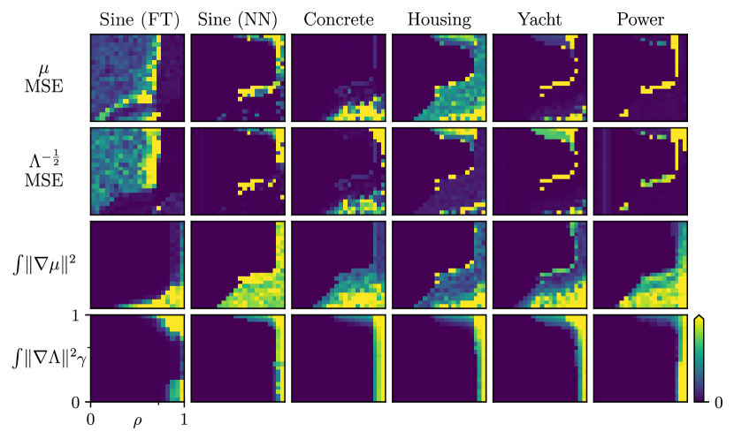
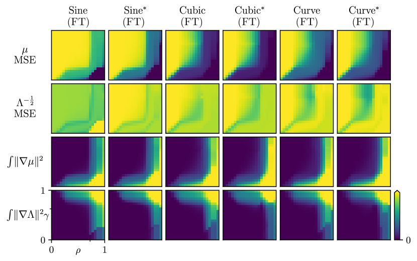
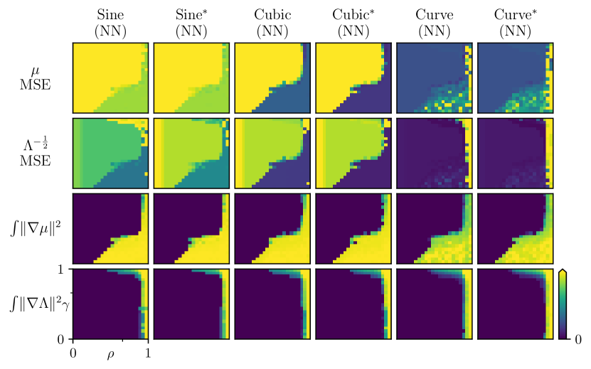
We analyze the effects of regularization on several one-dimensional simulated datasets, standardized versions of the Concrete [Yeh, 2007], Housing [Harrison and Rubinfeld, 1978], Power [Tüfekci, 2014], and Yacht [Gerritsma, 1981] regression datasets from the UC Irvine Machine Learning Repository [Kelly et al., ], and a scalar quantity from the ClimSim dataset [Yu et al., 2023]. We fit neural networks to the simulated and real-world data and additionally solve our FT for the simulated data. Detailed descriptions of the data are included in Section B.1. We present the results for a simulated sinusoidal (Sine) dataset as well as the four UCI regression datasets and have results for the other simulated datasets in Section B.5.
4.1 Qualitative Analysis
Our qualitative analysis aims at understanding architecture-independent aspects of heteroskedastic regression upon varying the regularization strength on the mean and variance functions, resulting in the observation of phase transitions.
Metrics of Interest
We are interested in how well-calibrated the resulting models are as well as how expressive the learned functions are. We compute two types of metrics on our experiments to summarize these properties. Firstly, we consider the mean squared error (MSE). We measure this quantity between predicted mean and target , as well as between predicted standard deviation () and absolute residual . If the mean and standard deviation are well-fit to the data, both of these values should be low. We opt for MSE due to its similarities to variance calibration [Skafte et al., 2019] and expected normalized calibration error [Levi et al., 2022]. Secondly, we evaluate the Dirichlet energy for the FT and its discrete analogue, geometric complexity [Dherin et al., 2022], for neural networks of the learned . As previously mentioned, the Dirichlet energy of a function is defined as . Meanwhile, geometric complexity is . Each quantity captures how expressive a learned function is, with more expressive functions yielding a higher value and is analogous (or equivalent) to the quantity we penalize in the FT setting.
Plot Interpretation
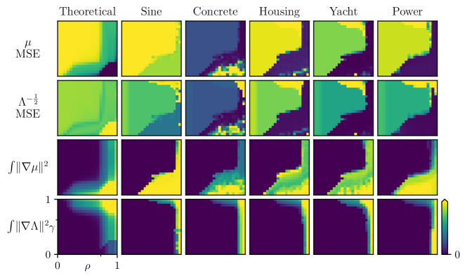
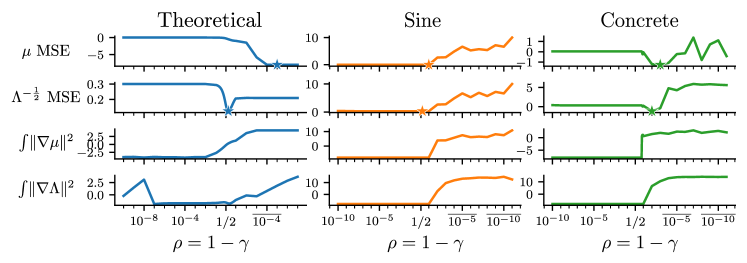
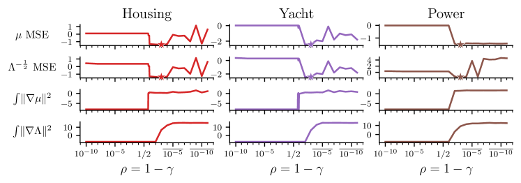
We present summaries of the fitted models in grids with on the -axis and on the -axis in Fig. 2. The far right column () corresponds to MLE solutions. The main focus is on qualitative traits of fits under different levels of regularization and how they behave in a relative sense, rather than a focus on absolute values. Fig. 3 show the summary statistics along the slice where . Zero on these plots corresponds to the upper left corner while one corresponds to the lower right corner.
Observation 1: Our metrics show sharp phase transitions upon varying , as in a physical system. Fig. 2 and Fig. 3 show a sharp transition, both leading to worsening and improving performance when moving along the minor diagonal. In totality, across all metrics, the five regions are apparent. But not all of the regions in Fig. 1 appear in the heatmaps of each metric. For example, region does not always appear in the metrics related to the mean. When using neural networks to approximate and , there are sharper boundaries between phases than in the FT’s numerical solutions. The boundary between and is sharply observed in the plots of . However, in terms of MSE, a smoother transition (i.e., region ) is visible.
Observation 2: The FT insights and observed phases are consistent with the numerically solved FT and the results from fitting neural networks. Thus, our results are not tied to a specific architecture or dataset.
In alignment with our theoretical insights, phases and exhibit consistent behavior across -values (vertical slices in Fig. 2). In the right-hand columns , there is near-perfect matching of the data by the mean function and this is also visible in the lower rows . Within the metrics we assess, the shapes of the regions vary with regularization strength in a similar fashion on all datasets. In the plots of , the region where is flatter covers a larger area compared to the phase diagram showing . That is, for the same proportion of regularization as the mean, the precision remains flatter.
4.2 Quantitative Analysis
Our quantitative analysis aims to demonstrate the practical implications of our qualitative investigations that result in better calibration properties.
Observation 3: We can search along to find a well-calibrated -pair from region .
Our FT indicates that a slice across the minor diagonal of the phase diagram should always cross the region (see Fig. 1). Fig. 3 show that by searching along this diagonal, we indeed find a combination of regularization strengths where both and generalize well to held-out test data. This implies that there is no need to search all of the two-dimensional space, but only a single slice which reduces the number of models to fit from to , where is the number of and values that are tested.
Fig. 3 shows that along the minor diagonal the performance is initially poor, improves, and then drops off again. These shifts from strong to weak performance are sharp. The regularization pairings that result in optimal performance with respect to - and -MSE are near each other along this diagonal for the real-world test data. As the theory predicts, the performance becomes highly variable as we approach the MLE solutions and the FT fails to converge in this region. In practice, we propose searching along this line to find the -combinations that minimize the - and -MSEs and averaging the regularization strengths to fit a model. We compare models chosen by our diagonal line search to two heteroskedastic modeling baselines in Appendix D on the synthetic and UCI datasets as well as a scalar quantity from the ClimSim dataset [Yu et al., 2023]. We present a subset of the results below in Table 2. In most cases the model chosen via the diagonal line search was competitive or better than the baselines.
| Dataset | Ours | -NLL |
| Sine | ||
| MSE | 0.80 ± 0.00 | 4.41 ± 6.90 |
| MSE | 0.80 ± 0.00 | 4.35 ± 6.89 |
| Concrete | ||
| MSE | 0.11 ± 0.02 | 14.99 ± 28.75 |
| MSE | 0.30 ± 0.51 | ± |
| Housing | ||
| MSE | 1.22 ± 0.00 | 8.5 ± |
| MSE | 0.76 ± 0.00 | 8.5 ± |
| Power | ||
| MSE | 0.04± 0.01 | 0.03 ± 0.01 |
| MSE | 0.03 ± 0.01 | 0.04 ± 0.01 |
| Yacht | ||
| MSE | 0.01 ± 0.01 | 3.4 ± 1.9 |
| MSE | 0.01 ± 0.01 | 3.4 ± 1.9 |
| Solar Flux | ||
| MSE | 0.29 ± 0.00 | 0.49 ± 0.16 |
| MSE | 0.12 ± 0.00 | 0.29 ± 0.01 |
5 Related Work
Uncertainty can be divided into epistemic (model) and aleatoric (data) uncertainty [Hüllermeier and Waegeman, 2021], the latter of which can be further divided into homoskedastic (constant over input space) and heteroskedastic (varies over input space). Handling heteroskedastic noise historically has been and continues to be an active area of research in statistics [Huber, 1967, Eubank and Thomas, 1993, Le et al., 2005, Uyanto, 2022] and machine learning [Abdar et al., 2021], but is less common in deep learning [Kendall and Gal, 2017, Fortuin et al., 2022], probably due to pathologies that we analyze in this work. Heteroskedastic noise modeling can be interpreted as reweighting the importance of datapoints during training time, which Wang et al. [2017] show to be beneficial in the presence of corrupted data and Khosla et al. [2022] in active learning.
To the best of our knowledge, Nix and Weigend [1994] were the first to model a mean and standard deviation function with neural networks and Gaussian likelihood. Skafte et al. [2019] suggest changing the optimization loop to train the mean and standard deviation networks separately, treating the standard deviations variationally and integrating them out as Takahashi et al. [2018] does in the context of VAEs, accounting for the location of the data when sampling, and setting a predefined global variance when extrapolating. Stirn and Knowles [2020] also perform amortized VI on the standard deviations and evaluate their model from the perspective of posterior predictive checks. Seitzer et al. [2022] provide an in-depth analysis of the shortcomings of MLE estimation in this setting and adjust the gradients during training to avoid pathological behavior. Stirn et al. [2023] extend the idea of splitting mean and standard deviation network training in a setting where there are several shared layers to learn a representation before emitting mean and standard deviation. Finally, Immer et al. [2023] take a Bayesian approach to the problem and use Laplace approximation on the marginal likelihood to perform empirical Bayes. This allows for regularization to be applied through the prior and for separation of model and data uncertainty. While these works propose practical solutions, in contrast to our work, none of them study the theoretical underpinnings of these pathologies, let alone in a model- or data-agnostic way.
6 Conclusion
We have used field-theoretical tools from statistical physics to derive a nonparametric free energy, which allowed us to produce analytical insights into the pathologies of deep heteroskedastic regression. These insights generalize across models and datasets and provide a theoretical explanation for the need for carefully tuned regularization in these models, due to the presence of sharp phase transitions between pathological solutions.
We have also presented a numerical approximation to this theory, which empirically agrees with neural network solutions to synthetic and real-world data. Insights from the theory have informed a method to tune the regularization to arrive at well-calibrated models more efficiently than would naïvely be the case. Finally, we hope that this work will open an avenue of research for using ideas from theoretical physics to study the behavior of overparameterized models, thus furthering our understanding of otherwise typically unintelligible large models used in AI systems.
Limitations
Our FT and subsequent analysis are restricted to regression problems. From an uncertainty quantification perspective, the models we discuss only account for the aleatoric uncertainty. Though our use of regularizers has a Bayesian interpretation, we are not performing Bayesian inference and do not account for epistemic uncertainty. Solving the FT under a fully Bayesian framework would result in stochastic PDE solutions. We leave analysis of this setting to future work. Additionally, our suggestion to search to find good hyperparameter settings appears to be valid, but requires fitting many models. Ideally, one might hope to use the field theory directly to find optimal regularization settings for real-world models, but our numerical approach is currently not accurate enough for this use case.
Acknowledgements
We acknowledge insightful discussions with Lawrence Saul. Eliot Wong-Toi acknowledges support from the Hasso Plattner Research School at UC Irvine. Alex Boyd acknowledges support from the National Science Foundation Graduate Research Fellowship grant DGE-1839285. Vincent Fortuin was supported by a Branco Weiss Fellowship. Stephan Mandt acknowledges support by the National Science Foundation (NSF) under the NSF CAREER Award 2047418; NSF Grants 2003237 and 2007719, the Department of Energy, Office of Science under grant DE-SC0022331, as well as gifts from Intel, Disney, and Qualcomm.
References
- Abdar et al. [2021] Moloud Abdar, Farhad Pourpanah, Sadiq Hussain, Dana Rezazadegan, Li Liu, Mohammad Ghavamzadeh, Paul Fieguth, Xiaochun Cao, Abbas Khosravi, U. Rajendra Acharya, Vladimir Makarenkov, and Saeid Nahavandi. A review of uncertainty quantification in deep learning: Techniques, applications and challenges. Information Fusion, 76:243–297, December 2021. ISSN 1566-2535. 10.1016/j.inffus.2021.05.008.
- Altland and Simons [2010] Alexander Altland and Ben D. Simons. Condensed Matter Field Theory. Cambridge University Press, Cambridge, 2 edition, 2010. ISBN 978-0-521-76975-4. 10.1017/CBO9780511789984.
- Astivia and Zumbo [2019] Oscar Astivia and Bruno Zumbo. Heteroskedasticity in Multiple Regression Analysis: What it is, How to Detect it and How to Solve it with Applications in R and SPSS. Practical Assessment, Research, and Evaluation, 24(1), November 2019. ISSN 1531-7714. https://doi.org/10.7275/q5xr-fr95.
- Chung and Neiswanger [2021] Youngseog Chung and Willie Neiswanger. Beyond Pinball Loss: Quantile Methods for Calibrated Uncertainty Quantification. 2021.
- Dherin et al. [2022] Benoit Dherin, Michael Munn, Mihaela Rosca, and David G T Barrett. Why neural networks find simple solutions: the many regularizers of geometric complexity. 2022.
- Engel and Dreizler [2011] Eberhard Engel and Reiner M. Dreizler. Density Functional Theory: An Advanced Course. Theoretical and Mathematical Physics. Springer, Berlin, Heidelberg, 2011. ISBN 978-3-642-14089-1 978-3-642-14090-7. 10.1007/978-3-642-14090-7.
- Eubank and Thomas [1993] R. L. Eubank and Will Thomas. Detecting Heteroscedasticity in Nonparametric Regression. Journal of the Royal Statistical Society: Series B (Methodological), 55(1):145–155, 1993. ISSN 2517-6161. 10.1111/j.2517-6161.1993.tb01474.x. _eprint: https://onlinelibrary.wiley.com/doi/pdf/10.1111/j.2517-6161.1993.tb01474.x.
- Fornberg [1988] Bengt Fornberg. Generation of Finite Difference Formulas on Arbitrarily Spaced Grids. Mathematics of Computation, 51:699–706, October 1988.
- Fortuin et al. [2022] Vincent Fortuin, Mark Collier, Florian Wenzel, James Allingham, Jeremiah Liu, Dustin Tran, Balaji Lakshminarayanan, Jesse Berent, Rodolphe Jenatton, and Effrosyni Kokiopoulou. Deep Classifiers with Label Noise Modeling and Distance Awareness. Transactions on Machine Learning Research, 2022.
- Gerritsma [1981] J. Gerritsma. Geometry, resistance and stability of the Delft Systematic Yacht hull series. TU Delft, Faculty of Marine Technology, Ship Hydromechanics Laboratory, Report No. 520-P, Published in: International Shipbuilding Progress, ISP, Delft, The Netherlands, Volume 28, No. 328, also 7th HISWA Symposium, Amsterdam, The Netherlands, 1981.
- Harrison and Rubinfeld [1978] David Harrison and Daniel L Rubinfeld. Hedonic housing prices and the demand for clean air. Journal of Environmental Economics and Management, 5(1):81–102, March 1978. ISSN 0095-0696. 10.1016/0095-0696(78)90006-2.
- Hornik [1991] Kurt Hornik. Approximation capabilities of multilayer feedforward networks. Neural Networks, 4(2):251–257, January 1991. ISSN 0893-6080. 10.1016/0893-6080(91)90009-T.
- Huber [1967] Peter J. Huber. The behavior of maximum likelihood estimates under nonstandard conditions. Proceedings of the Fifth Berkeley Symposium on Mathematical Statistics and Probability, Volume 1: Statistics, 5.1:221–234, January 1967. Publisher: University of California Press.
- Hüllermeier and Waegeman [2021] Eyke Hüllermeier and Willem Waegeman. Aleatoric and epistemic uncertainty in machine learning: an introduction to concepts and methods. Machine Learning, 110(3):457–506, March 2021. ISSN 1573-0565. 10.1007/s10994-021-05946-3.
- Immer et al. [2023] Alexander Immer, Emanuele Palumbo, Alexander Marx, and Julia E Vogt. Effective Bayesian Heteroscedastic Regression with Deep Neural Networks. 2023.
- [16] Markelle Kelly, Rachel Longjohn, and Kolby Nottingham. The UCI Machine Learning Repository. URL https://archive.ics.uci.edu.
- Kendall and Gal [2017] Alex Kendall and Yarin Gal. What Uncertainties Do We Need in Bayesian Deep Learning for Computer Vision? In Advances in Neural Information Processing Systems, volume 30. Curran Associates, Inc., 2017.
- Khosla et al. [2022] Savya Khosla, Chew Kin Whye, Jordan T. Ash, Cyril Zhang, Kenji Kawaguchi, and Alex Lamb. Neural Active Learning on Heteroskedastic Distributions, November 2022. arXiv:2211.00928 [cs].
- Kuleshov et al. [2018] Volodymyr Kuleshov, Nathan Fenner, and Stefano Ermon. Accurate Uncertainties for Deep Learning Using Calibrated Regression. 2018.
- Lakshminarayanan et al. [2017] Balaji Lakshminarayanan, Alexander Pritzel, and Charles Blundell. Simple and Scalable Predictive Uncertainty Estimation using Deep Ensembles. In Neural Information Processing Systems, 2017.
- Landau and Lifshitz [2013] L. D. Landau and E. M. Lifshitz. Statistical Physics: Volume 5. Elsevier, October 2013. ISBN 978-0-08-057046-4.
- Le et al. [2005] Quoc V. Le, Alex J. Smola, and Stéphane Canu. Heteroscedastic Gaussian process regression. In Proceedings of the 22nd international conference on Machine learning - ICML ’05, pages 489–496, Bonn, Germany, 2005. ACM Press. ISBN 978-1-59593-180-1. 10.1145/1102351.1102413.
- Levi et al. [2022] Dan Levi, Liran Gispan, Niv Giladi, and Ethan Fetaya. Evaluating and Calibrating Uncertainty Prediction in Regression Tasks. Sensors (Basel, Switzerland), 22(15):5540, July 2022. ISSN 1424-8220. 10.3390/s22155540. URL https://www.ncbi.nlm.nih.gov/pmc/articles/PMC9330317/.
- Nix and Weigend [1994] D.A. Nix and A.S. Weigend. Estimating the mean and variance of the target probability distribution. In Proceedings of 1994 IEEE International Conference on Neural Networks (ICNN’94), volume 1, pages 55–60 vol.1, June 1994. 10.1109/ICNN.1994.374138.
- Seitzer et al. [2022] Maximilian Seitzer, Arash Tavakoli, Dimitrije Antic, and Georg Martius. ON THE PITFALLS OF HETEROSCEDASTIC UNCERTAINTY ESTIMATION WITH PROBABILISTIC NEURAL NETWORKS. 2022.
- Skafte et al. [2019] Nicki Skafte, Martin Jørgensen, and Søren Hauberg. Reliable training and estimation of variance networks. 2019.
- Stirn and Knowles [2020] Andrew Stirn and David A. Knowles. Variational Variance: Simple, Reliable, Calibrated Heteroscedastic Noise Variance Parameterization, October 2020. arXiv:2006.04910 [cs, stat].
- Stirn et al. [2023] Andrew Stirn, Hans-Hermann Wessels, Megan Schertzer, Laura Pereira, Neville E Sanjana, and David A Knowles. Faithful Heteroscedastic Regression with Neural Networks. 2023.
- Takahashi et al. [2018] Hiroshi Takahashi, Tomoharu Iwata, Yuki Yamanaka, Masanori Yamada, and Satoshi Yagi. Student-t Variational Autoencoder for Robust Density Estimation. In Proceedings of the Twenty-Seventh International Joint Conference on Artificial Intelligence, pages 2696–2702, Stockholm, Sweden, July 2018. International Joint Conferences on Artificial Intelligence Organization. ISBN 978-0-9992411-2-7. 10.24963/ijcai.2018/374.
- Tüfekci [2014] Pınar Tüfekci. Prediction of full load electrical power output of a base load operated combined cycle power plant using machine learning methods. International Journal of Electrical Power & Energy Systems, 60:126–140, September 2014. ISSN 0142-0615. 10.1016/j.ijepes.2014.02.027.
- Uyanto [2022] Stanislaus S. Uyanto. Monte Carlo power comparison of seven most commonly used heteroscedasticity tests. Communications in Statistics - Simulation and Computation, 51(4):2065–2082, April 2022. ISSN 0361-0918. 10.1080/03610918.2019.1692031. Publisher: Taylor & Francis _eprint: https://doi.org/10.1080/03610918.2019.1692031.
- Wang et al. [2017] Yixin Wang, Alp Kucukelbir, and David M. Blei. Robust probabilistic modeling with Bayesian data reweighting. In Proceedings of the 34th International Conference on Machine Learning - Volume 70, ICML’17, pages 3646–3655, Sydney, NSW, Australia, August 2017. JMLR.org.
- Yeh [2007] I-Cheng Yeh. Concrete Compressive Strength, 2007.
- Yu et al. [2023] Sungduk Yu, Walter M. Hannah, Liran Peng, Jerry Lin, Mohamed Aziz Bhouri, Ritwik Gupta, Björn Lütjens, Justus C. Will, Gunnar Behrens, Julius J. M. Busecke, Nora Loose, Charles Stern, Tom Beucler, Bryce E. Harrop, Benjamin R. Hilman, Andrea M. Jenney, Savannah L. Ferretti, Nana Liu, Anima Anandkumar, Noah D. Brenowitz, Veronika Eyring, Nicholas Geneva, Pierre Gentine, Stephan Mandt, Jaideep Pathak, Akshay Subramaniam, Carl Vondrick, Rose Yu, Laure Zanna, Tian Zheng, Ryan P. Abernathey, Fiaz Ahmed, David C. Bader, Pierre Baldi, Elizabeth A. Barnes, Christopher S. Bretherton, Peter M. Caldwell, Wayne Chuang, Yilun Han, Yu Huang, Fernando Iglesias-Suarez, Sanket Jantre, Karthik Kashinath, Marat Khairoutdinov, Thorsten Kurth, Nicholas J. Lutsko, Po-Lun Ma, Griffin Mooers, J. David Neelin, David A. Randall, Sara Shamekh, Mark A. Taylor, Nathan M. Urban, Janni Yuval, Guang J. Zhang, and Michael S. Pritchard. ClimSim: An open large-scale dataset for training high-resolution physics emulators in hybrid multi-scale climate simulators, September 2023. URL http://arxiv.org/abs/2306.08754. arXiv:2306.08754 [physics].
Appendix A Theoretical Details
A.1 Full Functional Derivatives
Our FT is:
and its functional derivatives are
| (11) |
where After setting equal to zero we arrive at
| (12) |
A.2 Proofs
propprop:existence Assuming there exists twice differentiable functions , the following properties hold
-
i
In the absence of regularization (), there are no solutions to the FT.
-
ii
In the absence of data (), there is no unique solution to the FT.
-
iii
There are no valid solutions to the FT if . Some regularization on precision function is needed for a solution to potentially exist.
Proof.
Without loss of generality, we consider a uniform and drop it from the equations.
-
(i)
When the necessary conditions for an optima are
(13) (14) (15) (16) which is a contradiction and there cannot exist that are solutions.
-
(ii)
When the integral we seek to maximize is:
(17) (18) where we . Each term in this integral is non-negative, so the minimum value it could be is zero. Any pair of constant functions will minimize this integral, of which there are infinitely many.
-
(iii)
We return to the -parameterization for this proof. Suppose there is no mean regularization, that is .
(19) From the first condition we see that there must be perfect matching between and since in order to define a valid normal distribution.
(20) (21) Now, note that as ,
(22) but , so the second condition can never be satisfied. Thus, in order for a solution to exist if . These values correspond to .
∎
This proposition implies the existence, or rather the lack thereof of solutions to the FT. Should there be no mean regularization, then there needs to be at least some present for the precision. The theory potentially suggests that the vice versa of this should also guarantee valid solutions (i.e., and ); however, in practice this does not hold true. The reason lies in the stipulation that a.e.
Typically, this condition can be satisfied while still allowing for countably many values of in which . The problem is that we fit models using a finite amount of data. As mentioned previously, we typically minimize the objective function by approximating it using a MC estimate with as samples. An alternative perspective of this decision is that we are actually calculating the expected values exactly with respect to an empirical distribution imposed by : where is the Dirac delta function.333Not to be confused with the functional derivative operator . Because of this, a single value of can possess non-zero measure, thus it only takes a single instance of for the statement a.e. to be false. This, unfortunately, is very likely to happen while solving for . Thus, we can conclude that no matter what, for a valid solution to be guaranteed to exist.
Appendix B Experimental Details
B.1 Datasets
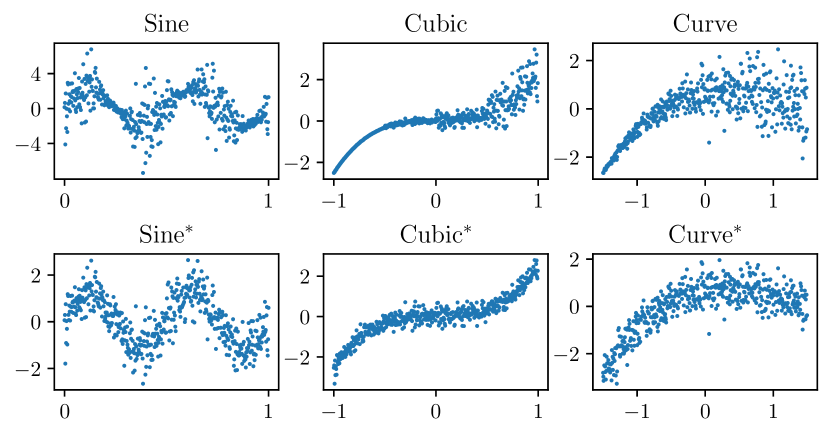
We chose 64 datapoints in each of the simulated datasets. The generating processes for each simulated dataset is included in Table 3 and can be seen in Fig. 4. The homoskedastic data is simulated in the same way, but with . For testing, we simulate a new dataset of 64 datapoints with the same process. Table 4 summarizes the UCI datasets. We provide a description of the ClimSim climate data in Section D.4.
| Dataset | Mean () | Noise Pattern () | Domain |
|---|---|---|---|
| Sine | |||
| Cubic | |||
| Curve |
| Dataset | Train Size | Test Size | Input Dimension |
|---|---|---|---|
| Concrete | 687 | 343 | 8 |
| Housing | 337 | 168 | 13 |
| Power | 6379 | 3189 | 4 |
| Yacht | 204 | 102 | 6 |
B.2 Training Details
We take 22 values of that range from up to on a logit scale for all of the experiments run on neural networks. The exact values were . For the FTs we take 20 values from up to also on a logit scale . This scaling increases the absolute density of points evaluated near the extreme cases of 0 and 1 where the theoretical analysis of the FT focused. The ranges differ slightly due to numerical stability during the fitting. The limiting cases of were omitted for numerical stability and the ranges of values for the FTs vs neural networks vary slightly for the same reason. The values of that were taken along the line were . All experiments were run on Nvidia Quadro RTX 8000 GPUs. Approximately 400 total GPU hours were used across all experiments.
B.3 Metrics
-
•
Geometric complexity: For the one-dimensional datasets the function is evaluated on a dense grid and then the gradients are approximated via finite differences and a trapezoidal approximation to the integral is taken. In the case of the FT, we only assess the function on the solved for, discretized points while with the neural networks we interpolate between points. For the higher-dimensional UCI datasets the gradients are also numerically approximated in the same way but only at the points in the train/test sets.
-
•
MSE: In the fully non-parametric, unconstrained setting, the maximum likelihood estimates at each are and , serving as motivation for checking these differences.
Variability over runs
The experiments were each run six times with different seeds. The standard deviations over the metrics displayed in Fig. 2 are shown in Fig. 5. The Sobolev norms show that there is the most variability in the overfitting regions and parts of . This indicates that the functions themselves vary across runs. However, when turning to quality of fits, the MSEs show a different pattern of regions of instability, and has low variability in terms of actual performance.
B.4 Field Theory
For the discretized field theory we take evenly spaced points on the interval . There are two datapoints placed beyond because the method we use to estimate the gradients requires the datapoints to have left and right neighbors. These datapoints were not included when computing our metrics. Of these 4096 datapoints 64 were randomly selected to be used for training neural networks . The field theory results were consistent across choices of . We present results for in the main paper. We train for epochs and use the Adam optimizer with a basic triangular cycle that scales initial amplitude by half each cycle on the learning rate. The minimum and maximum learning rates were 0.0005 and 0.01. The cycles were 5000 epochs long. We clip the gradients at 1000.
B.5 Simulated Data with Neural Networks
For all of the simulated datasets except for sine we train for epochs and use the Adam optimizer with a basic triangular cycle that scales initial amplitude by half each cycle on the learning rate. The minimum and maximum learning rates were 0.0001 and 0.01. The cycles were 50000 epochs. The first 250000 epochs are only spend on training while the remaining 350000 epochs are spent training both . We clip the gradients at 1000. The training for the sine dataset was the same, except trained for epochs.
B.6 UCI Data with Neural Networks
For the concrete, housing and yacht datasets we train for epochs and use the Adam optimizer with a basic triangular cycle that scales initial amplitude by half each cycle on the learning rate. The minimum and maximum learning rates were 0.0001 and 0.01. The cycles were 50000 epochs. The first 250000 epochs are only spend on training while the remaining 250000 epochs are spent training both . Meanwhile on the power dataset, we had to use minibatching due to the size of the dataset. We used minibatches of 1000 and trained for 50000 total epochs with the first 25000 dedicated solely to and the remainder training both . The same cyclic learning rate was used but with cycle length 5000. We clip the gradients at 1000.
B.7 Practical Suggestion
We can also view the line that we search from the perspective of the parameterization of the regularizers. Let such that
Furthermore, we know that and that . If we are interested in the model settings for for , it then follows that we are equivalently interested in
Appendix C Additional Results
C.1 All Synthetic Dataset Results
Both FT and neural networks were fit to the heteroskedastic and homoskedastic synthetic datasets described in Table 3. The main results for these displayed as phase diagrams of various metrics can be seen in Fig. 6 and Fig. 7 respectively. We largely see the same trends as were exhibited by the real-world datasets seen in Fig. 2.
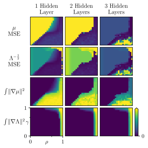
C.2 Effect of Neural Network Size
We used the same training methods to fit models with one and two hidden layers and fit them to the concrete dataset. The results in the phase diagram were consistent with the other experiments, as can be seen in Fig. 8.
Appendix D Comparison to Baselines
We compare the performance of our diagonal search against two baselines, -NLL [Seitzer et al., 2022] and an ensemble of six MLE-fit heteroskedastic regression models [Lakshminarayanan et al., 2017]. We use MSE, MSE, and expected calibration error (ECE) to evaluate the models. In all cases lower values are better. Note that the method of ensembling multiple individual MLE-fit models from Lakshminarayanan et al. [2017] could be implemented on our method or -NLL as well.
D.1 Model Architecture
All (individual) models have the same architecture: fully connected neural networks with three hidden layers of 128 nodes and leaky ReLU activations for the synthetic and UCI datasets and fully connected neural networks with three hidden layers of 256 nodes for the ClimSim data [Yu et al., 2023]. Note that both baselines model the variance while our approach models the precision (inverse-variance). In all cases we use a softplus on the final layer of the variance/precision networks to ensure the output is positive.
For the NLL implementation we take as suggested in Seitzer et al. [2022]. The ensemble method we use fits 6 individual heteroskedastic neural networks and combines their outputs into a mixture distribution that is approximated with a normal distribution. We do not add in adversarial noise as the authors state it does not make a significant difference. We fit six NLL models and six MLE-ensembles.
D.2 Diagonal selection criteria
After conducting our diagonal search we found the model that minimized MSE and the model that minimized MSE on the training data. In some cases these models coincided. We then used the model that was on the midpoint (on a logit scale) of the line between these two models to compare. The results are reported in Table 5. In all cases our method is competitive with or exceeds the performance of these two baselines–particularly on real-world data.
D.3 Training Details
For the baselines, on all of the simulated datasets we train for epochs and use the Adam optimizer with a basic triangular cycle that scales initial amplitude by half each cycle on the learning rate. The minimum and maximum learning rates were 0.0001 and 0.01. The cycles were 50000 epochs. We clip the gradients at 1000. The same optimization scheme is performed for the UCI datasets but for epochs for the Housing, Concrete, and Yacht datasets. The Power dataset was trained for epochs with batches of 1000.
D.4 ClimSim Dataset
The ClimSim dataset [Yu et al., 2023] is a largescale climate dataset. Its input dimension is 124 and output dimension is 128. We use all 124 inputs to model a single output, solar flux. We train on 10,091,520 of the approximately 100 million points for training and we use a randomly selected 7,209 points to evaluate our models.
D.5 Deficiency of ECE
Shortcomings of ECE (in isolation) are well documented [Kuleshov et al., 2018, Levi et al., 2022, Chung and Neiswanger, 2021]. The main issue with ECE is it measures average calibration, while individual calibration is more desirable. On our diagonal search we found that often times the models that achieved the best ECE were those that were severely underfit and belonged to region . In Table 5 we see that the MLE-ensemble is able to achieve low scores while being uncompetitive with respect to the two MSE metrics. The MLE-ensembles were unstable on several of the datasets with respect to the variance network which is consistent with Proposition 1. In particular this can be seen for the synthetic datasets the MSE diverges to infinity.
| Dataset | Ours | -NLL | MLE Ensemble |
|---|---|---|---|
| Metric | Seitzer et al. [2022] | Lakshminarayanan et al. [2017] | |
| Cubic | |||
| ECE | 0.2380 ± 0.03 | 0.2385 ± 0.02 | 0.2411 ± 0.02 |
| MSE | 0.2339 ± 0.01 | 0.1500 ± 0.01 | 1.1809 ± 1.88 |
| MSE | 0.2397 ± 0.02 | 0.1397 ± 0.01 | inf ± nan |
| Curve | |||
| ECE | 0.1804 ± 0.02 | 0.1754 ± 0.02 | 0.2432 ± 0.00 |
| MSE | 0.4318 ± 0.12 | 0.4877 ± 0.16 | 1.0067 ± 0.19 |
| MSE | 0.4655 ± 0.09 | 0.4187 ± 0.20 | inf ± nan |
| Sine | |||
| ECE | 0.2499 ± 0.00 | 0.2082 ± 0.03 | 0.2313 ± 0.05 |
| MSE | 0.7968 ± 0.00 | 4.4107 ± 6.90 | 0.9716 ± 0.06 |
| MSE | 0.7968 ± 0.00 | 4.3524 ± 6.89 | inf ± nan |
| Concrete | |||
| ECE | 0.2471 ± 0.01 | 0.2552 ± 0.00 | 0.0655 ± 0.01 |
| MSE | 0.1055 ± 0.02 | 14.9882 ± 28.75 | 2.2454 ± 1.74 |
| MSE | 0.3028 ± 0.51 | ± | ± |
| Housing | |||
| ECE | 0.0653 ± 0.00 | 0.2631 ± 0.01 | 0.1332 ± 0.02 |
| MSE | 1.2236 ± 0.00 | 851.8968 ± 1985.56 | 155.4494 ± 128.27 |
| MSE | 0.7610 ± 0.00 | 851.8959 ± 1985.56 | 218.8269 ± 195.38 |
| Power | |||
| ECE | 0.2233 ± 0.01 | 0.2370 ± 0.00 | 0.0285 ± 0.01 |
| MSE | 0.0350 ± 0.01 | 0.0313 ± 0.01 | 0.0177 ± 0.00 |
| MSE | 0.0343 ± 0.01 | 0.0360 ± 0.01 | 0.0091 ± 0.00 |
| Yacht | |||
| ECE | 0.3038 ± 0.04 | 0.2882 ± 0.02 | 0.0463 ± 0.02 |
| MSE | 0.0077 ± 0.01 | 34.1239 ± 194.87 | 6.2670 ± 13.96 |
| MSE | 0.0076 ± 0.01 | 34.1237 ± 194.87 | 8.0599 ± 19.18 |
| Solar Flux | |||
| ECE | 0.1503 ± 0.00 | 0.3007 ± 0.00 | 0.1924 ± 0.04 |
| MSE | 0.2887 ± 0.00 | 0.4877 ± 0.16 | 1.0067 ± 0.19 |
| MSE | 0.1175 ± 0.00 | 0.2881 ± 0.01 | ± |