Causal Meta-Analysis by Integrating Multiple Observational Studies with Multivariate Outcomes

Abstract

Integrating multiple observational studies to make unconfounded causal or descriptive comparisons of group potential outcomes in a large natural population is challenging. Moreover, retrospective cohorts, being convenience samples, are usually unrepresentative of the natural population of interest and have groups with unbalanced covariates. We propose a general covariate-balancing framework based on pseudo-populations that extends established weighting methods to the meta-analysis of multiple retrospective cohorts with multiple groups. Additionally, by maximizing the effective sample sizes of the cohorts, we propose a FLEXible, Optimized, and Realistic (FLEXOR) weighting method appropriate for integrative analyses. We develop new weighted estimators for unconfounded inferences on wide-ranging population-level features and estimands relevant to group comparisons of quantitative, categorical, or multivariate outcomes. The asymptotic properties of these estimators are examined, and accurate small-sample procedures are devised for quantifying estimation uncertainty. Through simulation studies and meta-analyses of TCGA datasets, we discover the differential biomarker patterns of the two major breast cancer subtypes in the United States and demonstrate the versatility and reliability of the proposed weighting strategy, especially for the FLEXOR pseudo-population.

Keywords: FLEXOR; Pseudo-population; Retrospective cohort; Unconfounded comparison; Weighting.

1 Introduction

The study of differential patterns of oncogene expression levels across cancer subtypes has aroused great interest because it unveils new tumorigenesis mechanisms and can improve cancer screening and treatment (Kumar et al., 2020). In a multi-site breast cancer study conducted at seven medical centers, including, for example, Memorial Sloan Kettering, Mayo Clinic, and University of Pittsburgh, the goal was to compare the mRNA expression levels of eight targeted breast cancer genes, namely, COL9A3, CXCL12, IGF1, ITGA11, IVL, LEF1, PRB2, and SMR3B (e.g., Zielińska & Katanaev, 2020; Christopoulos et al., 2015) in the disease subtypes infiltrating ductal carcinoma (IDC) and infiltrating lobular carcinoma (ILC), which account for nearly 80% and 10% of breast cancer cases in the United States (U.S.) (Wright, 2022; Tran, 2022). The data reposited at The Cancer Genome Atlas (TCGA) portal (NCI, 2022) include demographic, clinicopathological, and biomarker measurements; some study-specific attributes are summarized in Table 2 of Appendix. Each breast cancer patient’s outcome is a multivariate vector consisting of mRNA expression measurements for these eight genes.

Inference focuses on interpreting biomarker comparisons between the disease subtypes IDC and ILC in the context of a larger disease population in the U.S., e.g., SEER breast cancer patients (Surveillance Research Program, NCI, 2023). The estimands of interest include contrasts and gene-gene pairwise correlations, alongside disease subtype-specific summaries (e.g., means, standard deviations, and medians). Understanding gene expression and co-expression patterns in different subtypes of breast cancer among national-level patients is crucial for developing feasible guidelines for regulating targeted therapies and precision medicine (Schmidt et al., 2016). As revealed by Table 2 of Appendix, naive group comparisons based on the TCGA patient cohorts are severely confounded by the high degree of covariate imbalance between the IDC and ILC subtypes.

More broadly, covariate balance is vitally important in observational studies where interest focuses on unconfounded causal comparisons of group potential outcomes (Robins & Rotnitzky, 1995; Rubin, 2007) in a large natural population such as the U.S. population. The observed populations of convenience samples such as available observational studies are usually unrepresentative of this natural population. Theoretical and simulation studies have demonstrated the conceptual and practical advantages of weighting over other covariate-balancing techniques like matching and regression adjustment (Austin, 2010). As a result, weighting methods have widespread applicability in diverse research areas such as political science, sociology, and healthcare (Lunceford & Davidian, 2004). For analyzing retrospective cohorts consisting of two groups, the propensity score (PS) (Rosenbaum & Rubin, 1983) plays a central role. In these studies, the average treatment effect (ATE) and average treatment effect on the treated group (ATT) are overwhelmingly popular estimands (Robins et al., 2000). The inverse probability weights (IPW) on which these estimators rely may be unstable when some PSs are near 0 or 1 (Li & Li, 2019).

Several researchers have proposed variations of ATE based on truncated subpopulations of scientific or statistical interest (Crump et al., 2006; Li & Greene, 2013). For example, Li et al. (2018) showed that IPWs correspond to a combined pseudo-population and introduced the overlap pseudo-population, wherein the weights minimize the asymptotic variance of the weighted average treatment effect for the overlap pseudo-population (ATO). For single observational studies comprising two or more groups, Li & Li (2019) proposed the generalized overlap pseudo-population that minimizes the sum of asymptotic variances of weighted estimators of pairwise group differences. For observational studies with two groups, Wang & Rosner (2019) developed an integrative approach for Bayesian inferences on ATE.

However, these methods also have several limitations. First, these methods are theoretically guaranteed to be effective for a specific set of outcome types and estimands under certain theoretical conditions (e.g., equal variances of univariate group-specific outcomes). As study endpoints may be continuous, categorical, or multivariate, inference procedures for disparate outcome types have been inadequately explored. Further, scientific interests may necessitate alternative estimands than ATE, ATT or ATO, such as distribution percentiles, standard deviations, pairwise correlations of multivariate outcomes, and unplanned estimands suggested during post hoc analyses. Second, these methods may imply group assignment changes for some subjects that are sometimes difficult to justify for a meaningful, generalizable pseudo-population (Li et al., 2018; Li & Li, 2019). Lastly, very few methods can accommodate integration of multiple observational studies with multiple unbalanced groups as encountered in the TCGA datasets. One potential use of the existing weighing methods to achieve covariate balance is by creating a new categorical variable that combines study and group information. However, it is unclear how to conduct unconfounded group comparisons independent of the “nuisance” study factor. Furthermore, the pseudo-populations generated by this approach are often impractical, and inferential accuracies for common estimands are frequently suboptimal. There is a critical need for developing efficient approaches that enable the integration of multiple observational studies and multiple unbalanced groups and the construction of pseudo-populations that resemble the natural population of interest.

To fill this gap, we extend the propensity score to the observed population multiple propensity score and propose a new class of pseudo-populations and multi-study balancing weights to effectuate data integration and causal meta-analyses. Compared to the existing weighting methods, our work presents two main advances. First, our framework enables unconfounded inferences on a wide variety of population-level group features as well as planned or unplanned estimands relevant to group comparisons. Second, the framework allows us to derive efficient estimators within this proposed family of pseudo-populations. Specifically, by maximizing the effective sample size, we further obtain a FLEXible, Optimized, and Realistic (FLEXOR) weighting method and derive new weighted estimators which are efficient for a variety of quantitative, categorical, and multivariate outcomes, are applicable to different weighting strategies, and effectively utilize multivariate outcome information. For example, the estimators yield efficient estimates of various functionals of group-specific potential outcomes, e.g., contrasts of means and medians, correlations, and percentiles.

The rest of the paper is organized as follows. Section 2 introduces some basic notation, theoretical assumptions, and a general covariate-balancing framework for meta-analysis. We further introduce FLEXOR, an optimized pseudo-population, as its special case. Section 3 develops unconfounded integrative estimators applicable to different weighting methods, estimands, and response types, and establishes asymptotic properties. Section 4 presents the finite sample performance of the proposed methodology, especially when used in conjunction with the FLEXOR weights. Section 5 meta-analyzes the aforementioned TCGA studies and detects differential targeted gene expression and co-expression patterns across the two major breast cancer subtypes in the Unites States. Section 6 concludes with some final remarks.

2 Integration of Observational Studies with Multiple Unbalanced Groups

2.1 Notation and basic assumptions

We aim to compare $K$ subpopulations or groups (e.g., disease subtypes) of participants belonging to a large natural population such as the U.S. patient population. The investigation comprises $J$ observational studies. For $i=1\ldots,N$, let $Z_{i}\in\{1,\ldots,K\}$ denote the group and $S_{i}\in\{1,\ldots,J\}$ denote the observational study. Additionally, there are $p$ covariates shared by all the studies and denoted by $\mathbf{X}_{i}\in\mathcal{X}\subset\mathcal{R}^{p}$ for the $i$th participant. The motivating TCGA database comprises $K=2$ groups corresponding to breast cancer subtype IDC and ILC, and $p=30$ covariates of $N=450$ breast cancer patients in $J=7$ observational studies. The $i$th participant’s potential outcome is $\mathbf{Y}_{i}^{(z)}=(Y_{i1}^{(z)},\ldots,Y_{iL}^{(z)})^{\prime}\in\mathcal{R}^{L}$, i.e., the outcome had the patient belonged to group $z=1,\ldots,K.$ The observed outcome is $\mathbf{Y}_{i}=\mathbf{Y}_{i}^{(Z_{i})}$. In the TCGA example, vectors $\mathbf{Y}^{(1)}_{i}$ and $\mathbf{Y}^{(2)}_{i}$ represent counterfactual mRNA measurements of disease subtypes IDC and ILC on $L=8$ targeted genes, and the observed $\mathbf{Y}_{i}\in\mathcal{R}^{8}$ contains mRNA measurements of breast cancer subtype $Z_{i}$ with which participant $i$ is actually diagnosed.

The participant-specific measurements can be regarded as a random sample from an observed distribution, $[S,Z,\mathbf{X},\mathbf{Y}]_{+}$. Throughout, the symbol $[\cdot]_{+}$ generically represents distributions or densities with respect to the observed population. Extending Rubin (2007) and Imbens (2000b), we assume (A) Stable unit treatment value: given a subject’s covariates, their study and group memberships do not influence the potential outcomes of any other subject; (B) Study-specific weak unconfoundedness: Given study $S$ and covariate vector $\mathbf{X}$, group membership $Z$ is independent of the potential outcomes $\mathbf{Y}^{(1)},\ldots,\mathbf{Y}^{(K)}$; and (C) Positivity: Joint density $[S=z,Z=z,\mathbf{X}=\mathbf{x}]_{+}$ is strictly positive for all $(s,z,\mathbf{x})$. Assumption (B) states that $[\mathbf{Y}^{(z)}\mid S,Z,\mathbf{X}]_{+}=[\mathbf{Y}^{(z)}\mid S,\mathbf{X}]_{+}$. Assumption (C) guarantees that the study and group memberships and covariates do not have deterministic relationships and often holds when $J$ and $K$ are not large.

2.2 A new family of pseudo-populations

We first extend variations of the propensity score (e.g., Rosenbaum & Rubin, 1983) to the observed population multiple propensity score (o-MPS) of the vector $(S,Z)$:

$$\delta_{sz}(\mathbf{x})=\bigl{[}S=s,Z=z\mid\mathbf{X}=\mathbf{x}\bigr{]}_{+}\quad\text{for $(s,z)\in\Sigma$ $\equiv$ $\{1,\ldots,J\}\times\{1,\ldots,K\},$ and $\mathbf{x}\in\mathcal{X}$}.$$

It then follows that the joint density $\bigl{[}S=s,Z=z,\mathbf{X}=\mathbf{x}\bigr{]}_{+}=\delta_{sz}(\mathbf{x})f_{+}(\mathbf{x})$, where $f_{+}(\mathbf{x})=$ $[\mathbf{X}=\mathbf{x}]_{+}$ represents the marginal covariate density in the observed population. As the o-MPS is unknown, we can estimate it by regressing $(S_{i},Z_{i})$ on covariate $\mathbf{x}_{i}$ ($i=1,\ldots,N$). Though propensity scores are often estimated by using parametric (e.g., logistic regression) models, we recommend nonparametric methods that provide more robust and consistent estimates.

Consider a pseudo-population with attributes fully or partially prescribed by the investigator via two probability vectors: (i) relative amounts of information extracted from the studies, quantified by probability tuple $\boldsymbol{\gamma}=(\gamma_{1},\ldots,\gamma_{J})$; and (ii) relative group prevalence, $\boldsymbol{\theta}=(\theta_{1},\ldots,\theta_{K})$. For instance, in the TCGA breast cancer studies, setting $\gamma_{j}=1/7$ extracts equal information from each study, whereas $\boldsymbol{\theta}=$ $(8/9,1/9)$ constrains the pseudo-population to the known U.S. proportions of breast cancer subtypes IDC and ILC (Wright, 2022; Tran, 2022). If some or all components of $\boldsymbol{\gamma}$ or $\boldsymbol{\theta}$ are unknown, subsequent inferences can optimize the pseudo-population over the multiple possibilities for these quantities.

For multiple observational studies, the participant study memberships $S_{1},\ldots,S_{N}$ are primarily influenced by the $J$ study designs and unknown factors driving participation; moreover, study participant characteristics can differ substantially across studies, especially in cancer investigations (Zonderman et al., 2014). To address these issues, we aim to design a pseudo-population for achieving theoretical covariate balance between the $K$ groups. In other words, we construct a pseudo-population wherein the study memberships, the group memberships and patient characteristics are mutually independent, i.e., $S\perp Z\perp\mathbf{X},$ so that

$$\bigl{[}S=s,Z=z,\mathbf{X}=\mathbf{x}\bigr{]}=\gamma_{s}\,\theta_{z}\,f_{\boldsymbol{\gamma},\boldsymbol{\theta}}(\mathbf{x}),\quad\text{for $(s,z,\mathbf{x})\in\Sigma\times\mathcal{X}$.}$$ (1)

Here and hereafter, $[\cdot]$ denotes a distribution or density with respect to the designed pseudo-population, whereas $[\cdot]_{+}$ corresponds to the observed population, as mentioned earlier. Equation (1) further emphasizes that although $S$, $Z$, and $\mathbf{X}$ are independent in the pseudo-population, they may share some distributional parameters. More explicitly, the subscripts of $f_{\boldsymbol{\gamma},\boldsymbol{\theta}}(\mathbf{x})$ emphasize that the pseudo-population density of $\mathbf{X}$ may depend on $\boldsymbol{\gamma}$ and $\boldsymbol{\theta}$.

Next, consider the relationship between the pseudo-population covariate density, $f_{\boldsymbol{\gamma},\boldsymbol{\theta}}(\mathbf{x})$, and the marginal observed covariate density, $f_{+}(\mathbf{x})$. Assuming a common dominating measure for the densities and a common support, $\mathcal{X}$, there exists without loss of generality a positive tilting function (e.g., Li et al., 2018) denoted by $\eta_{\boldsymbol{\gamma},\boldsymbol{\theta}}$ such that $f_{\boldsymbol{\gamma},\boldsymbol{\theta}}(\mathbf{x})\propto\eta_{\boldsymbol{\gamma},\boldsymbol{\theta}}(\mathbf{x})f_{+}(\mathbf{x})$ for all $\mathbf{x}\in\mathcal{X}$. Therefore, $f_{\boldsymbol{\gamma},\boldsymbol{\theta}}(\mathbf{x})=\eta_{\boldsymbol{\gamma},\boldsymbol{\theta}}(\mathbf{x})f_{+}(\mathbf{x})/\mathbb{E}_{+}[\eta_{\boldsymbol{\gamma},\boldsymbol{\theta}}(\mathbf{X})]$ where $\mathbf{X}\sim f_{+}$ and $\mathbb{E}_{+}(\cdot)$ denotes expectations under the observed distribution. Intuitively, high tilting function values correspond to covariate space regions with high pseudo-population weights. Let $\mathcal{S}_{J}$ denote the unit simplex in $\mathcal{R}^{J}$. Different choices of $\boldsymbol{\gamma}\in\mathcal{S}_{J}$, $\boldsymbol{\theta}\in\mathcal{S}_{K}$, and tilting function $\eta_{\boldsymbol{\gamma},\boldsymbol{\theta}}$ identify different pseudo-populations with structure (1).

Balancing weights for integration of multiple studies

To efficiently meta-analyze multiple studies (with $J>1$), we propose the multi-study balancing weight, defined as the ratio of the joint densities with respect to the pseudo-population and observed population. More specifically, for any $(s,z,\mathbf{x})\in\Sigma\times\mathcal{X}$, the multi-study balancing weight

$$\rho(s,z,\mathbf{x})=\frac{\bigl{[}S=s,Z=z,\mathbf{X}=\mathbf{x}\bigr{]}\hfill}{\bigl{[}S=s,Z=z,\mathbf{X}=\mathbf{x}\bigr{]}_{+}}=\frac{\gamma_{s}\,\theta_{z}\,f_{\boldsymbol{\gamma},\boldsymbol{\theta}}(\mathbf{x})}{\delta_{sz}(\mathbf{x})\,f_{+}(\mathbf{x})}=\frac{\gamma_{s}\,\theta_{z}\,\eta_{\boldsymbol{\gamma},\boldsymbol{\theta}}(\mathbf{x})}{\delta_{sz}(\mathbf{x})\,\mathbb{E}_{+}[\eta_{\boldsymbol{\gamma},\boldsymbol{\theta}}(\mathbf{X})]}.$$ (2)

Obviously, $\rho(s,z,\mathbf{x})\bigl{[}S=s,Z=z,\mathbf{X}=\mathbf{x}\bigr{]}_{+}=\bigl{[}S=s,Z=z,\mathbf{X}=\mathbf{x}\bigr{]}$. Hence, the balancing weight serves to redistribute the observed distribution’s relative mass to match that of the pseudo-population. Defining the unnormalized weight function as $\tilde{\rho}(s,z,\mathbf{x})=$ $\gamma_{s}\theta_{z}\eta_{\boldsymbol{\gamma},\boldsymbol{\theta}}(\mathbf{x})/\delta_{sz}(\mathbf{x})$, the empirically normalized balancing weight of the $i$th participant is $\bar{\rho}_{i}=N\tilde{\rho}(s_{i},z_{i},\mathbf{x}_{i})/\sum_{l=1}^{N}\tilde{\rho}(s_{l},z_{l},\mathbf{x}_{l})$. This produces sample weights that sum to $N$ and do not depend on the theoretical expectation $\mathbb{E}_{+}[\eta_{\boldsymbol{\gamma},\boldsymbol{\theta}}(\mathbf{X})]$. For a general pseudo-population (e.g., the FLEXOR pseudo-population introduced in the sequel), the unnormalized weights, even within a study-group combination, may depend on $\boldsymbol{\gamma}$ and $\boldsymbol{\theta}$ through the tilting function. As discussed later, the empirically normalized weights can be utilized to provide unbiased inferences on a variety of potential outcome features for a general pseudo-population.

The proposed pseudo-populations and balancing weights are general, encompassing many well-known weighting methods for single-study settings as special cases. For example, in single studies ($J=1$), suppose we focus on equally prevalent pseudo-population groups ($\theta_{z}=1/K$) in expression (1). A constant tilting function yields IPWs when $K=2$ and generalized IPWs (Imbens, 2000b) when $K>2$. On the other hand, $\eta_{\boldsymbol{\gamma},\boldsymbol{\theta}}(\mathbf{x})=1/\sum_{z}\delta_{z}^{-1}(\mathbf{x})$ produces overlap weights (Li et al., 2018) when $K=2$, and generalized overlap weights (Li & Li, 2019) when $K>2$. Again, if $\eta_{\boldsymbol{\gamma},\boldsymbol{\theta}}(\mathbf{x})=\delta_{z^{\prime}}(\mathbf{x})$ for a group $z^{\prime}$, then the pseudo-population’s covariate density, $f_{\boldsymbol{\gamma},\boldsymbol{\theta}}(\mathbf{x})$, matches the observed covariate density of the group $z^{\prime}$ participants of $J=1$ study.

The choice of different tilting functions in the proposed framework (1) naturally extends several weighting methods designed for single studies to meta-analytical settings. For example, assuming equally weighted studies and equally prevalent groups, i.e., $\gamma_{s}=1/J$ and $\theta_{z}=1/K$, the use of a constant tilting function $\eta_{\boldsymbol{\gamma},\boldsymbol{\theta}}(\mathbf{x})\propto 1$ and $\eta_{\boldsymbol{\gamma},\boldsymbol{\theta}}(\mathbf{x})=1/\sum\sum_{s,z}\delta_{sz}^{-1}(\mathbf{x})$, respectively, produces extensions of the combined (Li et al., 2018) and generalized overlap (Li & Li, 2019) pseudo-populations that are appropriate for meta-analyzing multiple studies with multiple groups. We refer to these proposed pseudo-populations as the integrative combined (IC) and integrative generalized overlap (IGO) pseudo-populations, respectively. Similarly, for a fixed group $z^{\prime}$, the tilting function $\eta_{\boldsymbol{\gamma},\boldsymbol{\theta}}(\mathbf{x})=\sum_{s}\delta_{sz^{\prime}}(\mathbf{x})$ gives a pseudo-population whose marginal covariate density equals the observed covariate density of group $z^{\prime}$ participants irrespective of their study memberships. Given the availability of different tilting functions, an important question arises: which choice is optimal and in what sense? We address this below.

Effective sample size

A widely used measure of a pseudo-population’s inferential accuracy is the effective sample size (ESS), $\mathcal{Q}(\boldsymbol{\gamma},\boldsymbol{\theta},\eta_{\boldsymbol{\gamma},\boldsymbol{\theta}})=N/\bigl{[}1+\text{Var}_{+}\bigl{\{}\rho(S,Z,\mathbf{X})\bigr{\}}\bigr{]}=N/\mathbb{E}_{+}\bigl{[}\rho^{2}(S,Z,\mathbf{X})\bigr{]},$ which relies on the second moment (provided it exists) of the balancing weights in the observed population (e.g., McCaffrey et al., 2013). The ESS is asymptotically equivalent to the sample ESS, $\tilde{\mathcal{Q}}(\boldsymbol{\gamma},\boldsymbol{\theta},\eta_{\boldsymbol{\gamma},\boldsymbol{\theta}})=N^{2}/\sum_{i=1}^{n}\bar{\rho}_{i}^{2}$. Informally, the ESS is the hypothetical sample size from the pseudo-population containing the same information as $N$ samples from the observed population, and it is always less than $N$ unless the pseudo-population and observed population are identical.

An optimized case: FLEXOR pseudo-population.

We propose FLEXOR as a member of pseudo-population family (1) that maximizes the ESS or minimizes the variation of the balancing weights, subject to any problem-dictated constraints on the vectors $\boldsymbol{\gamma}$ and $\boldsymbol{\theta}$. That is, if the triplet $(\breve{\boldsymbol{\gamma}},\breve{\boldsymbol{\theta}},\breve{\eta}_{\breve{\boldsymbol{\gamma}},\breve{\boldsymbol{\theta}}})$ identifies the FLEXOR pseudo-population and the investigation stipulates that $(\boldsymbol{\gamma},\boldsymbol{\theta})$ belong to a subset, $\Upsilon$, of $\mathcal{S}_{J}\times\mathcal{S}_{K}$, then $\mathcal{Q}(\breve{\boldsymbol{\gamma}},\breve{\boldsymbol{\theta}},\breve{\eta}_{\breve{\boldsymbol{\gamma}},\breve{\boldsymbol{\theta}}})=\sup_{(\boldsymbol{\gamma},\boldsymbol{\theta})\in\Upsilon}\sup_{\eta_{\boldsymbol{\gamma},\boldsymbol{\theta}}}\mathcal{Q}(\boldsymbol{\gamma},\boldsymbol{\theta},\eta_{\boldsymbol{\gamma},\boldsymbol{\theta}})$.

A two-step procedure for constructing the FLEXOR pseudo-population

Starting with an initial $(\boldsymbol{\gamma},\boldsymbol{\theta})\in\Upsilon$, we iteratively perform the following steps until convergence:

• Step I  For a fixed $(\boldsymbol{\gamma},\boldsymbol{\theta})$, maximize $\mathcal{Q}(\boldsymbol{\gamma},\boldsymbol{\theta},\eta_{\boldsymbol{\gamma},\boldsymbol{\theta}})$ over all tilting functions, $\eta_{\boldsymbol{\gamma},\boldsymbol{\theta}}$. This gives the best fixed-$(\boldsymbol{\gamma},\boldsymbol{\theta})$ pseudo-population, identified by the triplet $(\boldsymbol{\gamma},\boldsymbol{\theta},\tilde{\eta}_{\boldsymbol{\gamma},\boldsymbol{\theta}})$. The analytical form of $\tilde{\eta}_{\boldsymbol{\gamma},\boldsymbol{\theta}}$ is given in Theorem 2.1 below. Set function $\eta=\tilde{\eta}_{\boldsymbol{\gamma},\boldsymbol{\theta}}$.

• Step II  For a fixed tilting function $\eta$, maximize $\mathcal{Q}(\boldsymbol{\gamma},\boldsymbol{\theta},\eta)$ over all $(\boldsymbol{\gamma},\boldsymbol{\theta})\in\Upsilon$ to obtain the best fixed-$\eta$ pseudo-population, identified by the triplet $(\tilde{\boldsymbol{\gamma}},\tilde{\boldsymbol{\theta}},\eta)$. This parametric maximization over $\Upsilon\subset\mathcal{S}_{J}\times\mathcal{S}_{K}$ can be quickly performed in R using the optim function or by Gauss-Seidel or Jacobi algorithms. Set $(\boldsymbol{\gamma},\boldsymbol{\theta})=(\tilde{\boldsymbol{\gamma}},\tilde{\boldsymbol{\theta}})$.

In our experience, convergence is attained within only a few iterations. The converged pseudo-population with the largest ESS yields the FLEXOR pseudo-population. The following theorem gives the analytical expression for the global maximum of $\mathcal{Q}(\boldsymbol{\gamma},\boldsymbol{\theta},\eta_{\boldsymbol{\gamma},\boldsymbol{\theta}})$ in Step I. See Appendix for the proof.

Theorem 2.1.

Suppose probability vectors $\boldsymbol{\gamma}$ and $\boldsymbol{\theta}$ have strictly positive elements and are held fixed. Let $\boldsymbol{\Xi}$ be the set of tilting functions for which the ESS, $\mathcal{Q}(\boldsymbol{\gamma},\boldsymbol{\theta},\eta_{\boldsymbol{\gamma},\boldsymbol{\theta}})$, of pseudo-population (1) is finite. Maximizing $\mathcal{Q}(\boldsymbol{\gamma},\boldsymbol{\theta},\eta_{\boldsymbol{\gamma},\boldsymbol{\theta}})$ over all tilting functions $\eta_{\boldsymbol{\gamma},\boldsymbol{\theta}}\in\boldsymbol{\Xi}$, the optimal fixed-$(\boldsymbol{\gamma},\boldsymbol{\theta})$ pseudo-population’s tilting function, denoted by $\tilde{\eta}_{\boldsymbol{\gamma},\boldsymbol{\theta}}$, has the expression:

$$\tilde{\eta}_{\boldsymbol{\gamma},\boldsymbol{\theta}}(\mathbf{x})=\biggl{(}\sum_{s=1}^{J}\sum_{z=1}^{K}\frac{\gamma_{s}^{2}\theta_{z}^{2}}{\delta_{sz}(\mathbf{x})}\biggr{)}^{-1},\quad\text{ $\mathbf{x}\in\mathcal{X}$.}$$ (3)

The unnormalized weight function for the optimal fixed-$\boldsymbol{\gamma}$ pseudo-population is then

$$\tilde{\rho}(s,z,\mathbf{x})=\frac{1}{\gamma_{s}\theta_{z}}\biggl{(}\frac{\gamma_{s}^{2}\theta_{z}^{2}/\delta_{sz}(\mathbf{x})}{\sum_{t=1}^{J}\sum_{u=1}^{K}\gamma_{t}^{2}\theta_{u}^{2}/\delta_{tu}(\mathbf{x})}\biggr{)},\qquad\text{for $(s,z)\in\Sigma$ and $\mathbf{x}\in\mathcal{X}$.}$$ (4)

The optimal fixed-$(\boldsymbol{\gamma},\boldsymbol{\theta})$ pseudo-population’s balancing weights, evaluated as in (2), are uniformly bounded for $(s,z,\mathbf{x})$ belonging to $\Sigma\times\mathcal{X}$. The ESS of the optimal fixed-$\boldsymbol{\gamma}$ pseudo-population is $N\mathbb{E}_{+}\bigl{[}\tilde{\eta}_{\boldsymbol{\gamma},\boldsymbol{\theta}}(\mathbf{X})\bigr{]}$ with the expectation taken over $\mathbf{X}\sim f_{+}(\mathbf{x})$, the observed population’s covariate density.

3 Meta-analyses of Group Potential Outcomes

Causal meta-analyses generally follow a two-stage inferential procedure (e.g., Rubin, 2008; Austin & Stuart, 2015). In Stage 1, the “outcome free” analysis only utilizes covariate information to estimate the propensity scores, as done in Section 2. In Stage 2, conditional on the estimated o-MPS and pseudo-population, the procedure makes unconfounded comparisons of group potential outcomes via estimands such as ATT or ATE. We follow this basic strategy, except that for any known pseudo-population belonging to family (1), we modify Stage 2 to accommodate wide-ranging group-level features of the endpoints using the available multivariate outcome information. For notational convenience, we conflate the estimated and true o-MPS in the sequel.

Suppose potential outcome vectors $\mathbf{Y}^{(1)},\ldots,$ $\mathbf{Y}^{(K)}$ have a common support, $\mathcal{Y}\subset\mathcal{R}^{L}$. To ensure that the stable unit treatment value, study-specific weak unconfoundedness, and positivity assumptions for the observed population also hold for the pseudo-population, we assume identical conditional distributions in the observed population and pseudo-population for the potential outcomes:

$$[\mathbf{Y}^{(z)}\mid S,Z,\mathbf{X}]=[\mathbf{Y}^{(z)}\mid S,Z,\mathbf{X}]_{+}\quad\text{for group $z=1,\ldots,K$},$$ (5)

where we recall that $[\cdot]_{+}$ and $[\cdot]$ denote the observed and pseudo-population population densities, respectively. Unlike the observed population, the covariate-balanced pseudo-population entails $[\mathbf{Y}\mid Z=z]=[\mathbf{Y}^{(z)}]$, enabling us to construct weighted estimators of various features of the pseudo-population potential outcomes.

Let $\mathbb{E}[\cdot]$ denote expectations with respect to the pseudo-population. Let $\Phi_{1},\ldots,\Phi_{M}$ be measurable real-valued functions having domain $\mathcal{Y}$. We wish to infer pseudo-population means of transformed potential outcomes, $\mathbb{E}[\Phi_{1}(\mathbf{Y}^{(z)})],\ldots,\mathbb{E}[\Phi_{M}(\mathbf{Y}^{(z)})]$ for $z=1,\ldots,K$. Appropriate choices of $\Phi_{m}$ correspond to pseudo-population inferences about group-specific marginal means, medians, variances, and CDFs of potential outcome components. Equivalently, writing $\mathbf{\Phi}(\mathbf{Y}^{(z)})=\bigl{(}\Phi_{1}(\mathbf{Y}^{(z)}),\ldots,\Phi_{M}(\mathbf{Y}^{(z)})\bigr{)}^{\prime}\in\mathcal{R}^{M}$, the inferential focus is the vector, $\boldsymbol{\lambda}^{(z)}=$ $\mathbb{E}[\mathbf{\Phi}(\mathbf{Y}^{(z)})]$.

For real-valued measurable functions $\psi$ with domain $\mathcal{R}^{M}$, we estimate $\psi(\boldsymbol{\lambda}^{(z)})$. For example, if the first two components of $\mathbf{Y}^{(z)}$ are quantitative, then defining $\Phi_{1}(\mathbf{Y}^{(z)})=Y_{1}^{(z)}$, $\Phi_{2}(\mathbf{Y}^{(z)})=Y_{2}^{(z)}$, $\Phi_{3}(\mathbf{Y}^{(z)})=Y_{1}^{(z)}Y_{2}^{(z)}$, and $\psi(t_{1},t_{2},t_{3})=t_{3}-t_{1}t_{2}$, we obtain $\psi(\boldsymbol{\lambda}^{(z)})=\text{cov}(Y_{1}^{(z)},Y_{2}^{(z)})$ as the pseudo-population covariance of $Y_{1}^{(z)}$ and $Y_{2}^{(z)}$ in the $z$th group. The pseudo-population correlation of pairwise components of $\mathbf{Y}^{(z)}$ can be estimated from estimates of the covariance and standard deviations, as in the motivating breast cancer studies, where the goal is to estimate the pairwise correlations of the eight targeted genes in groups $z\in\{1,2\}$ (i.e., IDC and ILC subtypes).

Using the empirically normalized balancing weights $\bar{\rho}_{1},\ldots,\bar{\rho}_{N}$ [defined underneath (2)] of a pseudo-population, we estimate $\mathbb{E}[\mathbf{\Phi}(\mathbf{Y}^{(z)})]$ by

$$\mathbf{\bar{\Phi}}_{z}=\frac{1}{N\theta_{z}}\sum_{i=1}^{N}\bar{\rho}_{i}\,\mathbf{\Phi}(\mathbf{Y}_{i})\,\mathcal{I}(Z_{i}=z).$$ (6)

The following theorem and corollaries study asymptotic properties of random vector $\mathbf{\bar{\Phi}}_{z}$ as an estimator of multivariate feature $\mathbb{E}[\mathbf{\Phi}(\mathbf{Y}^{(z)})]$. The proofs are available in the Appendix.

Theorem 3.1.

Let $\mathbb{E}_{+}[\cdot]$ and $\mathbb{E}[\cdot]$ respectively denote expectations with respect to the observed population and a pseudo-population of the form (1). Let observed probability $P_{+}[S=s]$ be strictly positive for study $s=1,\ldots,J$. Suppose the conditional distributions of the potential outcomes are weakly unconfounded, as described in Section 2, and satisfy assumption (5). Suppose $\mathbb{E}_{+}[w^{2}_{\boldsymbol{\Phi}}(\mathbf{X})]$ is finite. For $m=1,\ldots,M$, let $\Phi_{m}$ be a measureable real-valued function with domain $\mathcal{Y}$ such that $\mathbb{E}_{+}[w_{\boldsymbol{\Phi}}(\mathbf{X})\Phi_{m}(\mathbf{Y})]$ is finite. Interest focuses on the pseudo-population moment, $\mathbb{E}[\mathbf{\Phi}(\mathbf{Y}^{(z)})]$, also denoted by vector $\boldsymbol{\lambda}^{(z)}=(\lambda_{1}^{(z)},\ldots,\lambda_{M}^{(z)})^{\prime}$. Estimator $\mathbf{\bar{\Phi}}_{z}$ defined in (6) has the following properties as $N\to\infty$:

1. Consistency: $\mathbf{\bar{\Phi}}_{z}\stackrel{{\scriptstyle p}}{{\to}}\boldsymbol{\lambda}^{(z)}$.

2. Asymptotic normality: For $m=1,\ldots,M$, suppose observed moment $\mathbb{E}_{+}[w^{2}_{\boldsymbol{\Phi}}(\mathbf{X})\Phi_{m}^{2}(\mathbf{Y})]$ is finite. Then $\sqrt{N}\biggl{(}\mathbf{\bar{\Phi}}_{z}-\boldsymbol{\lambda}^{(z)}\biggr{)}\stackrel{{\scriptstyle d}}{{\to}}N_{M}\bigl{(}\mathbf{0},\boldsymbol{\Sigma}^{(z)}\bigr{)},$ where, for $m,m^{\prime}=1,\ldots,M$, the $(m,m^{\prime})$th element of matrix $\boldsymbol{\Sigma}^{(z)}$ is

   $$\bigl{(}\sigma_{mm^{\prime}}^{(z)}\bigr{)}^{2}=\frac{1}{\theta_{z}^{2}}\mathbb{E}_{+}\biggl{[}\rho^{2}(S,Z,\mathbf{X})\biggl{(}\Phi_{m}(\mathbf{Y})\,\mathcal{I}(Z=z)-\theta_{z}\lambda_{m}^{(z)}\biggr{)}\biggl{(}\Phi_{m^{\prime}}(\mathbf{Y})\,\mathcal{I}(Z=z)-\theta_{z}\lambda_{m^{\prime}}^{(z)}\biggr{)}\biggr{]}.$$ (7)

3. A consistent estimator of matrix $\boldsymbol{\Sigma}^{(z)}$ is $\hat{\boldsymbol{\Sigma}}^{(z)}$ with the $(m,m^{\prime})$th element being

   $$\bigl{(}s_{mm^{\prime}}^{(z)}\bigr{)}^{2}=\frac{1}{N\theta_{z}^{2}}\sum_{i=1}^{N}\bar{\rho}_{i}^{2}\biggl{(}\Phi_{m}(\mathbf{Y}_{i})\,\mathcal{I}(Z_{i}=z)-\theta_{z}\bar{\Phi}_{zm}\biggr{)}\biggl{(}\Phi_{m^{\prime}}(\mathbf{Y}_{i})\,\mathcal{I}(Z_{i}=z)-\theta_{z}\bar{\Phi}_{zm^{\prime}}\biggr{)},$$

   for $m,m^{\prime}=1,\ldots,M$, where the $m$th component of vector $\mathbf{\bar{\Phi}}_{z}$ is denoted by $\bar{\Phi}_{zm}$. If $\boldsymbol{\Sigma}^{(z)}$ is invertible, then $\sqrt{N}\hat{\mathbf{A}}_{z}\biggl{(}\mathbf{\bar{\Phi}}_{z}-\boldsymbol{\lambda}^{(z)}\biggr{)}\stackrel{{\scriptstyle d}}{{\to}}N_{M}\bigl{(}\mathbf{0},\mathbf{I}\bigr{)},$ where $\hat{\mathbf{A}}_{z}=\bigl{(}\hat{\boldsymbol{\Sigma}}^{(z)}\bigr{)}^{-1/2}$ if $\hat{\boldsymbol{\Sigma}}^{(z)}$ is invertible, and defined arbitrarily otherwise.

Corollary 3.1.1.

For the FLEXOR pseudo-population, the sufficient conditions are considerably simplified if its study weights, $\breve{\gamma}_{s}$, are strictly positive. Assume the observed probability $P_{+}[S=s]$ of each study is also positive, and that the potential outcomes are conditionally weakly unconfounded and satisfy assumption (5). Then Parts 1-3 of Theorem 3.1 hold, provided the observed moment $\mathbb{E}_{+}[\Phi_{m}^{2}(\mathbf{Y})]$ is finite for $m=1,\ldots,M$.

Corollary 3.1.2.

Let $\psi$ be a real-valued differentiable function with domain $\mathcal{R}^{M}$. Let $\nabla\psi(\boldsymbol{\lambda})=\partial\psi(\boldsymbol{\lambda})/\partial\boldsymbol{\lambda}$ denote the gradient vector of length $M$ at $\boldsymbol{\lambda}$. With matrix $\boldsymbol{\Sigma}^{(z)}$ defined as in (7), suppose the scalar $\nabla^{\prime}\psi(\boldsymbol{\lambda}^{(z)})\,\boldsymbol{\Sigma}^{(z)}\,\nabla\psi(\boldsymbol{\lambda}^{(z)})$ is positive at $\boldsymbol{\lambda}^{(z)}=\mathbb{E}[\mathbf{\Phi}(\mathbf{Y}^{(z)})]$. Define $\hat{\tau}_{z}=$ $\nabla^{\prime}\psi(\mathbf{\bar{\Phi}}_{z})\,\hat{\boldsymbol{\Sigma}}^{(z)}\,\nabla\psi(\mathbf{\bar{\Phi}}_{z})$ if the right hand quantity is positive; otherwise, let $\hat{\tau}_{z}$ be an arbitrary number. Then $\psi(\mathbf{\bar{\Phi}}_{z})$ is a consistent and asymptotically normal estimator of $\psi(\boldsymbol{\lambda}^{(z)})$: $\frac{\sqrt{N}}{\hat{\tau}_{z}}\biggl{(}\psi(\mathbf{\bar{\Phi}}_{z})-\psi(\boldsymbol{\lambda}^{(z)})\biggr{)}\stackrel{{\scriptstyle d}}{{\to}}N\bigl{(}0,1\bigr{)}.$

Remark. Theorem 3.1 and its corollaries summarize several noteworthy features of estimator (6) and its FLEXOR version: (i) the estimator is consistent and asymptotically multivariate normal, justifying the use of normal distributions for large sample inferences; (ii) they are applicable to the balancing weights of any pseudo-populations, including IC, IGO, and FLEXOR weights; (iii) they generalize weighted estimators of the average controlled difference (ACD) (Hirano & Imbens, 2001; Li et al., 2018) and plug-in sample moment estimators (Li & Li, 2019) to multiple groups and studies, while accommodating mixed-type multivariate outcomes, (iv) like other causal inference methods, they condition on the estimated propensity scores and pseudo-populations from Stage 1; by contrast, the bootstrap methods discussed below account for any additional sources of variation, including the estimated PSs, and (v) they exploit known or researcher-supplied information about the group proportions of the pseudo-population; as previously mentioned, the FLEXOR weights typically set $\theta_{z}$ equal to the known group prevalences of the larger population. By contrast, $\theta_{z}=1/K$ for most other weighting methods.

Group comparisons

Consider estimation of the pseudo-population moment $\mathbb{E}[\Phi_{m}(\mathbf{Y}^{(z)})]$ using $\bar{\Phi}_{zm}$. Applying standard results (e.g., Johnson et al., 2002, Chapter 5), we can construct approximate $100(1-\alpha)$% confidence intervals simultaneously for all possible linear combinations of $\mathbb{E}[\Phi_{m}(\mathbf{Y}^{(1)})],\ldots,$ $\mathbb{E}[\Phi_{m}(\mathbf{Y}^{(K)})]$. In particular, for large $N$, using the $m$th diagonal element of $\hat{\boldsymbol{\Sigma}}^{(z)}$ defined in Theorem 3.1, the interval $\sum_{z=1}^{K}a_{z}\,\bar{\Phi}_{zm}\pm\sqrt{\chi^{2}_{K}(\alpha)\sum_{z=1}^{K}a_{z}^{2}\,\bigl{(}s_{mm}^{(z)}\bigr{)}^{2}/N}$ contains $\sum_{z=1}^{K}a_{z}\,\mathbb{E}[\Phi_{m}(\mathbf{Y}^{(z)})]$ with approximate probability $(1-\alpha)$ simultaneously for all scalars $a_{1},\ldots,a_{K}$.

Various pseudo-population features can then be compared between the $K$ groups. Writing $\lambda^{(zm)}=\mathbb{E}[Y_{m}^{(z)}]$, we could estimate contrasts such as $\lambda^{(1m)}-\lambda^{(2m)}$ (e.g., average difference between the $m$th gene’s mRNA expression levels for IDC and ILC breast cancer patients) and, when $K>2$, $\lambda^{(1m)}-\frac{1}{K-1}\sum_{z=2}^{K}\lambda^{(zm)}$ (e.g., for the $m$th gene, average difference between the mRNA expression levels for a reference group and the average of the other groups). We could also estimate ratios of means such as $\lambda^{(zm)}/\lambda^{(1m)}$, ratios of mean differences such as $\bigl{(}\lambda^{(3m)}-\lambda^{(1m)}\bigr{)}/\bigl{(}\lambda^{(2m)}-\lambda^{(1m)}\bigr{)}$, group-specific standard deviations, percentiles, ratios of medians, and ratios of coefficients of variation. Under mild conditions, these estimators are consistent and asymptotically normal, and their asymptotic variances are available by applying Corollary 3.1.2 and the delta method.

If $N_{z}$ is small for some groups, such as rare or undersampled treatments, the asymptotic confidence intervals for $\beta$, which generically denotes a real-valued pseudo-population feature of interest, may have coverage away from the nominal levels. We then propose to employ nonparametric bootstrap methods (Efron & Tibshirani, 1994; Bickel & Freedman, 1981; Van der Vaart, 2000) to estimate the standard error $\tau_{\beta}$ of estimator $\hat{\beta}$ as follows. For patient $i=1,\ldots,N$, let $\boldsymbol{\xi}_{i}=(\boldsymbol{\varphi}_{i},\mathbf{x}_{i},y_{i})$. Using the empirically normalized balancing weights, we draw $B$ bootstrap samples of size $N$ from the mixture distribution, $F^{*}=\frac{1}{N}\sum_{i=1}^{N}\zeta_{\boldsymbol{\xi}_{i}}$, where $\zeta_{\boldsymbol{\xi}}$ represents a point mass at $\boldsymbol{\xi}$. Denote by $\boldsymbol{\xi}_{i}^{(b)}$ the $t$th draw in the $b$th bootstrap sample, so that $\boldsymbol{\xi}_{t}^{(b)}\stackrel{{\scriptstyle iid}}{{\sim}}F^{*}$. Let $\hat{\beta}^{(b)}$ be the weighted estimate of feature $\beta$ based on the $b$th bootstrap sample. Then a bootstrap estimate of standard error $\tau_{\beta}$ is

$$\hat{\tau}_{\beta}=\left\{\frac{1}{B-1}\sum_{b=1}^{B}\biggl{(}\hat{\beta}^{(b)}-\bar{\beta}\biggr{)}^{2}\right\}^{1/2},$$

where $\bar{\beta}=\sum_{b=1}^{B}\hat{\beta}^{(b)}/B$. For a fixed sample size $N$, we have $\hat{\tau}_{\beta}\stackrel{{\scriptstyle p}}{{\to}}\tau_{\beta}$ as $B\to\infty$. For large $B$, $\hat{\tau}_{\beta}$ can be used to construct 95% confidence intervals for $\beta$. Alternatively, the 2.5th and 97.5th percentiles of $\hat{\beta}^{(1)},\ldots,\hat{\beta}^{(B)}$ give distribution-free CIs for pseudo-population feature $\beta$.

4 Simulation Study

We used simulated datasets to evaluate different weighting strategies for inferring the population-level features of two subject groups and assessed the accuracy of the Section 3 asymptotic variance expression for the mean group differences. Mimicking the motivating TCGA breast cancer studies, we simulated $R=500$ independent datasets, each consisting of $J=4$ observational studies, $K=2$ groups, and $L=1$ (i.e., univariate) uncensored outcomes for $\tilde{N}$ subjects whose covariate vectors were sampled with replacement from the $N=450$ TCGA breast cancer patients. We first took $\tilde{N}=450$ subjects in two scenarios characterized by different covariate similarity degrees between the $JK=8$ study-group combinations. We then applied the Section 3 procedure to meta-analyze the four studies in each artificial dataset. Additionally, by increasing $\tilde{N}$ from $125$, to $250$, and then to $450$ subjects, we compared the asymptotic and bootstrap-based variances of the ATE, $\lambda^{(1)}-\lambda^{(2)}$, where $\lambda^{(z)}=\mathbb{E}[Y^{(z)}]$.

To create artificial datasets with realistic associations between the studies, groups, and covariates, we first inferred $\hat{\delta}_{sz}(\mathbf{x})$, the estimated o-MPS, in the motivating TCGA datasets using random forests (Breiman, 2001). The estimated o-MPS was the basis of a realistic mechanism for generating the $\tilde{N}$ study and group allocations in Step 2 below. Next, each covariate was designated as either a non-predictor, linear, or quadratic outcome predictor: for covariate $t=1,\ldots,p$, we independently generated category $A_{t}\in\{0,1,2\}$ with probabilities $0.5$, $0.25$, and $0.25$, respectively, signifying that the $t$th covariate is a non-predictor, linear and quadratic predictor. Let the $\tilde{A}=\sum_{t}^{p}\mathcal{I}(A_{t}>0)$ predictors be arranged in an $N\times\tilde{A}$ matrix, $\mathbf{Q}$, with rows $\mathbf{q}_{1}^{\prime},\ldots,\mathbf{q}_{N}^{\prime}$. We subsequently used this predictor matrix to generate the $\tilde{N}$ responses in each of the $R=500$ datasets in Step 3 below. Specifically, using matrix $\mathbf{Q}$, and for artificial dataset $r=1,\ldots,500$, we generated the data as follows:

1. Covariates and predictor matrix rows  For subject $i=1,\ldots,\tilde{N}$, covariate vector $\tilde{\mathbf{x}}_{i}^{(r)}=(\tilde{x}_{i1}^{(r)},\ldots,\tilde{x}_{ip}^{(r)})^{\prime}$ and predictor matrix row $\mathbf{q}_{ir}^{\prime}$ were jointly sampled with replacement from the actual covariates of the $N$ patients of the TCGA dataset and the corresponding rows of matrix $\mathbf{Q}$. For the $r$th dataset, let the sampled rows of the matrix $\mathbf{Q}$, denoted by $\mathbf{q}_{1r}^{\prime},\ldots,\mathbf{q}_{\tilde{N}r}^{\prime}$, be stacked to construct the $\tilde{N}\times\tilde{A}$ matrix, $\mathbf{Q}^{(r)}$.

2. Study and group memberships  Study $s_{i}^{(r)}$ and group $z_{i}^{(r)}$ were generated as follows:

   1. Similarity scenarios  For a similarity parameter $\pi>0$, and independently for $i=1,\ldots,\tilde{N}$, we generated $\boldsymbol{\delta}_{r}^{(i)}(\mathbf{x}_{i})=\bigl{(}\delta_{11r}^{(i)}(\mathbf{x}_{i}),\ldots,\delta_{JKr}^{(i)}(\mathbf{x}_{i})\bigr{)}$, the o-MPS vector of the $i$th subject, as $\boldsymbol{\delta}_{r}^{(i)}(\mathbf{x}_{i})\sim\mathcal{D}_{JK}\bigl{(}\pi\hat{\boldsymbol{\delta}}(\mathbf{x}_{i})+10(1-\pi)\mathbf{1}_{JK}\bigr{)}$, where $\mathbf{1}_{JK}$ is the vector of $JK$ ones. We found that the generated o-MPS tends to be approximately equal for the $JK$ study-group combinations when $\pi=0.5$, and considerably different when $\pi=1$. Therefore, we envisioned two scenarios corresponding to “small” and “large” $\pi$: (i) High similarity: $\pi=0.5$ produces similar covariate distributions in the study-group combinations, and (ii) Low similarity: $\pi=1$ produces dissimilar, unbalanced covariate distributions, fully necessitating the use of weighting methods for unconfounded inferences.

   2. Study-group memberships  In each simulation scenario, generate category $(s_{i}^{(r)},z_{i}^{(r)})$ with probability $\delta_{rs_{i}z_{i}}^{(i)}(\mathbf{x}_{i})$ for $s=1,\ldots,J$, and $z=1,\ldots,K$.

3. Subject-specific outcomes  Let matrix $\boldsymbol{A}^{(r)}=\sqrt{\tilde{N}}\bigl{(}{\mathbf{Q}^{(r)}}^{\prime}\mathbf{Q}^{(r)}\bigr{)}^{-1}$. For $s=1,\ldots,J$ and $z=1,\ldots,K$, generate $\boldsymbol{b}_{s}^{(r1)}=(b_{s1}^{(r1)},\ldots,b_{s\tilde{A}}^{(r1)})^{\prime}\stackrel{{\scriptstyle\text{i.i.d.}}}{{\sim}}N_{\tilde{A}}\bigl{(}\boldsymbol{0},0.8\boldsymbol{A}^{(r)}\bigr{)}$ and $\boldsymbol{b}_{z}^{(r2)}=(b_{z1}^{(r2)},\ldots,b_{z\tilde{A}}^{(r2)})^{\prime}\stackrel{{\scriptstyle\text{i.i.d.}}}{{\sim}}N_{\tilde{A}}\bigl{(}\boldsymbol{0},0.2\boldsymbol{A}^{(r)}\bigr{)}$. Generate the observed outcomes $Y_{i}^{(r)}\stackrel{{\scriptstyle\text{indep}}}{{\sim}}N\bigl{(}\mathbf{q}_{ir}^{\prime}\bigl{(}\boldsymbol{b}_{s_{i}}^{(r1)}+\boldsymbol{b}_{z_{i}}^{(r2)}\bigr{)},\tau_{r}^{2}\bigr{)}$, with $\tau_{r}^{2}$ chosen to obtain an approximate multiple $R$-squared of $0.9$.

Subsequently, we disregarded knowledge of all simulation parameters and analyzed each artificial dataset using the methods proposed in this paper. As discussed in Section 3, during Stage 1 of the inferential procedure, we estimated the o-MPS of each dataset using random forests. We then evaluated the normalized balancing weights, $\bar{\rho}_{1},\ldots,\bar{\rho}_{\tilde{N}}$, for the IC, IGO, and FLEXOR pseudo-populations. The computational costs associated with the FLEXOR weights were negligible. The pseudo-populations were assumed to be known in Stage 2, as mandated by FDA-approved outcome free inferential strategies.

	Low similarity			High similarity
	FLEXOR	IGO	IC	FLEXOR	IGO	IC
Minimum	16.50	9.92	9.67	77.27	76.70	73.93
First quartile	23.84	12.98	12.63	81.44	80.92	79.97
Median	26.37	14.82	14.35	82.48	82.12	81.65
Mean	26.96	15.63	15.46	82.42	82.00	81.43
Third quartile	29.59	17.09	16.96	83.55	83.19	83.08
Maximum	44.88	32.73	34.33	85.78	85.17	85.29

Table 1: For the 500 simulated datasets, percentage ESS summaries for the three pseudo-populations in the low and high simulation scenarios.

Define percent ESS as the ESS for 100 participants. For $\tilde{N}=450$ subjects, Table 1 presents summaries of the percent ESS of the FLEXOR, IGO, and IC pseudo-populations in the two similarity scenarios. Unsurprisingly, all three pseudo-populations had substantially higher, and approximately equal, ESS in the less challenging high similarity scenario where the covariates were almost balanced even before applying the weighting methods. In both scenarios, the IC and IGO pseudo-populations had similar ESS and a median ESS of approximately 14% (82%) in the low (high) simulation scenarios. The FLEXOR pseudo-population had a higher median ESS of 26.37% (82.48%%) in the low (high) scenarios corresponding to an ESS of 131.9 and 412.4 subjects, respectively.

During Stage 2 of the inferential procedure, we applied the Section 3 strategy to make weighted inferences about several functionals of the group-specific means $\lambda^{(z)}$ and standard deviations $\sigma^{(z)}$ of the $z$th group’s potential outcomes. The sufficient conditions of Theorem 3.1 and its corollaries are satisfied by the functionals and the three pseudo-populations. Since the estimands depend on the pseudo-population, we evaluated each estimator’s accuracy relative to the true value of its corresponding estimand computed using Monte Carlo methods.

Low similarity scenario
	Absolute bias			Variance
Estimand	FLEXOR	IGO	IC	FLEXOR	IGO	IC
$\lambda^{(1)}$	35.8 (1.7)	68.0 (2.4)	68.0 (2.4)	3,137.7 (303.4)	9,370.5 (642.3)	9,361.0 (631.4)
$\lambda^{(2)}$	57.5 (2.7)	65.8 (2.3)	65.9 (2.4)	7,970.6 (861.0)	8,802.6 (584.5)	8,812.4 (582.1)
$\sigma^{(1)}$	46.4 (2.1)	83.9 (3.1)	83.7 (3.1)	5,083.2 (437.2)	14,778.3 (1,053.9)	14,665.5 (1,028.3)
$\sigma^{(2)}$	19.1 (1.4)	21.0 (1.3)	20.4 (1.3)	1,430.8 (225.4)	1,562.1 (192.7)	1,493.9 (183.9)
$\lambda^{(1)}-\lambda^{(2)}$	92.8 (3.7)	133.5 (4.7)	133. (4.7)	18,642.1 (1,387.1)	36,023.7 (2,388.9)	36,023.7 (2,362.4)
High similarity scenario
	Absolute bias			Variance
Estimand	FLEXOR	IGO	IC	FLEXOR	IGO	IC
$\lambda^{(1)}$	33.1 (1.0)	33.4 (1.0)	33.5 (1.0)	2,121.3 (126.9)	2,173.9 (133.6)	2,186.9 (134.6)
$\lambda^{(2)}$	33.9 (1.1)	33.7 (1.1)	33.8 (1.1)	2,264.4 (144.1)	2,224.0 (138.2)	2,237.4 (139.5)
$\sigma^{(1)}$	56.8 (1.8)	57.1 (1.8)	57.1 (1.8)	6,033.6 (369.0)	6,093.0 (379.3)	6,108.3 (380.9)
$\sigma^{(2)}$	58.2 (2.0)	58.0 (1.9)	58.1 (1.9)	6,567.1 (445.2)	6,498.1 (438.1)	6,523.8 (435.5)
$\lambda^{(1)}-\lambda^{(2)}$	66.8 (2.1)	66.9 (2.1)	67.1 (2.1)	8,695.8 (527.2)	8,727.6 (530.1)	8,780.0 (534.7)

Table 2: For the two simulation scenarios and $\tilde{N}=450$ subjects, averaging over 500 artificial datasets, absolute biases and variances of some potential outcome features for the FLEXOR, IGO, and IC pseudo-populations. For each artificial dataset, the biases and variances were estimated using 500 independently drawn bootstrap samples. The estimated standard errors are displayed in parentheses. For each feature (row), the best weighting strategy (column) is marked in bold.

For various estimands and both similarity scenarios, Table 2 displays the absolute biases and variances of the weighted estimators, averaged over the 500 artificial datasets, and estimated using $B=500$ bootstrap samples independently drawn from each artificial dataset. For each estimand (represented by the rows), the pseudo-population (represented by the columns) with the lowest absolute bias and variance is marked in bold. In general, the IGO and IC weights had comparable performances for these data. The three methods had very similar accuracies in the high similarity scenario where the covariates were almost balanced over the study-group combinations. In the more realistic and challenging low similarity simulation scenario, the best performances typically corresponded to the FLEXOR pseudo-population, which often achieved substantial reductions relative to the other methods. Somewhat unexpectedly, this includes ATE $\lambda^{(1)}-\lambda^{(2)}$, for which IGO weights are theoretically optimal under additional assumptions such as homoscedasticity (see Li & Li, 2019, for single studies); the simulation mechanism does not comply with these sufficient conditions. The results demonstrate the advantages of the FLEXOR strategy which focuses on stabilizing the balancing weights rather than inferences about specific estimands. The benefits of using FLEXOR weights are significantly greater in the more challenging low similarity scenario where the covariates are highly imbalanced between the study-group combinations.

Finally, we compared the bootstrap-based and asymptotic variances of estimator (6) for unconfounded inferences about the mean group difference, $\lambda^{(1)}-\lambda^{(2)}$. For an increasing number of subjects, i.e., $\tilde{N}=125$, $250$, and $450$, we generated 500 artificial datasets in the high and low similarity scenarios. For any dataset, the asymptotic variance of weighted estimator $\hat{\lambda}^{(1)}-\hat{\lambda}^{(2)}$ is available by applying Theorem 3.1 and the subsequently discussed group comparison strategies. This theoretical limiting value can be compared to the variance estimate based on $B=500$ bootstrap samples of the dataset. Table 1 of Appendix compares these numbers for the simulation scenarios and sample sizes. We find that when the sample size is relatively small (i.e., $\tilde{N}\leq 250$), there is a substantial deviation between the asymptotic variance and the bootstrap-based variance. This deviation indicates that a sufficiently large number of samples may be required for the asymptotic variance to be reliable. However, for $\tilde{N}=450$ subjects, the two variances match very well, giving us the confidence to use asymptotic variances in the TCGA data analysis with $N=450$ patients.

5 Data Analysis

To understand breast cancer oncogenesis, we analyzed the $J=7$ motivating TCGA studies using mRNA expression measurements on $L=8$ targeted genes and $p=30$ demographic and clinicopathological covariates for $N=450$ patients. The participants are partitioned into $K=2$ groups determined by cancer subtypes IDC and ILC, constituting approximately 80% and 10% of U.S. breast cancer cases (Wright, 2022; Tran, 2022); the study-specific percentages in Table 2 of Appendix are significantly different.

The ESS of the IC weights was 25.7% or 115.7 patients. The IGO weights had a similar ESS of 26.4% or 118.7 patients. The FLEXOR population had a higher ESS of 40.9% or 183.9 patients, while also guaranteeing that the weight-adjusted composition of IDC and ILC patients in each TCGA study matched the composition of U.S. breast cancer patients. Applying the Section 3 procedure, we estimated population-level functionals of the group potential outcomes for the FLEXOR, IC, and IGO pseudo-populations. For example, for the $l$th biomarker, the group-specific mean $\lambda_{l}^{(z)}$ and standard deviation $\sigma^{(z)}$ were estimated by setting $\mathbf{\Phi}(\mathbf{y})=(y_{l},y_{l}^{2})^{\prime}$ in Theorem 3.1 and $\psi(t_{1},t_{2})=\sqrt{t_{2}-t_{1}^{2}}$ in Corollary 3.1.2. Median $M_{l}^{(z)}$ was estimated by first estimating the CDF of potential outcome $Y^{(z)}_{l}$ for a fine grid of points. Group comparison estimands like $\lambda_{l}^{(1)}-\lambda_{l}^{(2)}$ (i.e., ATE) and $\sigma^{(1)}/\sigma^{(2)}$ were estimated by applying appropriately defined functionals to the estimates of $\lambda_{l}^{(1)}$, $\lambda_{l}^{(2)}$, $\sigma^{(1)}_{l}$, and $\sigma^{(2)}_{l}$. The estimate and 95% confidence interval based on $B=100$ bootstrap samples are displayed in Table 3 for each feature (row), pseudo-population (column), and genes COL9A3, CXCL12, IGF1, and ITGA11 (block). The results for the genes IVL, LEF1, IC, and SMR3B are displayed in Table 3 of Appendix. For each gene-estimand combination, a confidence interval for the IC or IGO pseudo-population is marked in bold whenever the FLEXOR pseudo-population’s confidence interval was narrower; we find that the FLEXOR pseudo-population often provided the most precise (narrowest) confidence intervals.

For FLEXOR, the ATE confidence intervals reveal that the mean potential outcomes were significantly different between the disease subtypes for genes CXCL12, IGF1, LEF1, PRB2, and SMR3B. Additionally, the standard deviation of the IDC and IDL potential outcomes were substantially different in the FLEXOR pseudo-population for the genes COL9A3, PRB2, and IVL; the respective confidence intervals for $\sigma_{l}^{(1)}/\sigma_{l}^{(2)}$ excluded 1. If required, the group-specific medians could be compared by inferences on $M_{l}^{(1)}/M_{l}^{(2)}$ or $M_{l}^{(1)}-M_{l}^{(2)}$.

COL9A3 ($l=1$)
Estimand	FLEXOR	IC	IGO
$\lambda_{l}$(1)	$-0.05$ ($-0.27,0.23)$	$-0.11$ ($\bm{-0.33,0.21}$)	$-0.09$ ($-0.25,0.22)$
$\lambda_{l}$(2)	$-0.11$ ($-0.36,0.20)$	$-0.16$ ($\bm{-0.44,0.21}$)	$-0.19$ ($\bm{-0.49,0.27}$)
$\sigma_{l}$(1)	$1.03$ ($0.87,1.26)$	$0.97$ ($\bm{0.84,1.31}$)	$0.93$ ($\bm{0.83,1.36}$)
$\sigma_{l}$(2)	$0.68$ ($0.54,0.86)$	$0.69$ ($\bm{0.47,0.90}$)	$0.69$ ($\bm{0.49,0.91}$)
M${}_{l}^{(1)}$	$-0.19$ ($-0.47,0.07)$	$-0.23$ ($\bm{-0.46,0.13}$)	$-0.23$ ($-0.40,0.11)$
M${}_{l}^{(2)}$	$-0.05$ ($-0.52,0.37)$	$0.07$ ($\bm{-0.57,0.49}$)	$-0.05$ ($\bm{-0.54,0.48}$)
$\lambda_{l}^{(1)}-\lambda_{l}^{(2)}$	$0.06$ ($-0.33,0.43)$	$0.05$ ($\bm{-0.48,0.54}$)	$0.09$ ($\bm{-0.36,0.59}$)
$\sigma_{l}^{(1)}/\sigma_{l}^{(2)}$	$1.52$ ($1.15,2.09)$	$1.41$ ($\bm{1.11,2.24}$)	$1.35$ ($\bm{1.09,2.24}$)
CXCL12 ($l=2$)
Estimand	FLEXOR	IC	IGO
$\lambda_{l}$(1)	$-0.03$ ($-0.22,0.21)$	$-0.03$ ($\bm{-0.23,0.29}$)	$0.02$ ($\bm{-0.31,0.22}$)
$\lambda_{l}$(2)	$0.59$ ($0.23,0.88)$	$0.55$ ($\bm{0.11,1.01}$)	$0.58$ ($\bm{0.26,1.01}$)
$\sigma_{l}$(1)	$0.91$ ($0.84,1.16)$	$0.97$ ($\bm{0.84,1.21}$)	$0.94$ ($\bm{0.83,1.21}$)
$\sigma_{l}$(2)	$0.80$ ($0.52,1.10)$	$0.83$ ($\bm{0.49,1.27}$)	$0.82$ ($\bm{0.54,1.20}$)
M${}_{l}^{(1)}$	$-0.15$ ($-0.20,0.36)$	$-0.16$ ($\bm{-0.32,0.36}$)	$-0.09$ ($\bm{-0.35,0.38}$)
M${}_{l}^{(2)}$	$0.68$ ($0.44,1.01)$	$0.69$ ($\bm{0.10,1.16}$)	$0.58$ ($\bm{0.21,1.08}$)
$\lambda_{l}^{(1)}-\lambda_{l}^{(2)}$	$-0.62$ ($-1.00,-0.12)$	$-0.58$ ($\bm{-1.18,-0.08}$)	$-0.56$ ($\bm{-1.08,-0.17}$)
$\sigma_{l}^{(1)}/\sigma_{l}^{(2)}$	$1.14$ ($0.87,1.99)$	$1.17$ ($\bm{0.71,2.32}$)	$1.14$ ($\bm{0.75,1.94}$)
IGF1 ($l=3$)
Estimand	FLEXOR	IC	IGO
$\lambda_{l}$(1)	$0.04$ ($-0.21,0.23)$	$0.10$ ($\bm{-0.28,0.31}$)	$0.13$ ($\bm{-0.30,0.30}$)
$\lambda_{l}$(2)	$0.82$ ($0.54,1.09)$	$0.84$ ($\bm{0.52,1.16}$)	$0.82$ ($\bm{0.52,1.17}$)
$\sigma_{l}$(1)	$0.81$ ($0.80,1.12)$	$0.86$ ($\bm{0.78,1.18}$)	$0.87$ ($\bm{0.75,1.16}$)
$\sigma_{l}$(2)	$0.76$ ($0.47,0.95)$	$0.82$ ($\bm{0.45,1.13}$)	$0.76$ ($\bm{0.45,1.02}$)
M${}_{l}^{(1)}$	$-0.01$ ($-0.18,0.34)$	$0.06$ ($\bm{-0.23,0.47}$)	$0.10$ ($\bm{-0.26,0.45}$)
M${}_{l}^{(2)}$	$0.95$ ($0.60,1.22)$	$0.95$ ($\bm{0.43,1.28}$)	$0.88$ ($\bm{0.52,1.32}$)
$\lambda_{l}^{(1)}-\lambda_{l}^{(2)}$	$-0.77$ ($-1.22,-0.43)$	$-0.74$ ($\bm{-1.19,-0.33}$)	$-0.69$ ($\bm{-1.18,-0.31}$)
$\sigma_{l}^{(1)}/\sigma_{l}^{(2)}$	$1.06$ ($0.94,2.03)$	$1.05$ ($\bm{0.83,2.33}$)	$1.14$ ($\bm{0.82,2.26}$)
ITGA11 ($l=4$)
Estimand	FLEXOR	IC	IGO
$\lambda_{l}$(1)	$0.01$ ($-0.28,0.22)$	$0.03$ ($\bm{-0.37,0.24}$)	$0.07$ ($-0.29,0.17)$
$\lambda_{l}$(2)	$0.01$ ($-0.48,0.26)$	$-0.02$ ($\bm{-0.53,0.27}$)	$0.07$ ($\bm{-0.63,0.28}$)
$\sigma_{l}$(1)	$0.92$ ($0.83,1.10)$	$0.96$ ($\bm{0.80,1.16}$)	$0.94$ ($\bm{0.83,1.19}$)
$\sigma_{l}$(2)	$0.81$ ($0.60,1.03)$	$0.93$ ($\bm{0.54,1.07}$)	$0.98$ ($\bm{0.56,1.15}$)
M${}_{l}^{(1)}$	$0.14$ ($-0.28,0.41)$	$0.19$ ($\bm{-0.49,0.48}$)	$0.20$ ($\bm{-0.36,0.39}$)
M${}_{l}^{(2)}$	$-0.02$ ($-0.54,0.32)$	$-0.22$ ($\bm{-0.72,0.26}$)	$-0.09$ ($\bm{-0.55,0.35}$)
$\lambda_{l}^{(1)}-\lambda_{l}^{(2)}$	$0.01$ ($-0.28,0.49)$	$0.05$ ($\bm{-0.41,0.56}$)	$0.00$ ($\bm{-0.44,0.60}$)
$\sigma_{l}^{(1)}/\sigma_{l}^{(2)}$	$1.14$ ($0.89,1.62)$	$1.03$ ($\bm{0.86,2.01}$)	$0.96$ ($\bm{0.82,1.84}$)

Table 3: For four targeted genes, estimates and 95% bootstrap confidence levels (shown in parenthesis) of different population-level estimands of the potential outcomes of group 1 (IDC cancer subtype, denoted by superscript 1) and group 2 (ILC cancer subtype, denoted by superscript 2) with FLEXOR, IC, and IGO weights. A IC or IGO confidence interval is highlighted in bold if it is wider than the FLEXOR confidence interval. All numbers are rounded to 2 decimal places. See Section 5 for further explanation.

Next, we estimated the correlation between the potential outcomes of the $l_{1}$th and $l_{2}$th biomarker in the $z$th group: for $M=3$ and $\mathbf{y}\in\mathcal{R}^{8}$, we assumed an $M$-variate function, $\mathbf{\Phi}(\mathbf{y})=(\Phi_{1}(\mathbf{y}),\Phi_{2}(\mathbf{y}),\Phi_{3}(\mathbf{y}))^{\prime}$, with component functions, $\Phi_{1}(\mathbf{y})=y_{l_{1}}$, $\Phi_{2}(\mathbf{y})=y_{l_{3}}$, and $\Phi_{3}(\mathbf{y})=y_{l_{1}}y_{l_{2}}$. For the $z$th group, we estimated $\boldsymbol{\lambda}^{(z)}=\bigl{(}\mathbb{E}[Y_{l_{1}}^{(z)}],\,\mathbb{E}[Y_{l_{2}}^{(z)}],\,\mathbb{E}[Y_{l_{1}}^{(z)}Y_{l_{2}}^{(z)}]\bigr{)}^{\prime}$ for a pseudo-population by applying Theorem 3.1. Setting $\psi(t_{1},t_{2},t_{3})=t_{3}-t_{1}t_{2}$, we then applied Corollary 3.1.2 to estimate pseudo-population covariance, $\psi(\boldsymbol{\lambda}^{(z)})=\text{cov}(Y_{l_{1}}^{(z)},Y_{l_{2}}^{(z)})$. Using the estimated standard deviations $\sigma_{l_{1}}^{(z)}$ and $\sigma_{l_{2}}^{(z)}$ for the pseudo-population, as described above, we estimated the correlation. Independent estimates from $B=100$ bootstrap samples were used to compute 95% confidence intervals of the true correlation between the $l_{1}$th and $l_{2}$th gene pair in the $z$th group. Tables 4-6 of Appendix present 95% confidence intervals of the group-specific correlations for each gene pair and weighting method.

Table 4 lists the significantly correlated gene pairs for each disease subtype. For the FLEXOR pseudo-population and IDC disease subtype, gene CXCL12 was significantly co-expressed with the IGF1, ITGA11, and LEF1; gene IGF1 was co-expressed with ITGA11 and LEF1; gene COL9A3 was co-expressed with LEF1 and PRB2; and gene LEF1 was co-expressed with IVL and ITGA11. For disease subtype ILC, only the CXCL12 - IGF1 gene pair was significantly correlated according to FLEXOR. The differential correlation pattern for the FLEXOR pseudo-population was, therefore, the gene pairs (CXCL12, ITGA11), (IGF1, ITGA11), (COL9A3, LEF1), (CXCL12, LEF1), (IGF1, LEF1), (ITGA11, LEF1), (IVL, LEF1), and (COL9A3, PRB2). Detecting these variations in gene co-expression patterns between the IDC and ILC subtypes of breast cancer patients in the United States is crucial for informing precision medicine and targeted therapies (Schmidt et al., 2016).

By contrast, in Table 4, we find that the differential correlation pattern of the IC pseudo-population comprised just five gene pairs, and was identical to the IGO pseudo-population’s differential correlation pattern. Although these gene pairs were also detected by the FLEXOR pseudo-population, the latter method detected additional co-expressed gene pairs. Figure 1 graphically summarizes the number of differentially correlated gene pairs discovered by the weighting methods and (biased) unadjusted analyses.

Recent literature on breast cancer gene ontology substantiates the distinctive findings of FLEXOR. The genes IVL and LEF1 are highly expressed in basal and metaplastic human breast cancers, and the cell adhesion and ECM receptor pathways, containing the genes ITGA11 and LEF1, are deregulated (Williams et al., 2022). The focal adhesion and cell cycle pathways, containing the genes COL9A3 and LEF1, are affected by WNT signaling gene set mutations caused by breast cancer metastases (Paul, 2020).

Infiltrating Ductal Carcinoma
Pseudo-population	Significantly correlated gene pairs
FLEXOR	CXCL12-IGF1, CXCL12-ITGA11, IGF1-ITGA11,
	COL9A3-LEF1, CXCL12-LEF1, IGF1-LEF1,
	ITGA11-LEF1, IVL-LEF1, COL9A3-PRB2
IC	CXCL12-IGF1, CXCL12-ITGA11, IGF1-ITGA11,
	CXCL12-LEF1, IGF1-LEF1, COL9A3-PRB2
IGO	CXCL12-IGF1, CXCL12-ITGA11, IGF1-ITGA11,
	CXCL12-LEF1, IGF1-LEF1, COL9A3-PRB2
Infiltrating Lobular Carcinoma
Pseudo-population	Significantly correlated gene pairs
FLEXOR	CXCL12-IGF1
IC	CXCL12-IGF1
IGO	CXCL12-IGF1

Table 4: Co-expressed gene pairs for each pseudo-population and breast cancer subtype.

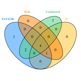
Figure 1: Venn diagram of the differential correlation pattern of the targeted gene pairs for the three weighting methods and unweighted analysis.

6 Conclusion

The integrative analysis of uncensored mixed-type multivariate outcomes in multiple retrospective cohorts to make unconfounded comparisons of multiple groups is a challenging problem. This paper formulates new frameworks for covariate-balanced pseudo-populations that extend, in a relatively straightforward manner, existing weighting methods to meta-analytical investigations. We propose generally applicable weighted estimators for a wide variety of population-level univariate or multivariate features relevant to multigroup comparisons, e.g., mean differences, linear contrasts and ratios of means, medians, and standard deviations, and pairwise correlation ceofficients. We evaluate the asymptotic properties of these estimators and develop small-sample bootstrap procedures for uncertainty estimation. The proposed approaches are applicable to meta-analytical extensions of various existing weighting methods, in addition to the novel, estimand-agnostic FLEXOR pseudo-population that maximizes the effective sample size by a cost-effective iterative procedure. Through simulation studies and data applications, we demonstrate the utility and effectiveness of these generally applicable inferential strategies.

The methodology can be potentially generalized in several directions, e.g., transportability (Westreich et al., 2017) and data-fusion (Bareinboim & Pearl, 2016) problems, which incorporate additional information in the form of random samples from the natural population. Furthermore, in recent years, weighting approaches are frequently challenged and rendered ineffectual by high-dimensional genetic or genomic measurements. Our future research will meet these challenges by extending the proposed approaches to these settings.

References

- (1)
- Austin (2010) Austin, P. C. (2010), ‘The performance of different propensity-score methods for estimating differences in proportions (risk differences or absolute risk reductions) in observational studies’, Statistics in Medicine 29(20), 2137–2148.
- Austin & Stuart (2015) Austin, P. C. & Stuart, E. A. (2015), ‘Moving towards best practice when using inverse probability of treatment weighting (IPTW) using the propensity score to estimate causal treatment effects in observational studies’, Statistics in Medicine 34(28), 3661–3679.
- Bareinboim & Pearl (2016) Bareinboim, E. & Pearl, J. (2016), ‘Causal inference and the data-fusion problem’, Proceedings of the National Academy of Sciences 113(27), 7345–7352.
- Bickel & Freedman (1981) Bickel, P. J. & Freedman, D. A. (1981), ‘Some asymptotic theory for the Bootstrap’, The Annals of Statistics 9(6), 1196 – 1217.
- Breiman (2001) Breiman, L. (2001), ‘Random Forests’, Machine Learning 45(1), 5–32.
- Christopoulos et al. (2015) Christopoulos, P. F., Msaouel, P. & Koutsilieris, M. (2015), ‘The role of the insulin-like growth factor-1 system in breast cancer’, Molecular Cancer 14(1), 1–14.
- Crump et al. (2006) Crump, R. K., Hotz, V. J., Imbens, G. W. & Mitnik, O. A. (2006), Moving the goalposts: addressing limited overlap in the estimation of average treatment effects by changing the estimand, Technical report, National Bureau of Economic Research.
- Efron & Tibshirani (1994) Efron, B. & Tibshirani, R. J. (1994), An introduction to the Bootstrap, CRC press.
- Feng et al. (2018) Feng, Y., Spezia, M., Huang, S., Yuan, C., Zeng, Z., Zhang, L., Ji, X., Liu, W., Huang, B., Luo, W. et al. (2018), ‘Breast cancer development and progression: Risk factors, cancer stem cells, signaling pathways, genomics, and molecular pathogenesis’, Genes & Diseases 5(2), 77–106.
- Hirano & Imbens (2001) Hirano, K. & Imbens, G. W. (2001), ‘Estimation of causal effects using propensity score weighting: an application to data on right heart catheterization’, Health Services and Outcomes Research Methodology 2(3), 259–278.
- Imbens (2000a) Imbens, G. W. (2000a), ‘The role of the propensity score in estimating dose-response functions’, Biometrika 87(3), 706–710.
- Imbens (2000b) Imbens, G. W. (2000b), ‘The role of the propensity score in estimating dose-response functions’, Biometrika 87(3), 706–710.
- Johnson et al. (2002) Johnson, R. A., Wichern, D. W. et al. (2002), Applied multivariate statistical analysis, Vol. 5, Prentice hall Upper Saddle River, NJ.
- Kumar et al. (2020) Kumar, B., Chand, V., Ram, A., Usmani, D. & Muhammad, N. (2020), ‘Oncogenic mutations in tumorigenesis and targeted therapy in breast cancer’, Current Molecular Biology Reports 6(3), 116–125.
- Li & Li (2019) Li, F. & Li, F. (2019), ‘Propensity score weighting for causal inference with multiple treatments’, The Annals of Applied Statistics 13(4), 2389–2415.
- Li et al. (2018) Li, F., Morgan, K. L. & Zaslavsky, A. M. (2018), ‘Balancing covariates via propensity score weighting’, Journal of the American Statistical Association 113(521), 390–400.
- Li & Greene (2013) Li, L. & Greene, T. (2013), ‘A weighting analogue to pair matching in propensity score analysis’, The International Journal of Biostatistics 9(2), 215–234.
- Lunceford & Davidian (2004) Lunceford, J. K. & Davidian, M. (2004), ‘Stratification and weighting via the propensity score in estimation of causal treatment effects: a comparative study’, Statistics in Medicine 23(19), 2937–2960.
- Malvia et al. (2019) Malvia, S., Bagadi, S. A. R., Pradhan, D., Chintamani, C., Bhatnagar, A., Arora, D., Sarin, R. & Saxena, S. (2019), ‘Study of gene expression profiles of breast cancers in indian women’, Scientific Reports 9(1), 1–15.
- McCaffrey et al. (2013) McCaffrey, D. F., Griffin, B. A., Almirall, D., Slaughter, M. E., Ramchand, R. & Burgette, L. F. (2013), ‘A tutorial on propensity score estimation for multiple treatments using generalized boosted models’, Statistics in Medicine 32(19), 3388–3414.
- NCI (2022) NCI (2022), ‘Genomic data commons data portal’. https://portal.gdc.cancer.gov/.
- Paul (2020) Paul, M. R. (2020), The Genomic Evolution of Breast Cancer Metastasis, PhD thesis, University of Pennsylvania.
- Robins et al. (2000) Robins, J. M., Hernan, M. A. & Brumback, B. (2000), ‘Marginal structural models and causal inference in epidemiology’, Epidemiology 11(5), 550–560.
- Robins & Rotnitzky (1995) Robins, J. M. & Rotnitzky, A. (1995), ‘Semiparametric efficiency in multivariate regression models with missing data’, Journal of the American Statistical Association 90(429), 122–129.
- Rosenbaum & Rubin (1983) Rosenbaum, P. R. & Rubin, D. B. (1983), ‘The central role of the propensity score in observational studies for causal effects’, Biometrika 70(1), 41–55.
- Rubin (2007) Rubin, D. B. (2007), ‘The design versus the analysis of observational studies for causal effects: parallels with the design of randomized trials’, Statistics in Medicine 26, 20–36.
- Rubin (2008) Rubin, D. B. (2008), ‘For objective causal inference, design trumps analysis’, The Annals of Applied Statistics pp. 808–840.
- Schmidt et al. (2016) Schmidt, K. T., Chau, C. H., Price, D. K. & Figg, W. D. (2016), ‘Precision oncology medicine: the clinical relevance of patient-specific biomarkers used to optimize cancer treatment’, The Journal of Clinical Pharmacology 56(12), 1484–1499.
- Singh (1981) Singh, K. (1981), ‘On the asymptotic accuracy of Efron’s bootstrap’, The Annals of Statistics 9(6), 1187–1195.
- Surveillance Research Program, NCI (2023) Surveillance Research Program, NCI (2023), ‘SEER*Explorer: An interactive website for SEER cancer statistics [Internet]’. Available from https://seer.cancer.gov/statistics-network/explorer/.
- Tran (2022) Tran, H.-T. (2022), ‘Invasive lobular carcinoma’. https://www.hopkinsmedicine.org/health/conditions-and-diseases/breast-cancer/invasive-lobular-carcinoma.
- Van der Vaart (2000) Van der Vaart, A. W. (2000), Asymptotic Statistics, Cambridge University Press.
- Wang & Rosner (2019) Wang, C. & Rosner, G. L. (2019), ‘A Bayesian nonparametric causal inference model for synthesizing randomized clinical trial and real-world evidence’, Statistics in Medicine 38(14), 2573–2588.
- Westreich et al. (2017) Westreich, D., Edwards, J. K., Lesko, C. R., Stuart, E. & Cole, S. R. (2017), ‘Transportability of trial results using inverse odds of sampling weights’, American journal of epidemiology 186(8), 1010–1014.
- Williams et al. (2022) Williams, R., Jobling, S., Sims, A. H., Mou, C., Wilkinson, L., Collu, G. M., Streuli, C. H., Gilmore, A. P., Headon, D. J. & Brennan, K. (2022), ‘Elevated edar signalling promotes mammary gland tumourigenesis with squamous metaplasia’, Oncogene 41(7), 1040–1049.
- Wright (2022) Wright, P. (2022), ‘Invasive ductal carcinoma’. https://www.hopkinsmedicine.org/health/conditions-and-diseases/breast-cancer/invasive-ductal-carcinoma-idc.
- Zielińska & Katanaev (2020) Zielińska, K. A. & Katanaev, V. L. (2020), ‘The signaling duo cxcl12 and cxcr4: Chemokine fuel for breast cancer tumorigenesis’, Cancers 12(10), 3071.
- Zonderman et al. (2014) Zonderman, A. B., Ejiogu, N., Norbeck, J. & Evans, M. K. (2014), ‘The influence of health disparities on targeting cancer prevention efforts’, American Journal of Preventive Medicine 46(3), S87–S97.